1 Introduction
Starting from the development of tomography and related techniques, the last fifty years have seen a constant rise in interest in the development of inverse problems as a research field, in mathematics as well as applied fields such as medical imaging, geophysics and the oil industry, or the steel industry, to mention only a few: see, for example, Bertero and Boccacci (Reference Bertero and Boccacci1998), Cakoni and Colton (Reference Cakoni and Colton2005), Chadan, Colton, Päivärinta and Rundell (Reference Chadan, Colton, Päivärinta and Rundell1997), Colton and Kress (Reference Colton and Kress2012), Colton et al. (Reference Colton, Engl, Louis, Mclaughlin and Rundell2012), Engl, Louis and Rundell (Reference Engl, Louis and Rundell2012), Groetsch (Reference Groetsch1993), Isakov (Reference Isakov2006, Reference Isakov2008), Natterer (Reference Natterer2001), Natterer and Wübbeling (Reference Natterer and Wübbeling2001), Tarantola and Valette (Reference Tarantola and Valette1982) and Tarantola (Reference Tarantola2005). Connected with the rise of interest in inverse problems is the development and analysis of regularization methods, which are a necessity in most inverse problems due to their ill-posedness: see, for example, Tikhonov, Goncharsky and Bloch (Reference Tikhonov, Goncharsky and Bloch1987) and Engl, Hanke and Neubauer (Reference Engl, Hanke and Neubauer1996). In particular there is usually no continuous dependence between the data and the solution of the inverse problem, hence in the presence of measurement errors one solves approximate problems with stable dependence instead. The controlled construction and analysis of such modified problems is called regularization, usually with a regularization parameter encoding the level of the approximation.
The canonical example of an ill-posed inverse problem at the abstract level is the linear operator equation
 $$\begin{eqnarray}Ku=f,\end{eqnarray}$$
with a linear operator
 $K$
between Banach spaces, whose generalized inverse
 $K^{\dagger }$
is unbounded. A regularization method is then some parametric approximation
 $R_{\unicode[STIX]{x1D6FC}}$
of
 $K^{\dagger }$
, which has better stability properties. In the case of linear regularization methods,
 $R_{\unicode[STIX]{x1D6FC}}$
is a family of bounded linear operators converging pointwise to
 $K^{\dagger }$
on the domain of the latter as
 $\unicode[STIX]{x1D6FC}\rightarrow 0$
. A key question in this respect is the convergence for noisy data, related to the choice of the regularization parameter
 $\unicode[STIX]{x1D6FC}$
in dependence on the noise level
 $\unicode[STIX]{x1D6FF}$
, the latter being a bound for the noise in the deterministic setting or some kind of variance in a stochastic setting.
At the end of the twentieth century, when rather complete understanding of such linear regularization methods was available (based on spectral decompositions of the operators), nonlinear regularization methods, i.e. nonlinear maps
 $R_{\unicode[STIX]{x1D6FC}}$
(possibly even multivalued), were becoming a field of intensive study. This was driven in particular by developments related to variational methods such as total variation techniques (Rudin, Osher and Fatemi Reference Rudin, Osher and Fatemi1992, Acar and Vogel Reference Acar and Vogel1994, Burger and Osher Reference Burger, Osher and Burger2013) or sparsity and compressed sensing (Donoho Reference Donoho2006, Donoho, Elad and Temlyakov Reference Donoho, Elad and Temlyakov2006, Candès and Donoho Reference Candès and Donoho2002), but also by statistical approaches such as advanced Bayesian prior models (Lassas, Saksman and Siltanen Reference Lassas, Saksman and Siltanen2009, Helin and Lassas Reference Helin and Lassas2011, Kolehmainen, Lassas, Niinimäki and Siltanen Reference Kolehmainen, Lassas, Niinimäki and Siltanen2012). Due to the rise of big data and learning techniques, in recent years there has been further interest in applying such paradigms to inverse problems. This is a somewhat delicate task, since in most inverse problems there are no ground truth data, but only results that have been reconstructed via a certain regularization method and specific noise. Hence there are many challenges for future research.
In this paper we will provide a survey of developments in the analysis and applications of modern (nonlinear) regularization methods during the last few decades. Moreover, we will try to provide a fairly structured overview of this field, including some fundamentals of nonlinear regularization methods. In particular we will give clear definitions as to what to expect from a regularization method and its convergence, reminiscent of the rather complete treatment of linear regularization methods in the seminal book by Engl, Hanke and Neubauer (Reference Engl, Hanke and Neubauer1996), now dating back more than twenty years.
Throughout the paper we assume that
 $K:{\mathcal{U}}\rightarrow {\mathcal{V}}$
is a bounded linear operator on Banach spaces
 ${\mathcal{U}}$
and
 ${\mathcal{V}}$
. In many parts there are obvious extensions to nonlinear operators and even metric spaces, but we mainly leave them out in order to increase readability; some links to such extensions are given at the end of the paper.
We will start in Section 2 with a historical exposition on regularization methods, and then proceed in Section 3 to nonlinear variational models, which are the class of methods driving most development in nonlinear regularizations. Section 4 will discuss some basic properties of and requirements on regularization methods, which are then discussed in detail for variational regularization in Section 5. Subsequently we turn to iterative regularization methods in Section 6. As a result of certain insights in these sections we are led to a discussion on bias and scales in regularization methods in Section 7, and Section 8 will provide some examples of applications. Section 9 will discuss advanced aspects such as nonlinear regularization methods for nonlinear inverse problems and links to machine learning. Finally we conclude and provide an outlook to relevant future topics in Section 10.
2 A little history of regularization methods
It seems difficult to date the origin of regularization methods, but it is now common to identify it with the pioneering work of Tikhonov (Reference Tikhonov1943, Reference Tikhonov1963, Reference Tikhonov1966) and the subsequent strong developments in the Russian community in the 1960s (e.g. Ivanov Reference Ivanov1962, Bakushinskii Reference Bakushinskii1967). The starting motivation obviously comes from the concept of ill-posedness, negating the definition of a well-posed problem. The latter, consisting of existence, uniqueness and stable dependence upon the input data, is usually attributed to the work of Hadamard in the context of partial differential equations (Hadamard Reference Hadamard1902, Reference Hadamard1923). However, the third condition was not clearly formulated in those problems, and only later found its true place of importance, for example in the work of John (Reference John1960). As a motivation for regularization theory and in particular for convergence theory, however, the lack of stability seems to be the most crucial issue.
It was already understood in early work that in order to have any chance of computing meaningful solutions, the problem needs to be approximated by well-posed ones, usually a family parametrized by the regularization parameter. The obvious first answer of a topologist such as Tikhonov was to restrict the domain to a compact set in some topology (or some kind of family thereof), leading to the concept of conditional well-posedness. A natural choice in a Hilbert space is to use norm balls centred at zero, which are compact in the weak topology. The radius of the ball (or its inverse) can naturally serve as a regularization parameter. This was also called the selection method, and the corresponding solutions were termed quasi-solutions. Given a minimization problem, e.g. least-squares
 $\Vert Ku-f\Vert ^{2}$
for (1.1) in Hilbert spaces, it is a shortcut to the variational formulation (see Section 3 for a detailed discussion of variational models) of what is now called Tikhonov or Tikhonov–Phillips regularization. Indeed, with an appropriate Lagrange parameter
 $\unicode[STIX]{x1D6FC}$
, this is equivalent to the variational problem
 $$\begin{eqnarray}\hat{u} =\underset{u\in {\mathcal{U}}}{\operatorname{argmin}}\,\displaystyle \frac{1}{2}\Vert Ku-f\Vert ^{2}+\displaystyle \frac{\unicode[STIX]{x1D6FC}}{2}\Vert u\Vert ^{2}.\end{eqnarray}$$
Some of the early work in the Soviet community was already formulated in a much more general variational way, replacing the least-squares term with some discrepancy measure and the regularization with an appropriate functional, in some sense a precursor of the modern theory. At this time the study was restricted to a rather abstract way of focusing on convergence proofs: strong motivations for other functionals in inverse problems and further methods for quantitative estimates were not available. The concepts and methods were further developed in the Soviet literature, including the question of the regularization parameter choice in dependence on the noise level. Instead of giving a detailed overview we refer to the influential book by Tikhonov and Arsenin (Reference Tikhonov and Arsenin1977), which also made the results more broadly accessible.
As an alternative approach much work also considered what Tikhonov called the regularization method (and what seems to be the first appearance of this term in the literature), namely the approximation of
 $K$
by regular operators and of its generalized inverse by bounded operators. There was parallel development in the West: Phillips (Reference Phillips1962) developed an approach similar to Tikhonov’s conditional well-posedness for integral equations of the first kind, and consequently the term Tikhonov–Phillips regularization is also used in the literature. In a discrete setting of statistical regression, a similar idea for dealing with ill-conditioned problems was developed under the term ridge regression (Hoerl Reference Hoerl1959, Hoerl and Kennard Reference Hoerl and Kennard1970). A related approach for solving ill-posed problems for partial differential equations was the quasi-reversibility method (Lattès and Lions Reference Lattès and Lions1967), although barely analysed in the setting of a regularization method.
A different route to the construction of regularization methods was taken by Backus and Gilbert (Reference Backus and Gilbert1968) from a very applied perspective. Using linear filters, the noisy data were smoothed to be in the range of the forward operator
 $K$
, followed by direct inversion (or a generalized inverse). It took quite a while for such methods to be understood in a unified way with other regularizations such as Tikhonov regularization (Engl et al.
Reference Engl, Hanke and Neubauer1996). The key step was to relate the smoothing action of the filters to the operator
 $K$
and its adjoint. This was made clear later in the linear functional strategy by Anderssen (Reference Anderssen, Cannon and Hornung1986) and also in the development of the approximate inverse method by Louis (Reference Louis1996), which turned out to be highly useful in tomography problems, where explicit reconstruction formulas and fast methods for the computation of the inverse are available.
In the 1970s and 1980s the study of linear regularization methods progressed further, dealing with many different regularization techniques such as iterative regularization by early stopping of stable iteration methods, truncated singular value decompositions, and regularization by discretization and projection (e.g. Nashed and Wahba Reference Nashed and Wahba1974b , Nashed and Wahba Reference Nashed and Wahba1974c , Wahba Reference Wahba1977, Eldén Reference Eldén1977, Bakushinskii Reference Bakushinskii1977, Bakushinskii Reference Bakushinskii1979, Bates and Wahba Reference Bates and Wahba1983, Engl Reference Engl1987b , Hansen Reference Hansen1987). Most work was based on using spectral methods for the construction and detailed analysis of regularization methods. This includes the basic analysis of linear regularization methods in Hilbert spaces, their convergence as the noise level and the regularization parameter tend to zero, as well as the first error estimates giving dependence on the noise level (e.g. Nashed and Wahba Reference Nashed and Wahba1974a , Groetsch and King Reference Groetsch and King1979, Natterer Reference Natterer1984, Neubauer Reference Neubauer1988a ). Moreover, various asymptotic parameter choice rules were suggested and investigated, either founded by theory such as the discrepancy principle or other a posteriori rules using the noise level (Morozov Reference Morozov1966, Bakushinskii Reference Bakushinskii1973, Raus Reference Raus1984, Engl and Neubauer Reference Engl, Neubauer, Hämmerlin and Hoffmann1985, Engl Reference Engl1987a , Engl and Neubauer Reference Engl, Neubauer, Engl and Groetsch1987, Gfrerer Reference Gfrerer1987, Engl and Gfrerer Reference Engl and Gfrerer1988, Raus Reference Raus1992), or heuristic ones such as quasi-optimality or the L-curve method (Tikhonov and Arsenin Reference Tikhonov and Arsenin1977, Bakushinskii Reference Bakushinskii1984, Thompson, Brown, Kay and Titterington Reference Thompson, Brown, Kay and Titterington1991, Hansen Reference Hansen1992). The development of linear regularization methods in the early 1990s was rather complete, culminating in the seminal book by Engl, Hanke and Neubauer (Reference Engl, Hanke and Neubauer1996), which provides a unified overview.
From the application point of view, a strong focus was placed on models with integral equations of the first kind, and image reconstruction in tomography drove applications (Natterer Reference Natterer2001, Natterer and Wübbeling Reference Natterer and Wübbeling2001 and references therein). In parallel, various applications of inverse problems in partial differential equations, such as inverse scattering or parameter identifications, became relevant and were tackled by regularization methods (e.g. Payne Reference Payne1975, Kravaris and Seinfeld Reference Kravaris and Seinfeld1985, Colton and Monk Reference Colton and Monk1988, Banks and Kunisch Reference Banks and Kunisch1989, Colton et al. Reference Colton, Ewing and Rundell1990). This drove the interest in regularization theory from linear towards nonlinear problems.
The end of the 1980s marks the beginning of the systematic analysis of regularization methods for nonlinear inverse problems (replacing
 $K$
with a nonlinear operator). In particular, the papers by Seidman and Vogel (Reference Seidman and Vogel1989) gave a well-posedness and convergence analysis of Tikhonov regularization for such problems, and Engl, Kunisch and Neubauer (Reference Engl, Kunisch and Neubauer1989) provided the first error estimates and convergence rates. Many techniques had to be developed to avoid spectral theory arguments that are not available for nonlinear operators; it is not surprising that many of those ideas were also influential for nonlinear regularization (of linear inverse problems). In the 1990s there was a surge in studies for nonlinear inverse problems. In particular, a theory of iterative regularization methods was constructed, which is particularly attractive since the nonlinear problems had to be solved with iterative methods in any case. Prominent examples are Landweber and steepest-descent methods (e.g. Hanke, Neubauer and Scherzer Reference Hanke, Neubauer and Scherzer1995), regularized Newton methods (e.g. Kaltenbacher Reference Kaltenbacher1997) and iterated Tikhonov methods (e.g. Scherzer Reference Scherzer1993). We refer to Kaltenbacher, Schöpfer and Schuster (Reference Kaltenbacher, Schöpfer and Schuster2009) for a comprehensive overview.
In parallel, another paradigm evolved, particularly in the image processing community, from the seminal papers of Rudin et al. (Reference Rudin, Osher and Fatemi1992) and Mumford and Shah (Reference Mumford and Shah1989), who proposed nonlinear variational models to solve denoising (and in the second case also segmentation) problems. From a regularization point of view this means that a nonlinear regularization method is used to solve a linear inverse problem, a rather unusual idea at this time. From a technical point of view it poses the additional challenge of analysing schemes in anisotropic Banach spaces, such as the space of functions of bounded variation, while theory was previously formulated mainly in Hilbert spaces. In the case of variational regularization methods, basic well-posedness and convergence analysis can be carried out using techniques from variational calculus (Acar and Vogel Reference Acar and Vogel1994, Eggermont Reference Eggermont1993), while quantitative estimates need completely novel approaches. Early progress in this direction was made for maximum entropy regularization (Eggermont Reference Eggermont1993, Engl and Landl Reference Engl and Landl1993); in this case the regularization technique could be related directly to regularization of nonlinear inverse problems in Hilbert spaces via a change of variables (Engl and Landl Reference Engl and Landl1993). However, in a more general set-up the convergence rate theory remained quite open until the dawn of the twenty-first century, when strong progress was made by employing techniques from convex analysis to variational regularization methods. We mention at this point that some of these more geometric ideas were also hidden in earlier work on regularization in Hilbert spaces with convex constraints (Neubauer Reference Neubauer1988b , Eicke Reference Eicke1992). The improved understanding of variational regularization methods in Banach spaces subsequently led to a variety of other techniques and variants, such as derived iterative regularization, which we will discuss in further detail in the course of this paper.
Another driving force for investigating regularization methods in Banach spaces was sparsity, including wavelet shrinkage and the variational counterpart of regularization
 $\ell ^{1}$
-type norms, for example in Besov spaces (Donoho Reference Donoho1992, Donoho and Johnstone Reference Donoho and Johnstone1995). This led in parallel to the field of compressed sensing, where the focus was on designing the appropriate measurement set-ups for optimal compression rather than improving reconstructions on a given inverse problem (Donoho Reference Donoho2006, Candès, Romberg and Tao Reference Candès, Romberg and Tao2006, Candès and Donoho Reference Candès and Donoho2002, Candès and Tao Reference Candès and Tao2004a
, Candès and Tao Reference Candès and Tao2004b
, Candès and Romberg Reference Candès and Romberg2007, Donoho et al.
Reference Donoho, Elad and Temlyakov2006). Despite the fact that the usual setting in compressed sensing is a finite-dimensional one, many arguments based on convex analysis are closely related.
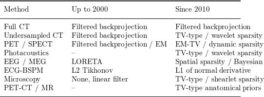
In recent years these techniques also evolved into many practical applications, in particular in the image reconstruction community. The whole list of applications where the methods made an impact in different ways might warrant its own survey paper. In order to illustrate the change in the first decade of the twentieth century we provide Table 2.1, which shows the typical state of the art for inverse problems in medical imaging up to or around the year 2000 and that typically used ten years later.
State of the art for inverse problems in medical imaging.

Note that (with the exception of the statistically motivated EM algorithm) all state-of-the-art methods up to 2000 were linear regularization methods. This has now completely changed, with the exception of fully sampled CT, where there is neither a null space nor significant noise, and hence regularization plays a minor role. The details of most other methods, mainly based on variational models, will become clear in the next section.
3 Variational modelling
The variational approach to regularization methods has become very popular in the last few decades, since it provides an intuitive approach to modelling and a framework for its basic analysis, and also allows a variety of computational methods to be applied, particularly in the case of convex regularization functionals. The key idea in constructing a variational regularization method for (1.1) consists of finding two functionals: a data fidelity term
 $F$
measuring the distance between
 $Ku$
and
 $f$
(or its noisy version
 $f^{\unicode[STIX]{x1D6FF}}$
) and a regularization functional
 $J$
favouring appropriate minimizers or penalizing potential solutions with undesired structures. Instead of simply fitting
 $u$
to data, i.e. minimizing
 $F(Ku,f)$
, a weighted version is minimized to obtain
 $$\begin{eqnarray}\hat{u} \in \underset{u}{\operatorname{argmin}}\,(F(Ku,f^{\unicode[STIX]{x1D6FF}})+\unicode[STIX]{x1D6FC}J(u)),\end{eqnarray}$$
where
 $\unicode[STIX]{x1D6FC}>0$
is the regularization parameter controlling the influence of the two terms on the minimizer. Since the problem should approach the minimization of only the data fidelity term in the noiseless case, it is natural to think of
 $\unicode[STIX]{x1D6FC}$
as a small parameter.
The choice of the data fidelity term is often straightforward, for example as some kind of least-squares term (squared norm distance in a Hilbert space), or motivated from statistical arguments by some likelihood functional for the noise. In the latter case the variational model can be interpreted as a regularized likelihood model, where the data term usually corresponds to the negative log likelihood of the noise model. A prominent example is the case of additive Gaussian noise, which leads to a least-squares data term
 ${\textstyle \frac{1}{2}}\Vert Ku-f\Vert ^{2}$
, where the specific Hilbert space norm to be used is determined by the covariance operator of the noise. Appropriate choices for the latter can have a significant impact: for example, choosing likelihoods for Poisson noise appearing in photon count data leads to strong improvement over least-squares terms, particularly in large noise regimes (e.g. Sawatzky et al. Reference Sawatzky, Brune, Kösters, Wübbeling, Burger, Burger and Osher2013, Brune, Sawatzky and Burger Reference Brune, Sawatzky and Burger2009c
). Throughout this paper we will assume that
 $F$
is Fréchet-differentiable on
 ${\mathcal{V}}$
unless otherwise stated.
The choice of a regularization functional seems less natural at first glance. Based on the original ideas by Tikhonov, the key ingredient for a successful regularization is its topological properties, so the regularization functional is frequently chosen as some power of a norm (or seminorm) in a Banach space. Classical examples are Tikhonov–Phillips in Hilbert spaces such as
 $L^{2}(\unicode[STIX]{x1D6FA})$
,
 $H^{1}(\unicode[STIX]{x1D6FA})$
, or in some sequence space
 $\ell ^{2}(\mathbb{N})$
. As a generalization in function spaces, regularization functionals depending on the gradient (or higher-order derivatives) of
 $u$
became popular. These correspond to the rather direct intuition that smooth solutions are preferable due to prior knowledge. Non-smooth and oscillatory functions will lead to large or even infinite values of the derivatives, and thus very high values of the regularization functionals. Hence, they are not suitable candidates as a minimizer of (3.1).
In many cases in inverse problems such as image reconstruction, one is instead interested in non-smooth solutions, and in particular their discontinuity sets. One example is that of piecewise constant functions with reasonable edge sets, which are not contained in any Sobolev space
 $W^{k,p}(\unicode[STIX]{x1D6FA})$
for
 $k,p\geq 1$
, since their gradient is already a concentrated measure (Ambrosio, Fusco and Pallara Reference Ambrosio, Fusco and Pallara2000, Evans and Gariepy Reference Evans and Gariepy1992). This motivates use of the space of functions of bounded variations
 $BV(\unicode[STIX]{x1D6FA})$
, which consists of all functions in
 $L^{1}(\unicode[STIX]{x1D6FA})$
whose distributional gradients are vectorial Radon measures. The regularization with the total variation, that is,
 $$\begin{eqnarray}TV(u)=|u|_{BV}=\int _{\unicode[STIX]{x1D6FA}}\,\text{d}|Du|,\end{eqnarray}$$
where
 $Du$
is the gradient measure of
 $u$
, proposed for denoising by Rudin et al. (Reference Rudin, Osher and Fatemi1992), and the subsequent popularity of investigating such methods can be seen as the advent of modern regularization methods.
The details of reconstructions to be achieved, however, strongly depend on the specific norm used. It is common folklore that the regularization functional is chosen such that desired solutions matching prior knowledge have a small value of
 $J$
and are thus preferred as the appropriate solutions. This is true only to some extent, but the overall effect of a regularization functional is determined by the effect it has on possible minimizers rather than purely a comparison of functional values. Consider as a simple example one-dimensional total variation regularization. It will of course prefer solutions with small total variation over oscillatory functions with high variation. On the other hand, it still selects among functions with the same total variation. Structural results on the solution of total variation regularization problems show that canonical solutions for noisy data are piecewise constant, even if the exact solution is not (Ring Reference Ring2000, Chambolle et al.
Reference Chambolle, Caselles, Cremers, Novaga, Pock and Fornasier2010, Jalalzai Reference Jalalzai2016). This means that total variation actively selects piecewise constant solutions over smooth solutions that have the same total variation, that is, they are a priori indistinguishable by the regularization functional. The reason for this behaviour can be seen by inspecting the optimality condition, given by (assuming
 $F$
to be Fréchet-differentiable)
 $$\begin{eqnarray}K^{\ast }\unicode[STIX]{x2202}_{x}F(Ku,f)+\unicode[STIX]{x1D6FC}p=0,\quad p\in \unicode[STIX]{x2202}J(u).\end{eqnarray}$$
Here
 $\unicode[STIX]{x2202}_{x}$
denotes the (partial) Fréchet derivative in the first argument, and
 $\unicode[STIX]{x2202}J(u)$
is the subdifferential of
 $J$
at position
 $u$
: see Rockafellar (Reference Rockafellar1972, Section 23) or Ekeland and Temam (Reference Ekeland and Temam1999). Solving for the subgradient
 $p$
, we always obtain a relation of the form
 $p=K^{\ast }\tilde{w}$
for some
 $\tilde{w}\in {\mathcal{V}}$
, that is, the variational method will select smooth subgradients due to the smoothing properties of the operator
 $K$
and its adjoint. We will detail the relation between the properties of the subgradients of the solution for total variation and other examples of regularization in the next sections.
In a stochastic set-up, the variational approach is often formulated from Bayesian estimation (Kaipio and Somersalo Reference Kaipio and Somersalo2006, Stuart Reference Stuart2010), in particular maximum a posteriori probability (MAP) estimators. For the sake of simpler presentation, assume that we are in a finite-dimensional setting for the inverse problem
 $Ku=f$
and can write down probability densities for the prior
 $\unicode[STIX]{x1D70B}_{0}(u)$
and the likelihood
 $\unicode[STIX]{x1D70B}(f|u)$
of measuring the data
 $f$
given the true solution
 $u$
. Then Bayes’ theorem provides the posterior probability density via
 $$\begin{eqnarray}\unicode[STIX]{x1D70B}(u|f)=\displaystyle \frac{1}{\unicode[STIX]{x1D70B}_{\ast }(f)}\unicode[STIX]{x1D70B}(f|u)\unicode[STIX]{x1D70B}_{0}(u),\end{eqnarray}$$
where
 $$\begin{eqnarray}\unicode[STIX]{x1D70B}_{\ast }(f)=\int \unicode[STIX]{x1D70B}(f|u)\unicode[STIX]{x1D70B}_{0}(u)\,\text{d}u\end{eqnarray}$$
is the effective prior probability on the data. A MAP estimate
 $\hat{u}$
is defined as a maximizer of the posterior probability density, or a minimizer of its negative logarithm. Since the part
 $\unicode[STIX]{x1D70B}_{\ast }(f)$
independent of
 $u$
is irrelevant for the minimizer, we thus have
 $$\begin{eqnarray}\hat{u} \in \underset{u}{\operatorname{argmin}}\,(-\log \unicode[STIX]{x1D70B}(f|u)-\log \unicode[STIX]{x1D70B}_{0}(u)).\end{eqnarray}$$
This formulation is closely related to the variational modelling point of view when interpreting
 $-\log \unicode[STIX]{x1D70B}(f|u)$
as a data fidelity term and
 $-\log \unicode[STIX]{x1D70B}_{0}(u)$
as the regularization term. Indeed, for many standard stochastic (noise) models one obtains
 $$\begin{eqnarray}\unicode[STIX]{x1D70B}(f|u)\sim \exp (-F(Ku,f)).\end{eqnarray}$$
Examples are additive Gaussian noise leading to a least-squares fidelity and Poisson noise leading to the Kullback–Leibler divergence. Assuming further that the prior is related to some regularization functional
 $J$
,
 $$\begin{eqnarray}\unicode[STIX]{x1D70B}_{0}(u)\sim \unicode[STIX]{x1D6F7}(-J(u)),\end{eqnarray}$$
for some monotone function
 $\unicode[STIX]{x1D6F7}$
, we see that the MAP estimation problem becomes
 $$\begin{eqnarray}\hat{u} \in \underset{u}{\operatorname{argmin}}\,F(Ku,f)-\log (\unicode[STIX]{x1D6F7}(-J(u))).\end{eqnarray}$$
This problem can be reformulated in a more conventional form, even if the prior
 $\unicode[STIX]{x1D6F7}$
is not exactly specified. By a standard argument we see that there exists
 $\unicode[STIX]{x1D6FE}>0$
such that
 $$\begin{eqnarray}\hat{u} \in \underset{u,J(u)\leq \unicode[STIX]{x1D6FE}}{\operatorname{argmin}}\,F(Ku,f),\end{eqnarray}$$
and with the existence of a Lagrange parameter
 $\unicode[STIX]{x1D6FC}>0$
for the constraint
 $J(u)\leq \unicode[STIX]{x1D6FE}$
(which is easily verified for a scalar constraint) we obtain
 $$\begin{eqnarray}\hat{u} \in \underset{u}{\operatorname{argmin}}\,F(Ku,f)+\unicode[STIX]{x1D6FC}J(u).\end{eqnarray}$$
We mention that similar reasoning in infinite dimensions is not as straightforward: even the definition of the MAP estimate is a non-obvious task (Dashti, Law, Stuart and Voss Reference Dashti, Law, Stuart and Voss2013, Helin and Burger Reference Helin and Burger2015). Recent results, however, provide good characterization in many relevant cases (Helin and Burger Reference Helin and Burger2015, Lie and Sullivan Reference Lie and Sullivan2017, Agapiou, Burger, Dashti and Helin Reference Agapiou, Burger, Dashti and Helin2018). A relation between Bayesian estimators and the variational approach also exists beyond the MAP estimate by the Bayes cost method. Given a cost
 $\unicode[STIX]{x1D713}$
measuring a distance on the input space, the Bayes cost approach looks for a minimizer of the posterior expectation of
 $\unicode[STIX]{x1D713}$
, that is,
 $$\begin{eqnarray}\hat{u} \in \underset{u}{\operatorname{argmin}}\,\int \unicode[STIX]{x1D713}(u,v)~\unicode[STIX]{x1D70B}(v|f)\,\text{d}v,\end{eqnarray}$$
a functional that depends in a more implicit way on the data and the forward model.
3.1 Total variation and related regularizations
As mentioned above, total variation regularization has been one of the driving examples for development of regularization methods in Banach spaces starting from Rudin et al. (Reference Rudin, Osher and Fatemi1992) and Acar and Vogel (Reference Acar and Vogel1994). Since then it has been a constant source of motivation for further development of mathematical analysis (e.g. Chambolle and Lions Reference Chambolle and Lions1997, Strong et al. Reference Strong and Chan1996, Scherzer Reference Scherzer1998, Chavent and Kunisch Reference Chavent and Kunisch1997, Ring Reference Ring2000, Strong and Chan Reference Strong and Chan2003, Burger and Osher Reference Burger and Osher2004, Caselles, Chambolle and Novaga Reference Caselles, Chambolle and Novaga2007, Allard Reference Allard2007), computational optimization techniques for non-smooth problems (e.g. Chan, Golub and Mulet Reference Chan, Golub and Mulet1999, Vogel Reference Vogel2002, Chambolle Reference Chambolle2004, Kunisch and Hintermüller Reference Kunisch and Hintermüller2004, Chambolle and Pock Reference Chambolle and Pock2011), and development of advanced models (e.g. Scherzer Reference Scherzer1998, Osher et al. Reference Osher, Burger, Goldfarb, Xu and Yin2005, Burger, Osher, Xu and Gilboa Reference Burger, Osher, Xu, Gilboa and Paragios2005, Burger et al. Reference Burger, Gilboa, Osher and Xu2006, Bredies and Holler Reference Bredies and Holler2015a , Hu and Jacob Reference Hu and Jacob2012, Lenzen, Becker and Lellmann Reference Lenzen, Becker, Lellmann and Aujol2013, Benning, Brune, Burger and Müller Reference Benning, Brune, Burger and Müller2013).
The key step for modern analysis and computational methods is the (pre-) dual formulation of total variation,
 $$\begin{eqnarray}TV(u)=|u|_{BV}:=\sup _{g\in C_{0}^{\infty }(\unicode[STIX]{x1D6FA})^{d},g\in {\mathcal{C}}}\int _{\unicode[STIX]{x1D6FA}}u\unicode[STIX]{x1D6FB}\cdot g\,\text{d}x,\end{eqnarray}$$
with the convex set
 $$\begin{eqnarray}{\mathcal{C}}=\{g\in L^{\infty }(\unicode[STIX]{x1D6FA})\mid |g(x)|\leq 1\text{ a.e. in }\unicode[STIX]{x1D6FA}\}.\end{eqnarray}$$
This characterization allows us to understand the structure of subgradients as elements of
 ${\mathcal{C}}$
absolutely continuous with respect to the gradient measure
 $D$
such that
 $$\begin{eqnarray}\int _{\unicode[STIX]{x1D6FA}}g\cdot \,\text{d}Du=|u|_{BV}.\end{eqnarray}$$
The optimality condition (3.3) provides
 $$\begin{eqnarray}K^{\ast }\unicode[STIX]{x2202}_{x}F(Ku,f)+\unicode[STIX]{x1D6FC}\unicode[STIX]{x1D6FB}\cdot g=0,\end{eqnarray}$$
where
 $g$
is a vector field such that
 $g|Du|$
is a polar decomposition of the vector measure (Ambrosio et al.
Reference Ambrosio, Fusco and Pallara2000).
In one spatial dimension the structure of solutions can be understood directly from the optimality condition. If there is an open set where
 $u$
is not constant, either with positive or negative derivative, then
 $g$
equals
 $+1$
or
 $-1$
, hence its derivative vanishes. Thus, in such regions the generalized residual
 $K^{\ast }\unicode[STIX]{x2202}_{x}F(Ku,f)$
vanishes. In the case of noisy data this is usually not happening for larger sets, thus
 $u$
is typically piecewise constant. In higher spatial dimensions this is not completely true, but still the case
 $|g(x)|<1$
is the canonical one, so in many cases solutions are piecewise constant. On the other hand, piecewise constant structures are not optimal in all instances. In particular, total variation methods are well known to exhibit staircasing phenomena, that is, smoothly varying parts in the solution are often approximated by piecewise constant structures with many jumps resembling a stair structure. For this reason many modifications and variants of total variation regularization have been investigated in recent decades. An immediate option is that of higher-order total variation approaches, which formally replace the one-norm of the gradient with the one-norm of a higher-order derivative such as the Laplacian, the Hessian or the symmetric part of the Hessian (e.g. Scherzer Reference Scherzer1998, Chan, Esedoglu and Park Reference Chan, Esedoglu and Park2010, Hinterberger and Scherzer Reference Hinterberger and Scherzer2006, Papafitsoros and Schönlieb Reference Papafitsoros and Schönlieb2014). The disadvantage of such an approach is that solutions of the regularization model will be too regular and discontinuity sets (edges) are lost. In view of (3.12) such approaches can be characterized by
 ${\mathcal{C}}$
not being a bounded set in
 $L^{\infty }(\unicode[STIX]{x1D6FA})$
, but rather being derivatives of bounded measurable functions.
An alternative model trying to take advantage of total variation and higher-order total variation is a decomposition into two or more parts, that is,
 $u=u_{1}+u_{2}$
with
 $u_{1}$
and
 $u_{2}$
being regularized differently. This was proposed for the first time by Chambolle and Lions (Reference Chambolle and Lions1997) as an infimal convolution of first- and second-order total variations; the effective regularization functional is given by
 $$\begin{eqnarray}J(u)=\inf _{u_{1}+u_{2}=u}(|u_{1}|_{BV}+|\unicode[STIX]{x1D6FB}u_{2}|_{BV}).\end{eqnarray}$$
The TGV-type models, proposed by Bredies, Kunisch and Pock (Reference Bredies, Kunisch and Pock2010), became a popular alternative. Instead of decomposing
 $u$
, these instead decompose the gradient measure
 $Du$
into
 $Du_{1}$
and some vector field
 $u_{2}$
. One version of the regularization functional is then given by
 $$\begin{eqnarray}J(u)=\inf _{Du_{1}+u_{2}=Du}(|u_{1}|_{BV}+|u_{2}|_{BV}).\end{eqnarray}$$
The fact that the higher-order part is an arbitrary vector field provides additional freedom that can be beneficial compared to the infimal convolution model (Bredies and Holler Reference Bredies and Holler2015a
, Benning, Brune, Burger and Müller Reference Benning, Brune, Burger and Müller2013, Grah Reference Grah2017). We also mention that the original TGV model in Bredies et al. (Reference Bredies, Kunisch and Pock2010) does not use a bounded variation model for
 $u_{2}$
, but only bounded deformations, that is, the symmetric part of the gradient. Moreover, the approach can be formulated for arbitrary order of regularization. In the dual formulation (3.12) approaches such as infimal convolution or TGV still lead to
 ${\mathcal{C}}$
being a subset of the unit ball in
 $L^{\infty }(\unicode[STIX]{x1D6FA})$
, which implies
 $$\begin{eqnarray}J(u)\leq |u|_{BV}\quad \text{for all}~u\in BV(\unicode[STIX]{x1D6FA}).\end{eqnarray}$$
On the other hand, for many of them a lower bound inequality can be shown at least when excluding a low- (finite-) dimensional null space (Benning et al.
Reference Benning, Brune, Burger and Müller2013), that is, there exists a positive constant
 $c$
and some linear functionals
 $\ell _{i}$
such that
 $$\begin{eqnarray}J(u)\geq c|u|_{BV}\quad \text{for all}~u\in BV(\unicode[STIX]{x1D6FA}),\quad \text{such that }\ell _{i}(u)=0,i=1,\ldots M.\end{eqnarray}$$
Hence,
 $J$
is an equivalent norm on the subspace of
 $BV$
excluding the null space. For the combination of first- and second-order derivatives the null space naturally consists of piecewise affine functions (thus
 $M=d+1$
). For further discussion and advanced aspects we refer to Bredies et al. (Reference Bredies, Kunisch and Pock2010), Benning et al. (Reference Benning, Brune, Burger and Müller2013), Ranftl, Pock and Bischof (Reference Ranftl, Pock, Bischof and Kuijper2013), Bredies and Holler (Reference Bredies and Holler2014, Reference Bredies and Holler2015a
, Reference Bredies and Holler2015b
), Burger, Papafitsoros, Papoutsellis and Schönlieb (Reference Burger, Papafitsoros, Papoutsellis, Schönlieb and Bociu2015b
, Reference Burger, Papafitsoros, Papoutsellis and Schönlieb2016c
), Bergounioux (Reference Bergounioux2016), Setzer, Steidl and Teuber (Reference Setzer, Steidl and Teuber2011), Holler and Kunisch (Reference Holler and Kunisch2014), Gao and Bredies (Reference Gao and Bredies2017) and Bergounioux and Papoutsellis (Reference Bergounioux and Papoutsellis2018).
In certain cases it is also interesting to use total variation regularization on some transform of the image. Motivated by research in image analysis taking into account orientations via local Radon transforms (Krause, Alles, Burgeth and Weickert Reference Krause, Alles, Burgeth and Weickert2016), Burger, Müller, Papoutsellis and Schönlieb (Reference Burger, Müller, Papoutsellis and Schönlieb2014) investigated total variation regularization on the Radon transform, combined with total variation on the image itself, to promote piecewise constant images with very thin structures resembling lines. Grah (Reference Grah2017) investigated total variation on the spherical Radon transform (equivalent to circular Hough transform in computer vision) in order to reconstruct small circular structures.
Another variant is total variation regularization for vector fields, for example arising for colour images (Bresson and Chan Reference Bresson and Chan2008, Blomgren and Chan Reference Blomgren and Chan1998), flow fields (Hinterberger, Scherzer, Schnörr and Weickert Reference Hinterberger, Scherzer, Schnörr and Weickert2002, Zach, Pock and Bischof Reference Zach, Pock, Bischof and Hamprecht2007) or joint reconstruction problems (Knoll et al.
Reference Knoll, Holler, Koesters, Otazo, Bredies and Sodickson2017). While many aspects remain the same as in the scalar case, it is particularly interesting to consider which matrix norm should be used for
 $Du$
, and which dual norm for
 $g$
(observing that this becomes a matrix in (3.12)).
3.2 Sparsity regularization
Total variation regularization, in particular its discrete version, can be interpreted as a functional favouring sparsity, in this case of the gradient. The paradigm of sparsity has developed in parallel to the total variation regularization (Donoho Reference Donoho1992). A key insight driving sparsity priors was the (approximate) sparsity of signals and natural images in wavelet bases (Mallat and Zhang Reference Mallat and Zhang1993, Huang and Mumford Reference Huang and Mumford1999, Mallat Reference Mallat2008, Starck, Murtagh and Fadili Reference Starck, Murtagh and Fadili2010). Further improvements were made by replacing the orthonormal bases with frames (Christensen Reference Christensen2003) such as curvelets (Candès and Donoho Reference Candès and Donoho2000a , Reference Candès and Donoho2000b ) or shearlets (Labate, Lim, Kutyniok and Weiss Reference Labate, Lim, Kutyniok and Weiss2005, Guo and Labate Reference Guo and Labate2007, Kutyniok and Labate Reference Kutyniok and Labate2012).
Sparsity is naturally measured by the
 $\ell ^{0}$
-norm,Footnote
1
the number of non-zero entries. Since the minimization of the
 $\ell ^{0}$
-norm is highly non-convex and even NP-complete, it is usually relaxed to the convex
 $\ell ^{1}$
-norm. In the analysis formulation a frame system
 $\unicode[STIX]{x1D719}_{i}$
is used to test sparsity of
 $\langle u,\unicode[STIX]{x1D719}_{i}\rangle$
, and the corresponding regularization functional is given by
 $$\begin{eqnarray}J(u)=\mathop{\sum }_{i}|\langle u,\unicode[STIX]{x1D719}_{i}\rangle |.\end{eqnarray}$$
If
 $(\unicode[STIX]{x1D719}_{i})$
is an orthonormal system, this is equivalent to the synthesis formulation, which is based on writing
 $$\begin{eqnarray}J(u)=\mathop{\sum }_{i}|c_{i}|\quad \text{where }u=\mathop{\sum }_{i}c_{i}\unicode[STIX]{x1D719}_{i}.\end{eqnarray}$$
Note that in general the two formulations may differ for frames (Elad, Milanfar and Rubinstein Reference Elad, Milanfar and Rubinstein2007).
In the synthesis formulation we can effectively define the variational problem on the coefficient vector
 $c$
, that is,
 $$\begin{eqnarray}\tilde{K}:\ell ^{2}(\mathbb{N})\rightarrow {\mathcal{V}},\quad c\mapsto \mathop{\sum }_{i}c_{i}K\unicode[STIX]{x1D719}_{i},\end{eqnarray}$$
and compute
 $$\begin{eqnarray}\hat{u} =\mathop{\sum }_{i}{\hat{c}}_{i}\unicode[STIX]{x1D719}_{i},\quad c_{i}\in \underset{c}{\operatorname{argmin}}\,F(\tilde{K}c,f)+\unicode[STIX]{x1D6FC}|c|_{1}.\end{eqnarray}$$
The corresponding optimality condition is given by
 $$\begin{eqnarray}(\tilde{K}^{\ast }\unicode[STIX]{x2202}_{x}F(\tilde{K}c,f))_{i}+\unicode[STIX]{x1D6FC}s_{i}=0,\end{eqnarray}$$
where
 $s_{i}$
is a multivalued sign of
 $c_{i}$
, that is, an element of
 $[-1,1]$
for
 $c_{i}=0$
. If
 $\tilde{K}$
is a bounded linear operator on
 $\ell ^{2}(\mathbb{N})$
, then its adjoint maps into the same space, and hence
 $(s_{i})\in \ell ^{2}(\mathbb{N})$
. This implies in particular that
 $|s_{i}|<1$
, hence
 $c_{i}=0$
, for
 $i$
sufficiently large. Thus, we always obtain some sparsity with this model.
In the analysis formulation the optimality condition is instead given by
 $$\begin{eqnarray}K^{\ast }\unicode[STIX]{x2202}_{x}F(Ku,f)+\unicode[STIX]{x1D6FC}s_{i}\unicode[STIX]{x1D719}_{i}=0,\end{eqnarray}$$
where
 $s_{i}$
is a multivalued sign for
 $\langle u,\unicode[STIX]{x1D719}_{i}\rangle$
. Here the understanding of the sparsity property is more complicated: the
 $s_{i}$
are actually related to the residual via the linear system
 $$\begin{eqnarray}\mathop{\sum }_{j}\langle \unicode[STIX]{x1D719}_{i},\unicode[STIX]{x1D719}_{j}\rangle s_{j}=-\displaystyle \frac{1}{\unicode[STIX]{x1D6FC}}\langle K\unicode[STIX]{x1D719}_{i},\unicode[STIX]{x2202}F(Ku,f)\rangle .\end{eqnarray}$$
We refer to Vaiter et al. (Reference Vaiter, Deledalle, Peyré, Dossal and Fadili2013a , Reference Vaiter, Peyré, Dossal and Fadili2013b ) for a detailed analysis in this case. Sparsity models for inverse problems have been studied with different frames and applications extensively in the past decade (e.g. Cotter, Rao, Engan and Kreutz-Delgado Reference Cotter, Rao, Engan and Kreutz-Delgado2005, Chaux, Combettes, Pesquet and Wajs Reference Chaux, Combettes, Pesquet and Wajs2007, Colonna, Easley, Guo and Labate Reference Colonna, Easley, Guo and Labate2010, Recht, Fazel and Parrilo Reference Recht, Fazel and Parrilo2010).
There are several relevant extensions of sparsity priors to multidimensional systems, in particular via a synthesis-type formulation:
 $$\begin{eqnarray}u=\mathop{\sum }_{i,j}c_{ij}\unicode[STIX]{x1D719}_{i}\otimes \unicode[STIX]{x1D713}_{j}.\end{eqnarray}$$
The different dimensions are often space (characterized by basis functions
 $\unicode[STIX]{x1D719}_{i}$
) and time or frequency (characterized by basis functions
 $\unicode[STIX]{x1D713}_{j}$
). Instead of overall sparsity, more detailed prior knowledge can be introduced. The most popular example is joint or collaborative sparsity, which means that only a few of the basis functions, for example in the second dimension, can be used to explain the solution. This means that
 $c_{\cdot j}$
vanishes for most
 $j$
, as does the norm of
 $c_{\cdot j}$
. A common regularization for this case is the joint or collaborative sparsity prior
 $$\begin{eqnarray}J(u)=\mathop{\sum }_{j}\Vert c_{\cdot j}\Vert _{\ell ^{r}},\end{eqnarray}$$
usually with
 $r=2$
or
 $r=\infty$
(Duarte et al.
Reference Duarte, Sarvotham, Wakin, Baron and Baraniuk2005, Teschke and Ramlau Reference Teschke and Ramlau2007, Fornasier and Rauhut Reference Fornasier and Rauhut2008, Gholami and Siahkoohi Reference Gholami and Siahkoohi2010, Lee, Kim, Bresler and Ye Reference Lee, Kim, Bresler and Ye2011). An alternative type of prior knowledge is local sparsity, which means that for each
 $i$
only a few basis functions
 $\unicode[STIX]{x1D713}_{j}$
are used. The term local is due to an imaging interpretation of the
 $\unicode[STIX]{x1D719}_{i}$
as basis functions local in space (e.g. for each pixel). This is a common issue in dynamic or spectral imaging, where one can assume that only a few materials and their characteristic evolutions or spectral curves can be found in each pixel. A regularization functional proposed for this issue (Heins, Moeller and Burger Reference Heins, Moeller and Burger2015) is
 $$\begin{eqnarray}J(u)=\max _{i}\Vert c_{i\cdot }\Vert _{\ell ^{1}}+\unicode[STIX]{x1D6FD}\mathop{\sum }_{i}\Vert c_{i\cdot }\Vert _{\ell ^{1}}.\end{eqnarray}$$
An infinite-dimensional extension of the above sparsity models is sparsity in a space of Radon measures, that is, the regularization functional is given as the total variation norm of the measure
 $u$
:
 $$\begin{eqnarray}J(u)=\int _{\unicode[STIX]{x1D6FA}}\,\text{d}|u|=\sup _{g\in C_{0}(\unicode[STIX]{x1D6FA}),\Vert g\Vert _{\infty }\leq 1}\int _{\unicode[STIX]{x1D6FA}}g\,\text{d}u.\end{eqnarray}$$
This yields a convex regularization functional for reconstructing multiple peaks at unknown locations, and was proposed for inverse problems in Bredies and Pikkarainen (Reference Bredies and Pikkarainen2013) and for super-resolution problems in Candès and Fernandez-Granda (Reference Candès and Fernandez-Granda2013, Reference Candès and Fernandez-Granda2014) and Aja-Fernandez, Alberola-Lopez and Westin (Reference Aja-Fernandez, Alberola-Lopez and Westin2008). The reconstruction properties in deconvolution problems were analysed in Duval and Peyré (Reference Duval and Peyré2017a , Reference Duval and Peyré2017b ) and Denoyelle, Duval and Peyré (Reference Denoyelle, Duval and Peyré2017), and asymptotics from finite-dimensional problems with sparsity priors are found in Heins (Reference Heins2014) and Duval and Peyré (Reference Duval and Peyré2017a , Reference Duval and Peyré2017b ).
3.3 Low-rank regularization
In many applications one seeks a decomposition of the form
 $$\begin{eqnarray}U=\mathop{\sum }_{i}\unicode[STIX]{x1D6F7}_{i}\otimes \unicode[STIX]{x1D6F9}_{i}\end{eqnarray}$$
with unknown
 $\unicode[STIX]{x1D6F7}_{i},\unicode[STIX]{x1D6F9}_{i}$
and the additional prior knowledge that there are as few elements as possible in the sum. In a finite-dimensional setting this means that the matrix
 $U$
has low rank, that is, the rank of
 $U$
would be the obvious regularization functional. However, since the rank is very far from being convex, several relaxations have been proposed instead. The most popular one, originally proposed for matrix completion problems, is the nuclear norm (Candès and Recht Reference Candès and Recht2009, Recht, Fazel and Parrilo Reference Recht, Fazel and Parrilo2010, Cai, Candès and Shen Reference Cai, Candès and Shen2010, Cai and Osher Reference Cai and Osher2013, Yang, Ma and Osher Reference Yang, Ma and Osher2013)
 $$\begin{eqnarray}\Vert U\Vert _{\ast }=\sum \unicode[STIX]{x1D70E}_{i},\end{eqnarray}$$
where
 $\unicode[STIX]{x1D70E}_{i}$
are the singular values of
 $U$
.
In many applications the low-rank part alone does not suffice to model the structure of solutions, frequently a low-rank plus sparsity (L+S) model is employed instead (Candès, Li, Ma and Wright Reference Candès, Li, Ma and Wright2011, Otazo, Candès and Sodickson Reference Otazo, Candès and Sodickson2015), which is again based on the decomposition
 $$\begin{eqnarray}J(u)=\inf _{u_{1}+u_{2}=u}(\Vert u_{1}\Vert _{\ast }+\Vert Tu_{2}\Vert _{1}),\end{eqnarray}$$
with a sparsifying transform
 $T$
(often some derivative as in total variation). Particularly in videos the low-rank part captures background and certain slow dynamics, while the sparse part captures the key changes.
For inverse problems an infinite-dimensional function space setting would be more appropriate, which has not yet been investigated. In particular, a formulation in a space of trace class operators between Hilbert spaces
 $H_{1}$
and
 $H_{2}$
(Reed and Simon Reference Reed and Simon1978) would be natural. Let us mention that the choice of Hilbert spaces
 $H_{i}$
opens novel opportunities for improved regularization that have not been exploited as yet, even in the finite-dimensional case.
3.4 Infimal convolutions
As we have seen above, infimal convolution is a versatile tool to combine different regularization approaches, and to define a novel functional that combines their advantages. We want to emphasize this approach in the following by providing formal definitions.
Definition 3.1. Let
 $J_{i}:{\mathcal{U}}\rightarrow \mathbb{R}\cup \{+\infty \}$
,
 $i=1,2$
be proper convex functionals. Then their infimal convolution
 $J_{1}\Box J_{2}:{\mathcal{U}}\rightarrow \mathbb{R}\cup \{+\infty \}$
is defined by
 $$\begin{eqnarray}(J_{1}\Box J_{2})(u)=\inf _{v\in {\mathcal{U}}}(J_{1}(u-v)+J_{2}(v)).\end{eqnarray}$$
More generally, we can define an infimal convolution for an arbitrary number of convex functionals.
Definition 3.2. Let
 $J_{i}:{\mathcal{U}}\rightarrow \mathbb{R}\cup \{+\infty \}$
,
 $i=1,\ldots ,M$
be proper convex functionals. Then their infimal convolution
 $J:{\mathcal{U}}\rightarrow \mathbb{R}\cup \{+\infty \}$
is defined by
 $$\begin{eqnarray}J(u)=\inf _{u_{i}\in {\mathcal{U}},\sum u_{i}=u}\mathop{\sum }_{i=1}^{M}J_{i}(u_{i})\end{eqnarray}$$
We mention that a priori it is unclear whether the infima above are actually minima. If a minimizer
 $v$
exists for the infimal convolution of
 $J_{1}$
and
 $J_{2}$
, it can be used to deduce optimality conditions, since
 $$\begin{eqnarray}p\in \unicode[STIX]{x2202}J(u)\quad \text{if }p\in \unicode[STIX]{x2202}J_{1}(u-v)\cap \unicode[STIX]{x2202}J_{2}(v).\end{eqnarray}$$
As the above examples for sparsity and in particular higher-order total variation show, there is great freedom in designing infimal convolution models for regularization. Consequently, a lot of options for future research remain open, and interesting results are still to be expected.
3.5 Regularization by denoising
Romano, Elad and Milanfar (Reference Romano, Elad and Milanfar2017) recently proposed an approach named regularization by denoising, where
 $J$
is of the form
 $$\begin{eqnarray}J(u)=\langle u,u-D(u)\rangle .\end{eqnarray}$$
Here
 $D$
is a potentially nonlinear operator that maps an image
 $u$
to the output of a black-box image denoising routine. The idea is to make state-of-the-art denoising routines available for the regularization of linear inverse problems.
3.6 Bregman distances
From a single regularization functional several variants can be constructed by using a non-trivial prior
 $u_{0}$
and the so-called Bregman distance (originally introduced in Bregman (Reference Bregman1967) for proximal-point-type methods). Instead of shifting the functional directly from
 $J(u)$
to
 $J(u-u_{0})$
, the approach in the Bregman distance performs a shift in the convex conjugate. In the original formulation this amounts to the following.
Definition 3.3. Let
 $J:{\mathcal{U}}\rightarrow \mathbb{R}\cup \{+\infty \}$
be a convex functional and let
 $p_{0}\in \unicode[STIX]{x2202}J(u_{0})$
. Then the Bregman distance between
 $u\in {\mathcal{U}}$
and
 $u_{0}\in {\mathcal{U}}$
with subgradient
 $p_{0}$
is given by
 $$\begin{eqnarray}D_{J}^{p_{0}}(u,u_{0}):=J(u)-J(u_{0})-\langle p_{0},u-u_{0}\rangle\end{eqnarray}$$
Note that the Bregman distance is not a strict distance, that is, it can vanish for
 $u\neq u_{0}$
if
 $J$
is not strictly convex. It is also not symmetric, but can be made symmetric by taking a sum of one-sided distances (see Burger Reference Burger and Hiriart-Urruty2016 for a more detailed discussion). For absolutely one-homogeneous regularization functionals as above, the identity
 $J(u_{0})=\langle p_{0},u_{0}\rangle$
holds, so the Bregman distance becomes
 $$\begin{eqnarray}D_{J}^{p_{0}}(u,u_{0}):=J(u)-\langle p_{0},u\rangle ,\end{eqnarray}$$
and thus it is effectively independent of
 $u_{0}$
: only the subgradient
 $p_{0}$
matters. This is particularly relevant if the subdifferential of
 $J$
is not a singleton, or vice versa a subgradient
 $p_{0}\in \unicode[STIX]{x2202}J(u_{0})$
can be an element of the subdifferential also at other values of
 $u$
.
Note that in the typical case of
 $u_{0}=0$
being a minimizer of
 $J$
, that is,
 $0\in \unicode[STIX]{x2202}J(0)$
, the regularization with
 $J$
can be reinterpreted as penalizing the Bregman distance to
 $u_{0}=0$
. Bleyer and Leitao (Reference Bleyer and Leitao2009) carried out a basic analysis of such a variational regularization. The topic has received recent interest, particularly in the context of TV-type regularization in imaging, since it allows us to introduce structural information. The key insight in total variation is that the subgradient encodes information about the discontinuity set, more precisely
 $p=\unicode[STIX]{x1D6FB}\cdot g$
, with
 $g$
being equal to the unit normal vector to the discontinuity set where it is regular. This is again related to (3.22); the total variation does not depend directly on
 $u_{0}$
and in particular the contrast in the image. Instead, it vanishes for all
 $u$
of the form
 $$\begin{eqnarray}u(x)=f(u_{0}(x))\end{eqnarray}$$
with a monotonically increasing function
 $f$
, that is, a simple contrast change (Resmerita and Scherzer Reference Resmerita and Scherzer2006). Assuming that
 $g$
is a vector field realizing the supremum in the dual definition of the total variation, the Bregman distance becomes
 $$\begin{eqnarray}D_{TV}^{p_{0}}(u,u_{0})=|u|_{BV}-\int _{\unicode[STIX]{x1D6FA}}(\unicode[STIX]{x1D6FB}\cdot g_{0})u\,\text{d}x=\int _{\unicode[STIX]{x1D6FA}}(\unicode[STIX]{x1D6FB}\cdot (g-g_{0}))u\,\text{d}x,\end{eqnarray}$$
and if
 $u$
is piecewise constant with regular discontinuity set
 $S_{u}$
,
 $$\begin{eqnarray}D_{TV}^{p_{0}}(u,u_{0})=\int _{S_{u}}[u](g-g_{0})\cdot \unicode[STIX]{x1D708}\,\text{d}\unicode[STIX]{x1D70E}=\int _{S_{u}}[u](1-g_{0}\cdot \unicode[STIX]{x1D708})\,\text{d}\unicode[STIX]{x1D70E},\end{eqnarray}$$
where
 $[u]$
denotes the jump along
 $S_{u}$
and
 $\unicode[STIX]{x1D708}$
is the unit normal (oriented such that
 $[u]$
is positive). One thus observes that the Bregman distance measures differences in the discontinuity set and its orientation, which is perfect for imaging applications with a structural prior (Kaipio, Kolehmainen, Vauhkonen and Somersalo Reference Kaipio, Kolehmainen, Vauhkonen and Somersalo1999) that mainly yields information about edges, i.e. discontinuity sets. One suitable example is that of anatomical priors in medical imaging, where a high-resolution method such as CT or MR is used to obtain information about organ boundaries and other anatomical features, which are the natural candidates for edge sets in functional methods such as PET, SPECT or MR imaging with special contrast. In some cases a joint reconstruction is also of interest, the most obvious case being colour or hyperspectral images, where naturally intensity changes at the same locations, usually even in the same direction (Moeller, Wittman, Bertozzi and Burger Reference Moeller, Wittman, Bertozzi and Burger2012, Moeller, Brinkmann, Burger and Seybold Reference Moeller, Brinkmann, Burger and Seybold2014).
In some applications one may find contrast inversion, that is, the jump of the two images along the discontinuity set has a different sign. In such cases the normals are parallel, which means they point in opposite directions and hence lead to large values in the Bregman distance. A potential solution for avoiding such issues is the infimal convolution of Bregman distances, in this case with the two normal fields and thus subgradients of opposite sign (Moeller et al. Reference Moeller, Brinkmann, Burger and Seybold2014, Rasch et al. Reference Rasch, Kolehmainen, Nivajärvi, Kettunen, Gröhn, Burger and Brinkmann2017):
 $$\begin{eqnarray}J=D_{TV}^{p_{0}}(\cdot ,u_{0})\Box D_{TV}^{-p_{0}}(\cdot ,-u_{0}).\end{eqnarray}$$
We also mention some other related approaches to modifying total variation functionals, such as parallel level set models (Ehrhardt and Arridge Reference Ehrhardt and Arridge2014, Ehrhardt et al. Reference Ehrhardt, Thielemans, Pizarro, Atkinson, Ourselin, Hutton and Arridge2014, Ehrhardt et al. Reference Ehrhardt, Markiewicz, Liljeroth, Barnes, Kolehmainen, Duncan, Pizarro, Atkinson, Hutton and Ourselin2016), which can be related to the Bregman distance for total variation (Rasch, Brinkmann and Burger Reference Rasch, Brinkmann and Burger2018), or directional / structural total variation (Bungert et al. Reference Bungert, Coomes, Ehrhardt, Rasch, Reisenhofer and Schönlieb2018, Ehrhardt and Betcke Reference Ehrhardt and Betcke2016, Hintermüller, Holler and Papafitsoros Reference Hintermüller, Holler and Papafitsoros2017, Grasmair and Lenzen Reference Grasmair and Lenzen2010), formally
 $$\begin{eqnarray}TV_{g_{0}}(u)=\int _{\unicode[STIX]{x1D6FA}}|(I-g_{0}\otimes g_{0})\unicode[STIX]{x1D6FB}u|\,\text{d}x.\end{eqnarray}$$
4 Fundamentals of nonlinear regularization
Before discussing the detailed analysis of nonlinear regularization methods, we first aim to provide a suitable basis for understanding regularization methods and their convergence. We start with the case of linear regularization methods in Hilbert spaces, recalling the abstract theory from Engl et al. (Reference Engl, Hanke and Neubauer1996), and then try to work out a suitable analogue for the nonlinear case in Banach spaces.
4.1 Abstract linear regularization methods
We start our exposition with a discussion of possible limits of regularization schemes. In essentially all linear methods such as Tikhonov regularization, truncated SVD or iterative regularization in Hilbert spaces, it is clear which solutions are approximated as the regularization parameter tends to zero, namely those obtained from a generalized inverse. The following definitions are made to characterize these limiting solutions.
Definition 4.1. Let
 $K:{\mathcal{U}}\rightarrow {\mathcal{V}}$
be a bounded linear operator between Hilbert spaces and
 $f\in {\mathcal{V}}$
. We call
 $\hat{u} \in {\mathcal{U}}$
a best approximate solution of (1.1) if
 $$\begin{eqnarray}\Vert K\hat{u} -f\Vert _{{\mathcal{V}}}\leq \Vert Ku-f\Vert _{{\mathcal{V}}}\quad \text{for all}~u\in {\mathcal{U}}.\end{eqnarray}$$
Moreover, we call
 $\hat{u}$
a minimal norm solution if it is a best approximate solution and
 $$\begin{eqnarray}\Vert \hat{u} \Vert _{{\mathcal{U}}}\leq \Vert u\Vert _{{\mathcal{U}}}\quad \text{for all}~u\in {\mathcal{U}},~\Vert K\hat{u} -f\Vert _{{\mathcal{V}}}=\Vert Ku-f\Vert _{{\mathcal{V}}}.\end{eqnarray}$$
Note that due to the strict convexity of the square of a Hilbert space norm, the minimum solution – being its minimizer on a linear manifold – is a unique object. An abstract regularization method is now a collection of continuous operators approximating the (discontinuous) generalized inverse of
 $K$
.
Definition 4.2. The bounded linear operators
 $R_{\unicode[STIX]{x1D6FC}}:{\mathcal{V}}\rightarrow {\mathcal{U}}$
defined for
 $\unicode[STIX]{x1D6FC}$
in
 $(0,\unicode[STIX]{x1D6FC}_{0})$
are called linear regularization operators. Together with a parameter choice strategy
 $\unicode[STIX]{x1D6FC}$
depending on the noise level
 $\unicode[STIX]{x1D6FF}$
and the data
 $f^{\unicode[STIX]{x1D6FF}}$
, that is, a function
 $$\begin{eqnarray}\unicode[STIX]{x1D6FC}:(0,\unicode[STIX]{x1D6FF}_{0})\times {\mathcal{V}}\rightarrow (0,\unicode[STIX]{x1D6FC}_{0}),\end{eqnarray}$$
it is called the linear regularization method.
A linear regularization method is called convergent if, for all
 $f\in {\mathcal{R}}(K)$
, the condition
 $$\begin{eqnarray}\lim _{\unicode[STIX]{x1D6FF}\rightarrow 0}\sup \{\Vert R_{\unicode[STIX]{x1D6FC}(\unicode[STIX]{x1D6FF},f^{\unicode[STIX]{x1D6FF}})}(f^{\unicode[STIX]{x1D6FF}})-u^{\dagger }\Vert _{{\mathcal{U}}}\mid f^{\unicode[STIX]{x1D6FF}}\in {\mathcal{V}},\Vert f-f^{\unicode[STIX]{x1D6FF}}\Vert _{{\mathcal{V}}}\leq \unicode[STIX]{x1D6FF}\}=0\end{eqnarray}$$
holds with
 $u^{\dagger }$
being the minimum norm solution of (1.1).
For ill-posed problems it is well known that convergence can be arbitrarily slow (Schock Reference Schock, Hämmerlin and Hoffmann1985). Thus convergence rates can be obtained only on a restricted subset
 $M_{\unicode[STIX]{x1D708}}$
with the parameter
 $\unicode[STIX]{x1D708}>0$
measuring the smoothness or order of convergence. The standard definition is as follows.
Definition 4.3. A regularization method is convergent at order
 $\unicode[STIX]{x1D708}$
on a set
 ${\mathcal{M}}_{\unicode[STIX]{x1D708}}$
if, given any
 $f=Ku^{\dagger }$
, for
 $u^{\dagger }\in {\mathcal{M}}_{\unicode[STIX]{x1D708}}$
, there exists a constant
 $C_{\unicode[STIX]{x1D708}}$
such that
 $$\begin{eqnarray}\Vert R_{\unicode[STIX]{x1D6FC}(\unicode[STIX]{x1D6FF},f^{\unicode[STIX]{x1D6FF}})}(f^{\unicode[STIX]{x1D6FF}})-u^{\dagger }\Vert \leq C_{\unicode[STIX]{x1D708}}\unicode[STIX]{x1D6FF}^{\unicode[STIX]{x1D708}}\end{eqnarray}$$
for any data
 $f^{\unicode[STIX]{x1D6FF}}$
satisfying
 $\Vert f^{\unicode[STIX]{x1D6FF}}-f\Vert \leq \unicode[STIX]{x1D6FF}$
.
It is well known that the set
 $M_{\unicode[STIX]{x1D708}}$
can be related to the source condition
 $$\begin{eqnarray}u^{\dagger }=(K^{\ast }K)^{\unicode[STIX]{x1D707}}w\end{eqnarray}$$
for some
 $w\in {\mathcal{U}}$
and appropriate
 $\unicode[STIX]{x1D707}>0$
related to
 $\unicode[STIX]{x1D708}$
(Engl et al.
Reference Engl, Hanke and Neubauer1996). The constant
 $C_{\unicode[STIX]{x1D708}}$
is then related to the norm of
 $w$
. The simplest cases of source conditions are
 $\unicode[STIX]{x1D707}=1/2$
, which can be reformulated as
 $$\begin{eqnarray}u^{\dagger }=K^{\ast }\tilde{w},\end{eqnarray}$$
for some
 $\tilde{w}\in {\mathcal{V}}$
, and
 $\unicode[STIX]{x1D707}=1$
. Source conditions induce conditional well-posedness of the problem, e.g. for
 $\unicode[STIX]{x1D707}=1/2$
, one has for
 $u_{i}=K^{\ast }\tilde{w}_{i}$
 $$\begin{eqnarray}\Vert u_{1}-u_{2}\Vert ^{2}=\langle u_{1}-u_{2},K^{\ast }(\tilde{w}_{1}-\tilde{w}_{2})\rangle =\langle K(u_{1}-u_{2}),\tilde{w}_{1}-\tilde{w}_{2}\rangle .\end{eqnarray}$$
The Cauchy–Schwarz and triangle inequality then imply the Hölder stability
 $$\begin{eqnarray}\Vert u_{1}-u_{2}\Vert \leq C\sqrt{\Vert Ku_{1}-Ku_{2}\Vert },\end{eqnarray}$$
with
 $C=\sqrt{\Vert \tilde{w}_{1}\Vert +\Vert \tilde{w}_{2}\Vert }.$
4.2 Extension to nonlinear methods
The examples of variational regularization models in the previous section call for a more general theory of nonlinear regularization methods. While the concept of a best-approximate solution is fairly straightforward to generalize, other aspects of convergence and limiting solutions are less obvious. In a general variational regularization, as in the examples discussed above, it would be natural to replace the minimum norm solution with a solution minimizing the regularization functional. The latter is not necessarily unique, however, hence some possible multivaluedness needs to be introduced in the characterization. Similar issues apply to the regularized problem and hence the definition of a regularization operator. In the following we will try to provide a fundamental setting for nonlinear regularization methods. As in the case of linear regularizations we first generalize the possible types of solutions we would like to approximate. The generalization of the first notion is fairly straightforward, so we only allow for more general distance measures, for example functionals related to negative log-likelihoods for non-Gaussian distributions.
Definition 4.4. Given an error measure
 $F:{\mathcal{V}}\times {\mathcal{V}}\rightarrow \mathbb{R}_{+}\cup \{+\infty \}$
, we call
 $\hat{u} \in {\mathcal{U}}$
a best approximate solution of (1.1) with respect to
 $F$
if
 $$\begin{eqnarray}F(K\hat{u} ,f)\leq F(Ku,f)\quad \text{for all}~u\in {\mathcal{U}}.\end{eqnarray}$$
A suitable generalization of the definition of a minimum norm solution is more involved. In particular, we would like to give a unified concept including the selection by minimizing a regularization functional or maximizing some prior probability. We encode the selection of specific solutions due to prior knowledge in a (multivalued) selection operator.
Definition 4.5. A multivalued operator
 ${\mathcal{S}}:{\mathcal{R}}(K)\rightrightarrows {\mathcal{U}}$
is called a selection operator if
 ${\mathcal{S}}(Ku)\subset u+{\mathcal{N}}(K)$
for all
 $u\in {\mathcal{U}}$
. A best approximate solution
 $\hat{u}$
is called a prior selected solution of (1.1) if and only if
 $\hat{u} \in {\mathcal{S}}(K\hat{u} )$
.
The general set-valued definition of a selection operator, which we use in order to take care of all the possible cases in regularization methods, also needs to use set-valued ways of convergence. Hence we recall the definition of Kuratowski convergence in a metric space.
Definition 4.6. Given a metric space
 $X$
with metric
 $d$
, we abuse notation by defining
 $$\begin{eqnarray}d(u,S):=\inf _{v\in S}d(u,v),\end{eqnarray}$$
for
 $x\in X$
and
 $S\subset X$
. Then the Kuratowski limit inferior and the Kuratowski limit superior of a sequence of sets
 $S_{n}\subset X$
are defined as follows:
 $$\begin{eqnarray}\displaystyle K-\liminf _{n}(S_{n}) & = & \displaystyle \{x\in X\mid \limsup _{n}d(x,S_{n})=0\},\end{eqnarray}$$
 $$\begin{eqnarray}\displaystyle K-\limsup _{n}(S_{n}) & = & \displaystyle \{x\in X\mid \liminf _{n}d(x,S_{n})=0\}.\end{eqnarray}$$
For our purposes the lim sup will be of particular interest, because we will use a minimal definition of stability often adopted in the literature on nonlinear methods following Seidman and Vogel (Reference Seidman and Vogel1989) and Engl, Kunisch and Neubauer (Reference Engl, Kunisch and Neubauer1989). Stability is expressed by subsequences of selected solutions having a limit, and each limit of a subsequence being a solution of the limiting problem. The lim inf is less interesting, since there is no reason to ask that any solution of a problem can be the limit of approximate problems. We call an inverse problem stable if, for
 $f_{n}\rightarrow f$
(usually in terms of norm convergence in
 ${\mathcal{V}}$
), we have
 $$\begin{eqnarray}K-\limsup _{n}{\mathcal{S}}(f_{n})\subset {\mathcal{S}}(f),\quad K-\limsup _{n}{\mathcal{S}}(f_{n})\neq \emptyset .\end{eqnarray}$$
The metric used for the Kuratowski lim sup will usually be a metrization of some weak or even weak-star convergence in a Banach space; one might also use an extension of the definition to other distance measures.
Having defined the solutions we would like to approximate, the obvious next step is to define a (convergent) regularization method. We start in a deterministic setting, generalizing to a vectorial regularization parameter
 $\unicode[STIX]{x1D736}\in \mathbb{R}_{+}^{M}$
, however, which is useful in many examples, for example the TGV and infimal convolution models with multiple parameters mentioned above. Given an error measure
 $F$
and
 $f=Ku^{\dagger }$
for some exact solution
 $u^{\dagger }\in {\mathcal{U}}$
, we call
 $\unicode[STIX]{x1D6FF}>0$
the noise level if it is the best available bound for available data
 $f^{\unicode[STIX]{x1D6FF}}$
, that is,
 $$\begin{eqnarray}F(f,f^{\unicode[STIX]{x1D6FF}})\leq \unicode[STIX]{x1D6FF}.\end{eqnarray}$$
We will be interested in the convergence of regularized solutions to prior selected solutions as the noise level tends to zero. For ease of presentation and since this is available in almost any known example, we restrict ourselves to convergence with respect to a metric topology
 $\unicode[STIX]{x1D70F}$
, which is usually a weak or weak-star topology (on some bounded set in the Banach space).
Definition 4.7. The multivalued operators
 $R(\cdot ,\unicode[STIX]{x1D736}):{\mathcal{V}}\rightrightarrows {\mathcal{U}}$
defined for
 $\unicode[STIX]{x1D736}$
in a subset
 $A$
of
 $\mathbb{R}^{M}$
are called regularization operators if, for each
 $\unicode[STIX]{x1D736}\in A$
, the operator
 $R$
satisfies the stability property
 $$\begin{eqnarray}\emptyset \neq K-\liminf _{n}R(f^{\unicode[STIX]{x1D6FF}_{n}},\unicode[STIX]{x1D736})\subset R(f^{\unicode[STIX]{x1D6FF}},\unicode[STIX]{x1D736})\end{eqnarray}$$
for all
 $f^{\unicode[STIX]{x1D6FF}}\in {\mathcal{V}}$
and sequences
 $f^{\unicode[STIX]{x1D6FF}_{n}}\in {\mathcal{V}}$
converging to
 $f^{\unicode[STIX]{x1D6FF}}$
. Together with a parameter choice strategy
 $\unicode[STIX]{x1D736}$
depending on the noise level
 $\unicode[STIX]{x1D6FF}$
and the data
 $f^{\unicode[STIX]{x1D6FF}}$
, that is, a function
 $$\begin{eqnarray}\unicode[STIX]{x1D736}:(0,\unicode[STIX]{x1D6FF}_{0})\times {\mathcal{V}}\rightarrow A,\end{eqnarray}$$
it is called a regularization method.
A regularization method is called convergent if, for any sequence
 $\unicode[STIX]{x1D6FF}_{n}\rightarrow 0$
and data
 $f^{\unicode[STIX]{x1D6FF}_{n}}$
satisfying
 $$\begin{eqnarray}F(f,f^{\unicode[STIX]{x1D6FF}_{n}})\leq \unicode[STIX]{x1D6FF}_{n},\end{eqnarray}$$
we have
 $$\begin{eqnarray}\emptyset \neq K-\liminf _{n}R(f^{\unicode[STIX]{x1D6FF}_{n}},\unicode[STIX]{x1D736}(\unicode[STIX]{x1D6FF}_{n},f^{\unicode[STIX]{x1D6FF}_{n}}))\subset {\mathcal{S}}(f).\end{eqnarray}$$
We mention that – besides the very general set-up – our definition of a regularization method deviates from the usual theory, since we do not assume any kind of convergence of the regularization parameter
 $\unicode[STIX]{x1D736}$
. In the classical theory and most examples,
 $\unicode[STIX]{x1D736}$
is a scalar positive value and assumed to converge to zero (or to infinity) as the noise level tends to zero. However, apart from the convenience there seems to be no reason to put such convergence into the definition. Note that in order to approximate a really ill-posed problem, each clustering point of
 $\unicode[STIX]{x1D736}(\unicode[STIX]{x1D6FF}_{n},f^{\unicode[STIX]{x1D6FF}_{n}})$
will automatically lie outside
 $A$
. The canonical examples are
 $A=(0,\unicode[STIX]{x1D6FC}_{0})$
for variational regularization or
 $A=\mathbb{N}$
for iterative regularization, where the limiting parameter will converge to zero or infinity. However, we may also consider multi-parameter regularization, where it depends on the formulation whether each component of
 $\unicode[STIX]{x1D736}$
has a limit outside the admissible set. Take for example an infimal convolution of two functionals
 $R_{1}$
and
 $R_{2}$
. If
 $\unicode[STIX]{x1D736}=(\unicode[STIX]{x1D6FC}_{1},\unicode[STIX]{x1D6FC}_{2})$
are the coefficients of
 $R_{1}$
and
 $R_{2}$
, then obviously both should tend to zero in the limit. If, however,
 $\unicode[STIX]{x1D6FC}_{2}$
is a relative parameter, that is,
 $\unicode[STIX]{x1D6FC}_{1}$
is the coefficient of
 $R_{1}$
and
 $\unicode[STIX]{x1D6FC}_{1}\unicode[STIX]{x1D6FC}_{2}$
the coefficient of
 $R_{2}$
, then it is natural to have a positive limit of
 $\unicode[STIX]{x1D6FC}_{2}$
. Further motivation for our general definition comes from recent approaches to learning regularization methods for inverse problems, where the
 $\unicode[STIX]{x1D736}$
can represent the parameters of the learning scheme. To get a consistent infinite-dimensional theory one could even generalize to non-parametric learning, which would amount to choosing
 $\unicode[STIX]{x1D736}$
in some Banach space. Note that in the remainder of this article we will often write
 $\unicode[STIX]{x1D6FC}$
instead of
 $\unicode[STIX]{x1D736}$
if
 $\unicode[STIX]{x1D736}$
is only a scalar.
In order to define convergence rates we will also need an error measure
 $D:{\mathcal{U}}\times {\mathcal{U}}\rightarrow \mathbb{R}_{+}\cup \{+\infty \}$
, since there is no natural norm measure as in the Hilbert space. Moreover, we need a restriction to appropriate classes of smoothness, which we denote by
 $M_{\unicode[STIX]{x1D708}}$
with a parameter
 $\unicode[STIX]{x1D708}>0$
measuring the smoothness.
Definition 4.8. A regularization method is called
 $D$
-convergent if
 $$\begin{eqnarray}\lim _{\unicode[STIX]{x1D6FF}\rightarrow 0}\sup \{D(u_{\unicode[STIX]{x1D6FF}}^{\unicode[STIX]{x1D736}},u^{\dagger })\mid u_{\unicode[STIX]{x1D6FF}}^{\unicode[STIX]{x1D736}}\in R(f^{\unicode[STIX]{x1D6FF}},\unicode[STIX]{x1D736}),f^{\unicode[STIX]{x1D6FF}}\in {\mathcal{V}},F(f,f^{\unicode[STIX]{x1D6FF}})\leq \unicode[STIX]{x1D6FF}\}=0.\end{eqnarray}$$
A regularization method is called convergent at order
 $\unicode[STIX]{x1D708}$
on a set if, for all
 $f=Ku^{\dagger }$
,
 $u^{\dagger }\in {\mathcal{M}}_{\unicode[STIX]{x1D708}}$
, there exists a constant
 $C_{\unicode[STIX]{x1D708}}$
such that, for all data
 $g$
satisfying (4.11), we obtain the estimate
 $$\begin{eqnarray}D(R(f^{\unicode[STIX]{x1D6FF}},\unicode[STIX]{x1D736}(\unicode[STIX]{x1D6FF},f^{\unicode[STIX]{x1D6FF}})),u^{\dagger })\leq C_{\unicode[STIX]{x1D708}}\unicode[STIX]{x1D6FF}^{\unicode[STIX]{x1D708}}.\end{eqnarray}$$
Of course the above definition only makes sense for suitable choices of the distance functional and smoothness classes. Remember that in the classical linear Hilbert space theory, these were just norms and spaces obtained by source conditions. We will discuss generalizations of these in the nonlinear setting, in particular related to variational and iterative regularization methods in Banach spaces related to convex regularization functionals. Note also that more general rates than just polynomial ones have been considered in the literature (e.g. Hohage Reference Hohage1997, Kaltenbacher Reference Kaltenbacher2008).
From an abstract point of view the key insight for generalizing source conditions is the range of the regularization operator. For many linear regularization methods in Hilbert spaces, it is easy to see that the source condition
 $u^{\dagger }=K^{\ast }\tilde{w}$
means that there exist some data
 $f^{\dagger }$
with
 $u^{\dagger }=R(f^{\dagger },\unicode[STIX]{x1D736})$
. As examples, take Tikhonov regularization:
 $$\begin{eqnarray}R(\cdot ,\unicode[STIX]{x1D736})=(K^{\ast }K+\unicode[STIX]{x1D6FC}I)^{-1}K^{\ast }=K^{\ast }(KK^{\ast }+\unicode[STIX]{x1D6FC}I)^{-1}.\end{eqnarray}$$
Due to the invertibility of
 $(KK^{\ast }+\unicode[STIX]{x1D6FC}I)^{-1}$
, the range of the regularization operator coincides with the range of
 $K^{\ast }$
. Instead of defining source conditions at an abstract level, we thus make the following definition.
Definition 4.9 (range condition).
An element
 $u^{\dagger }\in {\mathcal{S}}(f,\unicode[STIX]{x1D736})$
for
 $f\in {\mathcal{R}}(K)$
satisfies the range condition if
 $u^{\dagger }\in {\mathcal{R}}(R(\cdot ,\unicode[STIX]{x1D736}))$
, that is, there exists
 $f_{\unicode[STIX]{x1D6FC}}^{\dagger }$
such that
 $$\begin{eqnarray}u^{\dagger }\in R(f_{\unicode[STIX]{x1D736}}^{\dagger },\unicode[STIX]{x1D736}).\end{eqnarray}$$
We mention that in the case of nonlinear variational methods (with quadratic fidelity), the equivalence of a nonlinear source condition and the range condition was shown in Burger and Osher (Reference Burger and Osher2004), again confirming the appropriateness of this definition.
Roughly speaking, error estimates can now be obtained by some continuity property of the regularization operator, which implies
 $$\begin{eqnarray}d_{{\mathcal{U}}}(u_{\unicode[STIX]{x1D736}}^{\unicode[STIX]{x1D6FF}},u^{\dagger })\leq C(\unicode[STIX]{x1D6FC})d_{{\mathcal{V}}}(f^{\unicode[STIX]{x1D6FF}},f_{\unicode[STIX]{x1D736}}^{\dagger }),\end{eqnarray}$$
with appropriate distances
 $d_{{\mathcal{U}}}$
and
 $d_{{\mathcal{V}}}$
. With some kind of triangle inequality the right-hand side can be estimated by a distance between
 $f$
and
 $f^{\unicode[STIX]{x1D6FF}}$
, which is related to the noise level as well as a distance between
 $f$
and
 $f_{\unicode[STIX]{x1D736}}^{\dagger }$
, which is related to the bias of the regularization. This will be discussed in detail for the case of variational regularization methods in Section 5. A weaker concept is that of approximate source conditions (e.g. Schuster, Kaltenbacher, Hofmann and Kazimierski Reference Schuster, Kaltenbacher, Hofmann and Kazimierski2012, Burger, Helin and Kekkonen Reference Burger, Helin and Kekkonen2016b
) that effectively measure how well the range condition can be approximated. On the other hand stronger conditions can be obtained if
 $f_{\unicode[STIX]{x1D736}}^{\dagger }$
above is not arbitrary but in the range of the forward operator
 $K$
.
4.3 Stochastic approaches
In addition to the deterministic viewpoint, a statistical approach has recently become popular in infinite-dimensional problems as well (Bissantz, Hohage and Munk Reference Bissantz, Hohage and Munk2004, Bissantz, Hohage, Munk and Ruymgaart Reference Bissantz, Hohage, Munk and Ruymgaart2007, Cavalier Reference Cavalier2008, Kekkonen, Lassas and Siltanen Reference Kekkonen, Lassas and Siltanen2014, Giné and Nickl Reference Giné and Nickl2015, Hohage and Werner Reference Hohage and Werner2016). In such a set-up the data
 $f^{\unicode[STIX]{x1D6FF}}$
are considered to be random variables drawn from a measure
 $\unicode[STIX]{x1D707}_{f}$
centred around the exact data
 $f$
(often representing the expected value and
 $\unicode[STIX]{x1D6FF}$
being some kind of variance). A regularization operator can then still be applied to each realization and defined in the same way, but we need a different definition of the noise level and the convergence of the regularization method. As a generalization of variance we use the statistical noise level in the mean
 $$\begin{eqnarray}\mathbb{E}(F(f,f^{\unicode[STIX]{x1D6FF}}))=\unicode[STIX]{x1D6FF}.\end{eqnarray}$$
Definition 4.10. A regularization operator
 $R$
with a parameter choice strategy
 $\unicode[STIX]{x1D736}$
depending on the statistical noise level
 $\unicode[STIX]{x1D6FF}$
and the data
 $f^{\unicode[STIX]{x1D6FF}}$
, that is, a function
 $$\begin{eqnarray}\unicode[STIX]{x1D736}:(0,\unicode[STIX]{x1D6FF}_{0})\times {\mathcal{V}}\rightarrow A,\end{eqnarray}$$
is called a statistical regularization method.
A statistical regularization method is called convergent if, for all sequences
 $\unicode[STIX]{x1D6FF}_{n}\rightarrow 0$
, random variables
 $f^{\unicode[STIX]{x1D6FF}_{n}}$
satisfying
 $$\begin{eqnarray}\mathbb{E}(F(f,f^{\unicode[STIX]{x1D6FF}_{n}}))\leq \unicode[STIX]{x1D6FF}_{n},\end{eqnarray}$$
and each choice of random variables
 $u_{n}\in R_{\unicode[STIX]{x1D736}_{n}}(f^{\unicode[STIX]{x1D6FF}_{n}})$
, there exists a convergent subsequence
 $u_{n_{k}}$
in probability in the topology
 $\unicode[STIX]{x1D70F}$
, and the limiting random variable
 $u^{\dagger }$
satisfies
 $u^{\dagger }\in {\mathcal{S}}(f)$
with probability one.
An extension of this viewpoint is the Bayesian approach to inverse problems, which deals not only with point estimates but with an analogous question for the full posterior distributions. This topic is beyond the scope of this survey: we refer to Kaipio et al. (Reference Kaipio, Kolehmainen, Vauhkonen and Somersalo1999), Neubauer and Pikkarainen (Reference Neubauer and Pikkarainen2008), Stuart (Reference Stuart2010), Kolehmainen et al. (Reference Kolehmainen, Lassas, Niinimäki and Siltanen2012), Castillo et al. (Reference Castillo and Nickl2014), Kekkonen, Lassas and Siltanen (Reference Kekkonen, Lassas and Siltanen2016), Burger, Helin and Kekkonen (Reference Burger, Helin and Kekkonen2016b ) and Nickl et al. (Reference Nickl and Söhl2017) for further details.
5 Variational regularization methods
We now return to (3.1) with the viewpoint as in the previous section, we show how variational methods define a regularization operator and then proceed to its further analysis. In this canonical variational regularization method it is apparent how to choose the best approximate and prior selected solution according to Definition 4.4. First of all, the distance measure in the definition of the best approximate solution clearly coincides with the data fidelity. It is just the solution of the variational problem for
 $\unicode[STIX]{x1D736}$
in the boundary of
 $A$
, in the simplest case of a scalar regularization parameter, usually
 $\unicode[STIX]{x1D6FC}=0$
. Of course, the existence of such an element is not obvious, so we define an effective range of the forward operator as
 $$\begin{eqnarray}{\mathcal{R}}_{F}(K)=\biggl\{f\in {\mathcal{V}}~\bigg|~\underset{u\in {\mathcal{U}},J(u)<\infty }{\operatorname{argmin}}\,F(Ku,f)\neq \emptyset \biggr\}.\end{eqnarray}$$
The selection operator is constructed by minimizing the regularization functional on the set of best approximate solutions. Let
 $f\in {\mathcal{R}}_{F}(K)$
; then we define
 $$\begin{eqnarray}{\mathcal{S}}(f,\unicode[STIX]{x1D736})=\underset{u\in {\mathcal{U}}}{\operatorname{argmin}}\,\biggl\{J(u,\unicode[STIX]{x1D736})~\bigg|~u\in \underset{\tilde{u} \in {\mathcal{U}}}{\operatorname{argmin}}\,F(K\tilde{u} ,f)\biggr\}.\end{eqnarray}$$
Remark 5.1. We want to point out that if
 $\unicode[STIX]{x1D736}=\unicode[STIX]{x1D6FC}$
is just a scalar, the selection operator does not depend on
 $\unicode[STIX]{x1D6FC}$
for regularization functionals of the form
 $J(u,\unicode[STIX]{x1D6FC})=\unicode[STIX]{x1D6FC}J_{1}(u)$
. In this particular case we simply have
 $$\begin{eqnarray}{\mathcal{S}}(f)=\underset{u\in {\mathcal{U}}}{\operatorname{argmin}}\,\biggl\{J_{1}(u)~\bigg|~u\in \underset{\tilde{u} \in {\mathcal{U}}}{\operatorname{argmin}}\,F(K\tilde{u} ,f)\biggr\},\end{eqnarray}$$
as the minimizer is not affected by multiplication with a positive scalar. As mentioned above, there are also cases where the selection operator only requires a subset of the parameters as its argument, for example in the case of infimal convolution regularizations of the form
 $$\begin{eqnarray}J(u,\unicode[STIX]{x1D736}):=\inf _{v}\unicode[STIX]{x1D6FC}_{1}(J_{1}(u-v)+\unicode[STIX]{x1D6FC}_{2}J_{2}(v)),\end{eqnarray}$$
for
 $\unicode[STIX]{x1D736}=(\unicode[STIX]{x1D6FC}_{1},\unicode[STIX]{x1D6FC}_{2})$
and
 $A=(0,\infty )\times (0,\infty )$
. Here
 ${\mathcal{S}}(f,\unicode[STIX]{x1D736})={\mathcal{S}}(f,\unicode[STIX]{x1D6FC}_{2})$
only depends on
 $\unicode[STIX]{x1D6FC}_{2}$
.
We will show below that this selection operator is well-defined under standard conditions, which are also used to analyse the variational regularization method.
Following up on variational modelling as described in Section 3, we define a generic variational regularization operator as follows.
Definition 5.2 (variational regularization).
Let
 $F:{\mathcal{V}}\times {\mathcal{V}}\rightarrow \mathbb{R}_{+}\cup \{\infty \}$
be continuous with
 $F(f,f)=0$
for all
 $f\in {\mathcal{R}}_{F}(K)$
and
 $J:{\mathcal{U}}\times A\rightarrow \mathbb{R}\cup \{\infty \}$
be proper, lower semicontinuous and convex functionals, and let
 $K\in {\mathcal{L}}({\mathcal{U}},{\mathcal{V}})$
. Then the potentially set-valued operator
 $R:{\mathcal{V}}\times A\rightrightarrows {\mathcal{U}}$
defined as
 $$\begin{eqnarray}R(f^{\unicode[STIX]{x1D6FF}},\unicode[STIX]{x1D736}):=\underset{u\in {\mathcal{U}}}{\operatorname{argmin}}\,\{F(Ku,f^{\unicode[STIX]{x1D6FF}})+J(u,\unicode[STIX]{x1D736})\}\end{eqnarray}$$
is said to be a variational regularization, for fixed regularization parameter(s)
 $\unicode[STIX]{x1D736}\in A$
.
Remark 5.3. We want to emphasize that for convex
 $J$
, and
 $F$
that is convex in its first argument, any
 $u^{\unicode[STIX]{x1D736}}\in R(f^{\unicode[STIX]{x1D6FF}},\unicode[STIX]{x1D736})$
can equivalently be characterized via the optimality condition of (5.3), that is,
 $$\begin{eqnarray}-K^{\ast }\unicode[STIX]{x2202}_{x}F(Ku^{\unicode[STIX]{x1D736}},f^{\unicode[STIX]{x1D6FF}})\in \unicode[STIX]{x2202}J(u^{\unicode[STIX]{x1D736}},\unicode[STIX]{x1D736})\end{eqnarray}$$
for all
 $u^{\unicode[STIX]{x1D736}}\in R(f^{\unicode[STIX]{x1D6FF}},\unicode[STIX]{x1D736})$
.
5.1 Analysis of variational regularization
In the following we will discuss the basic analysis of variational regularization methods; again we try to give a fairly general perspective that covers most of the results in the literature (but due to its generality does not simply reproduce them). Since we focus on the nonlinear regularization we will make the assumption that
 ${\mathcal{V}}$
is a separable Hilbert space. A first key issue is the existence of minimizers, which of course depends strongly on the choice of the regularization functional
 $J$
and possibly also the operator
 $K$
and the fidelity
 $F$
. As usual the key issues are lower semicontinuity and compactness in some topology. The latter is always obtained by coercivity in a Banach space norm, which is concluded from the boundedness of the fidelity and in particular the regularization functional. Consequently, the type of compactness is always weak or weak-star, since it is derived from the Banach–Alaoglu theorem (Rudin Reference Rudin2006).
A natural assumption to make for an existence proof is the following.
Assumption 5.4. Let
 ${\mathcal{U}}=Z^{\ast }$
for some normed space
 $Z$
and let the weak-star topology on
 ${\mathcal{U}}$
be metrizable on bounded sets. Assume moreover
∙
 $K=L^{\ast }$
for a bounded linear operator
$L:{\mathcal{V}}\rightarrow Z$
,
∙
$J(\cdot ,\boldsymbol{\unicode[STIX]{x1D6FC}})=H^{\ast }$
for some proper functional
$H:Z\rightarrow \mathbb{R}\cup \{+\infty \}$
and
$J(\cdot ,\boldsymbol{\unicode[STIX]{x1D6FC}})$
is non-negative,∙
$F$
is a proper, non-negative, convex functional in its first argument, and continuous in its second argument, and for every
$g\in {\mathcal{V}}$
there exists
$u$
with $$\begin{eqnarray}F(Ku,g)+J(u,\unicode[STIX]{x1D736})<\infty .\end{eqnarray}$$
∙ for each
$g\in {\mathcal{V}}$
and
$\unicode[STIX]{x1D736}\in A$
, there exists a constant
$c=c(a,b,\Vert g\Vert _{{\mathcal{V}}})$
depending monotonically non-decreasing on all arguments such that $$\begin{eqnarray}\Vert u\Vert _{{\mathcal{U}}}\leq c\quad \text{if }F(Ku,g)\leq a,\quad J(u,\unicode[STIX]{x1D736})\leq b.\end{eqnarray}$$







Note that the above assumptions on
 $K$
and
 $F$
are reminiscent of the set-up used by Bredies and Pikkarainen (Reference Bredies and Pikkarainen2013) and later by Brinkmann, Burger, Rasch and Sutour (Reference Brinkmann, Burger, Rasch and Sutour2017). An alternative set-up is to use a compactness assumption on
 $K$
or some condition on the range of
 $K$
. Moreover, the assumption on
 $J$
to be the polar of a proper functional implies convexity, which is predominant in most approaches in regularization theory. With these assumptions we can first verify well-posedness of the selection operator.
Lemma 5.5. Let Assumption 5.4 be satisfied. Then for every
 $f\in {\mathcal{R}}_{F}(K)$
the selection operator
 ${\mathcal{S}}$
is well-defined by (5.2) for every
 $\unicode[STIX]{x1D736}\in A$
.
Proof. If
 $f\in {\mathcal{R}}_{F}(K)$
then there exists a minimizer
 $u^{\ast }$
of
 $F(Ku,f)$
with
 $J(u^{\ast },\unicode[STIX]{x1D736})<\infty$
. Since the minimization in the definition of
 ${\mathcal{S}}$
can be restricted to the set of
 $u$
such that
 $F(Ku,f)=F(Ku^{\ast },f)=:a$
, we obtain an upper bound on the fidelity. On this non-empty set we look for
 $u$
with
 $J(u)\leq J(u^{\ast })=:b$
. Thus, for the set of such
 $u$
, the norm in
 ${\mathcal{U}}$
is bounded due to Assumption 5.4 and for each minimizing sequence there exists a weak-star convergent subsequence
 $u_{n}$
(we can use the metric version of the Banach–Alaoglu theorem due to the assumption of metrizability on bounded sets). Moreover, from our assumptions above it is straightforward to see that
 $J(\cdot ,\unicode[STIX]{x1D736})$
is sequentially weak-star lower semicontinuous and
 $F(\cdot ,f)$
is weakly lower semicontinuous. From our assumption on
 $K$
being the adjoint of
 $L$
, we see that it is continuous from the weak-star topology of
 ${\mathcal{U}}$
to the weak topology of
 ${\mathcal{V}}$
, since for
 $g\in {\mathcal{V}}$
we have
 $$\begin{eqnarray}\langle Ku_{n},g\rangle =\langle u_{n},Lg\rangle\end{eqnarray}$$
and
 $Lg\in Z$
. As a consequence, the full functional
 $F(\cdot ,f)+J(\cdot ,\unicode[STIX]{x1D736})$
is weak-star lower semicontinuous. Hence, the weak-star limit of
 $u_{n}$
is a minimizer, that is,
 ${\mathcal{S}}$
is not empty. ☐
The next step is to verify well-definedness of the regularization operator.
Theorem 5.6. Let Assumption 5.4 be satisfied. Then for every
 $f\in {\mathcal{V}}$
the variational regularization model has a minimizer in
 ${\mathcal{U}}$
for every
 $\unicode[STIX]{x1D736}\in A$
, that is, the regularization operator
 $R$
is well-defined by (5.3). Moreover,
 $R(f,\unicode[STIX]{x1D736})$
is a convex set.
Proof. In order to obtain an a priori bound, we use the assumption that there exists
 $\tilde{u}$
with
 $$\begin{eqnarray}a:=F(K\tilde{u} ,f)+J(\tilde{u} ,\unicode[STIX]{x1D736})<\infty .\end{eqnarray}$$
Hence, we can restrict the minimization to those
 $u$
with functional value less than or equal to
 $a$
. Setting
 $b=a$
and using the non-negativity of both terms, we obtain the boundedness of the norm on this subset due to Assumption 5.4. The remaining weak-star compactness and lower semicontinuous arguments to verify the existence of a minimizer are analogous to the proof of Lemma 5.5. The convexity of
 $R(f,\unicode[STIX]{x1D6FC})$
follows from the convexity of the set of minimizers of a convex functional. ☐
In order to verify the generalized stability as well as the convergence of the variational regularization, a further condition on
 $F$
with respect to the second variable is needed. There are several options, the easiest one being satisfied by standard examples such as squared norms is continuity.
Theorem 5.7. Let Assumption 5.4 be satisfied and let
 $F$
be continuous with respect to the second variable. Then for
 $\unicode[STIX]{x1D736}\in A$
and every sequence
 $f_{n}\rightarrow f\in {\mathcal{V}}$
there exists a subsequence
 $u_{n_{k}}\in R(f_{n_{k}},\unicode[STIX]{x1D736})$
converging to an element
 $u^{\ast }\in R(f,\unicode[STIX]{x1D736})$
in the weak-star topology.
Proof. By definition of the regularization operator we find for
 $u_{n}\in R(f_{n},\unicode[STIX]{x1D736})$
that, for any
 $u\in {\mathcal{U}}$
,
 $$\begin{eqnarray}F(Ku_{n},f_{n})+J(u_{n},\unicode[STIX]{x1D736})\leq F(Ku,f_{n})+J(u,\unicode[STIX]{x1D736}).\end{eqnarray}$$
Due to the convergence of
 $f_{n}$
and the continuity of
 $F$
in the second argument, the right-hand side in the last estimate is uniformly bounded by some constant
 $a$
, which again provides uniform bounds for both terms on the left-hand side. Consequently
 $$\begin{eqnarray}\Vert u_{n}\Vert _{{\mathcal{U}}}\leq c(a,a,\Vert f_{n}\Vert _{{\mathcal{V}}}).\end{eqnarray}$$
The boundedness of
 $\Vert f_{n}\Vert _{{\mathcal{V}}}$
and monotone dependence of
 $c$
yields a uniform bound on
 $\Vert u_{n}\Vert _{{\mathcal{U}}}$
, thus a weakly converging subsequence. Using lower semicontinuity arguments as in the results above and the continuity of
 $F$
with respect to the second variable, we see that for the limit
 $u^{\ast }$
the inequality
 $$\begin{eqnarray}\displaystyle F(Ku^{\ast },f)+J(u,\unicode[STIX]{x1D736}) & \leq & \displaystyle \liminf F(Ku_{n_{k}},f_{n_{k}})+J(u_{n_{k}},\unicode[STIX]{x1D736})\nonumber\\ \displaystyle & \leq & \displaystyle \lim F(Ku,f_{n_{k}})+J(u,\unicode[STIX]{x1D736})\nonumber\\ \displaystyle & = & \displaystyle F(Ku,f)+J(u,\unicode[STIX]{x1D736}).\nonumber\end{eqnarray}$$
Hence
 $u^{\ast }\in R(f,\unicode[STIX]{x1D736}).$
☐
As mentioned earlier, the type of convergence in Theorem 5.7 corresponds exactly to the type of stability in the Kuratowski limit superior. We finally provide a comment on the convergence of the regularization method. The proof is very similar to the stability result, and an a priori bound is obtained by the estimate
 $$\begin{eqnarray}F(Ku^{\unicode[STIX]{x1D736}},f^{\unicode[STIX]{x1D6FF}})+J(u^{\unicode[STIX]{x1D736}},\unicode[STIX]{x1D736})\leq F(Ku^{\dagger },f^{\unicode[STIX]{x1D6FF}})+J(u^{\dagger },\unicode[STIX]{x1D736})\leq \unicode[STIX]{x1D6FF}+J(u^{\dagger },\unicode[STIX]{x1D736})\end{eqnarray}$$
for
 $u^{\unicode[STIX]{x1D736}}\in R(f^{\unicode[STIX]{x1D6FF}},\unicode[STIX]{x1D736})$
and any element
 $u^{\dagger }\in {\mathcal{S}}(f,\boldsymbol{\unicode[STIX]{x1D6FC}})$
. Depending on the specific dependence on
 $\unicode[STIX]{x1D736}$
, some condition on the interplay of the noise level and the limit of
 $\unicode[STIX]{x1D736}$
is needed in order to pass to the limit in
 $$\begin{eqnarray}J(u^{\unicode[STIX]{x1D736}},\unicode[STIX]{x1D736})\leq \unicode[STIX]{x1D6FF}+J(u^{\dagger },\unicode[STIX]{x1D736}).\end{eqnarray}$$
An abstract condition as
 $\unicode[STIX]{x1D736}$
converges to
 $\unicode[STIX]{x1D736}^{\ast }$
outside
 $A$
is
 $$\begin{eqnarray}\lim _{\unicode[STIX]{x1D736}\rightarrow \unicode[STIX]{x1D736}^{\ast }}\frac{\unicode[STIX]{x1D6FF}}{J(u^{\dagger },\unicode[STIX]{x1D736})}=0,\end{eqnarray}$$
in which case
 $$\begin{eqnarray}\limsup _{\unicode[STIX]{x1D736}\rightarrow \unicode[STIX]{x1D736}^{\ast }}\displaystyle \frac{J(u^{\unicode[STIX]{x1D736}},\unicode[STIX]{x1D736})}{J(u^{\dagger },\unicode[STIX]{x1D736})}\leq 1.\end{eqnarray}$$
In the standard case
 $J(u,\unicode[STIX]{x1D736})=\unicode[STIX]{x1D6FC}J(u)$
the condition is simply
 $\unicode[STIX]{x1D6FF}/\unicode[STIX]{x1D6FC}\rightarrow 0$
. Hence, for such parameter choices, variational regularization methods indeed define convergent regularization operators.
5.2 Error estimates
When it comes to the solution of ill-posed, inverse problems, an important question to address is the question of how errors in the measurement data are being propagated in the regularization process; in particular, convergence with respect to the noise level
 $\unicode[STIX]{x1D6FF}$
and the rate of convergence are of major interest. Following up on Definition 4.8, we look into
 $D$
-convergence in the case of
 $D$
being a Bregman distance.
In order to derive error estimates, we restrict ourselves to the following smoothness class
 ${\mathcal{M}}_{\unicode[STIX]{x1D708}}$
. Given some unknown ground truth solution
 $u^{\dagger }\in {\mathcal{S}}(f,\unicode[STIX]{x1D736})$
, we ensure
 $u^{\dagger }\in {\mathcal{R}}(R(\cdot ,\unicode[STIX]{x1D736}))$
, that is, we have to ensure that there exists data
 $f_{\unicode[STIX]{x1D736}}^{\dagger }$
such that
 $u^{\dagger }\in R(f_{\unicode[STIX]{x1D736}}^{\dagger },\unicode[STIX]{x1D736})$
is a solution of the corresponding variational regularization problem.
Definition 5.8 ((variational) range condition).
We say an element
 $u^{\dagger }\in {\mathcal{S}}(f,\unicode[STIX]{x1D736})$
for
 $f\in {\mathcal{R}}_{F}(K)$
satisfies the range condition if
 $u^{\dagger }\in {\mathcal{R}}(R(\cdot ,\unicode[STIX]{x1D736}))$
. If
 $K\in {\mathcal{L}}({\mathcal{U}},{\mathcal{V}})$
,
 $F$
is convex and Fréchet-differentiable with respect to its first argument, and
 $J(\cdot ,\unicode[STIX]{x1D736})$
is proper, convex and lower semicontinuous, then this is equivalent to the existence of
 $p^{\dagger }\in \unicode[STIX]{x2202}J(u^{\dagger },\unicode[STIX]{x1D736})$
and
 $f_{\unicode[STIX]{x1D736}}^{\dagger }\in {\mathcal{V}}$
such that
 $$\begin{eqnarray}p^{\dagger }=-K^{\ast }\unicode[STIX]{x2202}_{x}F(Ku^{\dagger },f_{\unicode[STIX]{x1D736}}^{\dagger }).\end{eqnarray}$$
From now on we assume
 $K\in {\mathcal{L}}({\mathcal{U}},{\mathcal{V}})$
, convexity and Fréchet-differentiability of
 $F$
in its first argument, and properness, convexity and lower semicontinuity of
 $R(\cdot ,\unicode[STIX]{x1D736})$
for the remainder of this section, which will allow us to use an appropriate optimality condition.
Let us sketch the basic idea in the case of a quadratic fidelity
 $F(f,g)={\textstyle \frac{1}{2}}\Vert f-g\Vert ^{2}$
with some norm in a Hilbert space and
 $J(u,\unicode[STIX]{x1D736})=\unicode[STIX]{x1D6FC}J(u)$
. The optimality condition (3.1) is given by
 $$\begin{eqnarray}K^{\ast }(Ku^{\unicode[STIX]{x1D6FC}}-f^{\unicode[STIX]{x1D6FF}})+\unicode[STIX]{x1D6FC}p^{\unicode[STIX]{x1D6FC}}=0,\quad p^{\unicode[STIX]{x1D6FC}}\in \unicode[STIX]{x2202}J(u^{\unicode[STIX]{x1D6FC}}).\end{eqnarray}$$
In order to satisfy the range condition for
 $u^{\dagger }$
we need to assume the existence
 $f_{\unicode[STIX]{x1D6FC}}^{\dagger }$
such that
 $p^{\dagger }\in \unicode[STIX]{x2202}J(u^{\dagger })$
and
 $$\begin{eqnarray}K^{\ast }(Ku^{\dagger }-f_{\unicode[STIX]{x1D6FC}}^{\dagger })+\unicode[STIX]{x1D6FC}p^{\dagger }=0.\end{eqnarray}$$
We see that this equation implies the condition
 $p^{\dagger }=K^{\ast }v$
for some
 $v$
(noting
 $K^{\ast }(Ku^{\dagger }-f^{\dagger })=0$
). On the other hand, if this condition is satisfied we can construct
 $f_{\unicode[STIX]{x1D6FC}}^{\dagger }=f-\unicode[STIX]{x1D6FC}v$
, that is,
 $p^{\dagger }=K^{\ast }v$
is equivalent to the range condition (RC). An error estimate can then be obtained by subtracting both optimality conditions
 $$\begin{eqnarray}K^{\ast }K(u^{\unicode[STIX]{x1D6FC}}-u^{\dagger })+\unicode[STIX]{x1D6FC}(p^{\unicode[STIX]{x1D6FC}}-p^{\dagger })=K^{\ast }(f^{\unicode[STIX]{x1D6FF}}-f_{\unicode[STIX]{x1D6FC}}^{\dagger }).\end{eqnarray}$$
Taking a duality product with
 $u^{\unicode[STIX]{x1D6FC}}-u^{\dagger }$
yields
 $$\begin{eqnarray}\Vert K(u^{\unicode[STIX]{x1D6FC}}-u^{\dagger })\Vert ^{2}+\unicode[STIX]{x1D6FC}D_{J}^{p^{\unicode[STIX]{x1D6FC}}}(u^{\dagger },u^{\unicode[STIX]{x1D6FC}})+\unicode[STIX]{x1D6FC}D_{J}^{p^{\dagger }}(u^{\unicode[STIX]{x1D6FC}},u^{\dagger })=\langle K(u^{\unicode[STIX]{x1D6FC}}-u^{\dagger }),f^{\unicode[STIX]{x1D6FF}}-f_{\unicode[STIX]{x1D6FC}}^{\dagger }\rangle .\end{eqnarray}$$
Applying Young’s inequality on the right-hand side and inserting the special form of
 $f_{\unicode[STIX]{x1D6FC}}^{\dagger }$
then immediately yields an error estimate (Burger Reference Burger and Hiriart-Urruty2016). Note that we obtain an upper bound on the residual as well as the symmetric Bregman distance
 $$\begin{eqnarray}D_{J(\cdot ,\unicode[STIX]{x1D736})}^{\text{symm}}(u^{\dagger },u^{\unicode[STIX]{x1D736}})=D_{J(\cdot ,\unicode[STIX]{x1D736})}^{p^{\unicode[STIX]{x1D6FC}}}(u^{\dagger },u^{\unicode[STIX]{x1D6FC}})+D_{J(\cdot ,\unicode[STIX]{x1D736})}^{p^{\dagger }}(u^{\unicode[STIX]{x1D6FC}},u^{\dagger }).\end{eqnarray}$$
For further interpretations of the error estimates see Burger and Osher (Reference Burger and Osher2004), Burger, Resmerita and He (Reference Burger, Resmerita and He2007b ), Resmerita and Scherzer (Reference Resmerita and Scherzer2006) and Burger (Reference Burger and Hiriart-Urruty2016).
We now want to show that (RC) coincides with the well-known source condition (Chavent and Kunisch Reference Chavent and Kunisch1997, Burger and Osher Reference Burger and Osher2004) for a certain class of fidelity functionals. Before we proceed, we have to define this source condition first.
Definition 5.9 (source condition).
An element
 $u^{\dagger }\in {\mathcal{S}}(f,\unicode[STIX]{x1D736})$
for
 $f\in {\mathcal{R}}_{K}(F)$
satisfies the source condition if
 $$\begin{eqnarray}{\mathcal{R}}(K^{\ast })\cap \unicode[STIX]{x2202}J(u^{\dagger },\unicode[STIX]{x1D736})\neq \emptyset .\end{eqnarray}$$
This is equivalent to the existence of
 $p^{\dagger }\in \unicode[STIX]{x2202}J(u^{\dagger },\unicode[STIX]{x1D736})$
and
 $v\in {\mathcal{V}}^{\ast }\setminus \{0\}$
such that
 $$\begin{eqnarray}p^{\dagger }=K^{\ast }v.\end{eqnarray}$$
Remark 5.10. For scalar regularization parameters
 $\unicode[STIX]{x1D736}=\unicode[STIX]{x1D6FC}$
and regularization functionals of the form
 $J(u,\unicode[STIX]{x1D6FC})=\unicode[STIX]{x1D6FC}J_{1}(u)$
, the source condition for
 $\unicode[STIX]{x1D6FC}=1$
can be written as
 $K^{\ast }v\in \unicode[STIX]{x2202}J_{1}(u^{\dagger })=\unicode[STIX]{x2202}J(u^{\dagger },1)$
. Every other potential source condition
 $K^{\ast }v_{\unicode[STIX]{x1D6FC}}\in \unicode[STIX]{x2202}J(u^{\dagger },\unicode[STIX]{x1D6FC})$
can be expressed in terms of
 $v$
via the relation
 $v_{\unicode[STIX]{x1D6FC}}=\unicode[STIX]{x1D6FC}v$
.
It is obvious that (RC) implies (SC). However, we want to go one step further and show that (RC) and (SC) are actually equivalent conditions for fidelity functionals
 $F(Ku,f^{\unicode[STIX]{x1D6FF}}):=G(Ku-f^{\unicode[STIX]{x1D6FF}})$
, where
 $G$
is a Legendre functional. Legendre functionals are defined as follows.
Definition 5.11 (Bauschke, Borwein and Combettes Reference Bauschke, Borwein and Combettes2001, Definition 5.2).
Let
 $G:{\mathcal{V}}\rightarrow \mathbb{R}\cup \{\infty \}$
be a proper, convex and lower semicontinuous functional. We say that
 $G$
is
∙ essentially smooth if
$\unicode[STIX]{x2202}G$
is both locally bounded and single-valued on its domain,∙ essentially strictly convex if
$(\unicode[STIX]{x2202}G)^{-1}$
is locally bounded on its domain and
$G$
is strictly convex on every convex subset of
$\text{dom}(\unicode[STIX]{x2202}G)$
,∙ Legendre if
$G$
is both essentially smooth and essentially strictly convex.


Now we show that (RC) and (SC) are equivalent when
 $G$
is a Legendre functional.
Theorem 5.12. Let
 ${\mathcal{V}}$
be reflexive, and suppose
 $F(f,f^{\unicode[STIX]{x1D6FF}}):=G(f-f^{\unicode[STIX]{x1D6FF}})$
for any
 $f,f^{\unicode[STIX]{x1D6FF}}\in {\mathcal{V}}$
, where
 $G:{\mathcal{V}}\rightarrow \mathbb{R}\cup \{\infty \}$
is a Legendre functional. Then (RC) and (SC) are equivalent conditions.
Proof.
‘
 $\boldsymbol{\Rightarrow }$
’ Condition (RC) trivially implies (SC) if we define
 $$\begin{eqnarray}v:=-\unicode[STIX]{x2202}_{x}F(Ku^{\dagger },f_{\unicode[STIX]{x1D736}}^{\dagger })=-G^{\prime }(Ku^{\dagger }-f_{\unicode[STIX]{x1D736}}^{\dagger }).\end{eqnarray}$$
‘
 $\boldsymbol{\Leftarrow }$
’ The source condition (SC) can be written as
 $$\begin{eqnarray}\displaystyle 0 & = & \displaystyle p^{\dagger }-K^{\ast }v,\nonumber\\ \displaystyle \Leftrightarrow 0 & = & \displaystyle p^{\dagger }+K^{\ast }G^{\prime }((G^{\ast })^{\prime }(-v)),\nonumber\end{eqnarray}$$
where
 $G^{\ast }:{\mathcal{V}}^{\ast }\rightarrow \mathbb{R}\cup \{\infty \}$
denotes the convex conjugate of
 $G$
. Note that
 $G^{\ast }$
is also a Legendre functional since
 ${\mathcal{V}}$
is reflexive (Bauschke, Borwein and Combettes Reference Bauschke, Borwein and Combettes2001, Corollary 5.5), and that the last equality is valid for all
 $v\in \text{dom}(G)$
due to Bauschke et al. (Reference Bauschke, Borwein and Combettes2001, Theorem 5.9). Hence, if we define
 $$\begin{eqnarray}f_{\unicode[STIX]{x1D736}}^{\dagger }:=Ku^{\dagger }-(G^{\ast })^{\prime }(-v),\end{eqnarray}$$
we ensure that the range condition (RC) is satisfied. ☐
The range condition (RC) allows us to derive error estimates in a Bregman distance setting for these very generic variational regularization methods. The following lemma builds the basis by estimating Bregman distances between
 $u^{\unicode[STIX]{x1D736}}$
and
 $u^{\dagger }$
in terms of differences in data fidelity.
Lemma 5.13. Let (RC) be satisfied. Then we observe
 $$\begin{eqnarray}\displaystyle & & \displaystyle D_{F(K\cdot ,f^{\unicode[STIX]{x1D6FF}})}^{}(u^{\dagger },u^{\unicode[STIX]{x1D736}})+D_{F(K\cdot ,f_{\unicode[STIX]{x1D736}}^{\dagger })}^{}(u^{\unicode[STIX]{x1D736}},u^{\dagger })+D_{J(\cdot ,\unicode[STIX]{x1D736})}^{\text{symm}}(u^{\dagger },u^{\unicode[STIX]{x1D736}})\nonumber\\ \displaystyle & & \displaystyle \quad =F(Ku^{\dagger },f^{\unicode[STIX]{x1D6FF}})-F(Ku^{\dagger },f_{\unicode[STIX]{x1D736}}^{\dagger })+F(Ku^{\unicode[STIX]{x1D736}},f_{\unicode[STIX]{x1D736}}^{\dagger })-F(Ku^{\unicode[STIX]{x1D736}},f^{\unicode[STIX]{x1D6FF}})\end{eqnarray}$$
for every
 $u^{\unicode[STIX]{x1D736}}\in R(f^{\unicode[STIX]{x1D6FF}},\unicode[STIX]{x1D736})$
.
Proof. Computing the optimality condition (5.4) of (5.3) and subtracting
 $p^{\dagger }\in \unicode[STIX]{x2202}J(u^{\dagger },\unicode[STIX]{x1D736})$
from both sides of the equality yields
 $$\begin{eqnarray}p_{\unicode[STIX]{x1D736}}-p^{\dagger }=-K^{\ast }\unicode[STIX]{x2202}_{x}F(Ku^{\unicode[STIX]{x1D736}},f^{\unicode[STIX]{x1D6FF}})-p^{\dagger },\end{eqnarray}$$
for any
 $p_{\unicode[STIX]{x1D736}}\in \unicode[STIX]{x2202}J(u^{\unicode[STIX]{x1D736}},\unicode[STIX]{x1D736})$
. Taking a duality product with
 $u^{\unicode[STIX]{x1D736}}-u^{\dagger }$
then yields
 $$\begin{eqnarray}D_{J(\cdot ,\unicode[STIX]{x1D736})}^{\text{symm}}(u^{\unicode[STIX]{x1D736}},u^{\dagger })=\underbrace{\langle K^{\ast }\unicode[STIX]{x2202}_{x}F(Ku^{\unicode[STIX]{x1D736}},f^{\unicode[STIX]{x1D6FF}}),u^{\dagger }-u^{\unicode[STIX]{x1D736}}\rangle }_{=F(Ku^{\dagger },f^{\unicode[STIX]{x1D6FF}})-F(Ku^{\unicode[STIX]{x1D736}},f^{\unicode[STIX]{x1D6FF}})-D_{F(K\cdot ,f^{\unicode[STIX]{x1D6FF}})}^{}(u^{\dagger },u^{\unicode[STIX]{x1D736}})}-\langle p^{\dagger },u^{\unicode[STIX]{x1D736}}-u^{\dagger }\rangle .\end{eqnarray}$$
Hence, we conclude
 $$\begin{eqnarray}\displaystyle & & \displaystyle D_{F(K\cdot ,f^{\unicode[STIX]{x1D6FF}})}^{}(u^{\dagger },u^{\unicode[STIX]{x1D736}})+D_{J(\cdot ,\unicode[STIX]{x1D736})}^{\text{symm}}(u^{\unicode[STIX]{x1D736}},u^{\dagger })\nonumber\\ \displaystyle & & \displaystyle \quad =F(Ku^{\dagger },f^{\unicode[STIX]{x1D6FF}})-F(Ku^{\unicode[STIX]{x1D736}},f^{\unicode[STIX]{x1D6FF}})-\langle p^{\dagger },u^{\unicode[STIX]{x1D736}}-u^{\dagger }\rangle .\end{eqnarray}$$
If we now choose
 $p^{\dagger }=-K^{\ast }\unicode[STIX]{x2202}_{x}F(Ku^{\dagger },f_{\unicode[STIX]{x1D736}}^{\dagger })$
– which is possible since (RC) holds true – we obtain the equality
 $$\begin{eqnarray}\displaystyle -\langle p^{\dagger },u^{\unicode[STIX]{x1D736}}-u^{\dagger }\rangle & = & \displaystyle \langle K^{\ast }\unicode[STIX]{x2202}_{x}F(Ku^{\dagger },f_{\unicode[STIX]{x1D736}}^{\dagger }),u^{\unicode[STIX]{x1D736}}-u^{\dagger }\rangle \nonumber\\ \displaystyle & = & \displaystyle F(Ku^{\unicode[STIX]{x1D736}},f_{\unicode[STIX]{x1D736}}^{\dagger })-F(Ku^{\dagger },f_{\unicode[STIX]{x1D736}}^{\dagger })-D_{F(K\cdot ,f_{\unicode[STIX]{x1D736}}^{\dagger })}^{}(u^{\unicode[STIX]{x1D736}},u^{\dagger }).\end{eqnarray}$$
Before we proceed, we make the following observation for data fidelities
 $F$
that are also Bregman distances.
Corollary 5.14. Let
 $F:{\mathcal{V}}\times {\mathcal{V}}\rightarrow \mathbb{R}$
be a Bregman distance, that is,
 $$\begin{eqnarray}F(f,f_{\unicode[STIX]{x1D736}}^{\dagger })=G(f)-G(f_{\unicode[STIX]{x1D736}}^{\dagger })-\langle G^{\prime }(f_{\unicode[STIX]{x1D736}}^{\dagger }),f-f_{\unicode[STIX]{x1D736}}^{\dagger }\rangle \geq 0,\end{eqnarray}$$
for all
 $f,f_{\unicode[STIX]{x1D736}}^{\dagger }\in {\mathcal{V}}$
, and some functional
 $G:{\mathcal{V}}\rightarrow \mathbb{R}$
. Then we already observe
 $$\begin{eqnarray}D_{F(\cdot ,f_{\unicode[STIX]{x1D736}}^{\dagger })}^{}(f,f^{\unicode[STIX]{x1D6FF}})=F(f,f^{\unicode[STIX]{x1D6FF}}),\end{eqnarray}$$
for all
 $f,f_{\unicode[STIX]{x1D736}}^{\dagger },f^{\unicode[STIX]{x1D6FF}}\in {\mathcal{V}}$
.
Proof. We simply compute
 $$\begin{eqnarray}\displaystyle D_{F(\cdot ,f_{\unicode[STIX]{x1D736}}^{\dagger })}^{}(f,f^{\unicode[STIX]{x1D6FF}}) & = & \displaystyle F(f,f_{\unicode[STIX]{x1D736}}^{\dagger })-F(f^{\unicode[STIX]{x1D6FF}},f_{\unicode[STIX]{x1D736}}^{\dagger })-\langle \unicode[STIX]{x2202}_{x}F(f^{\unicode[STIX]{x1D6FF}},f_{\unicode[STIX]{x1D736}}^{\dagger }),f-f^{\unicode[STIX]{x1D6FF}}\rangle \nonumber\\ \displaystyle & = & \displaystyle G(f)-G(f_{\unicode[STIX]{x1D736}}^{\dagger })-\langle G^{\prime }(f_{\unicode[STIX]{x1D736}}^{\dagger }),f-f_{\unicode[STIX]{x1D736}}^{\dagger }\rangle \nonumber\\ \displaystyle & & \displaystyle \quad -\,G(f^{\unicode[STIX]{x1D6FF}})+G(f_{\unicode[STIX]{x1D736}}^{\dagger })+\langle G^{\prime }(f_{\unicode[STIX]{x1D736}}^{\dagger }),f^{\unicode[STIX]{x1D6FF}}-f_{\unicode[STIX]{x1D736}}^{\dagger }\rangle \nonumber\\ \displaystyle & & \displaystyle \quad -\,\langle G^{\prime }(f^{\unicode[STIX]{x1D6FF}})-G^{\prime }(f_{\unicode[STIX]{x1D736}}^{\dagger }),f-f^{\unicode[STIX]{x1D6FF}}\rangle ,\nonumber\\ \displaystyle & = & \displaystyle G(f)-G(f^{\unicode[STIX]{x1D6FF}})-\langle G^{\prime }(f_{\unicode[STIX]{x1D736}}^{\dagger }),f-f^{\unicode[STIX]{x1D6FF}}\rangle \nonumber\\ \displaystyle & & \displaystyle \quad -\,\langle G^{\prime }(f^{\unicode[STIX]{x1D6FF}})-G^{\prime }(f_{\unicode[STIX]{x1D736}}^{\dagger }),f-f^{\unicode[STIX]{x1D6FF}}\rangle ,\nonumber\\ \displaystyle & = & \displaystyle D_{G}^{}(f,f^{\unicode[STIX]{x1D6FF}})=F(f,f^{\unicode[STIX]{x1D6FF}}),\nonumber\end{eqnarray}$$
and hence prove the result. ☐
As a consequence, Lemma 5.13 reads as follows for data fidelities that are also Bregman distances.
Lemma 5.15. Let the assumptions of Lemma 5.13 and Corollary 5.14 hold true. Then we have
 $$\begin{eqnarray}D_{J(\cdot ,\unicode[STIX]{x1D736})}^{\text{symm}}(u^{\dagger },u^{\unicode[STIX]{x1D736}})=\langle G^{\prime }(f_{\unicode[STIX]{x1D736}}^{\dagger })-G^{\prime }(Ku^{\dagger })-(G^{\prime }(f^{\unicode[STIX]{x1D6FF}})-G^{\prime }(Ku^{\unicode[STIX]{x1D736}})),Ku^{\dagger }-Ku^{\unicode[STIX]{x1D736}}\rangle .\end{eqnarray}$$
Proof. From Corollary 5.14 we know that
 $$\begin{eqnarray}D_{F(K\cdot ,f^{\unicode[STIX]{x1D6FF}})}^{}(u^{\dagger },u^{\unicode[STIX]{x1D736}})=F(Ku^{\dagger },Ku^{\unicode[STIX]{x1D736}}),\quad D_{F(K\cdot ,f_{\unicode[STIX]{x1D736}}^{\dagger })}^{}(u^{\unicode[STIX]{x1D736}},u^{\dagger })=F(Ku^{\unicode[STIX]{x1D736}},Ku^{\dagger }).\end{eqnarray}$$
Hence, we observe
 $$\begin{eqnarray}\displaystyle & & \displaystyle D_{F(K\cdot ,f^{\unicode[STIX]{x1D6FF}})}^{}(u^{\dagger },u^{\unicode[STIX]{x1D736}})+D_{F(K\cdot ,f_{\unicode[STIX]{x1D736}}^{\dagger })}^{}(u^{\unicode[STIX]{x1D736}},u^{\dagger })\nonumber\\ \displaystyle & & \displaystyle \quad =F(Ku^{\dagger },Ku^{\unicode[STIX]{x1D736}})+F(Ku^{\unicode[STIX]{x1D736}},Ku^{\dagger })\nonumber\\ \displaystyle & & \displaystyle \quad =D_{G}^{\text{symm}}(Ku^{\dagger },Ku^{\unicode[STIX]{x1D736}})\nonumber\\ \displaystyle & & \displaystyle \quad =\langle G^{\prime }(Ku^{\dagger })-G^{\prime }(Ku^{\unicode[STIX]{x1D736}}),Ku^{\dagger }-Ku^{\unicode[STIX]{x1D736}}\rangle .\nonumber\end{eqnarray}$$
We also discover
 $$\begin{eqnarray}\displaystyle & & \displaystyle F(Ku^{\dagger },f^{\unicode[STIX]{x1D6FF}})-F(Ku^{\dagger },f_{\unicode[STIX]{x1D736}}^{\dagger })+F(Ku^{\unicode[STIX]{x1D736}},f_{\unicode[STIX]{x1D736}}^{\dagger })-F(Ku^{\unicode[STIX]{x1D736}},f^{\unicode[STIX]{x1D6FF}})\nonumber\\ \displaystyle & & \displaystyle \quad =G(Ku^{\dagger })-G(f^{\unicode[STIX]{x1D6FF}})-\langle G^{\prime }(f^{\unicode[STIX]{x1D6FF}}),Ku^{\dagger }-f^{\unicode[STIX]{x1D6FF}}\rangle \nonumber\\ \displaystyle & & \displaystyle \qquad -\,(G(Ku^{\dagger })-G(f_{\unicode[STIX]{x1D736}}^{\dagger })-\langle G^{\prime }(f_{\unicode[STIX]{x1D736}}^{\dagger }),Ku^{\dagger }-f_{\unicode[STIX]{x1D736}}^{\dagger }\rangle )\nonumber\\ \displaystyle & & \displaystyle \qquad +\,G(Ku^{\unicode[STIX]{x1D736}})-G(f_{\unicode[STIX]{x1D736}}^{\dagger })-\langle G^{\prime }(f_{\unicode[STIX]{x1D736}}^{\dagger }),Ku^{\unicode[STIX]{x1D736}}-f_{\unicode[STIX]{x1D736}}^{\dagger }\rangle \nonumber\\ \displaystyle & & \displaystyle \qquad -\,(G(Ku^{\unicode[STIX]{x1D736}})-G(f^{\unicode[STIX]{x1D6FF}})-\langle G^{\prime }(f^{\unicode[STIX]{x1D6FF}}),Ku^{\unicode[STIX]{x1D736}}-f^{\unicode[STIX]{x1D6FF}}\rangle )\nonumber\\ \displaystyle & = & \displaystyle \langle G^{\prime }(f^{\unicode[STIX]{x1D6FF}}),Ku^{\unicode[STIX]{x1D736}}-Ku^{\dagger }\rangle +\langle G^{\prime }(f_{\unicode[STIX]{x1D736}}^{\dagger }),Ku^{\dagger }-Ku^{\unicode[STIX]{x1D736}}\rangle \nonumber\\ \displaystyle & = & \displaystyle \langle G^{\prime }(f^{\unicode[STIX]{x1D6FF}})-G^{\prime }(f_{\unicode[STIX]{x1D736}}^{\dagger }),Ku^{\unicode[STIX]{x1D736}}-Ku^{\dagger }\rangle .\nonumber\end{eqnarray}$$
Combining these two equalities with (5.6) yields the desired result. ☐
Example 5.16. We can use (5.6) to derive the same error estimates presented in Burger et al. (Reference Burger, Resmerita and He2007b
) for the choice
 $F(Ku,f^{\unicode[STIX]{x1D6FF}})={\textstyle \frac{1}{2}}\Vert Ku-f^{\unicode[STIX]{x1D6FF}}\Vert _{{\mathcal{H}}}^{2},$
where
 ${\mathcal{H}}$
is a Hilbert space. In this case we observe
 $$\begin{eqnarray}D_{F(K\cdot ,f^{\unicode[STIX]{x1D6FF}})}^{}(u^{\dagger },u^{\unicode[STIX]{x1D736}})=D_{F(K\cdot ,f_{\unicode[STIX]{x1D736}}^{\dagger })}^{}(u^{\unicode[STIX]{x1D736}},u^{\dagger })=\displaystyle \frac{1}{2}\Vert K(u^{\dagger }-u^{\unicode[STIX]{x1D736}})\Vert _{{\mathcal{H}}}^{2}.\end{eqnarray}$$
Hence, equation (5.6) reads as
 $$\begin{eqnarray}\displaystyle & & \displaystyle \Vert K(u^{\dagger }-u^{\unicode[STIX]{x1D736}})\Vert _{{\mathcal{H}}}^{2}+D_{J(\cdot ,\unicode[STIX]{x1D736})}^{\text{symm}}(u^{\dagger },u^{\unicode[STIX]{x1D736}})+\displaystyle \frac{1}{2}\Vert Ku^{\unicode[STIX]{x1D736}}-f^{\unicode[STIX]{x1D6FF}}\Vert _{{\mathcal{H}}}^{2}\nonumber\\ \displaystyle & & \displaystyle \quad =\displaystyle \frac{1}{2}\Vert Ku^{\dagger }-f^{\unicode[STIX]{x1D6FF}}\Vert _{{\mathcal{H}}}^{2}+\displaystyle \frac{1}{2}\Vert Ku^{\unicode[STIX]{x1D736}}-f_{\unicode[STIX]{x1D736}}^{\dagger }\Vert _{{\mathcal{H}}}^{2}-\displaystyle \frac{1}{2}\Vert Ku^{\dagger }-f_{\unicode[STIX]{x1D736}}^{\dagger }\Vert _{{\mathcal{H}}}^{2}.\end{eqnarray}$$
If we make use of the estimate
 $$\begin{eqnarray}\displaystyle \frac{1}{2}\Vert Ku^{\dagger }-f^{\unicode[STIX]{x1D6FF}}\Vert _{{\mathcal{H}}}^{2}\leq \displaystyle \frac{1}{2}\Vert f-f^{\unicode[STIX]{x1D6FF}}\Vert _{{\mathcal{H}}}^{2}\leq \unicode[STIX]{x1D6FF},\end{eqnarray}$$
then equality (5.9) becomes the inequality
 $$\begin{eqnarray}\displaystyle & & \displaystyle \Vert K(u^{\dagger }-u^{\unicode[STIX]{x1D736}})\Vert _{{\mathcal{H}}}^{2}+D_{J(\cdot ,\unicode[STIX]{x1D736})}^{\text{symm}}(u^{\dagger },u^{\unicode[STIX]{x1D736}})+\displaystyle \frac{1}{2}\Vert Ku^{\unicode[STIX]{x1D736}}-f^{\unicode[STIX]{x1D6FF}}\Vert _{{\mathcal{H}}}^{2}\nonumber\\ \displaystyle & & \displaystyle \quad \leq \,\unicode[STIX]{x1D6FF}+\displaystyle \frac{1}{2}\Vert K(u^{\unicode[STIX]{x1D736}}-u^{\dagger })+(Ku^{\dagger }-f_{\unicode[STIX]{x1D736}}^{\dagger })\Vert _{{\mathcal{H}}}^{2}-\displaystyle \frac{1}{2}\Vert Ku^{\dagger }-f_{\unicode[STIX]{x1D736}}^{\dagger }\Vert _{{\mathcal{H}}}^{2}\nonumber\\ \displaystyle & & \displaystyle \quad \leq \,\unicode[STIX]{x1D6FF}+\Vert K(u^{\dagger }-u^{\unicode[STIX]{x1D736}})\Vert _{{\mathcal{H}}}^{2}+\Vert Ku^{\dagger }-f_{\unicode[STIX]{x1D736}}^{\dagger }\Vert _{{\mathcal{H}}}^{2}-\displaystyle \frac{1}{2}\Vert Ku^{\dagger }-f_{\unicode[STIX]{x1D736}}^{\dagger }\Vert _{{\mathcal{H}}}^{2}.\nonumber\end{eqnarray}$$
Subtracting
 $\Vert K(u^{\dagger }-u^{\unicode[STIX]{x1D736}})\Vert _{{\mathcal{H}}}^{2}$
on both sides of the inequality then yields the error estimate
 $$\begin{eqnarray}\displaystyle D_{J(\cdot ,\unicode[STIX]{x1D736})}^{\text{symm}}(u^{\dagger },u^{\unicode[STIX]{x1D736}})+\displaystyle \frac{1}{2}\Vert Ku^{\unicode[STIX]{x1D736}}-f^{\unicode[STIX]{x1D6FF}}\Vert _{{\mathcal{H}}}^{2}\leq \unicode[STIX]{x1D6FF}+\displaystyle \frac{1}{2}\Vert Ku^{\dagger }-f_{\unicode[STIX]{x1D736}}^{\dagger }\Vert _{{\mathcal{H}}}^{2}. & & \displaystyle\end{eqnarray}$$
We want to emphasize that the constant
 ${\textstyle \frac{1}{2}}\Vert Ku^{\dagger }-f_{\unicode[STIX]{x1D736}}^{\dagger }\Vert _{{\mathcal{H}}}^{2}$
on the right-hand-side of the inequality depends on the choice of
 $\unicode[STIX]{x1D736}$
. From Remark 5.10 and the proof of Theorem 5.12 it follows that if we consider regularizations of the form
 $J(u,\unicode[STIX]{x1D736})=\unicode[STIX]{x1D6FC}J(u)$
, the source condition (SC) and the range condition (RC) are linked via the relation
 $f_{\unicode[STIX]{x1D736}}^{\dagger }=Ku^{\dagger }+\unicode[STIX]{x1D6FC}v$
, where
 $v$
is the source condition element for
 $\unicode[STIX]{x1D6FC}=1$
, i.e.
 $K^{\ast }v\in \unicode[STIX]{x2202}J(u^{\dagger },1)=\unicode[STIX]{x2202}J(u^{\dagger })$
. In this setting, the error estimate (5.10) then reads as
 $$\begin{eqnarray}D_{J}^{\text{symm}}(u^{\dagger },u^{\unicode[STIX]{x1D736}})+\displaystyle \frac{1}{2\unicode[STIX]{x1D6FC}}\Vert Ku^{\unicode[STIX]{x1D736}}-f^{\unicode[STIX]{x1D6FF}}\Vert _{{\mathcal{H}}}^{2}\leq \displaystyle \frac{\unicode[STIX]{x1D6FF}}{\unicode[STIX]{x1D6FC}}+\displaystyle \frac{\unicode[STIX]{x1D6FC}}{2}\Vert v\Vert _{{\mathcal{H}}}^{2}.\end{eqnarray}$$
Hence, choosing
 $\unicode[STIX]{x1D6FC}(\unicode[STIX]{x1D6FF})=\sqrt{2\unicode[STIX]{x1D6FF}}/\Vert v\Vert _{{\mathcal{H}}}$
then yields
 $D_{J}^{\text{symm}}(u^{\dagger },u^{\unicode[STIX]{x1D736}})=O(\sqrt{\unicode[STIX]{x1D6FF}})$
.
There are various routes and generalizations that can be taken from these types of estimates, for example to weaker source conditions with the concepts of approximate or variational source conditions (Schuster, Kaltenbacher, Hofmann and Kazimierski Reference Schuster, Kaltenbacher, Hofmann and Kazimierski2012, Flemming and Hofmann Reference Flemming and Hofmann2010, Flemming Reference Flemming2013, Flemming Reference Flemming2017b
, Hohage and Weidling Reference Hohage and Weidling2017), improved estimates for stronger conditions (Resmerita Reference Resmerita2005, Grasmair Reference Grasmair2013), or large noise that is not necessarily in
 ${\mathcal{V}}$
(Burger et al.
Reference Burger, Helin and Kekkonen2016b
). In special cases such as
 $\ell ^{1}$
-regularization, improved results can be obtained, because the effective finite-dimensionality implies that this case is almost well-posed (Grasmair, Scherzer and Haltmeier Reference Grasmair, Scherzer and Haltmeier2011, Grasmair Reference Grasmair2011, Burger, Flemming and Hofmann Reference Burger, Flemming and Hofmann2013a
, Flemming, Hofmann and Veselić Reference Flemming, Hofmann and Veselić2015, Flemming, Hofmann and Veselić Reference Flemming, Hofmann and Veselić2016, Flemming and Gerth Reference Flemming and Gerth2017). Converse results have also been recently obtained (Flemming Reference Flemming2017a
, Hohage and Weidling Reference Hohage and Weidling2017).
5.3 Variational eigenvalue problems
The standard tool for the analysis of linear regularization methods is singular value decomposition. In the case of nonlinear regularization no analogue of singular values and singular vectors was known for a long time. A generalization for nonlinear variational methods was made in Benning and Burger (Reference Benning and Burger2013), which we discuss in the following. We generalize singular vectors as eigenvectors of the variational regularization operator
 $R$
as defined in Definition 5.2, that is, we look for functions
 $u_{\unicode[STIX]{x1D706}}$
that satisfy
 $$\begin{eqnarray}\displaystyle \unicode[STIX]{x1D706}u_{\unicode[STIX]{x1D706}}\in R(\unicode[STIX]{x1D70E}Ku_{\unicode[STIX]{x1D706}},\unicode[STIX]{x1D736}), & & \displaystyle\end{eqnarray}$$
for constants
 $\unicode[STIX]{x1D706},\unicode[STIX]{x1D70E}\in [0,\infty )$
, typically
 $\unicode[STIX]{x1D70E}=1$
. For simplicity we focus on the case where
 $\unicode[STIX]{x1D736}=\unicode[STIX]{x1D6FC}$
is a scalar, and
 $F(Ku,f^{\unicode[STIX]{x1D6FF}})=G(Ku-f^{\unicode[STIX]{x1D6FF}})$
, where
 $G$
is a Legendre functional for the remainder of this section. If we consider the optimality condition (5.4) of (5.3), we immediately observe that any
 $u_{\unicode[STIX]{x1D706}}$
satisfying (5.11) also has to satisfy
 $$\begin{eqnarray}\displaystyle -K^{\ast }G^{\prime }((\unicode[STIX]{x1D706}-\unicode[STIX]{x1D70E})Ku_{\unicode[STIX]{x1D706}})\in \unicode[STIX]{x2202}J(\unicode[STIX]{x1D706}u_{\unicode[STIX]{x1D706}},\unicode[STIX]{x1D6FC}). & & \displaystyle\end{eqnarray}$$
We now assume that both
 $G^{\prime }$
and
 $\unicode[STIX]{x2202}J$
are homogeneous in the sense that they satisfy
 $G^{\prime }(cu)=s_{1}(c)G^{\prime }(u)$
and
 $\unicode[STIX]{x2202}J(cu,\unicode[STIX]{x1D736})=s_{2}(c,\unicode[STIX]{x1D6FC})\unicode[STIX]{x2202}J(u)$
for constants
 $c\in \mathbb{R}$
and functions
 $s_{1},s_{2}:\mathbb{R}\rightarrow \mathbb{R}$
. Then (5.12) simplifies to
 $$\begin{eqnarray}\displaystyle -\displaystyle \frac{s_{1}(\unicode[STIX]{x1D706}-\unicode[STIX]{x1D70E})}{s_{2}(\unicode[STIX]{x1D706}/\unicode[STIX]{x1D70E},\unicode[STIX]{x1D6FC})}K^{\ast }G^{\prime }(Ku_{\unicode[STIX]{x1D706}})\in \unicode[STIX]{x2202}J(\unicode[STIX]{x1D70E}u_{\unicode[STIX]{x1D706}}). & & \displaystyle\end{eqnarray}$$
Equation (5.13) paves the way for the following definition of generalized singular vectors.
Definition 5.17 (generalized singular system).
Let
 $\{u_{\unicode[STIX]{x1D70E}},v_{\unicode[STIX]{x1D70E}},\unicode[STIX]{x1D70E}\}$
satisfy
 $$\begin{eqnarray}\displaystyle Ku_{\unicode[STIX]{x1D70E}}=\unicode[STIX]{x1D70E}v_{\unicode[STIX]{x1D70E}}\quad \text{and}\quad K^{\ast }G^{\prime }(v_{\unicode[STIX]{x1D70E}})\in \unicode[STIX]{x2202}J(\unicode[STIX]{x1D70E}u_{\unicode[STIX]{x1D70E}}) & & \displaystyle\end{eqnarray}$$
for
 $\unicode[STIX]{x1D70E}>0$
. Then
 $\{u_{\unicode[STIX]{x1D70E}},v_{\unicode[STIX]{x1D70E}},\unicode[STIX]{x1D70E}\}$
is called a generalized singular system.
Remark 5.18. For
 $$\begin{eqnarray}G(v)=\displaystyle \frac{1}{2}\Vert v\Vert _{L^{2}(\unicode[STIX]{x1D6F4})}^{2}\quad \text{and}\quad J(u,\unicode[STIX]{x1D6FC})=\displaystyle \frac{\unicode[STIX]{x1D6FC}}{2}\Vert u\Vert _{L^{2}(\unicode[STIX]{x1D6FA})}^{2},\end{eqnarray}$$
this definition is consistent with the classical singular vector theory for compact operators.
Example 5.19. Suppose
 $$\begin{eqnarray}G(v)=\displaystyle \frac{1}{2}\Vert v\Vert _{L^{2}([0,1])^{2}},\quad K:\text{BV}([0,1])\rightarrow L^{2}([0,1])\end{eqnarray}$$
is the embedding operator and
 $J(u,\unicode[STIX]{x1D6FC})=\unicode[STIX]{x1D6FC}\text{TV}_{\ast }(u)$
, where
 $\text{TV}_{\ast }$
denotes the (one-dimensional) total variation with Dirichlet-zero boundary conditions. Benning and Burger (Reference Benning and Burger2013) have shown that Haar wavelets are generalized singular vectors of
 $\text{TV}_{\ast }$
. Precisely, we have
 $v_{\unicode[STIX]{x1D70E}_{n},k}=\unicode[STIX]{x1D70E}_{n}u_{\unicode[STIX]{x1D70E}_{n},k}\in \unicode[STIX]{x2202}\text{TV}_{\ast }(\unicode[STIX]{x1D70E}_{n}u_{\unicode[STIX]{x1D70E}_{n},k})=\unicode[STIX]{x2202}\text{TV}_{\ast }(u_{\unicode[STIX]{x1D70E}_{n},k})$
for
 $\unicode[STIX]{x1D70E}_{n}:=2^{-(n+4)/2}$
and
 $u_{\unicode[STIX]{x1D70E}_{n},k}$
defined by
 $$\begin{eqnarray}u_{\unicode[STIX]{x1D70E}_{n},k}(x):=2^{n/2}\unicode[STIX]{x1D6F9}(2^{n}x-j)\quad \text{with }\unicode[STIX]{x1D6F9}(x):=\left\{\begin{array}{@{}ll@{}}1\quad & x\in [0,1/2),\\ -1\quad & x\in [1/2,1),\\ 0\quad & \text{else}.\end{array}\right.\end{eqnarray}$$
The singular value
 $\unicode[STIX]{x1D70E}_{n}$
is determined via (5.14). The dual singular vector
 $v_{\unicode[STIX]{x1D70E}_{n},k}$
has to satisfy
 $v_{\unicode[STIX]{x1D70E}_{n},k}\in \unicode[STIX]{x2202}\text{TV}_{\ast }(\unicode[STIX]{x1D70E}_{n}u_{\unicode[STIX]{x1D70E}_{n},k})=\text{TV}_{\ast }(u_{\unicode[STIX]{x1D70E}_{n},k})$
. If we make use of
 $v_{\unicode[STIX]{x1D70E}_{n},k}=u_{\unicode[STIX]{x1D70E}_{n},k}/\unicode[STIX]{x1D70E}_{n}$
and take a dual product with
 $u_{\unicode[STIX]{x1D70E}_{n},k}$
, we immediately observe
 $\unicode[STIX]{x1D70E}_{n}=\Vert u_{\unicode[STIX]{x1D70E}_{n},k}\Vert _{L^{2}([0,1])}^{2}/\text{TV}_{\ast }(u_{\unicode[STIX]{x1D70E}_{n},k})$
. In Figure 5.1 we see the Haar wavelet
 $u_{\unicode[STIX]{x1D70E}_{1},1/2}$
and its scaled version
 $v_{\unicode[STIX]{x1D70E}_{1},1/2}=\unicode[STIX]{x1D70E}_{1}u_{\unicode[STIX]{x1D70E}_{1},1/2}=2^{-5/2}u_{\unicode[STIX]{x1D70E}_{1},1/2}$
.
The Haar wavelet
 $u_{\unicode[STIX]{x1D70E}_{1},1/2}$
and its scaled version
 $v_{\unicode[STIX]{x1D70E}_{1},1/2}$
. Benning and Burger (Reference Benning and Burger2013) have shown that together with
 $\unicode[STIX]{x1D70E}_{1}=2^{-5/2}$
they form a generalized singular system in the sense of (5.14) with
 $K$
being the identity in
 $L^{2}$
.

The generalized singular system is defined so that (5.13) and (5.14) coincide for
 $$\begin{eqnarray}\displaystyle s_{1}(\unicode[STIX]{x1D706}-\unicode[STIX]{x1D70E})=-s_{2}(\unicode[STIX]{x1D706}/\unicode[STIX]{x1D70E},\unicode[STIX]{x1D6FC}). & & \displaystyle\end{eqnarray}$$
Hence, if we choose
 $\unicode[STIX]{x1D6FC}$
and
 $\unicode[STIX]{x1D706}$
such that (5.15) holds true, we already know that (5.11) is satisfied for these particular choices of
 $\unicode[STIX]{x1D706}$
and
 $\unicode[STIX]{x1D6FC}$
.
Example 5.20. For
 $$\begin{eqnarray}G(v)=\displaystyle \frac{1}{2}\Vert v\Vert _{L^{2}(\unicode[STIX]{x1D6F4})}^{2}\quad \text{and}\quad J(u,\unicode[STIX]{x1D6FC})=\displaystyle \frac{\unicode[STIX]{x1D6FC}}{2}\Vert u\Vert _{L^{2}(\unicode[STIX]{x1D6FA})}^{2},\end{eqnarray}$$
with
 $\unicode[STIX]{x1D6F4}$
and
 $\unicode[STIX]{x1D6FA}$
being domains in
 $\mathbb{R}^{d_{1}}$
and
 $\mathbb{R}^{d_{2}}$
, respectively, we observe
 $s_{1}(x)=x$
and
 $s_{2}(x,\unicode[STIX]{x1D6FC})=\unicode[STIX]{x1D6FC}x$
. Hence, (5.15) simplifies to
 $\unicode[STIX]{x1D70E}-\unicode[STIX]{x1D706}=(\unicode[STIX]{x1D6FC}\unicode[STIX]{x1D706})/\unicode[STIX]{x1D70E}$
. Solving for
 $\unicode[STIX]{x1D706}$
then yields
 $$\begin{eqnarray}\unicode[STIX]{x1D706}=\displaystyle \frac{\unicode[STIX]{x1D70E}}{\unicode[STIX]{x1D70E}^{2}+\unicode[STIX]{x1D6FC}},\end{eqnarray}$$
which perfectly coincides with the singular value decomposition representation of Tikhonov regularization.
Example 5.21. For
 $G(v)={\textstyle \frac{1}{2}}\Vert v\Vert _{L^{2}(\unicode[STIX]{x1D6F4})}^{2}$
and
 $J(u,\unicode[STIX]{x1D736})=\unicode[STIX]{x1D6FC}\text{TV}(u)$
we have
 $s_{1}(x)=x$
and
 $s_{2}(x,\unicode[STIX]{x1D6FC})=\unicode[STIX]{x1D6FC}$
. Consequently, (5.15) solved for
 $\unicode[STIX]{x1D706}$
reads as
 $$\begin{eqnarray}\unicode[STIX]{x1D706}=\displaystyle \frac{1-\unicode[STIX]{x1D6FC}}{\unicode[STIX]{x1D70E}}.\end{eqnarray}$$
This eigenvalue of this particular regularization operator is consistent with classical singular value theory in the sense that it satisfies
 $\lim _{\unicode[STIX]{x1D6FC}\downarrow 0}\unicode[STIX]{x1D706}=1/\unicode[STIX]{x1D70E}$
.
An interesting observation from Examples 5.20 and 5.21 is that
 $\unicode[STIX]{x1D6FC}>0$
automatically implies
 $\unicode[STIX]{x1D706}<1/\unicode[STIX]{x1D70E}$
(unless
 $u_{\unicode[STIX]{x1D70E}}\in \ker (J)$
). This implies that there is always a systematic error when it comes to recovering singular vectors with variational regularization methods that have quadratic fidelity. This is also true for input data that are not given in terms of a singular vector: see Benning and Burger (Reference Benning and Burger2013, Theorem 7). In the next section we see that iterative regularization methods can overcome this systematic reconstruction bias.
6 Iterative regularization methods
Iterative regularizations are founded on a different paradigm to variational methods, based on the simple observation that most iterative procedures can be applied in a robust fashion to ill-posed problems. The standard example in a Hilbert space is the Landweber iteration (Landweber Reference Landweber1951)
 $$\begin{eqnarray}u^{k}=u^{k-1}-\unicode[STIX]{x1D70F}K^{\ast }(Ku^{k-1}-f^{\unicode[STIX]{x1D6FF}}),\end{eqnarray}$$
which merely uses the continuous operators
 $K$
and
 $K^{\ast }$
. Let us mention again at this point that with standard initial values such as
 $u^{0}=0$
the iterates satisfy a range condition
 $u^{k}\in {\mathcal{R}}(K^{\ast })$
. At an abstract level we construct an iteration procedure
 $$\begin{eqnarray}u^{k}=R_{I}(f^{\unicode[STIX]{x1D6FF}},v^{k-1},\unicode[STIX]{x1D736}),\end{eqnarray}$$
with some iteration operator
 $R_{I}$
and a collection of variables
 $v^{k-1}$
summarizing the information used in the first
 $k-1$
steps. In this case the parameter set
 $\unicode[STIX]{x1D736}$
will contain the iteration index as well as auxiliary parameters such as the step size
 $\unicode[STIX]{x1D70F}$
. In the simplest case of a one-step method like the Landweber iteration, we simply have
 $v^{k-1}=u^{k-1}$
; for multistep methods the variable
 $v^{k-1}$
could be a collection of several previous iterations. As we shall see in the methods below,
 $v^{k-1}$
could also collect some auxiliary variables.
For such methods one observes a so-called semi-convergence phenomenon. In the case of exact data
 $f\in {\mathcal{R}}(K)$
the method is converging, while in the case of noisy data it seems to approximate the exact solution for an initial phase of the iteration and then starts to diverge. This behaviour naturally leads to the idea of achieving a regularizing effect by stopping the iterations early. A standard approach is the so-called discrepancy principle, which monitors the residual during the iteration and compares it with the noise level. Since the exact solution could lead to a residual at this level there is no particular reason to iterate further once the residual is at the size of the noise level.
Definition 6.1 (Morozov’s discrepancy principle).
Let
 $f$
and
 $f^{\unicode[STIX]{x1D6FF}}$
satisfy
 $F(f,f^{\unicode[STIX]{x1D6FF}})\leq \unicode[STIX]{x1D6FF}$
, and let
 $R_{I}:{\mathcal{V}}\times {\mathcal{U}}\times A\rightarrow {\mathcal{U}}$
be a multivalued mapping. If we choose
 $\unicode[STIX]{x1D702}\geq 1$
and
 $k^{\ast }:=k^{\ast }(\unicode[STIX]{x1D6FF},f^{\unicode[STIX]{x1D6FF}})$
such that
 $$\begin{eqnarray}F(Ku^{k^{\ast }},f^{\unicode[STIX]{x1D6FF}})\leq \unicode[STIX]{x1D702}\unicode[STIX]{x1D6FF}<F(Ku^{k},f^{\unicode[STIX]{x1D6FF}})\end{eqnarray}$$
is satisfied for
 $u^{k^{\ast }}\in R_{I}(f^{\unicode[STIX]{x1D6FF}},v^{k^{\ast }-1},\unicode[STIX]{x1D736})$
and
 $u^{k}\in R_{I}(f^{\unicode[STIX]{x1D6FF}},v^{k-1},\unicode[STIX]{x1D736})$
for all
 $k<k^{\ast }$
, then
 $u^{k}$
is said to satisfy Morozov’s discrepancy principle.
Given a stopping rule to determine
 $k^{\ast }(\unicode[STIX]{x1D6FF},f^{\unicode[STIX]{x1D6FF}})$
such as the discrepancy principle, we can define the full regularizaton operator:
 $$\begin{eqnarray}R(f^{\unicode[STIX]{x1D6FF}},\unicode[STIX]{x1D736})=u^{k_{\ast }(\unicode[STIX]{x1D6FF},f^{\unicode[STIX]{x1D6FF}})},\end{eqnarray}$$
where for
 $k=1,\ldots ,k_{\ast }(\unicode[STIX]{x1D6FF},f^{\unicode[STIX]{x1D6FF}})$
the iterates
 $u^{k}$
are determined by (6.1) with some fixed initial value
 $v^{0}$
including
 $u^{0}$
.
The semiconvergence behaviour of such a method is then the standard convergence of a nonlinear regularization method. In particular, for consistency we need
 $u^{k}\longrightarrow _{\unicode[STIX]{x1D70F}_{{\mathcal{U}}}}u^{\dagger }$
as
 $k\rightarrow \infty$
in the case of clean data
 $f\in {\mathcal{R}}_{F}(K)$
and
 $u^{\dagger }\in {\mathcal{S}}(f,\unicode[STIX]{x1D736})$
. A standard tool used to prove the convergence of an iterative regularization method is to find some error measure for the true solution that is decreasing until the stopping index is reached. For the methods below constructed from a regularization functional
 $J$
, we will see that this is the case for the Bregman distance, that is,
 $$\begin{eqnarray}D_{J(\cdot ,\unicode[STIX]{x1D736})}^{p^{k+1}}(u^{\dagger },u^{k+1})\leq D_{J(\cdot ,\unicode[STIX]{x1D736})}^{p^{k}}(u^{\dagger },u^{k})\end{eqnarray}$$
for
 $u^{k}\in R_{I}(f^{\unicode[STIX]{x1D6FF}},u^{k-1},\unicode[STIX]{x1D736})$
and all
 $k\leq k^{\ast }-1$
, and
 $$\begin{eqnarray}\lim _{\unicode[STIX]{x1D6FF}\rightarrow 0}D_{J(\cdot ,\unicode[STIX]{x1D736})}^{p^{k}}(u_{\unicode[STIX]{x1D6FF}}^{k},u^{k})=0\end{eqnarray}$$
for
 $u_{\unicode[STIX]{x1D6FF}}^{k}\in R_{I}(f^{\unicode[STIX]{x1D6FF}},u_{\unicode[STIX]{x1D6FF}}^{k-1},\unicode[STIX]{x1D736})$
and
 $u^{k}\in R_{I}(f,u^{k-1},\unicode[STIX]{x1D736})$
. With some further effort one can then conclude the convergence of the regularization method in this sense:
 $$\begin{eqnarray}\lim _{\unicode[STIX]{x1D6FF}\rightarrow 0}\sup \{D_{J(\cdot ,\unicode[STIX]{x1D736})}^{p^{k^{\ast }(\unicode[STIX]{x1D6FF},f^{\unicode[STIX]{x1D6FF}})}}(u^{\dagger },u^{k^{\ast }(\unicode[STIX]{x1D6FF},f^{\unicode[STIX]{x1D6FF}})})\mid f^{\unicode[STIX]{x1D6FF}}\in {\mathcal{V}},F(f,f^{\unicode[STIX]{x1D6FF}})\leq \unicode[STIX]{x1D6FF}\}=0,\end{eqnarray}$$
for
 $R(f^{\unicode[STIX]{x1D6FF}},\unicode[STIX]{x1D736})=u^{k^{\ast }(\unicode[STIX]{x1D6FF},f^{\unicode[STIX]{x1D6FF}})}$
(Osher et al.
Reference Osher, Burger, Goldfarb, Xu and Yin2005, Schuster et al.
Reference Schuster, Kaltenbacher, Hofmann and Kazimierski2012).
As in the case of Banach spaces such as BV there is no immediate analogue of simple iterative procedures in Hilbert spaces, one often resorts to defining an iteration operator
 $R_{I}$
by solving a variational problem. This approach will be detailed in the following sections.
6.1 Bregman iteration
The concept of Bregman iteration – also known as proximal minimization algorithm – introduces an iteration into the variational regularization framework by replacing the regularization functional
 $J(u,\unicode[STIX]{x1D736})$
with the corresponding generalized Bregman distance
 $D_{J(\cdot ,\unicode[STIX]{x1D736})}^{p}(u,v)$
, for
 $v\in {\mathcal{U}}$
and
 $p\in \unicode[STIX]{x2202}J(v)$
. For the choice
 $$\begin{eqnarray}J(u,\unicode[STIX]{x1D736})=\displaystyle \frac{\unicode[STIX]{x1D736}}{2}\Vert u\Vert _{L^{2}(\unicode[STIX]{x1D6FA})}^{2},\end{eqnarray}$$
it is also known as iterated Tikhonov regularization, which dates back to the works of Kryanev (Reference Kryanev1974), further analysed in Groetsch (Reference Groetsch1977) and Thomas King and Chillingworth (Reference Thomas King and Chillingworth1979), for example. The extension to more general choices of Bregman distances was first proposed by Censor and Zenios (Reference Censor and Zenios1992), shortly followed by Teboulle (Reference Teboulle1992), and has since been the subject of extensive research (Eckstein Reference Eckstein1993, Kiwiel Reference Kiwiel1997). Notably, Osher et al. (Reference Osher, Burger, Goldfarb, Xu and Yin2005) have extended it to generalized Bregman distances that allow for subdifferentiable rather than differentiable functionals. Note that in such cases there is no one-to-one relation between
 $u^{k-1}$
and its subgradient
 $p^{k-1}$
, so we set
 $v^{k-1}=(u^{k-1},p^{k-1})$
. With a set-valued iteration operator, the Bregman iteration can be written as
 $$\begin{eqnarray}\displaystyle u^{k}\in R_{I}(f^{\unicode[STIX]{x1D6FF}},v^{k-1},\unicode[STIX]{x1D736}) & = & \displaystyle \underset{u\in {\mathcal{U}}}{\operatorname{argmin}}\,\{F(Ku,f^{\unicode[STIX]{x1D6FF}})+D_{J(\cdot ,\unicode[STIX]{x1D736})}^{p^{k-1}}(u,u^{k-1})\},\nonumber\\ \displaystyle p^{k} & = & \displaystyle p^{k-1}-K^{\ast }\unicode[STIX]{x2202}_{x}F(Ku^{k},f^{\unicode[STIX]{x1D6FF}}),\vphantom{\operatorname{argmin}_{u\in {\mathcal{U}}}\{F(Ku,f^{\unicode[STIX]{x1D6FF}})+D_{J(\cdot ,\unicode[STIX]{x1D736})}^{p^{k-1}}(u,u^{k-1})\}}\nonumber\end{eqnarray}$$
for
 $p^{0}\in \unicode[STIX]{x2202}J(u^{0},\unicode[STIX]{x1D736})$
. The entire method is summarized in Algorithm 1.

Remark 6.2. The update for the subgradient can also be written as
 $$\begin{eqnarray}\displaystyle p^{k}=p^{0}-\mathop{\sum }_{n=1}^{k}K^{\ast }\unicode[STIX]{x2202}_{x}F(Ku^{n},f^{\unicode[STIX]{x1D6FF}}). & & \displaystyle\end{eqnarray}$$
Hence, we can rewrite the primal update to
 $$\begin{eqnarray}\displaystyle & & \displaystyle R_{I}(f^{\unicode[STIX]{x1D6FF}},\{u^{n}\}_{n=1}^{k-1},p^{0},\unicode[STIX]{x1D736})\nonumber\\ \displaystyle & & \displaystyle \quad =\underset{u\in {\mathcal{U}}}{\operatorname{argmin}}\,\biggl\{F(Ku,f^{\unicode[STIX]{x1D6FF}})+J(u,\unicode[STIX]{x1D736})-\langle p^{0}-\mathop{\sum }_{n=1}^{k-1}K^{\ast }\unicode[STIX]{x2202}_{x}F(Ku^{n},f^{\unicode[STIX]{x1D6FF}}),u\rangle \biggr\}.\end{eqnarray}$$
In the following we want to recall (or derive) a few important properties of Algorithm 1. We start with a trivial result establishing monotonic decrease of the data fidelity.
Corollary 6.3 (monotonic decrease of data fidelity).
Suppose that
 $u^{0}$
satisfies
 $F(Ku^{0},f^{\unicode[STIX]{x1D6FF}})<\infty$
. Then the iterates of Algorithm 1 satisfy
 $$\begin{eqnarray}F(Ku^{k+1},f^{\unicode[STIX]{x1D6FF}})+D_{J(\cdot ,\unicode[STIX]{x1D736})}^{p^{k}}(u^{k+1},u^{k})\leq F(Ku^{k},f^{\unicode[STIX]{x1D6FF}}),\end{eqnarray}$$
and
 $$\begin{eqnarray}\lim _{k\rightarrow \infty }D_{J(\cdot ,\unicode[STIX]{x1D736})}^{p^{k}}(u^{k+1},u^{k})=0,\end{eqnarray}$$
for
 $u^{k}\in R_{I}(f^{\unicode[STIX]{x1D6FF}},v^{k-1},\unicode[STIX]{x1D736})$
and all
 $k\in \mathbb{N}$
.
Proof. The first statement follows trivially from the convexity of
 $F$
(in its first argument) and
 $J$
, and the fact that
 $u^{k+1}$
is a minimizer of
 $E(u):=F(Ku,f^{\unicode[STIX]{x1D6FF}})+D_{J(\cdot ,\unicode[STIX]{x1D736})}^{p^{k}}(u,u^{k})$
. The first statement then implies
 $$\begin{eqnarray}\displaystyle \mathop{\sum }_{k=0}^{N-1}D_{J(\cdot ,\unicode[STIX]{x1D736})}^{p^{k}}(u^{k+1},u^{k}) & \leq & \displaystyle F(Ku^{0},f^{\unicode[STIX]{x1D6FF}})-F(Ku^{N},f^{\unicode[STIX]{x1D6FF}})\nonumber\\ \displaystyle & \leq & \displaystyle F(Ku^{0},f^{\unicode[STIX]{x1D6FF}})<\infty .\nonumber\end{eqnarray}$$
Taking the limit
 $N\rightarrow \infty$
then yields the second statement. ☐
If we want to show that the Bregman iteration is a convergent regularization method in the sense of Definition 4.8, a first step towards this result would be the following monotonicity lemma.
Lemma 6.4 (Fejér monotonicity of Algorithm 1).
Let
 $f\in {\mathcal{R}}_{F}(K)$
,
 $u^{\dagger }\in {\mathcal{S}}(f,\unicode[STIX]{x1D736})$
and let
 $f^{\unicode[STIX]{x1D6FF}}\in {\mathcal{V}}$
with
 $F(f,f^{\unicode[STIX]{x1D6FF}})\leq \unicode[STIX]{x1D6FF}$
. We further assume that the iterates of Algorithm 1 satisfy Definition 6.1 for
 $\unicode[STIX]{x1D702}=1$
. Then the iterates also satisfy the strict Fejér monotonicity
 $$\begin{eqnarray}D_{J(\cdot ,\unicode[STIX]{x1D736})}^{p^{k}}(u^{\dagger },u^{k})<D_{J(\cdot ,\unicode[STIX]{x1D736})}^{p^{k-1}}(u^{\dagger },u^{k-1}),\end{eqnarray}$$
for
 $u^{k}\in R_{I}(f^{\unicode[STIX]{x1D6FF}},v^{k-1},\unicode[STIX]{x1D736})$
and all
 $k<k^{\ast }$
.
Proof. Through straightforward computations we obtain
 $$\begin{eqnarray}\displaystyle D_{J(\cdot ,\unicode[STIX]{x1D736})}^{p^{k}}(u^{\dagger },u^{k})-D_{J(\cdot ,\unicode[STIX]{x1D736})}^{p^{k-1}}(u^{\dagger },u^{k-1}) & = & \displaystyle \underbrace{-D_{J(\cdot ,\unicode[STIX]{x1D736})}^{p^{k-1}}(u^{k},u^{k-1})}_{{<}0}\nonumber\\ \displaystyle & & \displaystyle \quad -\,\langle p^{k}-p^{k-1},u^{\dagger }-u^{k}\rangle \nonumber\\ \displaystyle & \leq & \displaystyle \langle K^{\ast }\unicode[STIX]{x2202}_{x}F(Ku^{k},f^{\unicode[STIX]{x1D6FF}}),u^{\dagger }-u^{k}\rangle \nonumber\\ \displaystyle & \leq & \displaystyle (\unicode[STIX]{x1D6FF}-F(Ku^{k},f^{\unicode[STIX]{x1D6FF}}))\nonumber\\ \displaystyle & {<} & \displaystyle 0\nonumber\end{eqnarray}$$
for
 $k<k^{\ast }$
, where we have made use of the convexity of
 $F$
in its first argument, and
 $F(Ku^{\dagger },f^{\unicode[STIX]{x1D6FF}})\leq F(f,f^{\unicode[STIX]{x1D6FF}})\leq \unicode[STIX]{x1D6FF}$
. ☐
Corollary 6.5. Let
 $f\in {\mathcal{R}}_{F}(K)$
and
 $u^{\dagger }\in {\mathcal{S}}(f,\unicode[STIX]{x1D736})$
. Then the iterates of Algorithm 1 satisfy
 $$\begin{eqnarray}\displaystyle \mathop{\sum }_{k=0}^{\infty }F(Ku^{k},f)<\infty & & \displaystyle\end{eqnarray}$$
for
 $\unicode[STIX]{x1D6FF}=0$
(and, thus,
 $f^{\unicode[STIX]{x1D6FF}}=f$
) and
 $u^{0}$
(with
 $p^{0}\in \unicode[STIX]{x2202}J(u^{0},\unicode[STIX]{x1D736})$
) chosen such that
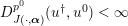 $D_{J(\cdot ,\unicode[STIX]{x1D736})}^{p^{0}}(u^{\dagger },u^{0})<\infty$
.
Proof. For
 $\unicode[STIX]{x1D6FF}=0$
we conclude
 $$\begin{eqnarray}F(Ku^{k},f)\leq D_{J(\cdot ,\unicode[STIX]{x1D736})}^{p^{k-1}}(u^{\dagger },u^{k-1})-D_{J(\cdot ,\unicode[STIX]{x1D736})}^{p^{k}}(u^{\dagger },u^{k})\end{eqnarray}$$
from Lemma 6.4. Summing up from
 $k=0$
to some
 $k=k^{\ast }$
therefore yields
 $$\begin{eqnarray}\mathop{\sum }_{k=0}^{k^{\ast }}F(Ku^{k},f)\leq D_{J(\cdot ,\unicode[STIX]{x1D736})}^{p^{0}}(u^{\dagger },u^{0})-D_{J(\cdot ,\unicode[STIX]{x1D736})}^{p^{k^{\ast }}}(u^{\dagger },u^{k^{\ast }})\leq D_{J(\cdot ,\unicode[STIX]{x1D736})}^{p^{0}}(u^{\dagger },u^{0})<\infty .\end{eqnarray}$$
Taking the limit
 $k^{\ast }\rightarrow \infty$
yields the assertion. ☐
Remark 6.6. Given the continuity of
 $F$
and
 $K\in {\mathcal{L}}({\mathcal{U}},{\mathcal{V}})$
, equation (6.5) already implies
 $$\begin{eqnarray}\displaystyle Ku^{k}\underset{\unicode[STIX]{x1D70F}_{{\mathcal{V}}}}{\longrightarrow }f, & & \displaystyle\end{eqnarray}$$
if
 $\unicode[STIX]{x1D70F}_{{\mathcal{V}}}$
is an appropriate topology on
 ${\mathcal{V}}$
related to
 $F$
.
Lemma 6.7. Suppose that after a finite number of iterations the
 $k^{\ast }$
th iterate of Algorithm 1 satisfies
 $Ku^{k^{\ast }}=f$
, for
 $u^{k^{\ast }}\in R(f,v^{k^{\ast }-1},\unicode[STIX]{x1D736})$
,
 $f\in {\mathcal{R}}_{K}(F)$
and
 $p^{0}\in {\mathcal{R}}(K^{\ast })$
. Then
 $u^{k^{\ast }}\in {\mathcal{S}}(f,\unicode[STIX]{x1D736})$
.
Proof. We know
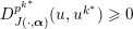 $D_{J(\cdot ,\unicode[STIX]{x1D736})}^{p^{k^{\ast }}}(u,u^{k^{\ast }})\geq 0$
for all
 $u\in {\mathcal{U}}$
and
 $u^{k^{\ast }}\in R_{I}(f,v^{k^{\ast }-1},\unicode[STIX]{x1D736})$
, since
 $J$
is convex; this in particular holds true for any
 $\hat{u} \in \{u\mid Ku=f\}$
. Hence, we observe
 $$\begin{eqnarray}\displaystyle J(u^{k^{\ast }}) & \leq & \displaystyle J(\hat{u} )-\langle p^{k^{\ast }},\hat{u} -u^{k^{\ast }}\rangle \nonumber\\ \displaystyle & = & \displaystyle J(\hat{u} )-\langle p^{0},\hat{u} -u^{k^{\ast }}\rangle +\mathop{\sum }_{n=1}^{k^{\ast }}\langle K^{\ast }\unicode[STIX]{x2202}_{x}F(Ku^{n},f),\hat{u} -u^{k^{\ast }}\rangle ,\nonumber\\ \displaystyle & \leq & \displaystyle J(\hat{u} )-\langle q^{0},\underbrace{K\hat{u} -Ku^{k^{\ast }}}_{=0}\rangle +\mathop{\sum }_{n=1}^{k^{\ast }}\langle \unicode[STIX]{x2202}_{x}F(Ku^{n},f),\vphantom{K^{\ast }\unicode[STIX]{x2202}_{x}F(Ku^{n},f),\hat{u} -u^{k^{\ast }}}\underbrace{K\hat{u} -Ku^{k^{\ast }}}_{=0}\vphantom{K^{\ast }\unicode[STIX]{x2202}_{x}F(Ku^{n},f),\hat{u} -u^{k^{\ast }}}\rangle ,\nonumber\\ \displaystyle & = & \displaystyle J(\hat{u} ),\nonumber\end{eqnarray}$$
for the substitution
 $p^{0}:=K^{\ast }q^{0}$
, which is possible since
 $p^{0}\in {\mathcal{R}}(K^{\ast })$
. Here we have made use of equation (6.3). Consequently, we conclude
 $u^{k^{\ast }}\in {\mathcal{S}}(f,\unicode[STIX]{x1D736})$
. ☐
In the limiting case
 $k^{\ast }\rightarrow \infty$
the selection is less clear: one cannot prove in general that the limit minimizes
 $J$
. To make this more apparent consider the case of a least-squares fidelity functional
 $F(Ku,f)={\textstyle \frac{1}{2}}\Vert Ku-f\Vert ^{2}$
, with the initial value being a minimizer of the regularization, i.e.
 $p^{0}=0$
. Then the estimate, as in the last proof (at arbitrary index
 $m$
) with
 $\hat{u} =u^{\dagger }$
, becomes
 $$\begin{eqnarray}\displaystyle J(u^{m}) & \leq & \displaystyle J(u^{\dagger })-\mathop{\sum }_{n=1}^{m}\langle K^{\ast }(f^{\unicode[STIX]{x1D6FF}}-Ku^{n}),\hat{u} -u^{m}\rangle \nonumber\\ \displaystyle & = & \displaystyle J(\hat{u} )-\mathop{\sum }_{n=1}^{m}\langle f^{\unicode[STIX]{x1D6FF}}-Ku^{n},f-Ku^{m}\rangle .\nonumber\end{eqnarray}$$
Using Young’s inequality and monotonicity of the residual (
 $\Vert Ku^{m}-f^{\unicode[STIX]{x1D6FF}}\Vert \leq \Vert Ku^{n}-f^{\unicode[STIX]{x1D6FF}}\Vert$
), we conclude that
 $$\begin{eqnarray}J(u^{m})\leq J(u^{\dagger })+\displaystyle \frac{3}{2}\mathop{\sum }_{n=1}^{m}\Vert Ku^{n}-f^{\unicode[STIX]{x1D6FF}}\Vert ^{2}+m\unicode[STIX]{x1D6FF}.\end{eqnarray}$$
Summing the estimate in the proof of the Fejér monotonicity, we further find
 $$\begin{eqnarray}\mathop{\sum }_{n=1}^{m}\Vert Ku^{n}-f^{\unicode[STIX]{x1D6FF}}\Vert ^{2}\leq D_{J}^{p^{0}}(u^{\dagger },u^{0})=J(u^{\dagger }).\end{eqnarray}$$
Thus, we find
 $$\begin{eqnarray}J(u^{k^{\ast }})\leq \displaystyle \frac{5}{2}J(u^{\dagger })+k^{\ast }\unicode[STIX]{x1D6FF}.\end{eqnarray}$$
Since for the discrepancy principle one can show that
 $k^{\ast }\unicode[STIX]{x1D6FF}^{2}\rightarrow 0$
in the limit
 $\unicode[STIX]{x1D6FF}\rightarrow 0$
(Osher et al.
Reference Osher, Burger, Goldfarb, Xu and Yin2005), the limit of the regularization has a functional value
 $J$
bounded by
 ${\textstyle \frac{5}{2}}J(u^{\dagger })$
. Using a more careful argument based on Young’s inequality, this upper bound can be decreased to
 $2J(u^{\dagger })$
but not to
 $J(u^{\dagger })$
. On the other hand this might be advantageous, since an estimate of
 $J(u^{k^{\ast }})$
smaller than
 $J(u^{\dagger })$
might mean a bias depending on
 $J$
, since the value of the regularization functional is actually underestimated. In the case of total variation, for example, this means that the contrast is underestimated by variational methods, which is improved by iterative regularization (Osher et al.
Reference Osher, Burger, Goldfarb, Xu and Yin2005). To conclude this section, we show numerical results of Bregman-iterative regularization in the context of deconvolution, which demonstrates the effect of total variation regularization.
(a) Image
 $u^{\dagger }\in \mathbb{R}^{400\times 300}$
of Pixel, a Gambian pouched rat. (b) Degraded and noisy version
 $f^{\unicode[STIX]{x1D6FF}}\in \mathbb{R}^{400\times 300}$
of the original image
 $u^{\dagger }$
. The degradation stems from a discretized version of the convolution (see (6.7)) with periodic boundary conditions and the convolution kernel depicted in the bottom left corner of (b). (c–h) Different iterates of Algorithm 1 for
 $F(Ku,f^{\unicode[STIX]{x1D6FF}})={\textstyle \frac{1}{2}}\Vert Ku-f^{\unicode[STIX]{x1D6FF}}\Vert _{L^{2}(\mathbb{R}^{2})}^{2}$
,
 $J(u,\unicode[STIX]{x1D6FC})=\unicode[STIX]{x1D6FC}\text{TV}(u)$
and
 $\unicode[STIX]{x1D6FC}=1/4$
. The 96th iterate visualized in (h) is the first that violates Definition 6.1, for
 $\unicode[STIX]{x1D702}=1$
and
 $\unicode[STIX]{x1D6FF}=5.95$
.

Example 6.8. We consider the inverse problem of the convolution operation, that is,
 $Ku=f$
with
 $$\begin{eqnarray}\displaystyle (Ku)(y):=\int _{\mathbb{R}^{2}}u(x)h(x-y)\,\text{d}x, & & \displaystyle\end{eqnarray}$$
which is therefore also known as deconvolution. Here,
 $h$
denotes the convolution kernel, that we assume to be known a priori. Since we cannot expect to know
 $f$
but just
 $f^{\unicode[STIX]{x1D6FF}}$
with
 $F(f,f^{\unicode[STIX]{x1D6FF}})\leq \unicode[STIX]{x1D6FF}$
, we need to approximate the inverse problem solution through regularization. In Figure 6.1 we can see selected iterates of Algorithm 1 for a single parameter
 $\unicode[STIX]{x1D6FC}=1/4$
, the data fidelity term
 $$\begin{eqnarray}F(Ku,f^{\unicode[STIX]{x1D6FF}})=\displaystyle \frac{1}{2}\Vert Ku-f^{\unicode[STIX]{x1D6FF}}\Vert _{L^{2}(\mathbb{R}^{2})}^{2},\end{eqnarray}$$
and the regularization functional
 $J(u,\unicode[STIX]{x1D6FC})=\unicode[STIX]{x1D6FC}\text{TV}(u)$
. The data
 $f^{\unicode[STIX]{x1D6FF}}=f+n$
are the sum of
 $f$
, created via a discretized version of the exact forward model (6.7), and noise
 $n\in {\mathcal{N}}(0,0.05)$
. For the particular example used here, the fidelity-noise-bound is
 $F(f,f^{\unicode[STIX]{x1D6FF}})=5.95$
. The inner variational regularization method is solved via the primal–dual hybrid gradient method (PDHGM): see Zhu and Chan (Reference Zhu and Chan2008), Pock, Cremers, Bischof and Chambolle (Reference Pock, Cremers, Bischof and Chambolle2009), Esser, Zhang and Chan (Reference Esser, Zhang and Chan2010) and Chambolle and Pock (Reference Chambolle and Pock2011, Reference Chambolle and Pock2016). We clearly observe the inverse scale-space nature of the Bregman iteration. The first iterate only contains features at a very coarse scale, and then ever more features at finer and finer scales are introduced throughout the course of the iteration.
Debiasing generalized eigenfunctions
We want to continue the analysis of the generalized eigenvalue problem introduced in Section 5.3. We have figured out that there is always a systematic bias of variational regularization methods for
 $$\begin{eqnarray}F(Ku,f^{\unicode[STIX]{x1D6FF}})=\displaystyle \frac{1}{2}\Vert Ku-f^{\unicode[STIX]{x1D6FF}}\Vert _{L^{2}(\unicode[STIX]{x1D6F4})}^{2},\end{eqnarray}$$
i.e.
 $\unicode[STIX]{x1D706}<1$
in (5.11) for
 $f^{\unicode[STIX]{x1D6FF}}=v_{\unicode[STIX]{x1D70E}}$
. Benning (Reference Benning2011) showed that this systematic bias can be corrected with the help of Bregman iterations in the case of scalar
 $\unicode[STIX]{x1D736}=\unicode[STIX]{x1D6FC}$
and
 $J$
with
 $\unicode[STIX]{x2202}J(cu,\unicode[STIX]{x1D6FC})=\unicode[STIX]{x1D6FC}\unicode[STIX]{x2202}J(u)$
. Assume that
 $\unicode[STIX]{x1D6FC}$
is chosen such that
 $u^{k}=0$
for all
 $k<k^{\ast }-1$
, and
 $u^{k^{\ast }-1}=(1-\unicode[STIX]{x1D6FC})\unicode[STIX]{x1D70E}^{-1}u_{\unicode[STIX]{x1D70E}}$
for some
 $k^{\ast }\in \mathbb{N}$
. Then we can easily conclude from (5.4) and (6.4) that
 $u^{k^{\ast }}$
has to satisfy
 $$\begin{eqnarray}\displaystyle \frac{1}{\unicode[STIX]{x1D6FC}}\biggl(\unicode[STIX]{x1D706}-\displaystyle \frac{1-\unicode[STIX]{x1D6FC}}{\unicode[STIX]{x1D70E}}\biggr)K^{\ast }Ku^{k^{\ast }}\in \unicode[STIX]{x2202}J(\unicode[STIX]{x1D706}u^{k^{\ast }}).\end{eqnarray}$$
We easily calculate that the above equation simplifies to the singular vector condition (5.14) for the choice
 $\unicode[STIX]{x1D706}=1/\unicode[STIX]{x1D70E}$
. Consequently,
 $u^{k^{\ast }}=R(f^{\unicode[STIX]{x1D6FF}},\unicode[STIX]{x1D6FC})=u_{\unicode[STIX]{x1D70E}}/\unicode[STIX]{x1D70E}$
, and we have corrected for the bias of the previous iterate.
These computations demonstrate that Bregman iterations correct for the systematic bias of variational regularization reconstructions of generalized singular vectors for one-homogeneous regularization functionals
 $J$
. However, the phenomenon is not limited to singular vectors. The following numerical toy example shows that the average reconstruction bias can be significantly reduced with the help of Bregman iterations. Assume the following set-up. Our forward model
 $K\in \mathbb{R}^{m\times n}$
, for
 $m=128$
and
 $n=512$
, is a matrix with its entries drawn randomly from
 ${\mathcal{N}}(0,1)$
. We define a sparse vector
 $u^{\dagger }\in \mathbb{R}^{n}$
with nine non-zero entries, drawn randomly from
 ${\mathcal{N}}(0,1)$
, and set
 $f=Ku^{\dagger }$
. Subsequently, we create one hundred instances of noisy data via
 $f_{j}^{\unicode[STIX]{x1D6FF}}:=f+n_{j}$
, for
 $n\in {\mathcal{N}}(0,0.5)$
and
 $j\in \{1,\ldots ,100\}$
. We now compute reconstructions for each of the one hundred instances with the following two regularization methods:
 $$\begin{eqnarray}\displaystyle R_{\text{Morozov}}(f_{j}^{\unicode[STIX]{x1D6FF}},\unicode[STIX]{x1D6FF}_{j})=\underset{u\in \mathbb{R}^{n}}{\operatorname{argmin}}\,\{\Vert u\Vert _{1}\quad \text{subject to }\Vert Ku-f_{j}^{\unicode[STIX]{x1D6FF}}\Vert _{2}\leq \unicode[STIX]{x1D6FF}_{j}\}, & & \displaystyle\end{eqnarray}$$
and
 $$\begin{eqnarray}\displaystyle & & \displaystyle R_{\text{Bregman}}(f_{j}^{\unicode[STIX]{x1D6FF}},\{u_{j}^{n}\}_{n=1}^{k-1},\unicode[STIX]{x1D6FC})\nonumber\\ \displaystyle & & \displaystyle \quad =\underset{u\in \mathbb{R}^{n}}{\operatorname{argmin}}\,\biggl\{\displaystyle \frac{1}{2}\biggl\|Ku-\biggl(kf^{\unicode[STIX]{x1D6FF}}-\mathop{\sum }_{n=1}^{k-1}Ku_{j}^{n}\biggr)\biggr\|_{2}^{2}+\unicode[STIX]{x1D6FC}\Vert u\Vert _{1}\biggr\},\end{eqnarray}$$
for
 $$\begin{eqnarray}\displaystyle u_{j}^{\text{Morozov}} & \in & \displaystyle R_{\text{Morozov}}(f_{j}^{\unicode[STIX]{x1D6FF}},\unicode[STIX]{x1D6FF}_{j}),\nonumber\\ \displaystyle \unicode[STIX]{x1D6FF}_{j} & := & \displaystyle \displaystyle \frac{1}{2}\Vert Ku^{\dagger }-f_{j}^{\unicode[STIX]{x1D6FF}}\Vert _{2}^{2},\nonumber\\ \displaystyle u_{j}^{\text{Bregman}} & \in & \displaystyle R_{\text{Bregman}}(f_{j}^{\unicode[STIX]{x1D6FF}},\{u_{j}^{n}\}_{n=1}^{k^{\ast }-1},\unicode[STIX]{x1D6FC}),\nonumber\end{eqnarray}$$
and
 $k^{\ast }$
chosen according to Definition 6.1 for
 $\unicode[STIX]{x1D702}=1$
and
 $\unicode[STIX]{x1D6FF}=\unicode[STIX]{x1D6FF}_{j}$
. We then compute the average absolute bias and the standard deviation of the reconstructions, that is, we compute
 $$\begin{eqnarray}\displaystyle \biggl|u^{\dagger }-\displaystyle \frac{1}{100}\mathop{\sum }_{j=1}^{100}\hat{u} _{j}\biggr|\quad \text{and}\quad \sqrt{\displaystyle \frac{1}{99}\mathop{\sum }_{j=1}^{100}\biggl(\hat{u} _{j}-\displaystyle \frac{1}{100}\mathop{\sum }_{j=1}^{100}\hat{u} _{j}\biggr)^{2}} & & \displaystyle\end{eqnarray}$$
for
 $\hat{u} _{j}\in \{u_{j}^{\text{Morozov}},u_{j}^{\text{Bregman}}\}$
. Both average absolute bias and standard deviation are visualized for each of the
 $n=512$
coefficients in Figure 6.2. We clearly observe that with similar standard deviation, the average absolute bias is significantly reduced by the Bregman iteration in comparison to the Morozov regularization model.
Equation (6.10) for the compressed sensing toy example in Section 6.1. The blue circles represent the standard deviation and average absolute bias values for all coefficients recovered with (6.8). The red circles show the same but for quantities for all coefficients recovered with (6.9). It becomes evident that for this example the average bias is significantly reduced, while the standard deviation of the reconstructed coefficients is comparable.

6.2 Linearized Bregman iteration
As the name suggests, the linearized Bregman iteration can be derived from Algorithm 1 by replacing the term
 $F(Ku^{k},f^{\unicode[STIX]{x1D6FF}})$
with its linearization
 $$\begin{eqnarray}F(Ku^{k},f^{\unicode[STIX]{x1D6FF}})\approx F(Ku^{k-1},f^{\unicode[STIX]{x1D6FF}})+\langle \unicode[STIX]{x2202}_{x}F(Ku^{k-1},f^{\unicode[STIX]{x1D6FF}}),Ku^{k}-Ku^{k-1}\rangle .\end{eqnarray}$$
Hence, if we replace
 $F(Ku^{k},f^{\unicode[STIX]{x1D6FF}})$
in Algorithm 1 with this linearization multiplied by some constant
 $\unicode[STIX]{x1D70F}>0$
, we obtain
 $$\begin{eqnarray}\displaystyle & & \displaystyle R_{I}(f^{\unicode[STIX]{x1D6FF}},v^{k-1},\unicode[STIX]{x1D736})\nonumber\\ \displaystyle & & \displaystyle \quad =\underset{u\in {\mathcal{U}}}{\operatorname{argmin}}\,\{\unicode[STIX]{x1D70F}(F(Ku^{k-1},f^{\unicode[STIX]{x1D6FF}})+\langle \unicode[STIX]{x2202}_{x}F(Ku^{k-1},f^{\unicode[STIX]{x1D6FF}}),Ku^{k}-Ku^{k-1}\rangle )\nonumber\\ \displaystyle & & \displaystyle \qquad +\,D_{J(\cdot ,\unicode[STIX]{x1D6FC})}^{p^{k-1}}(u,u^{k-1})\},\nonumber\\ \displaystyle & & \displaystyle \quad =\underset{u\in {\mathcal{U}}}{\operatorname{argmin}}\,\{\unicode[STIX]{x1D70F}\langle \unicode[STIX]{x2202}_{x}F(Ku^{k-1},f^{\unicode[STIX]{x1D6FF}}),Ku^{k}-Ku^{k-1}\rangle +D_{J(\cdot ,\unicode[STIX]{x1D6FC})}^{p^{k-1}}(u,u^{k-1})\},\nonumber\\ \displaystyle & & \displaystyle u^{k}\in R_{I}(f^{\unicode[STIX]{x1D6FF}},v^{k-1},\unicode[STIX]{x1D736})\nonumber\\ \displaystyle & & \displaystyle p^{k}=p^{k-1}-\unicode[STIX]{x1D70F}K^{\ast }\unicode[STIX]{x2202}_{x}F(Ku^{k-1},f^{\unicode[STIX]{x1D6FF}}),\nonumber\end{eqnarray}$$
for
 $\unicode[STIX]{x1D736}=(\unicode[STIX]{x1D70F},\unicode[STIX]{x1D6FC})$
and
 $v^{k-1}:=(u^{k},p^{k})$
for all
 $k\in \mathbb{N}$
. These equations are summarized in Algorithm 2.
The linearized Bregman iteration is a generalization of the Landweber regularization (Landweber Reference Landweber1951) for the choices
 $$\begin{eqnarray}F(Ku,f^{\unicode[STIX]{x1D6FF}})=\displaystyle \frac{1}{2}\Vert Ku-f^{\unicode[STIX]{x1D6FF}}\Vert _{L^{2}(\unicode[STIX]{x1D6F4})}^{2}\quad \text{and}\quad J(u,\unicode[STIX]{x1D6FC})=\displaystyle \frac{\unicode[STIX]{x1D6FC}}{2}\Vert u\Vert _{L^{2}(\unicode[STIX]{x1D6FA})}^{2},\end{eqnarray}$$
for some signal domains
 $\unicode[STIX]{x1D6FA}$
and
 $\unicode[STIX]{x1D6F4}$
. It is also a generalization of the mirror descent algorithm proposed in Nemirovskii and Yudin (Reference Nemirovskii and Yudin1983), where
 $J(\cdot ,\unicode[STIX]{x1D6FC})$
is a Legendre functional in the sense of Definition 5.11. This connection for convex, differentiable
 $F$
and strongly convex and differentiable
 $J(\cdot ,\unicode[STIX]{x1D6FC})$
was made in Beck and Teboulle (Reference Beck and Teboulle2003). The extension to subdifferentiable convex
 $J(\cdot ,\unicode[STIX]{x1D6FC})$
was first proposed in Darbon and Osher (Reference Darbon and Osher2007) and has since been studied extensively (Yin, Osher, Goldfarb and Darbon Reference Yin, Osher, Goldfarb and Darbon2008, Cai, Osher and Shen Reference Cai, Osher and Shen2009b
, Cai, Osher and Shen Reference Cai, Osher and Shen2009a
, Yin Reference Yin2010).

As in Remark 6.2, we can rewrite the dual update of the linearized Bregman iteration as
 $$\begin{eqnarray}\displaystyle p^{k}=p^{0}-\mathop{\sum }_{n=0}^{k-1}K^{\ast }\unicode[STIX]{x2202}_{x}F(Ku^{n},f^{\unicode[STIX]{x1D6FF}}), & & \displaystyle\end{eqnarray}$$
and the primal update as
 $$\begin{eqnarray}\displaystyle & & \displaystyle R_{I}(f^{\unicode[STIX]{x1D6FF}},\{u^{n}\}_{n=0}^{k-1},p^{0},\unicode[STIX]{x1D6FC})\nonumber\\ \displaystyle & & \displaystyle \quad =\underset{u\in {\mathcal{U}}}{\operatorname{argmin}}\,\biggl\{J(u,\unicode[STIX]{x1D6FC})-\langle p^{0}-\mathop{\sum }_{n=0}^{k-1}K^{\ast }\unicode[STIX]{x2202}_{x}F(Ku^{n},f^{\unicode[STIX]{x1D6FF}}),u\rangle \biggr\}.\end{eqnarray}$$
In order to carry out a convergence analysis similar to the analysis for the standard Bregman iteration, we define the surrogate functional
 $$\begin{eqnarray}\displaystyle J_{\unicode[STIX]{x1D70F}}(u,\unicode[STIX]{x1D6FC}):=J(u,\unicode[STIX]{x1D6FC})-\unicode[STIX]{x1D70F}F(Ku,f^{\unicode[STIX]{x1D6FF}}). & & \displaystyle\end{eqnarray}$$
We further assume for the remainder of this section that
 $J$
and
 $\unicode[STIX]{x1D70F}$
are chosen such that
 $J_{\unicode[STIX]{x1D70F}}$
is convex. In practice, this requires strong convexity properties of
 $J$
, which can simply be established by adding a sufficiently strongly convex functional to the original choice of
 $J$
.
Example 6.9. Let
 $$\begin{eqnarray}K\in {\mathcal{L}}(L^{2}(\unicode[STIX]{x1D6FA}),L^{2}(\unicode[STIX]{x1D6F4})),\quad F(Ku,f^{\unicode[STIX]{x1D6FF}})=\displaystyle \frac{1}{2}\Vert Ku-f^{\unicode[STIX]{x1D6FF}}\Vert _{L^{2}(\unicode[STIX]{x1D6F4})}^{2},\end{eqnarray}$$
for domains
 $\unicode[STIX]{x1D6FA}\subset \mathbb{R}^{n}$
and
 $\unicode[STIX]{x1D6F4}\subset \mathbb{R}^{m}$
, and let
 $J_{1}$
be a proper, lower semicontinuous and convex functional. Then the functional
 $$\begin{eqnarray}J_{\unicode[STIX]{x1D70F}}(u,\unicode[STIX]{x1D6FC}):=J(u,\unicode[STIX]{x1D6FC})-\displaystyle \frac{\unicode[STIX]{x1D70F}}{2}\Vert Ku-f^{\unicode[STIX]{x1D6FF}}\Vert _{L^{2}(\unicode[STIX]{x1D6F4})}^{2}\end{eqnarray}$$
is convex for the choices
 $$\begin{eqnarray}J(u,\unicode[STIX]{x1D6FC}):=\displaystyle \frac{1}{2}\Vert u\Vert _{L^{2}(\unicode[STIX]{x1D6FA})}^{2}+J_{1}(u)\quad \text{and}\quad \unicode[STIX]{x1D70F}<\displaystyle \frac{1}{\Vert K\Vert _{{\mathcal{L}}(L^{2}(\unicode[STIX]{x1D6FA}),L^{2}(\unicode[STIX]{x1D6F4}))}^{2}}.\end{eqnarray}$$
As for the Bregman iteration analysis, we start with a statement about the monotonic decrease of data fidelity.
Corollary 6.10 (monotonic decrease of data fidelity).
Suppose that
 $u^{0}$
satisfies
 $F(Ku^{0},f^{\unicode[STIX]{x1D6FF}})<\infty$
. Then the iterates of Algorithm 2 satisfy
 $$\begin{eqnarray}\displaystyle F(Ku^{k+1},f^{\unicode[STIX]{x1D6FF}})+\displaystyle \frac{1}{\unicode[STIX]{x1D70F}}D_{J_{\unicode[STIX]{x1D70F}}(\cdot ,\unicode[STIX]{x1D6FC})}^{q^{k}}(u^{k+1},u^{k})\leq F(Ku^{k+1},f^{\unicode[STIX]{x1D6FF}}) & & \displaystyle\end{eqnarray}$$
and
 $$\begin{eqnarray}\lim _{k\rightarrow \infty }D_{J_{\unicode[STIX]{x1D70F}}(\cdot ,\unicode[STIX]{x1D6FC})}^{q^{k}}(u^{k+1},u^{k})=0,\end{eqnarray}$$
for
 $u^{k}\in R(f^{\unicode[STIX]{x1D6FF}},v^{k-1},\unicode[STIX]{x1D736})$
and
 $q^{k}\in \unicode[STIX]{x2202}J_{\unicode[STIX]{x1D70F}}(u^{k},\unicode[STIX]{x1D6FC})$
.
Proof. First of all we emphasize that
 $$\begin{eqnarray}\langle r^{k-1},u^{k}-u^{k-1}\rangle =\langle K^{\ast }\unicode[STIX]{x2202}_{x}F(Ku^{k-1},f^{\unicode[STIX]{x1D6FF}}),u^{k}-u^{k-1}\rangle\end{eqnarray}$$
can be written as
 $$\begin{eqnarray}\displaystyle & & \displaystyle \langle K^{\ast }\unicode[STIX]{x2202}_{x}F(Ku^{k-1},f^{\unicode[STIX]{x1D6FF}}),u^{k}-u^{k-1}\rangle \nonumber\\ \displaystyle & & \displaystyle \quad =F(Ku^{k},f^{\unicode[STIX]{x1D6FF}})-F(Ku^{k-1},f^{\unicode[STIX]{x1D6FF}})-D_{F(K\cdot ,f^{\unicode[STIX]{x1D6FF}})}^{}(u^{k},u^{k-1}),\nonumber\end{eqnarray}$$
for all
 $k\in \mathbb{N}$
. Hence, the (primal) update of the linearized Bregman iteration can be rewritten as
 $$\begin{eqnarray}\displaystyle & & \displaystyle R_{I}(f^{\unicode[STIX]{x1D6FF}},v^{k-1},\unicode[STIX]{x1D736})\nonumber\\ \displaystyle & & \displaystyle \quad =\underset{u\in {\mathcal{U}}}{\operatorname{argmin}}\,\{\unicode[STIX]{x1D70F}(F(Ku^{k},f^{\unicode[STIX]{x1D6FF}})-F(Ku^{k-1},f^{\unicode[STIX]{x1D6FF}}))+D_{J_{\unicode[STIX]{x1D70F}}(\cdot ,\unicode[STIX]{x1D6FC})}^{q^{k-1}}(u^{k},u^{k-1})\},\nonumber\end{eqnarray}$$
for
 $$\begin{eqnarray}q^{k-1}=p^{k-1}-\unicode[STIX]{x1D70F}K^{\ast }\unicode[STIX]{x2202}_{x}F(Ku^{k-1},f^{\unicode[STIX]{x1D6FF}})\in \unicode[STIX]{x2202}J_{\unicode[STIX]{x1D70F}}(u^{k-1},\unicode[STIX]{x1D6FC}),\quad p^{k-1}\in \unicode[STIX]{x2202}J(u^{k-1},\unicode[STIX]{x1D6FC}).\end{eqnarray}$$
Hence, we conclude
 $$\begin{eqnarray}\displaystyle & & \displaystyle \unicode[STIX]{x1D70F}(F(Ku^{k},f^{\unicode[STIX]{x1D6FF}})-F(Ku^{k-1},f^{\unicode[STIX]{x1D6FF}}))+D_{J_{\unicode[STIX]{x1D70F}}(\cdot ,\unicode[STIX]{x1D6FC})}^{q^{k-1}}(u^{k},u^{k-1})\nonumber\\ \displaystyle & & \displaystyle \quad \leq \underbrace{\unicode[STIX]{x1D70F}(F(Ku^{k-1},f^{\unicode[STIX]{x1D6FF}})-F(Ku^{k-1},f^{\unicode[STIX]{x1D6FF}}))}_{=0}+\underbrace{D_{J_{\unicode[STIX]{x1D70F}}(\cdot ,\unicode[STIX]{x1D6FC})}^{q^{k-1}}(u^{k-1},u^{k-1})}_{=0},\nonumber\end{eqnarray}$$
and thus equation (6.14). In the same fashion as in the proof of Corollary 6.3, we further conclude
 $\lim _{k\rightarrow \infty }D_{J_{\unicode[STIX]{x1D70F}}(\cdot ,\unicode[STIX]{x1D6FC})}^{q^{k}}(u^{k+1},u^{k})=0$
. ☐
As in the case of the standard Bregman iteration, the linearized Bregman iteration also satisfies Fejér monotonicity when the discrepancy principle is not violated.
Lemma 6.11 (Fejér monotonicity of Algorithm 2).
Let
 $f\in {\mathcal{R}}_{F}(K)$
,
 $u^{\dagger }\in {\mathcal{S}}(f,\unicode[STIX]{x1D6FC})$
and let
 $f^{\unicode[STIX]{x1D6FF}}\in {\mathcal{V}}$
with
 $F(f,f^{\unicode[STIX]{x1D6FF}})\leq \unicode[STIX]{x1D6FF}$
. We further assume that the iterates of Algorithm 2 satisfy Definition 6.1 for
 $\unicode[STIX]{x1D702}=1$
. Then the iterates also satisfy the strict Fejér monotonicity
 $$\begin{eqnarray}D_{J_{\unicode[STIX]{x1D70F}}(\cdot ,\unicode[STIX]{x1D6FC})}^{q^{k}}(u^{\dagger },u^{k})<D_{J_{\unicode[STIX]{x1D70F}}(\cdot ,\unicode[STIX]{x1D6FC})}^{q^{k-1}}(u^{\dagger },u^{k-1}),\end{eqnarray}$$
for all
 $u^{k}\in R(f^{\unicode[STIX]{x1D6FF}},v^{k-1},\unicode[STIX]{x1D736})$
and
 $q^{k}\in \unicode[STIX]{x2202}J_{\unicode[STIX]{x1D70F}}(u^{k},\unicode[STIX]{x1D6FC})$
, for all
 $k\leq k^{\ast }$
.
Proof. Through straightforward computations we obtain
 $$\begin{eqnarray}\displaystyle & & \displaystyle D_{J_{\unicode[STIX]{x1D70F}}(\cdot ,\unicode[STIX]{x1D6FC})}^{q^{k}}(u^{\dagger },u^{k})-D_{J_{\unicode[STIX]{x1D70F}}(\cdot ,\unicode[STIX]{x1D6FC})}^{q^{k-1}}(u^{\dagger },u^{k-1})\nonumber\\ \displaystyle & & \displaystyle \quad =\underbrace{-D_{J_{\unicode[STIX]{x1D70F}}(\cdot ,\unicode[STIX]{x1D6FC})}^{q^{k-1}}(u^{k},u^{k-1})}_{{<}0}-\langle q^{k}-q^{k-1},u^{\dagger }-u^{k}\rangle \nonumber\\ \displaystyle & & \displaystyle \quad \leq \langle p^{k-1}-p^{k}+\unicode[STIX]{x1D70F}K^{\ast }(\unicode[STIX]{x2202}_{x}F(Ku^{k},f^{\unicode[STIX]{x1D6FF}})-\unicode[STIX]{x2202}_{x}F(Ku^{k-1},f^{\unicode[STIX]{x1D6FF}})),u^{\dagger }-u^{k}\rangle \nonumber\\ \displaystyle & & \displaystyle \quad =\unicode[STIX]{x1D70F}\langle K^{\ast }\unicode[STIX]{x2202}_{x}F(Ku^{k},f^{\unicode[STIX]{x1D6FF}}),u^{\dagger }-u^{k}\rangle \nonumber\\ \displaystyle & & \displaystyle \quad \leq \unicode[STIX]{x1D70F}(\unicode[STIX]{x1D6FF}-F(Ku^{k},f^{\unicode[STIX]{x1D6FF}}))\nonumber\\ \displaystyle & & \displaystyle \quad <0\nonumber\end{eqnarray}$$
for
 $k\leq k^{\ast }$
, where we have made use of the convexity of
 $F$
in its first argument, and
 $F(Ku^{\dagger },f^{\unicode[STIX]{x1D6FF}})\leq \unicode[STIX]{x1D6FF}$
. ☐
In analogy to Corollary 6.5, we can show the same result for the linearized Bregman iteration.
Corollary 6.12. Let
 $f\in {\mathcal{R}}_{F}(K)$
and
 $u^{\dagger }\in {\mathcal{S}}(f,\unicode[STIX]{x1D6FC})$
. Then the iterates of Algorithm 2 satisfy (6.5), for
 $\unicode[STIX]{x1D6FF}=0$
(and thus
 $f^{\unicode[STIX]{x1D6FF}}=f$
) and
 $u^{0}$
(with
 $q^{0}\in \unicode[STIX]{x2202}J_{\unicode[STIX]{x1D70F}}(u^{0},\unicode[STIX]{x1D6FC})$
) chosen such that
 $D_{J_{\unicode[STIX]{x1D70F}}(\cdot ,\unicode[STIX]{x1D6FC})}^{q^{0}}(u^{\dagger },u^{0})<\infty$
.
Proof. The proof follows exactly the same steps as the proof of Corollary 6.5. ☐
As in the case of Bregman iteration, Remark 6.6 follows from this result.
The following result guarantees convergence to a solution in
 ${\mathcal{S}}(f,\unicode[STIX]{x1D6FC})$
when
 $Ku^{k^{\ast }}=f$
is satisfied after a finite number
 $k^{\ast }$
of iterations of Algorithm 2.
Lemma 6.13. Suppose that after a finite number of iterations the
 $k^{\ast }$
th iterate of Algorithm 2 satisfies
 $Ku^{k^{\ast }}=f$
, for
 $u^{k^{\ast }}=R(f,\unicode[STIX]{x1D736})$
,
 $f\in {\mathcal{R}}_{K}(F)$
and
 $p^{0}\in {\mathcal{R}}(K^{\ast })$
. Then
 $u^{k^{\ast }}\in {\mathcal{S}}(f,\unicode[STIX]{x1D6FC})$
.
Proof. The proof is almost identical to the proof of Lemma 6.7; the only difference is that we use (6.11) instead of (6.3). ☐
Remark 6.14. Note that the statements of Lemmas 6.7 and 6.13 look identical, but one needs to remember that the underlying functionals
 $J$
will most likely not be. This is due to the fact that for the linearized Bregman iteration additional terms have to be added in order to also make
 $J_{\unicode[STIX]{x1D70F}}$
convex.
(a) Image
 $u^{\dagger }\in \mathbb{R}^{400\times 300}$
of Pixel the Gambian pouched rat, introduced in Figure 6.1(a). (b) The same degraded and noisy version
 $f^{\unicode[STIX]{x1D6FF}}\in \mathbb{R}^{400\times 300}$
together with the convolution kernel
 $h$
as shown in Figure 6.1(b). (c–h) Different iterates of Algorithm 2 for
 $F(Ku,f^{\unicode[STIX]{x1D6FF}})={\textstyle \frac{1}{2}}\Vert Ku-f^{\unicode[STIX]{x1D6FF}}\Vert _{L^{2}(\mathbb{R}^{2})}^{2}$
,
 $J(u,\unicode[STIX]{x1D6FC})={\textstyle \frac{1}{2}}\Vert u\Vert _{L^{2}(\mathbb{R}^{2})}^{2}+\unicode[STIX]{x1D6FC}\text{TV}(u)$
and
 $\unicode[STIX]{x1D6FC}=1/4$
. The 128th iterate visualized in (h) is the first that violates Definition 6.1, for
 $\unicode[STIX]{x1D6FF}=5.95$
.

We conclude this section with numerical results for the same deconvolution example introduced in Example 6.8. We observe that with the same choice of regularization parameter and the same initialization, Algorithm 2 requires more iterations in order to converge to a solution that violates the discrepancy principle with the same error bound. See Figure 6.3. On the other hand, the variational subproblems are computationally cheaper to solve compared to the standard Bregman iteration case, at least with the (accelerated) PDHGM used for this example.
6.3 Coupled and modified Bregman iterations
The Bregman iteration (as well as its linearized variant) leave some freedom for modifications. One obvious modification is the choice of the subgradient
 $p^{k-1}$
. The update from the optimality condition is of course the obvious one and particularly suitable for a convergence proof. However, one may use different ways to determine a subgradient
 $p^{k}$
from
 $u^{k}$
. As an example one may solve some variational problem
 $$\begin{eqnarray}p^{k}\in \underset{p}{\operatorname{argmin}}\,\{H(p,p^{k-1})\mid p\in \unicode[STIX]{x2202}J(u^{k},\boldsymbol{\unicode[STIX]{x1D6FC}})\},\end{eqnarray}$$
with a convex functional
 $H$
. In the case of
 $\ell ^{1}$
-minimization one might choose
 $H(p,p^{k-1})=\Vert p\Vert _{2}$
, which yields the minimal subgradient, that is, again choosing sign
 $_{0}(p)$
(the single-valued version with sign
 $_{0}(0)=0$
) in the case of a multivalued sign.
Another option for choosing subgradients has been investigated by Moeller et al. (Reference Moeller, Brinkmann, Burger and Seybold2014), when one solves joint reconstruction problems for multiple unknowns
 $u_{1},\ldots ,u_{M}$
. Moeller et al. (Reference Moeller, Brinkmann, Burger and Seybold2014) proposed and analysed a coupled Bregman iteration, which is based on choosing a new subgradient for the Bregman iteration in the
 $i$
th image
 $u_{i}$
from a linear combination of the subgradients in the other channels. In this way a joint subgradient for all the channels is approximated, which means a structural joint sparsity in the case of the
 $\ell ^{1}$
-norm or joint edge information in the total variation case. Rasch et al. (Reference Rasch, Brinkmann and Burger2018) have investigated an infimal convolution version of the coupled Bregman iteration for an application to PET-MR imaging.
7 Bias and scales
Our earlier arguments relating to eigenfunctions demonstrate that bias and scale are closely related (at least when interpreting scale in terms of eigenfunctions and eigenvalues). The bias of variational regularization methods is larger on small-scale features. Thus, debiasing and multiscale aspects in regularization methods appear to be closely related, as has been worked out very recently. We discuss these ideas below.
7.1 Inverse scale space
For regularization functionals of the form
 $J(u,\unicode[STIX]{x1D736})=\unicode[STIX]{x1D6FC}J_{1}(u)$
we can write the dual Bregman iteration update as
 $$\begin{eqnarray}\displaystyle \frac{p^{k}-p^{k-1}}{\unicode[STIX]{x1D6E5}t}=-K^{\ast }\unicode[STIX]{x2202}_{x}F(Ku^{k},f^{\unicode[STIX]{x1D6FF}})\end{eqnarray}$$
for
 $\unicode[STIX]{x1D6E5}t:=1/\unicode[STIX]{x1D6FC}$
and
 $p^{k}\in \unicode[STIX]{x2202}J_{1}(u^{k})$
, for all
 $k\in \mathbb{N}$
. Thus, taking the limit
 $\unicode[STIX]{x1D6FC}\rightarrow \infty$
, so that
 $\unicode[STIX]{x1D6E5}t\rightarrow 0$
, yields the following time-continuous formulation of the Bregman iteration, also known as the inverse scale space flow (Burger, Osher, Xu and Gilboa Reference Burger, Osher, Xu, Gilboa and Paragios2005, Burger et al.
Reference Burger, Gilboa, Osher and Xu2006, Burger, Frick, Osher and Scherzer Reference Burger, Frick, Osher and Scherzer2007a
),
 $$\begin{eqnarray}\displaystyle \unicode[STIX]{x2202}_{t}p(t)=-K^{\ast }\unicode[STIX]{x2202}_{x}F(Ku(t),f^{\unicode[STIX]{x1D6FF}}), & & \displaystyle\end{eqnarray}$$
for
 $p(t)\in \unicode[STIX]{x2202}J_{1}(u(t))$
.
For many typical choices of regularization functionals
 $J_{1}$
, it is difficult to numerically compute solutions of (7.1), with the
 $\ell ^{1}$
-norm and in general any polyhedral regularization functional being the exception (Burger, Moeller, Benning and Osher Reference Burger, Moeller, Benning and Osher2013c
, Moeller Reference Moeller2012, Moeller and Burger Reference Moeller and Burger2013). Nevertheless, (7.1) is very useful for studying theoretical properties of iterative regularizations in the limiting case.
Unsurprisingly, it is straightforward to carry out an eigenanalysis similar to the one discussed in Sections 5.3 and 6.1 for the regularization operator
 $R(f^{\unicode[STIX]{x1D6FF}},t)=u(t)$
with
 $u(t)$
satisfying (7.1) for
 $F(Ku,f^{\unicode[STIX]{x1D6FF}})=G(Ku-f^{\unicode[STIX]{x1D6FF}})$
. The following result is a generalization of Benning and Burger (Reference Benning and Burger2013, Theorem 9).
Theorem 7.1. Let
 $(u_{\unicode[STIX]{x1D70E}},v_{\unicode[STIX]{x1D70E}})$
be a pair of generalized singular vectors with singular value
 $\unicode[STIX]{x1D70E}$
,
 $f=v_{\unicode[STIX]{x1D70E}}$
and suppose
 $J_{1}$
is (absolutely) one-homogeneous, that is,
 $J_{1}(cu)=|c|J_{1}(u)$
for all
 $c\in \mathbb{R}$
. Then
 $0\in R(v_{\unicode[STIX]{x1D70E}},t)$
for
 $0\leq t<t_{\ast }$
and
 $$\begin{eqnarray}\displaystyle \frac{1}{\unicode[STIX]{x1D70E}}u_{\unicode[STIX]{x1D70E}}\in R(v_{\unicode[STIX]{x1D70E}},t)\end{eqnarray}$$
for
 $t\geq t_{\ast }=1$
.
Proof. First we verify
 $0\in R(v_{\unicode[STIX]{x1D70E}},t)$
for
 $0\in [0,t_{\ast })$
. From (5.14) and the absolute one-homogeneity of
 $J_{1}$
, we observe
 $J_{1}(u_{\unicode[STIX]{x1D70E}})=\langle G^{\prime }(v_{\unicode[STIX]{x1D70E}}),Ku_{\unicode[STIX]{x1D70E}}\rangle$
. We further see from the definition of the subdifferential that
 $t\leq 1=\langle G^{\prime }(v_{\unicode[STIX]{x1D70E}}),Ku_{\unicode[STIX]{x1D70E}}\rangle /J_{1}(u_{\unicode[STIX]{x1D70E}})$
implies
 $p(t):=tK^{\ast }G^{\prime }(v_{\unicode[STIX]{x1D70E}})\in \unicode[STIX]{x2202}J_{1}(0)$
. Since
 $\unicode[STIX]{x2202}_{t}p(t)=K^{\ast }G^{\prime }(v_{\unicode[STIX]{x1D70E}})$
and
 $p(0)=0$
, we have shown that
 $u(t)=0$
is a solution of (7.1).
For
 $t\geq t_{\ast }$
a continuous extension of
 $p(t)$
is
 $$\begin{eqnarray}p(t)=p(t_{\ast })+(t_{\ast }-t)K^{\ast }G^{\prime }(Ku(t)-v_{\unicode[STIX]{x1D70E}}).\end{eqnarray}$$
We immediately see that
 $u(t)=u_{\unicode[STIX]{x1D70E}}/\unicode[STIX]{x1D70E}$
is a solution for
 $t\geq t_{\ast }$
, since
 $p(t_{\ast })=t_{\ast }K^{\ast }G^{\prime }(v_{\unicode[STIX]{x1D70E}})\in \unicode[STIX]{x2202}J_{1}(u_{\unicode[STIX]{x1D70E}}/\unicode[STIX]{x1D70E})$
and
 $\unicode[STIX]{x2202}_{t}p(t)=0$
. ☐
Hence, the inverse scale space reconstruction also has no bias (for input data
 $v_{\unicode[STIX]{x1D70E}}$
satisfying (5.14)), compared to the variational regularization method.
A similar result can be derived even in the case of noisy data
 $f^{\unicode[STIX]{x1D6FF}}=v_{\unicode[STIX]{x1D70E}}+n$
, where
 $n$
is an error term that satisfies the specific source condition
 $$\begin{eqnarray}\unicode[STIX]{x1D707}K^{\ast }G^{\prime }(v_{\unicode[STIX]{x1D70E}})+\unicode[STIX]{x1D702}K^{\ast }n\in \unicode[STIX]{x2202}J(\unicode[STIX]{x1D70E}u_{\unicode[STIX]{x1D70E}}),\end{eqnarray}$$
for constants
 $\unicode[STIX]{x1D707}$
and
 $\unicode[STIX]{x1D702}$
. For more details we refer to Benning and Burger (Reference Benning and Burger2013, Theorem 10).
In the following we briefly want to discuss reconstruction guarantees for linear combinations of multiple singular vectors. More precisely, we ask when we can guarantee
 $$\begin{eqnarray}\displaystyle \frac{\unicode[STIX]{x1D6FE}_{j}}{\unicode[STIX]{x1D70E}_{j}}u_{\unicode[STIX]{x1D70E}_{j}}\in R\biggl(\mathop{\sum }_{j=1}^{n}\unicode[STIX]{x1D6FE}_{j}v_{\unicode[STIX]{x1D70E}_{j}},t\biggr),\end{eqnarray}$$
for coefficients
 $\{\unicode[STIX]{x1D6FE}_{j}\}_{j\in \mathbb{N}}$
. Due to the nonlinearity of
 $J_{1}$
, in general there is no such decomposition. If we restrict ourselves to the following two conditions, however, such a result can be guaranteed (Schmidt, Benning and Schönlieb Reference Schmidt, Benning and Schönlieb2018, Theorem 3.14). The first condition is
 $K$
-orthogonality of the singular vectors, that is,
 $$\begin{eqnarray}\langle Ku_{\unicode[STIX]{x1D70E}_{i}},Ku_{\unicode[STIX]{x1D70E}_{j}}\rangle =\left\{\begin{array}{@{}ll@{}}1\quad & i=j,\\ 0\quad & i\neq j,\end{array}\right.\end{eqnarray}$$
for
 $i,j\in \{1,\ldots ,n\}$
. The second condition is the so-called (SUB0)-condition, which reads as follows.
Definition 7.2 (Schmidt et al. Reference Schmidt, Benning and Schönlieb2018, Definition 3.1).
Suppose that
 $(u_{\unicode[STIX]{x1D70E}_{1}},u_{\unicode[STIX]{x1D70E}_{2}},\ldots ,u_{\unicode[STIX]{x1D70E}_{n}})$
are an ordered set of primal singular vectors of
 $J_{1}$
with corresponding dual singular vectors
 $(v_{\unicode[STIX]{x1D70E}_{1}},v_{\unicode[STIX]{x1D70E}_{2}},\ldots ,v_{\unicode[STIX]{x1D70E}_{n}})$
and singular values
 $(\unicode[STIX]{x1D70E}_{1},\unicode[STIX]{x1D70E}_{2},\ldots ,\unicode[STIX]{x1D70E}_{n})$
. Then the singular vectors satisfy the (SUB0) condition if
 $$\begin{eqnarray}\displaystyle \mathop{\sum }_{j=1}^{k}K^{\ast }G^{\prime }(v_{\unicode[STIX]{x1D70E}_{j}})\in \unicode[STIX]{x2202}J_{1}(0), & & \displaystyle\end{eqnarray}$$
for all
 $k\in \{1,\ldots ,n\}$
.
Given (OC) and (SUB0), we can guarantee the following decomposition result, which is a direct generalization of Schmidt et al. (Reference Schmidt, Benning and Schönlieb2018, Theorem 3.14).
Theorem 7.3. Let
 $(u_{\unicode[STIX]{x1D70E}_{1}},u_{\unicode[STIX]{x1D70E}_{2}},\ldots ,u_{\unicode[STIX]{x1D70E}_{n}})$
,
 $(v_{\unicode[STIX]{x1D70E}_{1}},v_{\unicode[STIX]{x1D70E}_{2}},\ldots ,v_{\unicode[STIX]{x1D70E}_{n}})$
be a system of ordered singular vectors, for singular values
 $(\unicode[STIX]{x1D70E}_{1},\unicode[STIX]{x1D70E}_{2},\ldots ,\unicode[STIX]{x1D70E}_{n})$
, for which the
 $v_{j}$
are normalized and (OC) and (SUB0) are satisfied. Then, for data
 $f=\sum _{j=1}^{n}\unicode[STIX]{x1D6FE}_{j}v_{\unicode[STIX]{x1D70E}_{j}}$
with positive coefficients
 $(\unicode[STIX]{x1D6FE}_{1},\ldots ,\unicode[STIX]{x1D6FE}_{n})$
we have
 $u(t)\in R(f,t)$
, with
 $$\begin{eqnarray}u(t)=\left\{\begin{array}{@{}ll@{}}0\quad & 0\leq t\leq t_{1},\\ \mathop{\sum }_{j=1}^{k}\unicode[STIX]{x1D6FE}_{j}{\unicode[STIX]{x1D70E}_{j}}^{-1}\,u_{\unicode[STIX]{x1D70E}_{j}}\quad & t_{k}\leq t<t_{k+1},\,\text{for all }k=1,\ldots ,n-1,\\ \mathop{\sum }_{j=1}^{n}\unicode[STIX]{x1D6FE}_{j}{\unicode[STIX]{x1D70E}_{j}}^{-1}\,u_{\unicode[STIX]{x1D70E}_{j}}\quad & t_{n}\leq t,\end{array}\right.\end{eqnarray}$$
where
 $t_{k}=\unicode[STIX]{x1D6FE}_{k}$
and
 $t_{k}<t_{k+1}$
for all
 $k\in \{1,\ldots ,n\}$
.
We refer to Benning and Burger (Reference Benning and Burger2013) for more information on individual generalized singular vectors and the inverse scale space flow. For more theoretical results and analytical as well as numerical examples of ordered sets of singular vectors that satisfy (OC) and (SUB0), we refer to Schmidt et al. (Reference Schmidt, Benning and Schönlieb2018).
7.2 Two-step debiasing
While Bregman iterations and inverse scale space methods perform debiasing in an iterative fashion (and effectively change the variational model), one may also consider two-step procedures that first solve the original variational model and then perform a second step to reduce the bias (Deledalle, Papadakis and Salmon Reference Deledalle, Papadakis, Salmon and Aujol2015, Deledalle, Papadakis, Salmon and Vaiter Reference Deledalle, Papadakis, Salmon and Vaiter2017). The first and simplest case where this idea was brought up is regularization with the
 $\ell ^{1}$
-norm, where a so-called refitting strategy (Lederer Reference Lederer2013) is quite natural. After the variational problem
 $$\begin{eqnarray}u_{\unicode[STIX]{x1D6FF}}^{\unicode[STIX]{x1D6FC}}\in \operatorname{argmin}F(Ku,f^{\unicode[STIX]{x1D6FF}})+\unicode[STIX]{x1D6FC}\Vert u\Vert _{\ell ^{1}}\end{eqnarray}$$
is solved, the second step simply consists in minimizing
 $F(Ku,f^{\unicode[STIX]{x1D6FF}})$
over the set of all
 $u$
sharing the support of
 $u_{\unicode[STIX]{x1D6FC}}^{\unicode[STIX]{x1D6FF}}$
. Since this procedure throws away information about the sign of the entries of
 $u$
, one can further improve to define the regularization operator via
 $$\begin{eqnarray}R(f^{\unicode[STIX]{x1D6FF}},\unicode[STIX]{x1D6FC})=\operatorname{argmin}\{F(Ku,f^{\unicode[STIX]{x1D6FF}})\mid \text{sign}_{0}(u_{i})=\text{sign}_{0}((u_{\unicode[STIX]{x1D6FF}}^{\unicode[STIX]{x1D6FC}})_{i}),~\text{for all}~i\}.\end{eqnarray}$$
where sign
 $_{0}(u_{i})$
is the single-valued sign (i.e. zero for
 $u_{i}=0$
). Since the sign corresponds to a subgradient of the
 $\ell ^{1}$
-norm, we can reinterpret the debiased regularization operator in a variational way: we minimize the fidelity subject to the constraint of
 $u$
sharing a subgradient with
 $u_{\unicode[STIX]{x1D6FF}}^{\unicode[STIX]{x1D6FC}}$
. This is a key observation towards a generalization for arbitrary convex regularizations, as noted by Brinkmann et al. (Reference Brinkmann, Burger, Rasch and Sutour2017). The general debiasing problem can be rephrased as a two-step procedure,
 $$\begin{eqnarray}u_{\unicode[STIX]{x1D6FF}}^{\unicode[STIX]{x1D6FC}}\in \underset{u}{\operatorname{argmin}}\,F(Ku,f^{\unicode[STIX]{x1D6FF}})+\unicode[STIX]{x1D6FC}J(u),\end{eqnarray}$$
followed by
 $$\begin{eqnarray}R(f^{\unicode[STIX]{x1D6FF}},\unicode[STIX]{x1D6FC})=\underset{u}{\operatorname{argmin}}\,\{F(Ku,f^{\unicode[STIX]{x1D6FF}})\mid p\in \unicode[STIX]{x2202}J(u)\cap \unicode[STIX]{x2202}J(u_{\unicode[STIX]{x1D6FF}}^{\unicode[STIX]{x1D6FC}})\}.\end{eqnarray}$$
For computational purposes the arbitrary choice of the subgradient
 $p\in \unicode[STIX]{x2202}J(u_{\unicode[STIX]{x1D6FF}}^{\unicode[STIX]{x1D6FC}})$
is not suitable, but we can indeed use the subgradient from the first step. Noting that for differentiable fidelities the optimality condition reads
 $$\begin{eqnarray}p_{\unicode[STIX]{x1D6FF}}^{\unicode[STIX]{x1D6FC}}=-\displaystyle \frac{1}{\unicode[STIX]{x1D6FC}}K^{\ast }\unicode[STIX]{x2202}F(Ku,f^{\unicode[STIX]{x1D6FF}})\in \unicode[STIX]{x2202}J(u_{\unicode[STIX]{x1D6FF}}^{\unicode[STIX]{x1D6FC}}),\end{eqnarray}$$
we can use the debiasing procedure
 $$\begin{eqnarray}R(f^{\unicode[STIX]{x1D6FF}},\unicode[STIX]{x1D6FC})=\underset{u}{\operatorname{argmin}}\,\{F(Ku,f^{\unicode[STIX]{x1D6FF}})\mid p_{\unicode[STIX]{x1D6FF}}^{\unicode[STIX]{x1D6FC}}\in \unicode[STIX]{x2202}J(u)\}.\end{eqnarray}$$
The condition
 $p_{\unicode[STIX]{x1D6FF}}^{\unicode[STIX]{x1D6FC}}\in \unicode[STIX]{x2202}J(u)$
can be reformulated as a vanishing Bregman distance between
 $u$
and
 $u_{\unicode[STIX]{x1D6FC}}^{\unicode[STIX]{x1D6FF}}$
; thus we observe some relations to the Bregman iteration. The second step can be interpreted as a Bregman iteration step in the limit of the regularization parameter to infinity. We refer to Brinkmann et al. (Reference Brinkmann, Burger, Rasch and Sutour2017) for a detailed analysis of this debiasing approach.
The effect of the debiasing is illustrated for the simple case of total variation denoising, that is, the solution of
 $$\begin{eqnarray}R(f^{\unicode[STIX]{x1D6FF}},\unicode[STIX]{x1D6FC})=\underset{u\in BV(\unicode[STIX]{x1D6FA})}{\operatorname{argmin}}\,\biggl(\displaystyle \frac{1}{2}\Vert u-f^{\unicode[STIX]{x1D6FF}}\Vert _{L^{2}(\unicode[STIX]{x1D6FA})}^{2}+\unicode[STIX]{x1D6FC}|u|_{BV}\biggr).\end{eqnarray}$$
Figure 7.1 compares the solution of the variational problem in (c) with the one obtained in the two-step debiasing procedure (d) and the Bregman iteration (e). Both methods reduce the contrast loss of the TV regularization (which is difficult to see in the image, but becomes more apparent in the small background buildings). Overall, however, the Bregman iteration seems to restore more of the small details such as the grass structure. Figure 7.2 demonstrates the debiasing effect for increasing regularization parameters, where the variational model destroys ever more detail. In particular, for larger
 $\unicode[STIX]{x1D6FC}$
one observes the effect of restoring smaller structures apparently contained in the subgradient but not the primal variable of the variational model.
Cameraman (256
 $\times$
256): comparison of TV denoising for
 $\unicode[STIX]{x1D6FC}=0.1$
, with the two-step debiasing, and Bregman iterations (
 $\unicode[STIX]{x1D6FC}=0.5$
and 7 Bregman iterations).

Cameraman: TV denoising and debiasing for different values of the regularization parameter.

7.3 Nonlinear spectral transform
The iterative regularization methods presented in Section 6 can easily be extended to nonlinear spectral decomposition methods via the following trivial observation. Every iterate
 $u^{k}\in R_{I}(f^{\unicode[STIX]{x1D6FF}},v^{k-1},\unicode[STIX]{x1D736})$
can be represented as the sum of the differences of two subsequent iterates, that is,
 $$\begin{eqnarray}u^{k}=u^{0}+\mathop{\sum }_{n=1}^{k}u^{n}-u^{n-1}.\end{eqnarray}$$
If we define
 $\unicode[STIX]{x1D711}^{0}:=u^{0}$
and
 $\unicode[STIX]{x1D711}^{n}:=u^{n}-u^{n-1}$
for
 $n>1$
, and equip the sum with coefficients
 $\{c^{n}\}_{n=0}^{k}$
, we can write
 $u^{k}$
as
 $$\begin{eqnarray}u^{k}=\mathop{\sum }_{n=0}^{k}c^{n}\unicode[STIX]{x1D711}^{n}.\end{eqnarray}$$
In the following we are going to motivate why such a decomposition is useful for localizing individual scales if the underlying regularization functional is (absolutely) one-homogeneous and where we have a scalar parameter
 $\unicode[STIX]{x1D6FC}$
. Following up on the bias correction example for generalized singular vectors in Section 6.1, we know that for the Bregman iteration
 $R_{I}(f,v^{k-1},\unicode[STIX]{x1D6FC})$
with
 $f=v_{\unicode[STIX]{x1D70E}}$
we observe
 $$\begin{eqnarray}u^{k}=\left\{\begin{array}{@{}ll@{}}0\quad & k<k^{\ast },\\ (k^{\ast }-\unicode[STIX]{x1D6FC})\unicode[STIX]{x1D70E}^{-1}\,u_{\unicode[STIX]{x1D70E}}\quad & k=k^{\ast },\\ \unicode[STIX]{x1D70E}^{-1}\,u_{\unicode[STIX]{x1D70E}}\quad & k\geq k^{\ast }+1.\end{array}\right.\end{eqnarray}$$
Replacing
 $f=v_{\unicode[STIX]{x1D70E}}$
with
 $f=\unicode[STIX]{x1D70E}v_{\unicode[STIX]{x1D70E}}=Ku_{\unicode[STIX]{x1D70E}}$
therefore yields
 $$\begin{eqnarray}u^{k}=\left\{\begin{array}{@{}ll@{}}0\quad & k<k^{\ast },\\ (k^{\ast }-\unicode[STIX]{x1D6FC}\unicode[STIX]{x1D70E}^{-1})\,u_{\unicode[STIX]{x1D70E}}\quad & k=k^{\ast },\\ u_{\unicode[STIX]{x1D70E}}\quad & k\geq k^{\ast }+1,\end{array}\right.\end{eqnarray}$$
and consequently we observe
 $$\begin{eqnarray}\unicode[STIX]{x1D711}^{n}=\left\{\begin{array}{@{}ll@{}}0\quad & n\not \in \{k^{\ast },k^{\ast }+1\},\\ (k^{\ast }-\unicode[STIX]{x1D6FC}\unicode[STIX]{x1D70E}^{-1})\,u_{\unicode[STIX]{x1D70E}}\quad & n=k^{\ast },\\ (1+\unicode[STIX]{x1D6FC}\unicode[STIX]{x1D70E}^{-1}-k^{\ast })\,u_{\unicode[STIX]{x1D70E}}\quad & n=k^{\ast }+1.\end{array}\right.\end{eqnarray}$$
The last equation implies that if the input datum is given in terms of the forward model applied to a (primal) singular vector, this primal singular vector is localized in only two components
 $\unicode[STIX]{x1D711}^{k^{\ast }}$
and
 $\unicode[STIX]{x1D711}^{k^{\ast }+1}$
. The index
 $k^{\ast }$
depends on the choice of
 $\unicode[STIX]{x1D6FC}$
and on the singular value
 $\unicode[STIX]{x1D70E}$
. Hence, singular vectors with different scales, or different values of
 $\unicode[STIX]{x1D70E}$
, will be localized in
 $\unicode[STIX]{x1D711}^{\hat{k}}$
and
 $\unicode[STIX]{x1D711}^{\hat{k}+1}$
for
 $\hat{k}\neq k^{\ast }$
. This is visualized in Figures 7.3 and 7.4. It is therefore fair to call
 $\{\unicode[STIX]{x1D711}^{n}\}_{n=1}^{k}$
a spectrum and the individual
 $\unicode[STIX]{x1D711}^{n}$
, for
 $n\in \{1,\ldots ,k\}$
, the spectral components.
Two singular vectors of
 $J=\text{TV}_{\ast }$
with different
 $\unicode[STIX]{x1D70E}$
-values, and excerpts of their corresponding (analytically computed) spectra, for
 $\unicode[STIX]{x1D6FC}=1.24$
. We clearly observe that both vectors are located at different positions of the spectrum. Hence, both singular vectors could be isolated from a sum of the two by applying a band-pass filter to the spectrum.

Spectral decomposition of the image of a bee. From Benning et al. (Reference Benning, Möller, Nossek, Burger, Cremers, Gilboa, Schönlieb and Lauze2017d ).

Consequently, the operator
 ${\mathcal{S}}:{\mathcal{V}}\times {\mathcal{U}}^{k}\times \mathbb{R}^{k}\times A\rightarrow {\mathcal{U}}$
with
 $$\begin{eqnarray}{\mathcal{S}}(f,(u_{n})_{n=0}^{k},(c_{n})_{n=0}^{k},\unicode[STIX]{x1D6FC}):=\mathop{\sum }_{n=0}^{k}c_{n}\unicode[STIX]{x1D711}^{n}\quad \text{with }\unicode[STIX]{x1D711}^{n}:=\left\{\begin{array}{@{}ll@{}}u^{n}-u^{n-1}\quad & n>1,\\ u^{0}\quad & n=1,\end{array}\right.\end{eqnarray}$$
for
 $u^{n}\in R_{I}(f,v^{n-1},\unicode[STIX]{x1D6FC})$
can be seen as a spectral transform of the input signal
 $f^{\unicode[STIX]{x1D6FF}}$
. For
 $K:\text{BV}(\unicode[STIX]{x1D6FA})\rightarrow L^{2}(\unicode[STIX]{x1D6FA})$
this type of spectral transform is a discretization of the inverse-scale-space based spectral transform defined in Burger, Eckardt, Gilboa and Moeller (Reference Burger, Eckardt, Gilboa, Moeller and Aujol2015a
) and Burger et al. (Reference Burger, Gilboa, Moeller, Eckardt and Cremers2016a
). For
 $K:\text{BV}(\unicode[STIX]{x1D6FA})\rightarrow L^{2}(\unicode[STIX]{x1D6FA})$
and
 $J(u,\unicode[STIX]{x1D6FC})=\unicode[STIX]{x1D6FC}\text{TV}(u)$
, the idea of generalized spectral transforms goes back to Gilboa (Reference Gilboa2014a
, Reference Gilboa2014b
). For a detailed overview of this form of nonlinear spectral transform we refer to Gilboa, Moeller and Burger (Reference Gilboa, Moeller and Burger2016). Another interesting recent extension is the spectral transform in the context of image segmentation (Zeune et al.
Reference Zeune, van Dalum, Terstappen, van Gils and Brune2017).
8 Applications
Obviously modern regularization methods have found applications in all kind of inverse problems and pushed forward the state of the art. As examples, let us mention TV/TGV Bregman iterations for super-resolution (Marquina and Osher Reference Marquina and Osher2008), PET reconstruction (Müller et al. Reference Müller, Brune, Sawatzky, Kösters, Schäfers and Burger2011, Müller Reference Müller2013) or STED microscopy (Brune, Sawatzky and Burger Reference Brune, Sawatzky, Burger and Tai2009, Brune, Sawatzky and Burger Reference Brune, Sawatzky and Burger2011), as well as TGV reconstructions in MR (Knoll, Bredies, Pock and Stollberger Reference Knoll, Bredies, Pock and Stollberger2011). Providing an overview of the various approaches for well-known imaging methods would far exceed the scope and size of this survey. Hence, in the following we provide some novel examples of applications, which are actually driven by advances in regularization techniques.
8.1 Velocity-encoded magnetic resonance imaging
Magnetic resonance imaging (MRI) is an imaging technique that allows us to visualize the chemical composition of humans/animals or materials. MRI scanners utilize strong magnetic fields and radio waves to excite subatomic particles, such as protons, that subsequently emit radio frequency signals which can be measured with the radio frequency coils that initially excited those radio waves: see for example Callaghan (Reference Callaghan1993). MRI is often used to measure contrast in tissue. However, due to shear, endless possibilities of radio-frequency pulse sequence design, and programming of the gradient coils, MRI is a versatile imaging tool with capabilities beyond imaging contrast in tissue. A potential, more sophisticated application is phase-encoded magnetic resonance velocity imaging, which in medical imaging is used to study the distribution and variation in blood flow (Gatehouse et al. Reference Gatehouse, Keegan, Crowe, Masood, Mohiaddin, Kreitner and Firmin2005). In the physical sciences it is used to study the rheology of complex fluids (Callaghan Reference Callaghan1999), liquids and gases flowing through packed beds (Sederman, Johns, Alexander and Gladden Reference Sederman, Johns, Alexander and Gladden1998, Holland et al. Reference Holland, Malioutov, Blake, Sederman and Gladden2010), granular flows (Holland et al. Reference Holland, Müller, Dennis, Gladden and Sederman2008) and multiphase turbulence flows (Tayler, Holland, Sederman and Gladden Reference Tayler, Holland, Sederman and Gladden2012). The main advantage of MRI over other methods when it comes to studying flow is that it is possible to image flows non-invasively. However, the main drawback of the technique is the acquisition time of the measurement.
A simulated spiral on a Cartesian grid. From Benning et al. (Reference Benning, Gladden, Holland, Schönlieb and Valkonen2014).

Magnitude images of the velocity dataset used in Benning et al. (Reference Benning, Gladden, Holland, Schönlieb and Valkonen2014), courtesy of Andrew J. Sederman. (a) Magnitude image derived from applying the inverse of the Fourier transform to the fully sampled Fourier data of the velocity-encoded MRI measurement and subsequently taking the modulus. (b) Magnitude image obtained if we set to zero all Fourier samples that are not part of the spiral visualized in Figure 8.1, and subsequently proceed as for the fully sampled data. (c) Magnitude reconstructions from the
 $\text{TGV}_{\unicode[STIX]{x1D6FD}}^{2}$
-based variational regularization reconstruction (8.1).

The different velocity reconstructions corresponding to the magnitude reconstructions in Figure 8.2.

Lustig, Donoho and Pauly (Reference Lustig, Donoho and Pauly2007) exploited the idea of sub-sampling in the spatial data domain to overcome this limitation and to speed up the MRI acquisition process. Due to fewer measurements being taken, compared to the number of unknowns to be recovered, some form of regularization needs to be integrated into the reconstruction process. Sparsity-promoting variational regularization methods are suitable candidates and, most prominently, total variation regularization has been successfully deployed to increase the temporal resolution of MRI acquisitions. Since measurement noise in MRI data can be modelled as being normally distributed, a standard variational regularization approach is
 $$\begin{eqnarray}\displaystyle R(f^{\unicode[STIX]{x1D6FF}},\unicode[STIX]{x1D736})=\underset{u\in {\mathcal{U}}}{\operatorname{argmin}}\,\biggl\{\displaystyle \frac{1}{2}\Vert {\mathcal{F}}u-f^{\unicode[STIX]{x1D6FF}}\Vert _{2}^{2}+J(u,\unicode[STIX]{x1D736})\biggr\}, & & \displaystyle\end{eqnarray}$$
where
 ${\mathcal{F}}$
is the operator
 $$\begin{eqnarray}({\mathcal{F}}u)(t^{k}):=(2\unicode[STIX]{x1D70B})^{-n/2}\int _{\mathbb{R}^{n}}u(x)\exp \biggl(-\text{i}\int _{t^{k-1}}^{t^{k}}x(t)\cdot g(t)\,\text{d}t\biggr)\,\text{d}x,\end{eqnarray}$$
and
 $n\in \{2,3\}$
denotes the dimension of the signal and
 $g:[0,T]\rightarrow \mathbb{R}^{n}$
represents the function that controls the gradient coils of the MRI machine. We observe that
 ${\mathcal{F}}$
is almost identical to the Fourier transform sampled at discrete locations, if we can approximate
 $$\begin{eqnarray}\int _{t^{k-1}}^{t^{k}}x(t)\cdot g(t)\,\text{d}t\approx x\cdot \int _{t^{k-1}}^{t^{k}}g(t)\,\text{d}t.\end{eqnarray}$$
This can be achieved by adequate programming of the gradient coils. However,
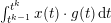 $\int _{t^{k-1}}^{t^{k}}x(t)\cdot g(t)\,\text{d}t$
can be approximated more generally via the Taylor series
 $$\begin{eqnarray}\int _{t^{k-1}}^{t^{k}}x(t)\cdot g(t)\,\text{d}t\approx \mathop{\sum }_{r=0}^{\infty }\displaystyle \frac{x^{(r)}(t^{k-1})}{r!}\cdot \int _{t^{k-1}}^{t^{k}}g(t)t^{r}\,\text{d}t,\end{eqnarray}$$
and with clever programming of
 $g$
, other moments such as velocity or acceleration can be so encoded. In the following, we assume that the radio-frequency pulse sequence and the gradient coils are programmed such that we first encode the velocity in the
 $z$
-direction, that is, for
 $x=(x_{1},x_{2},x_{3})$
and
 $g(t)=(g_{1}(t),g_{2}(t),g_{3}(t))$
we have
 $$\begin{eqnarray}\int _{0}^{t_{0}}x(t)\cdot g(t)\,\text{d}t\approx \underbrace{x_{3}^{\prime }(0)}_{=:v_{z}}\int _{0}^{t_{0}}g_{3}(t)\,t\,\text{d}t,\end{eqnarray}$$
in the interval
 $[0,t_{0}]$
, and then perform the spatial encoding such that
 $$\begin{eqnarray}\int _{t_{k-1}}^{t^{k}}x(t)\cdot g(t)\,\text{d}t\approx \left(\begin{array}{@{}c@{}}x_{1}(t_{k-1})\\ x_{2}(t_{k-1})\end{array}\right)\cdot \int _{t^{k-1}}^{t^{k}}\left(\begin{array}{@{}c@{}}g_{1}(t)\\ g_{2}(t)\end{array}\right)\,\text{d}t\end{eqnarray}$$
holds true for
 $t_{0}<t_{1}<\cdots <t_{m}=T$
. Then, with
 $x=(x_{1}(t_{k-1}),x_{2}(t_{k-1}))$
and
 $g=(g_{1},g_{2})$
as an abuse of notation,
 ${\mathcal{F}}$
reads as
 $$\begin{eqnarray}\displaystyle ({\mathcal{F}}(u,v_{z}))(t^{k})=\displaystyle \frac{1}{2\unicode[STIX]{x1D70B}}\int _{\mathbb{R}^{2}}u(x)\exp (-\text{i}\unicode[STIX]{x1D70E}v_{z}(x))\exp \biggl(-\text{i}x\cdot \int _{t^{k-1}}^{t^{k}}g(t)\,\text{d}t\biggr)\,\text{d}x, & & \displaystyle\end{eqnarray}$$
for some constant
 $\unicode[STIX]{x1D70E}$
. In order to avoid non-linearity of the forward model, we couple
 $u$
and
 $v_{z}$
by simply defining
 $w:=u\exp (-\text{i}\unicode[STIX]{x1D70E}v_{z})$
. Then the forward model
 ${\mathcal{F}}$
simply reduces to the (sub-sampled) Fourier transform.
Benning et al. (Reference Benning, Gladden, Holland, Schönlieb and Valkonen2014) have investigated three choices for regularization functionals: assuming
 $\unicode[STIX]{x1D736}=(\unicode[STIX]{x1D6FC},\unicode[STIX]{x1D6FD})$
, we have
 $$\begin{eqnarray}\displaystyle J(w,\unicode[STIX]{x1D6FC},\unicode[STIX]{x1D6FD})=\unicode[STIX]{x1D6FC}\left\{\begin{array}{@{}l@{}}\text{TV}(w),\quad \\ \text{TGV}_{\unicode[STIX]{x1D6FD}}^{2}(w),\quad \\ \mathop{\sum }_{j=1}^{\infty }|\langle w,\unicode[STIX]{x1D711}_{j}\rangle |.\quad \end{array}\right. & & \displaystyle\end{eqnarray}$$
Here
 $\{\unicode[STIX]{x1D711}_{j}\}_{j\in \mathbb{Z}}$
denotes a wavelet basis, and
 $\text{TGV}_{\unicode[STIX]{x1D6FD}}^{2}$
is the second-order total generalized variation in the sense of Bredies and Valkonen (Reference Bredies and Valkonen2011, Theorem 3.1). In Figure 8.2 we see computational solutions of (8.1) for the choice
 $J(w,\unicode[STIX]{x1D6FC},\unicode[STIX]{x1D6FD})=\text{TGV}_{\unicode[STIX]{x1D6FD}}^{2}(w)$
, a spiral sub-sampling strategy on a Cartesian grid (see Figure 8.1), and the parameter choices
 $\unicode[STIX]{x1D6FC}=0.1$
and
 $\unicode[STIX]{x1D6FD}=3$
. These results have again been computed with the PDHGM. Subsequently,
 $v_{z}$
was extracted as the principal value of the reconstruction
 $w\in R(f^{\unicode[STIX]{x1D6FF}},\unicode[STIX]{x1D6FC},\unicode[STIX]{x1D6FD})$
. The reconstructed
 $z$
-velocity
 $v_{z}$
is subsequently unwrapped by solving the linear system
 $$\begin{eqnarray}\unicode[STIX]{x1D6E5}\hat{v}_{z}=\cos (v_{z})\unicode[STIX]{x1D6E5}\sin (v_{z})-\sin (v_{z})\unicode[STIX]{x1D6E5}\cos (v_{z})\end{eqnarray}$$
for
 $\hat{v}_{z}$
. Here
 $\unicode[STIX]{x1D6E5}$
denotes the Laplace operator. The unwrapped reconstructed velocity
 $\hat{v}_{z}$
is visualized in Figure 8.3.
In order to demonstrate the capabilities of the Bregman iteration, Benning et al. (Reference Benning, Gladden, Holland, Schönlieb and Valkonen2014) have qualitatively analysed Algorithm 1 for different sub-sampling strategies and different initial choices of
 $\unicode[STIX]{x1D6FC}>0$
. These comparisons for different sub-sampling strategies are visualized in Figure 8.4. In Figure 8.5 we see the magnitude images of 20 Bregman iterations computed with Algorithm 1 for the same set-up as described earlier, and the parameter choices
 $\unicode[STIX]{x1D6FC}=1.5$
and
 $\unicode[STIX]{x1D6FD}=3$
.
The structural similarity index measure (SSIM) (see Wang, Bovik, Sheikh and Simoncelli Reference Wang, Bovik, Sheikh and Simoncelli2004) of the magnitude images (a–f) and the velocity images (g–l) for Bregmanized TV reconstructions of computer-generated test data with various sampling patterns and noise
 $\unicode[STIX]{x1D70E}=0.2$
. The parameter
 $\unicode[STIX]{x1D6FC}$
is on the horizontal axis and the Bregman iteration is on the vertical axis. The colours code the SSIM value, also shown in the small lower graph. The continuous line corresponds to violation of the discrepancy principle, and the dashed line to the optimal SSIM. The dash-dotted line in the small graph indicates the SSIM for the first iteration. From Benning et al. (Reference Benning, Gladden, Holland, Schönlieb and Valkonen2014).

Magnitude images of 20 Bregman iterations computed via Algorithm 1, with
 $\unicode[STIX]{x1D6FC}=1.5$
and
 $\unicode[STIX]{x1D6FD}=3$
.

We refer to Benning et al. (Reference Benning, Gladden, Holland, Schönlieb and Valkonen2014) for more information on iterative regularization in the context of velocity-encoded MRI.
8.2 Dynamic MRI with structural prior
Dynamic MRI is a topic of high current relevance in biomedical imaging, with different techniques such as fMRI or DCE-MRI. The basic issue is to reconstruct a sequence of images
 $u=(u_{1},\ldots ,u_{T})$
from measurements
 $(K_{1}u_{1},\ldots ,K_{T}u_{T})$
, with
 $K_{t}$
being a sub-sampled Fourier transform (with different sub-sampling at each time step). Due to the significant measurement times in MRI the sub-sampling is necessary to obtain a significant time resolution; the time resolution will improve with stronger undersampling (e.g. in spokes). The natural data fidelity in this case is thus
 $$\begin{eqnarray}F(Ku,f)=\displaystyle \frac{1}{2}\mathop{\sum }_{t=1}^{T}\Vert K_{t}u_{t}-f_{t}\Vert ^{2}.\end{eqnarray}$$
With substantial undersampling it is hopeless to reconstruct meaningful images from the data at a single time step, hence a regularization in time is needed in order to exploit correlations between close time steps. A natural assumption is smoothness in the time direction, for then a discrete gradient
 $\Vert u_{t+1}-u_{t}\Vert ^{2}$
can be penalized in a regularization functional. Moreover, in order to take into account the edges it is natural to include some total variation regularization for each
 $u_{t}$
. So far, this is an approach that can be used for many dynamic reconstruction problems. A particular feature of such MR investigations, however, is the existence of a structural prior
 $u_{0}$
, which is a high-resolution MR image at different contrast (e.g. a standard anatomical T1 scan) taken before the start of the dynamic imaging. The prior is reconstructed from a very dense sampling and thus at very high resolution. The important step is to notice that most edges in the images
 $u_{t}$
will arise from anatomical structures, and are thus present in
 $u_{0}$
. Hence, an additional structural regularization like the infimal convolution of Bregman distances
 $$\begin{eqnarray}ICBV^{p_{0}}(\cdot ,u_{0})=D_{TV}^{p_{0}}(\cdot ,u_{0})\Box D_{TV}^{-p_{0}}(\cdot ,-u_{0})\end{eqnarray}$$
can be used to achieve super-resolution in the dynamic imaging series.
The regularization functional
 $$\begin{eqnarray}J(u)=\mathop{\sum }_{t=1}^{T}\unicode[STIX]{x1D714}_{t}|u_{t}|_{BV}+\mathop{\sum }_{t=1}^{T}(1-\unicode[STIX]{x1D714}_{t})ICBV^{p_{0}}(u,u_{0})+\mathop{\sum }_{t=1}^{T-1}\displaystyle \frac{\unicode[STIX]{x1D6FE}_{t}}{2}\Vert u_{t+1}-u_{t}\Vert ^{2}\end{eqnarray}$$
combining the three parts was proposed and investigated in Rasch et al. (Reference Rasch, Kolehmainen, Nivajärvi, Kettunen, Gröhn, Burger and Brinkmann2017). The results indicate enormous potential for obtaining reconstructions at high resolution from rather extreme undersamplings in time. These are illustrated in Figure 8.6 for several different time steps of a simulated data set. The first line shows the sampling at different time steps; the last column shows the prior image
 $u_{0}$
instead. The second line provides direct reconstruction without regularization (note that the Fourier transform is continuously invertible, so without undersampling the direct inversion is a standard technique). The third line displays the results with the proposed method, to be compared to the ground truth used for simulating data in the fourth line. These results were obtained on simulated MR data; we refer to Rasch et al. (Reference Rasch, Kolehmainen, Nivajärvi, Kettunen, Gröhn, Burger and Brinkmann2017) for a further study of real data.
Results of undersampled dynamic MRI reconstruction with different methods at five different time steps.

8.3 Nonlinear spectral image fusion
Illustration of the pipeline for facial image fusion using nonlinear spectral decompositions. From Benning et al. (Reference Benning, Möller, Nossek, Burger, Cremers, Gilboa, Schönlieb and Lauze2017d ).

The nonlinear spectral transform as introduced in Section 7.3 can be used to suppress, enhance or extract features of signals at different scales. Benning et al. (Reference Benning, Möller, Nossek, Burger, Cremers, Gilboa, Schönlieb and Lauze2017d
) have used it to fuse features at different scales from two images into a single image, in order to create realistic-looking image fusions. The mathematical procedure is as follows. Given two images, both images are preprocessed such that they are aligned (registered) and that regions within the images are segmented such that the images are fused only in selected regions. Denoting the registered images as
 $f_{1}$
and
 $f_{2}$
, they can be represented via their spectral transforms, that is,
 $$\begin{eqnarray}u_{1}={\mathcal{S}}(f_{1},(u)_{n=0}^{k^{\ast }},\mathbf{c}_{1},\unicode[STIX]{x1D6FC})+\underbrace{f_{1}-{\mathcal{S}}(f_{1},(u)_{n=0}^{k^{\ast }},\text{}\text{1},\unicode[STIX]{x1D6FC})}_{=:r_{1}^{\unicode[STIX]{x1D6FC},k^{\ast }}},\end{eqnarray}$$
and
 $$\begin{eqnarray}u_{2}={\mathcal{S}}(f_{2},(u)_{n=0}^{k^{\ast }},\mathbf{c}_{2},\unicode[STIX]{x1D6FC})+\underbrace{f_{2}-{\mathcal{S}}(f_{2},(u)_{n=0}^{k^{\ast }},\text{}\text{1},\unicode[STIX]{x1D6FC})}_{=:r_{2}^{\unicode[STIX]{x1D6FC},k^{\ast }}},\end{eqnarray}$$
for
 $k^{\ast }\geq 1$
,
 $\unicode[STIX]{x1D6FC}\in A$
and coefficients
 $\mathbf{c}_{1}\in \mathbb{R}^{k^{\ast }}$
,
 $\mathbf{c}_{2}\in \mathbb{R}^{k^{\ast }}$
and
 $\text{}\text{1}\in \{1\}^{k^{\ast }}$
being the constant one-vector. Obviously we have
 $u_{1}=f_{1}$
and
 $u_{2}=f_{2}$
if
 $\mathbf{c}_{1}=\text{}\text{1}$
and
 $\mathbf{c}_{2}=\text{}\text{1}$
.
In order to incorporate the face segmentation into the image fusion process, we allow the coefficient vectors
 $\mathbf{c}_{1}$
and
 $\mathbf{c}_{2}$
to be spatially varying functions
 $\mathbf{c}_{1}:\unicode[STIX]{x1D6FA}\rightarrow \mathbb{R}^{k^{\ast }}$
and
 $\mathbf{c}_{2}:\unicode[STIX]{x1D6FA}\rightarrow \mathbb{R}^{k^{\ast }}$
, respectively. Here
 $\unicode[STIX]{x1D6FA}$
denotes the image domain. The image fusion process can then be mathematically described by
 $$\begin{eqnarray}u_{\text{fused}}:={\mathcal{S}}(f_{1},k^{\ast },\unicode[STIX]{x1D6FC},\mathbf{c}_{1})+{\mathcal{S}}(f_{2},k^{\ast },\unicode[STIX]{x1D6FC},\mathbf{c}_{2})+r_{1}^{\unicode[STIX]{x1D6FC},k^{\ast }}.\end{eqnarray}$$
The individual steps of the image fusion pipeline are visualized in Figure 8.7. For challenging examples this automation may very well fail. Nevertheless, the spectral image fusion still works if registration and segmentation are carried out manually, as can be seen in Figure 8.8. For more information on the nonlinear spectral image fusion we refer to Benning et al. (Reference Benning, Möller, Nossek, Burger, Cremers, Gilboa, Schönlieb and Lauze2017d ).
Image fusion using the nonlinear spectral TV decomposition for the challenging example of fusing a banknote with a picture of Gauss and a painting of Newton. From the supplementary material of Benning et al. (Reference Benning, Möller, Nossek, Burger, Cremers, Gilboa, Schönlieb and Lauze2017d ).

9 Advanced issues
In the following we comment on some advanced issues related to iterative variational methods extending those presented above, namely extensions to non-convex problems, in particular with respect to data fidelities in nonlinear inverse problems, and to modern machine learning approaches.
9.1 Non-convex optimization
In the context of inverse problems one usually deals with data fidelities of the form
 $F(Ku,f^{\unicode[STIX]{x1D6FF}})$
that measure the deviation between
 $Ku$
and
 $f^{\unicode[STIX]{x1D6FF}}$
in some sense. So far we have always assumed this particular structure, and also that
 $F$
is convex. Both assumptions can be relaxed. In the following we assume that we simply have some non-convex energy functional
 $E:{\mathcal{U}}\rightarrow \mathbb{R}$
that is Fréchet-differentiable with gradient
 $\unicode[STIX]{x1D6FB}E$
. As there might not exist critical points, or finding them might be unstable due to ill-posedness, it makes sense to generalize (5.3) to
 $$\begin{eqnarray}\displaystyle R(\unicode[STIX]{x1D736})=\underset{u\in {\mathcal{U}}}{\operatorname{argmin}}\,\{E(u)+J(u,\unicode[STIX]{x1D736})\}. & & \displaystyle\end{eqnarray}$$
Here we want to emphasize that
 $R(\unicode[STIX]{x1D736})$
is not necessarily a regularization operator in the classical sense, as in general we do not make the dependence on some data
 $f^{\unicode[STIX]{x1D6FF}}$
explicit. In Section 9.2 we particularly investigate the case in which
 $E$
is of the form
 $E(\cdot )=F(K(\cdot ),f^{\unicode[STIX]{x1D6FF}})$
, where
 $K$
stems from a nonlinear inverse problem, and where
 $F(\cdot ,f^{\unicode[STIX]{x1D6FF}})$
is potentially non-convex in its first argument.
It is important to emphasize that even for non-smooth, non-convex optimization, there is a vast number of recent publications: forward–backward or proximal-type schemes (Attouch and Bolte Reference Attouch and Bolte2009, Attouch, Bolte, Redont and Soubeyran Reference Attouch, Bolte, Redont and Soubeyran2010, Attouch, Bolte and Svaiter Reference Attouch, Bolte and Svaiter2013, Bonettini, Loris, Porta and Prato Reference Bonettini, Loris, Porta and Prato2016, Bonettini et al.
Reference Bonettini, Loris, Porta, Prato and Rebegoldi2017), linearized proximal schemes (Xu and Yin Reference Xu and Yin2013, Bolte, Sabach and Teboulle Reference Bolte, Sabach and Teboulle2014, Xu and Yin Reference Xu and Yin2017, Nikolova and Tan Reference Nikolova and Tan2017), inertial methods (Ochs, Chen, Brox and Pock Reference Ochs, Chen, Brox and Pock2014, Pock and Sabach Reference Pock and Sabach2016), primal–dual algorithms (Valkonen Reference Valkonen2014, Li and Pong Reference Li and Pong2015, Moeller, Benning, Schönlieb and Cremers Reference Moeller, Benning, Schönlieb and Cremers2015, Benning, Knoll, Schönlieb and Valkonen Reference Benning, Knoll, Schönlieb, Valkonen and Bociu2015), scaled gradient projection methods (Prato et al.
Reference Prato, Bonettini, Loris, Porta and Rebegoldi2016), non-smooth Gauss–Newton extensions (Drusvyatskiy, Ioffe and Lewis Reference Drusvyatskiy, Ioffe and Lewis2016, Ochs, Fadili and Brox Reference Ochs, Fadili and Brox2017), and nonlinear eigenproblems (Hein and Bühler Reference Hein, Bühler and Lafferty2010, Bresson, Laurent, Uminsky and Brecht Reference Bresson, Laurent, Uminsky, Brecht and Pereira2012, Benning, Gilboa and Schönlieb Reference Benning, Gilboa and Schönlieb2016, Boţ and Csetnek Reference Boţ and Csetnek2017, Laurent, von Brecht, Bresson and Szlam Reference Laurent, von Brecht, Bresson, Szlam and Lee2016, Benning, Gilboa, Grah and Schönlieb Reference Benning, Gilboa, Grah, Schönlieb and Lauze2017c
). Here we focus mainly on recent generalizations of the proximal gradient method and the linearized Bregman iteration for non-convex functionals
 $E$
; a treatment of all the algorithms mentioned above would be a subject for a survey paper in its own right.
9.1.1 Proximal gradient method
The most basic approach to finding solutions of (9.1) iteratively is via proximal gradient descent, that is, forward–backward splitting (Lions and Mercier Reference Lions and Mercier1979). The idea is to linearize the non-convex part
 $E$
and to add a damping with respect to the previous iterate. If we allow this damping to be carried out via a Bregman distance with respect to a Legendre functional
 $H$
, we obtain the recently proposed Bregman proximal gradient method (Bolte, Sabach, Teboulle and Vaisbourd Reference Bolte, Sabach, Teboulle and Vaisbourd2017):
 $$\begin{eqnarray}\displaystyle R(u^{k-1},\unicode[STIX]{x1D736}) & = & \displaystyle \underset{u\in {\mathcal{U}}}{\operatorname{argmin}}\,\{\unicode[STIX]{x1D6FC}^{k-1}\langle \unicode[STIX]{x1D6FB}E(u^{k-1}),u-u^{k-1}\rangle \nonumber\\ \displaystyle & & \displaystyle \quad +\,D_{H}^{}(u,u^{k-1})+\unicode[STIX]{x1D6FC}^{k-1}J(u,\unicode[STIX]{x1D736})\},\nonumber\\ \displaystyle u^{k} & \in & \displaystyle R(u^{k-1},\unicode[STIX]{x1D736}),\end{eqnarray}$$
for
 $\unicode[STIX]{x1D736}=(\unicode[STIX]{x1D6FC},\unicode[STIX]{x1D6FC}^{0},\ldots ,\unicode[STIX]{x1D6FC}^{k-1})$
. Here we want to emphasize that
 $R(u^{k-1},\unicode[STIX]{x1D736})$
is no longer a regularization operator in the classical sense as we are no longer necessarily dealing with an inverse problem. Obviously, if
 $E$
is a (potentially non-convex) data fidelity functional of some nonlinear inverse problem,
 $R(u^{k-1},p^{k-1},\unicode[STIX]{x1D736})$
depends on some data
 $f^{\unicode[STIX]{x1D6FF}}$
and we again deal with a regularization problem, which this time approaches the solution of a (potentially) nonlinear inverse problem. This more specific scenario will be addressed in Section 9.2. Without additional assumptions on
 $E$
,
 $H$
and
 $J$
there is little chance that we can carry out a convergence analysis for (9.2) or even prove existence of the updates. A typical assumption is Lipschitz-continuity of
 $\unicode[STIX]{x1D6FB}E$
, that is, we guarantee
 $$\begin{eqnarray}\Vert \unicode[STIX]{x1D6FB}E(u)-\unicode[STIX]{x1D6FB}E(v)\Vert _{{\mathcal{U}}^{\ast }}\leq L\Vert u-v\Vert _{{\mathcal{U}}}\end{eqnarray}$$
for all
 $u,v\in {\mathcal{U}}$
and a constant
 $L>0$
. A nice aspect of this property is that it implies convexity of the family of functionals
 $$\begin{eqnarray}\displaystyle \displaystyle \frac{L}{\unicode[STIX]{x1D6FE}_{i}}H_{i}-E & & \displaystyle\end{eqnarray}$$
(see Bauschke, Bolte and Teboulle Reference Bauschke, Bolte and Teboulle2016, Benning, Betcke, Ehrhardt and Schönlieb Reference Benning, Betcke, Ehrhardt, Schönlieb and Quispel2017b
, Bolte et al. Reference Bolte, Sabach, Teboulle and Vaisbourd2017), where
 $\{H_{i}\}_{i=1,\ldots }$
is a family of
 $\unicode[STIX]{x1D6FE}_{i}$
-strongly convex functionals, that is,
 $$\begin{eqnarray}\displaystyle \frac{\unicode[STIX]{x1D6FE}_{i}}{2}\Vert u-v\Vert _{{\mathcal{U}}}^{2}\leq D_{H_{i}}^{}(u,v),\end{eqnarray}$$
for all
 $u,v\in {\mathcal{U}}$
. Let us now assume that
 $H$
in (9.2) is a member of (9.3) with strong convexity constant
 $\unicode[STIX]{x1D6FE}$
, that is,
 $$\begin{eqnarray}\displaystyle H_{\unicode[STIX]{x1D6FE}}(u):=\displaystyle \frac{L}{\unicode[STIX]{x1D6FE}}H(u)-E(u) & & \displaystyle\end{eqnarray}$$
is convex for all
 $u\in {\mathcal{U}}$
. Then this convexity assumption is already enough to ensure a sufficient decrease of the energy
 $E+J$
in each iteration of (9.2).
Lemma 9.1. Suppose
 $E$
is coercive or has bounded level sets,
 $\inf _{u}E(u)>-\infty$
and
 $\unicode[STIX]{x1D6FB}E$
is Lipschitz continuous with constant
 $L$
, and let
 $H$
be a Legendre functional in the sense of Definition 5.11, which is also
 $\unicode[STIX]{x1D6FE}$
-strongly convex. Further assume
 $$\begin{eqnarray}\displaystyle 0<\unicode[STIX]{x1D6FC}^{k-1}<\displaystyle \frac{\unicode[STIX]{x1D6FE}C^{k}}{L+\unicode[STIX]{x1D6FE}C^{k}\unicode[STIX]{x1D70C}}\quad \text{for }~C^{k}:=\displaystyle \frac{D_{H}^{\text{symm}}(u^{k},u^{k-1})}{D_{H}^{}(u^{k},u^{k-1})}, & & \displaystyle\end{eqnarray}$$
for a constant
 $\unicode[STIX]{x1D70C}>0$
, for all
 $k\in \mathbb{N}$
, and that
 $E+J(\cdot ,\unicode[STIX]{x1D6FC})$
has at least one critical point. Then the iterates of (9.2) satisfy
 $$\begin{eqnarray}\displaystyle E(u^{k})+J(u^{k},\unicode[STIX]{x1D6FC})+\unicode[STIX]{x1D70C}D_{H}^{\text{symm}}(u^{k},u^{k-1})\leq E(u^{k-1})+J(u^{k-1},\unicode[STIX]{x1D6FC}), & & \displaystyle\end{eqnarray}$$
for
 $u^{k}\in R(u^{k-1},\unicode[STIX]{x1D736})$
and all
 $k\in \mathbb{N}$
.
Proof. From the convexity of (9.4) we immediately observe
 $$\begin{eqnarray}\displaystyle 0\leq D_{H_{\unicode[STIX]{x1D6FE}}}^{}(u^{k},u^{k-1}) & = & \displaystyle \displaystyle \frac{L}{\unicode[STIX]{x1D6FE}}D_{H}^{}(u^{k},u^{k-1})\nonumber\\ \displaystyle & & \displaystyle \quad -\,(E(u^{k})-E(u^{k-1})-\langle \unicode[STIX]{x1D6FB}E(u^{k-1}),u^{k}-u^{k-1}\rangle ).\nonumber\end{eqnarray}$$
As a direct consequence, we have derived the estimate
 $$\begin{eqnarray}\displaystyle E(u^{k})+\langle \unicode[STIX]{x1D6FB}E(u^{k-1}),u^{k-1}-u^{k}\rangle -\displaystyle \frac{L}{\unicode[STIX]{x1D6FE}}D_{H}^{}(u^{k},u^{k-1})\leq E(u^{k-1}). & & \displaystyle\end{eqnarray}$$
From the optimality condition of (9.2) we obtain
 $$\begin{eqnarray}\displaystyle \unicode[STIX]{x1D6FB}E(u^{k-1})=\displaystyle \frac{1}{\unicode[STIX]{x1D6FC}^{k-1}}(\unicode[STIX]{x1D6FB}H(u^{k-1})-\unicode[STIX]{x1D6FB}H(u^{k}))-p^{k}, & & \displaystyle\end{eqnarray}$$
for
 $p^{k}\in \unicode[STIX]{x2202}J(u^{k},\unicode[STIX]{x1D6FC})$
. Inserting (9.8) into (9.7) yields
 $$\begin{eqnarray}\displaystyle & & \displaystyle E(u^{k})+\displaystyle \frac{1}{\unicode[STIX]{x1D6FC}^{k-1}}D_{H}^{\text{symm}}(u^{k},u^{k-1})-\displaystyle \frac{L}{\unicode[STIX]{x1D6FE}}D_{H}^{}(u^{k},u^{k-1})\nonumber\\ \displaystyle & & \displaystyle \quad \leq E(u^{k-1})+\langle p^{k},u^{k-1}-u^{k}\rangle .\end{eqnarray}$$
Due to the convexity of
 $J(\cdot ,\unicode[STIX]{x1D6FC})$
we can estimate
 $$\begin{eqnarray}\langle p^{k},u^{k-1}-u^{k}\rangle \leq J(u^{k-1},\unicode[STIX]{x1D6FC})-J(u^{k},\unicode[STIX]{x1D6FC}).\end{eqnarray}$$
Applying this estimate to (9.9) results in
 $$\begin{eqnarray}\displaystyle & & \displaystyle E(u^{k})+J(u^{k},\unicode[STIX]{x1D6FC})+\displaystyle \frac{1}{\unicode[STIX]{x1D6FC}^{k-1}}D_{H}^{\text{symm}}(u^{k},u^{k-1})-\displaystyle \frac{L}{\unicode[STIX]{x1D6FE}}D_{H}^{}(u^{k},u^{k-1})\nonumber\\ \displaystyle & & \displaystyle \quad \leq E(u^{k-1})+J(u^{k-1},\unicode[STIX]{x1D6FC}).\nonumber\end{eqnarray}$$
Together with the stepsize bound (9.5) this concludes the proof. ☐
Remark 9.2. Note that we have not made use of the Lipschitz continuity of
 $\unicode[STIX]{x1D6FB}E$
, but only of the convexity of (9.4) in order to obtain a sufficient decrease.
Remark 9.3. Due to the
 $\unicode[STIX]{x1D6FE}$
-strong convexity of
 $H$
, the estimate (9.6) automatically implies
 $$\begin{eqnarray}\displaystyle E(u^{k})+J(u^{k},\unicode[STIX]{x1D6FC})+\unicode[STIX]{x1D70C}\unicode[STIX]{x1D6FE}\Vert u^{k}-u^{k-1}\Vert _{{\mathcal{U}}}^{2}\leq E(u^{k-1})+J(u^{k-1},\unicode[STIX]{x1D6FC}). & & \displaystyle\end{eqnarray}$$
If we additionally assume that both
 $\unicode[STIX]{x1D6FB}E$
and
 $\unicode[STIX]{x1D6FB}H$
are Lipschitz-continuous, we further obtain a bound for the gradient of the energy
 $E+J$
at iterate
 $u^{k}$
.
Lemma 9.4. Suppose the same assumptions hold as in Lemma 9.1. We further assume that
 $\unicode[STIX]{x1D6FB}E$
is Lipschitz-continuous with constant
 $L$
and
 $\unicode[STIX]{x1D6FB}H$
is Lipschitz-continuous with constant
 $\unicode[STIX]{x1D6FF}$
. Then we observe
 $$\begin{eqnarray}\Vert \unicode[STIX]{x1D6FB}E(u^{k})+p^{k}\Vert _{{\mathcal{U}}^{\ast }}\leq \biggl(L+\displaystyle \frac{\unicode[STIX]{x1D6FF}}{\unicode[STIX]{x1D6FC}^{k-1}}\biggr)\Vert u^{k}-u^{k-1}\Vert _{{\mathcal{U}}}\end{eqnarray}$$
for all
 $p^{k}\in \unicode[STIX]{x2202}J(u^{k},\unicode[STIX]{x1D6FC})$
.
Proof. This follows trivially from (9.8) and the Lipschitz-continuity of both
 $\unicode[STIX]{x1D6FB}E$
and
 $\unicode[STIX]{x1D6FB}H$
. ☐
In a finite-dimensional setting
 ${\mathcal{U}}=\mathbb{R}^{n}$
it is now sufficient to assume that
 $E+J$
is a Kurdyka–Łojasiewicz (KL) function (Lojasiewicz Reference Lojasiewicz1963, Kurdyka Reference Kurdyka1998, Bolte, Daniilidis and Lewis Reference Bolte, Daniilidis and Lewis2007) in order to show that the iterates (9.2) converge globally to a critical point of
 $E+J$
.
Theorem 9.5. Let the same assumptions hold true as in Lemma 9.4. Further assume
 ${\mathcal{U}}=\mathbb{R}^{n}$
and that
 $E+J$
is a KL function that has at least one critical point. Then the iterates (9.2) converge globally to a critical point of the energy
 $E+J$
.
Proof. See the proof of Bolte et al. (Reference Bolte, Sabach, Teboulle and Vaisbourd2017, Theorem 4.1(ii)). ☐
We refer the reader to Bolte, Daniilidis, Ley and Mazet (Reference Bolte, Daniilidis, Ley and Mazet2010) for a detailed investigation of the class of KL functions, and to Bolte et al. (Reference Bolte, Sabach, Teboulle and Vaisbourd2017) for more information on the Bregman proximal gradient.
9.1.2 Linearized Bregman iteration for non-convex functionals
The linearized Bregman iteration introduced in Section 6.2 can easily be adapted to tackle general, non-convex optimization problems. Suppose a Fréchet-differentiable functional
 $E:{\mathcal{U}}\rightarrow \mathbb{R}$
with Fréchet-gradient
 $\unicode[STIX]{x1D6FB}E$
; then we can simply modify Algorithm 2 to
 $$\begin{eqnarray}\displaystyle R(u^{k-1},p^{k-1},\unicode[STIX]{x1D736}) & = & \displaystyle \underset{u\in {\mathcal{U}}}{\operatorname{argmin}}\,\{\langle \unicode[STIX]{x1D6FB}E(u^{k-1}),u-u^{k-1}\rangle +\unicode[STIX]{x1D6FC}^{k-1}D_{J(\cdot ,\unicode[STIX]{x1D6FC})}^{p^{k-1}}(u,u^{k-1})\}\nonumber\\ \displaystyle u^{k} & \in & \displaystyle R(u^{k-1},p^{k-1},\unicode[STIX]{x1D736})\nonumber\\ \displaystyle p^{k} & = & \displaystyle p^{k-1}-\displaystyle \frac{1}{\unicode[STIX]{x1D6FC}^{k-1}}\unicode[STIX]{x1D6FB}E(u^{k-1}),\end{eqnarray}$$
for
 $\unicode[STIX]{x1D736}=(\unicode[STIX]{x1D6FC},\unicode[STIX]{x1D6FC}^{0},\ldots ,\unicode[STIX]{x1D6FC}^{k-1})$
and
 $p^{k-1}\in \unicode[STIX]{x2202}J(u^{k-1},\unicode[STIX]{x1D6FC})$
. This method for arbitrary non-convex energies
 $E$
was introduced in Benning, Betcke, Ehrhardt and Schönlieb (Reference Benning, Betcke, Ehrhardt, Schönlieb and Quispel2017b
) and mathematically analysed in Benning, Betcke, Ehrhardt and Schönlieb (Reference Benning, Betcke, Ehrhardt and Schönlieb2017a
). As in Section 9.1.1,
 $R(u^{k-1},p^{k-1},\unicode[STIX]{x1D736})$
is no longer a regularization operator in the classical sense, unless
 $E$
is a (potentially non-convex) data fidelity function for some nonlinear inverse problem.
It becomes evident that (9.11) and (9.2) coincide if
 $J$
in (9.11) is a Legendre functional and if
 $J$
in (9.2) is zero. Hence, the convergence analysis closely follows the convergence analysis of the proximal gradient method. We assume that
 $J(\cdot ,\unicode[STIX]{x1D6FC})$
is
 $\unicode[STIX]{x1D6FE}$
-strongly convex and that
 $$\begin{eqnarray}\displaystyle J_{\unicode[STIX]{x1D6FE}}(u,\unicode[STIX]{x1D6FC}):=\displaystyle \frac{L}{\unicode[STIX]{x1D6FE}}J(u,\unicode[STIX]{x1D6FC})-E(u) & & \displaystyle\end{eqnarray}$$
is convex. Then we can show the following sufficient decrease of the energy (Benning et al. Reference Benning, Betcke, Ehrhardt, Schönlieb and Quispel2017b ).
Lemma 9.6. Suppose
 $E$
is coercive or has bounded level sets,
 $\inf _{u}E(u)>-\infty$
,
 $\unicode[STIX]{x1D6FC}^{k-1}$
satisfies (9.5) with
 $$\begin{eqnarray}C^{k}:=\displaystyle \frac{D_{J(\cdot ,\unicode[STIX]{x1D6FC})}^{\text{symm}}(u^{k},u^{k-1})}{D_{J(\cdot ,\unicode[STIX]{x1D6FC})}^{p^{k-1}}(u^{k},u^{k-1})},\end{eqnarray}$$
and that
 $E$
has at least one critical point. Then the iterates of (9.11) satisfy
 $$\begin{eqnarray}\displaystyle E(u^{k})+\unicode[STIX]{x1D70C}D_{J(\cdot ,\unicode[STIX]{x1D6FC})}^{p^{k-1}}(u^{k},u^{k-1})\leq E(u^{k-1}). & & \displaystyle\end{eqnarray}$$
Proof. From the convexity of (9.12) we immediately observe
 $$\begin{eqnarray}\displaystyle 0\leq D_{J_{\unicode[STIX]{x1D6FE}}(\cdot ,\unicode[STIX]{x1D6FC})}^{q^{k-1}}(u^{k},u^{k-1}) & = & \displaystyle \displaystyle \frac{L}{\unicode[STIX]{x1D6FE}}D_{J(\cdot ,\unicode[STIX]{x1D6FC})}^{p^{k-1}}(u^{k},u^{k-1})\nonumber\\ \displaystyle & & \displaystyle \quad -\,(E(u^{k})-E(u^{k-1})-\langle \unicode[STIX]{x1D6FB}E(u^{k-1}),u^{k}-u^{k-1}\rangle ),\nonumber\end{eqnarray}$$
for
 $q^{k-1}\in \unicode[STIX]{x2202}J_{\unicode[STIX]{x1D6FE}}(u,\unicode[STIX]{x1D6FC})$
. As a direct consequence, we have derived the estimate
 $$\begin{eqnarray}\displaystyle E(u^{k})+\langle \unicode[STIX]{x1D6FB}E(u^{k-1}),u^{k-1}-u^{k}\rangle -\displaystyle \frac{L}{\unicode[STIX]{x1D6FE}}D_{J(\cdot ,\unicode[STIX]{x1D6FC})}^{p^{k-1}}(u^{k},u^{k-1})\leq E(u^{k-1}). & & \displaystyle\end{eqnarray}$$
Inserting the dual update formula of (9.11) into (9.14) then yields
 $$\begin{eqnarray}E(u^{k})+\displaystyle \frac{1}{\unicode[STIX]{x1D6FC}^{k-1}}D_{J(\cdot ,\unicode[STIX]{x1D6FC})}^{\text{symm}}(u^{k},u^{k-1})-\displaystyle \frac{L}{\unicode[STIX]{x1D6FE}}D_{J(\cdot ,\unicode[STIX]{x1D6FC})}^{p^{k-1}}(u^{k},u^{k-1})\leq E(u^{k-1}).\end{eqnarray}$$
Together with the stepsize bound (9.5) we conclude (9.13). ☐
If we further assume that
 $J^{\ast }$
is
 $\unicode[STIX]{x1D6FF}$
-strongly convex with respect to its first argument, that is,
 $$\begin{eqnarray}\displaystyle \frac{\unicode[STIX]{x1D6FF}}{2}\Vert p-q\Vert _{{\mathcal{U}}^{\ast }}^{2}\leq D_{J^{\ast }(\cdot ,\unicode[STIX]{x1D6FC})}^{v}(p,q),\end{eqnarray}$$
for all
 $p,q\in {\mathcal{U}}^{\ast }$
and
 $v\in \unicode[STIX]{x2202}J^{\ast }(q,\unicode[STIX]{x1D6FC})$
, and
 $J^{\ast }$
denoting the convex conjugate of
 $J$
with respect to the first variable, then we can easily derive the following bound for the gradient at each iteration (Benning et al.
Reference Benning, Betcke, Ehrhardt, Schönlieb and Quispel2017b
).
Lemma 9.7. Let the same assumptions hold true as in Lemma 9.6, and further assume that
 $J$
is
 $\unicode[STIX]{x1D6FF}$
-strongly convex for all arguments and corresponding subgradients. Then the iterates (9.11) satisfy
 $$\begin{eqnarray}\Vert \unicode[STIX]{x1D6FB}E(u^{k-1})\Vert _{{\mathcal{U}}^{\ast }}\leq \displaystyle \frac{\unicode[STIX]{x1D6FC}^{k-1}}{\unicode[STIX]{x1D6FF}}\Vert u^{k}-u^{k-1}\Vert _{{\mathcal{U}}},\end{eqnarray}$$
for all
 $k\in \mathbb{N}$
.
Proof. From the standard duality estimate
 $\langle p,u\rangle \leq \Vert u\Vert _{{\mathcal{U}}}\Vert p\Vert _{{\mathcal{U}}^{\ast }}$
, we observe
 $$\begin{eqnarray}D_{J(\cdot ,\unicode[STIX]{x1D6FC})}^{\text{symm}}(p^{k},p^{k-1})=\langle p^{k}-p^{k-1},u^{k}-u^{k-1}\rangle \leq \Vert p^{k}-p^{k-1}\Vert _{{\mathcal{U}}^{\ast }}\Vert u^{k}-u^{k-1}\Vert _{{\mathcal{U}}}.\end{eqnarray}$$
Together with the strong convexity of
 $J^{\ast }(\cdot ,\unicode[STIX]{x1D6FC})$
, we therefore estimate
 $$\begin{eqnarray}\unicode[STIX]{x1D6FF}\Vert p^{k}-p^{k-1}\Vert _{{\mathcal{U}}^{\ast }}\leq \displaystyle \frac{D_{J(\cdot ,\unicode[STIX]{x1D6FC})}^{\text{symm}}(p^{k},p^{k-1})}{\Vert p^{k}-p^{k-1}\Vert _{{\mathcal{U}}^{\ast }}}\leq \Vert u^{k}-u^{k-1}\Vert _{{\mathcal{U}}}.\end{eqnarray}$$
Inserting the dual update formula from (9.11) thus yields
 $$\begin{eqnarray}\displaystyle \frac{\unicode[STIX]{x1D6FF}}{\unicode[STIX]{x1D6FC}^{k-1}}\Vert \unicode[STIX]{x1D6FB}E(u^{k-1})\Vert _{{\mathcal{U}}^{\ast }}\leq \Vert u^{k}-u^{k-1}\Vert _{{\mathcal{U}}}.\end{eqnarray}$$
This concludes the proof. ☐
Note that we require no Lipschitz-continuity assumptions for
 $\unicode[STIX]{x1D6FB}E$
in order for Lemmas 9.6 and 9.7 to apply, but only that (9.12) is convex. As in the case of the proximal gradient method, we can prove global convergence of the iterates (9.11) for finite-dimensional
 ${\mathcal{U}}=\mathbb{R}^{n}$
.
Theorem 9.8. Let the same assumptions hold true as in Lemma 9.6. Further assume
 ${\mathcal{U}}=\mathbb{R}^{n}$
and that
 $E$
is a KL function. Then the iterates (9.11) converge globally to a critical point of the energy
 $E$
.
Proof. The proof is a special case of the more general proof of Benning et al. (Reference Benning, Betcke, Ehrhardt and Schönlieb2017a , Theorem 5.6 & Corollary 5.7). ☐
We do want to emphasize that we require
 $J^{\ast }(\cdot ,\unicode[STIX]{x1D6FC})$
to be strongly convex, which in return implies the restrictive assumption that
 $J(\cdot ,\unicode[STIX]{x1D6FC})$
is a smooth functional with Lipschitz-continuous gradient. In order to get rid of this restrictive condition we split the functional
 $J(\cdot ,\unicode[STIX]{x1D6FC})$
into the two parts
 $$\begin{eqnarray}J(u,\unicode[STIX]{x1D6FC})=H(u)+\displaystyle \frac{1}{\unicode[STIX]{x1D6FC}^{k-1}}G(u,\unicode[STIX]{x1D6FC}),\end{eqnarray}$$
and assume that
 $H$
is
 $\unicode[STIX]{x1D6FE}$
-strongly convex and has
 $\unicode[STIX]{x1D6FF}$
-Lipschitz gradient
 $\unicode[STIX]{x1D6FB}H$
, and that
 $G(\cdot ,\unicode[STIX]{x1D6FC})$
is proper, lower semicontinuous and convex. Hence, we modify (9.11) as follows:
 $$\begin{eqnarray}\displaystyle R(u^{k-1},q^{k-1},\unicode[STIX]{x1D736}) & = & \displaystyle \underset{u\in {\mathcal{U}}}{\operatorname{argmin}}\,\{\langle \unicode[STIX]{x1D6FB}E(u^{k-1}),u-u^{k-1}\rangle \nonumber\\ \displaystyle & & \displaystyle \quad +\,D_{G(\cdot ,\unicode[STIX]{x1D6FC})}^{q^{k-1}}(u,u^{k-1})+\unicode[STIX]{x1D6FC}^{k-1}D_{H}^{}(u,u^{k-1})\},\nonumber\\ \displaystyle u^{k} & \in & \displaystyle R(u^{k-1},q^{k-1},\unicode[STIX]{x1D736}),\nonumber\\ \displaystyle q^{k} & = & \displaystyle q^{k-1}-(\unicode[STIX]{x1D6FB}E(u^{k-1})+\unicode[STIX]{x1D6FC}^{k-1}(\unicode[STIX]{x1D6FB}H(u^{k})-\unicode[STIX]{x1D6FB}H(u^{k-1}))),\end{eqnarray}$$
for
 $q^{0}\in \unicode[STIX]{x2202}G(u^{0},\unicode[STIX]{x1D6FC})$
. We then define the surrogate energy
 $$\begin{eqnarray}\displaystyle E^{k}(u^{k}):=E(u^{k})+D_{G(\cdot ,\unicode[STIX]{x1D6FC})}^{q^{k-1}}(u^{k},u^{k-1}), & & \displaystyle\end{eqnarray}$$
for
 $q^{k-1}\in \unicode[STIX]{x2202}G(u^{k-1},\unicode[STIX]{x1D6FC})$
. For this surrogate energy we can show the following results.
Lemma 9.9. Suppose
 $E$
is coercive or has bounded level sets,
 $\inf _{u}E(u)>-\infty$
and
 $E$
has at least one critical point, and assume
 $H$
is
 $\unicode[STIX]{x1D6FE}$
-strongly convex with
 $\unicode[STIX]{x1D6FF}$
-Lipschitz gradient
 $\unicode[STIX]{x1D6FB}H$
, and
 $\unicode[STIX]{x1D6FC}^{k-1}$
satisfies (9.5). Then the iterates of (9.15) satisfy
 $$\begin{eqnarray}E^{k}(u^{k})+\unicode[STIX]{x1D70C}D_{H}^{}(u^{k},u^{k-1})\leq E^{k-1}(u^{k-1}).\end{eqnarray}$$
Proof. The proof follows the same principle as the proofs of Lemmas 9.1 and 9.6. Convexity of
 ${\textstyle \frac{L}{\unicode[STIX]{x1D6FE}}}H-E$
implies the estimate in (9.7). Inserting the optimality condition (or the dual update formula) of (9.15), applying (9.5) and adding
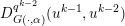 $D_{G(\cdot ,\unicode[STIX]{x1D6FC})}^{q^{k-2}}(u^{k-1},u^{k-2})$
to both sides of the inequality then yields the desired estimate. ☐
A bound of the gradient of
 $E^{k}(u^{k})$
follows from the Lipschitz-continuity of both
 $\unicode[STIX]{x1D6FB}E$
and
 $\unicode[STIX]{x1D6FB}H$
.
Lemma 9.10. Let the same assumptions hold true as in Lemma 9.9. Then the iterates (9.15) satisfy
 $$\begin{eqnarray}\Vert \unicode[STIX]{x1D6FB}E(u^{k})+q^{k}-q^{k-1}\Vert _{{\mathcal{U}}^{\ast }}\leq (L+\unicode[STIX]{x1D6FF}\unicode[STIX]{x1D6FC}^{k-1})\Vert u^{k}-u^{k-1}\Vert _{{\mathcal{U}}}.\end{eqnarray}$$
Proof. Using the dual update formula (9.15) and the Lipschitz-continuity of
 $\unicode[STIX]{x1D6FB}E$
and
 $\unicode[STIX]{x1D6FB}H$
leads to
 $$\begin{eqnarray}\displaystyle & & \displaystyle \Vert \unicode[STIX]{x1D6FB}E(u^{k})+q^{k}-q^{k-1}\Vert _{{\mathcal{U}}^{\ast }}\nonumber\\ \displaystyle & & \displaystyle \quad =\Vert \unicode[STIX]{x1D6FB}E(u^{k})-\unicode[STIX]{x1D6FB}E(u^{k-1})+\unicode[STIX]{x1D6FC}^{k-1}(\unicode[STIX]{x1D6FB}H(u^{k-1})-\unicode[STIX]{x1D6FB}H(u^{k}))\Vert _{{\mathcal{U}}^{\ast }}\nonumber\\ \displaystyle & & \displaystyle \quad \leq L\Vert u^{k}-u^{k-1}\Vert _{{\mathcal{U}}}+\unicode[STIX]{x1D6FC}^{k-1}\unicode[STIX]{x1D6FF}\Vert u^{k-1}-u^{k}\Vert _{{\mathcal{U}}},\nonumber\end{eqnarray}$$
which proves the conjecture. ☐
As in the previous case, global convergence can be achieved under the assumption that the domain is finite-dimensional and that
 $E^{k}(u)$
is a KL-function.
Theorem 9.11. Let the same assumptions hold true as in Lemma 9.10. Further assume
 ${\mathcal{U}}=\mathbb{R}^{n}$
and that
 $E^{k}$
is a KL function for all
 $k\in \mathbb{N}$
. Then the iterates (9.15) converge globally. If, in addition, the sequence
 $\{q^{k}\}_{k\in \mathbb{N}}$
is bounded, then the iterates even convergence to a critical point of the energy
 $E$
.
Proof. The proof is a special case of the more general proof of Benning et al. (Reference Benning, Betcke, Ehrhardt and Schönlieb2017a , Theorem 5.10). ☐
Remark 9.12. Given the structure of the problem, it is also tempting to look at a Fejér-monotonicity with respect to
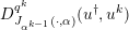 $D_{J_{\unicode[STIX]{x1D6FC}^{k-1}}(\cdot ,\unicode[STIX]{x1D6FC})}^{q^{k}}(u^{\dagger },u^{k})$
, for
 $$\begin{eqnarray}J_{\unicode[STIX]{x1D6FC}^{k-1}}(u,\unicode[STIX]{x1D6FC}):=\unicode[STIX]{x1D6FC}^{k-1}J(u,\unicode[STIX]{x1D6FC})-E(u).\end{eqnarray}$$
If we make the same attempt as in Section 6, we observe
 $$\begin{eqnarray}\displaystyle & & \displaystyle D_{J_{\unicode[STIX]{x1D6FC}^{k-1}}(\cdot ,\unicode[STIX]{x1D6FC})}^{q^{k}}(u^{\dagger },u^{k})-D_{J_{\unicode[STIX]{x1D6FC}^{k-1}}(\cdot ,\unicode[STIX]{x1D6FC})}^{q^{k-1}}(u^{\dagger },u^{k-1})\nonumber\\ \displaystyle & & \displaystyle \quad =-D_{J_{\unicode[STIX]{x1D6FC}^{k-1}}(\cdot ,\unicode[STIX]{x1D6FC})}^{q^{k-1}}(u^{k},u^{k-1})-\langle q^{k}-q^{k-1},u^{\dagger }-u^{k}\rangle ,\nonumber\\ \displaystyle & & \displaystyle \quad =-D_{J_{\unicode[STIX]{x1D6FC}^{k-1}}(\cdot ,\unicode[STIX]{x1D6FC})}^{q^{k-1}}(u^{k},u^{k-1})\nonumber\\ \displaystyle & & \displaystyle \qquad -\,\unicode[STIX]{x1D6FC}^{k-1}\langle p^{k}-p^{k-1},u^{\dagger }-u^{k}\rangle \nonumber\\ \displaystyle & & \displaystyle \qquad +\,\langle \unicode[STIX]{x1D6FB}E(u^{k})-\unicode[STIX]{x1D6FB}E(u^{k-1}),u^{\dagger }-u^{k}\rangle ,\nonumber\\ \displaystyle & & \displaystyle \quad =-D_{J_{\unicode[STIX]{x1D6FC}^{k-1}}(\cdot ,\unicode[STIX]{x1D6FC})}^{q^{k-1}}(u^{k},u^{k-1})\nonumber\\ \displaystyle & & \displaystyle \qquad +\,\langle \unicode[STIX]{x1D6FB}E(u^{k}),u^{\dagger }-u^{k}\rangle \,.\nonumber\end{eqnarray}$$
Since we also know that
 $$\begin{eqnarray}\displaystyle & & \displaystyle \langle \unicode[STIX]{x1D6FB}E(u^{k}),u^{\dagger }-u^{k}\rangle \nonumber\\ \displaystyle & & \displaystyle \quad =D_{J_{\unicode[STIX]{x1D6FC}^{k-1}}(\cdot ,\unicode[STIX]{x1D6FC})}^{q^{k}}(u^{\dagger },u^{k})-\unicode[STIX]{x1D6FC}^{k-1}D_{J(\cdot ,\unicode[STIX]{x1D6FC})}^{p^{k}}(u^{\dagger },u^{k})+E(u^{\dagger })-E(u^{k}),\nonumber\end{eqnarray}$$
we can combine this equality with the previous one to obtain
 $$\begin{eqnarray}\displaystyle & & \displaystyle D_{J_{\unicode[STIX]{x1D6FC}^{k-1}}(\cdot ,\unicode[STIX]{x1D6FC})}^{q^{k}}(u^{\dagger },u^{k})-D_{J_{\unicode[STIX]{x1D6FC}^{k-1}}(\cdot ,\unicode[STIX]{x1D6FC})}^{q^{k-1}}(u^{\dagger },u^{k-1})\nonumber\\ \displaystyle & & \displaystyle \quad =-D_{J_{\unicode[STIX]{x1D6FC}^{k-1}}(\cdot ,\unicode[STIX]{x1D6FC})}^{q^{k-1}}(u^{k},u^{k-1})\nonumber\\ \displaystyle & & \displaystyle \qquad +\,D_{J_{\unicode[STIX]{x1D6FC}^{k-1}}(\cdot ,\unicode[STIX]{x1D6FC})}^{q^{k}}(u^{\dagger },u^{k})-\unicode[STIX]{x1D6FC}^{k-1}D_{J(\cdot ,\unicode[STIX]{x1D6FC})}^{p^{k}}(u^{\dagger },u^{k})\nonumber\\ \displaystyle & & \displaystyle \qquad +\,E(u^{\dagger })-E(u^{k}).\nonumber\end{eqnarray}$$
Hence, for
 $E(u^{\dagger })\leq E(u^{k})$
we only observe
 $$\begin{eqnarray}\unicode[STIX]{x1D6FC}^{k-1}D_{J(\cdot ,\unicode[STIX]{x1D6FC})}^{q^{k}}(u^{\dagger },u^{k})\leq D_{J_{\unicode[STIX]{x1D6FC}^{k-1}}(\cdot ,\unicode[STIX]{x1D6FC})}^{q^{k-1}}(u^{\dagger },u^{k-1}),\end{eqnarray}$$
which is not quite sufficient to achieve Fejér-monotonicity.
We mention that non-convex data fidelities find applications in problems with advanced noise models, for example multiplicative noise (Rudin, Lions and Osher Reference Rudin, Lions, Osher, Osher and Paragios2003, Aubert and Aujol Reference Aubert and Aujol2008), image registration problems (Modersitzki Reference Modersitzki2004), or most nonlinear inverse problems. In the next subsection we focus on the special case of
 $E$
representing a convex data fidelity
 $F$
of a potentially nonlinear inverse problem, which leads to an overall non-convex problem.
Let us mention that so far no suitable theory of iterative regularization methods in the case of non-convex regularizations is available, although there are several applications such as the Mumford–Shah or Ambrosio–Tortorelli functional (Mumford and Shah Reference Mumford and Shah1989, Ambrosio and Tortorelli Reference Ambrosio and Tortorelli1990, Pock et al. Reference Pock, Cremers, Bischof and Chambolle2009, Rondi Reference Rondi2008, Klann, Ramlau and Ring Reference Klann, Ramlau and Ring2011, Klann and Ramlau Reference Klann and Ramlau2013) or polyconvex energies in image registration (Droske, Rumpf and Schaller Reference Droske, Rumpf and Schaller2003, Burger, Modersitzki and Ruthotto Reference Burger, Modersitzki and Ruthotto2013b , Kirisits and Scherzer Reference Kirisits and Scherzer2017).
9.2 Nonlinear inverse problems
Nonlinear inverse problems are extensions of (1.1) with nonlinear forward operators
 $K:{\mathcal{U}}\rightarrow {\mathcal{V}}$
. Given a convex or non-convex data fidelity term
 $F:{\mathcal{V}}\times {\mathcal{V}}\rightarrow \mathbb{R}$
, we can formulate variational regularizations and iterative regularizations in exactly the same way as in the linear case. As these problems are special cases of the non-convex methodology discussed in Section 9.1, we can further apply the proposed methodologies. In the context of variational regularization (5.3) for nonlinear forward operators and possibly non-convex but Fréchet-differentiable fidelity terms, the
 $k$
th iterate of the proximal gradient method discussed in Section 9.1.1 reads as
 $$\begin{eqnarray}\displaystyle & & \displaystyle R(f^{\unicode[STIX]{x1D6FF}},u^{k-1},\unicode[STIX]{x1D736})\nonumber\\ \displaystyle & & \displaystyle \quad =\underset{u\in {\mathcal{U}}}{\operatorname{argmin}}\,\{\unicode[STIX]{x1D6FC}^{k-1}\langle \unicode[STIX]{x2202}_{x}F(K(u^{k-1}),f^{\unicode[STIX]{x1D6FF}}),u-u^{k-1}\rangle \nonumber\\ \displaystyle & & \displaystyle \qquad +\,D_{H}(u,u^{k-1})+\unicode[STIX]{x1D6FC}^{k-1}J(u,\unicode[STIX]{x1D6FC})\}.\nonumber\end{eqnarray}$$
The convergence theory discussed in Section 9.1.1 applies in identical fashion. However, questions of the convergence of the regularization can now also be addressed.
Gauss–Newton methods
The special structure of the non-convex energy functional
 $E$
for regularizations of nonlinear inverse problems enables different solution strategies compared to arbitrary non-convex functionals. Given a Fréchet-differentiable operator
 $K$
, one can approximate
 $K(u^{k})$
via a Taylor-approximation around
 $u^{k-1}$
, that is,
 $$\begin{eqnarray}K(u^{k})\approx K(u^{k-1})+K^{\prime }(u^{k-1})(u^{k}-u^{k-1}).\end{eqnarray}$$
As a consequence, another strategy for solving variational regularization problems for nonlinear inverse problems is via the following iteratively regularized Gauss–Newton approach:
 $$\begin{eqnarray}\displaystyle & & \displaystyle R(f^{\unicode[STIX]{x1D6FF}},u^{k-1},\unicode[STIX]{x1D736})\nonumber\\ \displaystyle & & \displaystyle \quad =\underset{u\in {\mathcal{U}}}{\operatorname{argmin}}\,\{F(K(u^{k-1})+K^{\prime }(u^{k-1})(u-u^{k-1}),f^{\unicode[STIX]{x1D6FF}})+\unicode[STIX]{x1D6FC}^{k-1}J(u,\unicode[STIX]{x1D6FC})\}.\end{eqnarray}$$
We refer to Schöpfer, Louis and Schuster (Reference Schöpfer, Louis and Schuster2006), Stück, Burger and Hohage (Reference Stück, Burger and Hohage2011), Bauer, Hohage and Munk (Reference Bauer, Hohage and Munk2009), Kaltenbacher et al. (Reference Kaltenbacher, Schöpfer and Schuster2009), Stück et al. (Reference Stück, Burger and Hohage2011) and Hohage and Werner (Reference Hohage and Werner2013) for further discussion.
In the following sections we discuss extensions of the iterative regularization methods presented in Section 6 to nonlinear inverse problems.
9.2.1 Nonlinear Landweber regularization
We easily observe that (9.11) for
 $E(u):=F(K(u),f^{\unicode[STIX]{x1D6FF}})$
with nonlinear operator
 $K$
reads as
 $$\begin{eqnarray}\displaystyle R(f^{\unicode[STIX]{x1D6FF}},v^{k-1},\unicode[STIX]{x1D736}) & = & \displaystyle \underset{u\in {\mathcal{U}}}{\operatorname{argmin}}\,\{\langle K^{\prime }(u^{k-1})^{\ast }\unicode[STIX]{x2202}_{x}F(K(u^{k-1}),f^{\unicode[STIX]{x1D6FF}}),u-u^{k-1}\rangle \nonumber\\ \displaystyle & & \displaystyle \quad +\,\unicode[STIX]{x1D6FC}^{k-1}D_{J(\cdot ,\unicode[STIX]{x1D6FC})}^{p^{k-1}}(u,u^{k-1})\},\nonumber\\ \displaystyle u^{k} & \in & \displaystyle R(f^{\unicode[STIX]{x1D6FF}},v^{k-1},\unicode[STIX]{x1D736}),\nonumber\\ \displaystyle p^{k} & = & \displaystyle p^{k-1}-\displaystyle \frac{1}{\unicode[STIX]{x1D6FC}^{k-1}}K^{\prime }(u^{k-1})^{\ast }\unicode[STIX]{x2202}_{x}F(K(u^{k-1}),f^{\unicode[STIX]{x1D6FF}}),\nonumber\end{eqnarray}$$
with
 $v^{k-1}:=(u^{k-1},p^{k-1})$
. For
 $$\begin{eqnarray}F(K(u),f^{\unicode[STIX]{x1D6FF}})=\displaystyle \frac{1}{2}\Vert K(u)-f^{\unicode[STIX]{x1D6FF}}\Vert _{L^{2}(\unicode[STIX]{x1D6F4})}^{2}\quad \text{and}\quad J(u,\unicode[STIX]{x1D6FC})=\displaystyle \frac{\unicode[STIX]{x1D6FC}}{p}\Vert u\Vert _{L^{p}(\unicode[STIX]{x1D6FA})}^{p}\end{eqnarray}$$
this method was first introduced and analysed in Kaltenbacher et al. (Reference Kaltenbacher, Schöpfer and Schuster2009). General convex regularization functionals
 $J(\cdot ,\unicode[STIX]{x1D6FC})$
with multivalued subdifferential
 $\unicode[STIX]{x2202}J(\cdot ,\unicode[STIX]{x1D6FC})$
have been considered in Bachmayr and Burger (Reference Bachmayr and Burger2009). Both convergence analyses have been carried under additional assumptions on the nonlinear forward operator, such as the tangential cone condition. In a finite-dimensional setting, convergence follows from Theorem 9.11: see Benning et al. (Reference Benning, Betcke, Ehrhardt and Schönlieb2017a
). However, it is important to point out that although existence of a critical point of
 $E(u)$
can usually be guaranteed in finite dimensions, ill-conditioning of the problem still requires early stopping of the iterates.
9.2.2 Levenberg–Marquardt regularization
Replacing the regularization functional in the iterative Gauss–Newton regularization with a generalized Bregman distance with respect to the current and the previous iterate yields the following generalized Levenberg–Marquardt regularization:
 $$\begin{eqnarray}\displaystyle R(f^{\unicode[STIX]{x1D6FF}},v^{k-1},\unicode[STIX]{x1D736}) & = & \displaystyle \underset{u\in {\mathcal{U}}}{\operatorname{argmin}}\,\{F(K(u^{k-1})+K^{\prime }(u^{k-1})(u-u^{k-1}),f^{\unicode[STIX]{x1D6FF}})\nonumber\\ \displaystyle & & \displaystyle \quad +\,\unicode[STIX]{x1D6FC}^{k-1}D_{J(\cdot ,\unicode[STIX]{x1D6FC})}^{p^{k-1}}(u,u^{k-1})\},\nonumber\\ \displaystyle u^{k} & \in & \displaystyle R(f^{\unicode[STIX]{x1D6FF}},v^{k-1},\unicode[STIX]{x1D736}),\nonumber\\ \displaystyle p^{k} & = & \displaystyle p^{k-1}-\displaystyle \frac{1}{\unicode[STIX]{x1D6FC}^{k-1}}K^{\prime }(u^{k-1})^{\ast }\unicode[STIX]{x2202}_{x}F(K(u^{k-1})\nonumber\\ \displaystyle & & \displaystyle \quad +\,K^{\prime }(u^{k-1})(u^{k}-u^{k-1}),f^{\unicode[STIX]{x1D6FF}}),\nonumber\end{eqnarray}$$
for
 $v^{k-1}:=(u^{k-1},p^{k-1})$
. This method reduces to the classical Levenberg–Marquardt method (Levenberg Reference Levenberg1944, Marquardt Reference Marquardt1963) for the choices
 $$\begin{eqnarray}F(K(u),f^{\unicode[STIX]{x1D6FF}})=\displaystyle \frac{1}{2}\Vert K(u)-f^{\unicode[STIX]{x1D6FF}}\Vert _{L^{2}(\unicode[STIX]{x1D6F4})}^{2},\quad J(u,1)=\displaystyle \frac{1}{2}\Vert u\Vert _{L^{2}(\unicode[STIX]{x1D6FA})}^{2}.\end{eqnarray}$$
For
 $$\begin{eqnarray}F(K(u),f^{\unicode[STIX]{x1D6FF}})=\displaystyle \frac{1}{2}\Vert K(u)-f^{\unicode[STIX]{x1D6FF}}\Vert _{L^{2}(\unicode[STIX]{x1D6F4})}^{2}\end{eqnarray}$$
and proper, lower semicontinuous and convex
 $J(u,\unicode[STIX]{x1D6FC})$
with potentially multivalued subdifferential
 $\unicode[STIX]{x2202}J(u,\unicode[STIX]{x1D6FC})$
, this method was introduced and analysed in Bachmayr and Burger (Reference Bachmayr and Burger2009).
9.2.3 Examples
In the following we discuss two nonlinear inverse problems that are natural extensions of the linear inverse problems introduced in Example 6.8 and Section 8.1.
(a) Image
 $u^{\dagger }\in \mathbb{R}^{400\times 300}$
of Pixel the Gambian pouched rat, introduced in Figure 6.1(a). (b) The same degraded and noisy version
 $f^{\unicode[STIX]{x1D6FF}}\in \mathbb{R}^{400\times 300}$
together with the convolution kernel
 $h$
as shown in Figures 6.1(b) and 6.3(b). (c–h) Different iterates of Algorithm 2 for
 $F(K(u,h),f^{\unicode[STIX]{x1D6FF}})$
and
 $J(u,h)$
as in equations (9.18) and (9.19), respectively, and
 $\unicode[STIX]{x1D6FC}=10$
. The 3474th iterate visualized in (h) is the first that violates Definition 6.1, for
 $\unicode[STIX]{x1D6FF}=5.95$
. The reconstructed kernels have been magnified for better visualization.

Blind deconvolution
Following up on Example 6.8, an obvious non-convex extension of the problem of deconvolution is blind deconvolution, where the convolution kernel that degrades the image is also unknown (Kundur and Hatzinakos Reference Kundur and Hatzinakos1996, Chan and Shen Reference Chan and Shen2005, Campisi and Egiazarian Reference Campisi and Egiazarian2016). We essentially follow the set-up of Benning et al. (Reference Benning, Betcke, Ehrhardt and Schönlieb2017a , Section 6.2), where we assume
 $$\begin{eqnarray}\displaystyle F(K(u,h),f^{\unicode[STIX]{x1D6FF}}) & = & \displaystyle \displaystyle \frac{1}{2}\Vert K(u,h)-f^{\unicode[STIX]{x1D6FF}}\Vert _{L^{2}(\mathbb{R}^{2})}^{2}\nonumber\\ \displaystyle & = & \displaystyle \displaystyle \frac{1}{2}\Vert u\ast h-f^{\unicode[STIX]{x1D6FF}}\Vert _{L^{2}(\mathbb{R}^{2})}^{2}\end{eqnarray}$$
and apply the nonlinear Landweber regularization as described in Section 9.2.1 with
 $$\begin{eqnarray}\displaystyle & & \displaystyle J(u,h,\unicode[STIX]{x1D6FC})\nonumber\\ \displaystyle & & \displaystyle \quad =\displaystyle \frac{1}{2}\Vert u\Vert _{L^{2}(\mathbb{R}^{2})}^{2}+\unicode[STIX]{x1D6FC}\text{TV}(u)+\int _{\mathbb{R}^{2}}h(x)\log (h(x))-h(x)\,\text{d}x+\unicode[STIX]{x1D712}_{P(\mathbb{R}^{2})}(h),\end{eqnarray}$$
where
 $$\begin{eqnarray}\unicode[STIX]{x1D712}_{P(\mathbb{R}^{2})}(h)=\left\{\begin{array}{@{}ll@{}}0\quad & h\in P(\mathbb{R}^{2}),\\ \infty \quad & h\not \in P(\mathbb{R}^{2})\end{array}\right.\end{eqnarray}$$
denotes the characteristic functional over the (convex) set of probability distributions
 $$\begin{eqnarray}P(\mathbb{R}^{2}):=\biggl\{h\in L^{2}(\mathbb{R}^{2})\mid h(x)\geq 0~\text{a.e.},\,\int _{\mathbb{ R}^{2}}h(x)\,\text{d}x=1\biggr\}.\end{eqnarray}$$
The rationale behind this choice of
 $J$
is that convolution kernels in applications such as motion deblurring are usually non-negative and preserve the mean of the underlying signal. We refer to Benning et al. (Reference Benning, Betcke, Ehrhardt and Schönlieb2017a
, Sections 6.2, 7.2) for more information on the discrete formulation of the problem and its numerical realization.

We use
 $u^{\dagger }$
and
 $f^{\unicode[STIX]{x1D6FF}}$
from Example 6.8, and therefore stop the nonlinear Landweber regularization via the discrepancy principle for
 $\unicode[STIX]{x1D6FF}=5.95$
. The parameter
 $\unicode[STIX]{x1D6FC}$
, however, is chosen to be
 $\unicode[STIX]{x1D6FC}=10$
and is therefore much larger than in Example 6.8 and in Section 6.2. Hence, we require many more iterations in order to reach the same discrepancy. The necessity for this large choice of
 $\unicode[STIX]{x1D6FC}$
stems from the fact that the iterates otherwise converge to unstable solutions with Dirac-delta-like convolution kernels. Several iterates of the nonlinear Landweber regularization are visualized in Figure 9.1.
To conclude, we visually compare the first iterates that violate the discrepancy principle of the Bregman iteration, the linearized Bregman iteration and the nonlinear Landweber regularization in Figure 9.2. Between the reconstructions from the Bregman iteration and the linearized Bregman iteration there are at best small differences in contrast. The reconstruction from the the nonlinear Landweber regularization does have slight artifacts that originate from small imperfections in the reconstructed convolution kernel. Nevertheless, the result is still remarkable given that both image and convolution kernel were unknown and had to be estimated.
Comparison of the different
 $z$
-velocity reconstructions. (a) Unwrapped velocity reconstruction from fully sampled data. (b) Unwrapped velocity reconstruction obtained by filling the missing samples of the sub-sampled data with zero. (c) Unwrapped TGV-based reconstruction of the velocity from sub-sampled data. (d) Nonlinear reconstruction of the velocity, computed via the nonlinear Landweber regularization.

Velocity-encoded MRI
We briefly revisit the velocity-encoded MRI problem of Section 8.1. As the original forward problem (8.2) is nonlinear, it is perfectly sensible to recover
 $v_{z}$
directly (instead of taking a detour via
 $w=u\exp (-\text{i}\unicode[STIX]{x1D70E}v_{z})$
). This idea is not new and has for instance already been addressed in Zhao, Noll, Nielsen and Fessler (Reference Zhao, Noll, Nielsen and Fessler2012). We again use the nonlinear Landweber regularization with the functionals
 $$\begin{eqnarray}F(K(v_{z}),f^{\unicode[STIX]{x1D6FF}})=\frac{1}{2}\mathop{\sum }_{t=t_{0}}^{t_{m}}\Vert {\mathcal{F}}(u,v_{z})-f_{t}^{\unicode[STIX]{x1D6FF}}\Vert _{2}^{2},\end{eqnarray}$$
where
 $u$
is a precomputed spin-proton density, and a scaled
 $H^{1}$
-norm
 $$\begin{eqnarray}J(v_{z},\unicode[STIX]{x1D6FC})=\displaystyle \frac{1}{2}\Vert v_{z}\Vert _{L^{2}(\mathbb{R}^{2})}^{2}+\displaystyle \frac{\unicode[STIX]{x1D6FC}}{2}\Vert \unicode[STIX]{x1D6FB}v_{z}\Vert _{L^{2}(\mathbb{R}^{2})}^{2}\end{eqnarray}$$
as the regularization functional of choice.
Figure 9.3 shows the comparison of the velocity reconstruction from the fully sampled data (a), the zero-filled reconstruction from the sub-sampled data (b), the TGV-based reconstruction from the sub-sampled data (c) and a reconstruction from the sub-sampled data via the nonlinear Landweber regularization (d), all clipped to the same intensity range. The latter was initialized with
 $v_{z}^{0}(x)=\unicode[STIX]{x1D70B}$
(on some compact domain),
 $p^{0}=u^{0}$
and
 $\unicode[STIX]{x1D6FC}=200$
. The result shown in Figure 9.3(d) is the first iterate that violates the discrepancy principle for
 $\unicode[STIX]{x1D702}=1$
and
 $\unicode[STIX]{x1D6FF}=80$
. The inner subproblem was again computed with the PDHGM.
9.3 Learning
A very important question that always pops up when dealing with regularization of inverse problems is the question of how to choose the regularization parameters, that is, how to develop a useful parameter choice strategy. For the iterative regularization strategies discussed in Section 6 we used Morozov’s discrepancy principle as an a posteriori parameter choice rule to determine when to stop the iteration (which is the regularization parameter for iterative regularizations), based on the noisy data
 $f^{\unicode[STIX]{x1D6FF}}$
and the noise level
 $\unicode[STIX]{x1D6FF}$
. In addition to the standard alternatives, which are a priori and heuristic parameter choice rules, supervised learning strategies have become popular in recent years. The idea is to choose optimal parameters based on pairs
 $\{(u_{j}^{\dagger },f_{j}^{\unicode[STIX]{x1D6FF}})\}_{j=1}^{m}$
of training data by minimizing an empirical risk functional, which is just the empirical expectation of the loss between
 $u_{j}^{\dagger }$
and a
 $u_{j}^{\unicode[STIX]{x1D736}}$
that can be obtained with data
 $f_{j}^{\unicode[STIX]{x1D6FF}}$
. Using our regularization operator notation, a relatively generic approach is to estimate optimal parameters
 $\hat{\unicode[STIX]{x1D736}}\in A$
via
 $$\begin{eqnarray}\displaystyle \hat{\unicode[STIX]{x1D736}} & \in & \displaystyle \!\underset{\unicode[STIX]{x1D736}\in A}{\operatorname{argmin}}\,\displaystyle \frac{1}{m}\mathop{\sum }_{j=1}^{m}\ell _{j}(u_{j}^{\dagger },u_{j}^{\unicode[STIX]{x1D736}})+J(\unicode[STIX]{x1D736},\unicode[STIX]{x1D737})\nonumber\\ \displaystyle & & \displaystyle \text{subject to }u_{j}^{\unicode[STIX]{x1D736}}\in R(f_{j}^{\unicode[STIX]{x1D6FF}},\unicode[STIX]{x1D736}),\quad \text{for all}~j=1,\ldots ,m.\end{eqnarray}$$
Here
 $\{\ell _{j}\}_{j=1}^{m}$
, with
 $\ell _{j}:{\mathcal{U}}\times {\mathcal{U}}\rightarrow \mathbb{R}$
for all
 $j\in \{1,\ldots ,m\}$
, denotes a family of loss functionals that measures the deviation between the reconstructions
 $u_{j}^{\unicode[STIX]{x1D736}}$
and the ground truth signals
 $u_{j}^{\dagger }$
, and
 $J:A\times B\rightarrow \mathbb{R}$
is a regularization functional that, together with some parameters
 $\unicode[STIX]{x1D737}$
in some parameter domain
 $B$
, incorporates prior knowledge to steer the reconstruction of
 $\hat{\unicode[STIX]{x1D736}}$
in a certain direction. The operator
 $R:{\mathcal{V}}\times A\rightrightarrows {\mathcal{U}}$
is a regularization operator that takes
 $f_{j}^{\unicode[STIX]{x1D6FF}}$
and
 $\unicode[STIX]{x1D736}$
as an input and produces at least one reconstruction
 $u_{j}^{\unicode[STIX]{x1D736}}$
as its output. If
 $u_{j}^{\unicode[STIX]{x1D736}}\in R(f_{j}^{\unicode[STIX]{x1D6FF}},\unicode[STIX]{x1D736})$
stems from an optimization problem, then (9.20) is also known as a bilevel optimization problem (Kunisch and Pock Reference Kunisch and Pock2013, De los Reyes and Schönlieb Reference De los Reyes and Schönlieb2013). It is also quite evident that (9.20) is a regularization problem in itself. An even more generic way to formulate parameter learning would therefore be
 $$\begin{eqnarray}\hat{\unicode[STIX]{x1D736}}\in P_{R}(\{u_{j}^{\dagger }\}_{j=1}^{m},~\{f_{j}^{\unicode[STIX]{x1D6FF}}\}_{j=1}^{m},\unicode[STIX]{x1D737}),\end{eqnarray}$$
where
 $P_{R}:{\mathcal{U}}^{m}\times {\mathcal{V}}^{m}\times B\rightrightarrows A$
is a regularization operator that also depends on some other regularization operator
 $R:{\mathcal{V}}\times A\rightrightarrows {\mathcal{U}}$
. A likely application of this scenario is supervised machine learning with early stopping of, for instance, stochastic gradient descent methods (Johnson and Zhang Reference Johnson, Zhang and Burges2013, Defazio, Bach and Lacoste-Julien Reference Defazio, Bach, Lacoste-Julien and Ghahramani2014, Bertsekas Reference Bertsekas and Sra2011). However, (9.20) is sufficient to explain the majority of current state-of-the-art parameter learning approaches in the context of inverse problems. These cover finite-dimensional Markov random field models (Roth and Black Reference Roth and Black2005, Tappen Reference Tappen2007, Domke Reference Domke, Lawrence and Girolami2012, Chen, Ranftl and Pock Reference Chen, Ranftl and Pock2014b
, Schmidt and Roth Reference Schmidt and Roth2014), optimal model design approaches (Haber and Tenorio Reference Haber and Tenorio2003, Haber, Horesh and Tenorio Reference Haber, Horesh and Tenorio2009, Bui-Thanh, Willcox and Ghattas Reference Bui-Thanh, Willcox and Ghattas2008, Biegler et al.
Reference Biegler, Biros, Ghattas, Heinkenschloss, Keyes, Mallick, Tenorio, van Bloemen Waanders, Willcox and Marzouk2011), optimal regularization parameter estimation in variational regularization (Calatroni, De los Reyes and Schönlieb Reference Calatroni, De los Reyes, Schönlieb and Pötzsche2013, Chung, Español and Nguyen Reference Chung, Espanol and Nguyen2014, De los Reyes, Schönlieb and Valkonen Reference De los Reyes, Schönlieb and Valkonen2016, De los Reyes, Schönlieb and Valkonen Reference De los Reyes, Schönlieb and Valkonen2017, Calatroni, De los Reyes and Schönlieb Reference Calatroni, De los Reyes and Schönlieb2017, Chung, De los Reyes and Schönlieb Reference Chung, De los Reyes and Schönlieb2017), training optimal operators in regularization functionals (Chung, Chung and O’Leary Reference Chung, Chung and O’Leary2011, Chen, Pock, Ranftl and Bischof Reference Chen, Pock, Ranftl, Bischof and Weickert2013, Chen, Pock and Bischof Reference Chen, Pock and Bischof2014a
), reaction–diffusion processes (Chen, Yu and Pock Reference Chen, Yu and Pock2015, Chen and Pock Reference Chen and Pock2017), so-called variational networks (Hammernik et al.
Reference Hammernik, Klatzer, Kobler, Recht, Sodickson, Pock and Knoll2017, Kobler, Klatzer, Hammernik and Pock Reference Kobler, Klatzer, Hammernik, Pock, Roth and Vetter2017, Klatzer et al.
Reference Klatzer, Soukup, Kobler, Hammernik, Pock, Roth and Vetter2017), and other works related to image processing (Ochs, Ranftl, Brox and Pock Reference Ochs, Ranftl, Brox, Pock and Aujol2015, Hintermüller and Wu Reference Hintermüller and Wu2015).
In the following, we want to focus in particular on the connection between modern deep neural network approaches and iterative regularization methods as discussed in Section 6.
9.3.1 Iterative regularization and deep neural networks
In this section we discuss how certain (deep) neural network architectures are closely related (or even equivalent) to the linearized Bregman iteration described in Section 6.2, for a data fidelity term with variable metric. This connection will give insight into how more stable neural network architectures can be learned. For an overview of deep learning and neural network architectures we refer to LeCun, Bengio and Hinton (Reference LeCun, Bengio and Hinton2015).
We make the assumption that the data fidelity functional is given in terms of
 $$\begin{eqnarray}F(Ku,f^{\unicode[STIX]{x1D6FF}})=\displaystyle \frac{1}{2}\Vert Ku-f^{\unicode[STIX]{x1D6FF}}\Vert _{Q_{k}}^{2},\end{eqnarray}$$
for
 $\Vert \cdot \Vert _{Q_{k}}:=\sqrt{\langle Q_{k}\cdot ,\cdot \rangle }$
and some symmetric, positive definite operator
 $Q_{k}$
. We now aim to minimize this data fidelity functional with the help of Algorithm 2, but deviate from the standard procedure by allowing the underlying positive definite operator
 $Q_{k}$
to vary throughout the iterations.
If we reformulate Algorithm 2 for this particular choice of variable metric data fidelity and linearize around the previous iterate, we obtain the following modification of Algorithm 2:
 $$\begin{eqnarray}\displaystyle R_{I}(f^{\unicode[STIX]{x1D6FF}},v^{k-1},\unicode[STIX]{x1D736}^{k-1}) & = & \displaystyle \underset{u\in {\mathcal{U}}}{\operatorname{argmin}}\,\{\langle K^{\ast }Q_{k-1}(Ku^{k-1}f^{\unicode[STIX]{x1D6FF}}),u\rangle +D_{\unicode[STIX]{x1D6FC}}^{p^{k-1}}(u,u^{k-1})\},\nonumber\\ \displaystyle u^{k} & \in & \displaystyle R_{I}(f^{\unicode[STIX]{x1D6FF}},v^{k-1},\unicode[STIX]{x1D736}^{k-1}),\nonumber\\ \displaystyle p^{k} & = & \displaystyle p^{k-1}-K^{\ast }Q^{k-1}(Ku^{k-1}-f^{\unicode[STIX]{x1D6FF}}).\end{eqnarray}$$
Here we define
 $\unicode[STIX]{x1D736}^{k-1}=(\unicode[STIX]{x1D6FC},Q_{0},Q_{1},\ldots ,Q_{k-1})$
and
 $v^{k-1}=(u^{k-1},p^{k-1})$
. If we now choose
 $J$
to be of the form
 $$\begin{eqnarray}J(u,\unicode[STIX]{x1D6FC})=\displaystyle \frac{1}{2}\Vert u\Vert _{L^{2}(\unicode[STIX]{x1D6FA})}^{2}+H(u,\unicode[STIX]{x1D6FC}),\end{eqnarray}$$
the algorithm simplifies to
 $$\begin{eqnarray}\displaystyle u^{k} & = & \displaystyle (I+\unicode[STIX]{x2202}H(\cdot ,\unicode[STIX]{x1D6FC}))^{-1}((I-K^{\ast }Q_{k-1}K)u^{k-1}+K^{\ast }Q_{k-1}f^{\unicode[STIX]{x1D6FF}}+q^{k-1}),\nonumber\\ \displaystyle q^{k} & = & \displaystyle u^{k-1}-u^{k}+q^{k-1}-K^{\ast }Q^{k-1}(Ku^{k}-f^{\unicode[STIX]{x1D6FF}}),\nonumber\end{eqnarray}$$
for
 $q^{k}\in \unicode[STIX]{x2202}H(u^{k},\unicode[STIX]{x1D6FC})$
, for all
 $k\in \mathbb{N}$
. Here
 $(I+\unicode[STIX]{x2202}H(\cdot ,\unicode[STIX]{x1D6FC}))^{-1}$
denotes the proximal mapping of
 $H$
: see for instance Parikh and Boyd (Reference Parikh and Boyd2014). If we define
 $A_{k}:=I-K^{\ast }Q_{k}K$
and
 $b^{k}:=K^{\ast }Q_{k}f^{\unicode[STIX]{x1D6FF}}+q^{k}$
for all
 $k\in \mathbb{N}$
, and choose
 $H$
to be the pointwise characteristic functional over the convex set of non-negative real numbers, that is,
 $$\begin{eqnarray}(H(u,\unicode[STIX]{x1D6FC}))(x)=(\unicode[STIX]{x1D712}_{\geq 0}(u))(x)=\left\{\begin{array}{@{}ll@{}}0\quad & u(x)\geq 0,\\ \infty \quad & \text{else},\end{array}\right.\end{eqnarray}$$
we obtain the standard rectified linear unit (ReLU: see Nair and Hinton Reference Nair and Hinton2010) neural network architecture
 $$\begin{eqnarray}u^{k}=\max (0,A_{k-1}u^{k-1}+b^{k-1})\end{eqnarray}$$
for the primal update. However, rather than stopping at this analogy, we want to discuss how the insights of Section 6.2 can help to impose natural conditions on the learning of the parameters
 $A_{k}$
and
 $b_{k}$
.
Naturally,
 $A_{k}$
and
 $b_{k}$
have to be of the specific form described above, but we want to look into more detail of what kind of conditions have to be imposed on the free parameters
 $Q_{k}$
. We start by defining a surrogate functional that depends on the variable metric data fidelity in the same fashion as we have defined the surrogate functional in Section 6.2, that is, we define
 $$\begin{eqnarray}J_{k}(u,\unicode[STIX]{x1D6FC}):=J(u,\unicode[STIX]{x1D6FC})-\displaystyle \frac{1}{2}\Vert Ku-f^{\unicode[STIX]{x1D6FF}}\Vert _{Q_{k}}^{2}.\end{eqnarray}$$
If we guarantee convexity of
 $J_{k}$
, we can guarantee the following monotonic decrease result.
Corollary 9.13 (monotonic decrease).
Suppose
 $u^{0}$
satisfies
 $\Vert Ku^{0}-f^{\unicode[STIX]{x1D6FF}}\Vert _{Q_{0}}^{2}<\infty$
. Then the iterates of (9.21) satisfy
 $$\begin{eqnarray}\displaystyle \displaystyle \frac{1}{2}\Vert Ku^{k+1}-f^{\unicode[STIX]{x1D6FF}}\Vert _{Q_{k}}^{2}+D_{J_{k}(\cdot ,\unicode[STIX]{x1D6FC})}^{q^{k}}(u^{k+1},u^{k})\leq \Vert Ku^{k}-f^{\unicode[STIX]{x1D6FF}}\Vert _{Q_{k}}^{2} & & \displaystyle\end{eqnarray}$$
for
 $u^{k}\in R_{I}(f^{\unicode[STIX]{x1D6FF}},v^{k-1},\unicode[STIX]{x1D736}^{k-1})$
and
 $q^{k}\in \unicode[STIX]{x2202}J_{k}(u^{k},\unicode[STIX]{x1D6FC})$
.
Proof. The proof is identical to the proof of Corollary 6.10. ☐
If we go back to the assumption
 $J(u,\unicode[STIX]{x1D6FC})={\textstyle \frac{1}{2}}\Vert u\Vert _{L^{2}(\unicode[STIX]{x1D6FA})}^{2}+H(u,\unicode[STIX]{x1D6FC})$
, we need to ensure that
 $Q_{k}$
is chosen such that not just
 $Q_{k}$
, but also
 $I-K^{\ast }Q_{k}K$
, is positive (semi-)definite for all
 $k$
in order to guarantee convexity of
 $J_{k}$
. With the next lemma we even observe that this is already enough to ensure Fejér monotonicity of the iterates.
Lemma 9.14. Let
 $f\in {\mathcal{R}}_{F}(K)$
,
 $u^{\dagger }\in {\mathcal{S}}(f,\unicode[STIX]{x1D6FC})$
and let
 $f^{\unicode[STIX]{x1D6FF}}\in {\mathcal{V}}$
. Then the iterates satisfy the Fejér monotonicity
 $$\begin{eqnarray}\displaystyle D_{J_{k}(\cdot ,\unicode[STIX]{x1D6FC})}^{q^{k}}(u^{\dagger },u^{k})\leq D_{J_{k-1}(\cdot ,\unicode[STIX]{x1D6FC})}^{q^{k-1}}(u^{\dagger },u^{k-1}) & & \displaystyle\end{eqnarray}$$
as long as
 $\Vert Ku^{\dagger }-f^{\unicode[STIX]{x1D6FF}}\Vert _{Q_{k-1}}\leq \Vert Ku^{k}-f^{\unicode[STIX]{x1D6FF}}\Vert _{Q_{k-1}}$
is satisfied, for all
 $u^{k}\in R_{I}(f^{\unicode[STIX]{x1D6FF}},v^{k-1},\unicode[STIX]{x1D736}^{k-1})$
with
 $q^{k}\in \unicode[STIX]{x2202}J_{k}(u^{k},\unicode[STIX]{x1D6FC})$
and
 $k\in \mathbb{N}$
.
Proof. As in our earlier Fejér monotonicity proofs we start by computing
 $$\begin{eqnarray}\displaystyle & & \displaystyle D_{J_{k}(\cdot ,\unicode[STIX]{x1D6FC})}^{q^{k}}(u^{\dagger },u^{k})-D_{J_{k-1}(\cdot ,\unicode[STIX]{x1D6FC})}^{q^{k-1}}(u^{\dagger },u^{k-1})\nonumber\\ \displaystyle & & \displaystyle \quad =D_{J(\cdot ,\unicode[STIX]{x1D6FC})}^{p^{k}}(u^{\dagger },u^{k})-D_{J(\cdot ,\unicode[STIX]{x1D6FC})}^{p^{k-1}}(u^{\dagger },u^{k-1})\nonumber\\ \displaystyle & & \displaystyle \qquad +\,D_{\frac{1}{2}\Vert K\cdot -f^{\unicode[STIX]{x1D6FF}}\Vert _{Q_{k-1}}^{2}}^{}(u^{\dagger },u^{k-1})-D_{\frac{1}{2}\Vert K\cdot -f^{\unicode[STIX]{x1D6FF}}\Vert _{Q_{k}}^{2}}^{}(u^{\dagger },u^{k}),\nonumber\end{eqnarray}$$
for all
 $k\in \mathbb{N}$
. We further compute
 $$\begin{eqnarray}\displaystyle & & \displaystyle D_{J(\cdot ,\unicode[STIX]{x1D6FC})}^{p^{k}}(u^{\dagger },u^{k})-D_{J(\cdot ,\unicode[STIX]{x1D6FC})}^{p^{k-1}}(u^{\dagger },u^{k-1})\nonumber\\ \displaystyle & & \displaystyle \quad =-D_{J(\cdot ,\unicode[STIX]{x1D6FC})}^{p^{k-1}}(u^{k},u^{k-1})-\langle p^{k}-p^{k-1},u^{\dagger }-u^{k}\rangle \nonumber\\ \displaystyle & & \displaystyle \quad =-D_{J(\cdot ,\unicode[STIX]{x1D6FC})}^{p^{k-1}}(u^{k},u^{k-1})+\langle K^{\ast }Q_{k-1}(Ku^{k-1}-f^{\unicode[STIX]{x1D6FF}}),u^{\dagger }-u^{k}\rangle ,\nonumber\end{eqnarray}$$
and estimate
 $$\begin{eqnarray}\displaystyle & & \displaystyle D_{\frac{1}{2}\Vert K\cdot -f^{\unicode[STIX]{x1D6FF}}\Vert _{Q_{k-1}}^{2}}^{}(u^{\dagger },u^{k-1})-D_{\frac{1}{2}\Vert K\cdot -f^{\unicode[STIX]{x1D6FF}}\Vert _{Q_{k}}^{2}}^{}(u^{\dagger },u^{k})\nonumber\\ \displaystyle & & \displaystyle \quad \leq D_{\frac{1}{2}\Vert K\cdot -f^{\unicode[STIX]{x1D6FF}}\Vert _{Q_{k-1}}^{2}}^{}(u^{\dagger },u^{k-1})\nonumber\\ \displaystyle & & \displaystyle \quad =\displaystyle \frac{1}{2}\Vert Ku^{\dagger }-f^{\unicode[STIX]{x1D6FF}}\Vert _{Q_{k-1}}^{2}-\displaystyle \frac{1}{2}\Vert Ku^{k-1}-f^{\unicode[STIX]{x1D6FF}}\Vert _{Q_{k-1}}^{2}\nonumber\\ \displaystyle & & \displaystyle \qquad -\,\langle K^{\ast }Q_{k-1}(Ku^{k-1}-f^{\unicode[STIX]{x1D6FF}}),u^{\dagger }-u^{k-1}\rangle .\nonumber\end{eqnarray}$$
Thus, we observe
 $$\begin{eqnarray}\displaystyle & & \displaystyle D_{J_{k}(\cdot ,\unicode[STIX]{x1D6FC})}^{q^{k}}(u^{\dagger },u^{k})-D_{J_{k-1}(\cdot ,\unicode[STIX]{x1D6FC})}^{q^{k-1}}(u^{\dagger },u^{k-1})\nonumber\\ \displaystyle & & \displaystyle \quad \leq -D_{J(\cdot ,\unicode[STIX]{x1D6FC})}^{p^{k-1}}(u^{k},u^{k-1})\nonumber\\ \displaystyle & & \displaystyle \qquad +\,\displaystyle \frac{1}{2}\Vert Ku^{\dagger }-f^{\unicode[STIX]{x1D6FF}}\Vert _{Q_{k-1}}^{2}-\displaystyle \frac{1}{2}\Vert Ku^{k-1}-f^{\unicode[STIX]{x1D6FF}}\Vert _{Q_{k-1}}^{2}\nonumber\\ \displaystyle & & \displaystyle \qquad -\,\langle K^{\ast }Q_{k-1}(Ku^{k-1}-f^{\unicode[STIX]{x1D6FF}}),u^{k}-u^{k-1}\rangle \nonumber\\ \displaystyle & & \displaystyle \quad =-D_{J(\cdot ,\unicode[STIX]{x1D6FC})}^{p^{k-1}}(u^{k},u^{k-1})\nonumber\\ \displaystyle & & \displaystyle \qquad +\,\displaystyle \frac{1}{2}\Vert Ku^{\dagger }-f^{\unicode[STIX]{x1D6FF}}\Vert _{Q_{k-1}}^{2}-\displaystyle \frac{1}{2}\Vert Ku^{k}-f^{\unicode[STIX]{x1D6FF}}\Vert _{Q_{k-1}}^{2}\nonumber\\ \displaystyle & & \displaystyle \qquad +\,D_{\frac{1}{2}\Vert K\cdot -f^{\unicode[STIX]{x1D6FF}}\Vert _{Q_{k-1}}^{2}}^{}(u^{k},u^{k-1})\nonumber\\ \displaystyle & & \displaystyle \quad =-D_{J_{k-1}(\cdot ,\unicode[STIX]{x1D6FC})}^{p^{k-1}-K^{\ast }Q_{k-1}(Ku^{k-1}-f^{\unicode[STIX]{x1D6FF}})}(u^{k},u^{k-1})\nonumber\\ \displaystyle & & \displaystyle \qquad +\,\displaystyle \frac{1}{2}\Vert Ku^{\dagger }-f^{\unicode[STIX]{x1D6FF}}\Vert _{Q_{k-1}}^{2}-\displaystyle \frac{1}{2}\Vert Ku^{k}-f^{\unicode[STIX]{x1D6FF}}\Vert _{Q_{k-1}}^{2}\nonumber\\ \displaystyle & & \displaystyle \quad \leq \displaystyle \frac{1}{2}\Vert Ku^{\dagger }-f^{\unicode[STIX]{x1D6FF}}\Vert _{Q_{k-1}}^{2}-\displaystyle \frac{1}{2}\Vert Ku^{k}-f^{\unicode[STIX]{x1D6FF}}\Vert _{Q_{k-1}}^{2}.\nonumber\end{eqnarray}$$
Hence, we guarantee Fejér monotonicity as long as
 $$\begin{eqnarray}\Vert Ku^{\dagger }-f^{\unicode[STIX]{x1D6FF}}\Vert _{Q_{k-1}}\leq \Vert Ku^{k}-f^{\unicode[STIX]{x1D6FF}}\Vert _{Q_{k-1}}\end{eqnarray}$$
is satisfied. ☐
Corollary 9.13 and Lemma 9.14 suggest that a sensible model for learning the parameters
 $\unicode[STIX]{x1D736}^{k}$
, based on a set of training data pairs
 $(u_{j}^{\dagger },f_{j}^{\unicode[STIX]{x1D6FF}})$
for
 $j=1,\ldots ,m$
, is as follows:
 $$\begin{eqnarray}\displaystyle \hat{\unicode[STIX]{x1D736}}^{k^{\ast }}\!\! & =\; & \displaystyle \!\underset{\unicode[STIX]{x1D736}^{k^{\ast }}}{\operatorname{argmin}}\,\mathop{\sum }_{k=1}^{k^{\ast }}\left[\mathop{\sum }_{j=1}^{m}D_{J_{k}(\cdot ,\unicode[STIX]{x1D6FC})}^{q^{k}}(u_{j}^{\dagger },u_{j}^{k})+\unicode[STIX]{x1D712}_{\succcurlyeq 0}(I-K^{\ast }Q_{k-1}K)+\unicode[STIX]{x1D712}_{\succcurlyeq 0}(Q_{k-1})\right]\nonumber\\ \displaystyle & & \displaystyle \text{subject to }u_{j}^{k}\in R_{I}(f_{j}^{\unicode[STIX]{x1D6FF}},v_{j}^{k-1},\unicode[STIX]{x1D736}^{k-1}).\nonumber\end{eqnarray}$$
The minimization problem can either be solved simultaneously for all parameters, or subsequently, keeping all previously computed parameters fixed. Further, the minimization problem can be equipped with additional constraints, such as
 $$\begin{eqnarray}\Vert Ku_{j}^{\dagger }-f_{j}^{\unicode[STIX]{x1D6FF}}\Vert _{Q_{k-1}}\leq \Vert Ku_{j}^{k}-f_{j}^{\unicode[STIX]{x1D6FF}}\Vert _{Q_{k-1}}\quad \text{or}\quad \Vert Ku_{j}^{k+1}-f_{j}^{\unicode[STIX]{x1D6FF}}\Vert _{Q_{k+1}}\leq \Vert Ku_{j}^{k}-f_{j}^{\unicode[STIX]{x1D6FF}}\Vert _{Q_{k}},\end{eqnarray}$$
for all
 $k\in \{0,\ldots ,k^{\ast }-1\}$
and
 $j\in \{1,\ldots ,m\}$
.
10 Conclusions and outlook
Modern regularization techniques, particularly those based on (non-smooth) convex variational models, are a versatile tool for improved reconstruction in inverse problems when appropriate prior information is available. Further improvements can be made by constructing iterative regularization methods using the same underlying variational model. These can reduce systematic errors and bias, but also yield interesting novel insights into scale properties, spectral and multiscale decompositions, and even link to deep neural network architectures.
Several aspects are expected to play a role in the future development and understanding of regularization methods. A key issue is that of stochastic models and uncertainty quantification, which we have mentioned only superficially in this survey. This topic appears to be at a similar stage to deterministic regularization theory around the year 2000; the Gaussian case (corresponding to linear regularization methods in Hilbert spaces) seems to be reasonably well understood now for linear and nonlinear inverse problems. Much less is known about non-Gaussian priors in Banach spaces, but there has recently been a surge in papers tackling them. Relevant problems are, for example, the link between Bayesian models and variational approaches, the convergence of posterior distributions, and advanced statistical inference in infinite-dimensional Banach spaces. So far there have been essentially no results on the analysis of iterative regularization methods in a stochastic set-up.
One topic of strong recent interest is that of eigenproblems. While it remains unclear how far they can be pushed for practical purposes, they have already yielded new understanding of the geometry of inverse problems and regularization methods, partly closing the gap with the standard tool of singular value decomposition for linear regularization methods.
A topic that has not yet been investigated from a theoretical point of view, but is often used in engineering practice, is that of methods that effectively compute Nash equilibria instead of minimizers. Such methods arise from problems where two (or more) unknowns are reconstructed in an iterative fashion. Then often one of the variables is frozen and a variational problem with respect to the other one is solved, for example in motion-corrected reconstruction when in alternating iteration images are reconstructed from indirect data with given motion, and motion is estimated directly from image data. Convergence of such procedures is often observed in practice and yields good results, but as yet there is no systematic theory.
From an application point of view, high-dimensional and joint reconstruction problems are a key subject for current and future development, and many aspects of modelling and analysis are still open in this context. Examples of current interest are joint reconstruction of images and motion in many biomedical applications, or reconstructions in dynamic or spectral problems with strong undersampling.
Finally, machine learning is expected to play an important role in regularization methods for inverse problems (as in other disciplines related to processing data). The learning theory will need to be adapted to the special needs of inverse problems due to the aspects of ill-posedness, which cannot be captured by current learning architectures, and the particular difficulties in obtaining meaningful training data for inverse problems.
Acknowledgements
We thank Eva-Maria Brinkmann and Julian Rasch (WWU Münster) for proofreading, for comments that improved the paper, and for providing computational results related to debiasing and dynamic MR reconstruction. MBe acknowledges support from the Leverhulme Trust Early Career Fellowship ‘Learning from mistakes: a supervised feedback-loop for imaging applications’, the Isaac Newton Trust and the Cantab Capital Institute for the Mathematics of Information. MBu acknowledges support by ERC via Grant EU FP 7 - ERC Consolidator Grant 615216 LifeInverse and by the German Ministry for Science and Education (BMBF) through the project MED4D. The authors would like to thank the Isaac Newton Institute for Mathematical Sciences, Cambridge, for support and hospitality during the programme ‘Variational Methods for Imaging and Vision’, where work on this paper was undertaken, supported by EPSRC grant no. EP/K032208/1.