1 Introduction
Algorithms for matrix multiplication, low-rank approximations, singular value decomposition, dimensionality reduction and other compressed representations of matrices, linear regression, etc., are widely used. For modern data sets, these computations take too much time and space to perform on the entire input matrix. Instead one can pick a random subset of columns (or rows) of the input matrix. If
 $s$
(for sample size) is the number of columns we are willing to work with, we execute
 $s$
statistically independent identical trials, each selecting a column of the matrix. Sampling uniformly at random (u.a.r.) is not always good, for example when only a few columns are significant.
Using sampling probabilities proportional to squared lengths of columns (henceforth called ‘length-squared sampling’) leads to many provable error bounds. If the input matrix
 $A$
has
 $n$
columns, we defineFootnote
1
 $$\begin{eqnarray}p_{j}=\displaystyle \frac{|A(:,j)|^{2}}{\Vert A\Vert _{F}^{2}},\quad \text{for}~j=1,2,\ldots ,n,\end{eqnarray}$$
and in each trial, pick a random
 $X\in \{1,2,\ldots ,n\}$
, with
 $\text{Pr}(X=j)=p_{j}$
.
We will prove error bounds of the form
 $\unicode[STIX]{x1D700}\Vert A\Vert _{F}^{2}$
, provided
 $s$
grows as a function of
 $1/\unicode[STIX]{x1D700}$
(
 $s$
is independent of the size of the matrix) for all matrices. So, the guarantees are worst-case bounds rather than average-case bounds. They are most useful when
 $\Vert A\Vert _{2}^{2}/\Vert A\Vert _{F}^{2}$
is not too small, as is indeed the case for the important topic of principal component analysis (PCA). The algorithms are randomized (i.e., they use a random number generator) and hence errors are random variables. We bound the expectations or tail probabilities of the errors. In this paper, we strike a compromise between readability and comprehensive coverage by presenting full proofs of conceptually central theorems and stating stronger results without proofs.
1.1 Overview of the paper
The first problem we consider is computing the matrix product
 $AA^{T}$
. Given as input an
 $m\times n$
matrix
 $A$
, we select a (random) subset of
 $s$
columns of
 $A$
(in
 $s$
independent identical trials). We then scale the selected columns and form an
 $m\times s$
matrix
 $C$
. We wish to satisfy two conditions: (i) (each entry of)
 $CC^{T}$
is an unbiased estimator of (the corresponding entry of)
 $AA^{T}$
, and (ii) the sum of the variances of all entries of
 $CC^{T}$
(which we refer to as the ‘variance’) is at most
 $\unicode[STIX]{x1D700}^{2}\Vert A\Vert _{F}^{4}$
. Formally,
 $$\begin{eqnarray}E(CC^{T})=AA^{T},\quad E(\Vert AA^{T}-CC^{T}\Vert _{F}^{2})\leq \unicode[STIX]{x1D700}^{2}\Vert A\Vert _{F}^{4}.\end{eqnarray}$$
Note that (1.1) implies
 $E(\Vert AA^{T}-CC^{T}\Vert _{F})\leq \unicode[STIX]{x1D700}\Vert A\Vert _{F}^{2}$
by Jensen’s inequality.
The starting point of sampling-based matrix algorithms was the discovery of length-squared sampling by Frieze, Kannan and Vempala (Reference Frieze, Kannan and Vempala1998, Reference Frieze, Kannan and Vempala2004), motivated by low-rank approximation. We start with two properties of length-squared sampling, which will be proved in Theorem 2.1.
-
∙ Length-squared sampling minimizes variance among all unbiased estimators.
-
∙ A sample of size
 $s=1/\unicode[STIX]{x1D700}^{2}$
suffices to ensure (1.1). In particular,
$s$
is independent of
$m$
and
$n$
.


Length-squared sampling achieves similar error bounds for general matrix multiplication, matrix sketches, low-rank approximation, etc. The main result in matrix sketching is as follows. For any
 $m\times n$
input matrix
 $A$
, form an
 $m\times s$
sub-matrix
 $C$
of the columns of
 $A$
and an
 $r\times n$
sub-matrix
 $R$
of the rows of
 $A$
, both picked using length-squared sampling. We can then compute an
 $s\times r$
matrix
 $U$
so that
 $$\begin{eqnarray}E(\Vert A-CUR\Vert _{2}^{2})\leq \unicode[STIX]{x1D700}\Vert A\Vert _{F}^{2}\end{eqnarray}$$
provided
 $r\geq c/\unicode[STIX]{x1D700}^{2},s\geq c/\unicode[STIX]{x1D700}^{3}$
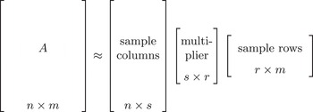
. This is proved in Theorem 2.5. A schematic diagram of
 $C$
,
 $U$
and
 $R$
is shown in Figure 1.1.
Approximating
 $A$
by a sample of
 $s$
columns and
 $r$
rows.

Section 2.3 shows a result based purely on matrix perturbation theory (no probabilities involved) which in words states: If
 $C$
and
 $A$
are any two matrices with
 $CC^{T}\approx AA^{T}$
(
 $C,A$
may be of different dimensions), then the restriction of
 $A$
to the space spanned by the top
 $k$
singular vectors of
 $C$
is a good approximation to
 $A$
. Used in conjunction with (1.1), this reduces the problem of low-rank approximation of
 $A$
to computing the singular value decomposition (SVD) of a submatrix
 $C$
.
In Section 3 we apply length-squared sampling to tensors (higher-dimensional arrays) to obtain good low-rank tensor approximation. Unlike matrices, finding the best low-rank approximation for tensors is NP-hard. Low-rank tensor approximation has several applications, and we show that there is a natural class of tensors (which includes dense hypergraphs and generalizations of metrics) for which, after scaling,
 $\Vert A\Vert _{2}=\unicode[STIX]{x1D6FA}(\Vert A\Vert _{F})$
. Low-rank approximation based on length-squared sampling yields good results.
In Sections 4, 5 and 6 we turn to more refined error bounds for matrices. Can we improve the right-hand side of (1.1) if we want to bound only the spectral norm instead of the Frobenius norm? Using deep results from functional analysis, Rudelson and Vershynin (Reference Rudelson and Vershynin2007) showed that if we use length-squared sampling,
 $$\begin{eqnarray}\displaystyle \Vert CC^{T}-AA^{T}\Vert _{2} & \leq & \displaystyle \unicode[STIX]{x1D700}\Vert A\Vert _{2}\Vert A\Vert _{F}~\text{holds with high probability}\nonumber\\ \displaystyle \text{provided}~s & \geq & \displaystyle \displaystyle \frac{c\ln (1/\unicode[STIX]{x1D700})}{\unicode[STIX]{x1D700}^{2}}.\end{eqnarray}$$
While the change from Frobenius to spectral norm was first considered for its mathematical appeal, it is also suitable for the Hoeffding–Chernoff-type inequality for matrix-valued random variables, proved by Ahlswede and Winter (Reference Ahlswede and Winter2002). We present this theorem and proof (Theorem 4.1), since it is of independent interest. In Section 4 we prove the result of Rudelson and Vershynin.
A central question in probability is to determine how many i.i.d. samples from a probability distribution suffice to make the empirical estimate of the variance close to the true variance in every direction. Mathematically, there is an
 $n\times m$
matrix
 $A$
(with
 $m>n$
,
 $m$
possibly infinite) such that
 $AA^{T}$
is the covariance matrix, and for any unit vector
 $\mathbf{x}\in \mathbb{R}^{n}$
, the variance of the distribution in direction
 $\mathbf{x}$
is
 $\mathbf{x}^{T}AA^{T}\mathbf{x}=|\mathbf{x}^{T}A|^{2}$
. The problem is to find a (small) sample of
 $s$
columns of
 $A$
to form an
 $n\times s$
matrix
 $C$
so that the variance is (approximately) preserved, to relative error
 $\unicode[STIX]{x1D700}$
, in every direction
 $\mathbf{x}$
. That is, we wish to satisfy, for all
 $\mathbf{x}$
,
 $$\begin{eqnarray}\Vert \mathbf{x}^{T}C\Vert ^{2}\in [(1-\unicode[STIX]{x1D700})\Vert \mathbf{x}^{T}A\Vert ^{2},\;(1+\unicode[STIX]{x1D700})\Vert \mathbf{x}^{T}A\Vert ^{2}],\text{ denoted }\Vert \mathbf{x}^{T}C\Vert ^{2}\cong _{\unicode[STIX]{x1D700}}\Vert \mathbf{x}^{T}A\Vert ^{2}.\end{eqnarray}$$
It is important that (1.3) holds simultaneously for all
 $\mathbf{x}$
. It turns out that, in general, if we sample columns of
 $A$
with probability proportional to the squared length not of its own columns but of the columns of
 $A^{+}A$
, where
 $A^{+}$
is the pseudo-inverse of
 $A$
, then (1.3) follows from (1.2). We call this ‘preconditioned’ length-squared sampling (since multiplying
 $A$
by
 $A^{+}$
can be thought of as preconditioning).
There is another, seemingly unrelated context, where exactly the same question (1.3) arises, namely, graph sparsification, considered by Spielman and Srivastava (Reference Spielman and Srivastava2011). Here,
 $A$
is the node–edge signed incidence matrix of a graph, and the goal is to find a subset of edges satisfying (1.3). Spielman and Srivastava (Reference Spielman and Srivastava2011) showed in this case that the squared length of the columns of
 $A^{+}A$
are proportional to the (weighted) electrical resistances and can also be computed in linear time (in the number of edges of the graph).
In theoretical computer science, preconditioned length-squared sampling (also called leverage score sampling) arose from a different motivation: Can the additive error guarantee (1.1) be improved to a relative error guarantee, perhaps with more sophisticated sampling methods? Several answers have been given to this question. The first is simply to iterate length-squared sampling on the residual matrix in the space orthogonal to the span of the sample chosen so far (Deshpande, Rademacher, Vempala and Wang Reference Deshpande, Rademacher, Vempala and Wang2006). Another is to use preconditioned length-squared sampling, where the preconditioning effectively makes the sampling probabilities proportional to the leverage scores (Drineas, Mahoney and Muthukrishnan Reference Drineas, Mahoney and Muthukrishnan2008). A third is volume sampling, which picks a subset of
 $k$
columns with probabilities proportional to the square of the volume of the
 $k$
-simplex they span, together with the origin (Deshpande and Vempala Reference Deshpande and Vempala2006, Deshpande and Rademacher Reference Deshpande and Rademacher2010, Anari, Gharan and Rezaei Reference Anari, Gharan and Rezaei2016). We discuss preconditioned length-squared sampling in Section 5.
In Section 6 we consider an approach pioneered by Clarkson and Woodruff (Reference Clarkson and Woodruff2009, Reference Clarkson and Woodruff2013) for obtaining similar relative-error approximations but in input sparsity time, i.e., time that is asymptotically linear in the number of non-zeros of the input matrix. This is possible via a method known as subspace embedding, which can be performed in linear time using the sparsity of the matrix. We first discuss an inefficient method using random projection, then an efficient method due to Clarkson and Woodruff (Reference Clarkson and Woodruff2013) based on a sparse projection.
As the title of this article indicates, we focus here on randomized algorithms with linear algebra as the important application area. For treatments from a linear algebra perspective (with randomized algorithms as one of the tools), the reader might consult Halko, Martinsson and Tropp (Reference Halko, Martinsson and Tropp2011), Woodruff (Reference Woodruff2014) and references therein.
2 Basic algorithms
2.1 Matrix multiplication using sampling
Suppose
 $A$
is an
 $m\times n$
matrix and
 $B$
is an
 $n\times p$
matrix, and the product
 $AB$
is desired. We can use sampling to get an approximate product faster than the traditional multiplication. Let
 $A(:,k)$
denote the
 $k$
th column of
 $A$
.
 $A(:,k)$
is an
 $m\times 1$
matrix. Let
 $B(k,:)$
be the
 $k$
th row of
 $B$
.
 $B(k,:)$
is a
 $1\times n$
matrix. We have
 $$\begin{eqnarray}AB=\mathop{\sum }_{k=1}^{n}A(:,k)B(k,:).\end{eqnarray}$$
Can we estimate the sum over all
 $k$
by summing over a sub-sample? Let
 $p_{1},p_{2},\ldots ,p_{n}$
be non-negative reals summing to 1 (to be determined later). Let
 $z$
be a random variable that takes values in
 $\{1,2,\ldots ,n\}$
with Pr
 $(z=j)=p_{j}$
. Define an associated matrix random variable
 $X$
such that
 $$\begin{eqnarray}\text{Pr}\biggl(X=\displaystyle \frac{1}{p_{k}}A(:,k)B(k,:)\biggr)=p_{k}.\end{eqnarray}$$
Let
 $E(X)$
denote the entry-wise expectation, that is,
 $$\begin{eqnarray}E(X)=\mathop{\sum }_{k=1}^{n}\text{Pr}(z=k)\displaystyle \frac{1}{p_{k}}A(:,k)B(k,:)=\mathop{\sum }_{k=1}^{n}A(:,k)B(k,:)=AB.\end{eqnarray}$$
The scaling by
 $1/p_{k}$
makes
 $X$
an unbiased estimator of
 $AB$
. We will be interested in
 $E(\Vert AB-X\Vert _{F}^{2})$
, which is just the sum of the variances of all entries of
 $X$
,Footnote
2
since
 $$\begin{eqnarray}\displaystyle E(\Vert AB-X\Vert _{F}^{2}) & = & \displaystyle \mathop{\sum }_{i=1}^{m}\mathop{\sum }_{j=1}^{p}\operatorname{Var}(x_{ij})=\mathop{\sum }_{ij}E(x_{ij}^{2})-E(x_{ij})^{2}\nonumber\\ \displaystyle & = & \displaystyle \biggl(\mathop{\sum }_{ij}\mathop{\sum }_{k}p_{k}\displaystyle \frac{1}{p_{k}^{2}}a_{ik}^{2}b_{kj}^{2}\biggr)-\Vert AB\Vert _{F}^{2}.\nonumber\end{eqnarray}$$
We can ignore the
 $\Vert AB\Vert _{F}^{2}$
term since it does not depend on the
 $p_{k}$
. Now
 $$\begin{eqnarray}\displaystyle \mathop{\sum }_{ij}\mathop{\sum }_{k}p_{k}\displaystyle \frac{1}{p_{k}^{2}}a_{ik}^{2}b_{kj}^{2} & = & \displaystyle \mathop{\sum }_{k}\displaystyle \frac{1}{p_{k}}\biggl(\mathop{\sum }_{i}a_{ik}^{2}\biggr)\biggl(\mathop{\sum }_{j}b_{kj}^{2}\biggr)\nonumber\\ \displaystyle & = & \displaystyle \mathop{\sum }_{k}\displaystyle \frac{1}{p_{k}}|A(:,k)|^{2}|B(k,:)|^{2}.\nonumber\end{eqnarray}$$
It can be seen by calculusFootnote
3
that the minimizing
 $p_{k}$
must be proportional to
 $|A(:,k)\Vert B(k,:)|$
. In the important special case when
 $B=A^{T}$
, this means picking columns of
 $A$
with probabilities proportional to the squared length of the columns. In fact, even in the general case when
 $B\neq A^{T}$
, doing so simplifies the bounds, so we will use it. If
 $p_{k}$
is proportional to
 $|A(:,k)|^{2}$
, that is,
 $$\begin{eqnarray}p_{k}=\displaystyle \frac{|A(:,k)|^{2}}{\Vert A\Vert _{F}^{2}},\end{eqnarray}$$
then
 $$\begin{eqnarray}E(\Vert AB-X\Vert _{F}^{2})=\operatorname{Var}(X)\leq \Vert A\Vert _{F}^{2}\mathop{\sum }_{k}|B(k,:)|^{2}=\Vert A\Vert _{F}^{2}\Vert B\Vert _{F}^{2}.\end{eqnarray}$$
To reduce the variance, we can take the average of
 $s$
independent trials. Each trial
 $i$
,
 $i=1,2,\ldots ,s$
yields a matrix
 $X_{i}$
as in (2.1). We take
 $$\begin{eqnarray}\displaystyle \frac{1}{s}\mathop{\sum }_{i=1}^{s}X_{i}\end{eqnarray}$$
as our estimate of
 $AB$
. Since the variance of the sum of independent random variables is the sum of the variances, we find that
 $$\begin{eqnarray}\operatorname{Var}\biggl(\displaystyle \frac{1}{s}\mathop{\sum }_{i=1}^{s}X_{i}\biggr)=\displaystyle \frac{1}{s}\operatorname{Var}(X)\leq \displaystyle \frac{1}{s}\Vert A\Vert _{F}^{2}\Vert B\Vert _{F}^{2}.\end{eqnarray}$$
Let
 $k_{1},\ldots ,k_{s}$
be the
 $k$
chosen in each trial. Expanding this, we obtain
 $$\begin{eqnarray}\displaystyle \frac{1}{s}\mathop{\sum }_{i=1}^{s}X_{i}=\displaystyle \frac{1}{s}\biggl(\displaystyle \frac{A(:,k_{1})B(k_{1},:)}{p_{k_{1}}}+\displaystyle \frac{A(:,k_{2})B(k_{2},:)}{p_{k_{2}}}+\cdots +\displaystyle \frac{A(:,k_{s})B(k_{s},:)}{p_{k_{s}}}\biggr).\end{eqnarray}$$
We write this as the product of an
 $m\times s$
matrix with an
 $s\times p$
matrix as follows. Let
 $C$
be the
 $m\times s$
matrix consisting of the following columns, which are scaled versions of the chosen columns of
 $A$
:
 $$\begin{eqnarray}\displaystyle \frac{A(:,k_{1})}{\sqrt{sp_{k_{1}}}},\quad \displaystyle \frac{A(:,k_{2})}{\sqrt{sp_{k_{2}}}},\ldots ,\displaystyle \frac{A(:,k_{s})}{\sqrt{sp_{k_{s}}}}.\end{eqnarray}$$
Note that this scaling has a nice property, which we leave to the reader to verify:
 $$\begin{eqnarray}E(CC^{T})=AA^{T}.\end{eqnarray}$$
Define
 $R$
to be the
 $s\times p$
matrix with the corresponding rows of
 $B$
similarly scaled, namely,
 $R$
has rows
 $$\begin{eqnarray}\displaystyle \frac{B(k_{1},:)}{\sqrt{sp_{k_{1}}}},\quad \displaystyle \frac{B(k_{2},:)}{\sqrt{sp_{k_{2}}}},\ldots ,\displaystyle \frac{B(k_{s},:)}{\sqrt{sp_{k_{s}}}}.\end{eqnarray}$$
The reader may also verify that
 $$\begin{eqnarray}E(R^{T}R)=A^{T}A.\end{eqnarray}$$
From (2.2), we see that
 $$\begin{eqnarray}\displaystyle \frac{1}{s}\mathop{\sum }_{i=1}^{s}X_{i}=CR.\end{eqnarray}$$
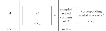
This is represented in Figure 2.1. We summarize our discussion in Theorem 2.1.
Approximate matrix multiplication using sampling.

Theorem 2.1. Suppose
 $A$
is an
 $m\times n$
matrix and
 $B$
is an
 $n\times p$
matrix. The product
 $AB$
can be estimated by
 $CR$
, where
 $C$
is an
 $m\times s$
matrix consisting of
 $s$
columns of
 $A$
picked according to length-squared distribution and scaled to satisfy (2.3), and
 $R$
is the
 $s\times p$
matrix consisting of the corresponding rows of
 $B$
scaled to satisfy (2.4). The error is bounded by
 $$\begin{eqnarray}E(\Vert AB-CR\Vert _{F}^{2})\leq \displaystyle \frac{\Vert A\Vert _{F}^{2}\;\Vert B\Vert _{F}^{2}}{s}.\end{eqnarray}$$
Thus, to ensure that
 $$\begin{eqnarray}E(\Vert AB-CR\Vert _{F}^{2})\leq \unicode[STIX]{x1D700}^{2}\Vert A\Vert _{F}^{2}\Vert B\Vert _{F}^{2},\end{eqnarray}$$
it suffices to choose
 $s\geq 1/\unicode[STIX]{x1D700}^{2}$
. If now
 $\unicode[STIX]{x1D700}=\unicode[STIX]{x1D6FA}(1)$
(and so
 $s=O(1)$
), then the multiplication
 $CR$
can be carried out in time
 $O(mp)$
.
When is this the error bound useful? Let us focus on the case
 $B=A^{T}$
so that we have just one matrix to consider. If
 $A$
is the identity matrix, then the guarantee is not very good. In this case,
 $\Vert AA^{T}\Vert _{F}^{2}=n$
, but the right-hand side of the inequality is
 $n^{2}/s$
. So we would need
 $s>n$
for the bound to be any better than approximating the product with the zero matrix.
More generally, the trivial estimate of the zero matrix for
 $AA^{T}$
makes an error in the Frobenius norm of
 $\Vert AA^{T}\Vert _{F}$
. If
 $\unicode[STIX]{x1D70E}_{1},\unicode[STIX]{x1D70E}_{2},\ldots$
are the singular values of
 $A$
, then the singular values of
 $AA^{T}$
are
 $\unicode[STIX]{x1D70E}_{1}^{2},\unicode[STIX]{x1D70E}_{2}^{2},\ldots ,$
and we have
 $$\begin{eqnarray}\Vert A\Vert _{F}^{2}=\mathop{\sum }_{t}\unicode[STIX]{x1D70E}_{t}^{2}\quad \text{and}\quad \Vert AA^{T}\Vert _{F}^{2}=\mathop{\sum }_{t}\unicode[STIX]{x1D70E}_{t}^{4}.\end{eqnarray}$$
So from the theorem we can assert
 $$\begin{eqnarray}E(\Vert AA^{T}-CR\Vert _{F}^{2})\leq \Vert AA^{T}\Vert _{F}^{2}\end{eqnarray}$$
provided that
 $$\begin{eqnarray}s\geq \displaystyle \frac{(\unicode[STIX]{x1D70E}_{1}^{2}+\unicode[STIX]{x1D70E}_{2}^{2}+\cdots )^{2}}{\unicode[STIX]{x1D70E}_{1}^{4}+\unicode[STIX]{x1D70E}_{2}^{4}+\cdots }.\end{eqnarray}$$
If
 $\operatorname{rank}(A)=r$
, then there are
 $r$
non-zero
 $\unicode[STIX]{x1D70E}_{t}$
and the best general upper bound on the ratio
 $(\unicode[STIX]{x1D70E}_{1}^{2}+\unicode[STIX]{x1D70E}_{2}^{2}+\cdots )^{2}/(\unicode[STIX]{x1D70E}_{1}^{4}+\unicode[STIX]{x1D70E}_{2}^{4}+\cdots )$
is
 $r$
, so in general,
 $s$
needs to be at least
 $r$
. If
 $A$
is of full rank, this means that sampling will not give us any gain over taking the whole matrix!
However, if there is a constant
 $c$
and a small integer
 $p$
such that
 $$\begin{eqnarray}\unicode[STIX]{x1D70E}_{1}^{2}+\unicode[STIX]{x1D70E}_{2}^{2}+\cdots +\unicode[STIX]{x1D70E}_{p}^{2}\geq c(\unicode[STIX]{x1D70E}_{1}^{2}+\unicode[STIX]{x1D70E}_{2}^{2}+\cdots +\unicode[STIX]{x1D70E}_{r}^{2}),\end{eqnarray}$$
then
 $$\begin{eqnarray}\displaystyle \frac{(\unicode[STIX]{x1D70E}_{1}^{2}+\unicode[STIX]{x1D70E}_{2}^{2}+\cdots +\unicode[STIX]{x1D70E}_{r}^{2})^{2}}{\unicode[STIX]{x1D70E}_{1}^{4}+\unicode[STIX]{x1D70E}_{2}^{4}+\cdots +\unicode[STIX]{x1D70E}_{r}^{4}}\leq \displaystyle \frac{1}{c^{2}}\displaystyle \frac{(\unicode[STIX]{x1D70E}_{1}^{2}+\unicode[STIX]{x1D70E}_{2}^{2}+\cdots +\unicode[STIX]{x1D70E}_{p}^{2})^{2}}{\unicode[STIX]{x1D70E}_{1}^{4}+\unicode[STIX]{x1D70E}_{2}^{4}+\cdots +\unicode[STIX]{x1D70E}_{p}^{2}}\leq \displaystyle \frac{p}{c^{2}},\end{eqnarray}$$
and so
 $s\geq p/c^{2}$
gives us a better estimate than the zero matrix. Further increasing
 $s$
by a factor decreases the error by the same factor. The condition (2.5) (in words, the top
 $p$
singular values make up a constant fraction of the spectrum) is indeed the hypothesis of the subject of principal component analysis, and there are many situations when the data matrix does satisfy the condition and so sampling algorithms are useful.
2.1.1 Implementing length-squared sampling in two passes
Traditional matrix algorithms often assume that the input matrix is in random access memory (RAM) and so any particular entry of the matrix can be accessed in unit time. For massive matrices, RAM may be too small to hold the entire matrix, but may be able to hold and compute with the sampled columns/rows.
Let us consider a high-level model where the input matrix or matrices have to be read from ‘external memory’ using a ‘pass’. In one pass, we can read sequentially all entries of the matrix in some order. We may do some ‘sampling on the fly’ as the pass is going on.
It is easy to see that two passes suffice to draw a sample of columns of
 $A$
according to length-squared probabilities, even if the matrix is not in row order or column order and entries are presented as a linked list (as in sparse representations). In the first pass, we just compute the squared length of each column and store this information in RAM. The squared lengths can be computed as running sums. Then, we use a random number generator in RAM to figure out the columns to be sampled (according to length-squared probabilities). Then, we make a second pass in which we pick out the columns to be sampled.
What if the matrix is already presented in external memory in column order? In this case, one pass will do, based on a primitive using rejection sampling.
The primitive is as follows. We are given a stream (i.e. a read-once only input sequence) of positive real numbers
 $a_{1},a_{2},\ldots ,a_{n}$
. We seek to have a random
 $i\in \{1,2,\ldots ,n\}$
at the end, with the property that the probability of choosing
 $i$
is exactly equal to
 $a_{i}/\sum _{j=1}^{n}a_{j}$
, for all
 $i$
. This is solved as follows. After having read
 $a_{1},a_{2},\ldots ,a_{i}$
, suppose we have (i)
 $\sum _{j=1}^{i}a_{j}$
and (ii) a sample
 $a_{j},j\leq i$
, picked with probability
 $a_{j}/\sum _{k=1}^{i}a_{k}$
. On reading
 $a_{i+1}$
, we update the sum and, with the correct probability, reject the earlier sample and replace it with
 $a_{i+1}$
. If we need
 $s$
independent identical samples, we just run
 $s$
such processes in parallel.
2.2 Sketch of a large matrix
The main result of this section is that for any matrix, a sample of columns and rows, each picked according to length-squared distribution, provides a good sketch of the matrix in a formal sense that will be described briefly. Let
 $A$
be an
 $m\times n$
matrix. Pick
 $s$
columns of
 $A$
according to length-squared distribution. Let
 $C$
be the
 $m\times s$
matrix containing the picked columns scaled so as to satisfy (2.3), that is, if
 $A(:,k)$
is picked, it is scaled by
 $1/\sqrt{sp_{k}}$
. Similarly, pick
 $r$
rows of
 $A$
according to length-squared distribution on the rows of
 $A$
. Let
 $R$
be the
 $r\times n$
matrix of the picked rows, scaled as follows. If row
 $k$
of
 $A$
is picked, it is scaled by
 $1/\sqrt{rp_{k}}$
. We then have
 $E(R^{T}R)=A^{T}A$
. From
 $C$
and
 $R$
, we can find a matrix
 $U$
so that
 $A\approx CUR$
.
One may recall that the top
 $k$
singular vectors give a similar picture. But the SVD takes more time to compute, requires all of
 $A$
to be stored in RAM, and does not have the property that the singular vectors, the basis of the reduced space, are directly from
 $A$
. The last property – that the approximation involves actual rows/columns of the matrix rather than linear combinations – is called an interpolative approximation, and is useful in many contexts. Some structural results of such approximations are found in the work of Stewart (Stewart Reference Stewart1999, Stewart Reference Stewart2004, Berry, Pulatova and Stewart Reference Berry, Pulatova and Stewart2004) and Goreinov, Tyrtyshnikov and Zamarashkin (Goreinov, Tyrtyshnikov and Zamarashkin Reference Goreinov, Tyrtyshnikov and Zamarashkin1997, Goreinov and Tyrtyshnikov Reference Goreinov and Tyrtyshnikov2001).
We briefly mention two motivations for such a sketch. Suppose
 $A$
is the document-term matrix of a large collection of documents. We are to ‘read’ the collection at the outset and store a sketch so that later, when a query represented by a vector with one entry per term arrives, we can find its similarity to each document in the collection. Similarity is defined by the dot product. In Figure 1.1 it is clear that the matrix–vector product of a query with the right-hand side can be done in time
 $O(ns+sr+rm)$
, which would be linear in
 $n$
and
 $m$
if
 $s$
and
 $r$
are
 $O(1)$
. To bound errors for this process, we need to show that the difference between
 $A$
and the sketch of
 $A$
has small 2-norm. The fact that the sketch is an interpolative approximation means that our approximation essentially consists a subset of documents and a subset of terms, which may be thought of as a representative set of documents and terms. Moreover, if
 $A$
is sparse in its rows and columns – each document contains only a small fraction of the terms and each term is in only a small fraction of the documents – then this property will be preserved in
 $C$
and
 $R$
, unlike with the SVD.
A second motivation comes from recommendation systems. Here
 $A$
would be a customer–product matrix whose
 $(i,j)$
th entry is the preference of customer
 $i$
for product
 $j$
. The objective is to collect a few sample entries of
 $A$
and, based on these, get an approximation to
 $A$
so that we can make future recommendations. A few sampled rows of
 $A$
(all preferences of a few customers) and a few sampled columns (all customer preferences for a few products) give a good approximation to
 $A$
provided that the samples are drawn according to the length-squared distribution.
It now remains to describe how to find
 $U$
from
 $C$
and
 $R$
. There is an
 $n\times n$
matrix
 $P$
of the form
 $P=QR$
which acts as the identity on the space spanned by the rows of
 $R$
and zeros out all vectors orthogonal to this space. The matrix
 $Q$
is just the pseudo-inverse of
 $R$
.
Lemma 2.2. If
 $\operatorname{rank}(R)=r^{\prime }$
and
 $R=\sum _{t=1}^{r^{\prime }}\unicode[STIX]{x1D70E}_{t}\mathbf{u}_{t}\mathbf{v}_{t}^{T}$
is the SVD of
 $R$
, then the matrix
 $P=(\sum _{t=1}^{r^{\prime }}{\unicode[STIX]{x1D70E}_{t}}^{-1\,}\mathbf{v}_{t}\mathbf{u}_{t}^{T})R$
satisfies:
-
(i)
$P\mathbf{x}=\mathbf{x}$
for every vector
$\mathbf{x}$
of the form
$\mathbf{x}=R^{T}\mathbf{y}$
, -
(ii) if
$\mathbf{x}$
is orthogonal to the row space of
$R$
, then
$P\mathbf{x}=\mathbf{0}$
, -
(iii)
$P=R^{T}(\sum _{t=1}^{r^{\prime }}{\unicode[STIX]{x1D70E}_{t}}^{-2\,}\mathbf{u}_{t}\mathbf{u}_{t}^{T})R.$


We begin with some intuition. In particular, we first present a simpler idea that does not work but will then motivate the idea that does work. Write
 $A$
as
 $AI$
, where
 $I$
is the
 $n\times n$
identity matrix. Now, let us approximate the product
 $AI$
using the algorithm of Theorem 2.1 from the previous section, that is, by sampling
 $s$
columns of
 $A$
according to their squared lengths. Then, as in the last section, write
 $AI\approx CW$
, where
 $W$
consists of a scaled version of the
 $s$
rows of
 $I$
corresponding to the
 $s$
columns of
 $A$
that were picked. Theorem 2.1 bounds the error
 $\Vert A-CW\Vert _{F}^{2}$
by
 $$\begin{eqnarray}\Vert A\Vert _{F}^{2}\Vert I\Vert _{F}^{2}/s=\Vert A\Vert _{F}^{2}\displaystyle \frac{n}{s}.\end{eqnarray}$$
But we would like the error to be a small fraction of
 $\Vert A\Vert _{F}^{2}$
which would require
 $s\geq n$
, which clearly is of no use since this would pick at least as many columns as the whole of
 $A$
.
Instead, let us use the identity-like matrix
 $P$
instead of
 $I$
in the above discussion. Using the fact that
 $R$
is picked according to the squared length, we will show the following proposition later.
Proposition 2.3.
 $A\approx AP$
with error
 $E(\Vert A-AP\Vert _{2}^{2})\leq \Vert A\Vert _{F}^{2}/\sqrt{r}$
.
We then use Theorem 2.1 to argue that instead of doing the multiplication
 $AP$
, we can use the sampled columns of
 $A$
and the corresponding rows of
 $P$
. The sampled
 $s$
columns of
 $A$
form
 $C$
. We have to take the corresponding
 $s$
rows of the matrix
 $$\begin{eqnarray}P=R^{T}\;\biggl(\mathop{\sum }_{t=1}^{r^{\prime }}\displaystyle \frac{1}{\unicode[STIX]{x1D70E}_{t}^{2}}\mathbf{u}_{t}\mathbf{u}_{t}^{T}\biggr)\;R.\end{eqnarray}$$
This is the same as taking the corresponding
 $s$
rows of
 $R^{T}$
and multiplying this by
 $(\sum _{t=1}^{r^{\prime }}{\unicode[STIX]{x1D70E}_{t}}^{-2\,}\mathbf{u}_{t}\mathbf{u}_{t}^{T})R.$
It is easy to check that this leads to an expression of the form
 $CUR$
. Moreover, by Theorem 2.1, the error is bounded by
 $$\begin{eqnarray}E(\Vert AP-CUR\Vert _{2}^{2})\leq E(\Vert AP-CUR\Vert _{F}^{2})\leq \displaystyle \frac{\Vert A\Vert _{F}^{2}\Vert P\Vert _{F}^{2}}{s}\leq \displaystyle \frac{r}{s}\Vert A\Vert _{F}^{2},\end{eqnarray}$$
since we will deduce the following inequality.
Proposition 2.4.
 $\Vert P\Vert _{F}^{2}\leq r.$
Combining (2.6) and Proposition 2.3, and using the fact that by the triangle inequality we have
 $$\begin{eqnarray}\Vert A-CUR\Vert _{2}\leq \Vert A-AP\Vert _{2}+\Vert AP-CUR\Vert _{2},\end{eqnarray}$$
which in turn implies that
 $$\begin{eqnarray}\Vert A-CUR\Vert _{2}^{2}\leq 2\Vert A-AP\Vert _{2}^{2}+2\Vert AP-CUR\Vert _{2}^{2},\end{eqnarray}$$
we obtain the main result.
Theorem 2.5. Suppose
 $A$
is any
 $m\times n$
matrix and
 $r$
and
 $s$
are positive integers. Suppose
 $C$
is an
 $m\times s$
matrix of
 $s$
columns of
 $A$
picked according to length-squared sampling, and similarly
 $R$
is a matrix of
 $r$
rows of
 $A$
picked according to length-squared sampling. Then we can find from
 $C,R$
an
 $s\times r$
matrix
 $U$
such that
 $$\begin{eqnarray}E(\Vert A-CUR\Vert _{2}^{2})\leq \Vert A\Vert _{F}^{2}\biggl(\displaystyle \frac{2}{\sqrt{r}}+\displaystyle \frac{2r}{s}\biggr).\end{eqnarray}$$
We see that if
 $s$
is fixed, the error is minimized when
 $r=(s/2)^{2/3}$
. Choosing
 $s=O(r/\unicode[STIX]{x1D700})$
and
 $r=1/\unicode[STIX]{x1D700}^{2}$
, the bound becomes
 $O(\unicode[STIX]{x1D700})\Vert A\Vert _{F}^{2}$
.
Now we prove Proposition 2.3. First,
 $$\begin{eqnarray}\Vert A-AP\Vert _{2}^{2}=\max _{\{\mathbf{x}:|\mathbf{x}|=1\}}|(A-AP)\mathbf{x}|^{2}.\end{eqnarray}$$
Let us first suppose that
 $\mathbf{x}$
is in the row space
 $V$
of
 $R$
. We have
 $P\mathbf{x}=\mathbf{x}$
, so for
 $\mathbf{x}\in V$
we have
 $(A-AP)\mathbf{x}=\mathbf{0}$
. Now, since every vector can be written as the sum of a vector in
 $V$
plus a vector orthogonal to
 $V$
, this implies that the maximum must therefore occur at some
 $\mathbf{x}\in V^{\bot }$
. For such
 $\mathbf{x}$
, we have
 $(A-AP)\mathbf{x}=A\mathbf{x}$
. Thus, the question now becomes: For unit-length
 $\mathbf{x}\in V^{\bot }$
, how large can
 $\Vert A\mathbf{x}\Vert ^{2}$
be? To analyse this, we can write
 $$\begin{eqnarray}\displaystyle \Vert A\mathbf{x}\Vert ^{2} & = & \displaystyle \mathbf{x}^{T}A^{T}A\mathbf{x}=\mathbf{x}^{T}(A^{T}A-R^{T}R)\mathbf{x}\nonumber\\ \displaystyle & \leq & \displaystyle \Vert A^{T}A-R^{T}R\Vert _{2}|\mathbf{x}|^{2}\leq \Vert A^{T}A-R^{T}R\Vert _{2}.\nonumber\end{eqnarray}$$
This implies that we get
 $\Vert A-AP\Vert _{2}^{2}\leq \Vert A^{T}A-R^{T}R\Vert _{2}$
. So, it suffices to prove that
 $$\begin{eqnarray}E(\Vert A^{T}A-R^{T}R\Vert _{2}^{2})\leq \Vert A\Vert _{F}^{4}/r,\end{eqnarray}$$
which follows directly from Theorem 2.1, since we can think of
 $R^{T}R$
as a way of estimating
 $A^{T}A$
by picking (according to length-squared distribution) columns of
 $A^{T}$
, that is, rows of
 $A$
. By Jensen’s inequality, this implies that
 $$\begin{eqnarray}E(\Vert A^{T}A-R^{T}R\Vert _{2})\leq \displaystyle \frac{\Vert A\Vert _{F}^{2}}{\sqrt{r}}\end{eqnarray}$$
and proves Proposition 2.3.
Proposition 2.4 is easy to see. Since, by Lemma 2.2,
 $P$
is the identity on the space
 $V$
spanned by the rows of
 $R$
, and
 $P\mathbf{x}=0$
for
 $\mathbf{x}$
perpendicular to the rows of
 $R$
, we have that
 $\Vert P\Vert _{F}^{2}$
is the sum of its singular values squared, which is at most
 $r$
as claimed.
Finally, to bound the time needed to compute
 $U$
, the only step involved in computing
 $U$
is to find the SVD of
 $R$
. But note that
 $RR^{T}$
is an
 $r\times r$
matrix, and since
 $r$
is much smaller than
 $n,m$
, this is fast.
2.3 Low-rank approximations and the SVD
Singular value decomposition yields the best approximation of given rank to a matrix in both spectral norm and Frobenius norm. Here, we show that a near-optimal low-rank approximation (LRA) of a matrix
 $A$
can be found by computing the SVD of a smaller matrix
 $R$
. The main result is that for any matrix
 $R$
with
 $$\begin{eqnarray}A^{T}A\approx R^{T}R,\end{eqnarray}$$
the restriction of
 $A$
to the space spanned by the top few right singular vectors of
 $R$
is a good approximation to
 $A$
. This is purely based on matrix perturbation theory: there is no probability involved.
If we can find an
 $R$
with smaller dimensions than
 $A$
, with
 $R^{T}R\approx A^{T}A$
, then computing the SVD for
 $R$
would be faster. Indeed, we have already seen one way of getting such an
 $R$
: pick a set of
 $r$
rows of
 $A$
in
 $r$
i.i.d. trials according to the length-squared distribution and scale them so that
 $E(R^{T}R)=A^{T}A$
. We saw in Theorem 2.1 that
 $R^{T}R\approx A^{T}A$
.
The Hoffman–Wielandt inequality (stated below) implies that if
 $\Vert R^{T}R-A^{T}A\Vert _{F}$
is small, then the singular values of
 $A$
and
 $R$
are close. If the top singular vectors of
 $R$
and
 $A$
were close, the desired result would follow easily. However, as is well known, multiple singular values are points of discontinuity of singular vectors. But it is not difficult to see intuitively that LRA is not discontinuous: using a singular vector of a slightly worse singular value does not induce gross errors in LRA, and this intuition underlies the result proved formally here.
2.3.1 Restriction to the SVD subspace
If
 $\mathbf{w}_{1},\mathbf{w}_{2},\ldots ,\mathbf{w}_{k}$
is a basis for the vector space
 $V$
, the restriction of
 $A$
to
 $V$
is
 $$\begin{eqnarray}\bar{A}=A\mathop{\sum }_{t=1}^{k}\mathbf{w}_{t}\mathbf{w}_{t}^{T}~\text{satisfies}~\bar{A}\mathbf{x}=\left\{\begin{array}{@{}ll@{}}A\mathbf{x}\quad & \text{if}~x\in V,\\ 0\quad & \text{if}~\mathbf{x}\bot V.\end{array}\right.\end{eqnarray}$$
Theorem 2.6. For any
 $r\times n$
matrix
 $R$
and any
 $m\times n$
matrix
 $A$
, if
 $\mathbf{v}_{1},\mathbf{v}_{2},\ldots ,\mathbf{v}_{k}$
are the top
 $k$
right singular vectors of
 $R$
and
 $A(k)$
is the best rank-
 $k$
approximation to
 $A$
, then
 $$\begin{eqnarray}\displaystyle \biggl\|A-A\mathop{\sum }_{t=1}^{k}\mathbf{v}_{t}\mathbf{v}_{t}^{T}\biggr\|_{F}^{2} & \leq & \displaystyle \Vert A-A(k)\Vert _{F}^{2}+2\sqrt{k}\Vert R^{T}R-A^{T}A\Vert _{F},\end{eqnarray}$$
 $$\begin{eqnarray}\displaystyle \biggl\|A-A\mathop{\sum }_{t=1}^{k}\mathbf{v}_{t}\mathbf{v}_{t}^{T}\biggr\|_{2}^{2} & \leq & \displaystyle \Vert A-A(k)\Vert _{2}^{2}+2\Vert R^{T}R-A^{T}A\Vert _{2}.\end{eqnarray}$$
In (2.8), the first term
 $\Vert A-A(k)\Vert _{F}^{2}$
is the best possible error we can make with exact SVD of
 $A$
. We cannot avoid that. The second term is the penalty we pay for computing with
 $R$
instead of
 $A$
, and similarly for (2.9). The theorem is for any
 $r$
including the cases
 $r=0$
and
 $r=n$
. Central to the proof is the Hoffman–Wielandt inequality, stated next without proof.
Lemma 2.7. If
 $P,Q$
are two real symmetric
 $n\times n$
matrices and
 $\unicode[STIX]{x1D706}_{1},\unicode[STIX]{x1D706}_{2},\ldots$
denote eigenvalues in non-increasing order, then
 $$\begin{eqnarray}\mathop{\sum }_{t=1}^{n}(\unicode[STIX]{x1D706}_{t}(P)-\unicode[STIX]{x1D706}_{t}(Q))^{2}\leq \Vert P-Q\Vert _{F}^{2}.\end{eqnarray}$$
We can now prove the low-rank approximation guarantee.
Proof of Theorem 2.6.
Complete
 $\mathbf{v}_{1},\mathbf{v}_{2},\ldots ,\mathbf{v}_{k}$
to a basis
 $\mathbf{v}_{1},\mathbf{v}_{2},\ldots ,\mathbf{v}_{n}$
of
 $\mathbb{R}^{n}$
. Then
 $$\begin{eqnarray}\displaystyle & & \displaystyle \biggl\|A-A\mathop{\sum }_{t=1}^{k}\mathbf{v}_{t}\mathbf{v}_{t}^{T}\biggr\|_{F}^{2}-\Vert A-A(k)\Vert _{F}^{2}\nonumber\\ \displaystyle & & \displaystyle \qquad =\Vert A\Vert _{F}^{2}-\biggl\|A\mathop{\sum }_{t=1}^{k}\mathbf{v}_{t}\mathbf{v}_{t}^{T}\biggr\|_{F}^{2}-(\Vert A\Vert _{F}^{2}-\Vert A(k)\Vert _{F}^{2})\nonumber\\ \displaystyle & & \displaystyle \qquad =\Vert A(k)\Vert _{F}^{2}-\biggl\|A\mathop{\sum }_{t=1}^{k}\mathbf{v}_{t}\mathbf{v}_{t}^{T}\biggr\|_{F}^{2}\nonumber\\ \displaystyle & & \displaystyle \qquad =\mathop{\sum }_{t=1}^{k}\unicode[STIX]{x1D70E}_{t}^{2}(A)-\mathop{\sum }_{t=1}^{k}\Vert A\mathbf{v}_{t}\Vert ^{2}\nonumber\\ \displaystyle & & \displaystyle \qquad =\mathop{\sum }_{t=1}^{k}\unicode[STIX]{x1D70E}_{t}^{2}(A)-\mathop{\sum }_{t=1}^{k}\mathbf{v}_{t}^{T}(A^{T}A-R^{T}R)\mathbf{v}_{t}-\mathop{\sum }_{t=1}^{k}\mathbf{v}_{t}^{T}R^{T}R\mathbf{v}_{t}\nonumber\\ \displaystyle & & \displaystyle \qquad =\mathop{\sum }_{t=1}^{k}(\unicode[STIX]{x1D70E}_{t}^{2}(A)-\unicode[STIX]{x1D70E}_{t}^{2}(R))-\mathop{\sum }_{t=1}^{k}\mathbf{v}_{t}^{T}(A^{T}A-R^{T}R)\mathbf{v}_{t}.\nonumber\end{eqnarray}$$
We can now deduce that
 $$\begin{eqnarray}\biggl|\mathop{\sum }_{t=1}^{k}\mathbf{v}_{t}^{T}(A^{T}A-R^{T}R)\mathbf{v}_{t}\biggr|\leq k\Vert A^{T}A-R^{T}R\Vert _{2},\end{eqnarray}$$
but we want
 $\sqrt{k}$
instead of
 $k$
. For this, we use the Cauchy–Schwarz inequality to assert
 $$\begin{eqnarray}\displaystyle \biggl|\mathop{\sum }_{t=1}^{k}\mathbf{v}_{t}^{T}(A^{T}A-R^{T}R)\mathbf{v}_{t}\biggr| & \leq & \displaystyle \sqrt{k}\biggl(\mathop{\sum }_{t=1}^{k}(\mathbf{v}_{t}^{T}(A^{T}A-R^{T}R)\mathbf{v}_{t})^{2}\biggr)^{1/2}\nonumber\\ \displaystyle & \leq & \displaystyle \sqrt{k}\Vert A^{T}A-R^{T}R\Vert _{F},\nonumber\end{eqnarray}$$
since the Frobenius norm is invariant under change of basis and, in a basis containing
 $\mathbf{v}_{1},\mathbf{v}_{2},\ldots ,\mathbf{v}_{k}$
,
 $$\begin{eqnarray}\mathop{\sum }_{t=1}^{k}(\mathbf{v}_{t}^{T}(A^{T}A-R^{T}R)\mathbf{v}_{t})^{2}\end{eqnarray}$$
is the sum of squares of the first
 $k$
diagonal entries of
 $A^{T}A-R^{T}R$
. We still have to bound
 $$\begin{eqnarray}\mathop{\sum }_{t=1}^{k}(\unicode[STIX]{x1D70E}_{t}^{2}(A)-\unicode[STIX]{x1D70E}_{t}^{2}(R)),\end{eqnarray}$$
for which we use the Hoffman–Wielandt inequality, after another use of Cauchy–Schwarz:
 $$\begin{eqnarray}\mathop{\sum }_{t=1}^{k}(\unicode[STIX]{x1D70E}_{t}^{2}(A)-\unicode[STIX]{x1D70E}_{t}^{2}(R))\leq \sqrt{k}\biggl(\mathop{\sum }_{t=1}^{k}(\unicode[STIX]{x1D70E}_{t}^{2}(A)-\unicode[STIX]{x1D70E}_{t}^{2}(R))^{2}\biggr)^{1/2}.\end{eqnarray}$$
Now
 $\unicode[STIX]{x1D70E}_{t}^{2}(A)=\unicode[STIX]{x1D706}_{t}(A^{T}A)$
and
 $\unicode[STIX]{x1D70E}_{t}^{2}(R)=\unicode[STIX]{x1D706}_{t}(R^{T}R)$
, and so
 $$\begin{eqnarray}\mathop{\sum }_{t=1}^{k}(\unicode[STIX]{x1D70E}_{t}^{2}(A)-\unicode[STIX]{x1D70E}_{t}^{2}(R))^{2}\leq \Vert A^{T}A-R^{T}R\Vert _{F}^{2}.\end{eqnarray}$$
Plugging these in, we obtain (2.8).
For (2.9), first note that the top singular vector
 $\mathbf{u}$
of
 $A-A\sum _{t=1}^{k}\mathbf{v}_{t}\mathbf{v}_{t}^{T}$
must be orthogonal to the span of
 $\mathbf{v}_{1},\mathbf{v}_{2},\ldots ,\mathbf{v}_{k}$
. Hence
 $$\begin{eqnarray}\biggl(A-A\mathop{\sum }_{t=1}^{k}\mathbf{v}_{t}\mathbf{v}_{t}^{T}\biggr)\mathbf{u}=A\mathbf{u}\end{eqnarray}$$
by (2.7). Thus
 $$\begin{eqnarray}\displaystyle & & \displaystyle \biggl\|A-A\mathop{\sum }_{t=1}^{k}\mathbf{v}_{t}\mathbf{v}_{t}^{T}\biggr\|_{2}^{2}\nonumber\\ \displaystyle & & \displaystyle \qquad =\Vert A\mathbf{u}\Vert ^{2}\nonumber\\ \displaystyle & & \displaystyle \qquad =\mathbf{u}^{T}A^{T}A\mathbf{u}\nonumber\\ \displaystyle & & \displaystyle \qquad =\mathbf{u}^{T}(A^{T}A-R^{T}R)\mathbf{u}+\mathbf{u}^{T}R^{T}R\mathbf{u}\leq \Vert A^{T}A-R^{T}R\Vert _{2}+\unicode[STIX]{x1D70E}_{k+1}^{2}(R)\nonumber\\ \displaystyle & & \displaystyle \qquad =\Vert A^{T}A-R^{T}R\Vert _{2}+(\unicode[STIX]{x1D70E}_{k+1}^{2}(R)-\unicode[STIX]{x1D70E}_{k+1}^{2}(A))+\unicode[STIX]{x1D70E}_{k+1}^{2}(A)\nonumber\\ \displaystyle & & \displaystyle \qquad \leq 2\Vert A^{T}A-R^{T}R\Vert _{2}+\unicode[STIX]{x1D70E}_{k+1}^{2}(A),\nonumber\end{eqnarray}$$
by Weyl’s inequality (Horn and Johnson Reference Horn and Johnson2012, Section 4.3), which states that
 $$\begin{eqnarray}\unicode[STIX]{x1D706}_{k+1}(R^{T}R)\in [\unicode[STIX]{x1D706}_{k+1}(A^{T}A)-\Vert A^{T}A-R^{T}R\Vert _{2},\;\unicode[STIX]{x1D706}_{k+1}(A^{T}A)+\Vert A^{T}A-R^{T}R\Vert _{2}].\end{eqnarray}$$
To summarize, here is the algorithm for LRA of
 $A$
after one final note: we need the right singular vectors of
 $R$
. For this, we can compute the SVD of
 $RR^{T}$
(an
 $r\times r$
matrix) to find the left singular vectors of
 $R$
, from which we can get the right singular vectors.
-
(1) Pick
$r$
rows of
$A$
by length-squared sampling, and scale them so that for the resulting
$r\times n$
matrix
$R$
,
$E(R^{T}R)=A^{T}A$
. -
(2) Find
$RR^{T}$
. Find the left singular vectors of
$R$
by computing the SVD of the
$r\times r$
matrix
$RR^{T}$
. Premultiply
$R$
by the left singular vectors to get the right singular vectors
$\mathbf{v}_{1},\mathbf{v}_{2},\ldots ,\mathbf{v}_{k}$
of
$R$
. -
(3) Return
$A\sum _{t=1}\mathbf{v}_{t}\mathbf{v}_{t}^{T}$
as the implicit LRA (or if required, multiply out and return the matrix).


Let
 $p$
be the maximum number of non-zero entries in any row of
 $A$
(
 $p\leq n$
). The first step can be done in two passes from external memory. For the second step,
 $RR^{T}$
can be found in
 $O(r^{2}p)$
time. The spectral decomposition of
 $RR^{T}$
can be done in time
 $O(r^{3})$
(or better). Finally, multiplying the
 $k$
left singular values by
 $R$
can be done in time
 $O(krp)$
.
The running time has been improved by Drineas, Kannan and Mahoney (Reference Drineas, Kannan and Mahoney2006) and further by Clarkson and Woodruff (see Woodruff Reference Woodruff2014).
3 Tensor approximation via length-squared sampling
An
 $r$
-tensor
 $A$
is an
 $r$
-dimensional array with real entries
 $A_{i_{1},i_{2},\ldots ,i_{r}}$
, for
 $i_{1},i_{2},\ldots ,i_{r}\in \{1,2,\ldots ,n\}$
. Tensors encode mutual information about subsets of size three or higher (matrix entries are pairwise information) and arise naturally in a number of applications.
In analogy with matrices, we may define a rank-
 $1$
tensor to be the outer product of
 $r$
vectors
 $\mathbf{x}^{(1)},\mathbf{x}^{(2)},\ldots ,\mathbf{x}^{(r)}$
denoted
 $\mathbf{x}^{(1)}\otimes \mathbf{x}^{(2)}\otimes \cdots \otimes \mathbf{x}^{(r)}$
, with
 $(i_{1},i_{2},\ldots ,i_{r})$
th entry
 $x_{i_{1}}^{(1)}x_{i_{2}}^{(2)}\cdots x_{i_{r}}^{(r)}$
. We will show the following.
-
(1) For any
$r$
-tensor
$A$
, there exists a good approximation by the sum of a small number of rank-1 tensors (Lemma 3.2). -
(2) We can algorithmically find such an approximation (Theorem 3.3).


In the case of matrices, traditional linear algebra algorithms find optimal approximations in polynomial time. Unfortunately, there is no such theory (or algorithm) for
 $r$
-dimensional arrays when
 $r>2$
. Indeed, there are computational hardness results (Hillar and Lim Reference Hillar and Lim2013). But our focus here is what we can do, not hardness results. We assume throughout that
 $r$
is a fixed number, whereas
 $n$
grows to infinity. We will develop polynomial-time algorithms for finding low-rank approximations. The algorithms make crucial use of length-squared sampling.
Definition 3.1. Corresponding to an
 $r$
-tensor
 $A$
, there is an
 $r$
-linear form defined as follows: for vectors
 $\mathbf{x}^{(1)},\mathbf{x}^{(2)},\ldots ,\mathbf{x}^{(r)}$
,
 $$\begin{eqnarray}A(\mathbf{x}^{(1)},\mathbf{x}^{(2)},\ldots ,\mathbf{x}^{(r)})=\mathop{\sum }_{i_{1},i_{2},\ldots ,i_{r}}A_{i_{1},i_{2},\ldots ,i_{r}}\,x_{i_{1}}^{(1)}x_{i_{2}}^{(2)}\cdots x_{i_{r}}^{(r)}.\end{eqnarray}$$
We use the following two norms of
 $r$
-dimensional arrays corresponding to the Frobenius and spectral norms for matrices:
 $$\begin{eqnarray}\displaystyle \Vert A\Vert _{F} & = & \displaystyle \Bigl(\sum A_{i_{1},i_{2},\ldots ,i_{r}}^{2}\Bigr)^{1/2},\end{eqnarray}$$
 $$\begin{eqnarray}\displaystyle \Vert A\Vert _{2} & = & \displaystyle \max _{\mathbf{x}^{(1)},\mathbf{x}^{(2)},\ldots ,\mathbf{x}^{(r)}}\displaystyle \frac{A(\mathbf{x}^{(1)},\mathbf{x}^{(2)},\ldots ,\mathbf{x}^{(r)})}{\Vert \mathbf{x}^{(1)}\Vert \Vert \mathbf{x}^{(2)}\Vert \cdots \Vert \mathbf{x}^{(r)}\Vert }.\end{eqnarray}$$
Lemma 3.2. For any tensor
 $A$
and any
 $\unicode[STIX]{x1D716}>0$
, there exist
 $k\leq 1/\unicode[STIX]{x1D716}^{2}$
rank-1 tensors
 $B_{1},B_{2},\ldots ,B_{k}$
such that
 $$\begin{eqnarray}\Vert A-(B_{1}+B_{2}+\cdots +B_{k})\Vert _{2}\leq \unicode[STIX]{x1D716}\Vert A\Vert _{F}.\end{eqnarray}$$
Theorem 3.3. For any tensor
 $A$
and any
 $\unicode[STIX]{x1D716}>0$
, we can find
 $k\leq 4/\unicode[STIX]{x1D716}^{2}$
rank-1 tensors
 $B_{1},B_{2},\ldots ,B_{k}$
, using a randomized algorithm in time
 $(n/\unicode[STIX]{x1D716})^{O(1/\unicode[STIX]{x1D716}^{4})}$
, such that with high probability (over coin tosses of the algorithm), we have
 $$\begin{eqnarray}\Vert A-(B_{1}+B_{2}+\cdots +B_{k})\Vert _{2}\leq \unicode[STIX]{x1D716}\Vert A\Vert _{F}.\end{eqnarray}$$
Proof of Lemma 3.2.
If
 $\Vert A\Vert _{2}\leq \unicode[STIX]{x1D716}\Vert A\Vert _{F}$
, then we are done. If not, there are unit vectors
 $\mathbf{x}^{(1)},\mathbf{x}^{(2)},\ldots ,\mathbf{x}^{(r)}$
such that
 $A(\mathbf{x}^{(1)},\mathbf{x}^{(2)},\ldots ,\mathbf{x}^{(r)})\geq \unicode[STIX]{x1D716}\Vert A\Vert _{F}$
. Now consider the
 $r$
-dimensional array
 $$\begin{eqnarray}B=A-(A(\mathbf{x}^{(1)},\mathbf{x}^{(2)},\ldots ,\mathbf{x}^{(r)}))\mathbf{x}^{(1)}\otimes \mathbf{x}^{(2)}\otimes \cdots \otimes \mathbf{x}^{(r)}.\end{eqnarray}$$
It is easy to see that
 $\Vert B\Vert _{F}^{2}\leq \Vert A\Vert _{F}^{2}(1-\unicode[STIX]{x1D716}^{2})$
. We may repeat for
 $B$
: either
 $\Vert B\Vert _{2}\leq \unicode[STIX]{x1D716}\Vert A\Vert _{F}$
and we may stop, or there exist
 $\mathbf{y}^{(1)},\mathbf{y}^{(2)},\ldots ,\mathbf{y}^{(r)}$
with
 $B(\mathbf{y}^{(1)},\mathbf{y}^{(2)},\ldots ,\mathbf{y}^{(r)})\geq \unicode[STIX]{x1D716}\Vert A\Vert _{F}$
. Let
 $$\begin{eqnarray}C=B-B(\mathbf{y}^{(1)},\mathbf{y}^{(2)},\ldots ,\mathbf{y}^{(r)})\;(\mathbf{y}^{(1)}\otimes \mathbf{y}^{(2)}\otimes \cdots \otimes \mathbf{y}^{(r)}).\end{eqnarray}$$
Each time the Frobenius norm squared falls by
 $\unicode[STIX]{x1D716}^{2}\Vert A\Vert _{F}^{2}$
, so this process will only continue for at most
 $1/\unicode[STIX]{x1D716}^{2}$
steps.
The algorithm that proves Theorem 3.3 will take up the rest of this section. First, from the proof of Lemma 3.2, it suffices to find
 $\mathbf{x}^{(1)},\mathbf{x}^{(2)},\ldots ,\mathbf{x}^{(r)}$
all of length 1, maximizing
 $A(\mathbf{x}^{(1)},\mathbf{x}^{(2)},\ldots ,\mathbf{x}^{(r)})$
to within additive error
 $\unicode[STIX]{x1D716}\Vert A\Vert _{F}/2$
. We will give an algorithm to solve this problem. We need a bit more notation. For any
 $r-1$
vectors
 $\mathbf{z}^{(1)},\mathbf{z}^{(2)},\ldots ,\mathbf{z}^{(r-1)}$
, we define a vector with
 $i$
th component
 $$\begin{eqnarray}A(\mathbf{z}^{(1)},\mathbf{z}^{(2)},\ldots ,\mathbf{z}^{(r-1)},\cdot )_{i}=\mathop{\sum }_{i_{1},i_{2},\ldots ,i_{r-1}}A_{i_{1},i_{2},\ldots ,i_{r-1},i}z_{i_{1}}^{(1)}z_{i_{2}}^{(2)}\cdots z_{i_{r-1}}^{(r-1)}.\end{eqnarray}$$
Here is the idea behind the algorithm. Suppose
 $\mathbf{z}^{(1)},\mathbf{z}^{(2)},\ldots ,\mathbf{z}^{(r)}$
are the unknown unit vectors that maximize
 $A(\mathbf{x}^{(1)},\mathbf{x}^{(2)},\ldots )$
. Since
 $$\begin{eqnarray}A(\mathbf{z}^{(1)},\mathbf{z}^{(2)},\ldots ,\mathbf{z}^{(r-1)},\mathbf{z}^{(r)})={\mathbf{z}^{(r)}}^{T}A(\mathbf{z}^{(1)},\mathbf{z}^{(2)},\ldots ,\mathbf{z}^{(r-1)},\cdot ),\end{eqnarray}$$
we have
 $$\begin{eqnarray}\mathbf{z}^{(r)}=\displaystyle \frac{A(\mathbf{z}^{(1)},\mathbf{z}^{(2)},\ldots ,\mathbf{z}^{(r-1)},\cdot )}{|A(\mathbf{z}^{(1)},\mathbf{z}^{(2)},\ldots ,\mathbf{z}^{(r-1)},\cdot )|}.\end{eqnarray}$$
Thus, if we knew
 $\mathbf{z}^{(1)},\mathbf{z}^{(2)},\ldots ,\mathbf{z}^{(r-1)}$
, then we could compute
 $\mathbf{z}^{(r)}$
. In fact, each component of
 $\mathbf{z}^{(r)}$
is the sum of
 $n^{r-1}$
terms as in (3.4). We can hope to estimate the components of
 $\mathbf{z}^{(r)}$
with a sample of fewer than
 $n^{r-1}$
terms. In fact, the main point is that we will show that if we pick a sample
 $I$
of
 $s=O(1/\unicode[STIX]{x1D716}^{2})$
elements
 $(i_{1},i_{2},\ldots ,i_{r-1})$
, with probabilities proportional to
 $\sum _{i}A_{i_{1},i_{2},\ldots ,i_{r-1},i}^{2}$
, which is the squared length of the ‘line’ or ‘column’
 $(i_{1},i_{2},\ldots ,i_{r-1})$
, the sums are well estimated. In more detail, let
 $f((i_{1},i_{2},\ldots ,i_{r-1}))=z_{i_{1}}^{(1)}z_{i_{2}}^{(2)}\cdots z_{i_{r-1}}^{(r-1)}$
. We will show that
 $$\begin{eqnarray}\mathop{\sum }_{(i_{1},i_{2},\ldots ,i_{r-1})\in I}A_{i_{1},i_{2},\ldots ,i_{r-1},i}f((i_{1},i_{2},\ldots ,i_{r-1}))\approx cz_{i}^{(r)},\end{eqnarray}$$
where
 $c$
is a scalar (independent of
 $i$
).
Now we still need to compute the
 $s(r-1)$
real numbers
 $f((i_{1},i_{2},\ldots ,i_{r-1}))$
, for all
 $(i_{1},i_{2},\ldots ,i_{r-1})\in I$
. We just enumerate all possibilities for the
 $s(r-1)$
-tuple of values in steps of a certain size
 $\unicode[STIX]{x1D702}$
, and for each possibility, we get a candidate
 $\mathbf{z}^{(r)}$
. One of these candidates will be (close to) the optimal
 $\mathbf{z}^{(r)}$
, but we do not know which one. To solve this puzzle, we just turn the problem on its head: for each candidate
 $\mathbf{z}^{(r)}$
, we can define an
 $r-1$
tensor
 $A(\cdot ,\ldots ,\cdot ,\mathbf{z}^{(r)})$
similar to (3.4), and recursively find the
 $\mathbf{y}^{(1)},\mathbf{y}^{(2)},\ldots ,\mathbf{y}^{(r-1)}$
(approximately) maximizing
 $A(\mathbf{y}^{(1)},\mathbf{y}^{(2)},\ldots ,\mathbf{y}^{(r-1)},\mathbf{z}^{(r)})$
. The best of these will satisfy the theorem. One subtle point: each enumerated
 $s(r-1)$
-tuple need not really come from
 $\mathbf{z}^{(1)},\mathbf{z}^{(2)},\ldots ,\mathbf{z}^{(r-1)}$
, since all we need for this argument is that one of the enumerated
 $s(r-1)$
-tuples of values gets close to the true
 $\{z_{i_{1}}^{(1)}z_{i_{2}}^{(2)}\cdots z_{i_{r-1}}^{(r-1)}:(i_{1},i_{2},\ldots ,i_{r-1})\in I\}$
.
Algorithm 3.4 (tensor decomposition).
Set
 $$\begin{eqnarray}\unicode[STIX]{x1D702}=\displaystyle \frac{\unicode[STIX]{x1D716}^{2}}{100r\sqrt{n}}\quad \text{and}\quad s=\displaystyle \frac{10^{5}r}{\unicode[STIX]{x1D716}^{2}}.\end{eqnarray}$$
-
(1) Pick
$s$
random
$(r-1)$
-tuples
$(i_{1},i_{2},\ldots ,i_{r-1})$
with probabilities proportional to the sum of squared entries on the corresponding line, that is, Let
$$\begin{eqnarray}p(i_{1},i_{2},\ldots ,i_{r-1})=\displaystyle \frac{\mathop{\sum }_{i}A_{i_{1},i_{2},\ldots ,i_{r-1},i}^{2}}{\Vert A\Vert _{F}^{2}}.\end{eqnarray}$$
$I$
be the set of
$s$
$(r-1)$
tuples so chosen.
-
(2) Enumerate all functions
$$\begin{eqnarray}f:I\rightarrow \{-1,-1+\unicode[STIX]{x1D702},-1+2\unicode[STIX]{x1D702},\ldots ,0,\ldots ,1-\unicode[STIX]{x1D702},1\}.\end{eqnarray}$$
-
(a) For each of the
$((2/\unicode[STIX]{x1D702})+1)^{s(r-1)}$
functions so enumerated, find a vector
$\mathbf{y}$
defined by Replace
$$\begin{eqnarray}y_{i}=\mathop{\sum }_{(i_{1},i_{2},\ldots ,i_{r-1})\in I}\displaystyle \frac{A_{i_{1},i_{2},\ldots ,i_{r-1},i}f((i_{1},i_{2},\ldots ,i_{r-1}))}{p(i_{1},i_{2},\ldots ,i_{r-1})}.\end{eqnarray}$$
$\mathbf{y}$
by
$\mathbf{y}/\Vert \mathbf{y}\Vert$
.
-
(b) Consider the
$(r-1)$
-dimensional array
$A(\mathbf{y})$
defined by and apply the algorithm recursively to find the approximate maximum
$$\begin{eqnarray}(A(\mathbf{y}))_{i_{1},i_{2},\ldots ,i_{r-1}}=\mathop{\sum }_{i}A_{i_{1},i_{2},i_{3}\ldots ,i_{r-1},i}~y_{i}\end{eqnarray}$$
to within additive error
$$\begin{eqnarray}A(\mathbf{y})(\mathbf{x}^{(1)},\mathbf{x}^{(2)},\ldots ,\mathbf{x}^{(r-1)})~\text{subject to}~\Vert \mathbf{x}^{(1)}\Vert =\cdots =\Vert \mathbf{x}^{(r-1)}\Vert =1,\end{eqnarray}$$
$\unicode[STIX]{x1D716}\Vert A(\mathbf{y})\Vert _{F}/2$
. Note that
$\Vert A(\mathbf{y})\Vert _{F}\leq \Vert A\Vert _{F}$
by Cauchy–Schwarz.
-
-
(3) Output the set of vectors that gives the maximum among all these candidates.



We now analyse Algorithm 3.4 and prove Theorem 3.3. We begin by showing that the discretization does not cause any significant loss.
Lemma 3.5. Let
 $\mathbf{z}^{(1)},\mathbf{z}^{(2)},\ldots ,\mathbf{z}^{(r-1)}$
be the optimal unit vectors. Suppose
 $\mathbf{w}^{(1)},\mathbf{w}^{(2)},\ldots ,\mathbf{w}^{(r-1)}$
are obtained from the
 $\mathbf{z}^{(t)}$
by rounding each coordinate down to the nearest integer multiple of
 $\unicode[STIX]{x1D702}$
. Then
 $$\begin{eqnarray}\Vert A(\mathbf{z}^{(1)},\mathbf{z}^{(2)},\ldots ,\mathbf{z}^{(r-1)},\cdot )-A(\mathbf{w}^{(1)},\mathbf{w}^{(2)},\ldots ,\mathbf{w}^{(r-1)},\cdot )\Vert \leq \displaystyle \frac{\unicode[STIX]{x1D716}^{2}}{100}\Vert A\Vert _{F}.\end{eqnarray}$$
Proof. We write
 $$\begin{eqnarray}\displaystyle & & \displaystyle |A(\mathbf{z}^{(1)},\mathbf{z}^{(2)},\ldots ,\mathbf{z}^{(r-1)},\cdot )-A(\mathbf{w}^{(1)},\mathbf{w}^{(2)},\ldots ,\mathbf{w}^{(r-1)},\cdot )|\nonumber\\ \displaystyle & & \displaystyle \quad \leq |A(\mathbf{z}^{(1)},\mathbf{z}^{(2)},\ldots ,\mathbf{z}^{(r-1)},\cdot )-A(\mathbf{w}^{(1)},\mathbf{z}^{(2)},\ldots ,\mathbf{z}^{(r-1)},\cdot )|\nonumber\\ \displaystyle & & \displaystyle \qquad +\,|A(\mathbf{w}^{(1)},\mathbf{z}^{(2)},\ldots ,\mathbf{z}^{(r-1)},\cdot )-A(\mathbf{w}^{(1)},\mathbf{w}^{(2)},\mathbf{z}^{(3)},\ldots ,\mathbf{z}^{(r-1)},\cdot )|+\cdots .\nonumber\end{eqnarray}$$
A typical term above is
 $$\begin{eqnarray}\displaystyle & & \displaystyle |A(\mathbf{w}^{(1)},\mathbf{w}^{(2)},\ldots ,\mathbf{w}^{(t)},\mathbf{z}^{(t+1)},\ldots ,\mathbf{z}^{(r-1)},\cdot )\nonumber\\ \displaystyle & & \displaystyle \quad -\,A(\mathbf{w}^{(1)},\mathbf{w}^{(2)},\ldots ,\mathbf{w}^{(t)},\mathbf{w}^{(t+1)},\mathbf{z}^{(t+2)},\ldots ,\mathbf{z}^{(r-1)},\cdot )|.\nonumber\end{eqnarray}$$
Define
 $B$
to be the matrix with components
 $$\begin{eqnarray}B_{ij}=\mathop{\sum }_{j_{1},j_{2},\ldots ,j_{t},j_{t+2},\ldots ,j_{r-1}}A_{j_{1},j_{2},\ldots ,j_{t},i,j_{t+2},\ldots ,j_{r-1},j}w_{j_{1}}^{(1)}\cdots w_{j_{t}}^{(t)}z_{j_{t+2}}^{(t+2)}\cdots z_{j_{r-1}}^{(r-1)}\end{eqnarray}$$
Then the term above is bounded by
 $$\begin{eqnarray}\displaystyle |B(\mathbf{z}^{(t+1)}-\mathbf{w}^{(t+1)})|\leq \Vert B\Vert _{2}|\mathbf{z}^{(t+1)}-\mathbf{w}^{(t+1)}|\leq \Vert B\Vert _{F}\unicode[STIX]{x1D702}\sqrt{n}\leq \Vert A\Vert _{F}\unicode[STIX]{x1D702}\sqrt{n}. & & \displaystyle \nonumber\end{eqnarray}$$
The claim follows from our choice of
 $\unicode[STIX]{x1D702}$
.◻
Next, we analyse the error incurred by sampling. Consider the
 $(r-1)$
-tuple
 $(i_{1},i_{2},\ldots ,i_{r-1})\in I$
, and define the random variables
 $X_{i}$
by
 $$\begin{eqnarray}X_{i}=\displaystyle \frac{A_{i_{1},i_{2},\ldots ,i_{r-1},i}w_{i_{1}}^{(1)}w_{i_{2}}^{(2)}\cdots w_{i_{r-1}}^{(r-1)}}{p(i_{1},i_{2},\ldots ,i_{r-1})}.\end{eqnarray}$$
It follows that
 $$\begin{eqnarray}E(X_{i})=A(\mathbf{w}^{(1)},\mathbf{w}^{(2)},\ldots ,\mathbf{w}^{(r-1)},\cdot )_{i}.\end{eqnarray}$$
We estimate the variance using a calculation similar to the matrix case:
 $$\begin{eqnarray}\displaystyle \mathop{\sum }_{i}\operatorname{Var}(X_{i}) & \leq & \displaystyle \mathop{\sum }_{i}\mathop{\sum }_{i_{1},i_{2},\ldots ,i_{r-1}}\displaystyle \frac{A_{i_{1},i_{2},\ldots ,i_{r-1},i}^{2}(w_{i_{1}}^{(1)}\cdots w_{i_{r-1}}^{(r-1)})^{2}}{p(i_{1},i_{2},\ldots ,i_{r-1})}\nonumber\\ \displaystyle & = & \displaystyle \mathop{\sum }_{i_{1},i_{2},\ldots ,i_{r-1}}\displaystyle \frac{(w_{i_{1}}^{(1)}w_{i_{2}}^{(2)}\cdots w_{i_{r-1}}^{(r-1)})^{2}}{p(i_{1},i_{2},\ldots ,i_{r-1})}\mathop{\sum }_{i}A_{i_{1},i_{2},\ldots ,i_{r-1},i}^{2}\nonumber\\ \displaystyle & = & \displaystyle \Vert A\Vert _{F}^{2}\mathop{\sum }_{i_{1},i_{2},\ldots ,i_{r-1}}(w_{i_{1}}^{(1)}w_{i_{2}}^{(2)}\cdots w_{i_{r-1}}^{(r-1)})^{2}=\Vert A\Vert _{F}^{2}.\nonumber\end{eqnarray}$$
Consider the
 $y_{i}$
computed by the algorithm when all
 $\hat{z}_{i_{t}}^{(t)}$
are set to
 $w_{i_{t}}^{(t)}$
. This will clearly happen at some point during the enumeration. This
 $\mathbf{y}_{i}$
is just the sum of
 $s$
i.i.d. copies of
 $X_{i}$
, one for each element of
 $I$
. Thus we have
 $$\begin{eqnarray}E(\mathbf{y})=sA(\mathbf{w}^{(1)},\mathbf{w}^{(2)},\ldots ,\mathbf{w}^{(r-1)},\cdot ),\quad \operatorname{Var}(\mathbf{y})=E(\Vert \mathbf{y}-E(\mathbf{y})\Vert ^{2})\leq s\Vert A\Vert _{F}^{2}.\end{eqnarray}$$
Let
 $$\begin{eqnarray}\unicode[STIX]{x1D701}=sA(\mathbf{z}^{(1)},\mathbf{z}^{(2)},\ldots ,\mathbf{z}^{(r-1)}).\end{eqnarray}$$
Since we only want to find the maximum to within an additive error of
 $\unicode[STIX]{x1D716}s\Vert A\Vert _{F}/2$
, without loss of generality, we may assume
 $\Vert \unicode[STIX]{x1D701}\Vert \geq \unicode[STIX]{x1D716}\Vert A\Vert _{F}/2$
. By Chebyshev’s inequality, it follows that with high probability
 $\Vert \mathbf{y}-\unicode[STIX]{x1D701}\Vert \leq c\sqrt{s}\Vert A\Vert _{F}$
. One can now show that
 $$\begin{eqnarray}\biggl\|\displaystyle \frac{\mathbf{y}}{\Vert \mathbf{y}\Vert }-\displaystyle \frac{\unicode[STIX]{x1D701}}{\Vert \unicode[STIX]{x1D701}\Vert }\biggr\|\leq c\unicode[STIX]{x1D716}.\end{eqnarray}$$
From this we obtain
 $$\begin{eqnarray}\biggl\|A\biggl(\displaystyle \frac{\mathbf{y}}{\Vert \mathbf{y}\Vert }\biggr)-A\biggl(\displaystyle \frac{\unicode[STIX]{x1D701}}{\Vert \unicode[STIX]{x1D701}\Vert }\biggr)\biggr\|_{F}\leq \displaystyle \frac{\unicode[STIX]{x1D716}}{10}\Vert A\Vert _{F}.\end{eqnarray}$$
Thus, for any
 $r-1$
unit vectors
 $\mathbf{a}^{(1)},\mathbf{a}^{(2)},\ldots ,\mathbf{a}^{(r-1)}$
, we have
 $$\begin{eqnarray}\biggl\|A\biggl(\mathbf{a}^{(1)},\mathbf{a}^{(2)},\ldots ,\mathbf{a}^{(r-1)},\displaystyle \frac{\mathbf{y}}{\Vert \mathbf{y}\Vert }\biggr)-A\biggl(\mathbf{a}^{(1)},\mathbf{a}^{(2)},\ldots ,\mathbf{a}^{(r-1)},\displaystyle \frac{\unicode[STIX]{x1D701}}{\Vert \unicode[STIX]{x1D701}\Vert }\biggr)\biggr\|\leq \displaystyle \frac{\unicode[STIX]{x1D716}}{10}\Vert A\Vert _{F}.\end{eqnarray}$$
This implies that the optimal set of vectors for
 $A(\mathbf{y}/\Vert \mathbf{y}\Vert )$
are nearly optimal for
 $A(\unicode[STIX]{x1D701}/\Vert \unicode[STIX]{x1D701}\Vert )$
. Since
 $\mathbf{z}^{(r)}=\unicode[STIX]{x1D701}/\Vert \unicode[STIX]{x1D701}\Vert$
, the optimal vectors for the latter problem are
 $\mathbf{z}^{(1)},\ldots ,\mathbf{z}^{(r-1)}$
. The error bound follows using Lemma 3.5.
Finally, the running time of Algorithm 3.4 is dominated by the number of candidates we enumerate, and is given by
 $$\begin{eqnarray}\operatorname{poly}(n)\biggl(\displaystyle \frac{1}{\unicode[STIX]{x1D702}}\biggr)^{s^{2}r}=\biggl(\displaystyle \frac{n}{\unicode[STIX]{x1D716}}\biggr)^{O(1/\unicode[STIX]{x1D716}^{4})}.\end{eqnarray}$$
3.1 Symmetric non-negative tensors with good low-rank approximations
As we mentioned earlier, a small set of samples cannot hope to deal with every matrix. But we saw that sampling yields good results for numerically low-rank matrices (matrices where, say,
 $\unicode[STIX]{x1D70E}_{1}^{2}(A)+\unicode[STIX]{x1D70E}_{2}^{2}(A)+\cdots +\unicode[STIX]{x1D70E}_{p}^{2}(A)\geq c\Vert A\Vert _{F}^{2}$
for a small
 $p$
). Here, we will discuss instances of tensors with a similar property.

For a matrix, the permitted scaling is to scale the rows, scale the columns or both. In this section we only deal with tensors with non-negative real entries which are also symmetric, that is, for any permutation
 $\unicode[STIX]{x1D70F}$
of
 $\{1,2,\ldots ,r\}$
, we have
 $$\begin{eqnarray}A_{i_{1},i_{2},\ldots ,i_{r}}=A_{i_{\unicode[STIX]{x1D70F}(1)},i_{\unicode[STIX]{x1D70F}(2)},\ldots ,i_{\unicode[STIX]{x1D70F}(r)}}.\end{eqnarray}$$
We will show that two natural classes of tensors have Property X. We begin by discussing these classes for matrices. The first class of matrices are adjacency matrices of dense graphs, that is,
 $n\times n$
matrices with entries
 $\{0,1\}$
with
 $\unicode[STIX]{x1D6FA}(n)$
non-zeros in each row. These arise in many applications. They are easily seen to satisfy Property X with no scaling, since
 $$\begin{eqnarray}\Vert A\Vert _{F}=O(n),\quad \Vert A\Vert _{2}\geq \displaystyle \frac{1}{n}\mathop{\sum }_{i,j}A_{ij}\in \unicode[STIX]{x1D6FA}(n).\end{eqnarray}$$
Another important class of matrices represent metrics, where
 $A_{ij}$
is the distance between points
 $i$
and
 $j$
in a metric space, that is, distances satisfy the triangle inequality. Let
 $D_{i}=\sum _{j=1}^{n}A_{ij}$
be the total distance of point
 $i$
to other points. Then, one can prove the following result.
Lemma 3.6 (local density of metrics).
 $A_{ij}$
is at most
 $(D_{i}+D_{j})/n$
.
Proof. By the triangle inequality,
 $d(x_{i},x_{j})\leq d(x_{i},x_{k})+d(x_{k},x_{j})$
, for all
 $k$
. Summing, for
 $k=1,\ldots ,n$
, we obtain
 $$\begin{eqnarray}n\,d(x_{i},x_{j})\leq \mathop{\sum }_{k=1}^{n}d(x_{i},x_{k})+\mathop{\sum }_{k=1}^{n}d(x_{k},x_{j})=D_{i}+D_{j},\end{eqnarray}$$
whence
 $d(x_{i},x_{j})\leq (D_{i}+D_{j})/n$
.◻
We call the lemma the ‘local density property’ since, for the previous example of dense graphs, each entry of the adjacency matrix is indeed at most a constant times the row and column average. Metrics also have this property for each entry.
Using this, one can show that a row and column scaled version of
 $A$
satisfies Property X. Let
 $$\begin{eqnarray}\bar{D}=\displaystyle \frac{1}{n}\mathop{\sum }_{i=1}^{n}D_{i}.\end{eqnarray}$$
The scaled matrix
 $B$
is defined by
 $$\begin{eqnarray}B_{ij}=\displaystyle \frac{A_{ij}}{\sqrt{(D_{i}+\bar{D})(D_{j}+\bar{D})}}.\end{eqnarray}$$
We will not prove here that
 $B$
has Property X, but this will follow from the general tensor case below. In fact, we will see that for tensors, a global averaged version of the density lemma holds, and implies Property X.
Let
 $A$
be any symmetric non-negative tensor. Let
 $$\begin{eqnarray}D_{i}=\mathop{\sum }_{i_{2},i_{3},\ldots ,i_{r}}A_{i,i_{2},i_{3},\ldots ,i_{r}},\quad \bar{D}=\displaystyle \frac{1}{n}\mathop{\sum }_{i}D_{i}.\end{eqnarray}$$
Definition 3.7. The density of a tensor
 $A$
is defined by
 $$\begin{eqnarray}\unicode[STIX]{x1D6FE}(A)=\biggl(\mathop{\sum }_{i=1}^{n}D_{i}\biggr)^{r-2}\mathop{\sum }_{i_{1},i_{2},\ldots ,i_{r}}\displaystyle \frac{A_{i_{1},i_{2},\ldots ,i_{r}}^{2}}{\mathop{\prod }_{t=1}^{r}(D_{i_{t}}+\bar{D})}.\end{eqnarray}$$
Lemma 3.8. Let
 $A$
be an
 $r$
-dimensional tensor satisfying the following local density condition:
 $$\begin{eqnarray}A_{i_{1},\ldots ,i_{r}}\leq \displaystyle \frac{c}{rn^{r-1}}\mathop{\sum }_{j=1}^{r}D_{i_{j}},\quad \text{for all}~i_{1},\ldots ,i_{r}\in V,\end{eqnarray}$$
where
 $c$
is a constant. Then
 $A$
has local density at most
 $c$
.
Remark.
Examples of graphs that satisfy the local density condition above include graphs with total number of edges at least
 $cn^{2}$
, metrics and quasi-metrics where there is some
 $\unicode[STIX]{x1D6FE}>0$
with
 $A_{ij}=$
(distance between
 $i$
and
 $j$
)
 $^{\unicode[STIX]{x1D6FE}}$
.
Proof. We need to bound the density of
 $A$
. To this end,
 $$\begin{eqnarray}\displaystyle & & \displaystyle \mathop{\sum }_{i_{1},i_{2},\ldots ,i_{r}\in V}\displaystyle \frac{A_{i_{1},\ldots ,i_{r}}^{2}}{\mathop{\prod }_{j=1}^{r}(D_{i_{j}}+\bar{D})}\nonumber\\ \displaystyle & & \displaystyle \qquad \leq \displaystyle \frac{c}{rn^{r-1}}\mathop{\sum }_{i_{1},i_{2},\ldots ,i_{r}\in V}\displaystyle \frac{A_{i_{1},\ldots ,i_{r}}\mathop{\sum }_{j=1}^{r}D_{i_{j}}}{\mathop{\prod }_{j=1}^{r}(D_{i_{j}}+\bar{D})}\nonumber\\ \displaystyle & & \displaystyle \qquad \leq \displaystyle \frac{c}{rn^{r-1}}\mathop{\sum }_{i_{1},i_{2},\ldots ,i_{r}\in V}A_{i_{1},\ldots ,i_{r}}\mathop{\sum }_{j=1}^{r}\displaystyle \frac{1}{\mathop{\prod }_{k\in \{1,\ldots ,r\}\setminus j}(D_{i_{k}}+\bar{D})}\nonumber\\ \displaystyle & & \displaystyle \qquad \leq \displaystyle \frac{c}{rn^{r-1}}\biggl(\mathop{\sum }_{i_{1},i_{2},\ldots ,i_{r}\in E}A_{i_{1},\ldots ,i_{r}}\biggr)\displaystyle \frac{r}{\bar{D}^{r-1}}\nonumber\\ \displaystyle & & \displaystyle \qquad =\displaystyle \frac{c}{(\mathop{\sum }_{i=1}^{n}D_{i})^{r-2}}.\nonumber\end{eqnarray}$$
Thus, the density is at most
 $$\begin{eqnarray}\biggl(\mathop{\sum }_{i=1}^{n}D_{i}\biggr)^{r-2}\mathop{\sum }_{i_{1},i_{2},\ldots ,i_{r}\in E}\displaystyle \frac{A_{i_{1},\ldots ,i_{r}}^{2}}{\mathop{\prod }_{j=1}^{r}(D_{i_{j}}+\bar{D})}\leq c.\end{eqnarray}$$
◻
Let
 $B$
be a scaled version of
 $A$
:
 $$\begin{eqnarray}B_{i_{1},i_{2},\ldots ,i_{r}}=\displaystyle \frac{A_{i_{1},i_{2},\ldots ,i_{r}}}{\mathop{\prod }_{t=1}^{r}\unicode[STIX]{x1D6FC}_{i_{t}}},\quad \text{where}~\unicode[STIX]{x1D6FC}_{i}=\sqrt{D_{i}+\bar{D}}.\end{eqnarray}$$
Lemma 3.9.
 $\Vert B\Vert _{F}\leq c\Vert B\Vert _{2}.$
Proof. We have
 $$\begin{eqnarray}\Vert B\Vert _{F}^{2}=\displaystyle \frac{\unicode[STIX]{x1D6FE}(A)}{(n\bar{D})^{r-2}},\end{eqnarray}$$
while, if
 $\unicode[STIX]{x1D6FC}=(\unicode[STIX]{x1D6FC}_{1},\ldots ,\unicode[STIX]{x1D6FC}_{r})^{T}$
, then
 $$\begin{eqnarray}\displaystyle \Vert B\Vert _{2} & \geq & \displaystyle \displaystyle \frac{B(\unicode[STIX]{x1D6FC},\unicode[STIX]{x1D6FC},\ldots ,\unicode[STIX]{x1D6FC})}{\Vert \unicode[STIX]{x1D6FC}\Vert ^{r}}\nonumber\\ \displaystyle & = & \displaystyle \displaystyle \frac{1}{\Vert \unicode[STIX]{x1D6FC}\Vert ^{r}}\mathop{\sum }_{i_{1},i_{2},\ldots ,i_{r}}B_{i_{1},i_{2},\ldots ,i_{r}}\unicode[STIX]{x1D6FC}_{i_{1}}\unicode[STIX]{x1D6FC}_{i_{2}}\cdots \unicode[STIX]{x1D6FC}_{i_{r}}\nonumber\\ \displaystyle & = & \displaystyle \displaystyle \frac{1}{\Vert \unicode[STIX]{x1D6FC}\Vert ^{r}}\mathop{\sum }_{i_{1},i_{2},\ldots ,i_{r}}A_{i_{1},i_{2},\ldots ,i_{r}}\nonumber\\ \displaystyle & = & \displaystyle \displaystyle \frac{n\bar{D}}{(2n\bar{D})^{r/2}}.\nonumber\end{eqnarray}$$
Hence
 $$\begin{eqnarray}\Vert B\Vert _{F}^{2}\leq \unicode[STIX]{x1D6FE}(A)2^{r}\Vert B\Vert _{2}^{2}.\end{eqnarray}$$
◻
4 Spectral norm error for matrices
In this section we prove the result of Rudelson and Vershynin (Reference Rudelson and Vershynin2007) summarized earlier in (1.2). The proof involves the Hoeffding–Chernoff inequality for matrix-valued random variables, and we prove this first. The Hoeffding–Chernoff inequality for real-valued independent identically distributed random variables
 $X_{1},X_{2},\ldots ,X_{s}$
can be stated as follows. For any positive real numbers
 $a,t$
, we have
 $$\begin{eqnarray}\text{Pr}\biggl(\mathop{\sum }_{i=1}^{s}X_{i}>a\biggr)\leq \text{e}^{-ta}\;(E(\text{e}^{tX_{1}}))^{s}.\end{eqnarray}$$
Also, recall that the matrix exponential
 $$\begin{eqnarray}\text{e}^{U}=\mathop{\sum }_{t=0}^{\infty }\displaystyle \frac{U^{t}}{t!}\end{eqnarray}$$
exists for any square matrix
 $U$
. For a real symmetric matrix
 $U$
with eigenvalues
 $\unicode[STIX]{x1D706}_{i}(U)$
,
 $\text{e}^{U}$
has eigenvalues
 $\text{e}^{\unicode[STIX]{x1D706}_{i}(U)}$
and the same eigenvectors as
 $U$
. Therefore
 $\text{e}^{U}$
is always positive semidefinite.
4.1 Hoeffding–Chernoff inequality for matrix-valued random variables
Theorem 4.1. Let
 $X$
be a random variable taking values which are real symmetric
 $d\times d$
matrices. Suppose
 $X_{1},X_{2},\ldots ,X_{s}$
are i.i.d. draws of
 $X$
. For any positive real numbers
 $a,t$
, we have
 $$\begin{eqnarray}\displaystyle \text{Pr}\biggl(\unicode[STIX]{x1D706}_{\max }\biggl(\mathop{\sum }_{i=1}^{s}X_{i}\biggr)\geq a\biggr) & \leq & \displaystyle d\,\text{e}^{-ta}\Vert E\,\text{e}^{tX}\Vert _{2}^{s},\end{eqnarray}$$
 $$\begin{eqnarray}\displaystyle \text{Pr}\biggl(\mathop{\biggl\|\mathop{\sum }_{i=1}^{s}X_{i}\biggr\|}\nolimits_{2}\geq a\biggr) & \leq & \displaystyle d\,\text{e}^{-ta}(\Vert E\,\text{e}^{tX}\Vert _{2}^{s}+\Vert E\,\text{e}^{-tX}\Vert _{2}^{s}).\end{eqnarray}$$
Remark.
 $\unicode[STIX]{x1D706}_{\max }$
is the largest eigenvalue. Note that having the expectation inside the norm is better than having it outside on the right-hand side, since, by the convexity of the norm function and Jensen’s inequality, it follows that for a matrix-valued random variable
 $B$
, we have
 $\Vert E(B)\Vert \leq E(\Vert B\Vert )$
, and it can be much less. Also, it is easy to see that applying the real-valued Hoeffding–Chernoff inequality to each entry of
 $\sum _{i=1}^{s}X_{i}$
would not yield the theorem.
Proof. Inequality (4.2) follows from (4.1), since
 $$\begin{eqnarray}\biggl\|\mathop{\sum }_{i}X_{i}\biggr\|_{2}=\max \biggl(\unicode[STIX]{x1D706}_{\max }\biggl(\mathop{\sum }_{i}X_{i}\biggr),~\unicode[STIX]{x1D706}_{\max }\biggl(\mathop{\sum }_{i}(-X_{i})\biggr)\biggr),\end{eqnarray}$$
and we can apply the first inequality twice: once with
 $X_{i}$
and once with
 $-X_{i}$
. So we prove only the first inequality. Let
 $S=X_{1}+X_{2}+\cdots +X_{s}$
. Then
 $$\begin{eqnarray}\displaystyle \unicode[STIX]{x1D706}_{\max }(S) & \geq & \displaystyle a\;\Longleftrightarrow \;\unicode[STIX]{x1D706}_{\max }(tS)\geq ta\;\Longleftrightarrow \;\unicode[STIX]{x1D706}_{\max }(\text{e}^{tS})\geq \text{e}^{ta}\;\Longrightarrow \;\text{Tr}[\text{e}^{tS}]\geq \text{e}^{ta}.\nonumber\end{eqnarray}$$
Now
 $\text{Tr}[\text{e}^{tS}]$
is a non-negative real-valued random variable, so by Markov’s inequality, we get that
 $$\begin{eqnarray}\text{Pr}(\text{Tr}[\text{e}^{tS}]\geq \text{e}^{ta})\leq \text{e}^{-ta}E(\text{Tr}[\text{e}^{tS}]).\end{eqnarray}$$
We will upper-bound
 $E(\text{Tr}[\text{e}^{tS}])$
. To this end, we first use the Golden–Thomson inequality (Bhatia Reference Bhatia1996), which asserts that for Hermitian matrices
 $U,V$
,
 $$\begin{eqnarray}\text{Tr}[\text{e}^{U+V}]\leq \text{Tr}[\text{e}^{U}\,\text{e}^{V}].\end{eqnarray}$$
(The proof is not given here. Note that this is false for three matrices.) We will use this with
 $U=t(X_{1}+X_{2}+\cdots +X_{s-1})$
and
 $V=tX_{s}$
. Also note that Tr and
 $E$
commute. Then
 $$\begin{eqnarray}\displaystyle E(\text{Tr}[\text{e}^{tS}]) & \leq & \displaystyle E(\text{Tr}[\text{e}^{U}\,\text{e}^{V}])\nonumber\\ \displaystyle & = & \displaystyle \text{Tr}[E(\text{e}^{U}\,\text{e}^{V})]\nonumber\\ \displaystyle & = & \displaystyle \text{Tr}[E_{X_{1},X_{2},\ldots ,X_{s-1}}(\text{e}^{U}\,E_{X_{s}}(\text{e}^{V}))]\qquad \text{(independence)}\nonumber\\ \displaystyle & \leq & \displaystyle \Vert E(\text{e}^{tX})\Vert _{2}\;\text{Tr}[E_{X_{1},X_{2},\ldots ,X_{s-1}}(\text{e}^{U})]\nonumber\\ \displaystyle & & \displaystyle \qquad (\text{Tr}[BC]\leq \text{Tr}[B]\;\Vert C\Vert _{2}~\text{for positive semidefinite}~B,C)\nonumber\\ \displaystyle & \leq & \displaystyle \Vert E(\text{e}^{tX})\Vert _{2}^{s-1}\text{Tr}[E(\text{e}^{tX})]\nonumber\\ \displaystyle & \leq & \displaystyle d\Vert E(\text{e}^{tX})\Vert _{2}^{s},\nonumber\end{eqnarray}$$
where, in the penultimate inequality, we have peeled off an
 $X_{i}$
 $s-2$
times. The factor of
 $d$
arises because
 $\text{Tr}[\text{e}^{tX}]\leq d\unicode[STIX]{x1D706}_{\max }(\text{e}^{tX}).$
No direct way of bounding
 $\unicode[STIX]{x1D706}_{\max }$
without going to the trace is known.◻
Notation. For two
 $n\times n$
real symmetric matrices
 $B,C$
, we write
 $B\preccurlyeq C$
when
 $C-B$
is positive semidefinite.
Lemma 4.2. If
 $B$
is a real symmetric matrix for which
 $\Vert B\Vert _{2}\leq 1$
, then
 $\text{e}^{B}\preccurlyeq I+B+B^{2}.$
Proof. The inequality
 $\text{e}^{\unicode[STIX]{x1D706}_{i}}\leq 1+\unicode[STIX]{x1D706}_{i}+\unicode[STIX]{x1D706}_{i}^{2}$
, for
 $|\unicode[STIX]{x1D706}_{i}|\leq 1$
, implies
 $$\begin{eqnarray}\text{e}^{\unicode[STIX]{x1D706}_{i}}\mathbf{v}_{i}\mathbf{v}_{i}^{T}\preccurlyeq (1+\unicode[STIX]{x1D706}_{i}+\unicode[STIX]{x1D706}_{i}^{2})\mathbf{v}_{i}\mathbf{v}_{i}^{T},\end{eqnarray}$$
whence
 $$\begin{eqnarray}\text{e}^{B}=\mathop{\sum }_{i=1}^{d}\text{e}^{\unicode[STIX]{x1D706}_{i}}\mathbf{v}_{i}\mathbf{v}_{i}^{T}\preccurlyeq \mathop{\sum }_{i=1}^{d}(1+\unicode[STIX]{x1D706}_{i}+\unicode[STIX]{x1D706}_{i}^{2})\mathbf{v}_{i}\mathbf{v}_{i}^{T}=I+B+B^{2}.\end{eqnarray}$$
◻
4.2 Applying Hoeffding–Chernoff to length-squared sampling
Suppose we use length-squared sampling on a matrix
 $A$
to draw
 $s$
columns in
 $s$
i.i.d. trials. Let
 $$\begin{eqnarray}p_{j}=\displaystyle \frac{|A(:,j)|^{2}}{\Vert A\Vert _{F}^{2}}\end{eqnarray}$$
be the probability of picking column
 $j$
. Define the real symmetric matrix-valued random variable
 $Y$
satisfying
 $$\begin{eqnarray}\text{Pr}\biggl(Y=\displaystyle \frac{1}{s\;p_{j}}\;A(:,j)A(:,j)^{T}\biggr)=p_{j}.\end{eqnarray}$$
We saw that
 $EY=AA^{T}/s$
. Then the random variable
 $$\begin{eqnarray}X=Y-EY\quad \text{satisfies}~EX=0.\end{eqnarray}$$
Also, we have
 $E(X^{2})\preccurlyeq E(Y^{2})$
; this is proved along the same lines as for real random variables, where the variance of a random variable is at most the second moment. Therefore
 $$\begin{eqnarray}E(X^{2})\preccurlyeq E(Y^{2})=\mathop{\sum }_{j}p_{j}\displaystyle \frac{A(:,j)A(:,j)^{T}A(:,j)A(:,j)^{T}}{s^{2}\;p_{j}^{2}}=AA^{T}\Vert A\Vert _{F}^{2}\displaystyle \frac{1}{s^{2}},\end{eqnarray}$$
which implies
 $$\begin{eqnarray}\Vert E(X^{2})\Vert _{2}\leq \displaystyle \frac{1}{s^{2}}\Vert A\Vert _{2}^{2}\Vert A\Vert _{F}^{2}.\end{eqnarray}$$
We will also need an absolute upper bound on
 $\Vert X\Vert _{2}$
. For this, note that
 $$\begin{eqnarray}\displaystyle \Vert X\Vert _{2} & \leq & \displaystyle \displaystyle \frac{1}{s}\max (\Vert A(:,j)A(:,j)^{T}/p_{j}\Vert _{2},\Vert AA^{T}\Vert _{2})\nonumber\\ \displaystyle & \leq & \displaystyle \max \biggl(\displaystyle \frac{\Vert A(:,j)A(:,j)^{T}\Vert _{2}}{s\Vert A(:,j)\Vert ^{2}}\Vert A\Vert _{F}^{2},\displaystyle \frac{\Vert A\Vert _{F}^{2}}{s}\biggr)=\displaystyle \frac{1}{s}\Vert A\Vert _{F}^{2}.\end{eqnarray}$$
Proposition 4.3. If
 $t$
is a positive real number such that
 $\Vert tX\Vert _{2}\leq 1$
for all possible values of
 $X$
, then
 $$\begin{eqnarray}\Vert E\,\text{e}^{\pm tX}\Vert _{2}\leq 1+\displaystyle \frac{t^{2}}{s^{2}}\Vert A\Vert _{2}^{2}\Vert A\Vert _{F}^{2}\leq \text{e}^{t^{2}\Vert A\Vert _{2}^{2}\Vert A\Vert _{F}^{2}/s^{2}}\end{eqnarray}$$
Proof. We have
 $E(\text{e}^{tX})\preccurlyeq E(I+tX+t^{2}X^{2})=I+t^{2}E(X^{2})$
, since
 $EX=0$
. Thus we have the proposition using (4.5).◻
Note.
It was important to argue that
 $\text{e}^{B}\preccurlyeq I+B+B^{2}$
in the lemma. A weaker inequality such as
 $\Vert \text{e}^{B}\Vert _{2}\leq \Vert I+B+B^{2}\Vert _{2}$
does not suffice. We are ready to prove (1.2).
Theorem 4.4. Let
 $A$
be any
 $m\times n$
matrix and let
 $C$
be an
 $m\times s$
matrix obtained by length-squared sampling and scaling to have
 $E(CC^{T})=AA^{T}$
. (
 $C$
consists of columns
 $Y_{1},Y_{2},\ldots ,Y_{s}$
, which are i.i.d. copies of
 $Y$
defined in (4.3).) Then, for all
 $\unicode[STIX]{x1D700}\in [0,\Vert A\Vert _{2}/\Vert A\Vert _{F}]$
,Footnote
4
we have
 $$\begin{eqnarray}\text{Pr}(\Vert CC^{T}-AA^{T}\Vert _{2}\geq \unicode[STIX]{x1D700}\Vert A\Vert _{2}\Vert A\Vert _{F})\leq 2n\,\text{e}^{-\unicode[STIX]{x1D700}^{2}s/4}.\end{eqnarray}$$
Hence, for
 $s\geq (c\ln n)/\unicode[STIX]{x1D700}^{2}$
, with high probability we have
 $$\begin{eqnarray}\Vert CC^{T}-AA^{T}\Vert _{2}\leq \unicode[STIX]{x1D700}\Vert A\Vert _{2}\Vert A\Vert _{F}.\end{eqnarray}$$
Proof. It is easy to see that
 $$\begin{eqnarray}CC^{T}-AA^{T}=\mathop{\sum }_{i=1}^{s}X_{i},\end{eqnarray}$$
where the
 $X_{i}$
are i.i.d. copies of
 $X$
defined in (4.4). Then
 $$\begin{eqnarray}\displaystyle & & \displaystyle \text{Pr}\biggl(\mathop{\biggl\|\mathop{\sum }_{i=1}^{s}X_{i}\biggr\|}\nolimits_{2}\geq \unicode[STIX]{x1D700}\Vert A\Vert _{2}\Vert A\Vert _{F}\biggr)\nonumber\\ \displaystyle & & \displaystyle \qquad \leq n\,\text{e}^{-t\unicode[STIX]{x1D700}\Vert A\Vert _{2}\Vert A\Vert _{F}}\,(\Vert E(\text{e}^{tX_{1}})\Vert _{2}^{s}+\Vert E(\text{e}^{-tX_{1}})\Vert _{2}^{s})\nonumber\\ \displaystyle & & \displaystyle \qquad \qquad (\text{for any}~t>0,\text{by Theorem 4.1})\nonumber\\ \displaystyle & & \displaystyle \qquad \leq 2n\,\text{e}^{-t\unicode[STIX]{x1D700}\Vert A\Vert _{2}\Vert A\Vert _{F}}\text{e}^{t^{2}\Vert A\Vert _{2}^{2}\Vert A\Vert _{F}^{2}/s}\nonumber\\ \displaystyle & & \displaystyle \qquad \qquad (\text{provided}~t\leq s/\Vert A\Vert _{F}^{2},\text{by Proposition 4.3 and (4.7)})\nonumber\\ \displaystyle & & \displaystyle \qquad \leq 2n\,\text{e}^{-\unicode[STIX]{x1D700}^{2}s/4},\nonumber\end{eqnarray}$$
setting
 $$\begin{eqnarray}t=\displaystyle \frac{\unicode[STIX]{x1D700}s}{2\Vert A\Vert _{F}\Vert A\Vert _{2}}\leq \displaystyle \frac{s}{\Vert A\Vert _{F}^{2}}.\end{eqnarray}$$
So we see that for
 $s\geq (c\ln n)/\unicode[STIX]{x1D700}^{2}$
and a large enough constant
 $c$
, with high probability,
 $$\begin{eqnarray}\Vert CC^{T}-AA^{T}\Vert _{2}\leq \unicode[STIX]{x1D700}\Vert A\Vert _{2}\Vert A\Vert _{F}.\end{eqnarray}$$
◻
5 Preconditioned length-squared sampling
In this section we show how to solve problem (1.3). We first discuss a principal motivation.
5.1 Relative error in the residual
We have seen that if we sample a set of columns of
 $A$
and scale them to form an
 $m\times s$
matrix
 $C$
, the restriction of
 $A$
to the column space of the top
 $k$
right singular vectors of
 $C$
is a good approximation to
 $A$
, in the sense of Theorem 2.1. But the error is in terms of
 $\Vert A\Vert _{F}$
. In this section we see how to get errors of the form
 $O(\Vert A-A_{k}\Vert _{F})$
, where
 $A_{k}$
denotes the best rank-
 $k$
approximation to
 $A$
. Of course, we can get such errors by using the SVD of
 $A$
. The point here is that we will see that a random sample corresponding to preconditioned length-squared sampling on
 $A_{k}$
(instead of
 $A$
) gives us a subset of columns of
 $A$
in whose span we find an
 $O(\Vert A-A_{k}\Vert _{F})$
-type error.
There are at least three approaches to getting such a relative error bound. The first is to use length-squared sampling iteratively (Deshpande et al.
Reference Deshpande, Rademacher, Vempala and Wang2006). In this approach, after performing length-squared sampling on the initial matrix
 $A$
to obtain a sample
 $S_{1}$
, the columns of
 $A$
are sampled again, but this time with probability proportional to their squared lengths in the residual, that is, after orthogonal projection onto the span of
 $S_{1}$
. This process is repeated, and results in a geometrically decaying error factor with each round. Such an approach was also used by Li, Miller and Peng (Reference Li, Miller and Peng2013). More recent papers analyse a similar approach with uniform sampling (Cohen et al.
Reference Cohen, Lee, Musco, Musco, Peng and Sidford2015, Cohen, Musco and Musco Reference Cohen, Musco and Musco2017).
The second approach is volume sampling, which extends length-squared sampling by picking subsets of
 $k$
columns jointly (Deshpande and Vempala Reference Deshpande and Vempala2006). The probability of picking a
 $k$
-subset is proportional to the squared volume of the
 $k$
-dimensional simplex induced by the columns along with the origin, a generalization of length-squared sampling. This single sample approach has expected squared error
 $(k+1)\Vert A-A_{k}\Vert _{F}^{2}$
, the best possible bound using
 $k$
columns of the matrix. This can be improved by one round to length-squared sampling in the residual to
 $(1+\unicode[STIX]{x1D716})$
(relative error) using
 $O(k/\unicode[STIX]{x1D716})$
samples.
The third approach (Drineas et al. Reference Drineas, Mahoney and Muthukrishnan2008), which we present here, uses only one round of length-squared sampling, but the lengths are according to a different matrix, which can be viewed as a preconditioned version of the original matrix, and corresponds to sampling columns according to their leverage scores. Before we go to the main proof of the preconditioned length-squared sampling method, we discuss its application to low-rank approximation in more detail.
Let
 $S$
be the
 $n\times s$
column selector (no scaling of columns) matrix, so that
 $C=AS$
. Let
 $V_{k}$
be the
 $n\times k$
matrix with top
 $k$
right singular vectors of
 $A$
as columns. The probability of picking column
 $j$
of
 $A$
to include in
 $C$
is according to the squared length of column
 $j$
of
 $A_{k}^{+}A_{k}=V_{k}V_{k}^{T}$
, where
 $A_{k}^{+}$
is the pseudo-inverse of
 $A$
. Since
 $V_{k}$
has orthonormal columns, this is the same as the squared length of column
 $j$
of
 $V_{k}^{T}$
. Then the approximation to
 $A$
in the column space of
 $C$
is
 $$\begin{eqnarray}X=C(V_{k}^{T}S)^{+}V_{k}^{T}.\end{eqnarray}$$
The error is bounded as follows:
 $$\begin{eqnarray}\displaystyle A-X & = & \displaystyle A-AS(V_{k}^{T}S)^{+}V_{k}^{T}\nonumber\\ \displaystyle & = & \displaystyle A-(AV_{k}V_{k}^{T}+(A-A_{k}))S(V_{k}^{T}S)^{+}V_{k}^{T}\nonumber\\ \displaystyle & = & \displaystyle A-AV_{k}V_{k}^{T}-(A-A_{k})S(V_{k}^{T}S)^{+}V_{k}^{T}\nonumber\\ \displaystyle & = & \displaystyle \underbrace{(A-A_{k})}_{X_{1}}-\underbrace{(A-A_{k})S(V_{k}^{T}S)^{+}V_{k}^{T}}_{X_{2}}.\nonumber\end{eqnarray}$$
Then
 $$\begin{eqnarray}\displaystyle \Vert X_{1}\Vert _{F} & = & \displaystyle \Vert A-A_{k}\Vert _{F},\nonumber\\ \displaystyle \Vert X_{2}\Vert _{F} & \leq & \displaystyle \Vert (A-A_{k})S\Vert _{F}\;\underbrace{\Vert (V_{k}^{T}S)^{+}V_{k}^{T}\Vert _{2}}_{X_{3}}.\nonumber\end{eqnarray}$$
Hence
 $E(\Vert (A-A_{k})S\Vert _{F})\leq \Vert A-A_{k}\Vert _{F}$
. Now,
 $X_{3}=1/\unicode[STIX]{x1D70E}_{\min }(V_{k}^{T}S)$
(the last
 $V_{k}^{T}$
can be omitted since it has orthonormal rows). We can bound this as follows:
 $$\begin{eqnarray}X_{3}=\displaystyle \frac{1}{\sqrt{\unicode[STIX]{x1D706}_{\min }(V_{k}^{T}SS^{T}V_{k})}}.\end{eqnarray}$$
Noting that
 $V_{k}V_{k}^{T}=I_{k}$
, we can view this as selecting columns (as in
 $S$
) according to length-squared sampling on
 $V_{k}$
to multiply
 $V_{k}^{T}$
by
 $V_{k}$
. By the guarantee for approximate matrix multiplication using length-squared sampling, the error is at most
 $(2+\unicode[STIX]{x1D700})\Vert A-A_{k}\Vert _{F}$
. This can be improved to
 $(1+\unicode[STIX]{x1D716})\Vert A-A_{k}\Vert _{F}$
.
5.2 Leverage score sampling
Here we present the main guarantee for sampling according to the leverage scores, that is, the preconditioned squared lengths.
Theorem 5.1. Suppose
 $A$
is any
 $d\times n$
matrix with rank
 $r$
and SVD
 $A=\sum _{t=1}^{r}\unicode[STIX]{x1D70E}_{t}\mathbf{u}_{t}\mathbf{v}_{t}^{T}$
, and
 $W$
is an
 $n\times d$
symmetric matrix
 $\sum _{t=1}^{r}{\unicode[STIX]{x1D70E}_{t}}^{-1\,}\mathbf{v}_{t}\mathbf{u}_{t}^{T}$
.Footnote
5
Let
 $p_{j},j=1,2,\ldots ,n$
be defined byFootnote
6
 $$\begin{eqnarray}p_{j}=\displaystyle \frac{|(WA)(:,j)|^{2}}{\Vert WA\Vert _{F}^{2}}.\end{eqnarray}$$
If
 $\unicode[STIX]{x1D700}\in [0,1]$
and
 $s\geq (cr\ln n)/\unicode[STIX]{x1D700}^{2}$
, and we draw
 $s$
columns of
 $A$
in i.i.d. trials, with probabilities
 $\{p_{j}\}$
, scale the chosen column
 $j$
of
 $A$
by
 $1/\sqrt{sp_{j}}$
, and form a
 $d\times s$
matrix
 $C$
with these scaled columns, then with high probability we have
 $$\begin{eqnarray}\Vert \mathbf{x}^{T}C\Vert ^{2}\in [(1-\unicode[STIX]{x1D700})\Vert \mathbf{x}^{T}A\Vert ^{2},\;(1+\unicode[STIX]{x1D700})\Vert \mathbf{x}^{T}A\Vert ^{2}],\quad \text{for all}~\mathbf{x}.\end{eqnarray}$$
Remark.
The
 $p_{j}$
are proportional to the squared lengths of columns of
 $WA$
, but the actual sampling picks corresponding columns of
 $A$
.
Proof. Let
 $V$
be the space spanned by columns of
 $A$
. Write vector
 $\mathbf{x}$
as
 $\mathbf{x}=\mathbf{z}+\mathbf{y}$
, with
 $\mathbf{z}\in V$
and
 $\mathbf{y}$
orthogonal to
 $V$
. Clearly,
 $\Vert \mathbf{x}^{T}A\Vert =\Vert \mathbf{z}^{T}A\Vert$
and
 $\Vert \mathbf{x}^{T}C\Vert =\Vert \mathbf{z}^{T}C\Vert$
. So it suffices to prove the theorem assuming
 $\mathbf{x}\in V$
. For any
 $\mathbf{x}\in V$
, there is a
 $\mathbf{y}\in \text{span}(\mathbf{v}_{1},\mathbf{v}_{2},\ldots ,\mathbf{v}_{r})$
such that
 $\mathbf{x}^{T}=\mathbf{y}^{T}W$
. Note that
 $$\begin{eqnarray}WA=\mathop{\sum }_{t=1}^{r}\mathbf{v}_{t}\mathbf{v}_{t}^{T},\end{eqnarray}$$
so
 $\Vert WA\Vert _{2}^{2}=1$
and
 $\Vert WA\Vert _{F}^{2}=r$
. Apply Theorem 4.4 to
 $WA$
with the
 $\unicode[STIX]{x1D700}$
of that theorem set to the
 $\unicode[STIX]{x1D700}$
here divided by
 $\sqrt{r}$
. Since
 $s\geq r\ln n/\unicode[STIX]{x1D700}^{2}$
, the hypothesis of Theorem 4.4 is satisfied. Thus
 $$\begin{eqnarray}\Vert WC(WC)^{T}-WA(WA)^{T}\Vert _{2}\leq \unicode[STIX]{x1D700},\end{eqnarray}$$
which implies
 $$\begin{eqnarray}\displaystyle |\Vert \mathbf{y}^{T}WC\Vert ^{2}-\Vert \mathbf{y}^{T}WA\Vert ^{2}| & \leq & \displaystyle \unicode[STIX]{x1D700}\Vert \mathbf{y}\Vert ^{2}=\unicode[STIX]{x1D700}\Vert \mathbf{y}^{T}(WA)\Vert ^{2},\quad \text{for all}~\mathbf{y},\nonumber\end{eqnarray}$$
since, for
 $\mathbf{y}\in \text{span}(\mathbf{v}_{1},\mathbf{v}_{2},\ldots ,\mathbf{v}_{r})$
,
 $$\begin{eqnarray}\Vert \mathbf{y}^{T}WA\Vert =\Vert \mathbf{y}\Vert .\end{eqnarray}$$
This implies the theorem. ◻
6 Subspace embeddings and applications
The methods of the previous section allow us to get relative errors in the residual, but can be more expensive computationally. They can be implemented in time dominated by the number of non-zeros of the input matrix times
 $k/\unicode[STIX]{x1D716}$
for a rank-
 $k$
approximation. In this section we will see methods to improve this to only the order of the number of non-zeros in
 $A$
(i.e. input sparsity time) plus lower-order terms that depend only on one of the dimensions of
 $A$
. The guarantee is slightly weaker, but suffices for applications.
6.1 Very sparse subspace embeddings
Suppose
 $A$
is an
 $n\times d$
given data matrix. For this section we assume that
 $n$
is much larger than
 $d$
, so
 $A$
is a tall skinny matrix. For positive reals
 $a,b$
, we say
 $a\cong _{\unicode[STIX]{x1D700}}b$
if
 $a\in ((1-\unicode[STIX]{x1D700})b,(1+\unicode[STIX]{x1D700})b)$
.
Definition 6.1. A
 $t\times n$
matrix
 $S$
is a subspace embedding (for
 $A$
) with error
 $\unicode[STIX]{x1D700}$
if
 $$\begin{eqnarray}\Vert SA\mathbf{x}\Vert \cong _{\unicode[STIX]{x1D700}}\Vert A\mathbf{x}\Vert ,\quad \text{for all}~\mathbf{x}\in \mathbb{R}^{d}.\end{eqnarray}$$
We aim to bound
 $t$
by a function of only
 $d$
and
 $\unicode[STIX]{x1D700}$
. The point of subspace embedding is as follows: we can compute with
 $SA$
instead of
 $A$
, and if
 $t\ll n$
, the matrix
 $SA$
, which is
 $t\times d$
, is much smaller than
 $A$
. For example, if we want to find the top singular value (vector) of
 $A$
within relative error
 $\unicode[STIX]{x1D700}$
, we can work on
 $SA$
instead of
 $A$
. The next theorem is from Clarkson and Woodruff (Reference Clarkson and Woodruff2013).
Theorem 6.2 (Clarkson and Woodruff).
For a matrix
 $A$
of rank
 $r$
, the following matrix
 $S$
is a subspace embedding with high probability provided
 $t\geq \operatorname{poly}(r/\unicode[STIX]{x1D700})$
. For each
 $j\in \{1,2,\ldots ,n\}$
, pick an
 $i\in \{1,2,\ldots ,d\}$
uniformly at random, and set
 $S_{ij}=\pm 1$
with probability
 $1/2$
. Then, with high probability,
 $$\begin{eqnarray}\Vert SA\mathbf{x}\Vert \cong _{\unicode[STIX]{x1D700}}\Vert A\mathbf{x}\Vert ,\quad \text{for all}~\mathbf{x}\in \mathbb{R}^{d}.\end{eqnarray}$$
Remarks.
-
(i) Note that the theorem states that, with high probability,
$\cong _{\unicode[STIX]{x1D700}}$
for all
$x$
. It is a much stronger statement than saying ‘for each
$x$
,
$\cong _{\unicode[STIX]{x1D700}}$
holds, with high probability’. -
(ii) Note that the construction of
$S$
is ‘oblivious’, i.e., independent of
$A$
. -
(iii) Since
$S$
has only one non-zero entry per column,
$SA$
can be computed in time equal to a constant times the number of non-zero entries of
$A$
(often denoted
$\operatorname{nnz}(A)$
), using a sparse representation of the input matrix.


Subspace embeddings as presented here are due to Clarkson and Woodruff (Reference Clarkson and Woodruff2013) using the work of Dasgupta, Kumar and Sarlós (Reference Dasgupta, Kumar and Sarlós2010). For further improvements and applications, see Woodruff (Reference Woodruff2014).
6.2 Elementary subspace embedding via Johnson–Lindenstrauss
First, we prove a simpler theorem using the Johnson–Lindenstrauss random projection theorem. It says that we can project high-dimensional vectors to a lower-dimensional space and still preserve lengths approximately.
The projection
 $f:\mathbb{R}^{n}\rightarrow \mathbb{R}^{k}$
that we will examine (in fact, many related projections are known to work as well) is as follows. Pick
 $k$
vectors
 $\mathbf{u}_{1},\mathbf{u}_{2},\ldots ,\mathbf{u}_{k}$
in
 $\mathbb{R}^{n}$
, by choosing all the
 $nk$
coordinates independently, each from the Gaussian distribution
 $$\begin{eqnarray}\displaystyle \frac{1}{(2\unicode[STIX]{x1D70B})^{n/2}}\exp (-\Vert \mathbf{x}\Vert ^{2}/2).\end{eqnarray}$$
Then, for any vector
 $\mathbf{v}$
in
 $\mathbb{R}^{n}$
, we define the projection
 $f(\mathbf{v})$
by
 $$\begin{eqnarray}f(\mathbf{v})=(\mathbf{u}_{1}\cdot \mathbf{v},\mathbf{u}_{2}\cdot \mathbf{v},\ldots ,\mathbf{u}_{k}\cdot \mathbf{v}).\end{eqnarray}$$
We will show that with high probability
 $\Vert f(\mathbf{v})\Vert \approx \sqrt{k}\Vert \mathbf{v}\Vert$
, so if we have to find, say,
 $\Vert \mathbf{v}\Vert$
, it suffices to find
 $\Vert f(\mathbf{v})\Vert$
(since the factor of
 $\sqrt{k}$
is known). The original proof was to project
 $\mathbf{v}$
onto a random
 $k$
-dimensional subspace of
 $\mathbb{R}^{n}$
. The proof is more complicated for that situation, since projecting onto a random subspace is not equivalent to picking
 $k$
vectors independently at random and taking dot products. The bound below for a Gaussian random projection is simpler to prove, and still has the same set of applications (Indyk and Motwani Reference Indyk and Motwani1998, Arriaga and Vempala Reference Arriaga and Vempala1999, Dasgupta and Gupta Reference Dasgupta and Gupta2003, Arriaga and Vempala Reference Arriaga and Vempala2006, Vempala Reference Vempala2004).
Theorem 6.3 (Johnson–Lindenstrauss).
Let
 $\mathbf{v}$
be a fixed vector in
 $\mathbb{R}^{n}$
and let
 $f$
be defined by (6.1). Then, for
 $\unicode[STIX]{x1D700}\in (0,1)$
,
 $$\begin{eqnarray}\Pr (|\Vert f(\mathbf{v})\Vert -\sqrt{k}\Vert \mathbf{v}\Vert |\geq \unicode[STIX]{x1D700}\sqrt{k}\Vert \mathbf{v}\Vert )\leq 2\,\text{e}^{-(\unicode[STIX]{x1D716}^{2}-\unicode[STIX]{x1D716}^{3})k/4},\end{eqnarray}$$
where the probability is taken over the random draws of vectors
 $\mathbf{u}_{i}$
used to construct
 $f$
.
Proof. See Dasgupta and Gupta (Reference Dasgupta and Gupta2003, Theorem 2.1).◻
The theorem deals with one vector. However, subspace embeddings have to work for infinitely many vectors. We cannot do a simple union bound because the number of vectors is infinite. Instead, we use what is called an
 $\unicode[STIX]{x1D700}$
-net.
Definition 6.4. A set
 $N$
of unit vectors is an
 $\unicode[STIX]{x1D700}$
-net for the unit sphere
 $S=\{\mathbf{x}\in \mathbb{R}^{d}:\Vert \mathbf{x}\Vert =1\}$
if, for any
 $\mathbf{x}\in S$
, there exists
 $\mathbf{y}\in N$
such that
 $\Vert \mathbf{x}-\mathbf{y}\Vert \leq \unicode[STIX]{x1D700}$
.
The next lemma bounds the size of the
 $\unicode[STIX]{x1D716}$
-net for a sphere.
Lemma 6.5. There is an
 $\unicode[STIX]{x1D700}$
-net
 $N$
with
 $|N|\leq (1+2/\unicode[STIX]{x1D700})^{d}.$
Proof. The proof is by taking a maximal set
 $N$
of points that are pairwise
 $\unicode[STIX]{x1D716}$
-separated and using a volume argument (see e.g. Lemma 4.10 of Pisier Reference Pisier1989), that is, balls of radii
 $\unicode[STIX]{x1D716}/2$
centred at each point of the net are disjoint and the union of all these balls is contained in a ball of radius
 $1+(\unicode[STIX]{x1D716}/2)$
. Hence
 $$\begin{eqnarray}|N|\leq \biggl(\displaystyle \frac{1+\unicode[STIX]{x1D716}/2}{\unicode[STIX]{x1D716}/2}\biggr)^{d}=\biggl(1+\displaystyle \frac{2}{\unicode[STIX]{x1D700}}\biggr)^{d}.\end{eqnarray}$$
◻
Now we may apply Theorem 6.3 as follows. Suppose
 $V$
is a
 $d$
-dimensional subspace of
 $\mathbb{R}^{n}$
, for example,
 $V=\{A\mathbf{x}\}$
for an
 $n\times d$
matrix
 $A$
. The set of unit vectors in
 $V$
has an
 $\unicode[STIX]{x1D700}$
-net
 $N$
of size at most
 $\text{e}^{cd\ln (1/\unicode[STIX]{x1D700})}$
. Choose
 $k\geq cd\ln (1/\unicode[STIX]{x1D700})/\unicode[STIX]{x1D700}^{2}$
so that, for a single
 $\mathbf{x}\in V$
, the probability that
 $\Vert M\mathbf{x}\Vert \not \cong _{\unicode[STIX]{x1D700}}\sqrt{k}\Vert \mathbf{x}\Vert$
is at most
 $1/|N|^{2}$
. Then, just by union bounds, we get
 $$\begin{eqnarray}\text{Pr}(\text{for all}~\mathbf{x}\in N,\;\Vert M\mathbf{x}\Vert \cong _{\unicode[STIX]{x1D700}}\sqrt{k}\Vert \mathbf{x}\Vert )\geq 1-\displaystyle \frac{1}{|N|}.\end{eqnarray}$$
Now
 $f(\mathbf{v})$
can be written as a matrix product,
 $f(\mathbf{v})=M\mathbf{v}$
, where
 $M$
is a
 $k\times n$
matrix with
 $\mathbf{u}_{1},\mathbf{u}_{2},\ldots ,\mathbf{u}_{k}$
as its rows. We claim that the above suffices to prove that
 $\Vert M\mathbf{x}\Vert \cong _{3\unicode[STIX]{x1D700}}\sqrt{k}\Vert \mathbf{x}\Vert$
for every
 $x\in V$
.
Here is a first attempt to prove the claim. For any
 $\mathbf{x}\in V$
, there is some
 $\mathbf{y}\in N$
with
 $\Vert \mathbf{x}-\mathbf{y}\Vert \leq \unicode[STIX]{x1D700}$
. So,
 $\Vert M\mathbf{x}\Vert =\Vert M\mathbf{y}\Vert +\unicode[STIX]{x1D6FF}$
, where
 $|\unicode[STIX]{x1D6FF}|\leq \Vert M(\mathbf{x}-\mathbf{y})\Vert$
. But bounding
 $\Vert M(\mathbf{x}-\mathbf{y})\Vert$
needs a good bound on
 $\Vert M\Vert _{2}$
which we do not yet have. Instead, we will see that by repeated use of the
 $\unicode[STIX]{x1D700}$
-net, we can write
 $\mathbf{x}$
as a convergent series of linear combinations of elements in
 $N$
.
First, there exists a
 $\mathbf{y}^{(1)}\in N$
with
 $\Vert \mathbf{x}-\mathbf{y}^{(1)}\Vert =\unicode[STIX]{x1D703}_{1}\leq \unicode[STIX]{x1D700}$
. Now there exists a
 $\mathbf{y}^{(2)}\in N$
with
 $$\begin{eqnarray}\biggl\|\mathbf{y}^{(2)}-\displaystyle \frac{\mathbf{x}-\mathbf{y}^{(1)}}{\unicode[STIX]{x1D703}_{1}}\biggr\|=\unicode[STIX]{x1D703}_{2}\leq \unicode[STIX]{x1D700}.\end{eqnarray}$$
Continuing, we get that
 $\mathbf{x}=\mathbf{y}^{(1)}+\unicode[STIX]{x1D703}_{1}\mathbf{y}^{(2)}+\unicode[STIX]{x1D703}_{1}\unicode[STIX]{x1D703}_{2}\mathbf{y}^{(3)}+\cdots ,$
where
 $\unicode[STIX]{x1D703}_{i}\in [0,\unicode[STIX]{x1D700}]$
. Therefore,
 $$\begin{eqnarray}\displaystyle \displaystyle \frac{1}{\sqrt{k}}\Vert M\mathbf{x}\Vert & = & \displaystyle \displaystyle \frac{1}{\sqrt{k}}\Vert M(\mathbf{y}^{(1)}+\unicode[STIX]{x1D703}_{1}\mathbf{y}^{(2)}+\cdots )\Vert \nonumber\\ \displaystyle & \geq & \displaystyle \displaystyle \frac{1}{\sqrt{k}}(\Vert M\mathbf{y}^{(1)}\Vert -\unicode[STIX]{x1D703}_{1}\Vert M\mathbf{y}^{(2)}\Vert -\unicode[STIX]{x1D703}_{1}\unicode[STIX]{x1D703}_{2}\Vert M\mathbf{y}^{(3)}\Vert -\cdots )\nonumber\\ \displaystyle & \geq & \displaystyle (1-\unicode[STIX]{x1D700})-(1+\unicode[STIX]{x1D700})(\unicode[STIX]{x1D703}_{1}+\unicode[STIX]{x1D703}_{1}\unicode[STIX]{x1D703}_{2}+\unicode[STIX]{x1D703}_{1}\unicode[STIX]{x1D703}_{2}\unicode[STIX]{x1D703}_{3}+\cdots )\nonumber\\ \displaystyle & \geq & \displaystyle 1-3\unicode[STIX]{x1D700}.\nonumber\end{eqnarray}$$
A similar argument also proves an upper bound of
 $1+3\unicode[STIX]{x1D700}$
on
 $\Vert M\mathbf{x}\Vert$
.
Now we return to the situation where
 $A$
is an
 $n\times d$
matrix of rank
 $r$
. The set
 $\{A\mathbf{x}:\mathbf{x}\in \mathbb{R}^{d}\}$
is an
 $r$
-dimensional subspace of
 $\mathbb{R}^{n}$
. Hence, by the above, as long as
 $k\geq \operatorname{poly}(r/\unicode[STIX]{x1D700})$
, we deduce that
 $M$
is a subspace embedding for
 $A$
. But
 $M$
is dense, and computing
 $MA$
is costly (and in general, superlinear).
6.3 Sparse embeddings
Now consider the sparse matrix
 $S$
defined in Theorem 6.2. Let
 $V$
be the subspace spanned by the columns of
 $A$
. Unfortunately, we cannot carry out the same sort of argument as above, because it is not true that for every (individual)
 $\mathbf{x}\in V$
we have
 $$\begin{eqnarray}\Pr (\Vert S\mathbf{x}\Vert \not \cong _{\unicode[STIX]{x1D700}}\Vert \mathbf{x}\Vert )\leq \exp (-cd).\end{eqnarray}$$
Counter-examples are ‘lumpy’
 $\mathbf{x}$
with some ‘big’ coordinates: for example, if
 $x_{1}=x_{2}=1/\sqrt{2}$
, with probability
 $\operatorname{poly}(1/t)$
, we could have
 $S_{11},S_{12}\not =0$
, whence
 $\Vert S\mathbf{x}\Vert \not \cong _{\unicode[STIX]{x1D700}}|\mathbf{x}|$
. On the other hand, ‘non-lumpy’
 $\mathbf{x}$
– with, say, all
 $\Vert x_{i}\Vert \leq c\Vert \mathbf{x}\Vert /\sqrt{n}$
– can be shown to satisfy
 $\text{Pr}(\Vert S\mathbf{x}\Vert \not \cong _{\unicode[STIX]{x1D700}}\Vert \mathbf{x}\Vert )\leq \exp (-cd)$
. We do not do this since it is not required for our proof.
Here is a simple and crucial point.
Lemma 6.6. Suppose
 $\unicode[STIX]{x1D6FC}\in [0,1]$
. There is a subset
 $H$
of
 $\{1,2,\ldots ,n\}$
with
 $|H|\leq d/\unicode[STIX]{x1D6FC}$
such that
 $$\begin{eqnarray}|(A\mathbf{x})_{i}|\leq \sqrt{\unicode[STIX]{x1D6FC}}\Vert A\mathbf{x}\Vert ,\quad \text{for all}~\mathbf{x}\text{ and all }i\notin H.\end{eqnarray}$$
The lemma asserts that only coordinates in
 $H$
(for heavy) can be bigger than
 $\sqrt{\unicode[STIX]{x1D6FC}}\Vert A\mathbf{x}\Vert$
in absolute value. Note that
 $H$
is independent of
 $\mathbf{x}$
.
Proof. Let
 $r=\operatorname{rank}(A)$
. Form an
 $n\times r$
matrix
 $U$
with the left singular vectors of
 $A$
as its columns. Since
 $\Vert U\Vert _{F}^{2}=r$
, we have thatFootnote
7
 $$\begin{eqnarray}H=\{i:\Vert U(i,:)\Vert \geq \sqrt{\unicode[STIX]{x1D6FC}}\}~\text{satisfies}~|H|\leq r/\unicode[STIX]{x1D6FC}\leq d/\unicode[STIX]{x1D6FC}.\end{eqnarray}$$
We assert that this
 $H$
satisfies the conclusion of the lemma. For any
 $\mathbf{x}$
, we have that
 $A\mathbf{x}$
is a linear combination of the columns of
 $U$
, and so
 $A\mathbf{x}=U\mathbf{z}$
for some
 $\mathbf{z}$
. Since the columns of
 $U$
are orthonormal, we have
 $\Vert \mathbf{z}\Vert =\Vert A\mathbf{x}\Vert$
. Also
 $(A\mathbf{x})_{i}=U(i,:)^{T}\mathbf{z}$
, and so for
 $i\not \in H$
,
 $$\begin{eqnarray}|(A\mathbf{x})_{i}|\leq \Vert U(i,:)\Vert \Vert \mathbf{z}\Vert \leq \sqrt{\unicode[STIX]{x1D6FC}}\Vert A\mathbf{x}\Vert .\end{eqnarray}$$
◻
Let
 $[n]\setminus H=L$
(
 $L$
for light). We can write any
 $\mathbf{y}$
in the column space of
 $A$
as the sum of two vectors
 $\mathbf{y}^{H},\mathbf{y}^{L}$
, where
 $y_{i}^{H}=y_{i}$
for
 $i\in H$
and
 $y_{i}^{H}=0$
for
 $i\in L$
, and similarly
 $\mathbf{y}^{L}$
is
 $\mathbf{y}$
restricted to
 $L$
. Then
 $$\begin{eqnarray}\Vert S\mathbf{y}\Vert ^{2}=\Vert S\mathbf{y}^{H}\Vert ^{2}+\Vert S\mathbf{y}^{L}\Vert ^{2}+2(S\mathbf{y}^{H})^{T}(S\mathbf{y}^{L}).\end{eqnarray}$$
We deal with each of these three terms. For each
 $j\in \{1,2,\ldots ,n\}$
, we picked an
 $i\in \{1,2,\ldots ,t\}$
at random and set
 $S_{i,j}=\pm 1$
. It will be convenient to call the
 $i$
we picked the ‘hash of
 $j$
’. Since
 $n\gg t$
,
 $j\in \{1,2,\ldots ,n\}$
and
 $i\in \{1,2,\ldots ,t\}$
, it resembles a random hash function.
Lemma 6.7. With probability at least
 $1-(|H|^{2}/t)$
, we have
 $\Vert S\mathbf{y}^{H}\Vert =\Vert \mathbf{y}^{H}\Vert$
when
 $\mathbf{y}=A\mathbf{x}$
.
Proof. The probability that the hashes of two different
 $j\in H$
are the same is at most
 $|H|^{2}/t$
, and we will choose
 $t>c|H|^{2}$
, so the probability of this hash collision is small. (Recall the ‘birthday paradox’.) Note that this event has nothing to do with a particular
 $\mathbf{y}$
. If there is no hash collision, then the submatrix of
 $S$
in the columns corresponding to
 $H$
is just a permutation matrix (with signs), and the lemma follows.◻
For bounding the other two terms of (6.3), the following theorem due to Dasgupta et al. (Reference Dasgupta, Kumar and Sarlós2010) (which we do not prove here) is useful. Call a vector
 $\mathbf{y}=A\mathbf{x}$
non-lumpy if no coordinate of
 $\mathbf{y}$
is too big in absolute value. The theorem asserts that with high probability, for all non-lumpy vectors simultaneously, we have bounds on the difference
 $\Vert S\mathbf{y}\Vert -\Vert \mathbf{y}\Vert$
. Since we have already taken care of the heavy coordinates, this will help us take care of the rest.
Theorem 6.8 (Theorem 2 of Dasgupta et al. Reference Dasgupta, Kumar and Sarlós2010).
Suppose
 $\unicode[STIX]{x1D700},\unicode[STIX]{x1D6FF}\in (0,1)$
and
 $t\geq 12\log (1/\unicode[STIX]{x1D6FF})/\unicode[STIX]{x1D700}^{2}$
, and let
 $S$
be a
 $t\times n$
matrix chosen as in Theorem 6.2. Suppose
 $\mathbf{y}$
is any vector in
 $\mathbb{R}^{n}$
with
 $|y_{i}|\leq \sqrt{\unicode[STIX]{x1D6FC}}$
, where
 $1/\unicode[STIX]{x1D6FC}=16\log (1/\unicode[STIX]{x1D6FF})\log ^{2}(t/\unicode[STIX]{x1D6FF})/\unicode[STIX]{x1D700}$
. Then
 $$\begin{eqnarray}\Pr (|\Vert S\mathbf{y}\Vert -\Vert \mathbf{y}\Vert |\geq \unicode[STIX]{x1D700})\leq 3\unicode[STIX]{x1D6FF}.\end{eqnarray}$$
Remark.
The theorem is for one vector
 $\mathbf{y}$
. It is a sparse version of Johnson–Lindenstrauss, and finds other uses as well.
To prove that the probability result holds simultaneously for all
 $\mathbf{y}$
, we apply Theorem 6.8 as follows.
-
(i) We examine the construction of an
$\unicode[STIX]{x1D700}$
-net to see that if we want to cover only non-lumpy
$\mathbf{y}$
(each
$|y_{i}|\leq \sqrt{\unicode[STIX]{x1D6FC}}$
) in a
$d$
-dimensional subspace of
$\mathbb{R}^{n}$
(like
$\{A\mathbf{x}\}$
), then we can get the same size net with all coordinates of vectors in the net having absolute value at most
$2\sqrt{\unicode[STIX]{x1D6FC}}$
. -
(ii) We choose
$\unicode[STIX]{x1D6FF}\leq \exp (-cd\ln d/\unicode[STIX]{x1D700}^{2})$
and apply Theorem 6.8 to show that, for each non-lumpy
$\mathbf{y}$
in the net, the probability of failure is at most
$\unicode[STIX]{x1D6FF}$
. Then use the union bound over all elements of the net. -
(iii) Finally, we use the argument of Section 6.2 to write any non-lumpy
$\mathbf{y}$
as a convergent series of linear combinations of net elements, and use this to conclude that the following holds.


Theorem 6.9. Suppose
 $\unicode[STIX]{x1D700}\in (0,1)$
and
 $t=\operatorname{poly}(d/\unicode[STIX]{x1D700})$
and
 $\unicode[STIX]{x1D6FC}=\operatorname{poly}(\unicode[STIX]{x1D700}/d)$
satisfyingFootnote
8
 $$\begin{eqnarray}t\geq \displaystyle \frac{d}{\unicode[STIX]{x1D6FC}\unicode[STIX]{x1D700}^{2}},\quad \displaystyle \frac{1}{\unicode[STIX]{x1D6FC}}\geq c(\log ^{2}t)(d^{3}(\ln d)^{3}/\unicode[STIX]{x1D700}^{6}).\end{eqnarray}$$
Let
 $S$
be a
 $t\times n$
matrix chosen as in Theorem 6.2. Then,
 $$\begin{eqnarray}\text{Pr}(\text{for all}~\mathbf{y},\text{ with }|y_{i}|\leq \sqrt{\unicode[STIX]{x1D6FC}},\;\Vert S\mathbf{y}\Vert \cong _{\unicode[STIX]{x1D700}}\Vert \mathbf{y}\Vert )\geq 1-\unicode[STIX]{x1D700}.\end{eqnarray}$$
Theorem 6.9 can be used to imply immediately that
 $$\begin{eqnarray}|\Vert S\mathbf{y}^{L}\Vert -\Vert \mathbf{y}^{L}\Vert |\leq c\unicode[STIX]{x1D700},\quad \text{for all}~\mathbf{y}\in \{Ax\}.\end{eqnarray}$$
This takes care of the second term on the right-hand side of (6.3).
The third term requires a further argument. Let
 $$\begin{eqnarray}L^{\prime }=\{j\in L:\text{the hash of}~j=\text{the hash of some}~j^{\prime }\in H\}.\end{eqnarray}$$
Note that
 $L^{\prime }$
depends only upon the choices made for
 $S$
, that is, it does not depend on any particular
 $y$
. We make three assertions, all holding with high probability:
 $$\begin{eqnarray}\displaystyle |(S\mathbf{y}^{H})^{T}(S\mathbf{y}^{L})| & = & \displaystyle |(S\mathbf{y}^{H})^{T}(S\mathbf{y}^{L^{\prime }})|\leq \Vert S\mathbf{y}^{H}\Vert \;\Vert S\mathbf{y}^{L^{\prime }}\Vert \leq \Vert S\mathbf{y}^{L^{\prime }}\Vert ,\end{eqnarray}$$
 $$\begin{eqnarray}\displaystyle \Vert S\mathbf{y}^{L^{\prime }}\Vert & \leq & \displaystyle O(\unicode[STIX]{x1D700})+\Vert \mathbf{y}^{L^{\prime }}\Vert ,\end{eqnarray}$$
 $$\begin{eqnarray}\displaystyle \Vert \mathbf{y}^{L^{\prime }}\Vert & \leq & \displaystyle \unicode[STIX]{x1D700}.\end{eqnarray}$$
Statement (6.5) is easy to check. For (6.6), note that for a
 $j\in L^{\prime }$
conditioned on its hash being one of the
 $|H|$
hashes of
 $j^{\prime }\in H$
, it is uniform random. So,
 $S$
restricted to columns in
 $L^{\prime }$
is an
 $|H|\times |L^{\prime }|$
matrix constructed the same way as the whole of
 $S$
: pick a random row for each column and set the entry in that row and column to
 $\pm 1$
with probability
 $1/2$
each. So we may apply Theorem 6.9 to this situation to get (6.6). If the actual
 $|H|$
is much smaller than the upper bound in (6.2), we can just augment it to get to size
 $cd\ln d/\unicode[STIX]{x1D700}^{2}$
. Statement (6.7) will follow using a version of Bernstein’s inequality (often called Freedman’s inequality) from probability theory, as follows.
Lemma 6.10. Suppose
 $Y_{1},Y_{2},\ldots ,Y_{n}$
are independent real-valued random variables with
 $|Y_{i}|\leq M$
. Let
 $b=\operatorname{Var}(\sum _{i=1}^{n}Y_{i})$
, and let
 $a$
be any positive real number. Then
 $$\begin{eqnarray}\Pr \biggl(\biggl|\mathop{\sum }_{i=1}^{n}Y_{i}\biggr|\geq a\biggr)\leq 2\exp \biggl(-\displaystyle \frac{a^{2}}{2(aM+b)}\biggr).\end{eqnarray}$$
Proof. See Freedman (Reference Freedman1975).◻
To prove (6.7), consider a single
 $\mathbf{y}$
first. Since for
 $j\in L$
,
 $y_{j}^{L^{\prime }}=y_{j}\mathbf{1}(j\in L^{\prime })$
(where
 $\mathbf{1}$
is an indicator random variable), we obtain
 $$\begin{eqnarray}\operatorname{Var}((y_{j}^{L^{\prime }})^{2})\leq y_{j}^{4}\displaystyle \frac{|H|}{t}\leq y_{j}^{4}\displaystyle \frac{d}{t\unicode[STIX]{x1D6FC}}\leq \unicode[STIX]{x1D700}^{2}y_{j}^{4},\end{eqnarray}$$
 $$\begin{eqnarray}\operatorname{Var}\biggl(\mathop{\sum }_{j\in L}(y_{j}^{L^{\prime }})^{2}\biggr)\leq \unicode[STIX]{x1D700}^{2}\mathop{\sum }_{j}y_{j}^{4}\leq \unicode[STIX]{x1D700}^{2}|\mathbf{y}|^{2}\unicode[STIX]{x1D6FC}\leq \unicode[STIX]{x1D6FC}\unicode[STIX]{x1D700}^{2}.\end{eqnarray}$$
Hence Lemma 6.10 with
 $a=\unicode[STIX]{x1D700}^{2}$
implies that
 $$\begin{eqnarray}\Pr (\Vert \mathbf{y}^{L^{\prime }}\Vert ^{2}\geq \unicode[STIX]{x1D700}^{2})\leq 2\exp (-c\unicode[STIX]{x1D700}^{4}/(\unicode[STIX]{x1D700}^{2}\unicode[STIX]{x1D6FC}+\unicode[STIX]{x1D700}^{2}\unicode[STIX]{x1D6FC}))\leq 2\exp (-cd\ln d/\unicode[STIX]{x1D700}^{2}).\end{eqnarray}$$
This probability is small enough that we can take a union bound over an
 $\unicode[STIX]{x1D700}$
-net and then extend to all vectors again by expressing the vector as a convergent series of net vectors.
7 Conclusion
The goal of this survey is to convey some core ideas of using random sampling to obtain fast algorithms for matrix problems in numerical linear algebra. These algorithms work for arbitrary input matrices (and tensors where appropriate). They are randomized approximation algorithms with a probability of failure that can be controlled by using a larger sample.
The problems and their randomized algorithms have many applications, including machine learning, combinatorial optimization, solving linear systems and graph decompositions. For a more extensive discussion of these applications we refer the reader to Kannan and Vempala (Reference Kannan and Vempala2009), Mahoney (Reference Mahoney2011), Vishnoi (Reference Vishnoi2013) and Woodruff (Reference Woodruff2014).
Randomized numerical linear algebra is now a large and active field. The basic theorems presented here have also been extended in many ways. We mention some of them briefly.
Achlioptas and McSherry (Reference Achlioptas and Mcsherry2007) gave a different method for additive error low-rank approximation based on sparsifying the original matrix by sampling each entry independently. The CUR approximation has been improved by Boutsidis and Woodruff (Reference Boutsidis and Woodruff2014). For multiplicative error low-rank approximation, the methods based on iterative length-squared sampling, volume sampling and preconditioned length-squared sampling all require two or more passes over the data. Sarlós (Reference Sarlós2006) gave the first algorithm that uses only one pass over the data and gives a multiplicative error. Deshpande and Rademacher (Reference Deshpande and Rademacher2010) showed that volume sampling can be implemented efficiently with random projections, while Anari et al. (Reference Anari, Gharan and Rezaei2016) gave a Markov chain method to sample efficiently from the volume sampling distribution. Drineas, Magdon-Ismail, Mahoney and Woodruff (Reference Drineas, Magdon-Ismail, Mahoney and Woodruff2012) improved the complexity of preconditioned length-squared sampling (leverage score sampling). While the original method of Spielman and Srivastava for graph sparsification was a polynomial-time algorithm establishing an asymptotically optimal bound on the size of the sparse graph, Lee and Sun (Reference Lee and Sun2015) have improved the running time to almost linear. For sparse embeddings, the work of Clarkson and Woodruff described here has been improved by Meng and Mahoney (Reference Meng and Mahoney2013), Nelson and Nguyên (Reference Nelson and Nguyên2013) and further by Cohen (Reference Cohen2016). In related work, Tropp (Reference Tropp2011) and Kane and Nelson (Reference Kane and Nelson2014) have improved the sparsity of random projection matrices for Euclidean length preservation.