Nomenclature
- RL
-
reinforcement learning
- CAV
-
common aero vehicle
- DNN
-
deep neural networks
- DQN
-
deep Q network
- DDPG
-
deep deterministic policy gradient
- PPO
-
proximal policy optimisation
1.0 Introduction
Hypersonic vehicles, distinguished by their high manoeuverability, precision and extended endurance, excel in penetration missions [Reference Ding, Yue and Chen1]. However, with the development of anti-missile systems, the complexity of no-fly zones has increased, and the penetration capability requirements of hypersonic vehicles have also increased. As a result, the survivability of a single hypersonic vehicle has been significantly constrained. To address these challenges, the cooperative penetration strategy of multi-hypersonic vehicles has become an important research focus. Cooperative penetration can reduce the probability of interception within no-fly zones, thereby enhancing deterrence against the target, and perform special tasks such as ‘silent’ strike and target saturation attack, so as to improve the overall strike efficiency. Nevertheless, the complex flight environment puts forward higher adaptability and accuracy requirements for the existing time-cooperative penetration strategies. Therefore, the design of an efficient time cooperative guidance strategy for multi-hypersonic vehicles has become a key issue in recent research. A major challenge is how to quickly and accurately plan the feasible or optimal flight trajectories of these multi-vehicle formations [Reference Jeon, Lee and Tahk2].
The advancement of anti-missile technologies has brought heightened focus to the escalating difficulty of penetrating restricted airspace or no-fly zones. The tentacle feedback method has shown certain potential in addressing this issue [Reference Liang and Ren3], and can also have a good performance in the complex flight environment of hypersonic vehicles [Reference Gao, Cai and Yang4]. However, as a local planning algorithm, it is prone to falling into local optimal state under the condition of complex no-fly zone, highlighting the need for more effective algorithms to achieve effective penetration. For this reason, researchers have carried out many studies, and proposed targeted guidance methods specifically designed to account for the strong nonlinearity and strong coupling characteristics of hypersonic vehicles [Reference Wang5, Reference Halbe, Raja and Padhi6]. A common approach is to decouple the longitudinal and lateral guidance, and design strategies for each separately [Reference Zang, Lin and Chen7]. In addition, progress has been made in the development of integrated guidance and control laws for hypersonic vehicles [Reference Zhao, Wang and Liu8, Reference Zhu, Liu and Tang9]. Time-cooperative guidance exhibits significant advantages in enhancing the strike effectiveness against designated targets. Estimating the remaining time-of-flight and the reversal strategy of the bank angle have always been the key to the time-cooperative guidance problem [Reference Fang, Zhang and Ni10]. While sliding mode algorithm performs well in the time-cooperative problem of the traditional vehicles [Reference Zhang and Fang11], its chattering characteristics make it unsuitable for hypersonic vehicles. Consequently, it is necessary to design time-cooperative guidance strategies tailored to the characteristics of hypersonic vehicles. One approach decomposes the time coordination problem into two stages: coarse adjustment and fine adjustment. The coarse adjustment is realised by the lateral guidance strategy, and then the fine adjustment of the longitudinal guidance strategy can realise the time coordination of the hypersonic vehicle [Reference Li, He and Wang12]. Furthermore, many scholars have conducted targeted research on this problem [Reference Yu, Dong and Li13, Reference Hong, Maity and Holzapfel14], contributing to the development of advanced solutions.
However, the above researches primarily focus on individual problems, and fail to simultaneously consider the no-fly zone constraint and time coordination constraint. In view of this problem, numerous scholars have carried out some researches and proposed some time coordination penetration strategies. For instance, by designing the linear relationship between energy and bank angle, the remaining time-of-flight and bank angle reversal strategy can be determined simultaneously [Reference Yu, Chen and Jiang15]. With the development of neural networks, their ability to model complex functions and end-to-end output characteristics have been widely used in many fields, including the field of hypersonic vehicle cooperative guidance [Reference Zhan, Xv and Yao16–Reference Li, Guo and Tang18]. Combining neural network with traditional methods has shown to enhance guidance effectiveness significantly [Reference Song, Xu and Tong19]. However, in the aforementioned studies, the application of deep learning algorithms to guidance algorithm design is heavily dependent on large-scale dataset training, restricting their functionality to classification tasks based on existing data while lacking the adaptive capability to recognise and classify unseen categories. The introduction of reinforcement learning method provides a significant opportunity to overcome these shortcomings.
Reinforcement learning methods are widely applied across various domains due to their unique characteristics, particularly their ability to self-learn and continuously adapt. These attributes make them highly versatile in tackling complex problems. Wang designed a hypersonic vehicle attitude control method based on reinforcement learning [Reference Wang, Wu, Zhu and Ma20]. Xu used the reinforcement learning method to realise the cooperative landing of UAVs [Reference Xu, Li and Wu21]. Moreover, the inherent characteristics of reinforcement learning – such as its focus on long-term rewards and effectiveness in parameter optimisation – align closely with the requirements of time-coordinated guidance tasks for hypersonic vehicle. Therefore, utilising reinforcement learning methods for the research of time-coordinated guidance for hypersonic vehicle provides a viable approach [Reference Fang, Zhang and Ni10]. The deep Q network (DQN) algorithm and the deep deterministic policy gradient (DDPG) algorithm have been applied to the time cooperative attack on both fixed and dynamic targets, respectively [Reference Zhan, Xv and Yao16, Reference Chen, Yu and Dong22]. Additionally, Zhuang applied the proximal policy optimisation (PPO) algorithm to solve the penetration problem of a six-degree-of-freedom unmanned aerial vehicle UAV under the interceptor constraint [Reference Zhuang, Li and Wang23], further demonstrating the potential of reinforcement learning in complex guidance scenarios. However, these methods have notable limitations such as extensive training time, which often requires tens of thousands of training iterations to achieve converge, or poor adaptability, which requires multiple trainings according to different tasks. Thus, more practical, efficient and generalisable coordinated entry guidance methods for multi-hypersonic vehicles still need more attention and investigation.
A time-cooperative guidance method based on reinforcement learning is proposed in this paper to tackle the time-coordinated penetration task for hypersonic vehicles. Here, ‘time-cooperative guidance’ refers to a strategy in which a single hypersonic vehicle adjusts its trajectory to meet time-related constraints, such as synchronised arrival, without involving explicit coordination or communication among multiple agents. The reinforcement learning algorithm is therefore applied to optimise the guidance behaviour of an individual agent, rather than in a multi-agent cooperative setting. To overcome issues such as prolonged training times and limited algorithm adaptability, a predictor-corrector algorithm is introduced to predict the remaining time-of-flight and calculate the absolute value of the bank angle, which is used as the observation of the reinforcement learning agent. A carefully designed reward function is proposed to transform the complex decision-making process into a simplified single-value selection problem, thereby significantly reduces the training cost. The effectiveness of the proposed method is validated through training and simulations under multiple constraints. Furthermore, the generalisation ability of the algorithm is demonstrated through simulations conducted under various no-fly zone distributions.
The remainder of this paper is organised as follows. The hypersonic vehicle reentry model, the multi-constraint model and the problem description is given in section 2. Then a reinforcement learning-based time-coordinated penetration algorithm for multi-hypersonic vehicles is proposed in section 3. Following that, simulations under multiple constraints and different no-fly zone distributions are shown in section 4. Finally, the conclusion of this paper is provided in section 5.
2.0 Problem statement
With the complexity and informatisation of the future battlefield environment, it is difficult for conventional tactical missiles to complete combat missions. Hypersonic vehicles have the structural advantages of high lift-to-drag ratio and excellent manoeuverability, enabling it to fly in unconventional trajectories. Therefore, the survivability under complex battlefield conditions has been greatly improved, and the task completion rate has also been improved accordingly. The mission objective of this paper is the cooperative strike of multi-hypersonic vehicles on the target point under the constraints of heat flow, overload, dynamic pressure, control quantity, terminal velocity and height, terminal longitude and latitude, no-fly zone and time coordination. Firstly, the modeling of multi-hypersonic vehicles is carried out, and then the models of various constraints are analysed one by one. The environmental model is shown in Fig. 1.
Schematic diagram of time cooperative penetration scenario for multi-hypersonic vehicles.

The reentry phase of the hypersonic vehicle is divided into the initial descent phase, the glide phase and the end phase. The glide phase has the largest span and the longest flight time, so the probability of detection and interception is also the largest. In this paper, glide phase time coordination and no-fly zone penetration are studied.
2.1 Multi-hypersonic vehicles model
According to the kinematics and dynamics equations of the hypersonic vehicle, the motion equation of the glide phase of multi-hypersonic vehicles is established within the track coordinate system as follows [Reference Yu, Dong and Li13, Reference Zhao and Zhou25]:
 \begin{align} \left\{\begin{array}{l}\dfrac{d{v}_{\mathrm{i}}}{dt}=-{D}_{\mathrm{i}}+{g^{\prime}}_{\mathrm{r}}\,\mathrm{sin}\,\theta +{C^{\prime}}_{{\mathrm{v}}_{\mathrm{i}}}\\[16pt] \dfrac{d{\theta }_{\mathrm{i}}}{dt}=\dfrac{{L}_{\mathrm{i}}\,\mathrm{cos}\,{\gamma }_{\mathrm{i}}}{{v}_{\mathrm{i}}}+\dfrac{{g^{\prime}}_{\mathrm{r}}\,\mathrm{cos}\,{\theta }_{\mathrm{i}}}{{v}_{\mathrm{i}}}+\dfrac{{v}_{\mathrm{i}}\,\mathrm{cos}\,{\theta }_{\mathrm{i}}}{{r}_{\mathrm{i}}}+{C^{\prime}}_{{\theta }_{\mathrm{i}}}+{C^{\prime\prime}}_{{\theta }_{\mathrm{i}}}\\[16pt] \dfrac{d{\sigma }_{\mathrm{i}}}{dt}=\dfrac{{L}_{i}\,\mathrm{sin}\,{\gamma }_{i}}{{v}_{i}\,\mathrm{cos}\,{\theta }_{i}}+\dfrac{{v}_{i}\,\mathrm{tan}\,{\phi }_{i}\,\mathrm{cos}\,{\theta }_{i}\,\mathrm{sin}{\sigma }_{i}}{{r}_{i}\,\mathrm{cos}\,{\theta }_{i}}+{C^{\prime}}_{{\sigma }_{\mathrm{i}}}+{C^{\prime\prime}}_{{\sigma }_{\mathrm{i}}}\\[16pt] \dfrac{d{\lambda }_{i}}{dt}=\dfrac{{v}_{i}\,\mathrm{cos}\,{\theta }_{i}\,\mathrm{sin}{\sigma }_{i}}{{r}_{i}\,\mathrm{cos}\,{\phi }_{i}}\\[16pt] \dfrac{d{\phi }_{i}}{dt}=\dfrac{{v}_{i}\,\mathrm{cos}\,{\theta }_{i}\,\mathrm{cos}\,{\sigma }_{i}}{{r}_{i}}\\[16pt] \dfrac{d{r}_{i}}{dt}={v}_{i}\,\mathrm{sin}\,{\theta }_{i}\end{array}\right.\end{align}
The subscript i represents the state of the ith hypersonic vehicle.
 $ {v}_{i}$
represents the velocity of the hypersonic vehicle relative to the surface of the Earth;
 $ {\theta }_{i}$
is the local trajectory inclination;
 $ {\sigma }_{i}$
is the azimuth angle of the hypersonic vehicle;
 $ {r}_{i}$
represents the radial distance between hypersonic vehicle’s centre of mass and the centre of the earth.
 $ {\lambda }_{i}$
and
 $ {\phi }_{i}$
are the geographical longitude and latitude of the current position of the hypersonic vehicle, respectively.
 $ {\gamma }_{i}$
denotes the bank angle;
 $ {g^{\prime}}_{r}$
is the gravity of the earth;
 $ {D}_{i}$
and
 $ {L}_{i}$
correspond to the aerodynamic drag and lift forces acting on the vehicle, respectively.
 $ {C^{\prime}}_{{\mathrm{v}}_{\mathrm{i}}}$
,
 $ {C^{\prime}}_{{\theta }_{\mathrm{i}}}$
,
 $ {C^{\prime\prime}}_{{\theta }_{\mathrm{i}}}$
,
 $ {C^{\prime}}_{{\sigma }_{\mathrm{i}}}$
,
 $ {C^{\prime\prime}}_{{\sigma }_{\mathrm{i}}}$
are the supplementary factors caused by earth’s rotation, and their values could be calculated using the subsequent equations:
 \begin{align} \left\{\begin{array}{l}{C^{\prime}}_{{v}_{i}}=-{\omega }_{e}^{2}{r}_{i}(\mathrm{cos}\,{\phi }_{i}\,\mathrm{sin}\,{\phi }_{i}\,\mathrm{cos}\,{\sigma }_{i}\,\mathrm{cos}\,{\theta }_{i}-\mathrm{cos}^{2}{\phi }_{i}\,\mathrm{sin}\,{\theta }_{i})\\[8pt] {C^{\prime}}_{{\theta }_{i}}=\dfrac{{\omega }_{e}^{2}{r}_{i}}{{v}_{i}}(\mathrm{cos}\,{\phi }_{i}\,\mathrm{sin}{\phi }_{i}\,\mathrm{cos}\,{\sigma }_{i}\,\mathrm{sin}\,{\theta }_{i}+\mathrm{cos}^{2}{\phi }_{i}\,\mathrm{cos}\,{\theta }_{i})\\[8pt] {C^{\prime\prime}}_{{\theta }_{i}}=2{\omega }_{e}\,\mathrm{cos}\,{\phi }_{i}\,\mathrm{sin}{\sigma }_{i}\\[8pt] {C^{\prime}}_{{\sigma }_{i}}=\dfrac{{\omega }_{e}^{2}{r}_{i}\,\mathrm{cos}\,{\phi }_{i}\,\mathrm{sin}{\phi }_{i}\,\mathrm{sin}{\sigma }_{i}}{{v}_{i}\,\mathrm{cos}\,{\theta }_{i}}\\[8pt] {C^{\prime\prime}}_{{\sigma }_{i}}=-\dfrac{2{\omega }_{e}(\mathrm{cos}\,{\phi }_{i}\,\mathrm{cos}\,{\sigma }_{i}\,\mathrm{sin}\,{\theta }_{i}-\mathrm{sin}{\phi }_{i}\,\mathrm{cos}\,{\theta }_{i})}{\mathrm{cos}\,{\theta }_{i}}\end{array}\right.\end{align}
where
 $ {\omega }_{e}$
is the angular velocity of the Earth’s rotation.
 $ {D}_{i}$
and
 $ {L}_{i}$
could be calculated as follows:
 \begin{align} \left\{\begin{array}{l}{D}_{i}=0.5\rho \left({h}_{i}\right){v}_{i}^{2}{C}_{D}({v}_{i},{\alpha }_{i}){S}_{ref}/m\\[8pt] {L}_{i}=0.5\rho \left({h}_{i}\right){v}_{i}^{2}{C}_{L}({v}_{i},{\alpha }_{i}){S}_{ref}/m\end{array}\right.\end{align}
where
 $ {\rho }_{i}\!\left({h}_{i}\right)$
is the atmospheric density at the current height; the relationship is
 $ {\rho }_{i}\!\left({h}_{i}\right)={\rho }_{0}{e}^{(-{h}_{i}/H)}$
,
 $ {\rho }_{0}$
is the atmospheric density at sea level,
 $ {h}_{i}$
is the height of the vehicle, and
 $ H=7200$
m is the equivalent density height of the earth’s atmosphere.
 $ {S}_{ref}$
and
 $ m$
denotes the aerodynamic reference area and mass of hypersonic vehicle, respectively;
 $ {C}_{D}({v}_{i},{\alpha }_{i})$
and
 $ {C}_{L}({v}_{i},{\alpha }_{i})$
represents drag coefficient and lift coefficient of the hypersonic vehicle, respectively.
2.2 Complex multi-constraint modeling
Hypersonic vehicle is usually limited by heat flux constraints
 $ {\dot{Q}}_{max}$
, overload constraints
 $ {n}_{Tmax}$
and dynamic pressure constraints
 $ {q}_{max}$
during the course of the flight. In addition, the periodic oscillation of the gliding process is usually suppressed by the pseudo-equilibrium gliding condition [Reference Zhan, Xv and Yao16], the above four constraints are all path constraints, their expressions are as follows:
 \begin{align} \left\{\begin{array}{l}{\dot{Q}}_{i}={k}_{Q}\rho ({h}_{i}{)}^{0.5}{v}_{i}^{3.15}\le {\dot{Q}}_{max}\\[10pt] {n}_{i}=\dfrac{1}{mg}\left|{L}_{i}\,\mathrm{cos}{\alpha }_{i}+{D}_{i}\,\mathrm{sin}{\alpha }_{i}\right|\le {n}_{Tmax}\\[10pt] {q}_{i}=\dfrac{1}{2}{\rho }_{i}{v}_{i}^{2}\le {q}_{max}\\[10pt] {L}_{i}\,\mathrm{cos}{\gamma }_{EQ}-\left(\dfrac{{\mu }_{M}}{{r}_{i}^{2}}-\dfrac{{v}_{i}^{2}}{{r}_{i}}\right)+2{\omega }_{e}{v}_{i}\ge 0\end{array}\right.\end{align}
where
 $ {\dot{Q}}_{i}$
,
 $ {n}_{i}$
and
 $ {q}_{i}$
denote the heat flux, overload and dynamic pressure acting on the vehicle, respectively.
 $ {K}_{Q}$
is a constant related to the shape structure of hypersonic vehicle;
 $ {\mu }_{M}$
is the gravitational coefficient of the earth;
 $ {\gamma }_{EQ}$
is the assumed bank angle under the condition of balanced gliding;
 $ {\alpha }_{i}$
is the hypersonic vehicle’s angle-of-attack.
The terminal speed, altitude, longitude and latitude of the hypersonic vehicle can determine whether the vehicle can switch from the glide phase to the terminal guidance phase. Therefore, the speed, altitude, longitude and latitude of the terminal are constrained, their expressions are as follows:
 \begin{align} \left\{\begin{array}{l}{h}_{i}\left({t}_{f}\right)={h}_{f}^{\mathrm{*}},{v}_{i}\left({t}_{f}\right)={v}_{f}^{\mathrm{*}}\\[8pt] {\lambda }_{i}\left({t}_{f}\right)={\lambda }_{f}^{\mathrm{*}},{\phi }_{i}\left({t}_{f}\right)={\phi }_{f}^{\mathrm{*}}\end{array}\right.\end{align}
where
 $ {t}_{f}$
denotes the arrival time of the hypersonic vehicle,
 $ {h}_{f}^{\mathrm{*}}$
,
 $ {v}_{f}^{\mathrm{*}}$
,
 $ {\lambda }_{f}^{\mathrm{*}}$
, and
 $ {\phi }_{f}^{\mathrm{*}}$
represent the anticipated terminal height, speed value, longitude and latitude value, respectively.
The no-fly zone constraint is mainly the area where there is an enemy radar or missile defense system. In this paper, it is modeled as a hemispherical area or an infinitely high cylindrical area:
The expression of the cylindrical no-fly zone is:
 \begin{align} ({\lambda }_{i}-{\lambda }_{j}{)}^{2}+({\phi }_{i}-{\phi }_{j}{)}^{2}\ge ({R}_{j}/{r}_{i}{)}^{2}\end{align}
The expression of the hemispherical no-fly zone is:
 \begin{align} (({\lambda }_{i}-{\lambda }_{j})\times {r}_{i})^{2}+(({\phi }_{i}-{\phi }_{j})\times {r}_{i})^{2}+({r}_{i}-{r}_{e}{)}^{2}\ge {R}_{j}^{2}\end{align}
where
 $ i$
denotes the
 $ i$
th hypersonic vehicle,
 $ j$
denotes the
 $ j$
th no-fly zone, and
 $ {R}_{j}$
denotes the radius of the no-fly zone.
At the same time, it is also necessary to constrain the bank angle and angle-of-attack of hypersonic vehicle and the amplitude of their change rate. The expression is as follows:
 \begin{align} \left\{\begin{array}{l}{\alpha }_{i}\in [{\alpha }_{min},{\alpha }_{max}]\mathrm{}\,\mathrm{}\,\mathrm{}\,\mathrm{}\left|{\dot{\alpha }}_{i}\right|\le {\dot{\alpha }}_{max}\\[8pt] {\gamma }_{i}\in [{\gamma }_{min},{\gamma }_{max}]\mathrm{}\,\mathrm{}\,\mathrm{}\,\mathrm{}\left|{\dot{\gamma }}_{i}\right|\le {\dot{\gamma }}_{max}\end{array}\right.\end{align}
where
 $ [{\alpha }_{min},{\alpha }_{max}]$
,
 $ [{\gamma }_{min},{\gamma }_{max}]$
represent the allowable ranges of the angle-of-attack and bank angle, respectively, whereas
 $ {\dot{\alpha }}_{max}$
and
 $ {\dot{\gamma }}_{max}$
indicate their corresponding maximum rates of change.
The time coordination constraint is that the time of multi-hypersonic vehicles reaching the target point is consistent:
 \begin{align} \left[{T}_{f}^{1}\cdots {T}_{f}^{i}\cdots {T}_{f}^{N}\right]={T}_{f}^{\mathrm{*}}\end{align}
Given the long-range nature of the mission and the fact that the vehicles are launched from different initial positions, sufficient spatial separation is maintained throughout the entire flight. Moreover, the terminal phase is defined as a circular area with a 100 km radius centred around the target point, which provides a large enough region to ensure that the probability of collision at the endpoint is extremely low. Therefore, intra-group collisions between vehicles are not considered in this study.
3.0 Derivation of guidance strategy
Addressing the challenge of time cooperative guidance for hypersonic vehicles adhering to no-fly zone constraints, this paper decouples the guidance process into longitudinal and lateral components, with each component designed independently. This decoupled approach ensures that the vehicle’s trajectory satisfies complex process constraints, terminal constraints and no-fly zone limitations. The longitudinal guidance strategy establishes a correlation between the angle-of-attack and the hypersonic vehicle’s speed, and realises the satisfaction of the terminal velocity and height constraints. The lateral guidance is achieved through the bank angle reversal strategy. In this paper, the predictor-corrector method is used to estimate the absolute value of the bank angle and the remaining time-of-flight. The double-DQN method is used to implement the bank angle reversal, so that it can meet the penetration requirements of the no-fly zone and the terminal position and time coordination constraints. The algorithm structure and process are shown in Fig. 2.
Lateral and longitudinal maneuver strategy design.

3.1 Longitudinal guidance strategy design
The flight states required for the longitudinal guidance of hypersonic vehicles can be directly obtained from the current flight cycle. By focusing on the design of the absolute value of the bank angle and the angle-of-attack, longitudinal guidance objectives can be achieved. Accordingly, the longitudinal guidance strategy is divided into two components: the computation of the absolute value of the bank angle and the formulation of the angle-of-attack.
3.1.1-. Angle-of-attack plane design
In order to streamline the design process of the control sequence, the hypersonic vehicle’s angle-of-attack command designed in this paper is designed as a fixed angle-of-attack plane related to speed, which is expressed as:
 \begin{align} {\alpha }_{i}=\left\{\begin{array}{l}{\alpha }_{max,i}\,\mathrm{}\,\mathrm{}\,\mathrm{}\,\mathrm{}{v}_{i}\ge {V}_{1,i}\\[8pt] \dfrac{{\alpha }_{maxL/D,i}-{\alpha }_{max,i}}{{V}_{2,i}-{V}_{1,i}}({v}_{i}-{V}_{1,i})+{\alpha }_{max,i}\,\mathrm{}\,\mathrm{}\,\mathrm{}\,\mathrm{}{V}_{2.i}\le {v}_{i}\le {V}_{1.i}\\[8pt] {\alpha }_{maxL/D,i}\,\mathrm{}\,\mathrm{}\,\mathrm{}\,\mathrm{}{v}_{i}\le {V}_{2,i}\end{array}\right.\end{align}
where
 $ {\alpha }_{max}$
and
 $ {\alpha }_{maxL/D}$
are the angles of attack corresponding to the maximum angle-of-attack and the maximum lift-to-drag ratio, and
 $ {V}_{1,i}$
and
 $ {V}_{2,i}$
are the given velocity values. In the initial stage, due to the large speed, in order to meet the thermal protection characteristics of hypersonic vehicles, a large angle-of-attack design is adopted to prevent the aircraft from excessive heat flow. In the middle and late range, in order to ensure the flight range of hypersonic vehicles, the angle-of-attack decreases gradually with the decrease of speed to the maximum lift drag ratio angle-of-attack [Reference Yu, Dong and Li13, Reference Sana and Hu24].
3.2 Lateral guidance strategy design
The time control of hypersonic vehicle is mainly to control its lateral manoeuvre. By designing the bank angle inversion strategy, the control of lateral manoeuvre can be realised. The flight states required for the lateral guidance of hypersonic vehicles can be directly obtained from the current flight cycle. The remaining time-of-flight and the absolute value of the bank angle of the hypersonic vehicles are calculated by the predictor-corrector method. Therefore, the role of the reinforcement learning algorithm in this paper is to obtain the bank angle symbol at the next moment according to the current state of the hypersonic vehicle and the remaining time-of-flight and the absolute value of the bank angle obtained by the predictor-corrector method. This reformulates the problem addressed by the reinforcement learning algorithm, simplifying it from a complex bank angle decision-making task to a straightforward bank angle sign selection task. In this process, the input of the reinforcement learning agent is a continuous state, and the output is a discrete bank angle symbol. The double-DQN algorithm features a continuous observation space and a discrete action space. Its straightforward structure ensures ease of implementation while maintaining the capability to handle decision-making tasks in complex environments. Therefore, the double-DQN algorithm is selected to design the bank angle reversal strategy.
3.2.1 Double-DQN algorithm
The double-DQN algorithm builds upon the DQN algorithm by introducing two neural networks, each assigned distinct roles: one for selecting the optimal action and the other for calculating the target Q-value to update the parameters of the training network [Reference Mnih, Kavukcuoglu and Silver26, Reference Van Hasselt, Guez and Silver27]. The introduction of an additional network also modifies the update rule for the target Q-value:
 \begin{align} {Q}_{T}({s}_{t},{a}_{t};\,{\theta }^{-})=\left\{\begin{array}{llllllllllllllllllll}\begin{array}{llllllllllllllllllll}{R}_{t} {} {s}_{t+1}={s}_{{t}_{f}} {} \end{array} {} \\[8pt] \begin{array}{llllllllllllllllllll}{R}_{t}+\gamma \underset{{a}_{t+1}}{\mathrm{max}}\,Q({s}_{t+1},{a}_{t+1};\,{\theta }^{-}) {} {s}_{t+1}\ne {s}_{{t}_{f}} {} \end{array} {} \end{array}\right.\end{align}
where
 $ {s}_{t}$
and
 $ {\alpha }_{t}$
represent the current state and action, respectively, and
 $ {\theta }^{-}$
represents the network parameters;
 $ {R}_{t}$
is the expected value at the current time;
 $ {s}_{{t}_{f}}$
is the terminal time state.
The training procedure of the double-DQN algorithm is shown in Fig. 3. During the training process, the DQN network will traverse all the actions that can be taken at this moment, and estimate the value after taking the action, output the action with the greatest value, and then update the network parameter
 $ \theta $
according to the error between the actual value and the estimated value after taking the action with the greatest value. At the same time, in order to enable the network to explore the unknown area, the exploration rate
 $ \epsilon $
is designed, so that the network has a certain probability to adopt a strategy that has not been adopted at each selection.
Principle diagram of double-DQN algorithm.

According to the Bellman equation form of
 $ Q({s}_{t},{a}_{t};\,\theta )$
, the loss function of the
 $ i$
th iteration in the training process of the reinforcement learning network is defined as:
 \begin{align} {L}_{i}\left({\theta }_{i}\right)=E\left[\frac{1}{2}\left({Q}_{T}\right({s}_{t},{a}_{t};\,{\theta }^{-})-Q({s}_{t},{a}_{t};\,{\theta }_{i}){)}^{2}\right]\end{align}
where
 $ {\theta }_{i}$
denotes the network parameter at the
 $ i$
th iteration.
After a certain step of learning, the gradient descent method is used to update the network parameter
 $ {\theta }^{-}$
of the objective value function, which can partially diminish the correlation between the current
 $ Q$
value and the target
 $ Q$
value, enhancing the stability of the algorithm:
 \begin{align} {\theta }_{i+1}={\theta }_{i}+\nabla {\theta }_{i} \cdot {L}_{i}\left({\theta }_{i}\right)={\theta }_{i}+E\left[\right({Q}_{T}({s}_{t},{a}_{t};\,{\theta }^{-})-Q({s}_{t},{a}_{t};\,{\theta }_{i}))\nabla {\theta }_{i} \cdot Q({s}_{t},{a}_{t};\,{\theta }_{i}\left)\right]\end{align}
where
 $ \nabla {\theta }_{i}$
denotes the gradient of
 $ \theta $
. According to the strategy of Equation (12), the network parameters are continuously updated to obtain the network parameter
 $ \theta $
that determines the sign of the bank angle according to the current state and the target state, that is, to find the optimal strategy.
3.2.2 Remaining time-of-flight estimation
To complete the guidance task that satisfies the time coordination constraint, it is necessary to make a more accurate estimate of the remaining time-of-flight. Therefore, this section adopts the predictor-corrector method to achieve a more accurate estimate of the remaining time-of-flight through integral operation.
Since the flight height of the aircraft is significantly less than the radius of the Earth, that is,
 $ r/{R}_{e}\approx 1$
, combined with Equation (1) yields:
 \begin{align} \frac{d{v}_{i}}{dt}=-\frac{1}{{R}_{e}}\frac{{D}_{i}}{{L}_{i}}\frac{{g}_{0}{R}_{e}-{{v}_{i}}^{2}}{\mathrm{cos}{\gamma }_{i}}\end{align}
that is:
 \begin{align} d{v}_{i}=-\frac{1}{{R}_{e}}\frac{{D}_{i}}{{L}_{i}}\frac{{g}_{0}{R}_{e}-{{v}_{i}}^{2}}{\mathrm{cos}{\gamma }_{i}}dt\end{align}
Integral on both sides of the above formula:
 \begin{align} {\int }_{t}^{{t}_{f}} dt={\int }_{v}^{{v}_{f}} -{R}_{e}\frac{L}{D}\frac{\mathrm{cos}{\gamma }_{i}dv}{{g}_{0}{R}_{e}-{{v}_{i}}^{2}}\end{align}
from this, the analytical estimation expression of the remaining time-of-flight can be obtained:
 \begin{align} {t}_{go,i}=\frac{\sqrt{{R}_{e}}}{2\sqrt{{g}_{0}}}\frac{{L}_{i}}{{D}_{i}}\,\mathrm{cos}{\gamma }_{i}\,\mathrm{l}\,\mathrm{n}\left(\frac{\sqrt{{g}_{0}{R}_{e}}+{v}_{i}\sqrt{{g}_{0}{R}_{e}}-{v}_{f}}{\sqrt{{g}_{0}{R}_{e}}-{v}_{i}\sqrt{{g}_{0}{R}_{e}}+{v}_{f}}\right)\end{align}
3.2.3 Absolute value of bank angle calculation
In this paper, the predictor-corrector method is also used to determine the absolute value calculation of the bank angle. Firstly, the energy of the hypersonic vehicle is defined as
 $ {e}_{i}={\mu }_{M}/{r}_{}-{v}_{i}^{2}/2$
, where
 $ {\mu }_{M}$
is the earth constant, and the terminal constraint of the mission is transformed into:
 \begin{align} \left\{\begin{array}{l}{s}_{f,i}=s\left({e}_{f,i}\right)=0\\[6pt] {e}_{f,i}=\dfrac{{\mu }_{M}}{{r}_{f,i}}-\dfrac{{v}_{f,i}^{2}}{2}\end{array}\right.\end{align}
From the kinematic equation, the remaining range
 $ {s}_{i}$
of the longitudinal range of the aircraft and the energy
 $ {e}_{i}$
of the aircraft satisfy the following relationship:
 \begin{align} \frac{d{s}_{i}}{d{t}_{i}}={v}_{i}\,\mathrm{cos}\,{\theta }_{i},\frac{d{e}_{i}}{d{t}_{i}}=-{\dot{v}}_{i}{v}_{i}=-{D}_{i}{v}_{i}\Rightarrow \frac{d{s}_{i}}{d{e}_{i}}=-\frac{\mathrm{cos}\,{\theta }_{i}}{{D}_{i}}\end{align}
 $ {s}_{i}$
is the longitudinal distance of the current aircraft relative to the target point:
 \begin{align} {s}_{res,i}={R}_{0}\cdot \mathrm{arc}\,\mathrm{cos}\left[\mathrm{sin}\,\phi i\,\mathrm{sin}\,{\phi }_{f}+\mathrm\,{cos}\,\phi i\,\mathrm{cos}\phi f\,\mathrm{cos}\left({\lambda }_{f}-{\lambda }_{i}\right)\right]\end{align}
where
 $ {R}_{0}$
denotes the radius of the earth and
 $ [{\lambda }_{f},{\phi }_{f}]$
is the longitude and latitude of the target point. The angle-of-attack planing surface has been given by the previous article, so the variables that can affect the voyage are only the bank angle instructions
 $ {\gamma }_{i}$
. Therefore, it is necessary to optimise the inclination angle in the solution set, and the absolute value of the inclination angle that meets the terminal constraints can be obtained. By using the secant method, the bank angle
 $ {\gamma }_{i}$
is adjusted iteratively. When the remaining range
 $ {s}_{res,i}$
of the aircraft is close to the given remaining range
 $ {s}_{res,i}^{\mathrm{*}}$
, the bank angle command
 $ {\gamma }_{i}^{\mathrm{*}}$
satisfying the terminal constraint in the current guidance period can be obtained. The process is as follows:
 \begin{align} \begin{array}{l}{F}_{i}\left({\gamma }_{i}\right)={s}_{res,i}\left({\gamma }_{i}\right)-{s}_{{\mathrm{}}_{res,i}}^{\mathrm{*}}\\ {\left|{\gamma }_{i}\right|}^{k+1}={\left|{\gamma }_{i}\right|}^{k}-\frac{{F}_{i}^{k}}{{F}_{i}^{k}-{F}_{i}^{{\mathrm{}}^{k-1}}}\left({\left|{\gamma }_{i}\right|}^{k}-{\left|{\gamma }_{i}\right|}^{k-1}\right)\end{array}\end{align}
where
 $ k$
is the number of iterations, which is usually related to the allowable error value.
After the inclination angle command is obtained, it is also necessary to constrain it to meet the heat flow, overload and dynamic pressure constraints in the process. The expression is as follows:
 \begin{align} \left.\begin{array}{llllllllllllllllllll}\begin{array}{llllllllllllllllllll}|{\gamma }_{Q,i}({v}_{i})|\le \mathrm{}\,\mathrm{}\,\mathrm{cos}^{-1}\left[\left(g-\dfrac{{v}_{i}^{2}}{{r}_{i}}\right)\dfrac{2{m}_{i}{v}_{i}^{4.3}}{{C}_{L,i}{S}_{ref,i}}{\left(\dfrac{{k}_{Q}}{{\dot{Q}}_{max,i}}\right)}^{2}\right]=|{\gamma }_{Q\,\mathrm{max},i}({v}_{i})| {} \end{array} {} \\[12pt] \begin{array}{llllllllllllllllllll}|{\gamma }_{n,i}({v}_{i})|\le \mathrm{}\,\mathrm{}\,\mathrm{cos}^{-1}\left[\left(g-\dfrac{{v}_{i}^{2}}{{r}_{i}}\right)\dfrac{\sqrt{1+{\left({C}_{D,i}/{C}_{L,i}\right)}^{2}}}{{g}_{0}{n}_{max,i}}\right]=|{\gamma }_{n\,\mathrm{max},i}({v}_{i})| {} \end{array} {} \\[16pt] \begin{array}{llllllllllllllllllll}|{\gamma }_{q,i}({v}_{i})|\le \mathrm{}\,\mathrm{}\,\mathrm{cos}^{-1}\left[\left(g-\dfrac{{v}_{i}^{2}}{{r}_{i}}\right)\dfrac{m}{{C}_{L,i}{Q}_{max}{S}_{ref,i}}\right]=|{\gamma }_{q\mathrm{max},i}({v}_{i})| {} \end{array} {} \end{array}\right\}\end{align}
where
 $ |{\gamma }_{Q\mathrm{max},i}({v}_{i})|$
,
 $ |{\gamma }_{n\,\mathrm{max},i}({v}_{i})|$
and
 $ |{\gamma }_{q\,\mathrm{max},i}({v}_{i})|$
correspond to the maximum bank angle under the maximum heat flux, overload and dynamic pressure limits, respectively.
In order to avoid the periodic oscillation of the flight trajectory caused by the bank angle command obtained by the predictive correction method, introducing the height feedback to suppress the large change of the flight trajectory. The expression is as follows:
 \begin{align} \left|{\gamma }_{cmd,i}^{\mathrm{*}}\right|=\left|{\gamma }_{i}^{\mathrm{*}}\right|+{K}_{hp,i}({h}_{QEGC,i}-{h}_{i})+{K}_{hd,i}({\dot{h}}_{QEGC,i}-{\dot{h}}_{i})\end{align}
where
 $ \left|{\gamma }_{cmd,i}^{\mathrm{*}}\right|$
presents the command bank angle after introducing feedback,
 $ {h}_{QEGC,i}$
and
 $ {\dot{h}}_{QEGC,i}$
are the height and height change rate of balanced gliding, and
 $ {K}_{hp,i}$
and
 $ {K}_{hd,i}$
are two feedback coefficients.
In summary, the bank angle command can be obtained as follows:
 \begin{align} \left|{\gamma }_{c,i}^{\mathrm{*}}\left({v}_{i}\right)\right|=\mathrm{min}\left\{\left|{\gamma }_{cmd,i}^{\mathrm{*}}\left({v}_{i}\right)\right|,\left|{\gamma }_{Q\,\mathrm{max},i}\left({v}_{i}\right)\right|,\left|{\gamma }_{n\,\mathrm{max},i}\left({v}_{i}\right)\right|,\left|{\gamma }_{q\,\mathrm{max},i}\left({v}_{i}\right)\right|\right\}\end{align}
where
 $ \left|{\gamma }_{c,i}^{\mathrm{*}}\left({v}_{i}\right)\right|$
is the absolute value instruction of the bank angle, which is determined in a way that ensures compliance with both the trajectory path and the terminal constraints of the flight.
3.2.4 Lateral guidance strategy based on double-DQN algorithm
Firstly, the double-DQN network structure is established. Because DQN has the problem of overestimation of Q value, the double-DQN algorithm uses two Q networks, one is the training network and the other is the target network. In this design, the two networks are the same.
A basic framework of reinforcement learning is the Markov decision process. In reinforcement learning, agents learn the optimal strategy by interacting with the environment, and this process can usually be expressed as a Markov decision process. The decision-making process of bank angle reversal of hypersonic vehicle has Markov property, that is, the state of the next moment is only related to the current state of the hypersonic vehicle and the action taken, and has nothing to do with the previous state. Therefore, the bank angle symbol decision process is modeled as a Markov decision-making process. Through the control of the lateral manoeuvre to achieve the adjustment of the flight time, it is necessary to comprehensively consider the remaining range, the remaining time-of-flight, the current flight state, etc., and synthesise it into the state space S:
 \begin{align} S=\left[\begin{array}{llllllllllllllllllll}{v}_{i} {}\,\, {\theta }_{i}\,\, {} {\sigma }_{i}\,\, {} {\lambda }_{i}\,\, {} {\phi }_{i} {}\,\, {h}_{i} {}\,\, {\alpha }_{i}\,\, {} {L}_{i}\,\, {} \mathrm{\Delta }{\sigma }_{i}\,\, {} {\mu }_{i} {}\,\, {T}_{f}^{i} {} \end{array}\right]\end{align}
where
 $ {v}_{i}$
,
 $ {\theta }_{i}$
,
 $ {\sigma }_{i}$
,
 $ {\lambda }_{i}$
,
 $ {\phi }_{i}$
,
 $ {h}_{i}$
,
 $ {L}_{i}$
represent the velocity, velocity inclination, track yaw angle, longitude, latitude, flight height and remaining range of the hypersonic vehicle, respectively.
 $ {\mu }_{i}$
represents the absolute value of the bank angle estimated by the predictor-corrector method, and
 $ {T}_{f}^{i}$
represents the flight time of the hypersonic vehicle.
Since the bank angle symbol has only positive and negative options, the action space is designed as:
 \begin{align} A=[1,-1]\end{align}
The design of the reward function is directly related to whether the reinforcement learning can complete the target task. The training goal of this paper is to enable the hypersonic vehicle to achieve time-cooperative penetration through the no-fly zone under the condition of satisfying the terminal state constraint. Therefore, the design of the reward function should allow the hypersonic vehicles to approach the target point while avoiding entering the no-fly zone. Since the focus of the hypersonic vehicles differs at different stages, the reward function is designed as two segmented functions,
 $ {R}_{1}({s}_{{t}_{f}})$
and
 $ {R}_{2}({s}_{{t}_{f}})$
.
 $ {R}_{1}({s}_{{t}_{f}})$
controls the movement of the hypersonic vehicles towards the target point, with the primary consideration being the remaining range. To prevent excessive deviation that could cause trajectory divergence, the impact of the vehicle’s track yaw angle is also considered. Additionally, to achieve time-coordinated guidance, the ratio of remaining time-of-flight to the set flight time is included in the reward function, and all three should decrease continuously when hypersonic vehicles fly correctly, making the reward inversely proportional to them.
 $ {R}_{2}({s}_{{t}_{f}})$
controls the hypersonic vehicle to penetrate through the no-fly zone, thus
 $ {R}_{2}({s}_{{t}_{f}})$
’s only dependent variable is the distance of the hypersonic vehicle from the no-fly zone. The reward decreases as it approaches the no-fly zone and increases as it moves away from it. The expression for the reward function
 $ R({s}_{{t}_{f}})$
is as follows:
 \begin{align} {R}_{1}({s}_{{t}_{f}})=\left\{\begin{array}{llllllllllllllllllll}-0.4-K1\times \left(\frac{{L}_{i}}{6\times 1{0}^{6}}\right)-K2\times \left|\mathrm{\Delta }{\sigma }_{i}\right|-K3\times \left(\frac{{t}_{i}}{T}\right) {} {L}_{i}\ge 4\times 1{0}^{6} {} \\[8pt] -0.3-K1\times \left(\frac{{L}_{i}}{6\times 1{0}^{6}}\right)-K2\times \left|\mathrm{\Delta }{\sigma }_{i}\right|-K3\times \left(\frac{{t}_{i}}{T}\right) {} 3\times 1{0}^{6}\le {L}_{i}\le 4\times 1{0}^{6} {} \\[8pt] -0.2-K1\times \left(\frac{{L}_{i}}{6\times 1{0}^{6}}\right)-K2\times \left|\mathrm{\Delta }{\sigma }_{i}\right|-K3\times \left(\frac{{t}_{i}}{T}\right) {} 2\times 1{0}^{6}\le {L}_{i}\le 3\times 1{0}^{6} {} \\[8pt] -0.1-K1\times \left(\frac{{L}_{i}}{6\times 1{0}^{6}}\right)-K2\times \left|\frac{\mathrm{\Delta }{\sigma }_{i}}{2}\right|-K3\times \left(\frac{{t}_{i}}{T}\right) {} 1\times 1{0}^{6}\le {L}_{i}\le 2\times 1{0}^{6} {} \\[8pt] 0.5-K1\times \left(\frac{{L}_{i}}{2\times 1{0}^{6}}\right)-K2\times \left|\frac{\mathrm{\Delta }{\sigma }_{i}}{5}\right|-K3\times \left(\frac{{t}_{i}}{T}\right) {} 5\times 1{0}^{5}\le {L}_{i}\le 1\times 1{0}^{6} {} \\[8pt] 0.8-K1\times \left(\frac{{L}_{i}}{1\times 1{0}^{6}}\right)-K2\times \left|\frac{\mathrm{\Delta }{\sigma }_{i}}{6}\right|-K3\times \left(\frac{{t}_{i}}{T}\right) {} 3\times 1{0}^{5}\le {L}_{i}\le 5\times 1{0}^{5} {} \\[8pt] 1.0-K1\times \left(\frac{{L}_{i}}{6\times 1{0}^{6}}\right)-K2\times \left|\frac{\mathrm{\Delta }{\sigma }_{i}}{6}\right|-K3\times \left(\frac{{t}_{i}}{T}\right) {} 1\times 1{0}^{5}\le {L}_{i}\le 3\times 1{0}^{5} {} \end{array}\right.\end{align}
 \begin{align} {R}_{2}({s}_{{t}_{f}})=\left\{\begin{array}{llllllllllllllllllll}{R}_{i,j}-0.1 {} 4\times 1{0}^{5}\le {s}_{i}\le 5\times 1{0}^{5},{s}_{i}\le {s^{\prime}}_{i} {} \\[6pt] {R}_{i,j}+0.12 {} 4\times 1{0}^{5}\le {s}_{i}\le 5\times 1{0}^{5},{s}_{i}\ge {s^{\prime}}_{i} {} \\[6pt] {R}_{i,j}-0.2 {} 3\times 1{0}^{5}\le {s}_{i}\le 4\times 1{0}^{5},{s}_{i}\le {s^{\prime}}_{i} {} \\[6pt] {R}_{i,j}+0.24 {} 3\times 1{0}^{5}\le {s}_{i}\le 4\times 1{0}^{5},{s}_{i}\ge {s^{\prime}}_{i} {} \end{array}\right.\end{align}
where
 $ K1$
,
 $ K2$
and
 $ K3$
denote the weighting factors corresponding to the rewards related to the remaining range, the track yaw angle deviation and the remaining time-of-flight, respectively. And
 $ {R}_{1}({s}_{{t}_{f}})$
represents the reward that works all the way, which is mainly related to the remaining range, the remaining time-of-flight and the deviation of the track yaw angle.
 $ {R}_{2}({s}_{{t}_{f}})$
represents the reward that starts to work after entering a certain range of the no-fly zone, which is defined as the warning area of the no-fly zone. In this paper, the warning area of the cylindrical no-fly zone is a hollow cylinder with a thickness of 200 km around the no-fly zone, and the warning area of the hemispherical no-fly zone is a hemispherical shell with a thickness of 200 km. Since the risk of inter-group collisions is beyond the scope of this study, the reward function does not include any components to account for such risks.
 $ {L}_{i}$
represents the remaining range,
 $ \mathrm{\Delta }{\sigma }_{i}$
represents the track yaw angle deviation,
 $ {t}_{i}$
represents the flight flight, and
 $ {s}_{i}$
represents the distance of the hypersonic vehicle relative to the no-fly zone, respectively. After training, the trained agent is applied to the bank angle reversal decision to achieve time cooperative guidance. The guidance process is depicted in Fig. 4.
Initial states of hypersonic vehicles

Time cooperative penetration algorithm for multi-hypersonic vehicles.

The reinforcement learning guidance law in the figure is the agent obtained by offline training, and the bank angle symbol in the current state can be obtained by entering the state of the hypersonic vehicle into the agent.
4.0 Guidance law performance
The hypersonic vehicle model selects the CAV-H aircraft. The objective is to chart the reentry flight paths for three hypersonic vehicles. These vehicles take off from distinct points:
 $ \left(1{0}^{\circ }\,\mathrm{E},0\right)$
,
 $ \left(1{0}^{\circ }\,\mathrm{E},{5}^{\circ }\,\mathrm{N}\right)$
and
 $ \left(1{0}^{\circ }\,\mathrm{E},{5}^{\circ }\,\mathrm{S}\right)$
. Following their launch, they undergo a period of time, the vehicles reach the reentry phase, at which point the algorithm designed in this paper comes into play. The initial state of each vehicle at the commencement of the reentry phase is shown in Table 1. The coordinate of the target point is
 $ \left(53.{4}^{\circ }\,\mathrm{E},0\right)$
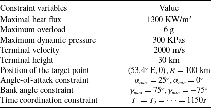
. When the remaining range of the hypersonic vehicle is less than 100 km, the hypersonic vehicle enters the terminal guidance phase and the reentry phase guidance ends. The specific constraint values of the hypersonic vehicle are shown in Table 2. The hardware platform used in the simulation verification process of this article is: CPU: Ryzen 7 8500H with Radeon Graphics; GPU: RTX 3060, the system platform is Windows 11 and the simulation software used is matlab2023b.
Hypersonic vehicle flight constraints

The guidance method designed in this paper is for the cooperative guidance of the reentry phase of the hypersonic vehicles. Therefore, the terminal height is set to 30 km, the distance from the target point is set to 100 km, and the remaining flight phase is the descent attack phase. The terminal height and the radius from the target are set to ensure that the vehicles have the same initial conditions after entering the descent phase, so as to carry out the cooperative guidance of the descent phase.
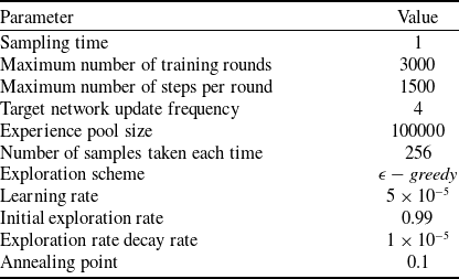
The network parameter settings are shown in Table 3.
Double-DQN network parameters

4.1 Multi-hypersonic vehicles cooperative guidance under no-fly zone constraint
The initial state of the hypersonic vehicle is consistent with that without the no-fly zone constraint, and the parameters of the no-fly zone are shown in Table 4. With the implementation of no-fly zone constraints, the vehicles must continuously assess their distance relative to the no-fly zone during the flight. In order to accomplish the flight mission, it is essential to consider the impact of no-fly zone constraints when approaching the vicinity of the no-fly zone. Once the vehicles move away from the no-fly zone, the primary objective shifts towards achieving the time-coordinated objectives. Therefore, this paper introduces a concept of a ‘warning zone’. When vehicles enter the warning zone, the no-fly zone’s influence on the reward function, donated as
 $ {R}_{2}({s}_{tf})$
, comes into play, guiding the multi-hypersonic vehicles to navigate through the no-fly zone. Once the vehicles exit the warning zone, only
 $ {R}_{1}({s}_{tf})$
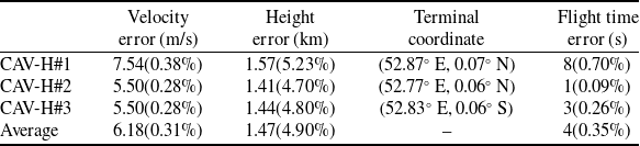
remains in effect, guiding multi-hypersonic vehicles to achieve time coordination. The simulation results are shown in Figs. 5 and 6, and Table 5.
No-fly zone constraint parameters setting

Training reward curve under no-fly zone.

Time co-simulation results of multi-hypersonic vehicles under no-fly zone.

The training reward curve is shown in Fig. 5, where the blue curve represents the reward value for a single training session, and the red curve represents the average reward value for the previous 200 training sessions, from which it can be seen that under the no-fly zone constraints, due to the introduction of the remaining time-of-flight and the absolute value of the bank angle predicted by the predictor-corrector algorithm, the reward value can be maintained at the maximum value of the reward around 200 times of training, and the average reward curve converges at 1000 times of training. Compared with using reinforcement learning alone to achieve time coordination among multiple hypersonic vehicles, the algorithm proposed in this paper incorporates no-fly zone constraints and still achieves a reduction in training iterations by two orders of magnitude. This highlights the superior efficiency of the proposed method in significantly reducing training requirements and improving training performance [Reference Zhang, Yu, Li and Chen28]. The curves in Fig. 6a shows that the heat flow, overload, and dynamic pressure meet the specified constraints. This ensures that the vehicle does not sustain any mechanical or structural damage during reentry. It can be seen from the figure that it can meet the constraints set above. So as to ensure that the vehicle will not produce mechanical or structural damage. The trajectory curves depicted in Figs. 6b and 6c demonstrate the algorithm’s effectiveness in steering multiple hypersonic vehicles towards their designated targets while simultaneously avoiding no-fly zones, as necessitated by the constraints of these restricted areas. The change curve of the bank angle during the flight is shown in 6e. The time coordination and the penetration of the no-fly zone are realised by the change of the bank angle. Because the closer to the target point, the change of the line-of-sight angle is more intense, so the change frequency of the bank angle is also increased. The curve in Fig. 6f represents the designed angle-of-attack planing surface, the terminal altitude of the hypersonic vehicle is related to the angle-of-attack and the bank angle, through the design of the angle-of-attack plane, the terminal altitude of the hypersonic vehicle can be kept within a certain range. Therefore, by designing the angle-of-attack planing surface, the terminal height constraint in the flight mission can be satisfied. The information presented in Table 5 demonstrates that the algorithm successfully enables time-coordinated guidance for multiple hypersonic vehicles within these restricted areas. This evidences the generalisation ability of the proposed algorithm.
Terminal state and error of multi-hypersonic vehicles

4.2 Multi-hypersonic vehicles cooperative guidance under different no-fly zone constraint
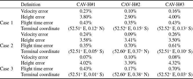
In order to verify the universality of the designed method, and its performance under unseen conditions, the distribution of the no-fly zone is modified after training on the scenario described in 4.1, and the simulation verification is carried out. The simulation results are shown in Fig. 7 and Table 6.
Time co-simulation results of multi-hypersonic vehicles under different no-fly zones.

Terminal state and error of multi-hypersonic vehicles under different no-fly zones

The penetration performance of multi-hypersonic vehicles under three different no-fly zone distributions is shown in Fig. 7. The data in Table 6 show the performance of the designed algorithm under different no-fly zone distributions. It can be seen from the figure that when the distribution of the no-fly zone changes, the designed algorithm can successfully realise the time-coordinated penetration task of different no-fly zones after one training. Compared with Ref. (Reference Zhuang, Li and Wang23), it shows that the algorithm designed in this paper has better universality.
5.0 Conclusion
In this paper, a time-cooperative guidance method based on reinforcement learning for hypersonic vehicles under no-fly zone and other multi-constraint conditions is designed. In order to solve the problems of long training times and limited applicability in reinforcement learning time cooperative guidance, the predictor-corrector method is introduced to estimate the remaining time-of-flight and calculate the absolute value of the bank angle, which are then used as the observations of the reinforcement learning agent. By introducing the predictor-corrector method, the complex decision-making behaviour of the agent is simplified, requiring only the judgement of the bank angle sign at each time step, which significantly improves the training efficiency and reduces the number of training iterations. At the same time, reward function and action space are specifically designed for the tasks of no-fly zone penetration and time coordination, followed by mathematical simulations. Simulations under multiple constraint conditions and different no-fly zone distributions concluded that the proposed algorithm had good applicability, adaptability and robustness in completing the time cooperative no-fly zone penetration task. In the face of increasingly complex flight environments in the future, the operational space for aircraft will become further constrained. Therefore, incorporating dynamic no-fly zones or interceptors in future research would further enhance the applicability and robustness of the proposed algorithm.
Acknowledgements
This work was supported in part by the Key Laboratory of Spacecraft Design Optimization and Dynamic Simulation Technologies, Ministry of Education, in part by the Science and Technology on Complex System Control and Intelligent Agent Cooperation Laboratory, Beijing, 100074, China.