2.1 Dataset

The study uses a comprehensive onboard FDR dataset from a commercial airline. All variables used in this study have a temporal resolution of 1 s. The dataset covers domestic flights within European airspace across 30 route pairs, including flights from August and January to represent typical summer and winter operating conditions. Most flights are short- to medium-haul operations, with durations ranging from approximately one to several hours.

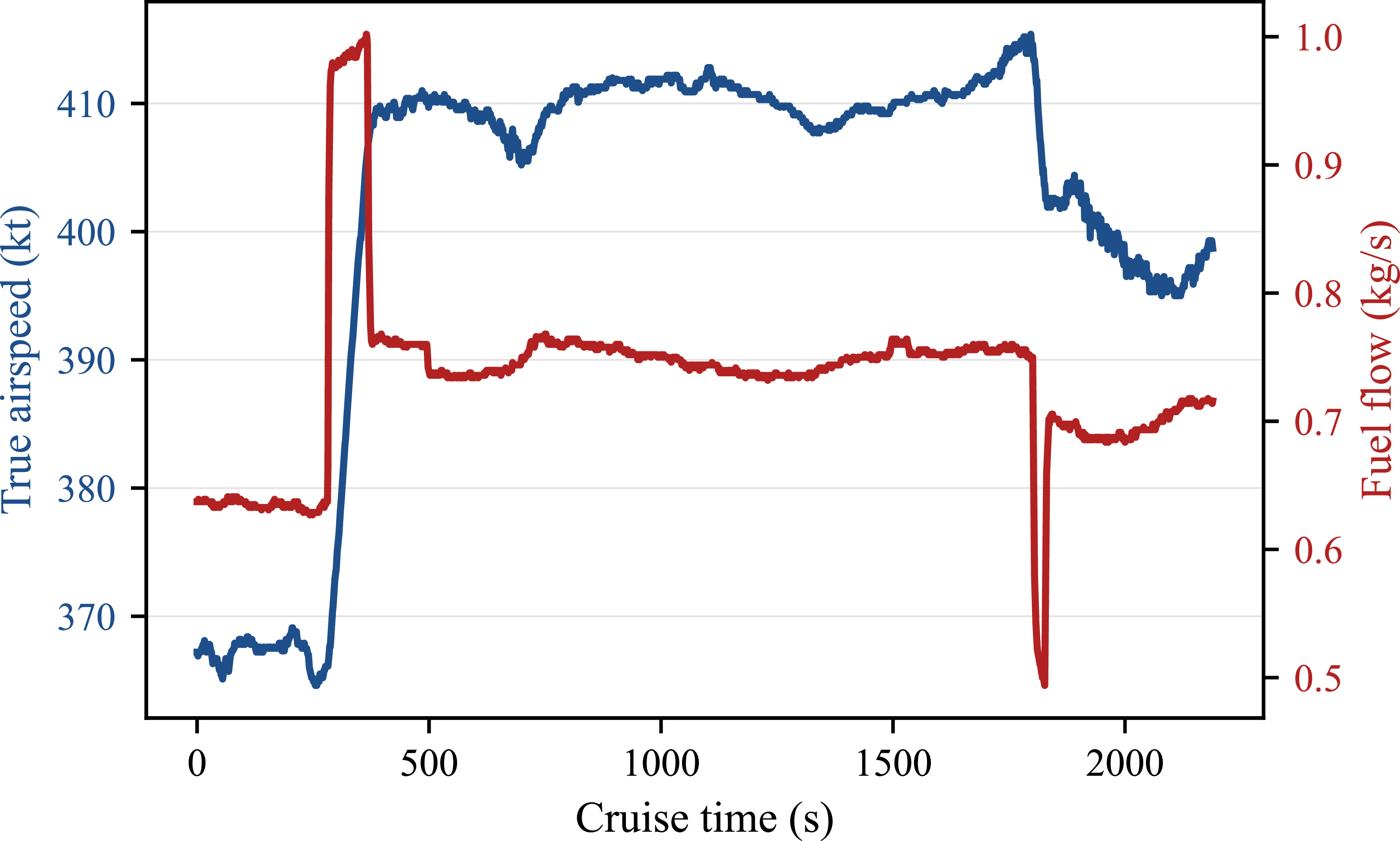
Fuel flow rate during cruise responds to the thrust changes required for acceleration or deceleration during speed adjustments. Figure 1 illustrates the corresponding variations in TAS and fuel flow rate over time. The fuel flow rate increases approximately from 0.63 kg/s to 1.00 kg/s as the aircraft accelerates from 370 kt to 410 kt between 280 and 380 s. Afterward, the fuel flow rate decreases to around 0.75 kg/s. Another remarkable speed change occurs between 1800 and 1840s. During this interval, the airspeed decreases from approximately 410 kt to 403 kt, with a corresponding reduction in fuel flow rate from about 0.75 kg/s to 0.70 kg/s.

Figure 1.

Observed variation in true airspeed (TAS) and fuel flow rate during a representative cruise segment at a pressure altitude of 32,000 ft.

Cruise speeds generally remain relatively stable unless speed changes are required by air traffic constraints, meteorological conditions or airline operating procedures. Nevertheless, as shown in Figure 1, small short-term fluctuations may still occur due to measurement noise and environmental disturbances [Reference Huang, Xu and Johnson9]. Therefore, before filtering the speed variations from the data, it is necessary to set a tolerance value to account for measurement noise and environmental disturbances. This approach is commonly adopted in related research [Reference Lutz, Chatterji and Idris18, Reference Wüstenbecker, Renkhoff, Zeppenfeld, Jameel and Schier-Morgenthal19]. In this study, speed changes of 10 kt or greater are considered. The speed variations should be monitored throughout each flight to exclude small speed changes and to detect flights with speed changes greater than or equal to this tolerance value. To accomplish this, an algorithm was developed to read FDR data stored in 9,879 Excel files, each containing data for a single flight.

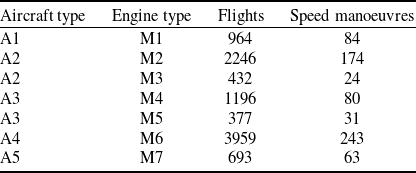
The dataset used in the study comprises five different narrow-bodied twin-engined aircraft, which are frequently used in commercial flights, and seven different engines. Table 1 shows the number of flights for each aircraft and engine type, including the number of speed manoeuvres performed during cruise flight. The aircraft and engine types are anonymised (A1–A5 and M1–M7) due to confidentiality requirements, and this has no impact on the analysis, as the results are independent of specific model names.

Table 1.

Number of flights and speed manoeuvres by aircraft and engine type

Table 1. Long description

A table with five rows and four columns. The columns are labeled Aircraft type, Engine type, Flights, and Speed manoeuvres. The rows present data for different aircraft and engine types. Row 1: Aircraft type A1, Engine type M1, Flights 964, Speed manoeuvres 84. Row 2: Aircraft type A2, Engine type M2, Flights 2246, Speed manoeuvres 174. Row 3: Aircraft type A2, Engine type M3, Flights 432, Speed manoeuvres 24. Row 4: Aircraft type A3, Engine type M4, Flights 1196, Speed manoeuvres 80. Row 5: Aircraft type A3, Engine type M5, Flights 377, Speed manoeuvres 31. Row 6: Aircraft type A4, Engine type M6, Flights 3959, Speed manoeuvres 243. Row 7: Aircraft type A5, Engine type M7, Flights 693, Speed manoeuvres 63.

Fuel flow rates and emissions are calculated using the selected flights, which involve speed manoeuvres.

2.2 Data-processing and manoeuvre-detection

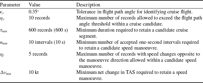
The manoeuvre-extraction procedure consists of two stages: cruise-segment detection followed by speed-manoeuvre detection. The parameter values used in both stages are summarised in Table 2. These parameters were applied consistently to all FDR files before extracting the final manoeuvre dataset. The FDR data, sampled at 1 Hz, were scanned sequentially.

Table 2.

Parameters used in the cruise-segment and speed-manoeuvre detection procedures

Table 2. Long description

The table has three columns: Parameter, Value, and Description. It contains seven rows detailing specific parameters used in the detection procedures. Row 1: Parameter, Flight-path-angle tolerance for identifying near-level flight; Value, 0.35 degrees; Description, Flight-path-angle tolerance for identifying near-level flight. Row 2: Parameter, Maximum number of accepted flight-path-angle threshold violations within a cruise candidate; Value, 10 records; Description, Maximum number of accepted flight-path-angle threshold violations within a cruise candidate. Row 3: Parameter, Minimum length for retaining a candidate cruise segment at the 1-Hz sampling rate; Value, 600 records (600 s); Description, Minimum length for retaining a candidate cruise segment at the 1-Hz sampling rate. Row 4: Parameter, Minimum number of accepted one-second intervals for retaining a speed-manoeuvre candidate; Value, 10 intervals (10 s); Description, Minimum number of accepted one-second intervals for retaining a speed-manoeuvre candidate. Row 5: Parameter, Maximum total number of opposing-direction records tolerated within a speed-manoeuvre candidate; Value, 5 records; Description, Maximum total number of opposing-direction records tolerated within a speed-manoeuvre candidate. Row 6: Parameter, Minimum net true-airspeed change for retaining a speed manoeuvre; Value, 10 kt; Description, Minimum net true-airspeed change for retaining a speed manoeuvre.

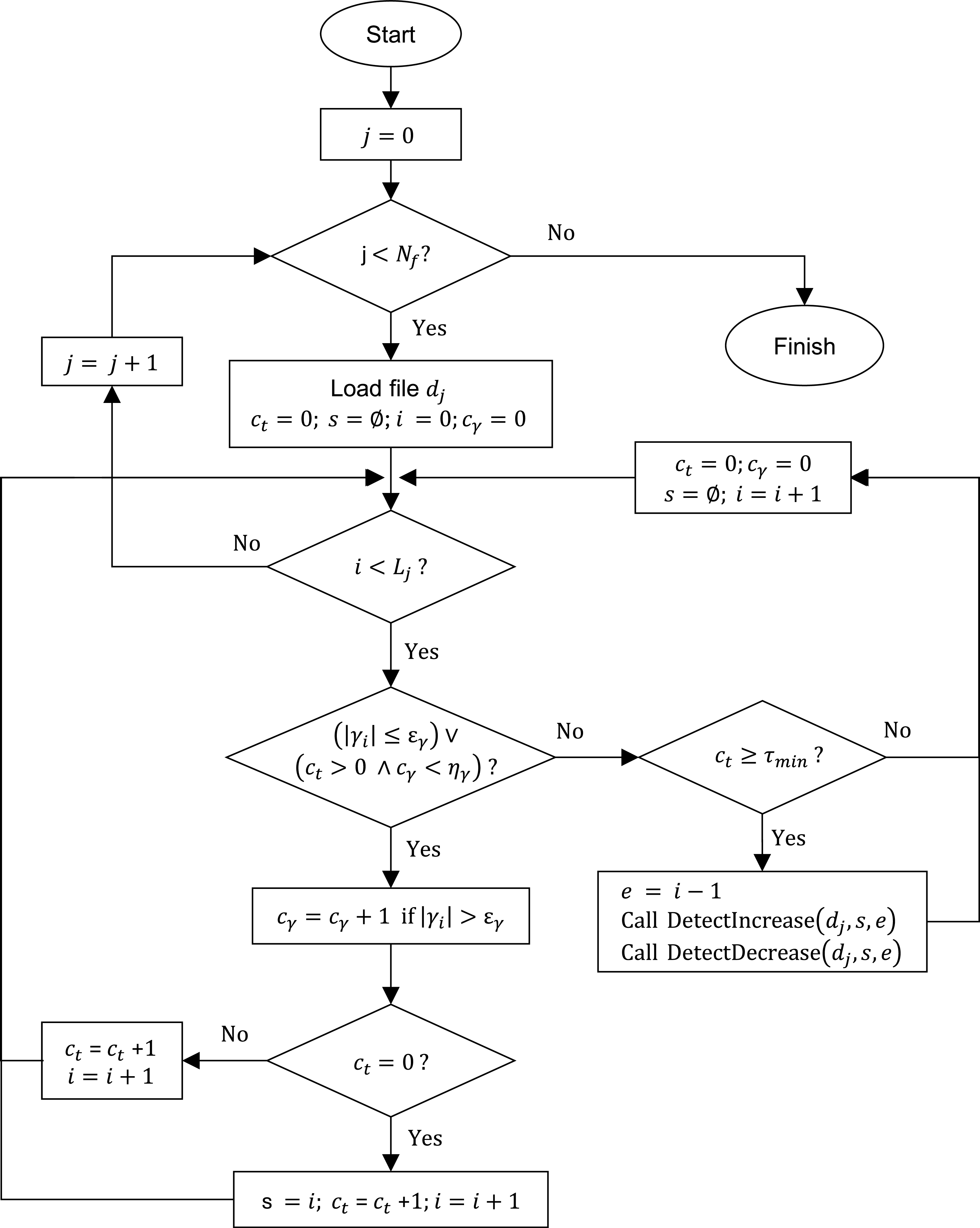
In the first stage, $j$ denotes the file index, $N_f$ is the number of FDR files and $L_j$ is the number of records in file $d_j$ . A cruise candidate began at the first record satisfying the near-level-flight condition, $|\gamma _i|\leq \epsilon _\gamma$ , where $\gamma _i$ is the flight path angle at record $i$ . The counter $c_t$ records the number of accepted 1-s records in the candidate. To prevent brief flight path angle (FPA) fluctuations from fragmenting an otherwise continuous cruise segment, up to $\eta _\gamma$ records exceeding $\epsilon _\gamma$ were permitted after a candidate had begun; $c_\gamma$ records the number of these accepted violations. When neither the near-level-flight condition nor the FPA-violation allowance was satisfied, the preceding record was assigned as the candidate end. Candidates satisfying $c_t\geq \tau _{\min }$ were retained as cruise segments and passed to the second-stage speed-detection procedure. Figure 2 summarises this procedure.

Figure 2.

Flowchart of the cruise-segment detection procedure based on flight path angle tolerance and minimum duration criteria.

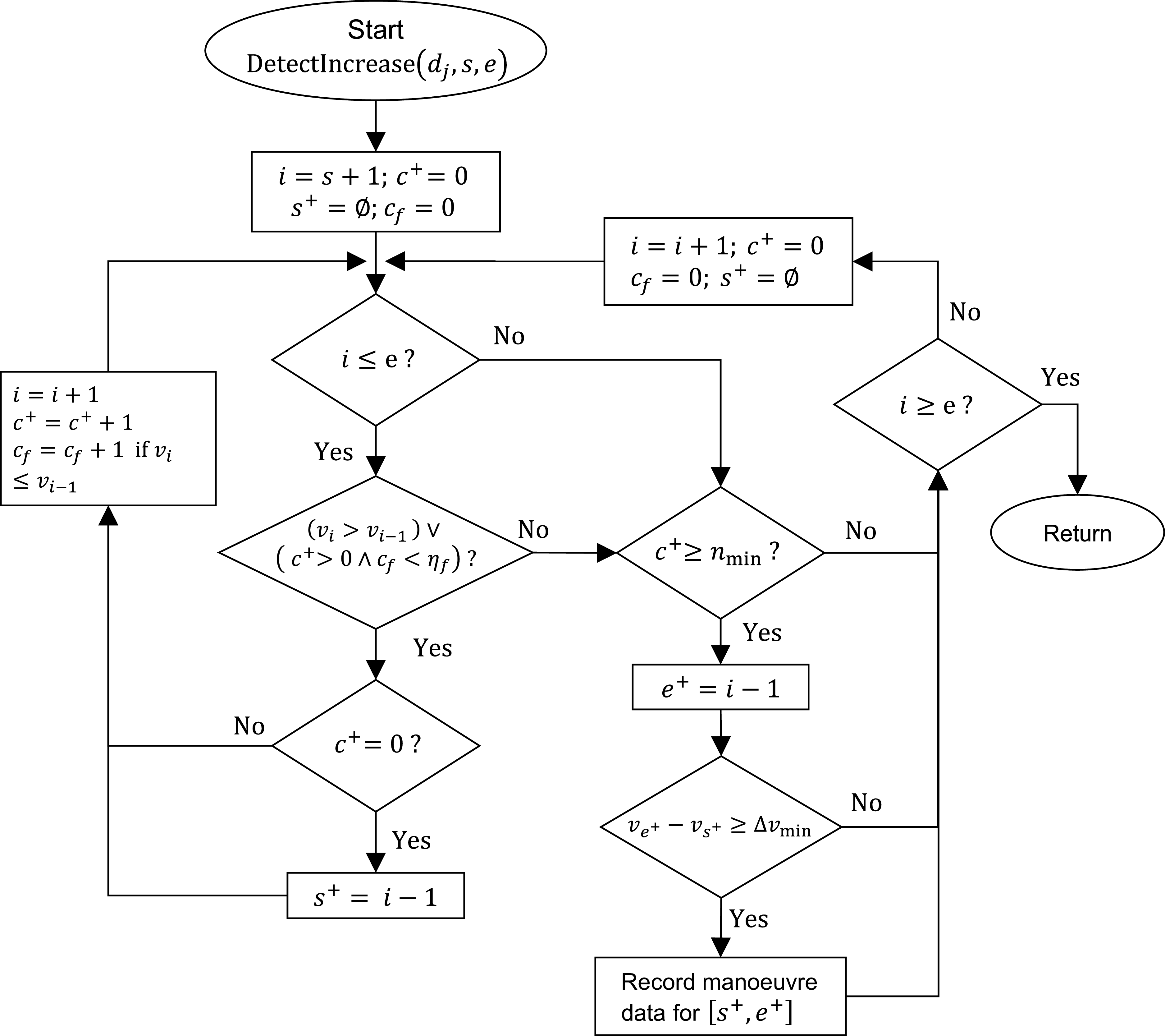
In the second stage, the true-airspeed sequence within each retained cruise interval $[s,e]$ of file $d_j$ was scanned separately for speed increases and decreases. Figure 3 presents the speed-increase procedure. Here, $v_i$ denotes the TAS at record $i$ . Scanning began at $i=s+1$ , and a speed-increase candidate began at $s^+=i-1$ when $v_i\gt v_{i-1}$ . The counter $c^+$ records the number of accepted one-second intervals in the candidate. To prevent short fluctuations from fragmenting an otherwise continuous manoeuvre, a candidate was also continued when $v_i\leq v_{i-1}$ , provided that a candidate was already active and fewer than $\eta _f$ such records had previously been accepted. The counter $c_f$ records the total number of these accepted non-increasing records.

When neither the increasing-speed condition nor the fluctuation allowance was satisfied, the preceding record was assigned as the candidate end, $e^+=i-1$ . The candidate was retained only if it contained at least $n_{\min }$ accepted one-second intervals and its net true-airspeed change satisfied $v_{e^+}-v_{s^+}\geq \Delta v_{\min }$ . The adopted value $\Delta v_{\min }=10$ kt was therefore applied to the difference between the ending and starting TAS of the complete candidate rather than to individual 1-s changes. After a candidate was accepted or rejected, its counters and indices were reset, and scanning continued through the remaining cruise records. Consequently, same-direction variations separated only by the permitted number of non-increasing records remained within one candidate, whereas a longer interruption terminated the candidate and caused the subsequent variation to be evaluated separately.

Speed decreases were detected using the same procedure with the direction inequalities reversed; in that case, $c_f$ counts tolerated non-decreasing records. The corresponding flowchart is not presented to avoid repetition. Candidates were excluded if they occurred outside a retained cruise segment, contained fewer than $n_{\min }$ accepted intervals, did not reach the 10-kt net true-airspeed-change threshold, contained missing or inconsistent FDR records or lacked identifiable start and end indices. Flights without a valid cruise-phase speed manoeuvre remained in the flight dataset but contributed no observations to the manoeuvre analysis. Because aircraft speed may exhibit short-term fluctuations due to measurement noise, sensor uncertainty, turbulence or minor atmospheric disturbances [Reference Huang, Xu and Johnson9], a minimum speed-change threshold was required before a variation was classified as a manoeuvre. Preliminary inspection of the cruise-phase trajectories showed that small fluctuations were typically within an approximately $\pm 5$ kt band. In addition, operational speed adjustments are commonly specified on the order of 0.01–0.04 Mach [Reference Courchelle, Soler, González-Arribas and Delahaye20–Reference Rudnyk, Ellerbroek and Hoekstra22]. In our dataset, the cruise altitudes range from 19,000 ft to 40,000 ft. Under International Standard Atmosphere conditions, 0.01 Mach corresponds approximately to 6.17 kt at 19,000 ft and 5.74 kt at 40,000 ft. Therefore, the adopted 10 kt threshold is more conservative than the lower bound of typical operational speed adjustments expressed in Mach number.

The combined minimum-duration, fluctuation-tolerance and speed-change threshold prevented isolated 1-s spikes and minor cruise-speed variations from being classified as manoeuvres.

Figure 3.

Flowchart of the speed manoeuvre detection procedure illustrated for speed increases within a retained cruise segment.

2.3 Emission calculations

Based on fuel flow data obtained from the FDR, emission indice (EI) at cruise altitudes are calculated for each engine type using the International Civil Aviation Organization (ICAO) Emissions Databank and the Boeing Fuel Flow Method 2 (BFFM2). These methods have been widely employed to estimate aircraft emissions across different phases of flight, ranging from ground operations [Reference Stettler, Koudis, Hu, Majumdar and Ochieng23] to en-route conditions [Reference Chen, Hu, Han, Zhang and Yin24]. The BFFM2, developed by Boeing, enables emission indices defined at sea-level reference conditions to be corrected to any atmospheric conditions [Reference DuBois and Paynter25]. EI is defined as the mass of pollutant emitted per unit mass of fuel burned. Emission indices at flight altitude are calculated for HC, CO and $\mathrm{NO_x}$ using the following equations:

(1) \begin{eqnarray} \mathrm{EI}_{\mathrm{HC}}^{\mathrm{alt}} = \mathrm{EI}_{\mathrm{HC}}^{\mathrm{sl}} \left ( \frac {\theta _{\mathrm{amb}}^{3.3}}{\delta _{\mathrm{amb}}^{1.02}} \right ) \\[-20pt] \nonumber \end{eqnarray}

(2) \begin{eqnarray} \mathrm{EI}_{\mathrm{CO}}^{\mathrm{alt}} = \mathrm{EI}_{\mathrm{CO}}^{\mathrm{sl}} \left ( \frac {\theta _{\mathrm{amb}}^{3.3}}{\delta _{\mathrm{amb}}^{1.02}} \right ) \\[-20pt] \nonumber \end{eqnarray}

(3) \begin{eqnarray} \mathrm{EI}_{\mathrm{NO_x}}^{\mathrm{alt}} = \mathrm{EI}_{\mathrm{NO_x}}^{\mathrm{sl}} \left ( \frac {\delta _{\mathrm{amb}}^{1.02}}{\theta _{\mathrm{amb}}^{3.3}} \right )^{0.5} \mathrm{e}^{H} \\[10pt] \nonumber \end{eqnarray}

where

\begin{eqnarray*} \theta _{\mathrm{amb}} = \frac {T_{\mathrm{amb}}}{T_{\mathrm{sl}}}, \qquad \delta _{\mathrm{amb}} = \frac {P_{\mathrm{amb}}}{P_{\mathrm{sl}}}, \qquad H = -19(\omega - 0.00634). \end{eqnarray*}

Humidity ratio is calculated using the ISO Standard Atmosphere (ISO 5878) as follows. The FDR ambient temperature is used in degrees Celsius to calculate saturation vapour pressure and is converted to kelvin for the BFFM2 temperature ratio and atmospheric-pressure calculations. Relative humidity is expressed as a fraction:

(4) \begin{align} \omega =& \frac {0.62197058 \, \mathrm{RH} \, \times P_{\mathrm{sat}}} {\left ( P_{\mathrm{amb}} \times 68.9476 \right ) - \left ( \mathrm{RH} \, \times P_{\mathrm{sat}} \right )} \\[-10pt] \nonumber \end{align}

(5) \begin{align} &\,\, P_{\mathrm{sat}} = 6.107 \times 10^{\frac {7.5 \, T_{\mathrm{amb,C}}} {237.3 + T_{\mathrm{amb,C}}}} \\[-10pt] \nonumber \end{align}

(6) \begin{align} &\quad T_{\mathrm{amb}} = T_{\mathrm{amb,C}} + 273.15 \\[12pt] \nonumber \end{align}

In Equations (4)–(6), $P_{\mathrm{amb}}$ is expressed in psia, $P_{\mathrm{sat}}$ in hPa, and the factor 68.9476 converts $P_{\mathrm{amb}}$ from psia to hPa. The assumed relative humidity (RH) is entered as $\mathrm{RH}=0.60$ .

Below the tropopause, the ambient pressure is computed as

(7) \begin{eqnarray} P_{\mathrm{amb}} = P_{\mathrm{sl}} \left ( 1 - \frac {\alpha }{T_{\mathrm{sl}}} \, h \right )^{\frac {g_0}{\alpha R}} \end{eqnarray}

Above the tropopause [26],

(8) \begin{eqnarray} P_{\mathrm{amb}} = P_1 \, \mathrm{e}^{\frac {-g_0 (h - h_1)}{R T_1}} \end{eqnarray}

Because the ICAO Databank reports fuel flow rate on a per-engine basis, the total-aircraft fuel flow rate recorded by the FDR is divided by the number of engines before applying the BFFM2 correction:

(9) \begin{equation} W_f^{\mathrm{alt}} = \frac {FF}{N_e}. \end{equation}

The equivalent per-engine sea-level fuel flow rate is then calculated using the Mach number and the ambient absolute temperature obtained after converting the FDR temperature from degrees Celsius to kelvin:

(10) \begin{eqnarray} W_f^{\mathrm{sl}} = W_f^{\mathrm{alt}} \left ( \frac {\theta _{\mathrm{amb}}^{3.8}}{\delta _{\mathrm{amb}}} \right ) \mathrm{e}^{0.2 M^2} \end{eqnarray}

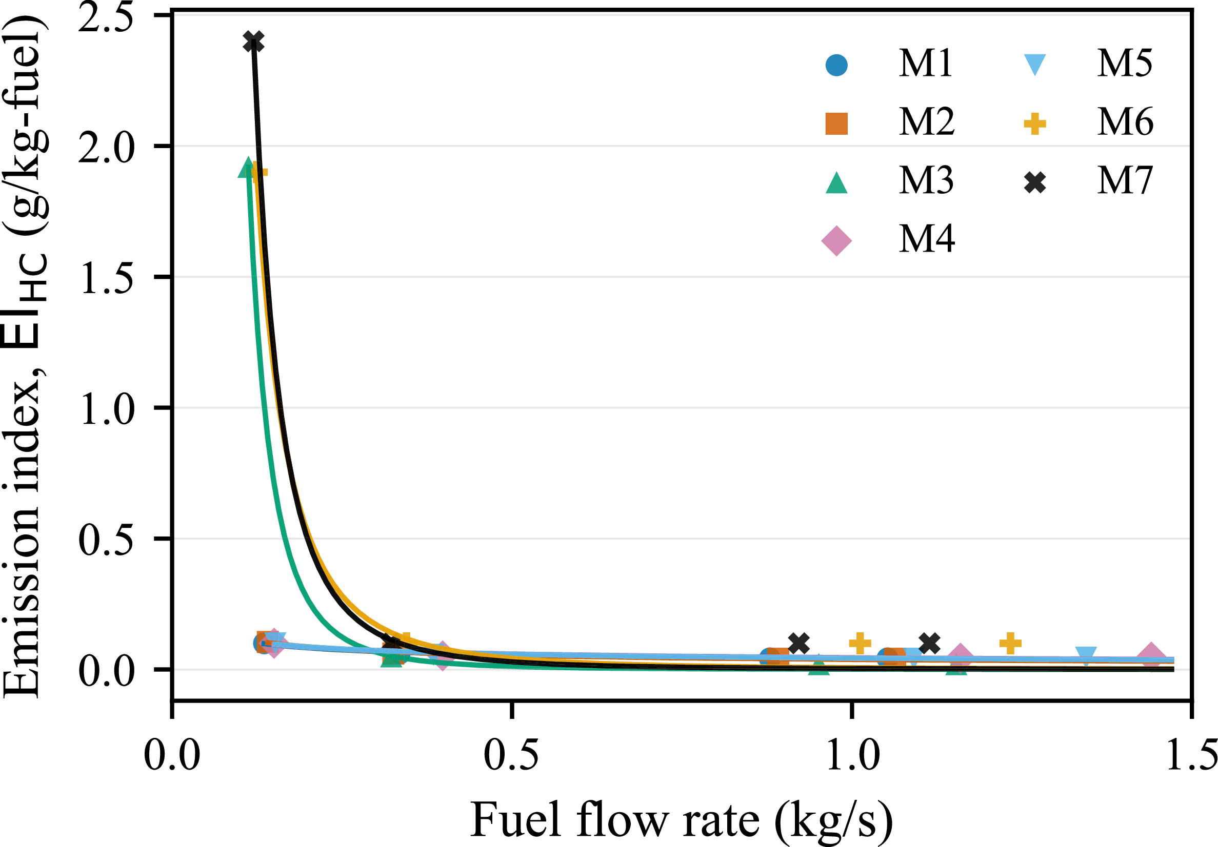
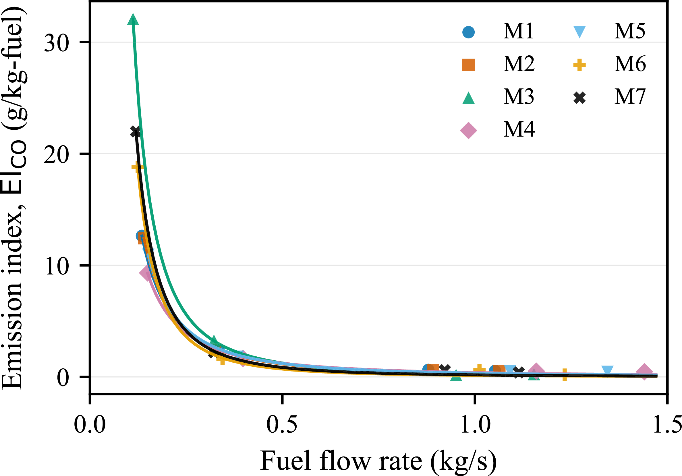
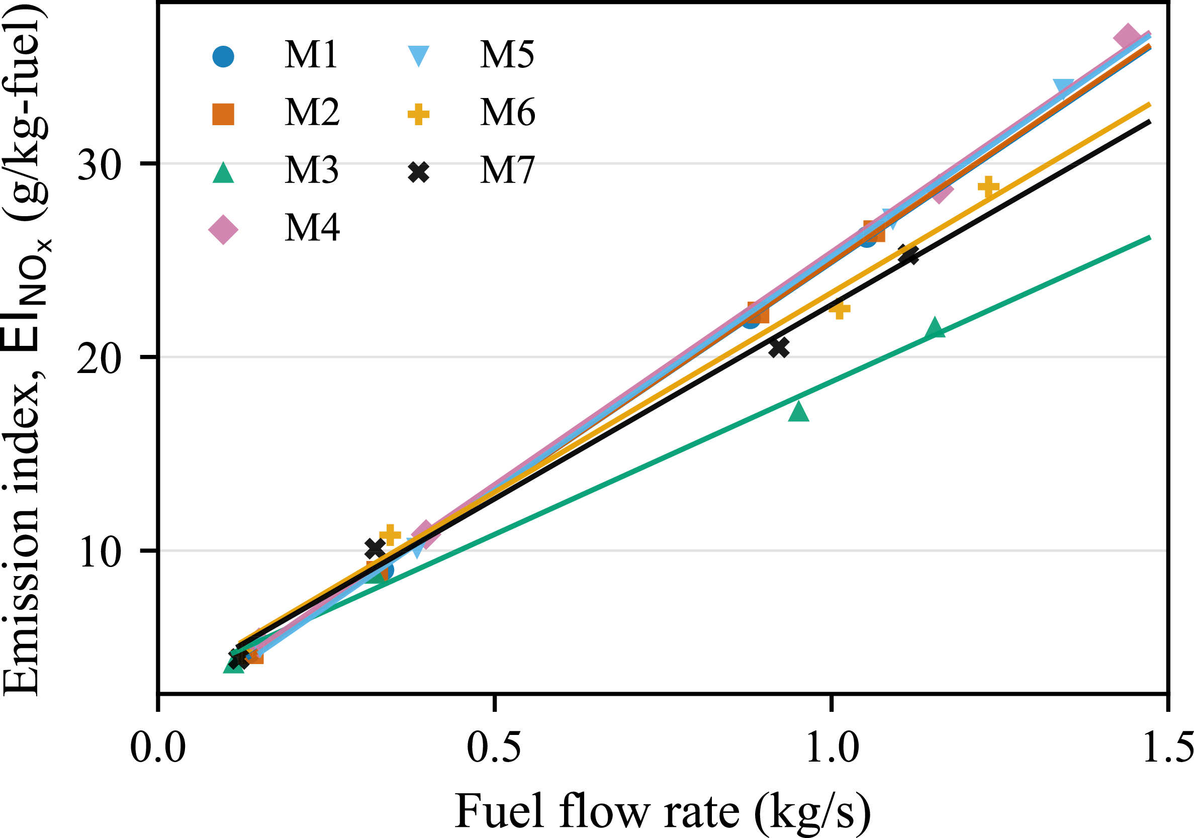
After obtaining the fuel flow rates at sea level, the corresponding sea level emission indices using the calculated fuel flow rates can be obtained using the ICAO emission databank [27]. In this databank, emission indices are provided for four thrust settings (taxi (7%), approach (30%), climb (70%), take-off (100%)) including fuel flow rates (assumed to be constant) for each engine type. However, since aircraft fly with different thrust settings and fuel flow rates, emission indices should be determined for the fuel flow rates not reported in the ICAO emission databank. For this purpose, a curve-fitting method is applied to seven different engine types for each emission index, as shown in Figures 4, 5 and 6.

The emission index for HC and CO tends to decrease exponentially with the increase in the fuel flow rate. Consequently, an exponentially descending curve was created for each engine type for both HC and CO emission indices, and the $\mathrm{R}^2$ values were greater than 0.99 and 0.88, respectively. There is a linear relationship between $\mathrm{NO_x}$ emission index and fuel flow rate. Hence, a linear model was created for each engine type, with the $\mathrm{R}^2$ values greater than 0.99.

Figure 4.

Curve-fitted relationships between equivalent sea-level fuel flow rate and the sea-level HC emission index across engine types.

Figure 5.

Curve-fitted relationships between equivalent sea-level fuel flow rate and the sea-level CO emission index across engine types.

Figure 6.

Linear relationships between equivalent sea-level fuel flow rate and the sea-level $\mathrm{NO_x}$ emission index across engine types.

The cumulative emission mass of pollutant $k$ for a single aircraft can be expressed, following the ICAO formulation [28], as

(11) \begin{eqnarray} E_{k} = t \times FF \times \mathrm{EI}_{k}, \end{eqnarray}

where $t$ denotes the time required for a speed change (s), $FF$ denotes the total-aircraft fuel flow rate for both engines (kg/s), and $\mathrm{EI}_{k}$ denotes the emission index of pollutant $k$ (g/kg-fuel).

2.4 Determination of variables

The fuel flow rate depends on various parameters such as engine/aircraft type, TAS, aircraft mass, atmospheric density, wing reference area, climb/descent rate and flight path angle [Reference Collins29]. However, because this study focuses on speed manoeuvres during the cruise phase, climb/descent rate and flight path angle were not retained as explanatory variables. Atmospheric density mostly depends on flight altitude, and some characteristics such as wing reference area are related to aircraft type. In our dataset, since each aircraft type uses a different engine type, it is sufficient to consider the engine type as a variable covering both engine and aircraft type. Therefore, initially, engine type, aircraft mass during the manoeuvre( $m$ ), TAS during the manoeuvre, flight level ( $FL$ ) and net change in true airspeed ( $\Delta \mathrm{TAS}$ ) are selected as the variables to predict the change in fuel flow rate ( $\Delta FF$ ).

3.1 Characteristics of speed manoeuvres

In the dataset, 239 speed increases and 460 speed decreases satisfy the criterion of a net true-airspeed change of 10 kt or greater. Speed reductions account for 66% of all speed manoeuvres. The analysis presented hereafter is based on this subset of data.

Statistical analyses were first conducted to identify variables relevant to predicting the change in fuel flow rate, ( $\Delta FF$ ) during speed manoeuvres. Pearson correlation analysis was applied to examine the relationships between $\Delta FF$ and the candidate explanatory variables. 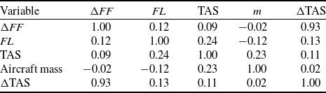As shown in Table 3, $\Delta \mathrm{TAS}$ exhibits a strong positive correlation with $\Delta FF$ ( $r = 0.93$ ), whereas $FL$ , $\mathrm{TAS}$ and aircraft mass during the manoeuvre, show only weak correlations. In addition, no strong correlations are observed among the explanatory variables, indicating the absence of significant collinearity. These results suggest that $\Delta \mathrm{TAS}$ is the dominant factor influencing $\Delta FF$ during the speed manoeuvres.

Table 3.

Pearson correlation coefficients for the speed-manoeuvre variables

Table 3. Long description

A table titled ‘Pearson correlation coefficients for the speed-manoeuvre variables’ with five rows and five columns. The table includes the following variables: delta FF, FL, TAS, m, and delta TAS. Each cell contains a correlation coefficient value. Row 1: delta FF, 1.00, 0.12, 0.09, -0.02, 0.93. Row 2: FL, 0.12, 1.00, 0.24, -0.12, 0.13. Row 3: TAS, 0.09, 0.24, 1.00, 0.23, 0.11. Row 4: m, -0.02, -0.12, 0.23, 1.00, 0.02. Row 5: delta TAS, 0.93, 0.13, 0.11, 0.02, 1.00.

A one-way ANOVA test was conducted to examine whether $\Delta FF$ during speed manoeuvres differ across engine types. The results indicate no statistically significant differences among engine types, with the exception of engine M4. To further investigate whether this observed difference is attributable to engine type or aircraft type, an additional one-way ANOVA was performed using aircraft type as the grouping factor. 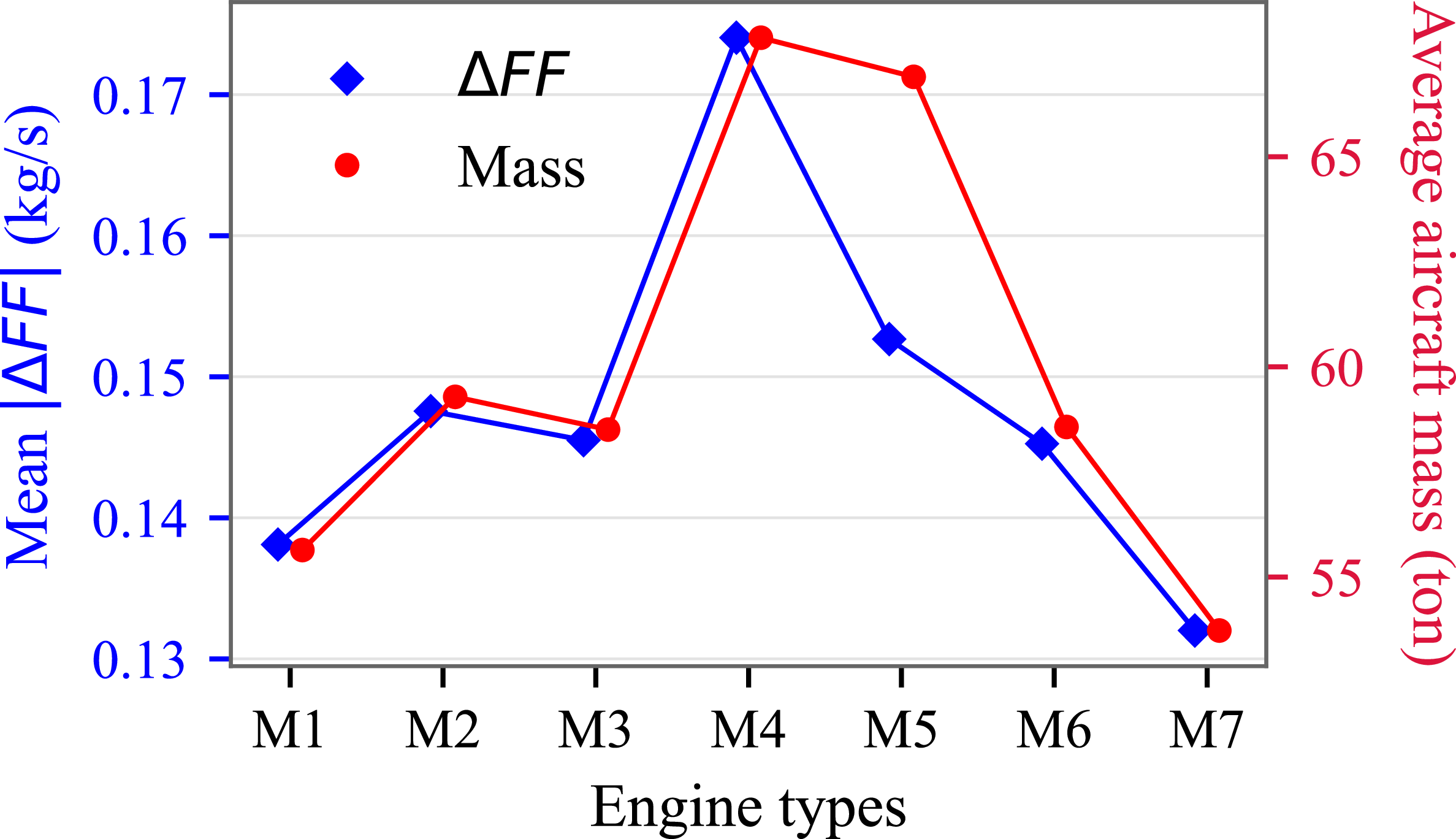In this case, aircraft type A3 was found to differ from the others in terms of $\Delta FF$ during speed manoeuvres. Notably, this aircraft type also exhibits the highest mean mass, suggesting that the observed differences are more likely related to aircraft mass rather than engine or aircraft type alone. The relationship between the mean absolute change in fuel flow rate and the mean aircraft mass for different engine types is illustrated in Figure 7. Since changes in fuel flow rates are negative during speed reductions, absolute values are used for consistency.

Although a relationship between $\Delta FF$ and aircraft mass may be intuitively expected, the observed correlation is weak, as shown in Table 3. When speed increases and speed decreases are considered separately using Pearson correlation analysis, the correlation coefficients are $r = 0.171$ and $r = -0.189$ , respectively, still indicating a very weak association between $\Delta FF$ and aircraft mass. The baseline regression analysis was conducted using $\Delta \mathrm{TAS}$ as the sole predictor.

Figure 7.

Mean absolute fuel flow rate change and mean aircraft mass during speed manoeuvres across engine types.

Figure 8.

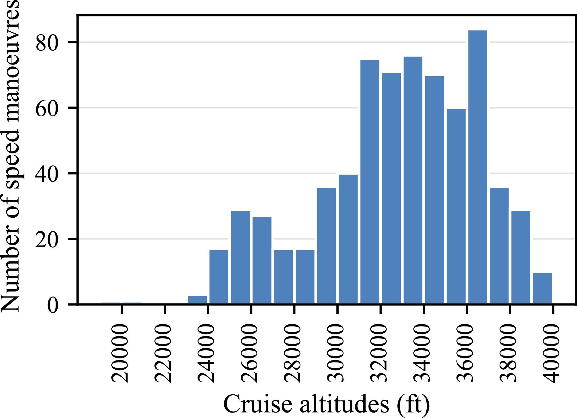
Distribution of detected speed manoeuvres across cruise altitudes.

The frequency of speed manoeuvres according to flight altitude is illustrated in Figure 8. The speed manoeuvres are mostly performed at 36,000 ft, while no speed manoeuvres are executed below 19,000 ft or above 40,000 ft. The frequencies are concentrated between 29,000 ft and 38,000 ft.

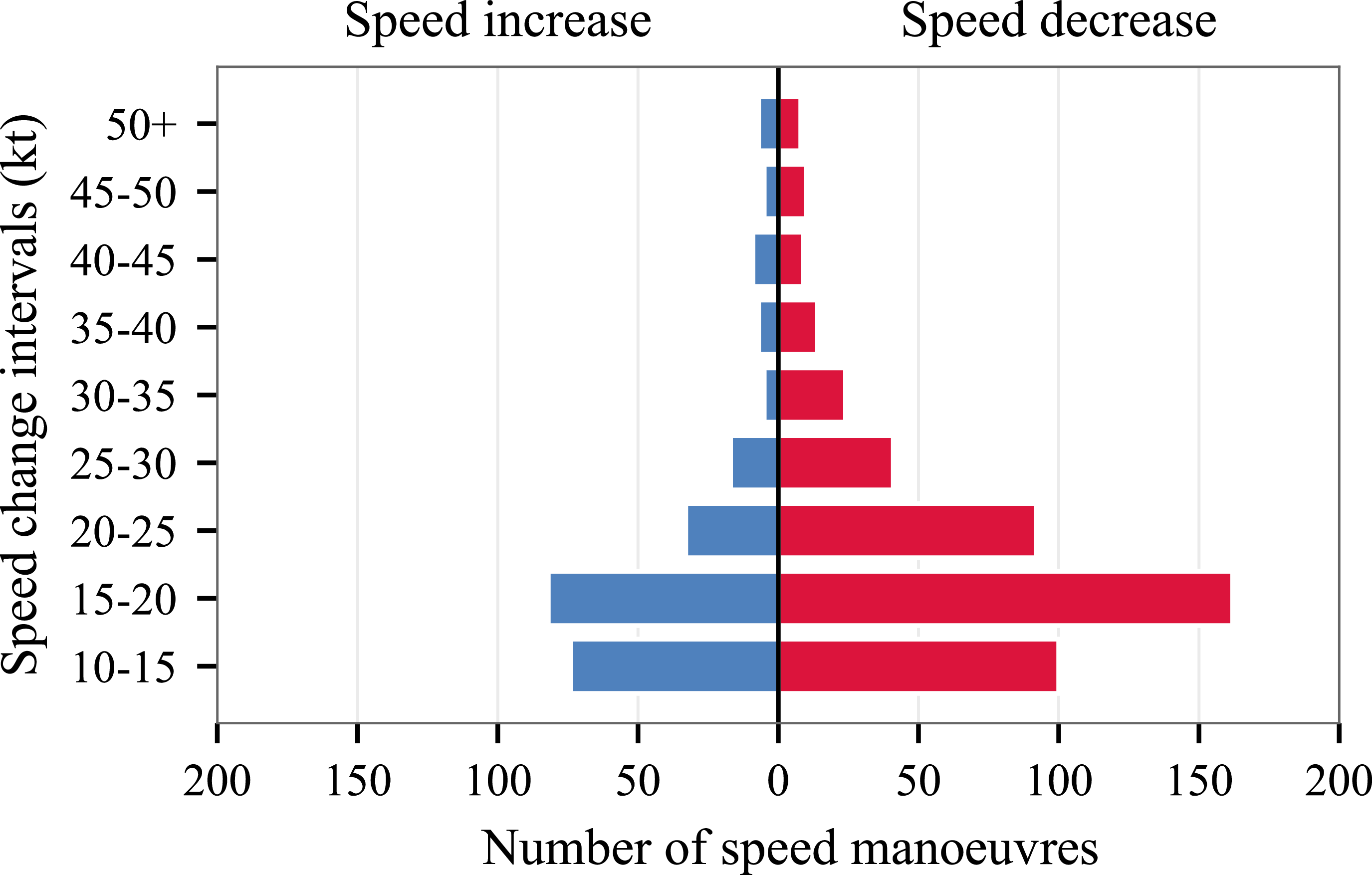
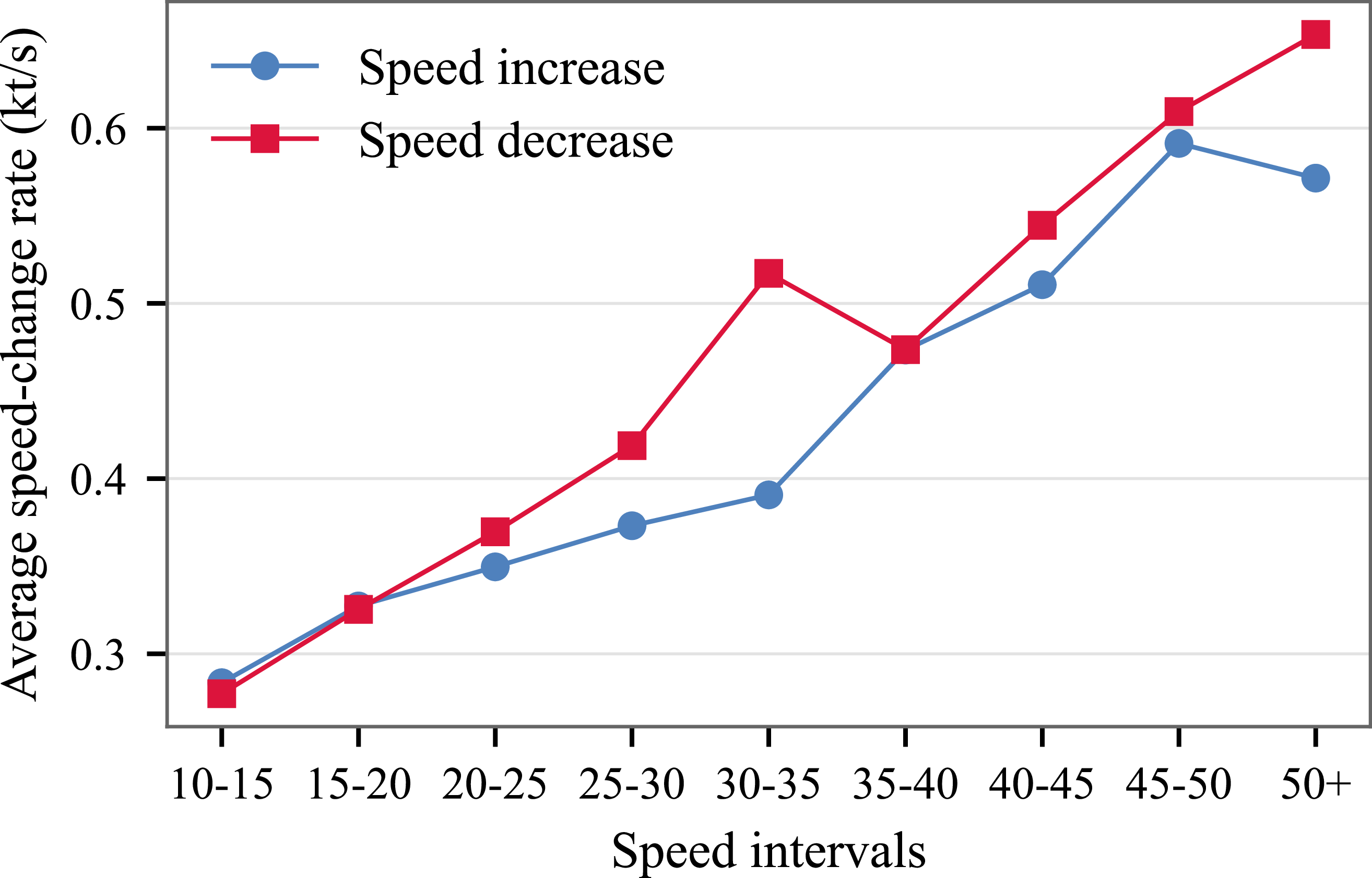
The speed changes are grouped from 10 to 50 kt into 5-kt intervals. As shown in Figure 9, the speed manoeuvres are performed mostly between 10 and 20 kt for speed increases, and between 10 and 25 kt for speed decreases.

Figure 9.

Distribution of speed-increase and speed-decrease manoeuvres across net true airspeed change intervals.

Figure 10.

Average speed change rates for speed increase and speed decrease manoeuvres across net true airspeed change intervals.

The average speed-change rate for increases and decreases is shown in Figure 10. On average, speed increases occur at 0.35 kt/s (standard deviation = 0.09 kt/s), whereas speed decreases occur at 0.36 kt/s (standard deviation = 0.11 kt/s), indicating that speed increases are, on average, slightly less aggressive than speed decreases. At small speed variations, the influence of measurement noise becomes more noticeable, resulting in larger relative fluctuations. Conversely, at higher magnitudes of speed change, reductions are executed faster than increases. For instance, using 20 kt as a tolerance threshold, speed decreases occur approximately 5% faster than increases, compared to an overall difference of 3.2%. Furthermore, larger speed changes are performed at a higher rate; for example, when the change exceeds 20 kt, speed decreases and increases are executed 28.7% and 23.8% faster, respectively, than for changes below 20 kt.

Our analysis shows that during speed increases, the fuel flow rate and the $\mathrm{NO_x}$ emission index rise by 25% and 22%, respectively, whereas during speed decreases, they drop by 23% and 22%. It can be noted that the rates of the changes in the fuel flow rate and $\mathrm{NO_x}$ emission index are quite similar during a speed manoeuvre. On the other hand, HC and CO emission indices decrease by 12% and 34% during speed increases, and they increase by 20% and 76% during speed decreases.

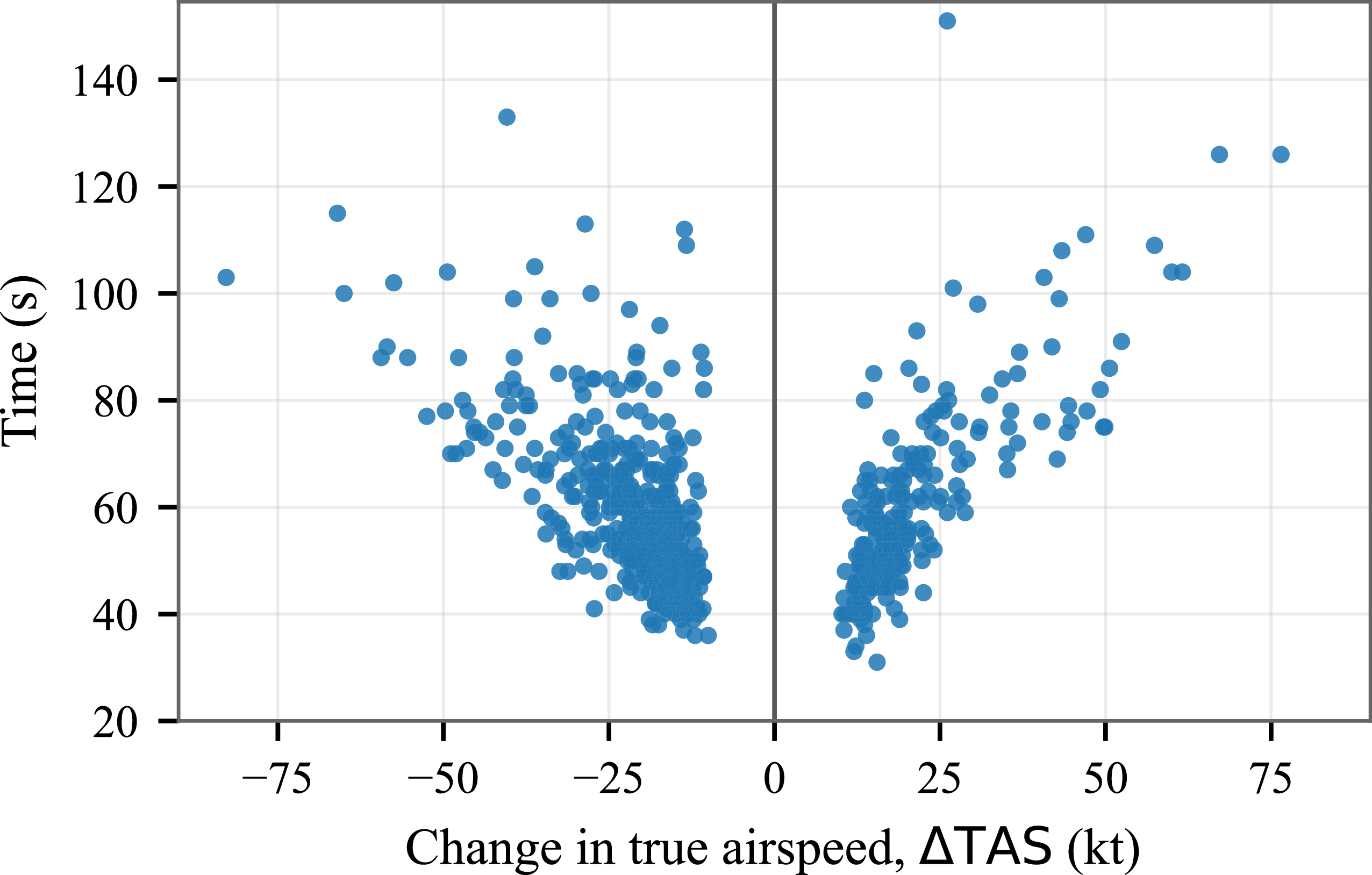
The durations of speed manoeuvres involving speed changes of 10 kt or greater are presented in the scatterplot in Figure 11. It can be noted that there is a close linear relationship between the amount of speed change and the time that is required to complete a speed change. Although the $\mathrm{R}^2$ value of the relationship is not high (the $\mathrm{R}^2$ value is found to be 0.61 for the speed increase, 0.40 for speed decrease) due to differences such as the rate of speed and meteorological conditions’ still, a general trend shows that higher speed changes take longer.

Figure 11.

Relationship between net true-airspeed change and manoeuvre duration.

3.2 Speed change impacts on fuel flow rate and emissions

To quantify the effect of speed changes on fuel flow rate and emissions during speed manoeuvres, regression analyses were conducted between the magnitude of TAS change and the corresponding average changes in fuel flow rate and emission indices over each manoeuvre.

Figure 12.

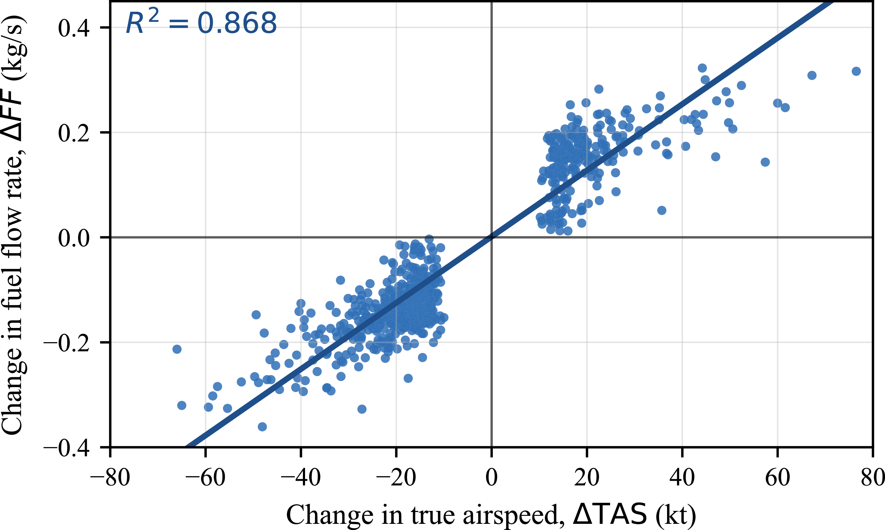
Linear relationship between true airspeed change and fuel flow rate change.

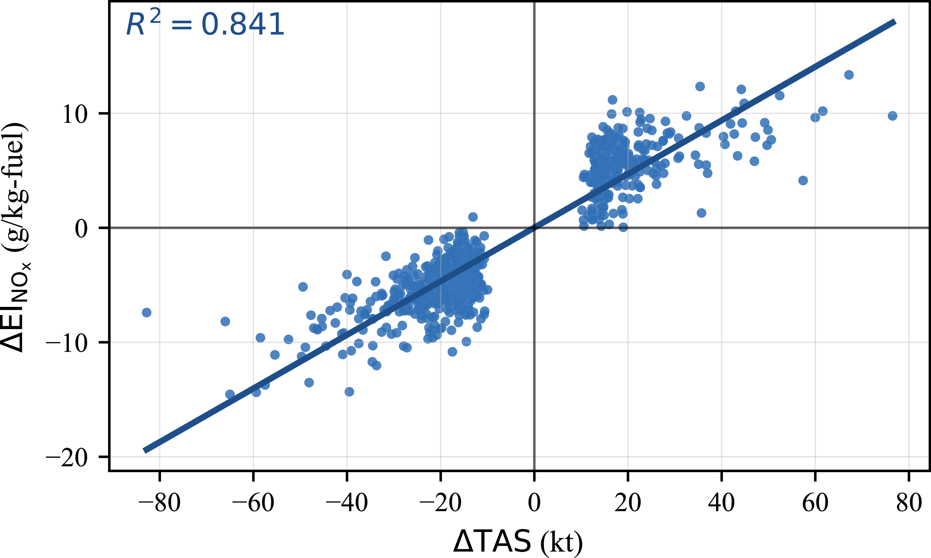
Figures 12 and 13 show strong linear relationships between true airspeed change and the corresponding variations in fuel flow rate and $\mathrm{NO_x}$ emission index, respectively. The regression models explain 86.8% and 84.1% of the observed variability for fuel flow rate and $\mathrm{NO_x}$ emissions, respectively ( $p \lt 0.001$ ). These models indicate proportional responses of fuel flow rate and $\mathrm{NO_x}$ emissions to changes in true airspeed, as described by Equations (12) and (13).

(12) \begin{align} \Delta FF = 6.31\times 10^{-3}\,\Delta \mathrm{TAS} + 1.40\times 10^{-3}, \\[-9pt] \nonumber \end{align}

(13) \begin{align} \Delta \mathrm{EI}_{\mathrm{NO_x}} = 2.34\times 10^{-1}\,\Delta \mathrm{TAS} + 1.64\times 10^{-2}, \\[10pt] \nonumber \end{align}

Figure 13.

Linear relationship between true airspeed change and $\mathrm{NO_x}$ emission index change.

Figure 14.

Quadratic relationship between true airspeed change and HC emission index change.

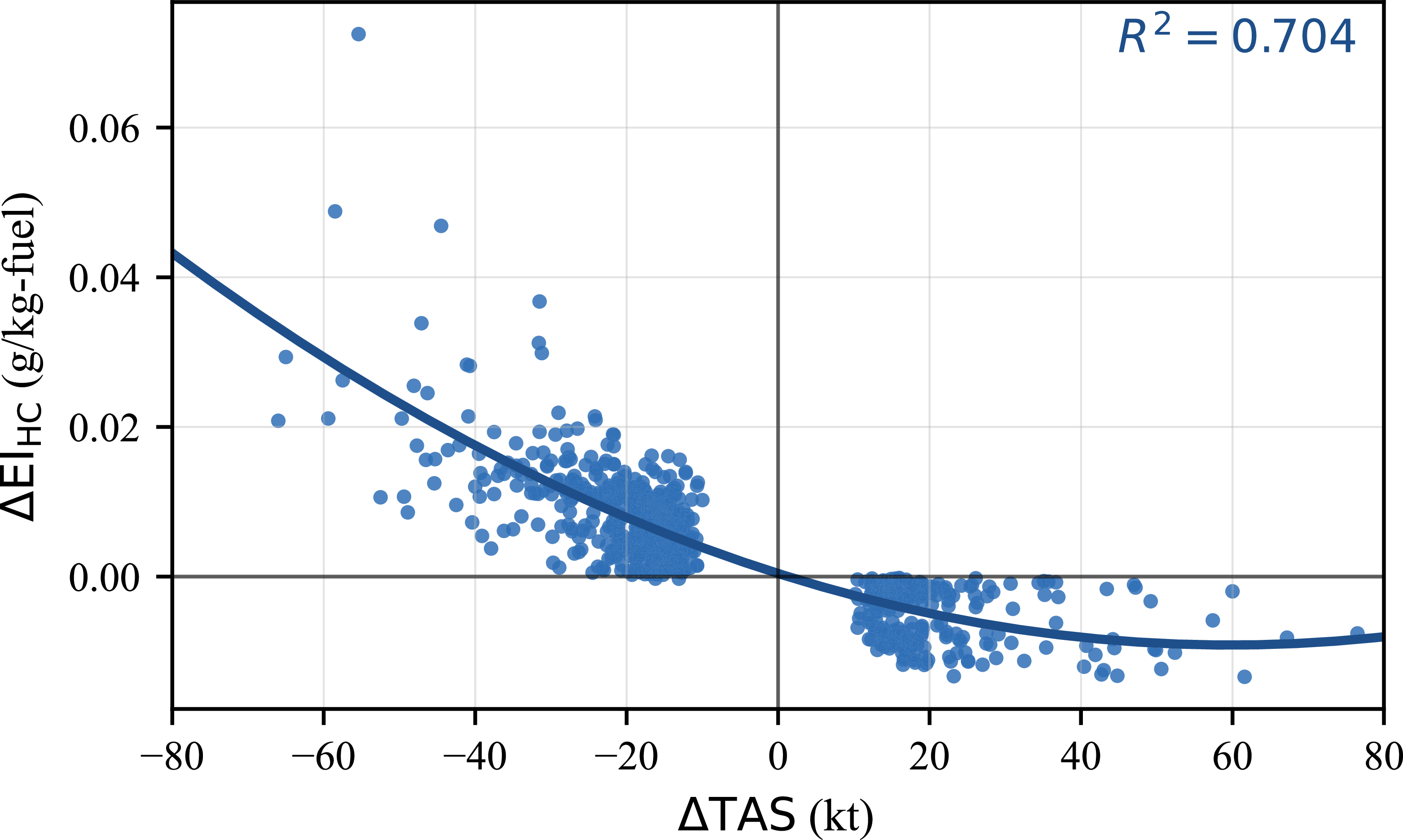
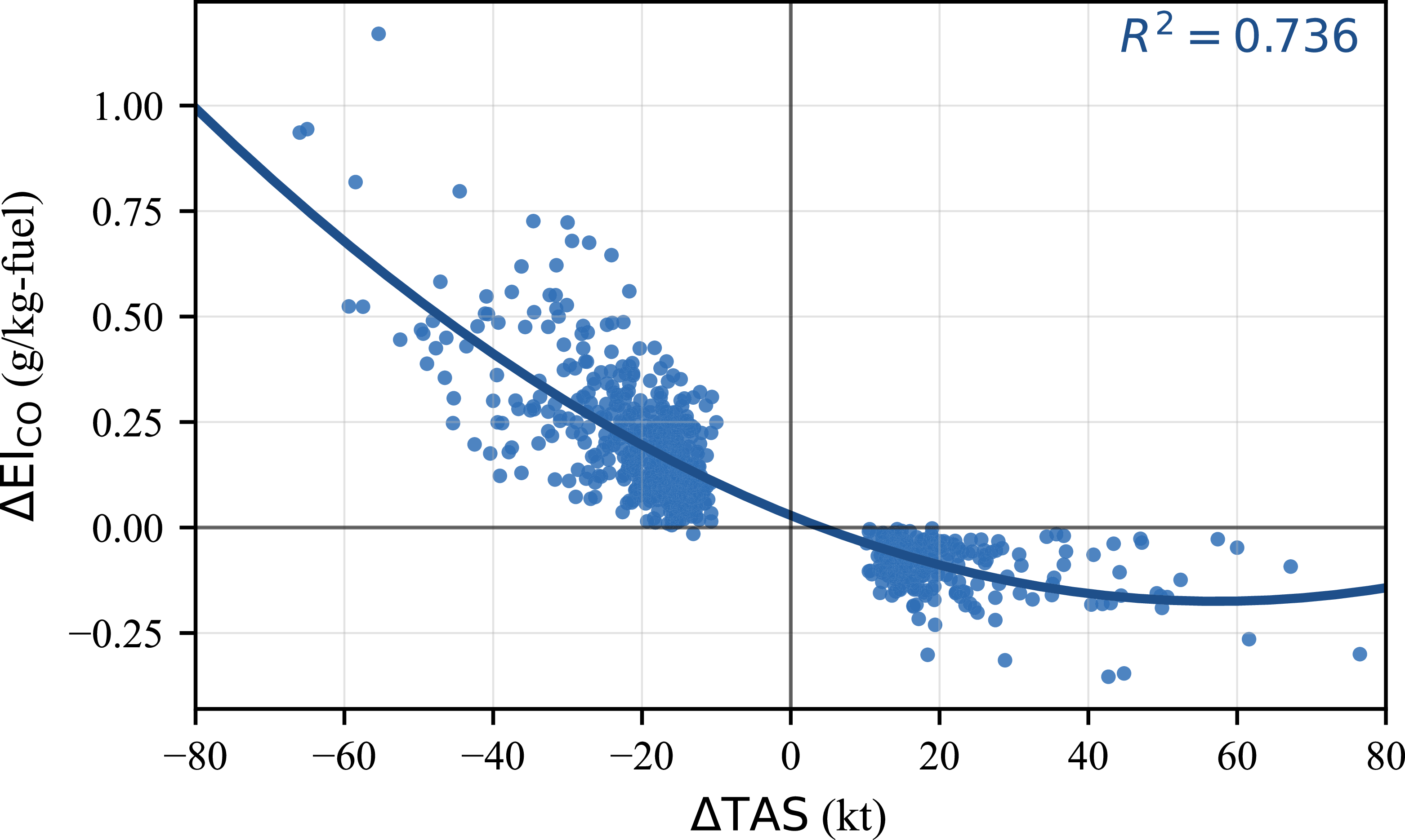
In contrast to fuel flow rate and $\mathrm{NO_x}$ emissions, the responses of HC and CO emission indices to speed changes are better represented by quadratic models as shown in Figures 14 and 15. The corresponding regressions explain 70.4% and 73.6% of the observed variability for HC and CO, respectively ( $p \lt 0.001$ ). The presence of both linear and quadratic terms indicates nonlinear and asymmetric responses of HC and CO emissions to acceleration and deceleration during speed manoeuvres, as described by Equations (14) and (15).

(14) \begin{align} \Delta \mathrm{EI}_{\mathrm{HC}} = 2.68\times 10^{-6}\,(\Delta \mathrm{TAS})^2 - 3.20\times 10^{-4}\,\Delta \mathrm{TAS} + 4.20\times 10^{-4}, \\[-8pt] \nonumber \end{align}

(15) \begin{align} \Delta \mathrm{EI}_{\mathrm{CO}} = 6.20\times 10^{-5}\,(\Delta \mathrm{TAS})^2 - 7.10\times 10^{-3}\,\Delta \mathrm{TAS} + 2.85\times 10^{-2}, \\[11pt] \nonumber \end{align}

It should be noted that the absolute magnitudes of HC and CO emissions are considerably smaller than those of $\mathrm{NO_x}$ , as these emissions are primarily associated with low-thrust operating conditions.

The distinction between the linear and quadratic regression forms can be understood from the sequence of relationships used in the emission calculations. Speed change produces an approximately linear change in fuel flow rate, whereas HC and CO emission indices vary nonlinearly with fuel flow rate. Since HC and CO are products of incomplete combustion, their emission indices are sensitive to changes in combustion efficiency.

3.3 Statistical validation and robustness assessment

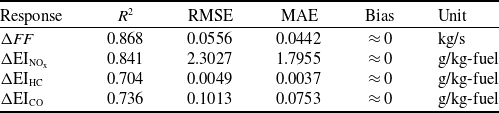
In addition to the coefficient of determination, the regression models were evaluated using the root mean square error (RMSE), mean absolute error (MAE), and mean bias. Bias was calculated as the mean prediction error, defined as the predicted value minus the observed value. These metrics provide complementary information on the magnitude and direction of the model errors. The resulting in-sample performance metrics are summarised in Table 4.

Table 4.

In-sample performance metrics of the regression models

Table 4. Long description

A table with five rows and five columns. The columns are labeled Response, R squared, RMSE, MAE, Bias, and Unit. The rows are labeled with different responses: delta FF, delta EI NO_x, delta EI HC, and delta EI CO. Each row provides values for R squared, RMSE, MAE, Bias, and Unit. The units for the responses are kg/s and g/kg-fuel. The table presents the in-sample performance metrics of the regression models, including the coefficient of determination, root mean square error, mean absolute error, and mean bias.

Figure 15.

Quadratic relationship between true airspeed change and CO emission index change.

The $\Delta FF$ and $\Delta \mathrm{EI}_{\mathrm{NO_x}}$ models showed the strongest in-sample performance, with $R^2$ values of 0.868 and 0.841, respectively. The corresponding MAE values were 0.0442 kg/s for $\Delta FF$ and 1.7955 g/kg-fuel for $\Delta \mathrm{EI}_{\mathrm{NO_x}}$ . The $\Delta \mathrm{EI}_{\mathrm{HC}}$ and $\Delta \mathrm{EI}_{\mathrm{CO}}$ models showed more moderate explanatory performance, with $R^2$ values of 0.704 and 0.736, respectively. The mean bias values were close to zero for all models.

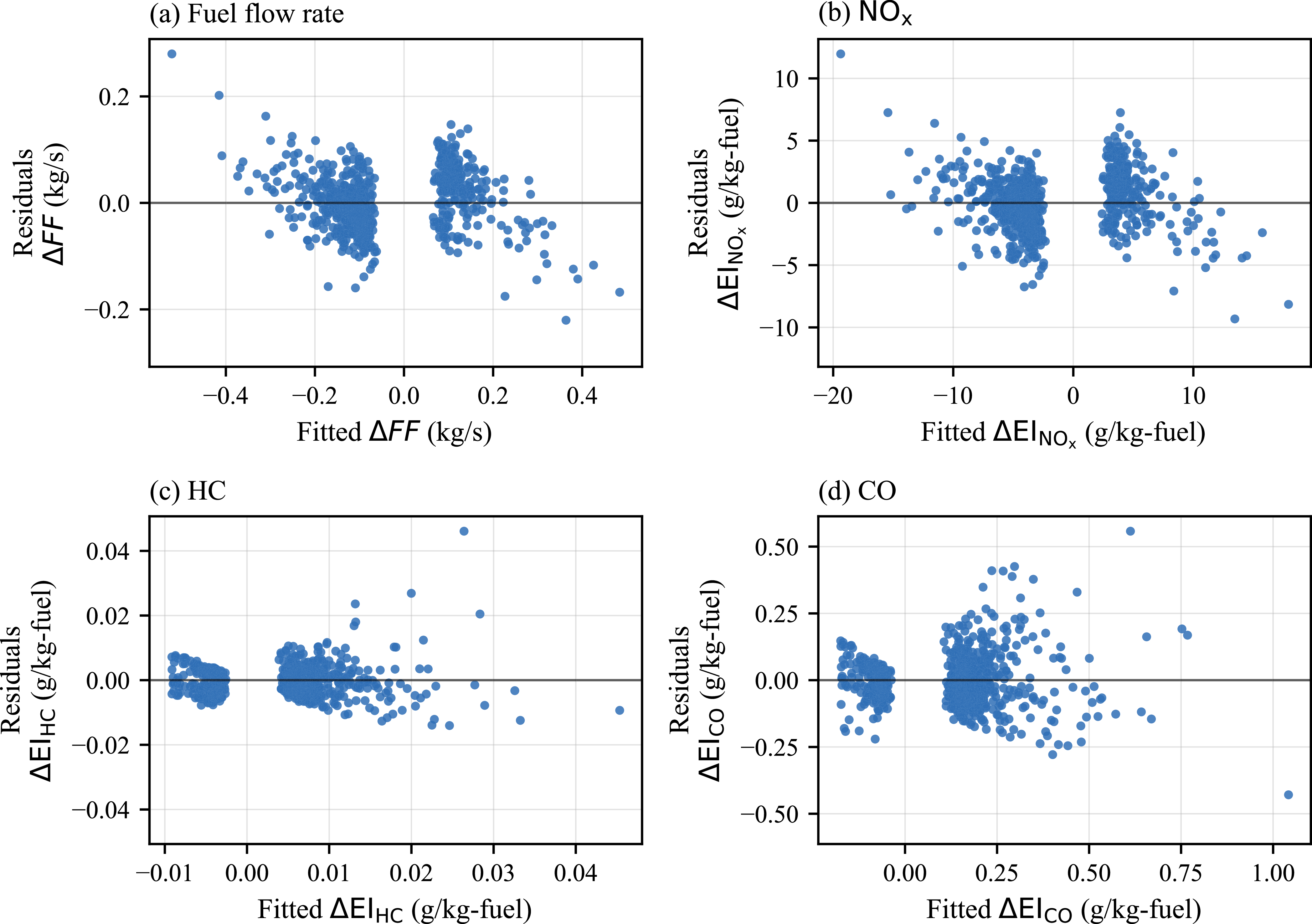
Residual diagnostics were then conducted by examining residuals against fitted values, as shown in Figure 16, and by applying the Breusch–Pagan test for heteroscedasticity. The residuals were generally distributed around zero across the range of speed changes, indicating no clear systematic overprediction or underprediction. 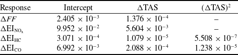However, the residual spread was not constant across the fitted-value range, particularly for the $\Delta \mathrm{EI}_{\mathrm{HC}}$ and $\Delta \mathrm{EI}_{\mathrm{CO}}$ models. This visual pattern was consistent with the Breusch–Pagan test, which indicated evidence of heteroscedasticity for all four models, with stronger evidence for HC and CO. Therefore, HC3 heteroscedasticity-robust standard errors were calculated for the regression coefficients. The resulting HC3 robust standard errors are summarised in Table 5.

Table 5.

HC3 heteroscedasticity-robust standard errors of the regression coefficients

Table 5. Long description

A table summarizing HC3 heteroscedasticity-robust standard errors of regression coefficients. The table has four rows and four columns. The columns are labeled Response, Intercept, ΔTAS, and (ΔTAS) squared. The rows are labeled with different responses: ΔFF, ΔEI_NOx, ΔEI_HC, and ΔEI_CO. Each cell contains numerical values representing the standard errors. Row 1: ΔFF, 2.405 x 10^-3, 1.376 x 10^-4, -. Row 2: ΔEI_NOx, 9.952 x 10^-2, 5.604 x 10^-3, -. Row 3: ΔEI_HC, 3.071 x 10^-4, 1.079 x 10^-5, 5.508 x 10^-7. Row 4: ΔEI_CO, 6.992 x 10^-3, 2.088 x 10^-4, 1.238 x 10^-5.

Figure 16.

Residuals versus fitted values for the regression models: (a) $\Delta FF$ , (b) $\Delta \mathrm{EI}_{\mathrm{NO_x}}$ , (c) $\Delta \mathrm{EI}_{\mathrm{HC}}$ and (d) $\Delta \mathrm{EI}_{\mathrm{CO}}$ .

Figure 16. Long description

Panel A: A scatter plot showing residuals of fuel flow rate against fitted values. The x-axis is labeled ‘Fitted ΔFF (kg/s)’ and the y-axis is labeled ‘Residuals ΔFF (kg/s)’. The data points are scattered around the zero line. Panel B: A scatter plot showing residuals of NOx against fitted values. The x-axis is labeled ‘Fitted ΔElNOx (g/kg-fuel)’ and the y-axis is labeled ‘Residuals ΔElNOx (g/kg-fuel)’. The data points are scattered around the zero line. Panel C: A scatter plot showing residuals of HC against fitted values. The x-axis is labeled ‘Fitted ΔElHC (g/kg-fuel)’ and the y-axis is labeled ‘Residuals ΔElHC (g/kg-fuel)’. The data points are scattered around the zero line. Panel D: A scatter plot showing residuals of CO against fitted values. The x-axis is labeled ‘Fitted ΔElCO (g/kg-fuel)’ and the y-axis is labeled ‘Residuals ΔElCO (g/kg-fuel)’. The data points are scattered around the zero line.

After applying heteroscedasticity-robust standard errors, the speed-change coefficients remained statistically significant for all models. In the $\Delta \mathrm{EI}_{\mathrm{HC}}$ and $\Delta \mathrm{EI}_{\mathrm{CO}}$ models, both the linear ( $\Delta \mathrm{TAS}$ ) and quadratic ( $(\Delta \mathrm{TAS})^2$ ) terms remained statistically significant, supporting the inclusion of quadratic terms in these models.

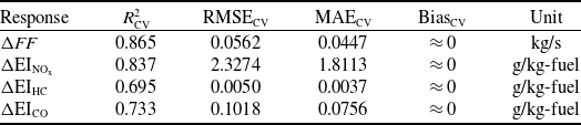
To assess predictive performance on unseen flights, grouped five-fold cross-validation was conducted using the FDR file identifier as the grouping variable. Thus, all manoeuvre observations from the same flight were assigned to the same fold and were not split between the training and validation sets. This reduces the risk of data leakage between manoeuvres from the same flight. The dataset contained 699 manoeuvre observations from 581 unique flights. The resulting cross-validated performance metrics are summarised in Table 6.

Table 6.

Grouped 5-fold cross-validation performance metrics of the regression models

Table 6. Long description

A table comparing grouped 5-fold cross-validation performance metrics of regression models. The table has 4 rows and 5 columns. Column headers are Response, R squared sub CV, RMSE sub CV, MAE sub CV, and Bias sub CV. Row 1: Response, Delta FF, Unit, kg/s. Row 2: R squared sub CV, 0.865, RMSE sub CV, 0.0562, MAE sub CV, 0.0447, Bias sub CV, approximately 0. Row 3: Response, Delta EI sub NOx, Unit, g/kg-fuel. Row 4: R squared sub CV, 0.837, RMSE sub CV, 2.3274, MAE sub CV, 1.8113, Bias sub CV, approximately 0. Row 5: Response, Delta EI sub HC, Unit, g/kg-fuel. Row 6: R squared sub CV, 0.695, RMSE sub CV, 0.0050, MAE sub CV, 0.0037, Bias sub CV, approximately 0. Row 7: Response, Delta EI sub CO, Unit, g/kg-fuel. Row 8: R squared sub CV, 0.733, RMSE sub CV, 0.1018, MAE sub CV, 0.0756, Bias sub CV, approximately 0.

The cross-validated results were close to the corresponding in-sample metrics, indicating that the regression models maintained similar performance on unseen flight groups. The $\Delta FF$ and $\Delta \mathrm{EI}_{\mathrm{NO_x}}$ models showed the strongest cross-validated performance, with $R^2_{\mathrm{CV}}$ values of 0.865 and 0.837, respectively. The $\Delta \mathrm{EI}_{\mathrm{HC}}$ and $\Delta \mathrm{EI}_{\mathrm{CO}}$ models showed more moderate performance, with $R^2_{\mathrm{CV}}$ values of 0.695 and 0.733, respectively. These results support the predictive usefulness of $\Delta \mathrm{TAS}$ , while also confirming that HC and CO responses exhibit greater variability.

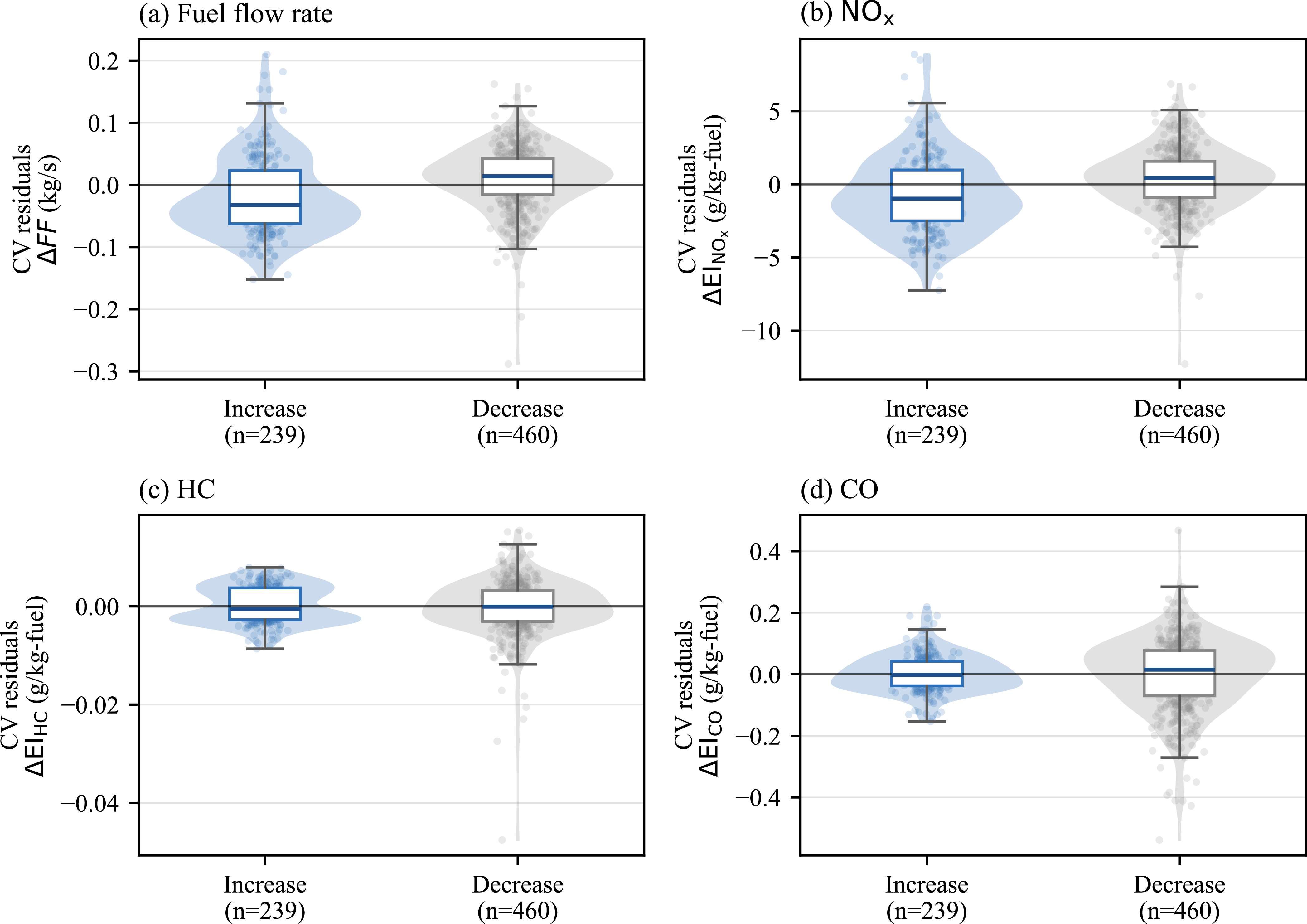
Robustness was further examined across manoeuvre direction, flight-level range and aircraft–engine configuration. Manoeuvre direction robustness was assessed by examining grouped cross-validated residual distributions separately for speed-increase and speed-decrease manoeuvres, as shown in Figure 17. The residual distributions were generally centred close to zero, suggesting that the models captured the overall response to signed speed changes across both acceleration and deceleration manoeuvres. However, $\Delta FF$ and $\Delta \mathrm{EI}_{\mathrm{NO_x}}$ showed a tendency toward negative residuals for speed-increase manoeuvres, indicating slight underprediction in acceleration cases. For $\Delta \mathrm{EI}_{\mathrm{HC}}$ and $\Delta \mathrm{EI}_{\mathrm{CO}}$ , the median residuals were closer to zero, although the spread of residuals differed between manoeuvre directions. These results suggest that manoeuvre direction introduces some variability, but does not invalidate the overall modelling approach.

Figure 17.

Grouped cross-validated residual distributions by manoeuvre direction for the regression models: (a) $\Delta FF$ , (b) $\Delta \mathrm{EI}_{\mathrm{NO_x}}$ , (c) $\Delta \mathrm{EI}_{\mathrm{HC}}$ and (d) $\Delta \mathrm{EI}_{\mathrm{CO}}$ . Residuals are defined as predicted values minus observed values. Violin shapes show the residual distributions, boxplots show the median and interquartile range and points represent individual manoeuvre observations.

Figure 17. Long description

Panel A: A violin plot with a box plot shows the distribution of cross-validated residuals for fuel flow rate (kg/s) by manoeuvre direction. The x-axis labels are Increase (n=239) and Decrease (n=460), and the y-axis is labeled CV residuals ΔFF (kg/s). Panel B: A violin plot with a box plot displays the distribution of cross-validated residuals for NOx emissions (g/kg-fuel) by manoeuvre direction. The x-axis labels are Increase (n=239) and Decrease (n=460), and the y-axis is labeled CV residuals ΔEINOx (g/kg-fuel). Panel C: A violin plot with a box plot illustrates the distribution of cross-validated residuals for HC emissions (g/kg-fuel) by manoeuvre direction. The x-axis labels are Increase (n=239) and Decrease (n=460), and the y-axis is labeled CV residuals ΔEIHC (g/kg-fuel). Panel D: A violin plot with a box plot presents the distribution of cross-validated residuals for CO emissions (g/kg-fuel) by manoeuvre direction. The x-axis labels are Increase (n=239) and Decrease (n=460), and the y-axis is labeled CV residuals ΔEICO (g/kg-fuel).

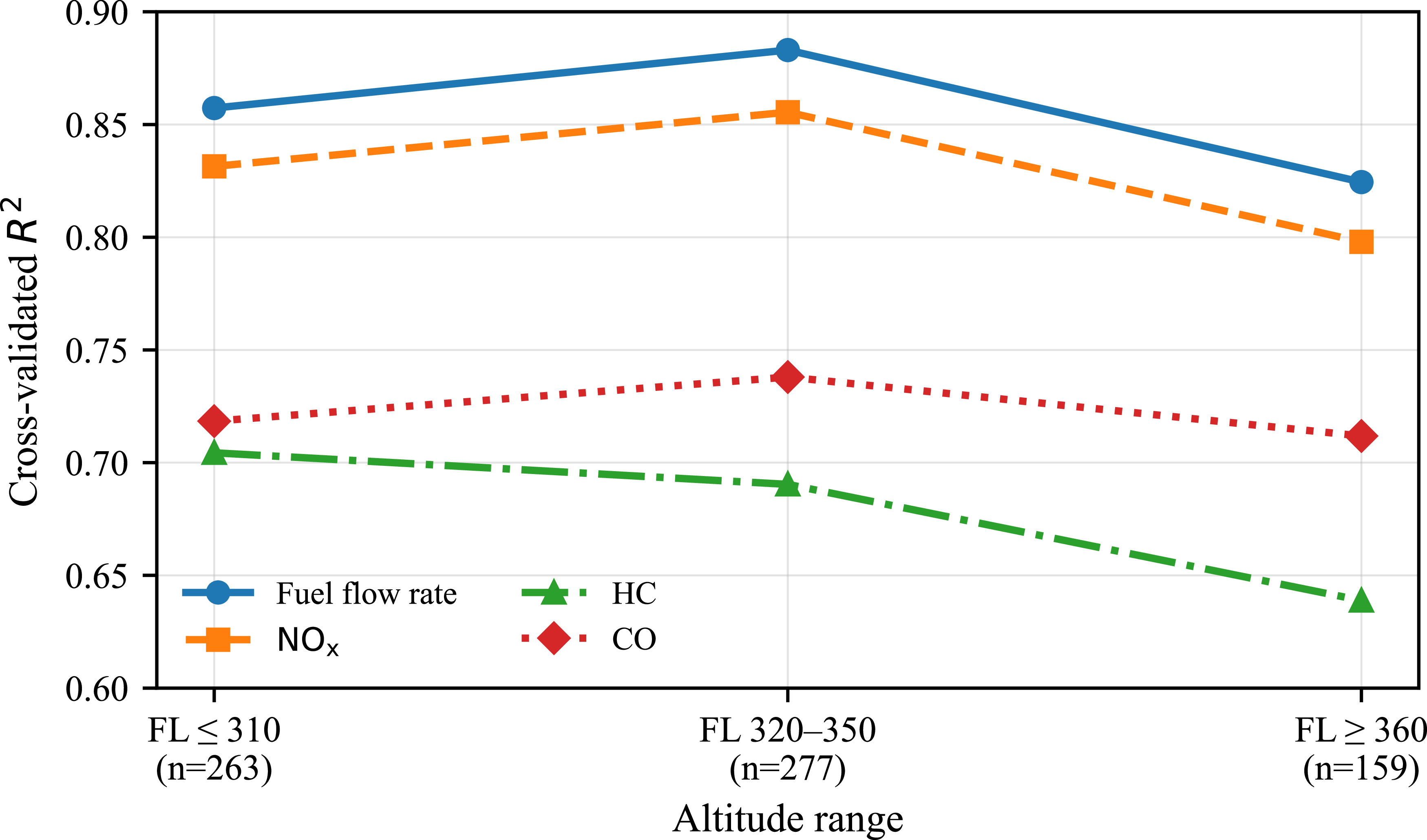
Altitude-based robustness was assessed by evaluating the grouped cross-validated predictions across three flight-level ranges, as shown in Figure 18. The $\Delta FF$ and $\Delta \mathrm{EI}_{\mathrm{NO_x}}$ models showed consistently strong performance across altitude ranges, with only a modest reduction at higher FLs. The $\Delta \mathrm{EI}_{\mathrm{HC}}$ and $\Delta \mathrm{EI}_{\mathrm{CO}}$ models showed more moderate but broadly comparable performance across the three altitude bands. Overall, the results indicate that the main speed-change relationships were reasonably stable across the altitude range represented in the dataset.

Figure 18.

Cross-validated coefficient of determination, $R^2_{\mathrm{CV}}$ , across flight-level ranges. The values were calculated from grouped cross-validated predictions within each flight-level band.

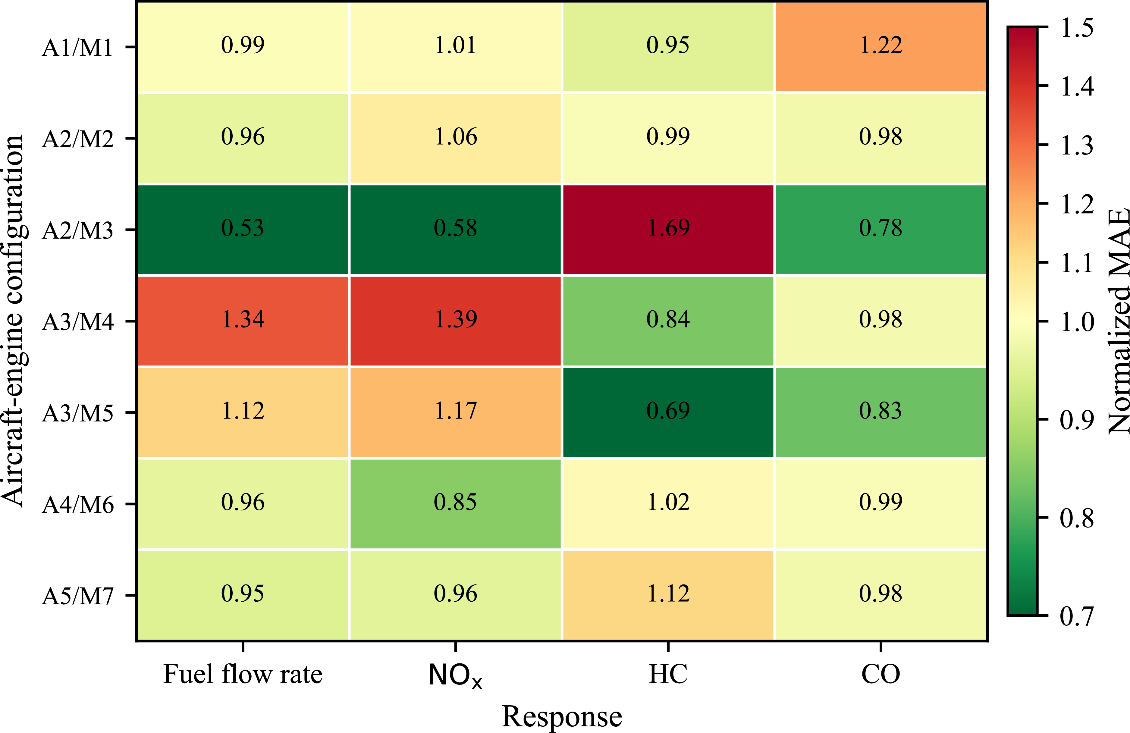
Aircraft–engine configuration robustness was evaluated using the subgroup MAE normalised by the corresponding overall cross-validated MAE, as shown in Figure 19. Values close to 1.0 indicate that the subgroup prediction error is comparable to the overall model error, whereas values greater than 1.0 indicate higher subgroup prediction error. The $\Delta FF$ and $\Delta \mathrm{EI}_{\mathrm{NO_x}}$ models showed broadly consistent performance across most aircraft–engine configurations, although somewhat higher normalised errors were observed for the A3/M4 configuration. The $\Delta \mathrm{EI}_{\mathrm{CO}}$ model also remained relatively stable across configurations. In contrast, $\Delta \mathrm{EI}_{\mathrm{HC}}$ showed greater subgroup variability, particularly for the A2/M3 configuration. This result should be interpreted cautiously because this subgroup contained only 24 observations. Overall, the robustness check indicates that the main speed-change relationships are reasonably stable across aircraft–engine configurations, while HC responses are more sensitive to configuration-specific effects.

Figure 19.

Normalised grouped cross-validated MAE across aircraft–engine configurations. Values are calculated as $\mathrm{MAE}_{\mathrm{subgroup}}/\mathrm{MAE}_{\mathrm{overall}}$ ; values near 1 indicate performance comparable to the overall model.

3.4 Stepwise benchmark comparison with multivariable models

The proposed $\Delta \mathrm{TAS}$ -based models were compared with stepwise multivariable benchmark models. The benchmark analysis was conducted for all response variables considered in this study, namely $\Delta FF$ , $\Delta \mathrm{EI}_{\mathrm{NO_x}}$ , $\Delta \mathrm{EI}_{\mathrm{HC}}$ and $\Delta \mathrm{EI}_{\mathrm{CO}}$ . For $\Delta FF$ and $\Delta \mathrm{EI}_{\mathrm{NO_x}}$ , the baseline model included $\Delta \mathrm{TAS}$ . For $\Delta \mathrm{EI}_{\mathrm{HC}}$ and $\Delta \mathrm{EI}_{\mathrm{CO}}$ , the quadratic speed-change term was retained, consistent with the original model specification. Additional predictors were then introduced stepwise: $FL$ , aircraft mass before the manoeuvre ( $m_0$ ), initial true airspeed ( $\mathrm{TAS}_0$ ), ambient temperature before the manoeuvre ( $T_{\mathrm{amb},0}$ ) and aircraft type.

The comparison was performed using grouped five-fold cross-validation, with the FDR file identifier used as the grouping variable. This ensured that manoeuvre observations originating from the same flight were not split between training and validation folds. Model performance was evaluated using the cross-validated coefficient of determination $R^2_{\mathrm{CV}}$ and the mean absolute error $\mathrm{MAE}_{\mathrm{CV}}$ . Since the four response variables have different physical units and numerical scales, $\mathrm{MAE}_{\mathrm{CV}}$ was also normalised by the corresponding baseline $\mathrm{MAE}_{\mathrm{CV}}$ obtained using only $\Delta \mathrm{TAS}$ as a predictor for each response variable.

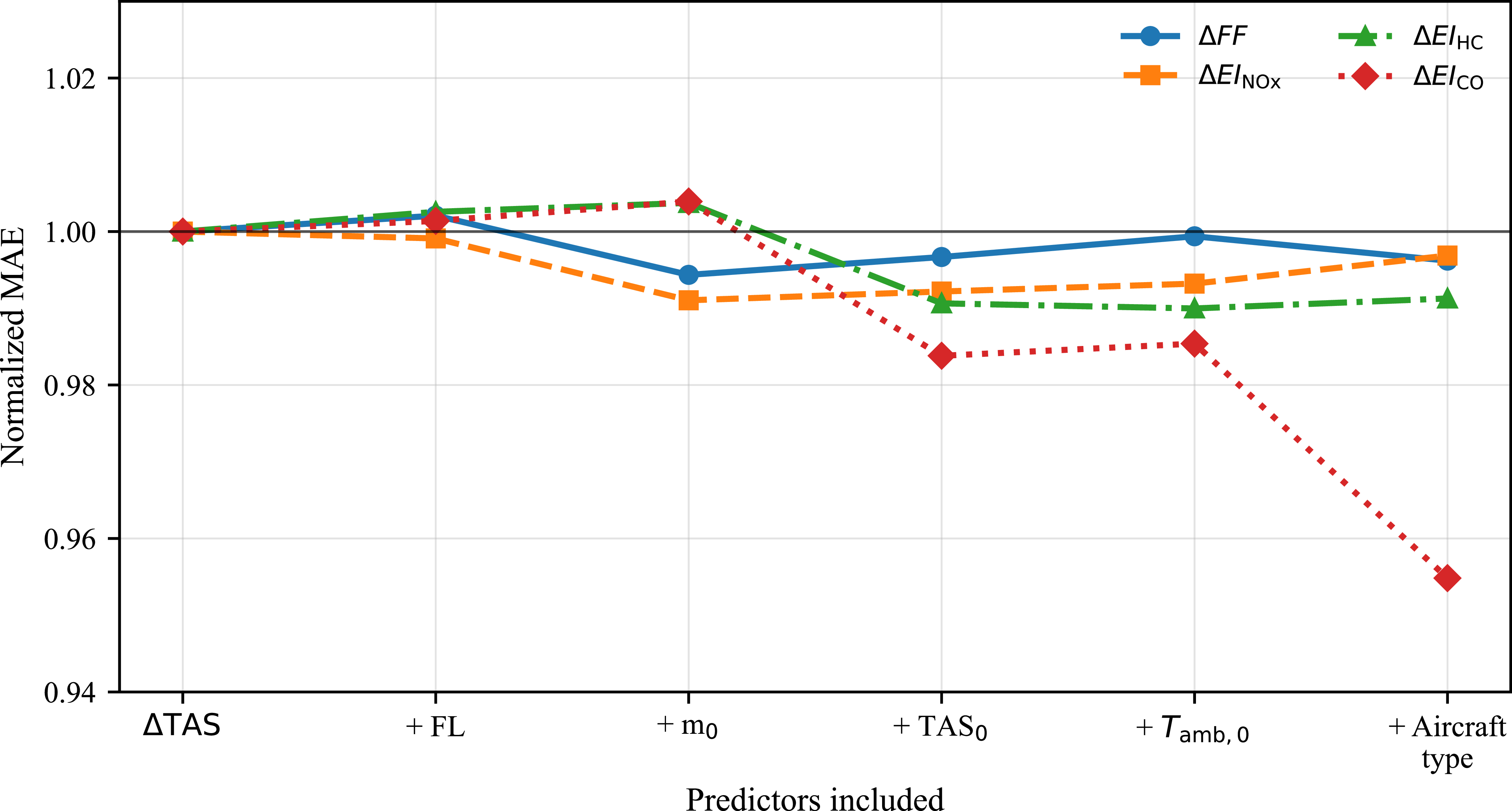
The stepwise comparisons of grouped cross-validated $R^2$ and normalised $\mathrm{MAE}_{\mathrm{CV}}$ are shown in Figures 20 and 21, respectively.

Figure 20.

Stepwise comparison of grouped cross-validated $R^2$ values as additional predictors are introduced to the baseline model using $\Delta \mathrm{TAS}$ .

Figure 21.

Stepwise comparison of normalised $\mathrm{MAE}_{\mathrm{CV}}$ values as additional predictors are introduced to the baseline model using $\Delta \mathrm{TAS}$ . For each response variable, normalized MAE_CV is calculated as the ratio of the model’s $\mathrm{MAE}_{\mathrm{CV}}$ to the $\mathrm{MAE}_{\mathrm{CV}}$ of the baseline model using only $\Delta \mathrm{TAS}$ . Values below 1 indicate lower prediction error than the baseline model.

As shown in Figure 20, the additional predictors did not materially improve the prediction of $\Delta FF$ or $\Delta \mathrm{EI}_{\mathrm{NO_x}}$ . For $\Delta FF$ , the $R^2_{\mathrm{CV}}$ value changed from 0.8651 for the speed-change-only model to 0.8643 for the full multivariable model. Similarly, for $\Delta \mathrm{EI}_{\mathrm{NO_x}}$ , the corresponding values were 0.8373 and 0.8355. The normalised error trends in Figure 21 also show that $\mathrm{MAE}_{\mathrm{CV}}$ remained nearly unchanged for these two responses. These results indicate that signed speed change captured most of the explainable manoeuvre-level variation in $\Delta FF$ and $\Delta \mathrm{EI}_{\mathrm{NO_x}}$ in the present dataset.

For $\Delta \mathrm{EI}_{\mathrm{HC}}$ and $\Delta \mathrm{EI}_{\mathrm{CO}}$ , the multivariable models provided modest improvements. The $R^2_{\mathrm{CV}}$ value for $\Delta \mathrm{EI}_{\mathrm{HC}}$ increased from 0.6951 to 0.7088, while that for $\Delta \mathrm{EI}_{\mathrm{CO}}$ increased from 0.7330 to 0.7613. The normalised $\mathrm{MAE}_{\mathrm{CV}}$ comparison shows a clearer reduction in prediction error for $\Delta \mathrm{EI}_{\mathrm{CO}}$ , whereas the improvement for $\Delta \mathrm{EI}_{\mathrm{HC}}$ was smaller. This suggests that HC and CO responses are more sensitive to additional operating-condition and aircraft-type effects than $\Delta FF$ and $\Delta \mathrm{EI}_{\mathrm{NO_x}}$ .

3.5 Evaluation of direction interaction and aircraft type effects

To examine whether models using only $\Delta \mathrm{TAS}$ as a predictor omitted systematic differences between acceleration and deceleration, manoeuvre direction interaction models were evaluated. These models allowed the response to signed net true-airspeed change to differ between speed-increase and speed-decrease manoeuvres. The linear structure was retained for $\Delta FF$ and $\Delta \mathrm{EI}_{\mathrm{NO_x}}$ , whereas the quadratic structure was retained for $\Delta \mathrm{EI}_{\mathrm{HC}}$ and $\Delta \mathrm{EI}_{\mathrm{CO}}$ .

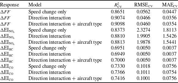
Each interaction model was also extended with aircraft-type fixed effects to account for systematic average differences among aircraft types without estimating separate speed-change relationships for every aircraft–engine configuration. This approach was preferred to fully stratified models because the configuration subgroups were unbalanced and some contained relatively few observations. All benchmark models were evaluated using grouped five-fold cross-validation, with the FDR file identifier used as the grouping variable to ensure that observations from the same flight were not split between training and validation folds. The results are summarised in Table 7.

Table 7.

Grouped 5-fold cross-validation comparison of speed change only, direction interaction and aircraft type fixed effect models

Table 7. Long description

The table presents a comparison of three models: speed change only, direction interaction, and direction interaction plus aircraft type fixed effects. It includes five responses: delta FF, delta EI NOx, delta EI HC, and delta EI CO. The table has 15 rows and 5 columns. Column headers are Response, Model, R squared CV, RMSE CV, and MAE CV. Row labels include different models for each response. Each row provides the R squared CV, RMSE CV, and MAE CV values for the corresponding model and response. Notable trends include varying performance across different models and responses, with some models showing lower RMSE CV and MAE CV values, indicating better performance.

RMSE and MAE are reported in the units of the corresponding response variable.

The manoeuvre direction interaction improved the prediction of $\Delta FF$ and $\Delta \mathrm{EI}_{\mathrm{NO_x}}$ . Their grouped cross-validated $R^2$ values increased from 0.8651 to 0.9074 and from 0.8373 to 0.8810, respectively, while the corresponding $\mathrm{MAE}_{\mathrm{CV}}$ values decreased from 0.0447 to 0.0356 kg/s and from 1.8113 to 1.5426 g/kg-fuel. Adding aircraft-type fixed effects produced only marginal further changes in these metrics.

For $\Delta \mathrm{EI}_{\mathrm{HC}}$ and $\Delta \mathrm{EI}_{\mathrm{CO}}$ , the interaction and aircraft-type extensions provided little or no improvement. Thus, the models using only $\Delta \mathrm{TAS}$ as a predictor remain compact first-order approximations, whereas the direction interaction formulation offers a more accurate alternative for fuel flow rate and $\mathrm{NO_x}$ .

3.6 Sensitivity analysis

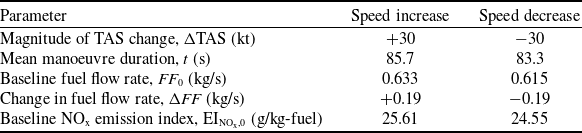
Although HC and CO emission indices exhibit nonlinear and asymmetric responses to speed changes, they are predominantly associated with low-thrust operating conditions, and their absolute magnitudes remain considerably smaller than those of $\mathrm{NO_x}$ emissions. Consequently, the sensitivity analysis focuses on fuel consumption and $\mathrm{NO_x}$ emissions using the fixed input values summarised in Table 8. The baseline fuel flow rate and baseline $\mathrm{NO_x}$ emission index values in Table 8 were selected as the mean pre-manoeuvre values from the analysed dataset, separately for speed-increase and speed-decrease cases. These values represent global direction-specific averages across all aircraft–engine configurations. For speed increases and decreases, respectively, the standard deviations were 0.074 and 0.059 kg/s for baseline fuel flow rate and 4.09 and 3.65 g/kg-fuel for the baseline $\mathrm{NO_x}$ emission index. For the representative 30 kt case, manoeuvre duration was estimated by scaling the direction-specific ratio of mean manoeuvre duration to mean absolute speed change to 30 kt. When individual manoeuvres were normalised to an equivalent 30 kt change, the corresponding duration standard deviations were 22.6 s for speed increases and 27.7 s for speed decreases.

Table 8.

Input values used in the sensitivity analysis for a representative 30 kt speed change manoeuvre

Table 8. Long description

A table with four rows and six columns comparing parameters for speed increase and decrease in a sensitivity analysis. The columns are labeled Parameter, Speed increase, and Speed decrease. The rows are labeled Magnitude of TAS change, Mean manoeuvre duration, Baseline fuel flow, Change in fuel flow, and Baseline emission index. Row 1: Magnitude of TAS change, (kt), +30, -30. Row 2: Mean manoeuvre duration, (s), 85.7, 83.3. Row 3: Baseline fuel flow, (kg/s), 0.633, 0.615. Row 4: Change in fuel flow, (kg/s), +0.19, -0.19. Row 5: Baseline emission index, (g/kg-fuel), 25.61, 24.55.

Baseline fuel flow rate and $\mathrm{NO_x}$ emission index values correspond to mean pre-manoeuvre values calculated separately for speed increase and speed decrease cases.

The 10, 20 and 30 kt cases were selected to represent small, moderate and relatively large tactical speed changes. This choice is consistent with operational speed-control practice, as ICAO also states that speed adjustments should be expressed in increments of 0.01 Mach at or above FL250 and 10 kt indicated airspeed (IAS) below FL250 [30]. Although the present analysis is based on changes in TAS rather than controller-issued Mach or IAS instructions, these values provide representative sensitivity magnitudes for assessing the fuel and $\mathrm{NO_x}$ effects of tactical speed manoeuvres.

Fuel flow rates and emission indices during speed manoeuvres are obtained by applying regression models to baseline conditions derived from pre-manoeuvre flight segments. These elements are then combined to estimate the cumulative change in $\mathrm{NO_x}$ mass associated with a speed manoeuvre.

The fuel flow regression model indicates a sensitivity of approximately $6.31\times 10^{-3}$ kg/s per kt of TAS change, as given by Equation (12). Accordingly, a 30 kt speed increase corresponds to an average fuel flow rate increase of approximately 0.19 kg/s. Based on the observed speed-change dynamics, the mean manoeuvre duration is approximately 85.7 s for speed increases and 83.3 s for speed reductions, resulting in an estimated cumulative fuel penalty of about 16.3 kg for a 30 kt acceleration and a comparable fuel saving of approximately 15.8 kg for a 30 kt deceleration. The sensitivity of $\mathrm{NO_x}$ emissions is evaluated using the linear relationship between changes in the $\mathrm{NO_x}$ emission index and TAS variation given by Equation (13). For a representative 30 kt speed increase, the combined effect of increased fuel flow rate and an elevated $\mathrm{NO_x}$ emission index leads to an estimated $\mathrm{NO_x}$ penalty of approximately 0.92 kg. In contrast, a 30 kt speed reduction results in an estimated $\mathrm{NO_x}$ saving of approximately 0.64 kg. The cumulative $\mathrm{NO_x}$ change is computed as the difference between manoeuvre and baseline emissions, each calculated using the ICAO formulation in Equation (11). 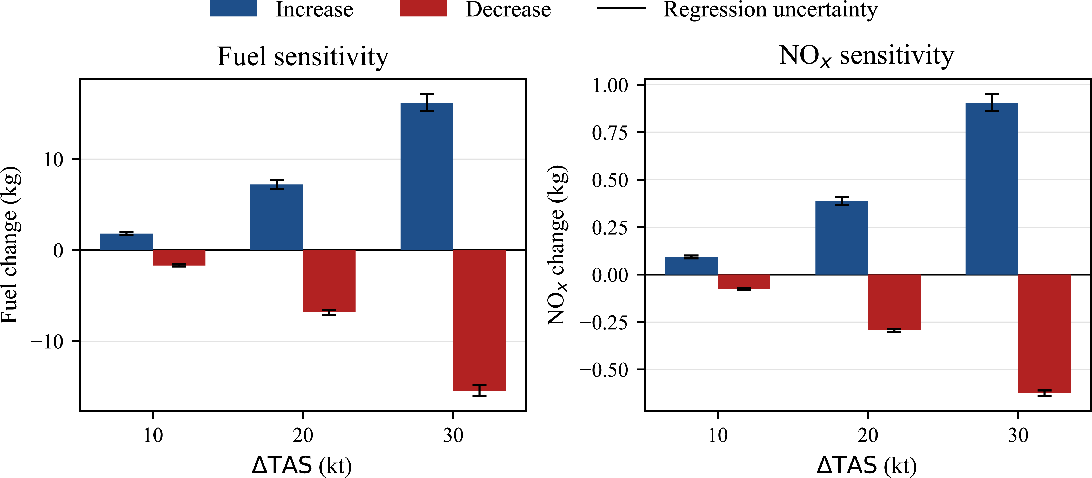Corresponding fuel consumption and $\mathrm{NO_x}$ emission sensitivities are also computed for 10 and 20 kt speed changes, together with the representative 30 kt case, as shown in Figure 22.

Figure 22.

Sensitivity of fuel consumption and $\mathrm{NO_x}$ emissions to different speed manoeuvres. Error bars indicate approximate 95% uncertainty intervals obtained from Monte Carlo propagation of regression-coefficient uncertainty.

Uncertainty in the regression equations was propagated into the cumulative fuel and $\mathrm{NO_x}$ estimates using Monte Carlo sampling of the regression coefficients from their HC3 robust covariance matrices. For each sampled coefficient set, $\Delta FF$ , $\Delta \mathrm{EI}_{\mathrm{NO_x}}$ , cumulative fuel change and cumulative $\mathrm{NO_x}$ change were recalculated. The resulting 95% uncertainty intervals are shown in Figure 22. The intervals remain relatively narrow and do not cross zero, indicating that the sign of the estimated effect is robust. For the representative 30 kt case, the estimated fuel change is 16.17 kg [15.22, 17.12] for acceleration and −15.43 kg [−16.01, −14.84] for deceleration, while the corresponding $\mathrm{NO_x}$ changes are 0.906 kg [0.861, 0.951] and −0.624 kg [−0.639, −0.610], respectively.

The potential effect of manoeuvre-duration variability was also examined separately. When manoeuvre duration, baseline fuel flow rate and baseline $\mathrm{NO_x}$ emission index were sampled from their empirical direction-specific distributions, the uncertainty ranges became wider. For example, for the 30 kt acceleration case, the estimated fuel change ranged from 9.53 to 27.27 kg, while the corresponding $\mathrm{NO_x}$ change ranged from 0.486 to 1.524 kg. For the 30 kt deceleration case, the estimated fuel saving ranged from 8.81 to 27.82 kg, and the $\mathrm{NO_x}$ saving ranged from 0.334 to 1.219 kg. These results indicate that manoeuvre-duration variability can materially affect the magnitude of cumulative fuel and $\mathrm{NO_x}$ estimates. However, the main objective of this study is to develop empirical regression models for fuel flow and emission-index changes during speed manoeuvres. A more detailed manoeuvre-duration prediction model is therefore left for future work.

The results provide a quantitative basis for exploring the implications of fuel and $\mathrm{NO_x}$ considerations in air traffic management, including their potential role in speed-based conflict resolution. The observed asymmetry between acceleration and deceleration indicates that speed reductions generally offer lower environmental costs, suggesting that environmentally aware conflict resolution strategies should preferentially exploit deceleration-based manoeuvres where feasible. However, the use of speed reductions may introduce operational trade-offs. Prolonged reductions can increase flight time and delay risk, which may be incompatible with airline operating procedures or cost index policies that balance time-related costs against fuel consumption. Consequently, speed reductions may not be universally acceptable from an airline perspective, particularly when delay penalties outweigh potential fuel and $\mathrm{NO_x}$ savings.