2.0 Background

As described in Reference [Reference Poll and Schumann4], starting with the engine overall efficiency, $\eta$ _o , defined as

(1) \begin{equation}\eta _{o}=\frac{nF_{\!n}V_{\infty }}{\dot{m}_{f}LCV}\end{equation}

where n is the number of engines, F _n is the net, installed thrust per engine, V $ _{\infty} $ is the true airspeed, $\dot{m}_{f}$ is the fuel mass flow per unit time and LCV is the lower calorific value of the fuel, the instantaneous SAR is given by

(2) \begin{equation}SAR=\frac{dS}{dm_{f}}=\frac{V_{\infty }}{\dot{m}_{f}}=\left(\frac{D}{nF_{\!n}}\right)\left(\frac{\left(\eta _{o}L/D\right)LCV}{L}\right)\end{equation}

Here, S is the distance travelled through the air, L is the total lift, and D is the total drag.

In the steady-state cruise, lift is equal to weight and thrust is equal to drag.Footnote ² Hence,

(3) \begin{equation}\frac{dS}{dm_{f}}=-\frac{dS}{dm}=\left(\frac{\left(\eta _{o}L/D\right)LCV}{mg}\right)\end{equation}

where m is the instantaneous total mass of the aircraft and g is the acceleration due to gravity. Therefore, in cruise, the SAR is governed by the instantaneous mass, m, and the single aero-thermodynamic parameter ( $\eta$ _o L/D). For this reason, ( $\eta$ _o L/D) is sometimes referred to as the ‘range parameter’ (see, for example, Torenbeeck [Reference Torenbeek5]).

In normal operations, aircraft do not cruise at specific values of geometric altitude. Rather, to maintain safe separation in the vertical direction, they follow isobars, i.e. the altitude is constantly modulated so that the local static pressure, p $ _{\infty} $ , is held constant. By international agreement, values of local static pressure are converted into non-dimensional FLs. These are the geopotential altitudes, measured in feet, that the aircraft would have if it were operating in the ISA [1] made non-dimensional by dividing by 100 feet. For example, if the local static pressure measured by the aircraft air data system is 238.42 hPa, the geopotential altitude in the ISA would be 35,000 feet and, hence, the aircraft would be flying at FL 350.

3.0 Conditions for optimum ( $\eta$ _o L/D) and the design optimum

In Poll and Schumann [Reference Poll and Schumann2], it was shown that, for a given aircraft operating at fixed Mach number in steady, straight and level flight, there is a lift coefficient, (C _L ) _B , at which ( $\eta$ _o L/D) has a local maximum, or best, value. Furthermore, there is a particular Mach number and lift coefficient combination at which ( $\eta$ _o L/D) reaches an absolute maximum, or optimum, level. The conditions for optimum ( $\eta$ _o L/D) are determined by a balance between the gradients of $\eta$ _o and L/D with respect to both Mach number, M $ _{\infty} $ , and either FL or local static pressure, p $ _{\infty} $ , i.e. when

(4) \begin{equation}d\left(\eta _{o}L/D\right)=\frac{\partial \left(\eta _{o}L/D\right)}{\partial M_{\infty }}dM_{\infty }+\frac{\partial \left(\eta _{o}L/D\right)}{\partial p_{\infty }}dp_{\infty }=0\end{equation}

In a steady, straight and level cruise, using the usual definitions for the aircraft lift, drag and thrust coefficients,

(5) \begin{equation}C_{L}=\frac{L}{q_{\infty }S_{ref}}\approx \frac{mg}{q_{\infty }S_{ref}} \ \mathrm{and} \ C_{D}=\frac{D}{q_{\infty }S_{ref}} \ \approx \ C_{T}=\frac{nF_{\!n}}{q_{\infty }S_{ref}}\end{equation}

where S _ref is the wing reference area and, if γ is the ratio of specific heats for air,

(6) \begin{equation}q_{\infty }=\frac{\gamma }{2} \ p_{\infty }{M}_{\infty }^{2}\end{equation}

Combining Equations (5) and (6) and taking m to be constant, partial differentiation of the lift coefficient with respect to M $ _{\infty} $ and p $ _{\infty} $ gives

(7) \begin{equation} \ \frac{M_{\infty }}{C_{L}}\left(\frac{\partial C_{L}}{\partial M_{\infty }}\right)^{p}= -2 \ \text{and } \ \frac{p_{\infty }}{C_{L}}\left(\frac{\partial C_{L}}{\partial p_{\infty }}\right)^{M}=-1 \ \end{equation}

Here, the superscripts p and M indicate derivatives at constant static pressure and constant Mach number, respectively. Therefore, Equation (4) is satisfied when

(8) \begin{equation}\frac{M_{\infty }}{\eta _{o}}\frac{\partial \eta _{o}}{\partial M_{\infty }}-\frac{M_{\infty }}{Cd}\frac{\partial C_{D}}{\partial M_{\infty }}-2=0\end{equation}

and

(9) \begin{equation}\frac{C_{L}}{C_{D}}\frac{\partial C_{D}}{\partial C_{L}}\left(1-\frac{C_{T}}{\eta _{o}}\frac{\partial \eta _{o}}{\partial C_{T}}\right)-1=0\end{equation}

As described in Poll and Schumann [Reference Poll and Schumann2], the drag coefficient, C _D , is a function of aircraft geometry, C _L , M $ _{\infty} $ and the Reynolds number, $R^{ac}$ , where

(10) \begin{equation}R^{ac}=\frac{l\rho _{\infty }V_{\infty }}{\mu _{\infty }}={S}_{ref}^{1/2}\left(\frac{\gamma p_{\infty }M_{\infty }}{{a_{\infty }}\mu _{\infty }}\right)\end{equation}

Here, ρ $ _{\infty} $ is the air density, a $ _{\infty} $ is the local speed of sound and μ $ _{\infty} $ is the air dynamic viscosity. It follows that

(11) \begin{equation}C_{D}=C_{D}\left(C_{L},M_{\infty }\mathrm{and} \ R^{ac} \right)\end{equation}

Referring to the example shown in Figure 1, when the atmosphere is specified and the mass and flight Mach number are fixed, the aircraft lift-to-drag ratio has a local maximum at a particular value of the drag coefficient (and, hence, a particular lift coefficient). The maximum L/D reduces as the Mach number increases. In this case, C _D is varied by changing the FL.

Figure 1.

An example of the variation of aircraft lift-to-drag ratio with drag coefficient and Mach number in the ISA when the mass is fixed. Figure taken from Poll and Schumann [Reference Poll and Schumann2].

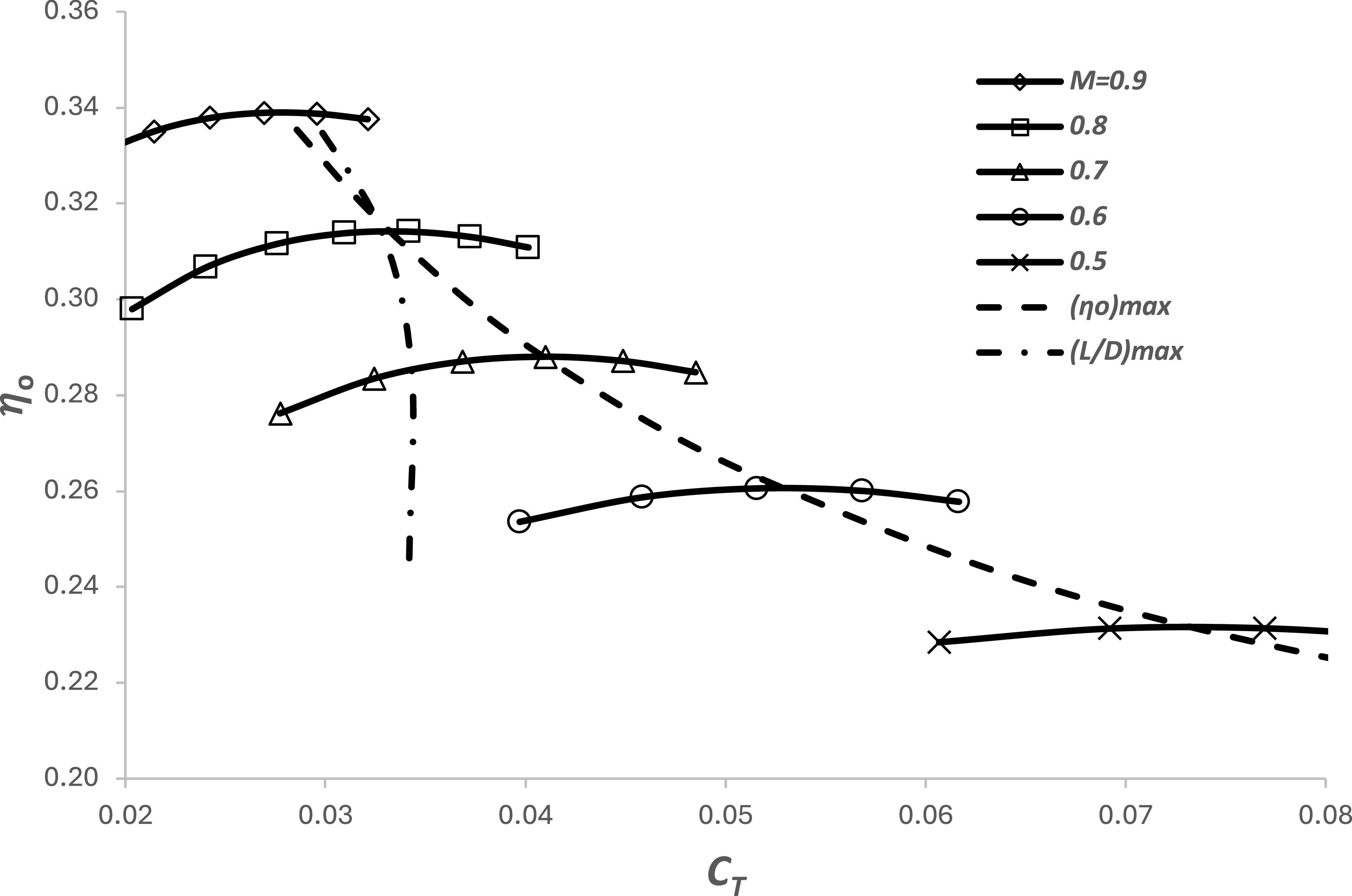
Similarly, as described in Poll and Schumann [Reference Poll and Schumann3] and as shown in Figure 2, at fixed M $ _{\infty} $ , engine overall efficiency, $\eta$ _o , has a local maximum value at a particular value of the thrust coefficient, C _T . This maximum value increases as the Mach number increases and, provided that M $ _{\infty} $ is greater than 0.2,Footnote ³ it may be represented by a power law, i.e. when

(12) \begin{align} \frac{C_{T}}{\eta _{o}}\frac{\partial \eta _{o}}{\partial C_{T}}=0 \quad \\[-10pt] \nonumber \end{align}

(13) \begin{align} \left(\eta _{o}\right)_{B}\approx \eta _{1}\left(M_{\infty }\right)^{{\eta _{2}}} \\[10pt] \nonumber \end{align}

where the coefficients $\eta$ ₁ and $\eta$ ₂ are constant and depend upon the engine type. It follows that

(14) \begin{equation}\left(\frac{M_{\infty }}{\eta _{o}}\frac{\partial \eta _{o}}{\partial M_{\infty }}\right)_{B}=\eta _{2}\end{equation}

Figure 2.

The variation of overall efficiency with drag (=thrust) coefficient and Mach number for a civil aircraft turbofan engine with a nominal bypass ratio of 8. Figure taken from Poll and Schumann [Reference Poll and Schumann3].

In order to have the absolute maximum value of ( $\eta$ _o L/D), the airframe and engine must be perfectly matched, i.e. both $\eta$ _o and L/D must have local maxima at the same values of M $ _{\infty} $ and C _D (=C _T ). The locus of ( $\eta$ _o ) _max is shown in Figure 2 together with the locus of (L/D) _max cross-plotted from Figure 1. The absolute maximum value of ( $\eta$ _o L/D) occurs at the loci intersection point. In this example, this corresponds to an M $ _{\infty} $ of 0.8, C _D of 0.033, C _L of 0.528 and an ( $\eta$ _o L/D) of 5.03.

From the definition of the Reynolds number given in Equation (10) and noting that a $ _{\infty} $ and $\mu$ _∞ only depend upon temperature, when the variation of temperature with pressure in the atmosphere is specified,

(15) \begin{equation}{a_{\infty }}\mu _{\infty }=\textit{function}(\ \! p_{\infty})\end{equation}

Therefore,

(16) \begin{equation}p_{\infty }=\textit{function}\big(M_{\infty },R^{ac}\text{ and} \ S_{ref}\big)\end{equation}

From the definition of lift coefficient,

(17) \begin{equation}C_{L}=\frac{2mg}{ \ \gamma {p_{\infty }}{M}_{\infty }^{2}S_{ref}}=\textit{function}\big(m, {S_{ref}}, M_{\infty } \ \mathrm{and} \ R^{ac}\big)\end{equation}

and, from Equation (11),

(18) \begin{equation}C_{D}=C_{D}\big(C_{L}, M_{\infty } \ and \ R^{ac} \big)=\textit{function}\big(m, {S_{ref}}, M_{\infty } \ \mathrm{and} \ R^{ac}\big)\end{equation}

Hence, for a given aircraft and engine combination, operating in a specified, single-valued,Footnote ⁴ atmosphere, e.g. the ISA, at specified values of M _∞ , C _L and C _D , there is only one possible combination of mass, m, and R ^ac , i.e. one m and FL pair. Since this operating point is effectively determined in the design process, it is appropriate to call it the “design” optimum condition.

At the design optimum, Equations (12) and (14) apply, and Equations (8) and (9) become

(19) \begin{equation}\left(\frac{M_{\infty }}{C_{D}}\frac{\partial C_{D}}{\partial M_{\infty }}\right)_{DO}=\eta _{2}-2\end{equation}

and

(20) \begin{equation}\left(\frac{C_{L}}{C_{D}}\frac{\partial C_{D}}{\partial C_{L}}\right)_{DO}=1\end{equation}

These are completely general relations that define the design optimum value of ( $\eta$ _o L/D) for the design mass, m _des, in the specified design atmosphere and the conditions at which it occurs.

Whilst the actual design conditions are known only to the manufacturer, in Reference [Reference Poll and Schumann2], it was shown that, in general, the design optimum conditions can be expressed in terms of a mean skin-friction coefficient, C _F , defined as

(21) \begin{equation}{C}_{F}^{ac}\approx \frac{a}{\left(R^{ac}\right)^{b}}=\frac{0.0269}{\left(R^{ac}\right)^{0.14}}\end{equation}

and a parameter, ${\varGamma}$ , that captures the atmospheric effects (see Appendix A), i.e.

(22) \begin{equation} \ {\varGamma} \approx 38.97(1-\overline{{\unicode{x0394}} T})L_{h}\end{equation}

Here, L _h is the vertical temperature lapse with respect to geopotential height, having units of K/m and the temperature term

(23) \begin{equation} \ \ \overline{{\unicode{x0394}} T}=\frac{{\unicode{x0394}} T}{(T_{TP})_{ISA}}\end{equation}

where $\mathit{\Delta}$ T is the local static temperature difference between the atmosphere and the ISA. This being the case, at the design condition,

(24) \begin{align} \left(\eta _{o}L/D\right)_{DO}\approx (1+0.08b(1+{\varGamma} _{DO}))\psi _{1}{\left(\frac{1}{{C}_{F}^{ac}}\right)}_{\!DO}^{\!\left(\frac{1+\tau }{2}\right)} \\[-10pt] \nonumber \end{align}

(25) \begin{align} (C_{L})_{DO}\approx (1-0.60b(1+{\varGamma} _{DO}))\psi _{2}{\left({C}_{F}^{ac}\right)}_{DO}^{\left(\frac{1-\tau }{2}\right)} \qquad \\[-10pt] \nonumber \end{align}

(26) \begin{align} \left(L/D\right)_{DO}\approx (1+0.08b(1+{\varGamma} _{DO}))\psi _{3}{\left(\frac{1}{{C}_{F}^{ac}}\right)}_{\!DO}^{\!\left(\frac{1+\tau }{2}\right)} \\[10pt] \nonumber \end{align}

and

(27) \begin{equation}M_{DO}\approx \psi _{4}\end{equation}

The parameters $\psi $ ₁₋₄ and $\tau$ are aircraft-dependent constants originally introduced in Poll and Schumann [Reference Randle, Hall and Vera-Morales7].

When aircraft performance estimates are required for the various phases of flight over a wide range of aircraft mass, Mach number and FL, the Poll-Schumann (P-S) method calculates the difference between the specified conditions and the design optimum values. Therefore, the design optimum conditions are inputs to the P-S method and their accuracy controls the overall accuracy of the output. Consequently, a great deal of effort has been focused upon producing the best possible estimates for the design optimum conditions of the various aircraft.

Since neither the value of an aircraft’s design mass, m _des , nor the details of the design atmosphere are in the public domain, it is necessary to make some assumptions. In the P-S method, m _des is taken to be 80% of a reference maximum take-off mass,Footnote ⁵ (MTOM) _ref , which is broadly typical of an average, mid-flight mass. In addition, the design atmosphere is taken to be the ISA, i.e. ( $\mathit{\Delta}$ T) _DO is equal to zero at the design optimum condition. 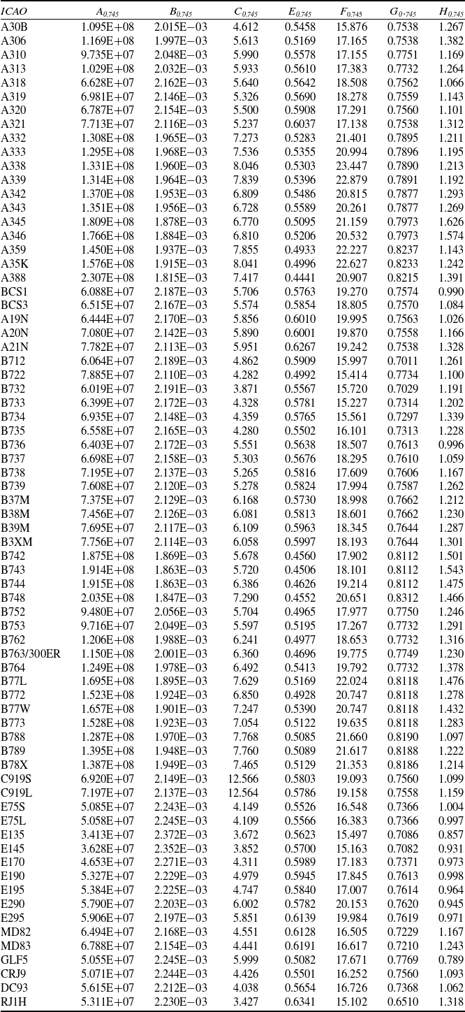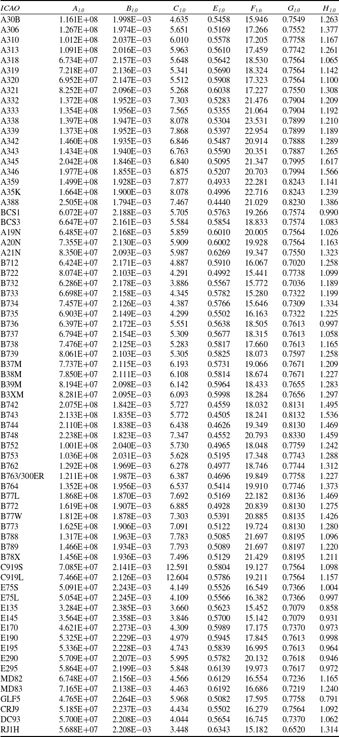As shown in Appendix A, when the design optimum conditions occur in the ISA troposphere, ( ${\varGamma}$ ) _DO is equal to −0.255, whilst in the ISA stratosphere, ( ${\varGamma}$ ) _DO is zero. Based upon this definition, an initial set of best estimates for the parameters necessary to obtain the design optimum conditions using Equations (24) to (27) for 67 aircraft was given in Table 2 of Poll and Schumann [Reference Poll and Schumann4]. This data set has now been updated and extended, with the corresponding coefficients for 71 aircraft being given in Table 1. The values presented in Table 1 supersede all previous versions.

Table 1.

Revised estimates of the P-S characteristic parameters for a range of aircraft

Table 1. Long description

Panel A: A table with columns labeled ICAO, (MTOM)ref, mdes, DO, (CF)DO 2, 1, 2, 3, 4, 5, 6. The table lists various aircraft models and their corresponding parameters. Panel B: A continuation of the table with additional aircraft models and their parameters. Panel C: Further continuation of the table with more aircraft models and their parameters.

In its current form, the P-S method is not valid for turboprop engines. This is because, as set out in detail in Poll and Schumann³, the P-S engine model relies upon very specific dimensional analysis arguments that are only valid for turbofan engines. Consequently, in the case of the turboprop, the variation of $\eta$ _o with C _T and M $ _{\infty} $ does not have the form shown in Figure 2, and the simple relation given in Equation (13) is not applicable. The basic physics of the turboprop is much more complicated, and further work needs to be done if the method is to be extended to cover this type of engine. However, whilst turboprop-powered aircraft currently account for 20% to 25% of the global fleet, since they operate exclusively on short-haul routes, they deliver only about 3% of the annual available seat kilometres flown globally. Consequently, in terms of the global annual fuel usage, turboprops are responsible for less than 3% of the total, whilst the turbofan aircraft in the current P-S data bank account for over 90%.

Table 2.

Coefficients A to H when $\iota $ _oo is equal to 0.75405

Table 2. Long description

A table comparing coefficients for various aircraft models. The table has 10 columns and 71 rows, including headers. The columns are labeled as ICAO, (MTOM)ref, mdes, DO, (CF)DO, 2, 1, 2, 3, 4, 5, and 6. Each row lists values for different aircraft models, such as A30B, A306, A310, and so on. The values include coefficients and other parameters relevant to the aircraft’s design and performance. Notable trends include variations in the coefficients and parameters across different aircraft models, reflecting their unique design characteristics and performance capabilities.

4.0 Operational optimum conditions

When either the aircraft mass is not equal to the design mass, or the variation of atmospheric temperature with pressure differs from the ISA, or both, as the FL is varied at a given flight Mach number, the maximum value of ( $\eta$ _o L/D) will not coincide with the local maxima for both $\eta$ _o and L/D. In this case, maximum ( $\eta$ _o L/D) is still given in Equations (8) and (9), but general solutions are difficult to find.

However, as described in Poll and Schumann [Reference Poll and Schumann4], the P-S method can be applied to any aircraft following a specified trajectory and the path dynamics yield the lift, drag and thrust at each Mach number and FL pair. Engine overall efficiency, $\eta$ _o , is then estimated from M $ _{\infty} $ and C _T , whilst L/D is estimated from M $ _{\infty} $ , C _L and C _d . Values of $\eta$ _o , C _T , C _L and C _d are then used in Equation (2) to obtain the instantaneous SAR. Since the method uses relations based upon established aerodynamic theory, rather than relying upon high-order polynomial curve fitting of performance data, differentiation with respect to any parameter continues to yield reasonably accurate results. Therefore, in principle, the operational optimum conditions can be obtained analytically. However, the nature of the relations is such that an analytic solution would be extremely complicated. Therefore, the approach adopted here is to use the P-S method to obtain numerical solutions of Equation (4) in the m, M $ _{\infty} $ and FL parameter space and use these to calibrate simple, approximate relations for the optimum conditions.

Calculations have been carried out for two aircraft – one a single-aisle and the other a twin-aisle configuration. Possible instantaneous masses range from the minimum value, taken to be operational empty mass (OEM), plus reserve fuel, to the certified MTOM. In practise, neither of these quantities is completely determined, since the OEM depends upon the cabin configuration and each aircraft type is usually produced with a variety of certified values of MTOM. However, examination of the aircraft database shows that achievable values of m typically lie within the range

(28) \begin{equation}0.8\left(m_{des}\right)\leq m\leq 1.2\left(m_{des}\right)\end{equation}

In addition, the properties of the atmosphere on any given day may vary markedly from the ISA values. For this study, at a given value of p $ _{\infty} $ , values of the temperature difference $\mathit{\Delta}$ T relative to the ISA have been taken to lie in the range

(29) \begin{equation}-20K\leq {\unicode{x0394}} T\leq +30K\end{equation}

With the temperature vertical lapse rate, L _h , lying in the range

(30) \begin{equation}-0.02 \ K/m\leq L_{h}\leq +0.02K/m\end{equation}

In Reference [Reference Poll and Schumann2], it was suggested that estimates of the operational optimum conditions could be obtained by applying Equations (24) to (27) and assuming that the coefficients $\psi $ ₁, $\psi $ ₂ and $\psi $ ₄ Footnote ⁶ were constant with their design optimum values, even though a weak Reynolds number dependence had been found. The numerical solutions show that this is a reasonable assumption for $\psi $ ₁, $\psi $ ₃ and $\psi $ _4, which exhibit less than ±1.5% over the parameter range considered. However, in the case of $\psi $ ₂ the variation is found to be much larger, being in the region of ±8%. Given the cost of fuel and the political sensitivity to carbon dioxide emissions, variations in fuel use of order 1% are deemed to be significant. Therefore, this simple approach is insufficiently accurate, and an improved estimation method is required.

In the new approach, the operational optimum ( $\eta$ _o L/D) is obtained by combining ( $\eta$ _o ) _OO from Equation (13) and (L/D) _OO , i.e.

(31) \begin{equation}\left(\eta _{o}L/D\right)_{\!OO}=\left(\eta _{o}\right)_{\!OO}\left(L/D\right)_{\!OO}\approx \eta _{1}\left(M_{OO}\right)^{{\eta _{2}}}\left(L/D\right)_{\!OO}\end{equation}

The other parameters depend only upon the airframe, and estimates are based upon the general form of Equations (25), (26) and (27), with the introduction of correction functionsFootnote ⁷ $f_{\textit{2}},\, f_{\textit{3}}$ and $f_{\textit{4}}$ , i.e.

(32) \begin{align} (C_{L})_{OO}=f_{2}\left(1-0.60b\left(1+{\varGamma} _{OO}\right)\right)\psi _{2}{\left({C}_{F}^{ac}\right)}_{OO}^{\left(\frac{1-\tau }{2}\right)} \\[-10pt] \nonumber\end{align}

(33) \begin{align} \left(L/D\right)_{\!OO}=f_{3}\left(1+0.08b\left(1+{\varGamma} _{OO}\right)\right)\psi _{3}{\left(\frac{1}{{C}_{F}^{ac}}\right)}_{\!OO}^{\!\left(\frac{1+\tau }{2}\right)} \\[10pt] \nonumber\end{align}

and

(34) \begin{equation}M_{OO}=f_{4}.\psi _{4}\end{equation}

where b is the constant coefficient in the skin friction relation given in Equation (21).

Experimentation with the numerical results reveals that, to a very good approximation, the f functions also have the general form

(35) \begin{equation}f\approx \frac{\left(1+\beta .b\left(1+{\varGamma} _{OO}\right)\right)}{\left(1+\beta .b\left(1+{\varGamma} _{DO}\right)\right)}\left(\frac{\left({C}_{F}^{ac}\right)_{\!OO}}{\big({C}_{F}^{ac}\big)_{DO}}\right)^{\!\delta }\end{equation}

where $\beta$ and $ \delta $ are constant coefficients, and f is equal to unity when conditions correspond to the design optimum values. Specifically, it is found that, for $f_{\textit{ 2}},\, f_{\textit{ 3}}$ and $f_{\textit{ 4}}$ , the corresponding values for $\beta$ and $ \delta $ are

(36) \begin{align} \beta _{2}\approx 0.542, \ \delta _{2}\approx -0.435 \\[-10pt] \nonumber\end{align}

(37) \begin{align} \beta _{3}\approx -0.062, \ \delta _{3}\approx 0.0450 \\[10pt] \nonumber \end{align}

and

(38) \begin{equation}\beta _{4}\approx -0.0645, \ \delta _{4}\approx -0.162\end{equation}

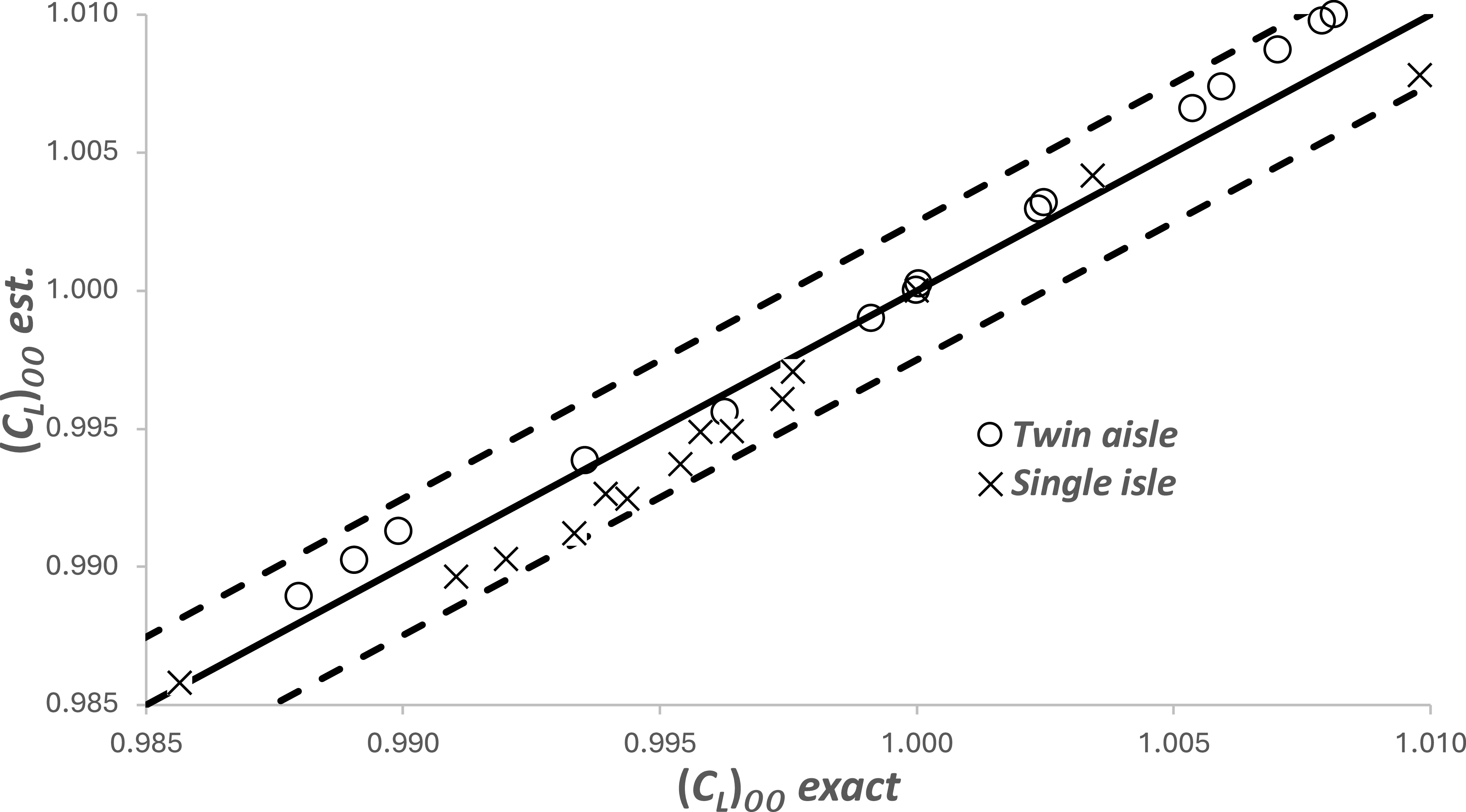
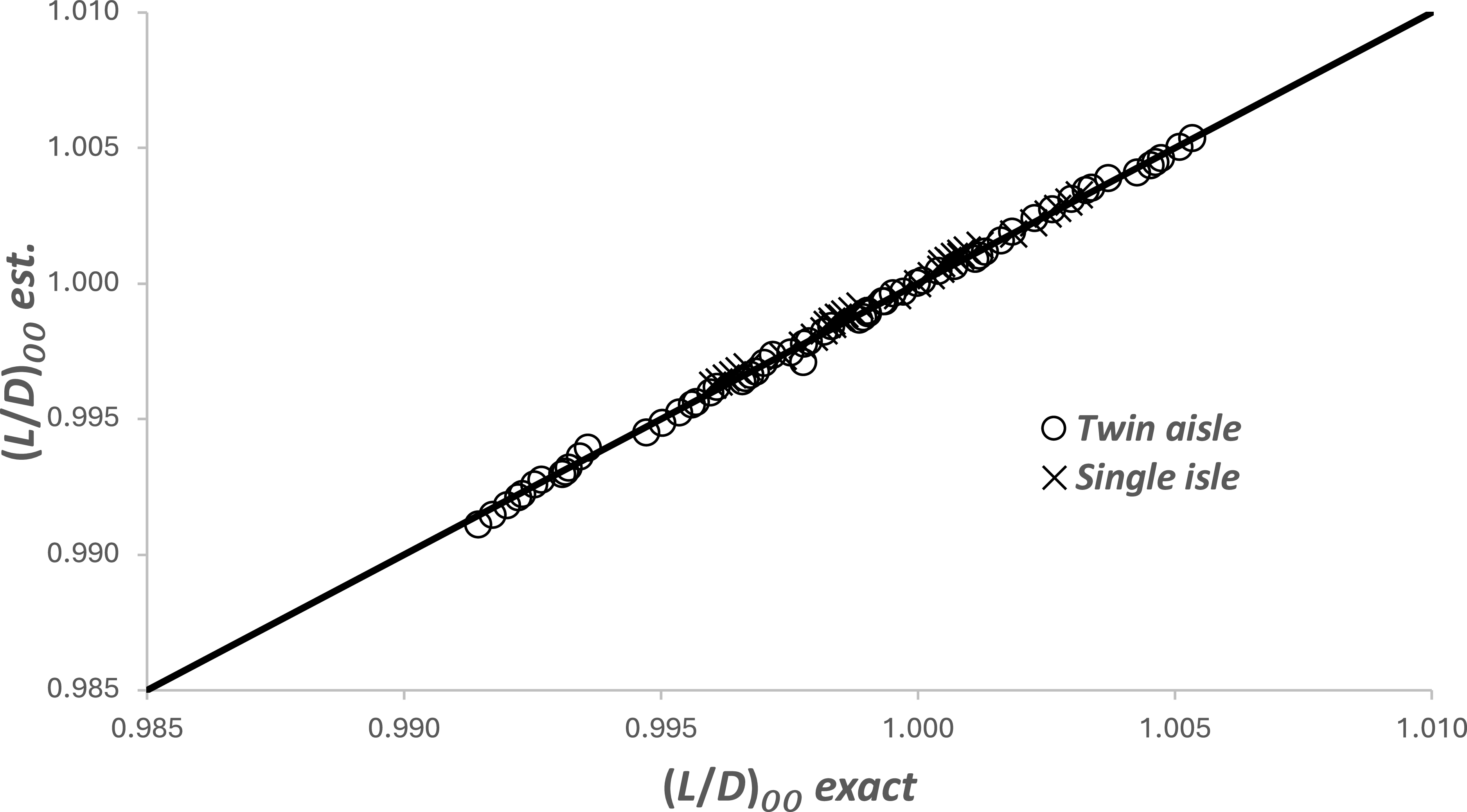
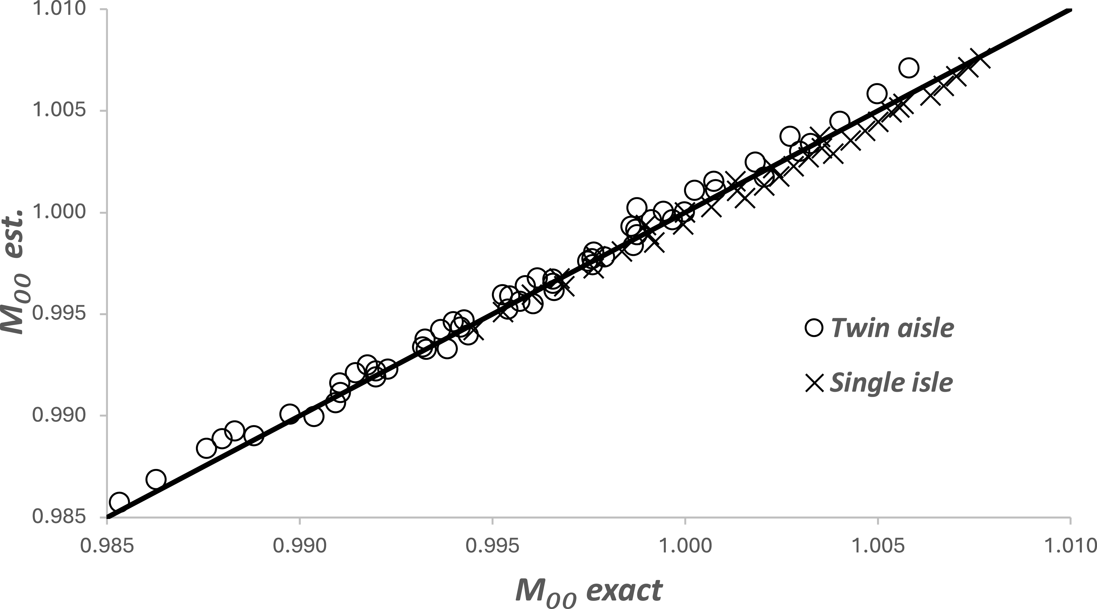
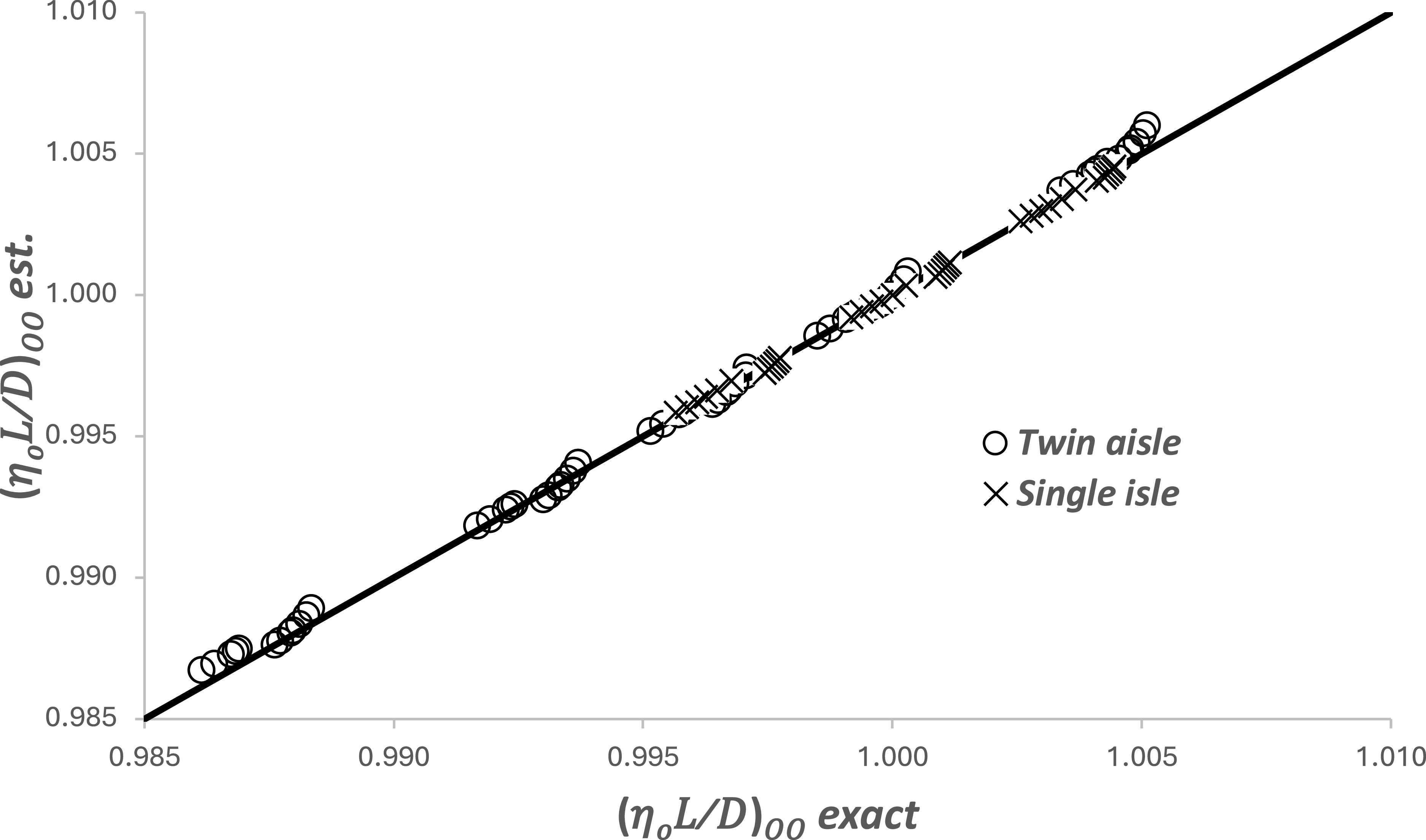
Comparisons between these approximations and the numerical values for both the large and the small aircraft are shown in Figures 3, 4, 5 and 6. Agreement is better than ±0.25% in all cases.

Figure 3.

Comparison between the estimated and the numerically exact values of the operational optimum lift coefficient for two aircraft types and a range of atmospheric conditions. The dashed lines show the ±0.25% deviation.

Figure 4.

Comparison between the estimated and the numerically exact values of the operational optimum lift-to-drag ratio for two aircraft types and a range of atmospheric conditions.

Figure 5.

Comparison between the estimated and the numerically exact values of the operational optimum Mach number for two aircraft types and a range of atmospheric conditions.

Figure 6.

Comparison between the estimated and the numerically exact values of the operational optimum range parameter for two aircraft types and a range of atmospheric conditions.

4.1 Basic relations

In the analysis that follows, it is assumed that the engine can provide the necessary thrust at all conditions. However, gas turbine engines have well-defined operating limits that are functions of atmospheric temperature. Therefore, when performing estimates for a particular engine-airframe combination, it is important to check that the engine can deliver the required thrust. Estimates for the various engine limits are given in Poll and Schumann [3, 4].

Substituting the results from Equations (36) to (38) into Equations (32), (33) and (34), taking b to be 0.14 and ignoring terms that are less than 0.001 in comparison to unity, gives

(39) \begin{align} {(C_{L})_{OO}\approx \left(1-0.021({\varGamma})_{OO}\right)\xi _{2}\left({C}_{F}^{ac}\right)}_{OO}^{\left(\frac{0.130-\tau }{2}\right)} \\[-10pt] \nonumber\end{align}

(40) \begin{align} \left(L/D\right)_{\!OO}\approx \left(1+0.002({\varGamma})_{OO}\right)\xi _{3}{\left(\frac{1}{{C}_{F}^{ac}}\right)}_{\!OO}^{\!\left(\frac{0.910+\tau }{2}\right)} \end{align}

(41) \begin{align} M_{OO}\approx \left(1-0.009({\varGamma})_{OO}\right){\xi _{4}\left(\frac{1}{{C}_{F}^{ac}}\right)}_{\!OO}^{\!0.162} \\[10pt] \nonumber\end{align}

and, from Equation (31),

(42) \begin{equation}\left(\eta _{o}L/D\right)_{\!OO} \approx \left(1-0.002\left(4.0\eta _{2}-1\right)({\varGamma})_{OO}\right)\xi _{1}{\left(\frac{1}{{C}_{F}^{ac}}\right)}_{OO}^{\left(\frac{0.910\left(1+0.36\eta _{2}\right)+\tau }{2}\right)}\end{equation}

where

(43) \begin{align} \xi _{1}\approx \left(\eta _{1}{\xi }_{4}^{\eta _{2}}\right)\xi _{3} &=\left(\frac{1.011}{1-0.009\left(1+\eta _{2}\right)({\varGamma})_{DO}}\right){\psi _{1}\left({C}_{F}^{ac}\right)}_{DO}^{0.162\left(\eta _{2}-0.28\right)} \\[-10pt] \nonumber\end{align}

(44) \begin{align} \xi _{2} & \approx \left(\frac{0.916}{1+0.0705({\varGamma})_{DO}}\right){\psi _{2}\left({C}_{F}^{ac}\right)}_{DO}^{0.435} \\[-10pt] \nonumber\end{align}

(45) \begin{align} \xi _{3} & \approx \left(\frac{1.011}{1-0.009({\varGamma})_{DO}}\right){\psi _{3}\left(\frac{1}{{C}_{F}^{ac}}\right)}_{DO}^{0.045} \\[10pt] \nonumber\end{align}

and

(46) \begin{equation}\xi _{4}\approx \left(\frac{1}{1-0.009({\varGamma})_{DO}}\right)\psi _{4}{\left({C}_{F}^{ac}\right)}_{DO}^{0.162}\end{equation}

The $\xi $ parameters only depend upon the design conditions and, consequently, are characteristics of the aircraft and engine combination. Values are included in Table 1.

4.2 Reynolds number

As shown in Appendix A, the operational optimum value for the Reynolds number is given by

(47) \begin{equation}\left(R^{ac}\right)_{\!OO}={S}_{ref}^{1/2}\left(\frac{\gamma p_{\infty }M_{\infty }}{\mu _{\infty }a_{\infty }}\right)_{\!OO}\approx {S}_{ref}^{1/2}\left(\frac{\gamma p_{TP}}{\mu _{TP}a_{TP}}\right)_{\!ISA}\left(\frac{(\, p_{\infty})_{OO}}{\left(\, p_{TP}\right)_{ISA}}\right)^{{\!\iota _{OO}}}\left(\frac{M_{OO}}{1+1.34(\overline{{\unicode{x0394}} T})}\right)\end{equation}

where $\iota $ _OO is equal to 0.74505 if p $ _{\infty} $ is greater than, or equal to, (p _TP ) _ISA ; otherwise, $\iota $ _OO is equal to 1. The change in the value of $\iota $ _OO is necessary because the atmospheric temperature at a given pressure is measured relative to the ISA, and the ISA has a discontinuity in lapse rate when p $ _{\infty} $ is equal to (p _TP ) _ISA .

Using the definition of lift coefficient given in Equation (5), the Reynolds number may be expressed as

(48) \begin{equation}\left(R^{ac}\right)_{\!OO}\approx \left(\frac{\psi _{5}}{1+1.34(\overline{{\unicode{x0394}} T})_{OO}}\right){\left(\frac{\psi _{4}}{M_{OO}}\right)^{\!\left(2\iota _{OO}-1\right)}}\left(\frac{\psi _{6}}{(C_{L})_{OO}}\left(\frac{m}{MTOM_{ref}}\right)\right)^{{\!\iota _{OO}}}\end{equation}

where

(49) \begin{equation}\psi _{5}={S}_{ref}^{1/2}\left(\frac{\gamma p_{TP}}{\mu _{TP}a_{TP}}\right)_{\!ISA}\end{equation}

and

(50) \begin{equation}\psi _{6}=\frac{MTOM_{ref}.g}{\left(\gamma /2\right)\left(\, p_{TP}\right)_{ISA}{\psi }_{4}^{2}S_{ref}}\end{equation}

The lift coefficient and Mach number are now eliminated by the use of Equations (41) and (43) leading to

(51) \begin{equation}\left(R^{ac}\right)_{\!OO}\approx \left(\frac{\psi _{5} \ }{1+1.34(\overline{{\unicode{x0394}} T})_{OO}-0.020({\varGamma})_{OO}}\right)\bigg(\frac{\psi _{4}}{\xi _{4}}\bigg)^{0.4901}\left(\frac{\psi _{6}}{\xi _{2}}\left(\frac{m}{MTOM_{ref}}\right)\right)^{\!0.74505}{\left({C}_{F}^{ac}\right)}_{OO}^{\left(\frac{\tau +0.083}{2.684}\right)}\end{equation}

when $\iota $ _OO is equal to 0.74505 and

(52) \begin{equation}\left(R^{ac}\right)_{\!OO}\approx \left(\frac{\psi _{5}}{1+1.34(\overline{{\unicode{x0394}} T})_{OO}-0.030({\varGamma})_{OO}}\right)\left(\frac{\psi _{4}}{\xi _{4}}\right)\left(\frac{\psi _{6}}{\xi _{2}}\left(\frac{m}{MTOM_{ref}}\right)\right){\left({C}_{F}^{ac}\right)}_{OO}^{\left(\frac{\tau +0.194}{2}\right)}\end{equation}

when $\iota $ _OO is equal to unity.

From Equation (21),

(53) \begin{equation}\left({C}_{F}^{ac}\right)_{\!OO}\approx \frac{0.0269}{{\left(R^{ac}\right)}_{OO}^{0.14}}\end{equation}

Hence, when $\iota $ _OO is 0.74505,

(54) \begin{equation}\left(R^{ac}\right)_{\!OO}\approx A_{0.745}\left(\left(\frac{1}{1+1.34(\overline{{\unicode{x0394}} T})_{OO}-0.020({\varGamma})_{OO}}\right)\left(\frac{m}{MTOM_{ref}}\right)^{0.74505}\right)^{\!\left(\frac{0.996}{1+0.05\tau }\right)}\end{equation}

where

(55) \begin{equation}A_{0.74505}=\left(0.0269\right)^{0.371\left(\frac{\tau +0.083}{1+0.05\tau }\right)}\left(\psi _{5}{\left(\frac{\psi _{4}}{\xi _{4}}\right)^{0.4901}}\left(\frac{\psi _{6}}{\xi _{2}}\right)^{0.74505}\right)^{\!\left(\frac{0.996}{1+0.05\tau }\right)}\end{equation}

and when $\iota $ _OO is unity,

(56) \begin{equation}\left(R^{ac}\right)_{\!OO}\approx A_{1}\left(\left(\frac{ \ 1}{1+1.34(\overline{{\unicode{x0394}} T})_{OO}-0.030({\varGamma})_{OO}}\right)\left(\frac{m}{MTOM_{ref}}\right)\right)^{\!\left(\frac{0.987}{1+0.07\tau }\right)}\end{equation}

where

(57) \begin{equation}A_{1}\approx \left(0.0269\right)^{0.493\left(\frac{\tau +0.194}{1+0.07\tau }\right)}\left(\psi _{5}\left(\frac{\psi _{4}}{\xi _{4}}\right)\left(\frac{\psi _{6}}{\xi _{2}}\right)\right)^{\!\left(\frac{0.987}{1+0.07\tau }\right)}\end{equation}

The A values are included in Table 1.

As shown in Table 1, $\tau$ always lies in the range 0.1–0.2. Hence, without significant loss of accuracy, Equations (54) and (56) may be further simplified to

(58) \begin{equation}\left(R^{ac}\right)_{\!OO}\approx \left(\frac{A_{0.745}}{1+1.32(\overline{{\unicode{x0394}} T})_{OO}-0.020({\varGamma})_{OO}}\right)\left(\frac{m}{MTOM_{ref}}\right)^{\!0.736}\end{equation}

and

(59) \begin{equation}\left(R^{ac}\right)_{\!OO}\approx \left(\frac{A_{1}}{1+1.31(\overline{{\unicode{x0394}} T})_{OO}-0.030({\varGamma})_{OO}}\right)\left(\frac{m}{MTOM_{ref}}\right)^{\!0.976}\end{equation}

It follows that the value of aircraft mass, m _T , for which R ^ac is the same for both values of $\iota $ _oo is

(60) \begin{equation}\left(\frac{m_{T}}{MTOM_{ref}}\right)\approx \left(1-0.06(\overline{{\unicode{x0394}} T})_{OO}-0.039({\varGamma})_{OO}\right)\left(\frac{A_{0.745}}{A_{1}}\right)^{\!4.16}\end{equation}

This is the mass for which the optimum operational cruise FL is 360.89, and it is seen to be a weak function of the atmospheric parameters, with maximum likely deviations being of the order 1%.

Equation (60) is valid when $\mathit{\Delta}$ T and ${\varGamma}$ are continuous functions of p _∞, and this is the most likely situation in real atmospheres. However, in theoretical studies, the operational atmosphere is often taken to be an ISA + $\mathit{\Delta}$ T where $\mathit{\Delta}$ T is constant. In this case, ${\varGamma}$ is discontinuous when p $ _{\infty} $ is equal to (p _TP ) _ISA, and it is easily shown that

(61) \begin{equation}\left(\frac{m_{T}}{MTOM_{ref}}\right)\approx 0.979\left(1-0.02(\overline{{\unicode{x0394}} T})_{OO}\right)\left(\frac{A_{0.745}}{A_{1}}\right)^{\!4.16}\end{equation}

If m is greater than or equal to m _T , $\iota $ _oo is equal to 0.75405 and, if m is less than m _T , $\iota $ _oo is equal to unity. Therefore, depending upon the value of $\iota $ _oo , either Equation (58) or Equation (59) gives the Reynolds number at the optimum condition in terms of aircraft mass, m, the characteristics of the atmosphere, $\mathit{\Delta}$ T and ${\varGamma}$ and fixed characteristics of the aircraft, $\xi $ ₂ , $\xi $ ₄ , $\psi $ _4, $\psi $ ₅ , $\psi $ ₆ and $\tau$ .

4.3 Skin friction coefficient

With the operational optimum Reynolds number determined, the mean skin-friction coefficient follows from Equations (53), (58) and (59), i.e.

(62) \begin{equation}\left({C}_{F}^{ac}\right)_{\!OO}\approx B_{0.745}\left(1+0.19(\overline{{\unicode{x0394}} T})_{OO}-0.003({\varGamma})_{OO}\right)\left(\frac{MTOM_{ref}}{m}\right)^{\!0.103}\end{equation}

and

(63) \begin{equation}\left({C}_{F}^{ac}\right)_{\!OO}\approx B_{1}\left(1+0.18(\overline{{\unicode{x0394}} T})_{OO}-0.004({\varGamma})_{OO}\right)\left(\frac{MTOM_{ref}}{m}\right)^{\!0.137}\end{equation}

where B is

(64) \begin{align}B=\frac{0.0269}{A^{0.14}} \\[-20pt] \nonumber \end{align}

4.4 Range parameter ( $\eta$ _o L/D)

The operational optimum value of ( $\eta$ _o L/D) is obtained from Equations (42), (62) and (63). Again, neglecting terms that are less than 0.001 in comparison to unity, this becomes

(65) \begin{equation}\left(\eta _{o}L/D\right)_{\!OO}\approx C_{0.745}(1-0.11(\overline{{\unicode{x0394}} T})_{OO})\left(\frac{m}{MTOM_{ref}}\right)^{\!\left(\frac{0.910\left(1+0.36\eta _{2}\right)+\tau }{19.41}\right)}\end{equation}

and

(66) \begin{equation}\left(\eta _{o}L/D\right)_{\!OO}\approx C_{1}(1-0.11(\overline{{\unicode{x0394}} T})_{OO})\left(\frac{m}{MTOM_{ref}}\right)^{\!\left(\frac{0.910\left(1+0.36\eta _{2}\right)+\tau }{14.63}\right)}\end{equation}

where

(67) \begin{align}C={\xi _{1}}\left(\frac{1}{B}\right)^{\!\left(\frac{0.910\left(1+0.36\eta _{2}\right)+\tau }{2}\right)} \\[-20pt] \nonumber \end{align}

4.5 Lift coefficient

The operational optimum lift coefficient comes from Equations (39), (62) and (63), i.e.

(68) \begin{equation}(C_{L})_{OO}\approx E_{0.745}\left(1-0.021({\varGamma})_{OO}\right)\left(\frac{m}{MTOM_{ref}}\right)^{\!\left(\frac{\tau -0.130}{19.41}\right)}\end{equation}

and

(69) \begin{equation}(C_{L})_{OO}\approx E_{1}\left(1-0.021({\varGamma})_{OO}\right)\left(\frac{m}{MTOM_{ref}}\right)^{\!\left(\frac{\tau -0.130}{14.63}\right)}\end{equation}

where

(70) \begin{align}E={\xi _{2}}\left(B\right)^{\left(\frac{0.130-\tau }{2}\right)} \\[-20pt] \nonumber \end{align}

4.6 Lift-to-drag ratio

The operational optimum lift-to-drag ratio comes from Equations (40), (62) and (63), i.e.

(71) \begin{equation}\left(L/D\right)_{\!OO}\approx F_{0.745}\left(1-0.10(\overline{{\unicode{x0394}} T})_{OO}+0.004({\varGamma})_{OO}\right)\left(\frac{m}{MTOM_{ref}}\right)^{\!\left(\frac{0.910+\tau }{19.41}\right)}\end{equation}

and

(72) \begin{equation}\left(L/D\right)_{\!OO}\approx F_{1}\left(1-0.10(\overline{{\unicode{x0394}} T})_{OO}+0.004({\varGamma})_{OO}\right)\left(\frac{m}{MTOM_{ref}}\right)^{\!\left(\frac{0.910+\tau }{14.63}\right)}\end{equation}

where

(73) \begin{align}F={\xi _{3}}\left(\frac{1}{B}\right)^{\!\left(\frac{0.910+\tau }{2}\right)}\\[-20pt] \nonumber \end{align}

4.7 Mach number

The operational optimum Mach number comes from Equations (41), (62) and (63), i.e.

(74) \begin{equation}M_{OO}\approx G_{0.745}(1-0.03(\overline{{\unicode{x0394}} T})_{OO}-0.009({\varGamma})_{OO})\left(\frac{m}{MTOM_{ref}}\right)^{\!0.017}\end{equation}

and

(75) \begin{equation}M_{OO}\approx G_{1}(1-0.03(\overline{{\unicode{x0394}} T})_{OO}-0.008({\varGamma})_{OO})\left(\frac{m}{MTOM_{ref}}\right)^{\!0.022}\end{equation}

where

(76) \begin{align}G={\xi _{4}}\left(\frac{1}{B}\right)^{\!0.162} \\[-20pt]\nonumber \end{align}

4.8 Flight level

From the definition of lift coefficient and using Equation (50)

(77) \begin{align}(C_{L})_{OO}=\frac{m.g}{\frac{\gamma }{2} \ {(\, p_{\infty})_{OO}}{M}_{OO}^{\!2}S_{ref}} \ =\psi _{6}\left(\frac{\left(\, p_{TP}\right)_{ISA}}{(\, p_{\infty})_{OO}}\right)\left(\frac{\psi _{4}}{M_{OO}}\right)^{2}\left(\frac{m}{(MTOM)_{ref}}\right) \ \end{align}

Hence, the static pressure at the optimum operational altitude is

(78) \begin{align}\frac{(\, p_{\infty})_{OO}}{\left(\, p_{TP}\right)_{ISA}} \ =\left(\frac{\psi _{6}}{(C_{L})_{OO}}\right)\left(\frac{\psi _{4}}{M_{OO}}\right)^{\!2}\left(\frac{m}{(MTOM)_{ref}}\right) \ \end{align}

Once again, the evaluation of (C _L ) _OO and M _OO requires the specification of $\iota $ , and this is obtained by comparing m with m _T from Equation (60), or Equation (61). As already noted, if m is greater than or equal to m _T , $\iota $ _oo is equal to 0.75405 and, using Equations (68) and (74),

(79) \begin{align}\frac{(\, p_{\infty})_{OO}}{\left(\, p_{TP}\right)_{ISA}}\approx H_{0.745}\left(1+0.06(\overline{{\unicode{x0394}} T})_{OO}+0.039({\varGamma})_{OO}\right)\left(\frac{m}{(MTOM)_{ref}}\right)^{\!\left(\frac{18.89-\tau }{19.41}\right)}\end{align}

whilst, if m is less than m _T , $\iota $ _oo is equal to unity and, from Equations (69) and (75),

(80) \begin{align}\frac{(\, p_{\infty})_{OO}}{\left(\, p_{TP}\right)_{ISA}}\approx H_{1}(1+0.06(\overline{{\unicode{x0394}} T})_{OO}+0.038({\varGamma})_{OO})\left(\frac{m}{(MTOM)_{ref}}\right)^{\!\left(\frac{14.11-\tau }{14.63}\right)}\end{align}

where

(81) \begin{equation}H=\left(\frac{\psi _{6}}{E}\right)\left(\frac{\psi _{4}}{G}\right)^{\!2}\end{equation}

Using the relations given in Poll and Schumann [1], local static pressure is linked directly to the FL and, if (p $ _{\infty} $ ) _OO is greater than (p _TP ) _ISA ,

(82) \begin{equation}FL_{OO}=1454.42\left(1-0.751865\left(\frac{(\, p_{\infty})_{OO}}{\left(\, p_{TP}\right)_{ISA}}\right)^{\!0.190263}\right)\end{equation}

otherwise

(83) \begin{equation}FL_{OO}=360.892\left(1-0.576511ln\left(\frac{(\, p_{\infty})_{OO}}{\left(\, p_{TP}\right)_{ISA}}\right)\right)\end{equation}

4.9 True airspeed

From the definition of Mach number, the true airspeed, V _OO , is given by

(84) \begin{equation}V_{OO}=M_{OO}\sqrt{\left(\gamma \mathfrak{R}T_{OO}\right)}=M_{OO}\sqrt{\left(\gamma \mathfrak{R}(T_{TP})_{ISA}\right)}{\left(\left(\frac{T}{T_{TP}}\right)_{ISA}+\overline{{\unicode{x0394}} T}\right)}_{\!OO}^{\!\frac{1}{2}}\end{equation}

From Reference [1], if FL _OO is less than or equal to 360.892,

(85) \begin{equation}\left(\frac{T}{T_{TP}}\right)_{ISA}=1.3300-0.0009144\left(FL_{oo}\right)\end{equation}

and, if FL _OO is greater than 360.892,

(86) \begin{equation}\left(\frac{T}{T_{TP}}\right)_{ISA}=1.0\end{equation}

Values of the coefficients A to G when $\iota $ _oo is equal to 0.75405 are given in Table 2 and values A to G when $\iota $ _oo is equal to 1 are given in Table 3.

Table 3.

Coefficients A to H when $\iota $ _oo is equal to1

Table 3. Long description

Panel A: Table listing coefficients A to H for various aircraft models when oo is equal to 1. The table includes columns for ICAO codes and coefficients A to H. Panel B: Table listing coefficients A to G for various aircraft models when oo is equal to 0.75405. The table includes columns for ICAO codes and coefficients A to G.

Figure 7.

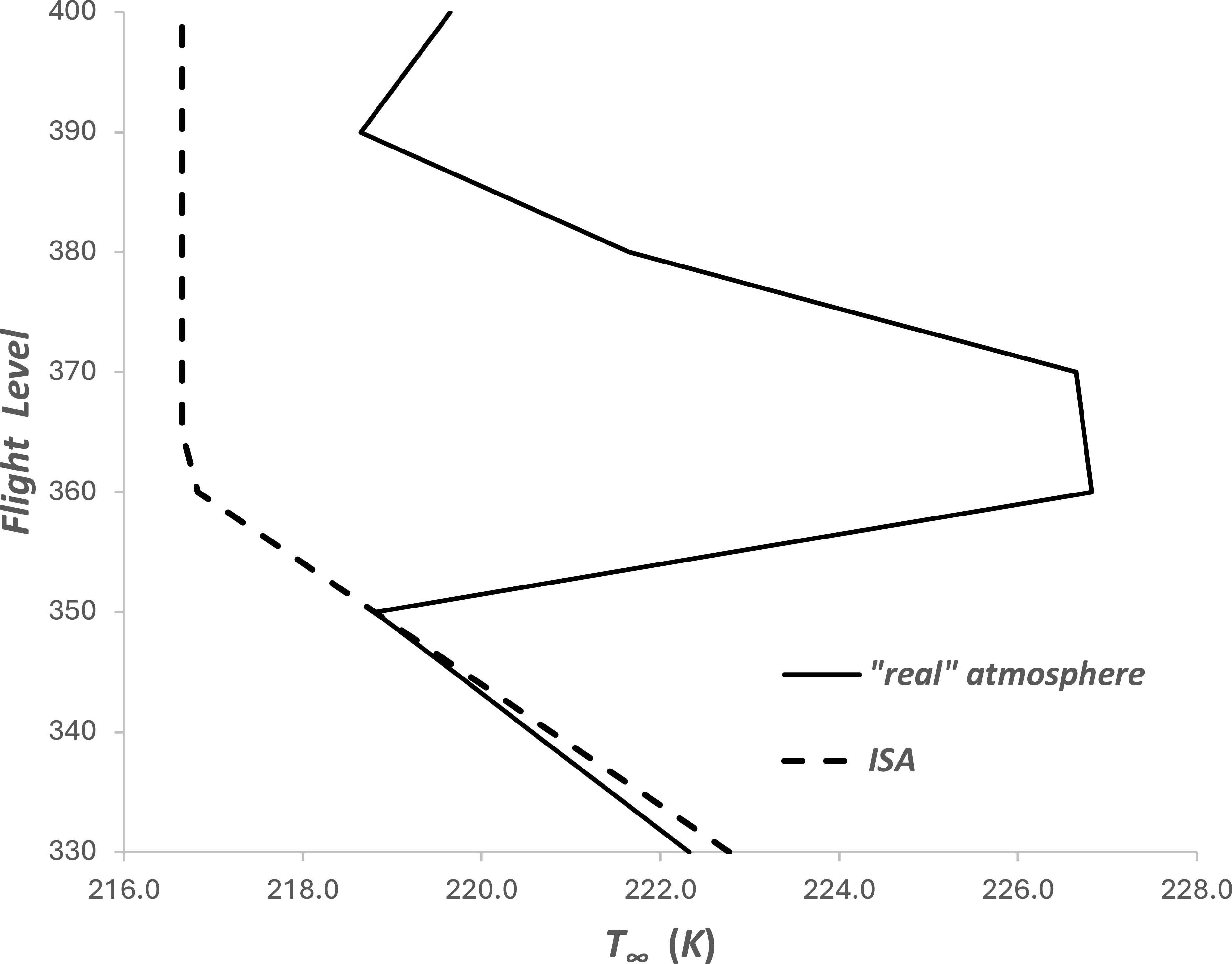
An example of an observed variation of atmospheric temperature with FL compared with that in the ISA. Figure taken from Poll and Schumann [Reference Poll and Schumann9].

5.0 Sample calculation

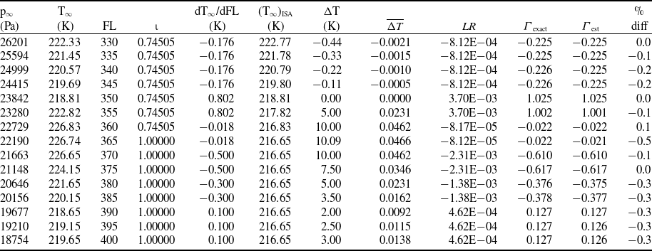
An example of an observed variation of atmospheric temperature with pressure obtained by a weather balloon, originally used in Poll and Schumann [Reference Poll and Schumann9], is given in Figure 7 together with the variation in the ISA. Clearly, whilst the variation of temperature with pressure (FL) in the ISA is monotonically decreasing, this is not the case in the example of the real atmosphere shown. The corresponding variations of $\mathit{\Delta}$ T and ${\varGamma}$ are given in Table 4. In this case, the deviations in static temperature are quite small. However, the deviations in lapse rate are very large and include changes in sign.

Table 4.

An example of an observed variation of atmospheric temperature with pressure and the processing steps to estimate steps ${\varGamma}$ , Poll and Schumann [Reference Poll and Schumann9]

Table 4. Long description

A table with 19 rows and 10 columns. The columns are labeled as Pa, T, FL, T ISA, T %, LR exact, LR est, LR diff, and FL. The table presents data on atmospheric temperature variations with pressure and the processing steps to estimate steps. Each row provides specific values for each column, detailing the observed variations and deviations in static temperature and lapse rate.

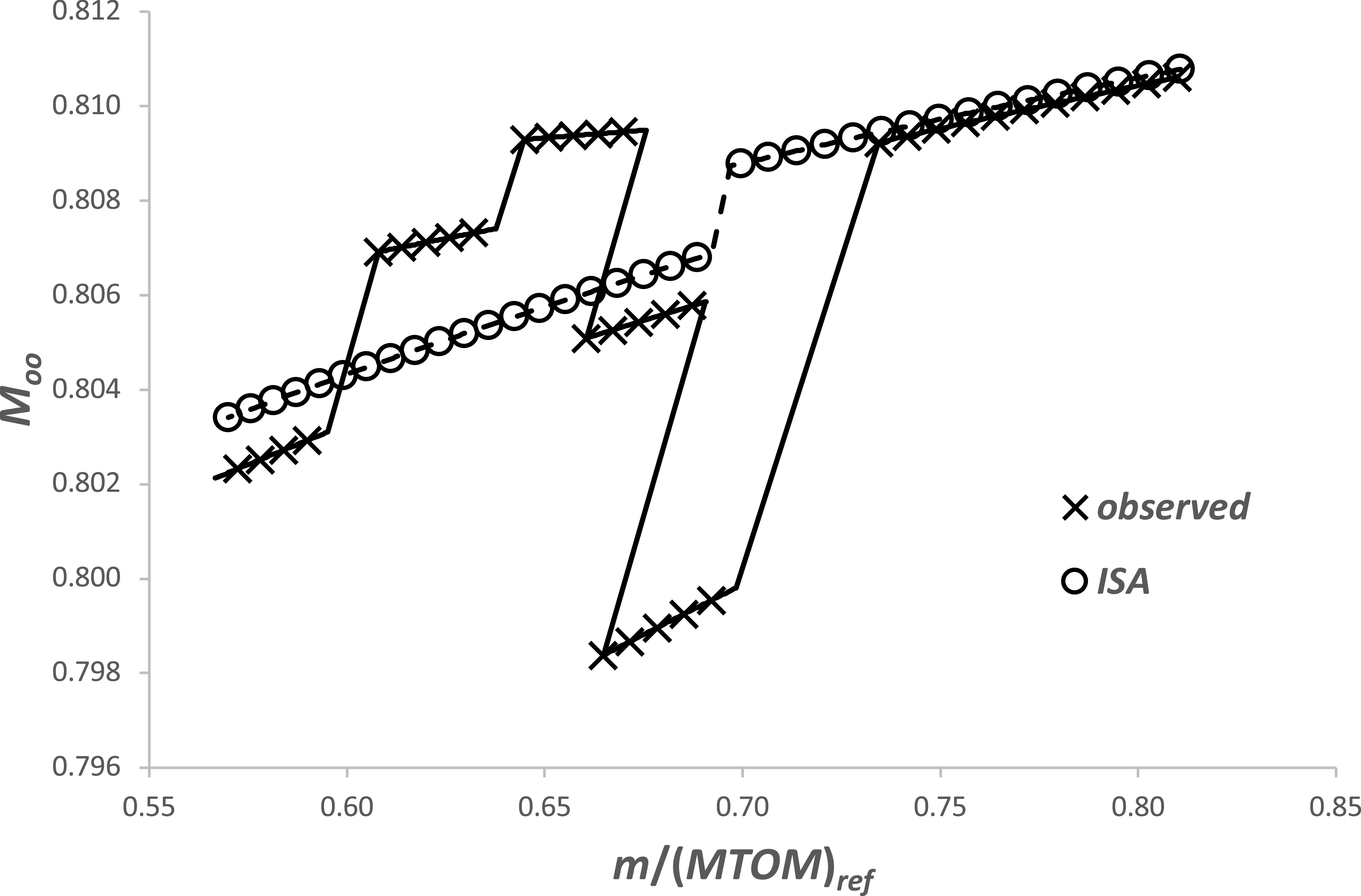
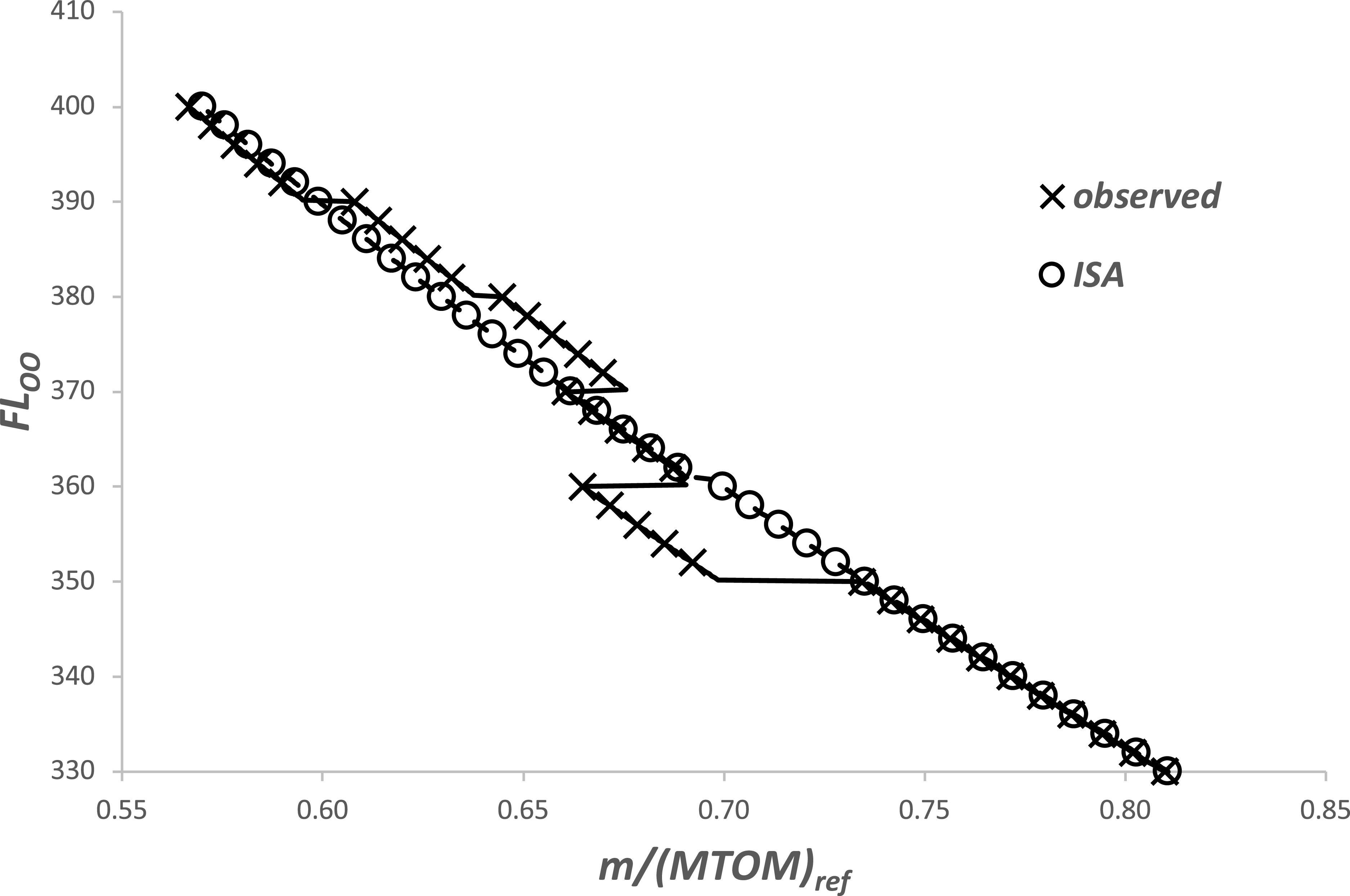
Using the twin-aisle aircraft, the variations of optimum Mach number, FL and ( $\eta$ _o L/D) with aircraft mass are given in Figures 8, 9 and 10. Results are presented for both the observed temperature distribution and the ISA.

The difference between M _OO with aircraft mass for the two atmospheres is small, with a maximum of about 1%, but not insignificant in operational terms. However, the important thing to notice is that, whilst the relationship is mostly single-valued, from a mass ratio between 0.675 and 0.690, it is double-valued, and between 0.665 and 0.675, it is triple-valued.

In the case of FL _OO , the general trend of increasing FL with decreasing aircraft mass is found. Between the two atmospheres FL differences of up to 10 points, or about 1000 feet, are found and, again, there are double and triple values. These differences, whilst not large, are still operationally significant, particularly in the context of contrail avoidance by changes in altitude.

Figure 10 shows that the variation of the range parameter with mass is also operationally significant, with a change of about 3%. In this example, the impact of atmospheric variation is also significant, with maximum differences being in the region of 1%.

Figure 8.

The variation of the optimum operational FL with aircraft mass for a twin-aisle aircraft.

Figure 9.

The variation of the optimum operational FL with aircraft mass for a twin-aisle aircraft.

6.0 Improved range equation

The example given in the previous section shows how ( $\eta$ _o L/D) varies with both aircraft mass, m, and the atmospheric characteristics. This can now be used to estimate the amount of fuel required to cruise a given distance.

Figure 10.

The variation of the optimum operational range parameter with aircraft mass for a twin-aisle aircraft.

The relationship between fuel used and distance travelled through the air in straight and level flight is obtained by rearranging Equation (3) and integrating to give

(87) \begin{equation}{\int }_{\!\!S_{1}}^{S_{2}}dS=\left(\frac{LCV}{g}\right){\int }_{\!\!m_{2}}^{m_{1}}\frac{\left(\eta _{O}L/D\right)}{m}dm\end{equation}

where m ₁ and m ₂ are the values of aircraft mass at S ₁ and S ₂ . The difference between m ₁ and m ₂ is the total fuel used, m _f .

However, wind and temperature data are given in terms of position relative to the ground. Therefore, if there is a tailwind component, $V_{w}$ , the relationship between S and the distance travelled over the ground, S _G , is

(88) \begin{equation}{\int }_{\!\!S_{1}}^{S_{2}}dS={\int }_{\!\!0}^{R_{G}}\frac{dS_{G}}{\left(1+\frac{V_{w}}{V_{\infty }}\right)}=R_{G}-{\int }_{\!\!0}^{R_{G}}\frac{V_{w}}{\left({V_{\infty }}+V_{w}\right)}d{S_{G}}={R_{G}}-({\unicode{x0394}} R_{G})_{w}\end{equation}

where R _G is the total ground distance travelled. In general, the wind speed and the true airspeed are functions of both position relative to the ground and altitude. As shown in Sections 4.8 and 4.9, the operational optimum values of FL and V $ _{\infty} $ depend upon the aircraft mass, which, in turn, depends upon the fuel usage. This means that the evaluation of these integrals will usually require iteration.

If the range parameter, ( $\eta$ _o L/D), is taken to be constant, the fuel required for a given ground distance is

(89) \begin{equation}\frac{m_{f}}{m_{1}}=1-EXP\left(-\frac{\left(R_{G}-({\unicode{x0394}} R_{G})_{w}\right).g}{\left(\eta _{O}L/D\right)LCV}\right)\end{equation}

This is a version of the well-known Breguet range equation inverted to give mission fuel as a function of range (see, for example, Torenbeek [Reference Torenbeek5], Martinez-Val et al. [Reference Martinez-Val, Palacin and Perez6] and Randle et al. [Reference Randle, Hall and Vera-Morales7]).

However, as shown in Section 2.5, the range parameter is a function of the aircraft mass, with the general form being

(90) \begin{equation}\left(\eta _{o}L/D\right)_{\!OO}\propto \left(\frac{m}{MTOM_{ref}}\right)^{\epsilon }\end{equation}

and, as shown in Section 2.5, if m is greater than, or equal to, m _T (Equation (60), or (61)), $\varepsilon$ is equal to 0.063 ± 0.0025 (Equation 65) and if m is less than m _T , $\varepsilon$ is equal to 0.083 ± 0.0035 (Equation (66)).

Hence, from Equation (87), if m is always greater than m _T ,

(91) \begin{equation}{\int }_{\!\!S_{1}}^{S_{2}}\frac{dS}{(1-0.11(\overline{{\unicode{x0394}} T})_{OO})}=15.87\left(\frac{\left(\eta _{O}L/D\right)_{{m_{1}}}.LCV}{g\big(1-0.11{(\overline{{\unicode{x0394}} T})}_{OO}^{S_{1}}\big)}\right)\left(1-\left(\frac{m_{2}}{m_{1}}\right)^{0.063}\right)\end{equation}

Now, using the results in Equation (88),

(92) \begin{equation}{\int }_{\!\!S_{1}}^{S_{2}}\frac{dS}{(1-0.11(\overline{{\unicode{x0394}} T})_{OO})}\approx {\int }_{\!\!0}^{R_{G}}\frac{V_{\infty }\left(1+0.11(\overline{{\unicode{x0394}} T})_{OO}\right)}{\left({V_{\infty }}+V_{w}\right)}dS_{G} \ =R_{G}-({\unicode{x0394}} R_{G})_{w}+({\unicode{x0394}} R_{G})_{{\unicode{x0394}} T} \ \end{equation}

where

(93) \begin{equation}({\unicode{x0394}} R_{G})_{{\unicode{x0394}} T}\approx 0.11{\int }_{\!\!0}^{R_{G}}\frac{V_{\infty }(\overline{{\unicode{x0394}} T})_{OO}}{\left({V_{\infty }}+V_{w}\right)}dS_{G}\end{equation}

In general, and to maintain ( $\eta$ _o L/D) at its optimum value, the aircraft will be changing altitude as S _G as increases. Consequently, this term involves changes in tailwind and temperature in both the horizontal and vertical planes. Therefore, as with ( $\mathit{\Delta}$ R _G ) _W , evaluation of ( $\mathit{\Delta}$ R _G ) $_{\mathit{\Delta}T}$ will require iteration.

The corresponding fuel requirement is

(94) \begin{equation}\frac{m_{f}}{m_{1}}=1-\left(1-0.063\left(\frac{g\big(1-0.11{(\overline{{\unicode{x0394}} T})}_{OO}^{S_{1}}\big)}{\left(\eta _{O}L/D\right)_{{m_{1}}}LCV}\left(R_{G}-({\unicode{x0394}} R_{G})_{w}+({\unicode{x0394}} R_{G})_{{\unicode{x0394}} T}\right)\right)\right)^{\!15.87}\end{equation}

Similarly, if m is always less than m _T ,

(95) \begin{equation}\frac{m_{f}}{m_{1}}=1-\left(1-0.083\left(\frac{g\big(1-0.11{(\overline{{\unicode{x0394}} T})}_{OO}^{S_{1}}\big)}{\left(\eta _{O}L/D\right)_{{m_{1}}}LCV}\left(R_{G}-({\unicode{x0394}} R_{G})_{w}+({\unicode{x0394}} R_{G})_{{\unicode{x0394}} T}\right)\right)\right)^{\!12.05}\end{equation}

In the special case where m ₂ is equal to m _T , the ground distance covered is

(96) \begin{equation}\left(R_{G}-({\unicode{x0394}} R_{G})_{w}+({\unicode{x0394}} R_{G})_{{\unicode{x0394}} T}\right)_{T}=\left(R_{G}\right)_{T}- \ {\int }_{0}^{\left(R_{G}\right)_{T}}\frac{V_{w}}{\left({V_{\infty }}+V_{w}\right)}dS_{G}+0.11{\int }_{0}^{\left(R_{G}\right)_{T}}\frac{V_{\infty }(\overline{{\unicode{x0394}} T})_{OO}}{\left({V_{\infty }}+V_{w}\right)}dS_{G}\end{equation}

and

(97) \begin{equation}\left(R_{G}\right)_{T}\approx 15.87\left(\frac{\left(\frac{\eta _{O}L}{D}\right)_{{m_{1}}}.\,LCV}{g\big(1-0.11{(\overline{{\unicode{x0394}} T})}_{OO}^{S_{1}}\big)}\right)\left(1-\left(\frac{m_{T}}{m_{1}}\right)^{0.063}\right)+\left(({\unicode{x0394}} R_{G})_{w}-({\unicode{x0394}} R_{G})_{{\unicode{x0394}} T}\right)_{T} \ \end{equation}

whilst the fuel used is

(98) \begin{equation}\frac{(m_{f})_{T}}{m_{1}}=1-\frac{m_{T}}{m_{1}}\end{equation}

Hence, if m ₁ is greater than m _T and m ₂ is less than m _T , the fuel requirement is

(99) \begin{equation}\frac{m_{f}}{m_{T}}=1-\frac{m_{T}}{m_{1}}\left(1-0.083\left(\frac{g\left(1-0.11{(\overline{{\unicode{x0394}} T})}_{OO}^{\left(R_{G}\right)_{T}}\right)}{\left(\eta _{O}L/D\right)_{{m_{T}}}LCV}\left(R_{G}-\left(R_{G}\right)_{T}-{\left[({\unicode{x0394}} R_{G})_{w}-({\unicode{x0394}} R_{G})_{{\unicode{x0394}} T}\right]}_{\left(R_{G}\right)_{T}}^{R_{G}}\right)\right)\right)^{\!12.05}\end{equation}

7.0 Discussion

Although the foregoing analysis may appear to be complex, the results given in Sections 4.2 to 4.9 are both simple and easy to use. The operational optimum range parameter, ( $\eta$ _o L/D) _OO , is found to have a clear dependency upon aircraft mass, increasing as the mass increases. For take-off masses ranging from the minimum likely to the maximum possible, the difference is about 5%. This is large enough to affect the trip fuel requirement for long-haul flights where weight loss due to fuel may be up to 25% of the take-off value. Deviations in atmospheric static temperature from the ISA values also have a noticeable effect, with ( $\eta$ _o L/D) decreasing as $\mathit{\Delta}$ T increases, again, changes of the order±1% are possible. However, variations in the vertical temperature lapse rate (LR) are found to be negligible.

The optimum value of lift coefficient is a very weak function of mass and is independent of $\mathit{\Delta}$ T. However, it does depend upon LR, with changes of ±2% being possible. In addition, the optimum Mach number, which was assumed to be constant in previous work, is found to exhibit a weak dependence upon m, $\mathit{\Delta}$ T and LR. In all cases, the maximum likely variation is of order±1%. The optimum FL depends upon the optimum values of both lift coefficient and Mach number. Whilst the FL is driven primarily by aircraft mass, increases in $\mathit{\Delta}$ T can reduce the optimum FL by about 2 units (≈200 feet), whilst increases in LR can reduce it by 8 units (≈800 feet).

The results obtained in this analysis are both qualitatively and quantitatively similar to those presented in the original papers by Poll and Schumann [Reference Poll and Schumann9, Reference Poll and Schumann10]. In this case, a much simpler model, proposed by Poll [Reference Poll8], was used to represent the aircraft and engine combination. This was based upon the hypothesis that, when suitably normalised, the variation of ( $\eta$ _o L/D) with Mach number and lift coefficient was approximately the same for all aircraft. The results of the present study provide evidence in support of that very simple hypothesis.

Figure 11.

A comparison between the improved range equations and the Breguet version for ISA conditions and zero wind with total distance flown.

Regarding the extended range equation, Figure 11 gives the results from Equations (94) and (95) compared with those from the Breguet equation, Equation (89), for zero wind and ISA conditions. In this particular case, the impact of varying aircraft mass as fuel is consumed is shown, and the non-dimensional ground distance flown is

(100) \begin{equation}X=\frac{g.R_{G}}{\left(\eta _{O}L/D\right)_{{m_{1}}}LCV}\end{equation}

The upper limit of X equal to 0.6 corresponds to a range of about 20,000 kms, or half the circumference of the Earth. A trip from London to Johannesburg is about 10,000 kms, i.e. an X of about 0.3, whilst London to New York is about 5,000 kms, or an X of approximately 0.15. The classic Breguet equation always gives a lower value of (m _f /m ₁ ) for a given X and, whilst these differences are not large, being around 1% for long-haul flights. This is equivalent to about 1,000 kgs of fuel. It is also important to note that assuming ( $\eta$ _o L/D) to be fixed at its initial value locks out the effect of en-route temperature variations, and these may also change the fuel requirement by a similar amount.

Finally, in the example described in Section 5.0, it was found that, for some values of mass, there were multiple solutions for the optimum FL and Mach number. This is because, unlike the ISA, the variation of temperature with pressure is not a monotonically decreasing (or increasing) function. Specifically, referring to Figures 8 and 9, for masses in the range 0.665–0.675, there are three solutions for FL _OO ranging from 360 to 375, i.e. a 4% change. Similarly, there are three values of M _OO ranging from 0.798 (FL _OO = 360) to 0.810 (FL _OO = 360), i.e. 1.5%. However, as shown in Figure 10, the range parameter and, hence, the SAR is essentially constant. Therefore, in this example, the operator would have a choice of three different FLs for the same SAR and with Mach numbers differing only by about 1%. This has important implications for planning flights that avoid contrails by flying above, or below, regions of the atmosphere where the air is super-saturated with respect to ice.

Any desk-based study for flight in the ISA would find a single solution for the operating conditions at each aircraft mass. Consequently, moving away from the optimum FL to avoid an ISSR would necessarily incur a small fuel penalty. However, as shown above, this is not a conclusion that is valid for all atmospheric conditions; rather, it is a specific result valid only for the idealised ISA.

8.0 Conclusions

Previous work has been extended to provide rapid and accurate estimates of the optimum operational SAR for an aircraft of given total mass in a completely general atmosphere. Simple relationships have also been found for the corresponding values of lift coefficient, Mach number and FL. The variation of optimum operational SAR with mass is significant, and it increases as the aircraft mass increases. In addition, there is a small reduction in SAR as the air temperature increases above the ISA value for the same FL. Taking these influences into account, an improved and complete range equation, including the effects of wind and temperature variations in both the horizontal and vertical wind planes, has been presented. Depending upon the distance flown and the atmospheric conditions en route, the trip fuel requirement may vary by several percent relative to the estimates from the traditional Breguet formulation.

The FL for optimum SAR is found to depend upon both the local temperature deviation from ISA and the vertical temperature lapse rate. Sample calculations using an observed temperature profile show that, in regions where the sign of the lapse rate is changing, there can be more than one solution for the FL for optimum SAR for a given aircraft mass. The possibility that very nearly the same value of SAR may be achieved at more than one FL has implications for fuel usage when exercising contrail avoidance by vertical deviation. Currently, there is a widely held belief that any (temporary) deviation in cruise altitude from an aircraft’s flight-plan value must lead to an increase in fuel consumption. This may be true for operation in the idealised ISA. However, since changes in SAR with height in the real atmosphere may differ significantly in magnitude and may be of opposite sign to those occurring in the ISA, when avoiding contrails, it may be possible to move to different altitudes at which the SAR is essentially the same as the undisturbed, flight-plan value and, possibly, even less. To ensure continuous operation at optimum, or near optimum, conditions, accurate temperature and temperature gradient data are required all along the route and in real time.

Airlines operate their aircraft using a cost index, which is the ratio of the cost of time to the cost of fuel for a flight. Conditions for optimum SAR correspond to operation at a cost index of zero. This method provides a baseline for future work exploring the implications of operating at a non-zero cost index.