

NOMENCLATURE
- a
-
non-linear stiffness exponent
- A
-
harmonic balancing matrix
- ah
-
non-dimensional displacement from mid-chord to elastic axis
- b
-
semi-chord
- c
-
chord length
- C
-
structural damping matrix
- d
-
observational data
- D
-
harmonic balance operator
- E
-
harmonic balance transformation matrix
- F
-
force matrix
- K
-
structural stiffness matrix
- M
-
structural mass matrix
- NH
-
number of harmonics
- q
-
modal deflections
- Q
-
harmonic balance solution vector
- r α
-
radius of gyration about elastic axis
- wi
-
Wagner variables
- x
-
spatial displacement
- x α
-
non-dimensional distance from elastic axis to centre of mass
- α
-
pitch amplitude
- β
-
cubic stiffness coefficient
- η i
-
term from rational approximation of generalised aerodynamic forces, i = 1, . . ., nl
- θ
-
random event
- λ
-
Newton-Raphson relaxation parameter
- μ
-
mass ratio
- ξ
-
non-dimensional plunge displacement
- Φ
-
truncated matrix of eigenvectors
- ω
-
fundamental solution frequency
-
 $\bar{\omega }$
-
frequency ratio,
$\bar{\omega }={\frac{\omega _{\xi }}{\omega _{\alpha }}}$
Greek Symbol


1.0 INTRODUCTION
As simulation tools are created for problems of higher complexity, it becomes increasingly difficult for practitioners to be confident that their model accurately replicates the physical behaviour of the phenomena of interest. Even if an adequate physical description of the system is implemented, ensuring all parameters and coefficients that drive the simulation are accurately defined can be problematic. This adversely affects the calibration and validation processes during the development of the simulation tool. Various dynamic aeroelastic phenomena provide good examples of complex physical behaviour, which are dependent on many parameters that are rife with variability and are difficult to ascertain. Due to the highly variable nature of both the structural and flow characteristics, Pettit has identified the need for consideration of parametric uncertainty in the prediction of aeroelastic stability(Reference Pettit1). This uncertainty is epistemic in nature and arises from a lack of understanding about subtle characteristics of the structural body and local flow conditions. Subsequently, research has been carried out to investigate how parametric uncertainty influences the aeroelastic behaviour of the aircraft.
Marques et al investigated the impact of structural variability on transonic flutter predictions for a range of models and illustrated the high sensitivity of aeroelastic stability(Reference Marques, Badcock, Khodaparast and Mottershead2,Reference Marques, Badcock, Khodaparast and Mottershead3) . Limit-Cycle Oscillations (LCOs) are also a pertinent issue for some in-service aircraft due to their non-linear nature; hence, they carry considerable practical interest(Reference Bunton and Denegri4,Reference Thomas, Dowell, Hall and Denegri5) . As for flutter, LCOs are sensitive to parametric variability and have been investigated using various uncertainty propagation techniques(Reference Beran, Pettit and Millman6-Reference Hayes and Marques9). Despite the many studies conducted to examine the consequences of parametric uncertainty, there have been few attempts to characterise this uncertainty for aeroelastic problems. By using experimental data of output quantities, e.g. LCO amplitudes from flight tests, to accurately calibrate models, stochastic analysis of aeroelastic phenomena can be carried out with a higher degree of confidence.
Bayesian inference is a technique tailored for using external observations to reduce epistemic uncertainty. The Bayesian framework is applicable to the calibration of complex and expensive computer models and identification of input parameters(Reference Kennedy and O’Hagan10). It has become more widely recognised in recent years as a useful statistical paradigm; many publications describe the concept and its applications(Reference Tanner11-Reference Congdon13). In Bayesian inference, all quantities are random variables; hence, the outcome of the analysis will be a probability distribution. This permits the use of any resulting parameter probability densities to be directly propagated through the model for further uncertainty quantification analyses(Reference Smith14). The prior distribution regularises the problem and means the probabilities that are calculated can be meaningful for small amounts of experimental data(Reference Fellin, Lessmann, Oberguggenberger and Vieider15). Furthermore, Bayesian statistics allow the successive addition of more observations by making the posterior distribution the new prior. This is useful from a practical perspective, particularly in model updating.
These methods have been applied to structural variability identification(Reference Dwight, Haddad-Khodaparast and Mottershead16) and the calibration of constants in turbulence models with promising results(Reference Oliver and Moser17,Reference Edeling, Cinnella, Dwight and Bijl18) . Dwight et al reduced uncertainty in the predictions of flutter speeds based on epistemic variability on numerous structural parameters(Reference Dwight, Bijl, Marques and Badcock19). However, there is a lack of documentation for non-linear aeroelastic implementations of Bayesian inference. The work presented here focuses on implementing a Bayesian inference strategy driven by a Markov-chain Monte Carlo (MCMC) algorithm to estimate model parameters, which ultimately will improve model performance in the case of non-linear aeroelasticity. First, a HDHB formulation is exploited to determine the LCO conditions without incurring the high costs of time-accurate simulations. Then, the practicality of using the HDHB approach to drive the MCMC algorithm for parameter estimation is investigated. The paper will first describe the Bayesian inference and MCMC strategies, followed by the implementation of the HDHB formulation. Finally, results from the model calibration of three cases will be presented and discussed: a 2 Degrees of Freedom (DoF) aerofoil with unknown damping and non-linear stiffness, a Goland wing with the equivalent unknown parameters, and the same wing with unknown store Centre of Gravity (CG) location and trailing-edge spar thickness.
2.0 BAYESIAN INFERENCE
Bayesian inference updates the probability that the model will provide accurate predictions based on observations and uses Bayes’ rule to compute the posterior probability distributions:
 $$\begin{equation}
P(\theta |d) \propto P(d|\theta )P_{0}(\theta ),
\end{equation}$$
where θ represents deterministic parameter values from the set of all possible values, Θ. These parameters influence a particular quantity of interest, observations of which are denoted by d. P 0(θ) is the prior, which describes the perceived distribution of input parameters that allow the model to perform well before any observations are made. The prior provides an opportunity for the the user to impart any knowledge about the uncertain parameters into the analysis and enables highly accurate parameter estimations with scarce data resources. The likelihood, P(d|θ), measures the probability of observing a particular quantity of interest value, d, given the inputs, θ. The posterior is given as P(θ|d); this is the perceived probability distribution of the input parameters once the observed evidence has been accounted for. This translates to how likely the model is to provide accurate predictions for a given set of input parameters.
For the uncertainties of the input parameters to be updated, first the model needs to be related to the observational data using a statistical model. In this work, the statistical model described by Kennedy and O’Hagan(Reference Kennedy and O’Hagan10) is employed:
 $$\begin{equation}
d=m(\theta )+\epsilon \sim \mathcal {N} (0,{\sigma _{\epsilon }}^{2}),
\end{equation}$$
where m(θ) is the model output for a particular deterministic input parameter set, θ. This statistical model represents the error between the model and experimental data as noise, ε, which is described by a normal distribution with mean 0 and standard deviation σε. From inspection of the posterior probability distribution, a deterministic value of θ can be found, which gives the most accurate model predictions based on the observed evidence. For the statistical model described in Equation (2), the likelihood is expressed as:
 $$\begin{equation}
P(d|\theta )^{n}=\exp \left({-\frac{1}{2}\sum ^{k}_{i=1}{\frac{(d(i)-m(i,\theta ))^{2}}{{\sigma _{\epsilon }}^{2}}}}\right),
\end{equation}$$
where n is the MCMC iteration number, k denotes the number of experimental data points used in the analysis, and i refers to a known input parameter shared between the data and model, i.e. velocity in this work. To obtain the posterior distribution, MCMC is used and is described below.
MCMC
MCMC is a random walk method used to sample from a known probability density function. More specifically, the approach taken here is known as the Metropolis-Hastings algorithm, a commonly used form of MCMC(Reference Hastings20). A concise description of the fundamental idea of this technique is given below. The posterior is calculated proportionately using one and drives the MCMC through a set of selection criteria. These rules for accepting samples maximise the posterior in a probabilistic sense and are given as:
 $$\begin{equation}
\left\{\begin{array}{l@{\qquad}l}
{\displaystyle\frac{{P(\theta|d)}^{n}}{{P(\theta|d)}^{n-1}}} \geq 1,\ \mathrm{accept\ with\ probability\ of}\ 1 \nonumber\\[11pt] {\displaystyle\frac{{P(\theta|d)}^{n}}{{P(\theta|d)}^{n-1}}} < 1,\ \mathrm{accept\ with\ probability\ of}\ {\frac{P(\theta|d)^{n}}{P(\theta|d)^{n-1}}} \nonumber\\
\end{array}\right.
\end{equation}$$
New samples are randomly selected from a multivariate Gaussian distribution, which is centred about the current sample location. The covariance of this proposal distribution is user-defined. Optimal convergence occurs when the proposal distribution matches the shape and size of the posterior. The chain will walk randomly around the parameter space, moving to the regions of high posterior value with a high sample acceptance rate and occasionally to regions of low posterior value. It can be shown under mild conditions on the proposal distribution that the resulting chain samples the posterior(Reference Metropolis, Rosenbluth, Rosenbluth, Teller and Teller21). As a result, the final posterior distribution will represent a stochastic set of parameter values, which allow the model to perform best across all situations contained within the experimental data.
Frequently, the initial parameter values chosen to start the MCMC chain lie in a region of low probability thus contaminating the random walk result. To eliminate this form of error, a burn-in phase is defined. This specifies a number of samples to be discarded from the start of the chain. If a sufficient number of MCMC samples and burn-in phase sizes are defined, a statistically accurate sampling of the posterior results.
3.0 HDHB
The HDHB formulation used in this work was proposed by Hall et al(Reference Hall, Thomas and Clark22) for time-periodic flow problems; this methodology was adapted to non-linear dynamical systems by Liu et al(Reference Liu, Thomas, Dowell, Attar and Hall23) and is summarised next. Consider a dynamic system with a non-linearity in stiffness whose behaviour can be described using a simple equation of motion given by:
 $$\begin{equation}
{\bf M} \ddot{x} + {\bf C} \dot{x}+ {\bf K} x + {\bf K}_{nl}(x)= {\bf F}(x,\dot{x},\ddot{x},t)
\end{equation}$$
Matrices
 $\bf M$
,
 $\bf C$
and
 $\bf K$
describe the mass, damping and linear stiffness properties of the system, respectively, and K
nl
(x) is the non-linear component of the stiffness restoring force. The external force, F can be a function of the motion of the system and time. Here, we consider the external force to be F = sin (ωt). The solution of Equation (5) can be approximated by a truncated Fourier series of NH
harmonics with a fundamental frequency ω.
 $$\begin{equation}
x(t)\approx \hat{x}_{0}+\sum _{n=1}^{N_{H}} (\hat{x}_{2n-1}\cos (n\omega t)+\hat{x}_{2n}\sin (n\omega t))
\end{equation}$$
The first and second derivatives of x(t) with respect to time can be found to be:
 $$\begin{equation}
\dot{x}(t)& \approx& \sum _{n=1}^{N_{H}} (-n\omega \hat{x}_{2n-1}\sin (n\omega t)+n\omega \hat{x}_{2n}\cos (n\omega t)),\\
\end{equation}$$
 $$\begin{equation}
\ddot{x}(t)& \approx& \sum _{n=1}^{N_{H}} (-{(n\omega )}^{2}\hat{x}_{2n-1}\cos (n\omega t) -{(n\omega )}^{2}\hat{x}_{2n}\sin (n\omega t))
\end{equation}$$
 $$\begin{equation}
({\bf M}\omega ^{2}{\bf A}^{2}+{\bf C}\omega {\bf A} + {\bf K}{\bf I}){\hat{\bf Q}}+{\hat{\bf Q}}_{nl}-{\bf F} {\hat{\bf H}}=0,
\end{equation}$$
where
 $$\begin{equation*}
\hat{\bf Q}= \left\lbrace \begin{array}{c}\hat{x}_{0} \\
\hat{x}_{1} \\
\hat{x}_{2} \\
\hat{x}_{3} \\
\vdots \\
\hat{x}_{2N_{H}} \end{array} \right\rbrace _{2N_{H}+1},\ {\hat{\bf Q}}_{nl}= \left\lbrace \begin{array}{c}\hat{K_{nl}}_{0} \\
\hat{K_{nl}}_{1} \\
\hat{K_{nl}}_{2} \\
\hat{K_{nl}}_{3} \\
\vdots \\
\hat{K_{nl}}_{2N_{H}} \end{array} \right\rbrace _{2N_{H}+1}\mathrm{\ and\ } \hat{\bf H}= \left\lbrace \begin{array}{c}0 \\
0 \\
1 \\
0 \\
\vdots \\
0 \end{array} \right\rbrace _{2N_{H}+1}.
\end{equation*}$$
Matrix A reconstructs the Fourier series from the harmonic balance and is shown in the work of Hayes and Marques(Reference Hayes and Marques9). The non-linear term Fourier coefficients,
 $\hat{{\bf Q}}_{nl}$
are computed using Discrete Fourier Transforms (DFT). Computing these terms analytically can be cumbersome for certain types of non-linearities such as high-order polynomial terms or fluxes in computational fluid dynamics problems(Reference Hall, Thomas and Clark22). The HDHB method overcomes these issues by casting the problem in the time domain where the Fourier coefficients are related to 2NH
+ 1 equally spaced sub-time levels throughout one temporal period using a constant transformation matrix, which yields:
 $$\begin{equation}
{\hat{\bf Q}} ={\bf E} {\tilde{\bf Q}},\ {\hat{\bf Q}}_{nl} ={\bf E} {\tilde{\bf Q}}_{nl} \mathrm{ \ and \ } {\hat{\bf H}} = {\bf E}{\tilde{\bf H}},
\end{equation}$$
where:
 $$\begin{equation*}
\tilde{\bf Q}= \left\lbrace \begin{array}{c}x(t_{0}) \\
x(t_{1}) \\
\vdots \\
x(t_{2N_{H}}) \end{array} \right\rbrace ,\ {\tilde{\bf Q}}_{nl}= \left\lbrace \begin{array}{c}K_{nl}(x(t_{0})) \\
K_{nl}(x(t_{1})) \\
\vdots \\
K_{nl}(x(t_{2N_{H}})) \end{array} \right\rbrace \mathrm{\ and\ } \tilde{\bf H}= \left\lbrace \begin{array}{c}\sin t_{0}\\
\sin t_{1}\\
\vdots \\
\sin t_{2N_{H}} \end{array} \right\rbrace
\end{equation*}$$
and
 $$\begin{equation}
t_{i}={\frac{i2\pi }{2N_{H}+1}}\ (i=0,1,\ldots ,2N_{H})
\end{equation}$$
Expressions for the transformation matrix
 $\bf E$
and its inverse E
−1, which can be used to relate the time domain variables back to the Fourier coefficients, i.e.
 $\tilde{\bf Q}={\bf {E}}^{-1} \hat{\bf Q}$
, are shown in the work of Hayes and Marques(Reference Hayes and Marques9). Using these transformation matrices, Equation (9) can be cast in the time domain as:
 $$\begin{equation}
({\bf M}\omega ^{2}{\bf D}^{2}+{\bf C}\omega {\bf D} + {\bf K}{\bf I}){\tilde{\bf Q}} + {\tilde{\bf Q}}_{nl} - {\bf F}{\tilde{\bf H}}=0={\bf R,}
\end{equation}$$
where D = E −1 AE. Equation (12) represents the HDHB system and can be solved using either pseudo-time marching or Newton-Raphson approaches. Here, the latter is employed to benefit from its fast convergence rates:
 $$\begin{equation}
{\bf S}^{n+1}={\bf S}^{n}-\lambda {\bf J}^{-1}{\bf R}^{n},
\end{equation}$$
where S n is the solution vector at iteration n and λ is a relaxation parameter for increased stability. The inverse Jacobian of the system, J −1, is numerically approximated using finite-differences(Reference Thomas, Dowell and Hall24) and R n is the residual of Equation (12) at iteration n, i.e.
 $$\begin{equation*}
{\bf S}^{n}= \left\lbrace \begin{array}{c}\hat{x}_{0} \\
{\hat{x}}_{1} \\
\vdots \\
{\hat{x}}_{2N_{H}} \end{array} \right\rbrace ^{n},\ {\bf R}^{n}= \left\lbrace \begin{array}{c}R_{0} \\
R_{1} \\
\vdots \\
R_{2N_{H}} \end{array} \right\rbrace ^{n}\mathrm{\ and\ }\ {\bf J}= \left[ \begin{array}{c@{\quad}c@{\quad}c}\frac{\partial {R_{0}}}{\partial {\hat{x}}_{0}} & \dots & {\frac{\partial R_{0}}{\partial {\hat{x}}_{2N_{H}}}}\\
\vdots &\ddots &\vdots \\
{\frac{\partial R_{2N_{H}}}{\partial {\hat{x}}_{0}}}&\dots &{\frac{\partial R_{2N_{H}}}{\partial {\hat{x}}_{2N_{H}}}} \end{array} \right]
\end{equation*}$$
4.0 PITCH-PLUNGE AEROFOIL
The equations of motion for a pitch/plunge aerofoil with non-linear restoring forces have been presented by Lee et al(Reference Lee, Liu and Chung25). They can be displayed in the form of Equation (5) where the terms are given as:
 $$\begin{equation*}
{\bf M}= \left[ \begin{array}{c@{\quad}c}x_{\alpha }&{1} \\
[0.4cm]{1}&{\frac{x_{\alpha }}{r^2_{\alpha }}} \end{array} \right],\ {\bf C}= \left[ \begin{array}{c@{\quad}c}0&{\frac{2\zeta _{\xi }\overline{\omega }}{V^*}} \\
{ \frac{2\zeta _{\alpha }}{V^*}\dot{\alpha }}&{0} \end{array} \right],\ {\bf K}= \left[ \begin{array}{c@{\quad}c}0&{\frac{k_{\xi }{\overline{\omega }}^{2}}{{V^*}^{2}}} \\
[-0.1cm]{\frac{k_{\alpha }}{{V^*}^{2}}}&{0} \end{array} \right],
\end{equation*}$$
 $$\begin{equation*}
x=\left\lbrace \begin{array}{c}\alpha \\
[0.6cm]{\xi } \end{array} \right\rbrace ,\ {\bf K}_{nl}= \left[\hphantom{\hspace{-2.84544pt}} \begin{array}{c@{\quad}c}0&{\frac{\beta _{\xi }{\overline{\omega }}^{2}}{{V^*}^{2}}} \\
[0.3cm]{\frac{\beta _{\alpha }}{{V^*}^{2}}}&{0} \end{array} \hphantom{\hspace{-2.84544pt}}\right] \left\lbrace \begin{array}{c}\alpha ^{3} \\
[0.6cm]{\xi ^{3}} \end{array} \hphantom{\hspace{-5.69046pt}}\right\rbrace ,\ {\bf F}= \left\lbrace \hphantom{\hspace{-2.84544pt}} \begin{array}{c}-\frac{C_L(\tau )}{\pi \mu }+ \frac{bP(\tau )}{mV^2} \\
[0.3cm]{\frac{2C_M(\tau )}{\pi \mu r^2_{\alpha }} + \frac{Q(\tau )}{m V^2 r^2_{\alpha }}} \end{array} \hphantom{\hspace{-2.84544pt}}\right\rbrace ,
\end{equation*}$$
where ξ is the non-dimensional plunge displacement of the elastic axis and α is the pitch. CL
and Cm
correspond to the lift and pitching moment coefficients, respectively, and P(τ) and Q(τ) are external forces and moments, respectively. After the introduction of four new variables, w
1, w
2, w
3, w
4, which partially describe the aerodynamic and external forces characterised by
 $\bf F$
, the equations of motion and generalised aerodynamic terms can be written as:
 $$\begin{equation}
\left\{\begin{array}{l@{\qquad}l}
{c}_{0}{\xi}^{\prime\prime}+{c}_{1}{\alpha}^{\prime\prime}+{c}_{2}{\xi}^{\prime}
+{c}_{3}{\alpha}^{\prime}
+{c}_{4}{\xi}+{c}_{5_{\beta}}{\xi}^{3}+{c}_{6}{\alpha}+{c}_{7}{w}_{1}+{c}_{8}{w}_{2}
+{c}_{9}{w}_{3}+{c}_{10}{w}_{4}=f({t^{*}}) \nonumber\\ {d}_{0}{\xi}^{\prime\prime}+{d}_{1}{\alpha}^{\prime\prime}+{d}_{2}{\alpha}^{\prime}
+{d}_{3}{\alpha} +{d}_{4_{\beta}}{\alpha}^{3}+{d}_{5}{\xi}^{\prime}+
{d}_{6}{\xi}+{d}_{7}{w}_{1}+{d}_{8}{w}_{ 2}
+{d}_{9}{w}_{3}+{d}_{10}{w}_{4}=g({t^{*}})
\vspace{0.01cm} \nonumber\\
w^{\prime}_{1}=\alpha-\epsilon_{1}w_{1}\nonumber\\
w^{\prime}_{2}=\alpha-\epsilon_{2}w_{2} \nonumber\\
w^{\prime}_{3}=\alpha-\epsilon_{1}w_{3} \nonumber\\
w^{\prime}_{4}=\alpha-\epsilon_{2}w_{4}
\label{system1a}\end{array}\right.,
\end{equation}$$
where f(t*) and g(t*) represent the remainder of the generalised aerodynamic forces and damp out with time, and hence, are not part of the periodic solution. The non-linearity is only considered in the pitch DoF so βξ = 0. Expressions for the remainder of the coefficients of Equation (14) can be found in the work of Lee et al(Reference Lee, Gong and Wong26). Implementing the HDHB approach to Equation (14) yields a system in the frequency domain.
 $$\begin{equation}
\left\{\begin{array}{l@{\qquad}l}
(c_{0}{\omega}^{2}{\bf A}^{2}+c_{2}{\omega}{\bf A}+c_{4}{\bf I}){\hat {\bf Q}}_{\xi}+
(c_{1}{\omega}^{2}{\bf A}^{2}+c_{3}{\omega}{\bf A}+c_{6}{\bf I}){\hat {\bf Q}}_{\alpha}+
\sum^{4}_{i=1}c_{6+i}{\hat {\bf Q}}_{w_{i}}=0 \nonumber\\
(d_{0}{\omega}^{2}{\bf A}^{2}+d_{5}{\omega}{\bf A}+d_{6}{\bf I}){\hat {\bf Q}}_{\xi}+
(d_{1}{\omega}^{2}{\bf A}^{2}+d_{2}{\omega}{\bf A}+d_{3}{\bf I}){\hat {\bf Q}}_{\alpha}+
\sum^{4}_{i=1}d_{6+i}{\hat {\bf Q}}_{w_{i}}+d_{4_{\beta}}{\hat {\bf Q}}_{\beta_{\alpha}}=0 \nonumber\\
(\omega{\bf A}+\epsilon_{1}{\bf I}){\hat {\bf Q}}_{w_{1}}-{\hat {\bf Q}}_{\alpha}=0 \nonumber\\
(\omega{\bf A}+\epsilon_{2}{\bf I}){\hat {\bf Q}}_{w_{2}}-{\hat {\bf Q}}_{\alpha}=0 \nonumber\\
(\omega{\bf A}+\epsilon_{1}{\bf I}){\hat {\bf Q}}_{w_{3}}-{\hat {\bf Q}}_{\xi}=0 \nonumber\\
(\omega{\bf A}+\epsilon_{2}{\bf I}){\hat {\bf Q}}_{w_{4}}-{\hat {\bf Q}}_{\xi}=0
\label{case1}\end{array}\right.
\end{equation}$$
By substituting the last four equations of Equation (15) into the first two and replacing
 ${\hat{\bf Q}}_{\beta _{\alpha }}$
with
 ${\bf E}{({\bf E}^{-1}{\hat{\bf Q}}_{\alpha })}^{3}$
, the system can be further reduced to(Reference Liu, Thomas, Dowell, Attar and Hall23):
 $$\begin{equation}
({\bf A}_{2}-{\bf B}_{2}{{\bf B}_{1}}^{-1}{\bf A}_{1}){\hat{\bf Q}}_{\alpha }+ d_{4_{\beta }}{\bf E}{({\bf E}^{-1}{\hat{\bf Q}}_{\alpha })}^{3}=0,
\end{equation}$$
where the matrices A • and B • are given by:
 $$\begin{equation}
{\bf A}_{1} & =& c_{1}\omega ^{2}{\bf A}^{2}+c_{3}\omega {\bf A}+c_{6}{\bf I} + c_{8}(\omega {\bf A}+\epsilon _{1}{\bf I})^{-1}+c_{9}(\omega {\bf A}+\epsilon _{2}{\bf I})^{-1},\\
\end{equation}$$
 $$\begin{equation}
{\bf B}_{1} & =& c_{0}\omega ^{2}{\bf A}^{2}+c_{2}\omega {\bf A}+c_{4}{\bf I} + c_{10}(\omega {\bf A}+\epsilon _{1}{\bf I})^{-1}+c_{11}(\omega {\bf A}+\epsilon _{2}{\bf I})^{-1},\\
\end{equation}$$
 $$\begin{equation}
{\bf A}_{2} & =& d_{1}\omega ^{2}{\bf A}^{2}+d_{2}\omega {\bf A}+d_{3}{\bf I} + d_{7}(\omega {\bf A}+\epsilon _{1}{\bf I})^{-1}+d_{8}(\omega {\bf A}+\epsilon _{2}{\bf I})^{-1},\\
\end{equation}$$
 $$\begin{equation}
{\bf B}_{2} & =& d_{0}\omega ^{2}{\bf A}^{2}+d_{5}\omega {\bf A}+d_{6}{\bf I} + d_{9}(\omega {\bf A}+\epsilon _{1}{\bf I})^{-1}+d_{10}(\omega {\bf A}+\epsilon _{2}{\bf I})^{-1}
\end{equation}$$
The frequency of the response is not constrained in this type of problem; hence, it must be treated as a variable in conjunction with the amplitude properties in order to capture the behaviour of the system. This is achieved by setting
 ${\hat{\alpha }}_{1}=0$
, which will affect only the phase of the solution and include ω in the solution vector thus creating a system of 2NH
+ 1 equations with 2NH
+ 1 unknowns. The frequency can then be simultaneously solved along with the Fourier coefficients using the Newton-Raphson scheme. The solution and residual vectors are now given by:
 $$\begin{equation*}
{\bf S}^{n}= \left\lbrace \begin{array}{c}\omega \\
{\hat{\alpha }}_{0} \\
{\hat{\alpha }}_{2} \\
\vdots \\
{\hat{\alpha }}_{2N_{H}} \end{array} \right\rbrace ^{n},\ {\bf R}^{n}= \left\lbrace \begin{array}{c}R_{1} \\
R_{0} \\
R_{2} \\
\vdots \\
R_{2N_{H}} \end{array} \right\rbrace ^{n}
\end{equation*}$$
4.1 Results
The system parameters used for this case are
 $\bar{\omega }=0.2$
, μ = 100, ah
= 0.5, x
α = 0.25, r
α = 0.5 and ζξ = 0. The MCMC algorithm is run using 20,000 samples with a burn-in phase of 1,000 samples. The uncertain parameters are the cubic stiffness coefficient, βα, and the damping ratio, ζα, of the aerofoil in the pitch DoF. In this analysis, these parameters have true values of 4 and 0.25, respectively.
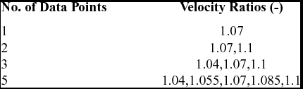
The MCMC will search the parameter space for values of these two parameters, which best allow the HDHB to replicate the experimental data. The HDHB is computed using one harmonic. The experimental data points are, in fact, LCO amplitudes, which are simulated using our model, but it is assumed that the true parameter values are not known a priori. The different data points are computed using these true values at different velocities yielding different values of amplitude. We assume the values of velocity from which each data point originates are known. The velocities of the data points are listed in Table 1. As the same model is used to create the experimental data and drive the MCMC algorithm, the noise term in the statistical model is neglected. This will allow a clearer interpretation of the errors arising in the parameter estimations due to the use of MCMC. Despite neglecting the noise term, a standard deviation must still be defined in order to provide some control of sample acceptance rates via Equation (3); a non-dimensionalised value of 0.01 is used.
Aerofoil - Velocity ratio data points

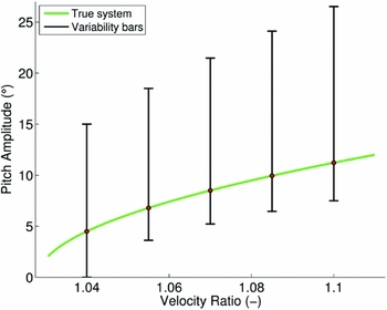
When no experimental data is available, our prior knowledge of the system is the only resource for predicting suitable values for these parameters. Here, the probability of a parameter taking any value within its possible range is assumed to be equal, so uniform distributions are assigned to each variable; hence, the initial distribution encompasses the entire parameter space. This represents an uninformative prior and has no influence on the shape of the posterior distribution. As the true values of the parameters are not known, the parameter space covers a wide range to ensure that it contains the true values. The space ranges from 1 to 7 for cubic stiffness and 0 to 0.5 for damping ratio. The variability of LCO amplitude contained within the parameter space is shown in Fig. 1 and, as expected, a significant amount of variability is present.
Aerofoil - Uncertainty bars for amplitude variability under prior on βα, ζα.

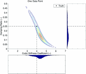
Figure 2 shows the posterior parameter distributions computed by Bayesian inference when one experimental data point is considered, i.e. at a velocity ratio of 1.07. The colouring of the posterior in Fig. 2 uses red to represent high probability and blue to represent low probability. The white regions outside of the contours indicate a close to zero probability that the model can replicate the experimental data based on the observations. The histograms in Fig. 2 show the marginal posterior on each parameter individually when one data point is considered; a reduction of 35.6% in the range of the cubic stiffness distribution is observed while only a reduction of 3.4% is exhibited for damping ratio. It is important to note that the parameter histograms alone do not illustrate the extent of the reduction in variability because the histograms do not provide any information on the correlation between parameters. Solely from the histograms, it can be inferred that the true value lies within a rectangular region, which is 37.9% smaller than the prior parameter space. Immediately, from examining the contour plot, it is obvious that a much greater reduction has occurred, approximately 94.2%. This is due to the slender profile of the posterior, which is caused by the direct influence of each parameter on LCO amplitude; as one parameter changes, the other must also change to allow the model to perform well.
Aerofoil – Posterior and parameter distributions using data from one velocity.

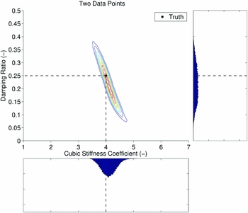
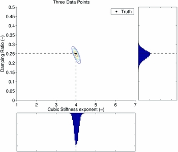
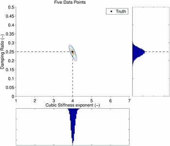
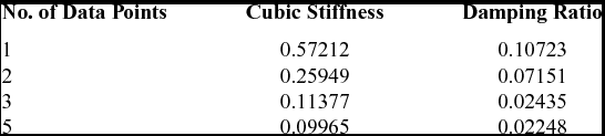
After including two experimental points at the velocities 1.07 and 1.1, a further clear reduction in the spread of the two variables is shown in Fig. 3. The spread of the cubic stiffness coefficient is less than that of the damping ratio, which suggests that the system is more sensitive to the cubic stiffness – see the standard deviations in Table 2. The addition of another point, at a velocity ratio of 1.04, yields another refinement of the posterior distribution as shown in Fig. 4. The posterior and histograms for five data points are shown in Fig. 5. These show probability distributions which are approximately Gaussian and converge towards the true parameter values. The reduction in parameter range with an increasing number of data points is also evidenced by the standard deviations of the posterior distributions as shown in Table 2.
Aerofoil – Posterior and parameter distributions using data from two velocities.

Aerofoil – Posterior and parameter distributions using data from three velocities.

Aerofoil – Posterior and parameter distributions using data from five velocities.

Aerofoil – Standard deviation of input parameters

The selection of a single best parameter value is open to debate; numerous approaches can all be justified(Reference Bol’shev27). However, the true values can be said to be contained within the posterior distribution with high probability, providing the observations are accurate. Thus, if the model performs well for all parameter values within the posterior region, the Bayesian inference has been a success. In this work, two methods for extracting the deterministic values from the result will be investigated: the means of the marginal parameter distributions and the values that yield the maximum posterior, known as the Maximum A-Posteriori (MAP) estimate.
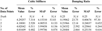
Table 3 shows the extracted parameter values using these two selection criteria. It is clear that the introduction of new experimental evidence enables the posterior distributions to converge to the true values using both techniques, providing the evidence is not contradictory. Closer inspection of Table 3 shows a gradual convergence of the mean parameter values to the true value as expected. Conversely, the MAP estimate provides an inaccurate prediction for one data point but very accurate predictions when two or more data points are considered. This illustrates how effective MAP estimates can be when the posterior is well-identified. When only one data point is considered, MAP performs poorly because the locus of parameter combinations that allow the model to perform perfectly is not a single discrete point. For two random parameters, optimal combinations lie along a line that is contained within the red region of the contour plot in Fig. 2. As the MAP will return the sample that performed best, it will be located near this optimal line but not necessarily near the true values. When enough data points are considered to reduce the locus of optimal parameters to a single discrete point (two points for a two-dimensional problem), MAP will produce an accurate prediction of true values.
Aerofoil – convergence of input parameters

For MAP, the predictions may not necessarily improve by including more data points. This unexpected behaviour can be caused by employing a finite number of MCMC samples. Often, the exact true parameter values are not sampled as a result–only samples located close to the true values. This is the reason why extracting the MAP from a posterior generated in this way is an approximation. Nevertheless, this error is very small and reduces probabilistically with both an increasing number of data points and an increasing number of MCMC samples. From these results, it is suggested that MAP is used when more than one data point is considered. A MAP estimate can also be computed more efficiently by solving an optimisation problem where the maximum value of the posterior is found. However, this approach will not uncover the posterior distribution. A comparison of both estimation methods is recommended to allow the practitioner to gauge how much error could be present in the results.
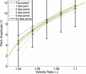
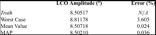
Figure 6 shows the variability in LCO amplitude based on all combinations of parameter values within each posterior distribution. The error bars shown represent the variability from a 98% confidence interval of the posterior. The baseline case (no data points) is the variability from the entire parameter space as shown in Fig. 1. As expected, the performance of the model improves with an increasing number of observations. The model performance improvement is greatest close to the velocities that are considered in the MCMC. Therefore, to ensure the best global model performance, it is important that the experimental data covers a wide range of velocities. Looking at the potential error in the model when only one experimental point is considered, it is clear that the error is smaller at the velocity that corresponds to the data. Likewise, for two experimental data points, the model performance is much better at higher velocities where the calibration takes place. Using three data points gives, globally, a small error as the velocities that were considered span the entire range of the velocities of interest. The performance of the MCMC using five data points gives a worst-case variability of 7.3%. Note that all of the standard selection criteria mentioned above would produce a model that has significantly less error than the worst case. This is illustrated in Table 4 where the corresponding errors for the MAP and mean value criteria are displayed.
Aerofoil - Uncertainty bars for variability across posterior distributions.

Aerofoil – LCO prediction error using five data points at
 ${\bm V=1.07}$

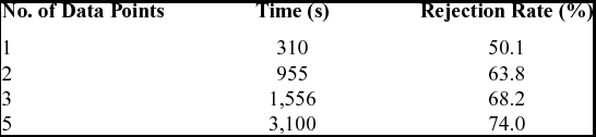
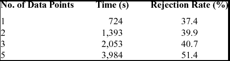
Table 5 shows the time taken and the rejection rate of the MCMC for a varying number of experimental data points. When additional observations are considered, more model evaluations are required. In this case, the cost of the analysis is tractable and could be extended to include more data points or MCMC samples easily.
Aerofoil – Wall clock cost of MCMC, 20,000 samples

5.0 GOLAND WING
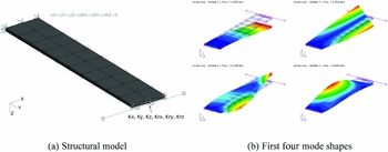
The Goland wing provides a relatively simple 3D model exhibiting several complex aeroelastic phenomenon that are challenging to engineering prediction methods. The wing has a rectangular plan-form with a span of 20 ft and a 6 ft chord. The finite element model of the heavy version of the Goland wing is described in the work of Beran et al(Reference Beran, Knot, Eastep, Synder and Zweber28) and is shown in Fig. 7(a). The structural model used in this work includes localised non-linearities between the tip store attachment stiffness and the wing. The non-linearities are in the form of polynomial laws for spring elements in the translational z-direction (Kz), and the rotational y-direction (Kry) DoF, which were shown to be the most sensitive by Badcock et al(Reference Badcock, Khodaparast, Timme and Mottershead29).
Goland wing.

The equations of motion for the Goland wing take the same form as Equation (5). The external forces,
 $\bf F$
, that act on the wing are aerodynamic in nature. NASTRAN computes these forces in the modal domain using the Doublet-Lattice method. Thus, the wing is analysed in the modal domain; this also significantly reduces the complexity of the problem(Reference Platten, Wright, Worden, Dimitriadis and Cooper30). The transformation between the physical and modal space(Reference Platten, Wright, Dimitriadis and Cooper31) is given as {x} = [Φ]{q}, where
 $\bf \Phi$
is the truncated matrix of eigenvectors, (nm
modes, extracted from NASTRAN) and
 $\bf q$
is a vector of nm
modal coordinates.
The aerodynamic data is only computed for a range of discrete reduced frequencies, so it is represented as a rational function to maintain validity for all values within this range(Reference Eversman and Tewari32). For this investigation, only four structural modes are considered and are shown in Fig. 7(b). The system in the modal domain with modal coordinates,
 $\bf q$
is given as(Reference Badcock, Khodaparast, Timme and Mottershead29,Reference Dimitriadis, Vio and Cooper33) :
 $$\begin{equation}
{\bf {\tilde{M}}}_{\phi } {{\bf \ddot{q}}} + {\bf {\tilde{C}}}_{\phi } {{\bf \dot{q}}} + {\bf {\tilde{K}}}_{\phi } {\bf q} + {\bf K}_{nl}({\bf {q}}) = {\frac{\rho V^{2}}{2}} \sum _{i=1}^{n_{l}}\left[{\bf A}_{i+2}\right]{\bf {\dot{q}}}_{a_{i}},
\end{equation}$$
where
 ${\bf {\tilde{M}}}_{\phi }$
,
 ${\bf {\tilde{C}}}_{\phi }$
,
 ${\bf {\tilde{K}}}_{\phi }$
and K
nl
(q) are the aeroelastic system mass, damping, linear and non-linear stiffness matrices, respectively(Reference Hayes and Marques9). A
• represents the rationally approximated components of the generalised aerodynamic matrix extracted from NASTRAN.
 $\dot{{\bf q}}_{a_{i}}$
are augmented terms arising from the Laplace domain treatment of the generalised aerodynamic matrix and have the relationship:
 $$\begin{equation}
\ddot{{\bf q}}_{a_{i}}={\dot{\bf q}}-{\frac{V}{b}}\eta _{i}\dot{{\bf q}}_{a_{i}}
\end{equation}$$
Equations (21) and (22) can be combined and displayed in state space format:
 $$\begin{equation}
\dot{{\bf w}} + {\bf A}_{\bf s} {\bf w} + {\bf u} = 0 = {\bf R},
\end{equation}$$
where
 $$\begin{equation*}
{\bf w} = \left\lbrace \begin{array}{c}\bf q\\
{\dot{\bf q}}\\
-{\bf A}_{3}\dot{{\bf q}}_{a_{1}}\\
-{\bf A}_{4}\dot{{\bf q}}_{a_{2}}\\
\vdots \\
-{\bf A}_{n_{l}+2}\dot{{\bf q}}_{a_{n_{l}}} \end{array}\right\rbrace ,\ \ {\bf u} = \left\lbrace \begin{array}{c}\bf 0 \\
{{\bf {\tilde{M}}}_{\phi }}^{-1} {{\bf \Phi }}^{\mathrm{T}} {\bf K}_{nl}({\bf q}) \\
{\bf 0} \\
{\bf 0} \\
\vdots \\
{\bf 0} \end{array} \right\rbrace
\end{equation*}$$
and
 $$\begin{equation*}
{\bf A}_{s} = \left[ \begin{array}{c@{\quad}c@{\quad}c@{\quad}c@{\quad}c@{\quad}c}\bf 0&-{\bf I}&{\bf 0}&\dots &\dots &{\bf 0}\\
[0.2em]{{\bf {\tilde{M}}}_{\phi }}^{-1}{\bf {\tilde{K}}}_{\phi }&{{\bf {\tilde{M}}}_{\phi }}^{-1}{\bf {\tilde{C}}}_{\phi }& {{\bf {\tilde{M}}}_{\phi }}^{-1}{\frac{\rho V^{2}}{2}}{\bf I} & \dots & \dots & {{\bf {\tilde{M}}}_{\phi }}^{-1}{\frac{\rho V^{2}}{2}}{\bf I}\\
[0.3em]{\bf 0}&{\bf A}_{3}&{\frac{V}{b}}\eta _{1}{\bf I}& {\bf 0}&\dots &{\bf 0}\\
{\bf 0}&{\bf A}_{4}&{\bf 0}&{\frac{V}{b}}\eta _{2}{\bf I}& \ddots &\vdots \\
\vdots &\vdots &\vdots &\ddots &\ddots & {\bf 0}\\
{\bf 0}&{\bf A}_{n_{l}+2}&{\bf 0}&\dots &{\bf 0}&{\frac{V}{b}}\eta _{n_{l}}{\bf I} \end{array} \right]
\end{equation*}$$
Applying the HDHB method to Equation (21) yields the system:
 $$\begin{equation}
[{\bf {\tilde{M}}}_{\phi } {\bf E}_{acc}^{-1} + {\bf {\tilde{C}}}_{\phi } {\bf E}_{vel}^{-1} + {\bf {\tilde{K}}}_{\phi }{\bf E}_{def}^{-1}]{\hat{\bf Q}_{\phi }} + {\bf E}_{def}^{-1} {\hat{\bf K}}_{nl} - {\frac{\rho V^{2}}{2}} \sum _{i=1}^{n_{l}}\left[{\bf A}_{i+2}\right]{\bf E}_{def}^{-1} {\hat{\bf Q}}_{a_{i}}=0
\end{equation}$$
E
−1
acc
, E
−1
vel
and E
−1
def
are transformation matrices shown in(Reference Hayes and Marques9). The complexity of both the non-linear stiffness force,
 $\lbrace {\hat{\bf K}}_{nl}\rbrace$
, and the decomposed generalised aerodynamic vectors,
 $\lbrace {\hat{\bf Q}}_{a_{i}}\rbrace$
, prevent the straightforward representation of these terms in the frequency domain. Subsequently, Equation (24) is a time domain representation of the problem, where the non-linear terms are represented as reconstructed Fourier series. The Fourier coefficients are formed using DFT and are computed numerically as described in the work of Hayes et al(Reference Hayes and Marques9). Equation (24) is solved simultaneously for 2NH
+ 1 equally spaced time steps across one period with
 $t_{i}={\frac{i2\pi }{2n_{H}+1}},\ (i=0,1,\ldots ,2N_{H})$
to maintain temporal accuracy. A Newton-Raphson scheme is employed as per the previous case; the response frequency is maintained as a variable by locking the cosine Fourier coefficient of the first harmonic of the first mode to zero.
5.1 Results
As in the aerofoil case, the parameters of interest here are the cubic stiffness and damping coefficient of the wing. More specifically, the exponent of the cubic stiffness in the translational z direction, az
β, and the coefficient of the damping matrix,
 ${\check{\bf C}}_{\phi }$
, given by d are considered. The parameter values for this case are the same as the deterministic case described by the authors in a previous work(Reference Hayes and Marques9). Subsequently, the true value for the cubic stiffness exponent is az
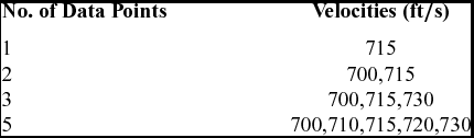
β = 10.954243 and the damping ratio has a true value of d = 0.1. The velocities of interest for this case are shown in Table 6.
Goland wing - Velocity data points

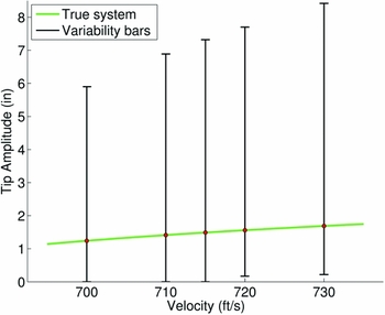
The time domain formulation of the Goland wing described above is used to generate the experimental data and the HDHB formulation is used to drive the MCMC. Again, there is assumed to be no noise associated with the data due to the excellent agreement between the HDHB and time domain models as previously demonstrated by Hayes and Marques(Reference Hayes and Marques9). The parameter space is given to span from values of 9.5 to 12.5 for the cubic stiffness exponent and from 0.05 to 0.95 for the damping coefficient, respectively. The variability in LCO amplitude as a result of the possible range of these parameters at the velocities of interest is shown in Fig. 8. This data is computed using the HDHB method with one harmonic. As in the aerofoil case, the variability is extensive.
Goland wing – Uncertainty bars for variability across entire parameter space.

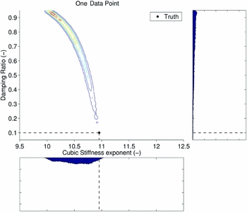
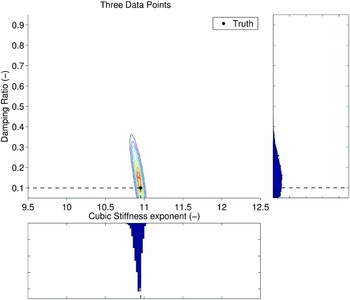
The MCMC parameters are the same as in the aerofoil case with 20,000 MCMC samples being employed with a burn-in of 1,000 samples. Figure 9 shows the posterior contour plot and histograms for the case of one data point at a velocity of 715 ft/s. As in the aerofoil case, it is evident that the posterior has a non-trivial slender profile, which suggests a notable dependence of LCO amplitude on both input parameters. From the histograms in Fig. 9, a reduction of 63.5% in the size of parameter space is exhibited while the contour plot shows a reduction of 92.7% reiterating the importance of observing the shape of the posterior. The cubic stiffness histogram resembles a Gaussian distribution while the damping ratio distribution is heavily skewed with a small percentage of samples located near the true value. As the time domain agrees well with the HDHB results, this result is known to be caused by the employment of an insufficient number of MCMC samples. Using a larger number of MCMC would ensure that the entire posterior would be sampled by the MCMC.
Goland wing – posterior and parameter distributions using data from one velocity.

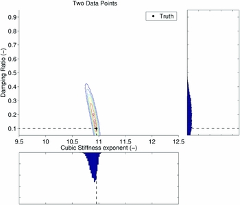
Including another data point at a velocity of 700 ft/s shows another significant reduction in the size of the posterior distribution, as illustrated in Fig. 10. The histograms exhibit Gaussian behaviour for both parameters in contrast to Fig. 9. The cubic stiffness exponent histogram peaks in the vicinity of the true value of 10.954243 while the damping ratio histogram peak is located above the true value of 0.1.
Goland wing – Posterior and parameter distributions using data from two velocities.

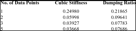
Including more velocity data points further refines the posterior distribution as shown by the standard deviations in Table 7 and the contour plots and histograms in Figs 11 and 12. Notably, the damping histogram peaks still contain significant discrepancies from the true damping value. This is a result of this implementation of the MCMC algorithm, which enforces parameter space boundaries. When the current sample is close to the boundary, the next sample may be chosen to be placed outside of the parameter space. If this occurs, the algorithm will place the sample on the boundary. Therefore, all the samples that should be outside of the parameter space will be generating the next sample from the boundary and this shifts a portion of the samples farther from the boundary than they would be otherwise. Hence, the distribution can be shifted and subsequently an error is introduced into the prediction of true values using a mean or modal selection criteria. This emphasises the importance of ensuring that the chosen parameter space contains the entire range of possible values within it. If the posterior interferes with the chosen parameter space, it is essential that the practitioner is aware to correctly interpret the results or adjust the boundary constraints.
Goland wing – Posterior and parameter distributions using data from three velocities.

Goland wing – Posterior and parameter distributions using data from five velocities.

Goland wing – Standard deviation of input parameters

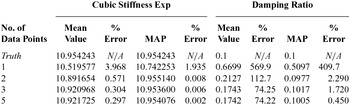
Comparing the selection criteria in Table 8 also illustrates that truncation of the distribution at the parameter space boundary shifts the mean. The mean values for damping ratio do converge toward the true value but remain an inaccurate estimate after five data points with an error of 74.22%. Note, the MAP is unaffected by this shifting and still performs very well when two or more data points are considered. The cubic stiffness exponent, not interfering with its corresponding boundary, is unaffected by the shifting of samples as evidenced by the convergence of the mean value to a high level of accuracy with an increasing number of data points. Note, the MAP performs better than the mean value prediction method as in the aerofoil case when more than one data point is considered and in this case, it is two orders of magnitude more accurate.
Goland wing – Convergence of input parameters

The variability in LCO amplitude as a result of propagating the posterior distributions through the HDHB model is shown in Fig. 13. Two similarities with the aerofoil case are apparent, see Fig. 6. Firstly, each additional data point introduces a reduction in LCO amplitude variability across all velocities, which is synonymous with the posterior decreasing in size. Secondly, the greatest reduction in variability occurs within the velocities spanned by the data points as illustrated by the line for two data points; variability is larger at 730 ft/s because the inference only considered velocities up to 715 ft/s. However, there is an additional characteristic to the behaviour occurring in Fig. 13, which is not apparent in the aerofoil case. The upper variability bars are closer to the true system at lower velocities and the lower variability bars are closer at higher velocities. This type of behaviour must be caused by the interaction of the input parameters on the LCO amplitude and the shape of the posterior.
Goland wing – Uncertainty bars for variability across posterior distributions.

Figure 14 shows the LCO behaviour of the Goland when each input parameter is perturbed individually from the true system. The damping ratio is perturbed by twice as much as the cubic stiffness exponent to account for the difference in parameter sensitivity. From inspection of Fig. 14, it is evident that LCO behaviour becomes more sensitive to cubic stiffness at higher velocities due to the higher LCO amplitude and damping ratio becomes less influential as velocity increases; this contributes to the skewed behaviour. To understand how, consider the shape of the posterior in Fig. 9. It has two extreme conditions that are responsible for the range of observed variability: high cubic stiffness with low damping and low cubic stiffness with high damping. At 715 ft/s, these extreme parameter combinations cancel each other out to allow the model to perform. As the posterior extends much farther from the true values in the direction of high damping and low cubic stiffness, this extreme condition is much more susceptible to changes in the influence of each parameter at different velocities. Consider this condition when the posterior distribution is propagated through the model at 730 ft/s. The large increase in damping ratio that occurs will have less of a suppressing effect on the LCO amplitude due to the behaviour in Fig. 14. Additionally, the amplifying effect due to the large decrease in cubic stiffness will be exacerbated by the growing influence of cubic stiffness at high velocities. The resulting LCO amplitude is much higher than what is expected if only information from 715 ft/s is considered. At 700 ft/s, the suppression due to high damping is amplified and the destabilisation due to lower stiffness is reduced. As the other extreme point on the posterior distribution is so close to the true values, this suppression and amplification behaviour is not prevalent.
Goland wing – Velocity sweeps of perturbed cubic stiffness and damping coefficients.

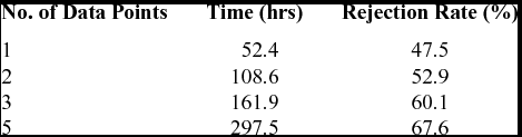
The computational time taken for each analysis for the Goland wing is shown in Table 9. Note, the Goland wing times are much longer than in the aerofoil case with over 12 days needed to run the analysis for five data points. The practicality of the MCMC strategy is directly influenced by the cost of the model evaluations, which must be kept to a minimum. Hence, for models of higher complexity, some type of reduced order model should be used. Note, these computations were performed on a single CPU processor and it is possible to parallelise the simulations for each MCMC sample when multiple data points are considered; this improves with the scalability of the method in terms of the number of data points used. Further inspection of Table 9 shows slightly smaller rejection rates in comparison to the aerofoil case, see Table 5. This is determined by: how closely the proposal distribution matches the shape and size of the posterior, and the experimental noise value used in the calculation of the likelihood in Equation (3).
Goland wing – Wall clock cost of MCMC, 20,000 samples

6.0 GOLAND WING WITH NORMAL MODES VARIABILITY
The final case in this work also considers the Goland wing from the previous section. In the last case, the non-linear stiffness and damping behaviour of the wing were hard-wired in the dynamic model. However, structural variability is now imposed at the FE analysis stage to generate new mode shapes and modal frequencies for the aeroelastic simulations. The cubic stiffness coefficients in the z-axis direction (Kz) and rotation about the y-axis (Kry) were given values of 1010.954243 and 1010, respectively. There is no non-linear component of damping in this work, but the linear damping matrix,
 $ {\bf {\tilde{C}}}_{\phi }$
is given a damping coefficient of 0.1. Previous work investigated eight structural parameters and identified the two most sensitive parameters with respect to the onset of flutter to be the trailing-edge spar thickness and the store CG chord-wise location(Reference Hayes and Marques9); these were retained in this work and were given the true values of 0.0006 ft and 0 ft, respectively. The parameter space was given bounds of 0.0004 ft to 0.0008 ft for the trailing-edge spar thickness and − 0.125 ft to 0.125 ft for the store centre of gravity.
Due to the additional computational time needed for the re-evaluation of the mode shapes in NASTRAN, the cost of running the MCMC using the HDHB would be excessive. To mitigate this, an Artificial Neural Network (ANN)(Reference Segaran34) was trained using 5,000 LHS from the selected parameter space, which took 23.6 hours to generate on a single processor. The generation of the training samples can be heavily parallelised thus vastly reducing the computational time. The training of the ANN took 7.7 hours and analysis showed a mean error of 0.02% with a standard deviation of 1.1%, which was deemed acceptable. In contrast to the previous cases, the discrepancy between the ROM predictions at the true values and the experimental data is not negligible, hence the error term from Equation (3) is included. The error term is defined as a Gaussian with mean 0 and a normalised standard deviation of 0.02 to produce high sample acceptance rates. This will allow the model to make better predictions when there is a discrepancy between the model and data. However, this can incur a penalty in MCMC convergence.
In this case, the sensitivity of LCO amplitude differs significantly with respect to each parameter. This suggests that the MCMC will require more samples to reach statistical convergence. As an evaluation of the ANN for a given set of inputs is very cheap in comparison to the HDHB simulations, this case employs 40,000 MCMC samples with a burn-in phase of 5,000 samples. The experimental data in this case is a series of simulations performed at different velocities using the time-domain solver employed in a previous publication(Reference Hayes and Marques9). The time domain simulations took approximately 160 s each whereas the HDHB took 17 s per sample, hence the HDHB is much more suitable for training the ANN. The HDHB samples were computed using one harmonic and the majority of the time taken for a sample is spent on the FE analysis to create the new mode shapes and frequencies as only the LCO prediction phase of each sample is sped up. The velocities of interest remain the same as in the previous case and are displayed in Table 6.
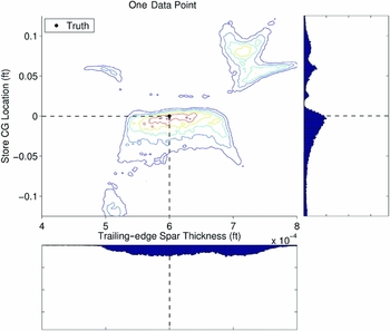
The posterior distribution and histograms for one data point at 715 ft/s are shown in Fig. 15 where the store CG location represents a translation in the chord-wise direction from the nominal position of 0.25 ft downstream of the leading edge. Positive translation denotes movement towards the trailing edge. Immediately, it is evident that the posterior takes a radical form, much more complex than in the previous cases. This is caused by the indirect interaction between fundamental structural parameters and the LCO prediction. The store CG location in particular has a highly non-linear relationship with stability due to a significant change in the mode shapes of the structure; changing the mode shapes alters the way the structure interacts with the flow and this is the source of the peculiar posterior shape. Evidence of the mode shape variability induced by changes in these structural parameters has been shown by previous work of Hayes et al.(Reference Hayes, Marques and Yao35). It is possible to see an underlying trend amongst the distinctive shape of the posterior; most of the regions of medium to high probability show a positive correlation between the two parameters. As the store CG location moves towards the trailing edge, stability will decrease, thus spar thickness also needs to increase to compensate for the change in stability.
Goland wing with changing mode shapes – Posterior and parameter distributions using data from one velocity.

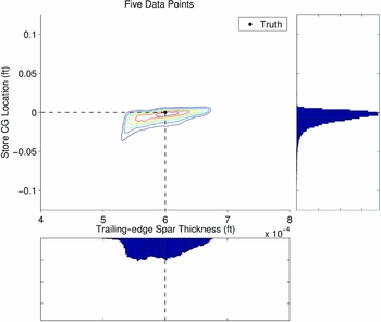
The distributions and histograms for two, three and five points are shown in Figs 16–18, respectively. It is evident from the posterior plots that the distribution is reduced in size when more points are considered, as in the previous cases. When the low velocity of 700 ft/s is introduced, the regions of high store CG location are removed as the model fails to coincide with the time domain solution at this velocity. Further refinement from adding more velocities restricts the posterior to a narrow range of store location and quite a wide range of spar thickness. As a result, it is concluded that the store location is the more important factor for model performance and this is concurrent with results shown previously by the authors in Hayes et al(Reference Hayes, Marques and Yao35).
Goland wing with changing mode shapes – Posterior and parameter distributions using data from two velocities.

Goland wing with changing mode shapes – Posterior and parameter distributions using data from three velocities.

Goland wing with changing mode shapes – Posterior and parameter distributions using data from five velocities.

Inspection of the histograms in Figs 16–18 illustrate the reduction of the store CG location variability with increased data points. The corresponding distributions develop into well-formed skewed Gaussian distributions with the modal values in the vicinity of the true value and minimal samples above the true value. This is due to the decrease in stability that occurs when the store location is moved towards the trailing edge. As stability decreases, the LCO amplitude becomes more sensitive to variability thus the model’s predictions will degrade quicker than when the store is moving towards the leading edge. There is only a small refinement of the trailing-edge spar thickness distribution when the number of data points is increased as it is the less influential parameter. There is a dip observed in the spar thickness distribution shape when five velocities are considered near the true value. This is believed to be caused by the low impact this parameter has on the acceptance of a sample at these conditions. As a result, more MCMC samples are required to accurately model the posterior distribution for this parameter. The addition of further samples should eradicate this dip.
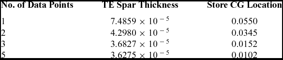
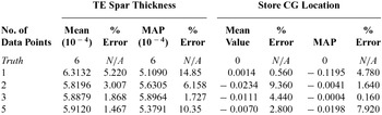
Although the analysis would benefit from more MCMC samples, the ability to estimate the true parameter value has not been compromised significantly as shown in Tables 10 and 11 where the mean values of the distributions move closer towards the true values and standard deviation decreases. The mean value for store CG location for one data point is in fact the closest to the true value of 0 ft, but this is not considered to be meaningful because of the radical shape of the distribution. It is worth mentioning that the percentage error for the store CG location is normalised using the width of its prior, i.e. 0.25 ft.
Goland wing with changing mode shapes – Standard deviation of input parameters

Goland wing with changing mode shapes – Convergence of input parameters

The MAP predictions show different behaviour than previously observed where the method does not achieve the same levels of accuracy as shown in the other cases. This is attributed to the presence of the experimental noise term in this case; it will shift the output of the model, hence, the best sample will not be at the true values. From inspection of the mean value result, the error shown in the case of MAP with five data points is too large to be caused by the experimental noise for both TE spar thickness and store location. This shows that although the ANN is relatively accurate across the parameter space as a whole, it contains local inaccuracies at velocities previously not considered. The posterior value in this region will be reduced allowing the MAP to choose a sample with mediocre performance in every velocity. Nevertheless, it has effectively located the vicinity of the true values. If warranted, another MCMC could be carried out with full order simulations and a refined parameter space.
The computational times for each case are shown in Table 12. The times are comparable with that of the aerofoil case even though there are almost twice as many samples in the Goland wing highlighting the benefit of the ANN. The rejection rates are lower than that of the aerofoil case that performed very well; this is due to the size of the proposal distribution. Here, the proposal distribution is smaller than the posterior, which leads to an increased acceptance rate allowing the required amount of MCMC samples to be reached sooner. However, this has the disadvantage of increasing the dependence between consecutive samples, requiring more thinning of the chain.
Goland wing with changing mode shapes – Wall clock cost of MCMC, 40,000 samples with ANN

7.0 CONCLUSIONS
Estimations of various structural linear and non-linear parameters were conducted for a pitch/plunge aerofoil (one case) and Goland wing configuration (two cases) based on LCO behaviour. A Bayesian inference methodology with MCMC was employed that utilised experimental data to reduce the parameter distributions. The experimental data was simulated using the model for the aerofoil case and a time marching code for the Goland wing. The efficiency of the HDHB method was exploited to cheaply drive the MCMC in the aerofoil and first Goland wing cases. For the second Goland wing case, HDHB was used to train an ANN that was used for the MCMC. In all cases, it was evident that the addition of more experimental data refined the posterior distribution allowing variability in the LCO amplitude to be significantly reduced. More observations also improved the estimation of the true parameter values using a mean value criterion. However, this criterion is susceptible to errors arising if the posterior distribution interferes with the parameter boundary.
Parameter estimation using MAP is more accurate than mean value selection, provided enough data points are considered and the experimental noise is sufficiently small. Furthermore, MAP is unaffected by any parameter boundary interaction with the posterior, but it is more likely to change when the experimental noise term is larger as the comparison between predictions and observations is affected. Additionally, it is more sensitive to localised model inaccuracies with respect to a single data point. It is recommended that the practitioner employs both methods or validates against the posterior plot to gauge the level confidence in the estimation.
When quantifying the reduction in variability of the input parameters (especially stochastic parameters), 1D histograms alone cannot convey the true reduction when data points are added nor do they effectively uncover interdependencies between the parameters of interest. Hence, examination of the shape of the posterior is necessary to correctly quantify the reduction in variability that has been achieved. The standard deviations of the parameter distributions give an indication of the sensitivity of LCO amplitude with respect to each parameter. The importance of the proposal distribution size and shape with respect to the MCMC convergence rate and statistical validity was highlighted. The Bayesian inference performed well and was shown to be a feasible approach to reduce the uncertainty associated with structural parameters for this kind of dynamic problems.
ACKNOWLEDGEMENTS
The first author would like to thank the Department for Employment and Learning for Northern Ireland for funding his research.