Nomenclature
- b
wing span (m)
-
 $L$
,
$N$
-
moments around
$x$
,
$z$
body axis (N
$\cdot$
m) - p, r
angular rates (rad/s)
-
$\bar {q}$
-
dynamic pressure (N/m
$^2$
) -
$F_T$
-
electric propulsor thrust (N)
-
$M_p$
-
maximum overshoot (
$\%$
) - S
-
reference wing area (m
$^2$
) -
$T_s$
-
settling time (s)
-
$\mathbf{u}$
-
control vector
-
$\mathbf{x}$
-
state vector
-
$\mathbf{z}$
-
augmented state vector for RS-LQR


Greek symbol
-
$\alpha ^*$
-
robustness measure
-
$\beta$
-
sideslip angle (rad)
-
$\gamma$
-
yawing-moment equalisation factor
-
$\delta _a$
-
aileron deflection (rad)
-
$\delta _r$
-
rudder deflection (rad)
-
$\zeta$
-
damping ratio
-
$\eta$
-
weight parameter
-
$\phi$
,
$\psi$
-
Euler angles (rad)
-
$\sigma$
-
singular value
-
$\omega$
-
bandwidth or natural frequency (rad/s)


1.0 Introduction
The aviation industry currently contributes approximately 3% of global carbon emissions, and this figure is projected to triple by 2050 in the absence of effective countermeasures [Reference Huang, Zhang, Wang and Zhou1, Reference de Heer, de Visser, Hoogendoorn and Jentink2]. In response, the development of environmentally sustainable aircraft, such as hydrogen-fueled and electric aircraft, has become increasingly important. Among these, distributed electric propulsion (DEP) aircraft have emerged as a promising solution due to their ability to utilise electric power and improve redundancy through multiple propulsors [Reference Kim, Lee and Park3].
DEP configurations can be classified into four categories based on the placement and usage of the propulsion system: multi-rotor, tilt-lift, stopped-rotor and fixed-wing [Reference Shadbolt4]. Examples include the Volocity [5], VX4 [6], Cora [7] and ES-19 [8], each of which uses distributed thrust differently to achieve vertical takeoff and landing (VTOL), transition or cruise flight (see Figure 1). One of the most distinctive control strategies enabled by DEP is powered yaw control, where differential thrust among electric propulsors is used to generate the desired yawing moment. This approach exploits the fast torque response of electric motors to achieve rapid and precise yaw control [Reference Kou, Wang and Liang9, Reference Vechtel and Buch10]. In addition, it enhances fault tolerance by enabling continued yaw authority even under partial propulsion failure. However, the use of distributed thrust introduces dynamic coupling, actuator redundancy and nonlinear interactions, which increase the complexity of control design and may reduce system robustness.
Several studies have addressed powered yaw control strategies tailored to DEP systems. Cong Yuan et al. [Reference Yuan, Du, Huangfu, Gong, Gao and Li11] proposed a distributed consensus-based method for cooperative thrust regulation, achieving effective yaw and cruise control. Zhang et al. [Reference Zhang, Qu, Du, Fan, Li and Huangfu12] applied pinning-based consensus with prescribed performance control (PPC), demonstrating robustness against external disturbances. Kou et al. [Reference Kou, Wang and Liang9] developed a hierarchical model predictive control (MPC) approach for powered yaw control, while Loder et al. investigated asymmetric thrust control within turbo-electric DEP microgrids to enhance yaw flexibility [Reference Loder, Bollman and Armstrong13].
In parallel, robust control strategies have become increasingly important for DEP aircraft, as these systems are subject to nonlinearities, uncertainties and actuator faults. Liu et al. [Reference Liu, Wang, Zhang and Yin14] proposed a constraint-based adaptive robust prescribed performance control (CARPPC) method for tilt-rotor aircraft during transition, while Sun et al. [Reference Sun, Gui, Lu and Chen15] introduced a fault-tolerant control scheme that addresses uncertainties in electric actuation systems using nonlinear robust design. Tran et al. [Reference Tran, Sakamoto, Sato and Muraoka16] developed a robust output regulation-based augmentation system for a quad-tilt-wing unmanned aerial vehicle (UAV), and Chen et al. [Reference Chen and Jia17] combined Robust Servo LQR (RS-LQR) and Extended State Observer (ESO) for robust tilt-rotor control under actuator saturation and disturbances. Additional contributions include robust transition control for tail-sitter UAVs [Reference Yang, Zhu, Yuan, Wang, Kuang and Shi18], incremental nonlinear control allocation (INCA) for DEP aircraft [Reference de Heer, de Visser, Hoogendoorn and Jentink2] and a gain-scheduled RS-LQR framework for VTOLs [Reference Cook and Gregory19].
However, as mentioned earlier, powered yaw control based only on distributed thrust may be less robust against uncertainties and structural failures than classical flight control approaches using aerodynamic surfaces. This issue is revisited in Section 3. Therefore, unlike the existing works, this study proposes a hybrid-powered yaw control method that combines aerodynamic and electric control actions to improve both robustness and performance. To the best of the authors’ knowledge, no previous powered yaw control method has partially used aerodynamic forces to explicitly improve a robustness measure. Note that many DEP aircraft, as seen in Figure 1, have aerodynamic surfaces that could be used to assist the powered yaw control. Furthermore, this study proposes a fault-tolerant control (FTC) framework that reduces the effect of one or more electric propulsor failures by equalising the yawing moments generated by individual propulsors. Such yawing-moment equalisation for FTC of DEP aircraft has not been reported in the literature.
Examples of distributed electric propulsion (DEP) aircraft: (a) Volocity; (b) VX4; (c) Cora; (d) ES-19.

As a result, the present work has the following clear contributions:
-
(1) Robustness quantification using the minimum singular value of the return difference matrix, which serves as a multiple-input multiple-output (MIMO) robustness metric related to gain and phase margins;
-
(2) A hybrid-powered yaw control method that combines aerodynamic and electric control actions through input-weighting design;
-
(3) A real-time fault detection and controller reconfiguration algorithm based on yawing-moment deviations;
-
(4) A yawing-moment equalisation algorithm that reduces the impact of propulsor failures by distributing yaw contributions more uniformly;
-
(5) Validation of the proposed controller through MATLAB–FlightGear co-simulation and hardware-in-the-loop-simulation (HILS), including system identification of the H4 Hercules flight model.
The proposed methods improve the robustness and fault tolerance of yaw control in DEP aircraft. The structure of this paper is as follows. Section 2 introduces the dynamic equations of the NASA X-57 Maxwell, a representative DEP aircraft. Section 3 presents the proposed hybrid yaw control method based on robustness metrics and response performance. Section 4 presents an FTC method for powered yawing scenarios, which incorporates both fault detection and controller reconfiguration strategies. Finally, Section 5 validates the proposed controller through software-in-the-loop simulation (SILS) using MATLAB integrated with FlightGear and HILS using Raspberry Pi.
Trim conditions of X-57 Maxwell

Table 1. Long description
A table listing trim conditions for the X-57 Maxwell aircraft. The table has 12 rows and 5 columns. The columns are labeled Notation, Definition, Value, and Unit. The rows list various trim conditions with their corresponding values and units. Row 1: V 0, Trim velocity, 77.11, m/s. Row 2: theta 0, Trim pitch angle, 0.29, deg. Row 3: alpha 0, Trim angle of attack, 0.29, deg. Row 4: delta e 0, Elevator trim deflection, 3.46, deg. Row 5: F T x 0, Cruise propulsor thrust (per motor), 511.55, N. Row 6: F T h 0, High-lift propulsor thrust (per motor), 221.08, N. Row 7: beta 0, Trim sideslip angle, 0, deg. Row 8: p 0, Trim roll rate, 0, deg/s. Row 9: r 0, Trim yaw rate, 0, deg/s. Row 10: phi 0, Trim roll angle, 0, deg. Row 11: psi 0, Trim yaw angle, 0, deg. Row 12: h 0, Trim altitude, 2438.4, m.
NASA X-57 Maxwell.

2.0 Lateral equations of motion for distributed electric propulsion aircraft
In this study, the NASA X-57 Maxwell aircraft (Figure 2), which is equipped with 14 electric propulsors and aerodynamic control surfaces (aileron and rudder), is initially used to effectively demonstrate the design of the proposed DEP control methods because it has a large number of propulsors.
The motion of a fixed-wing aircraft is described by the nonlinear six-degree-of-freedom (6-DOF) equations derived from Newton’s laws in a body-fixed coordinate system. These equations are well established in classical flight dynamics literature [Reference Etkin20]. For control design, the nonlinear system is linearised about a steady-state trim condition under the small-disturbance assumption. Let the nonlinear dynamics be expressed as
 \begin{equation} \dot {\mathbf{x}} = \mathbf{f}(\mathbf{x},\mathbf{u}), \end{equation}
and let
 $(\mathbf{x}_{eq}, \mathbf{u}_{eq})$
denote the trim state and input, as listed in Table 1. By defining perturbation variables
 $\Delta \mathbf{x} = \mathbf{x} - \mathbf{x}_{eq}$
and
 $\Delta \mathbf{u} = \mathbf{u} - \mathbf{u}_{eq}$
, and applying a first-order Taylor series expansion, the linearised system is obtained as
 \begin{equation} \Delta \dot {\mathbf{x}} = \mathbf{A}\Delta \mathbf{x} + \mathbf{B} \Delta \mathbf{u}. \end{equation}
In this study, the Jacobian matrices
 $\mathbf{A}$
and
 $\mathbf{B}$
are evaluated numerically following the procedure described in [Reference Nguyen Van, Alazard, Döll and Pastor21, Reference Nguyen Van, Alazard, Döll and Pastor22]. Moreover, the reference emphasises the small-angle perturbation assumption as a necessary condition for preserving linearity when linearising the nonlinear model. Accordingly, this study rigorously incorporates this assumption to ensure that the small-angle perturbation condition is satisfied under all operating conditions (e.g.
 $\psi _{ref} = 10^\circ$
). For the specific case of the NASA X-57 Maxwell aircraft, the trim condition and aerodynamic stability and control derivatives are obtained from [Reference Kou, Wang and Liang9]. Based on these parameters, the linearised state-space model is constructed for subsequent control design. For notational brevity, the perturbation variables
 $\Delta \mathbf{x}$
and
 $\Delta \mathbf{u}$
are hereafter denoted simply by
 $\mathbf{x}$
and
 $\mathbf{u}$
, respectively.
2.1 Fixed-wing mode dynamics
The fixed-wing mode dynamic equations of the NASA X-57 Maxwell can be expressed in the state-space equation form as shown in Equation (3):
 \begin{equation} \underbrace {\begin{bmatrix} \dot {\beta }\\ \dot {p}\\ \dot {r}\\ \dot {\phi }\\ \dot {\psi } \end{bmatrix}}_{\dot {\mathbf{x}}_{F}} = \underbrace {\begin{bmatrix} \dfrac {Y_{\beta }}{V_0}\;\;\;\;\; & \dfrac {Y_{p}}{V_0}\;\;\;\;\; & -1 + \dfrac {Y_{r}}{V_0}\;\;\;\;\; & \dfrac {g\cos \theta _0}{V_0}\;\;\;\;\; & 0\\[7pt] L_{\beta }\;\;\;\;\; & L_{p}\;\;\;\;\; & L_{r}\;\;\;\;\; & 0\;\;\;\;\; & 0\\ N_{\beta }\;\;\;\;\; & N_{p}\;\;\;\;\; & N_{r}\;\;\;\;\; & 0\;\;\;\;\; & 0\\ 0\;\;\;\;\; & 0\;\;\;\;\; & 0\;\;\;\;\; & 0\;\;\;\;\; & 0\\ 0\;\;\;\;\; & 0\;\;\;\;\; & 0\;\;\;\;\; & 0\;\;\;\;\; & 0 \end{bmatrix}}_{\mathbf{A}_{F}} \underbrace {\begin{bmatrix} \beta \\ p\\ r\\ \phi \\ \psi \end{bmatrix}}_{\mathbf{x}_{F}} + \underbrace {\begin{bmatrix} \frac {Y_{\delta _a}}{V_0}\;\;\;\;\; & \frac {Y_{\delta _r}}{V_0}\\ L_{\delta _a}\;\;\;\;\; & L_{\delta _r}\\ N_{\delta _a}\;\;\;\;\; & N_{\delta _r}\\ 0\;\;\;\;\; & 0\\ 0\;\;\;\;\; & 0 \end{bmatrix}}_{\mathbf{B}_{F}} \underbrace {\begin{bmatrix} \delta _{a}\\ \delta _{r} \end{bmatrix}}_{\mathbf{u}_{F}}. \end{equation}
In the above equation,
 $\mathbf{x}_F$
represents the state variables, including the sideslip angle
 $\beta$
, the roll rate
 $p$
, the yaw rate
 $r$
, the roll angle
 $\phi$
, and the yaw angle
 $\psi$
. The aerodynamic control input
 $\mathbf{u}_{F}$
consists of the aileron and rudder deflections,
 $\delta _a$
and
 $\delta _r$
. Additionally,
 ${V}_0$
,
 $\mathcal{\theta }_0$
, and
 $g$
denote the aircraft’s velocity, pitch angle and gravitational acceleration in the trim condition, respectively. All the other symbols in
 $\mathbf{A}_{F}$
and
 $\mathbf{B}_{F}$
represent aerodynamic constants.
Remark 1. The NASA X-57 Maxwell retains a conventional control architecture, employing a stabilator for pitch and control surfaces for lateral–directional motion, while distributed electric propulsion introduces aero-propulsive coupling through propellers distributed along the wing [Reference Borer24, Reference Frederick, Smith, Yoo, Wallace, Duensing, Housman, Deere and Viken25]. These spanwise propulsion effects modify lift distribution and generate asymmetric thrust, which strongly influence lateral–directional behaviour. In particular, yaw control plays a key role in lateral stabilisation, as roll stabilisation can be achieved through yaw–roll coupling inherent in the aircraft dynamics, as clearly seen in Equation (3). Although distributed propulsion also affects longitudinal aerodynamics, longitudinal control remains mostly governed by conventional aerodynamic mechanisms and is only weakly coupled with lateral–directional dynamics under nominal flight conditions [Reference Stevens, Lewis and Johnson26, Reference Etkin and Reid27]. Therefore, this study focuses on yaw control, which represents the most critical axis influenced by DEP-induced coupling, while pitch stabilisation is not explicitly considered.
2.2 Electric-propulsion mode dynamics
The dynamics of each electric propulsor can be simply represented as a general second-order system [Reference Kou, Wang and Liang9, Reference Freeman and Klunk23], as shown in Equation (4):
 \begin{equation} \ddot {F}_T + 2\zeta _F \,\omega _F\,\dot {F}_T + \omega _F^2\,F_T = \omega _F^2\,F_{T,\mathrm{cmd}}, \\ \begin{bmatrix} \dot {F}_T\\ \ddot {F}_T \end{bmatrix} = \begin{bmatrix} 0\;\;\;\;\; & 1\\ -\omega _F^2\;\;\;\;\; & -2\zeta _F\,\omega _F \end{bmatrix} \begin{bmatrix} F_T\\ \dot {F}_T \end{bmatrix} + \begin{bmatrix} 0\\ \omega _F^2 \end{bmatrix} F_{T,\mathrm{cmd}}. \end{equation}
Here,
 $\zeta _F$
,
 $\omega _F$
and
 $F_{T,cmd}$
represent the damping ratio, the natural frequency and the thrust command of each electric propulsor, respectively. To describe the forces and moments produced by the electric propulsor, the corresponding stability and control derivatives are derived. These stability and control derivatives can be expressed as shown in Equation (5):
 \begin{equation} Y_{T,i} = 0,\quad L_{T,i} = \frac {y_{T,i}\,\sin \theta _{T,i}}{I_{xx}},\quad N_{T,i} = \frac {y_{T,i}\,\cos \theta _{T,i}}{I_{zz}}. \end{equation}
Here,
 $Y_{T,i}$
represents the axial force stability derivative due to the
 $\textit {i}$
-th electric propulsor, while
 $L_{T,i}$
and
 $N_{T,i}$
correspond to the rolling and yawing moment derivatives due to the
 $\textit {i}$
-th electric propulsor, respectively.
 $I_{xx}$
and
 $I_{zz}$
denote the mass moments of inertia about the
 $\textit {x}$
and
 $\textit {z}$
axes, respectively.
 $y_{T,i}$
and
 $\theta _{T,i}$
represent the lateral distance from the aircraft centre of gravity to the
 $\textit {i}$
-th electric propulsion system and its pitch angle, respectively.
Aircraft and propulsor parameters [Reference Kou, Wang and Liang9]

Table 2. Long description
A table listing aircraft and propulsor parameters with their respective values and units. The table has 12 rows and 4 columns. Column headers are Notation, Definition, Value, and Unit. Row 1: Notation, Definition, Value, Unit. Row 2: m_a, Mass of the aircraft, 1360.77, kg. Row 3: S, Reference area, 6.19, m^2. Row 4: b, Reference span, 9.64, m. Row 5: Ixx, Roll moment of inertia, 2215.41, kgm^2. Row 6: Iyy, Pitch moment of inertia, 3874.93, kgm^2. Row 7: Izz, Yaw moment of inertia, 4661.30, kgm^2. Row 8: Ixz, Product of inertia, 0, kgm^2. Row 9: ωcf, Natural frequency (cruise propulsor), 3.73, rad/s. Row 10: ωfh, Natural frequency (high-lift propulsor), 48.12, rad/s. Row 11: ζcf, Damping ratio (cruise propulsor), 0.83, -. Row 12: ζfh, Damping ratio (high-lift propulsor), 0.88, -.
Using these coefficients, the 5-by-28
 $\mathbf{A}_{PF}$
matrix, which describes the variation of 5 state variables in the fixed-wing mode due to the 14 electric propulsors associated with 28 state variables, is expressed in Equation (6). Additionally, the 28-by-28 system matrix
 $\mathbf{A}_{P}$
and the 28-by-14 input matrix
 $\mathbf{B}_{P}$
for the 14 electric propulsors are given in Equation (7). The parameters of the NASA X-57 Maxwell are presented in Table 2.
 \begin{equation} \mathbf{A}_{PF} = \begin{bmatrix} 0\;\;\;\;\; \;\;\;\;\;& 0\;\;\;\;\; & \cdots\;\;\;\;\; & 0\;\;\;\;\; & 0\\ L_{T,1}\;\;\;\;\; & 0\;\;\;\;\; & \cdots\;\;\;\;\; & L_{T,14}\;\;\;\;\; & 0\\ N_{T,1}\;\;\;\;\; & 0\;\;\;\;\; & \cdots\;\;\;\;\; & N_{T,14}\;\;\;\;\; & 0\\ 0\;\;\;\;\; & 0\;\;\;\;\; & \cdots\;\;\;\;\; & 0\;\;\;\;\; & 0\\ 0\;\;\;\;\; & 0\;\;\;\;\; & \cdots\;\;\;\;\; & 0\;\;\;\;\; & 0 \end{bmatrix}\!, \end{equation}
 \begin{equation}\!\!\! \begin{array}{l@{\quad}l} & \mathbf{A}_P = \begin{bmatrix} 0\;\;\;\;\; & 1\;\;\;\;\; & 0\;\;\;\;\; & 0\;\;\;\;\; & \cdots\;\;\;\;\; & 0\;\;\;\;\; & 0\;\;\;\;\; & 0\;\;\;\;\; & 0\\ -\omega _{F,c}^2\;\;\;\;\; & -2\zeta _{F,c}\,\omega _{F,c}\;\;\;\;\; & 0\;\;\;\;\; & 0\;\;\;\;\; & \cdots\;\;\;\;\; & 0\;\;\;\;\; & 0\;\;\;\;\; & 0\;\;\;\;\; & 0\\ 0\;\;\;\;\; & 0\;\;\;\;\; & 0\;\;\;\;\; & 1\;\;\;\;\; & \cdots\;\;\;\;\; & 0\;\;\;\;\; & 0\;\;\;\;\; & 0\;\;\;\;\; & 0\\ 0\;\;\;\;\; & 0\;\;\;\;\; & -\omega _{F,h}^2\;\;\;\;\; & -2\zeta _{F,h}\,\omega _{F,h}\;\;\;\;\; & \cdots\;\;\;\;\; & 0\;\;\;\;\; & 0\;\;\;\;\; & 0\;\;\;\;\; & 0\\ \vdots\;\;\;\;\; & \vdots\;\;\;\;\; & \vdots\;\;\;\;\; & \vdots\;\;\;\;\; & \ddots\;\;\;\;\; & \vdots\;\;\;\;\; & \vdots\;\;\;\;\; & \vdots\;\;\;\;\; & \vdots \\ 0\;\;\;\;\; & 0\;\;\;\;\; & 0\;\;\;\;\; & 0\;\;\;\;\; & \cdots\;\;\;\;\; & 0\;\;\;\;\; & 1\;\;\;\;\; & 0\;\;\;\;\; & 0\\ 0\;\;\;\;\; & 0\;\;\;\;\; & 0\;\;\;\;\; & 0\;\;\;\;\; & \cdots\;\;\;\;\; & -\omega _{F,h}^2\;\;\;\;\; & -2\zeta _{F,h}\,\omega _{F,h}\;\;\;\;\; & 0\;\;\;\;\; & 0\\ 0\;\;\;\;\; & 0\;\;\;\;\; & 0\;\;\;\;\; & 0\;\;\;\;\; & \cdots\;\;\;\;\; & 0\;\;\;\;\; & 0\;\;\;\;\; & 0\;\;\;\;\; & 1\\ 0\;\;\;\;\; & 0\;\;\;\;\; & 0\;\;\;\;\; & 0\;\;\;\;\; & \cdots\;\;\;\;\; & 0\;\;\;\;\; & 0\;\;\;\;\; & -\omega _{F,c}^2\;\;\;\;\; & -2\zeta _{F,c}\,\omega _{F,c} \end{bmatrix}\!, \\ \\ & \mathbf{B}_P = \begin{bmatrix} 0\;\;\;\;\; & 0\;\;\;\;\; & \cdots\;\;\;\;\; & 0\;\;\;\;\; & 0\\ \omega _{F,c}^2\;\;\;\;\; & 0\;\;\;\;\; & \cdots\;\;\;\;\; & 0\;\;\;\;\; & 0\\ 0\;\;\;\;\; & 0\;\;\;\;\; & \cdots\;\;\;\;\; & 0\;\;\;\;\; & 0\\ 0\;\;\;\;\; & \omega _{F,h}^2\;\;\;\;\; & \cdots\;\;\;\;\; & 0\;\;\;\;\; & 0\\ 0\;\;\;\;\; & 0\;\;\;\;\; & \ddots\;\;\;\;\; & 0\;\;\;\;\; & 0\\ \vdots\;\;\;\;\; & \vdots\;\;\;\;\; & \cdots\;\;\;\;\; & \vdots\;\;\;\;\; & \vdots \\ 0\;\;\;\;\; & 0\;\;\;\;\; & \cdots\;\;\;\;\; & \omega _{F,h}^2\;\;\;\;\; & 0\\ 0\;\;\;\;\; & 0\;\;\;\;\; & \cdots\;\;\;\;\; & 0\;\;\;\;\; & 0\\ 0\;\;\;\;\; & 0\;\;\;\;\; & \cdots\;\;\;\;\; & 0\;\;\;\;\; & \omega _{F,c}^2 \end{bmatrix}\!. \end{array} \end{equation}
2.3 Combined dynamics
The complete dynamic equation, combining the fixed-wing and electric-propulsion modes of the NASA X-57 Maxwell, can be expressed in Equation (8):
 \begin{equation} \underbrace {\begin{bmatrix} \dot{\mathbf {x}}_F\\ \dot{\mathbf {x}}_P \end{bmatrix}}_{\dot {\mathbf{x}}} = \underbrace {\begin{bmatrix} \mathbf{A}_F\;\;\;\;\; & \mathbf{A}_{PF}\\ \mathbf{0}_{28\times 5}\;\;\;\;\; & \mathbf{A}_P \end{bmatrix}}_{\mathbf{A}} \underbrace {\begin{bmatrix} \mathbf{x}_F\\ \mathbf{x}_P \end{bmatrix}}_{\mathbf{x}} + \underbrace {\begin{bmatrix} \mathbf{B}_F\;\;\;\;\; & \mathbf{0}_{5\times 14}\\ \mathbf{0}_{28\times 2}\;\;\;\;\; & \mathbf{B}_P \end{bmatrix}}_{\mathbf{B}} \underbrace {\begin{bmatrix} \mathbf{u}_F\\ \mathbf{u}_P \end{bmatrix}}_{\mathbf{u}}. \end{equation}
Here,
 \begin{equation*} \mathbf{x}_P = [F_{T,1},\;\dot F_{T,1},\;\ldots ,\;F_{T,14},\;\dot F_{T,14}]^T \end{equation*}
represents the state variables for the 14 electric propulsors, where each element corresponds to the thrust and its rate of the
 $\textit {i}$
-th propulsor. The control input vector for the 14 electric propulsors is denoted by
 \begin{equation*} \mathbf{u}_P = [F_{T,1,\mathrm{cmd}},\;\ldots ,\;F_{T,14,\mathrm{cmd}}]^T, \end{equation*}
where each element corresponds to the thrust command of the
 $\textit {i}$
-th propulsor.
3.0 RS-LQR-based hybrid powered yaw control design
3.1 Measure of robustness
In this section, a hybrid-powered yaw controller for the NASA X-57 Maxwell aircraft is designed by combining aerodynamic and electric propulsion forces. The design considers both a robustness index and system response characteristics, including the settling time
 $\textit {T}_s$
and maximum overshoot
 $\textit {M}_p$
. For the robustness index, one could consider the classical gain and phase margins (GM and PM) [Reference Franklin, Powell and Emami-Naeini28], which measure the amount of gain and time-delay uncertainties that can be tolerated before the closed-loop system becomes unstable. Since these margins are defined only for single-input single-output (SISO) systems,
 $\alpha \mathit{^*}$
is used in this paper as a robustness measure for MIMO systems [Reference Lavretsky and Wise29]. That is
 \begin{equation} \alpha ^* \;=\; \min _{i,\omega }\;\sigma _i(\omega ), \quad \text{such that}\quad \mathbf{I} + \mathbf{L}(j\omega ) =\sum _{i=1}^n \sigma _i(\omega )\,u_i(\omega )\,v_i(\omega )^T \end{equation}
with frequency-dependent singular values and vectors (
 $\sigma _i(\omega )$
,
 $u_i(\omega )$
,
 $v_i(\omega )$
), where the loop transfer function is defined as
 $\mathbf{L}(\textit {s})$
=
 $\mathbf{K}(\textit {s}\mathbf{I}-\mathbf{A})^{\mathrm{-1}}\mathbf{B}$
for constant matrices (
 $\mathbf{A}$
,
 $\mathbf{B}$
,
 $\mathbf{K}$
), if the closed-loop is configured as shown in the block diagram in Figure 3. Note that
 $\alpha \mathit{^*}$
has the following relationships with GM and PM for SISO systems:
 \begin{equation} \begin{aligned} \mathrm{GM}=\bigg [\frac {1}{1+\alpha ^*},\;\frac {1}{1-\alpha ^*}\bigg], \,\, \mathrm{PM}=2\sin ^{-1}\Bigl (\frac {\alpha ^*}{2}\Bigr ). \end{aligned} \end{equation}
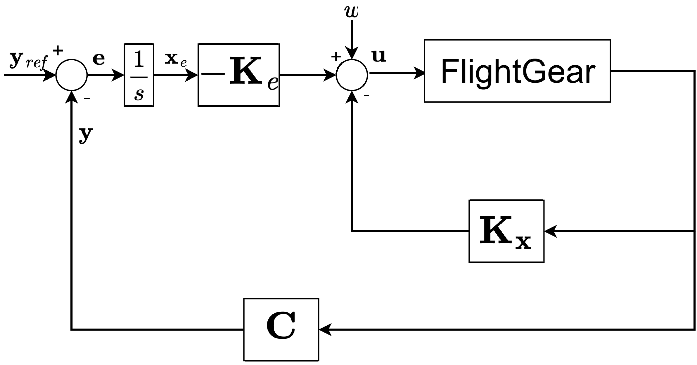
A closed-loop configuration.

3.2 RS-LQR control structure
Structure of an RS-LQR for yaw control.

Figure 4 illustrates the structure of an RS-LQR [Reference Lavretsky and Wise29]. In this section, the RS-LQR controller is designed to track the reference commands for the sideslip angle (
 $\beta$
) and yaw angle (
 $\psi$
) while maintaining satisfactory performance under external disturbances. Unlike a conventional LQR design, which typically relies on heuristically chosen fixed weighting matrices, the proposed RS-LQR approach systematically adjusts the weighting matrices to satisfy prescribed robustness and performance criteria. The RS-LQR controller in this study is designed to regulate only the yaw-axis. For fixed-wing DEP aircraft such as the NASA X-57 Maxwell, differential thrust alone provides control authority mainly in the yaw axis. Therefore, considering the differential-thrust-only FTC framework presented in Section 4, the controller focuses on yaw-axis regulation. The pitch axis is not considered because the longitudinal and lateral dynamics are modelled separately. In the hybrid control scheme, aerodynamic inputs and electric propulsion are combined. Thus, the yaw and roll axes can be directly influenced through the aileron and rudder, and roll can also be indirectly affected through sideslip tracking even when only differential thrust is used (see Equations (3)–(8)). It is assumed that pitch and roll stabilisation are handled by conventional aerodynamic control systems, while the proposed controller is integrated into the overall flight control architecture as a yaw-axis regulator.
In RS-LQR, the error
 $\mathbf{e}$
between the output and the reference is added to the state variables, and the augmented state-space equation is represented as shown in Equation (11):
 \begin{align} &\dot {\mathbf{z}} = \underbrace { \begin{bmatrix} \mathbf{0}_{2\times 2}\;\;\;\;\; & -\mathbf{C} \\ \mathbf{0}_{33\times 2}\;\;\;\;\; & \mathbf{A} \end{bmatrix} }_{\tilde {\mathbf{A}}} \mathbf{z} + \underbrace { \begin{bmatrix} \mathbf{0}_{2\times 16} \\ \mathbf{B} \end{bmatrix} }_{\tilde {\mathbf{B}}} \boldsymbol{\unicode {x03BC}} + \begin{bmatrix} \mathbf{I}_{2\times 2} \\ \mathbf{0}_{32\times 2} \end{bmatrix} \mathbf{r}, \end{align}
where
 \begin{align} \mathbf{z}^T = [\begin{matrix} \mathbf{e}\;\;\;\;\; & {\dot{\mathbf {x}}} \end{matrix}], \quad \boldsymbol{\unicode {x03BC}} = \dot {\mathbf{u}}, \end{align}
and
 \begin{align} &J = \int _{0}^{\infty }\bigl (\mathbf{z}^T \tilde {\mathbf{Q}}_1 \mathbf{z} + \boldsymbol{\unicode {x03BC}}^T \mathbf{R} \boldsymbol{\unicode {x03BC}}\bigr )\,\mathrm{d}t, \end{align}
 \begin{align} & \boldsymbol{\unicode {x03BC}} = - \mathbf{Kz}, \quad \mathbf{u} = - \mathbf{K} \int _0^t \mathbf{z} \, \mathrm{d}t, \end{align}
 \begin{align} &\mathbf{K} = [ \mathbf{K}_e \quad \mathbf{K}_p ] = \mathbf{R}^{-1}\tilde{\mathbf B}^T\mathbf{P}, \end{align}
 \begin{align} & \mathbf{P}\tilde{\mathbf A} + \tilde{\mathbf A}^T\mathbf{P} + \tilde{\mathbf {Q}}_1 - \mathbf{P}\tilde{\mathbf B}\mathbf{R}^{-1} \tilde{\mathbf B}^T\mathbf{P} = \mathbf{0}. \end{align}
Here,
 $\mathbf{z}$
,
 $\dot{\mathbf {x}}$
and
 $\mathbf{r}$
are the augmented state, the derivative of the original state, and the reference input, respectively. Then, the optimal gain
 $\mathbf{K}$
that minimises the standard LQ objective function in Equation (13) is given by Equation (15), where
 $\mathbf{P}$
is the solution to the algebraic Riccati equation (ARE) described in Equation (16), and
 $\tilde{\mathbf{Q}}_1$
and
 $\mathbf{R}$
are the diagonal weighting matrices for
 $\mathbf{z}$
and
 $\boldsymbol{\unicode {x03BC}}$
. The control gain
 $\mathbf{K}$
can be decomposed into
 $\mathbf{K}_p$
for
 $\mathbf{x}$
and
 $\mathbf{K}_e$
for the integral of
 $\mathbf{e}$
, and it stabilises the closed-loop system according to the standard LQR theory [Reference Lavretsky and Wise29]. The input weight matrix for aerodynamic control inputs is defined as
 $\mathbf{R}_f$
, and that for electric propulsion control inputs as
 $\mathbf{R}_p$
.
In this study, the control gains
 $\mathbf{K}_e$
and
 $\mathbf{K}_p$
are obtained through an iterative weighting-matrix tuning procedure. First, since the focus is on a tracking problem,
 $\tilde {\mathbf{Q}}_{1}$
is defined such that all elements except those associated with the tracking error are set to zero, while
 $\mathbf R$
is a diagonal matrix with diagonal entries
 $r_i$
. Next,
 $\tilde {\mathbf{Q}}_{1}$
and
 $\mathbf{R}$
are iteratively adjusted so that all
 $r_i\mu _i^2$
values (where
 $\mu _i$
is an element of
 $\boldsymbol{\unicode {x03BC}}$
) lie within the range of 0.8 to 1.2, which corresponds to the
 $\tilde {\mathbf{Q}}_{1}-{\mathbf R}$
normalisation process. Based on the resulting
 $\tilde {\mathbf{Q}}_{1}$
and
 $\mathbf{R}$
, the individual weighting elements are finally tuned to satisfy the prescribed control performance objectives. Note that the integral gain
 $\mathbf{K}_e$
is introduced to eliminate steady-state tracking error and is determined through the augmented state formulation of the RS-LQR framework, rather than being tuned independently. Because the system is high-dimensional (
 $\mathbf{x} \in \mathbb{R}^{33 \times 1}$
,
 $\mathbf{u} \in \mathbb{R}^{16 \times 1}$
), this study adopts an iterative tuning approach for
 $\tilde {\mathbf{Q}}_{1}$
and
 $\mathbf{R}$
, instead of computing the control gains from explicitly assigned desired poles. The overall input weight matrix is then formulated as follows:
 \begin{equation} \mathbf{R} = \begin{bmatrix} \eta \,\mathbf{R}_f\;\;\;\;\; & \mathbf{0}_{2\times 14}\\ \mathbf{0}_{14\times 2}\;\;\;\;\; & \mathbf{R}_p \end{bmatrix}\!, \end{equation}
where
 $\eta$
denotes a tuning parameter for the hybrid control design to be discussed in the next section.
In addition, in the hybrid yaw control scenario, the yawing moment ratio
 $N_{\text{ratio}}$
, which quantifies the contribution of aerodynamic and electric propulsion forces, is computed as defined in Equation (18):
 \begin{equation} N_{\text{ratio}} =\frac {\left | N_{\mathrm{aero}} \right |} {\left | N_{\mathrm{thrust}} \right |} =\frac {\left | \big (C_{n_{\delta _a}}\,\delta _a + C_{n_{\delta _r}}\,\delta _r\big )\, \bar {q}\,S\,\textit {b} \right |} {\left | \displaystyle \sum _{i=1}^{14} y_{T,i}\,F_{T,i} \right |}. \end{equation}
Here,
 $\bar {q}$
,
 $S$
and
 $\textit {b}$
represent dynamic pressure, wing area and wing span, respectively. Also,
 $C_{n_{\delta _a}}$
and
 $C_{n_{\delta _r}}$
denote the aerodynamic coefficients or yawing effectiveness parameters for
 $\delta _a$
and
 $\delta _r$
, respectively. Together with system response performance metrics such as the settling time
 $T_s$
and maximum overshoot
 $M_p$
,
 $N_{\text{ratio}}$
is used to explore an appropriate trade-off point with respect to the robustness index
 $\alpha ^*$
.
Remark 2. Note that although both the proposed RS-LQR controller and a conventional LQI (linear-quadratic-integral) controller are based on optimal control theory and incorporate integral action to eliminate steady-state tracking errors, their design objectives and tuning methodologies are fundamentally different. In a conventional LQI design, the controller is typically obtained by augmenting the system with integral states and applying a standard LQR formulation with fixed weighting matrices
 $\tilde {\mathbf{Q}}_{1}$
and
 $\mathbf{R}$
, which are generally selected heuristically and remain unchanged throughout the design process. As a result, the controller mainly focuses on balancing tracking performance and control effort without explicitly enforcing robustness criteria, often leading to a trial-and-error tuning procedure. In contrast, the proposed RS-LQR approach extends the conventional LQI framework by explicitly incorporating robustness considerations into the controller synthesis. Specifically, the RS-LQR method is formulated as a robust servomechanism problem in which both tracking performance and robustness against uncertainties are treated as primary design objectives, and the weighting matrices are systematically and iteratively adjusted according to normalisation and performance requirements. This robustness-oriented tuning strategy constitutes a key distinction between the proposed RS-LQR method and a conventional LQI controller.
3.3 Aero-electric hybrid control design and simulation
(a)
 $\alpha ^*$
for different values of
 $N_{ratio}$
; (b) settling times, maximum overshoots and
 $\alpha ^*$
for various
 $\eta$
.

Figure 5 illustrates how the robustness metric
 $\alpha ^*$
and the performance indices vary with the tuning parameter
 $\eta$
. As shown in Figure 5(a),
 $\alpha ^*$
increases with
 $N_{ratio}$
. Figure 5(b) shows that both the settling time (
 $T_s$
) and the maximum overshoot (
 $M_p$
) increase as
 $\eta$
increases. The conventional powered-yaw control based only on electric thrust (e.g. [Reference Kou, Wang and Liang9]) has very low robustness with
 $\alpha ^* \approx 0.002$
. This value is about 250 times smaller than that of the proposed hybrid approach (
 $\alpha ^* = 0.5$
).
State responses and reference-comparison results for the powered-yaw and hybrid-yaw control cases: (a) sideslip and yaw angles; (b) roll rate; (c) yaw rate; (d) roll angle; (e) thrust response of the 1st propulsor (cruise); (f) thrust response of the 2nd propulsor (high-lift); (g) yaw response under hybrid-yaw control for
 $\psi _{\mathrm{ref}}=30^\circ$
; (h) yaw response under powered-yaw control for
 $\psi _{\mathrm{ref}}=30^\circ$
[Reference Kou, Wang and Liang9].

Remark 3. The proposed hybrid-powered yaw controller is developed and evaluated around a representative cruise-flight trim condition, and the tuning parameter
 $\eta$
is therefore selected as a fixed value for that operating point to provide a consistent basis for performance and robustness evaluation. Although this fixed weighting strategy is suitable for the trim-condition-based framework considered in the present study, the balance between aerodynamic and electric propulsion control authority may vary significantly across different flight phases due to changes in dynamic pressure and control effectiveness. Accordingly, future work will investigate gain-scheduling, adaptive control and reinforcement-learning-based strategies for dynamically adjusting
 $\eta$
over a wider flight envelope.
All main results in this study are obtained using a yaw-angle reference of
 $10^\circ$
to satisfy the small-angle assumption. Under this condition, the powered-yaw control has a settling time of about
 $59.5\,\mathrm{s}$
and an overshoot of
 $13.76\%$
. The hybrid-yaw control reduces these values to
 $8.73\,\mathrm{s}$
and
 $3.25\%$
, corresponding to improvements of about
 $85\%$
and
 $76\%$
. With a command filter (a simple low-pass filter for gradually changing the command from 0 to
 $10^\circ$
), the settling time remains similar (
 $8.72\,\mathrm{s}$
). The overshoot is further reduced to
 $1.45\%$
, corresponding to an additional improvement of about
 $55\%$
. Without the command filter, large transient inputs may drive the system beyond the small disturbance region. This violates the linearisation assumptions and degrades control performance.
Figure 6(a) to (f) show the responses of the hybrid-yaw controller for a
 $10^\circ$
yaw command. Figure 6(g) to (h) show the hybrid-yaw control and powered-yaw results from Reference [Reference Kou, Wang and Liang9] with a
 $30^\circ$
reference. For comparison with Reference [Reference Kou, Wang and Liang9], the hybrid-yaw control is also tested at
 $30^\circ$
by temporarily relaxing the linearity condition. The results (Figure 7) are similar to those of the
 $10^\circ$
case. These results show that the hybrid-yaw control improves both robustness and performance. This improvement is achieved by utilising aerodynamic inputs. It also maintains the system within the small-disturbance region, including roll angle and angular rates (
 $p$
,
 $r$
), despite relatively large stability and control derivatives (
 $L_\beta = 8.4455$
,
 $L_{\delta _a} = 19.8557$
,
 $N_{\delta _r} = -4.3696$
). Further, as depicted in Figure 8, the eigenvalue locations of the open-loop and closed-loop systems are compared. In the open-loop case, some eigenvalues of
 $\tilde {\mathbf{A}}$
are located at the origin or in the right half-plane (RHP). This indicates that the open-loop system is unstable. When hybrid-yaw control is applied, all eigenvalues of
 $\tilde {\mathbf{A}} - \tilde {\mathbf{B}}\mathbf{K}$
move into the left half-plane (LHP). This indicates that the closed-loop system becomes asymptotically stable.
Control responses for the powered-yaw and hybrid-yaw control cases: (a) aileron; (b) rudder; (c) thrust command of the 1st propulsor (cruise); (d) thrust command of the 2nd propulsor (high-lift).

Eigenvalues of open-loop vs closed-loop systems.

As depicted in Figure 9, an input multiplicative uncertainty is introduced into the system. Including this input uncertainty, Figure 10 illustrates the responses of the yaw angle at varying levels
 $w$
of the input uncertainty for the hybrid and electric-thrust-only approaches, with the normalised uncertainty
 $\bar{{\varDelta}}$
set to
 $-1$
. When
 $\textit {w} = 0.25$
and
 $\textit {w} = 0.5$
, both control approaches lead to convergence of the desired yaw angle (
 $15^{\circ }$
). However, the electric-thrust-only approach exhibits significantly slower convergence. For a higher level of uncertainty,
 $\textit {w} = 0.75$
, the hybrid approach still demonstrates robustness by maintaining convergence. In contrast, the electric-thrust-only approach fails to converge, and the yaw angle diverges. This divergence is also observed in all state variables and control inputs. These results confirm that the hybrid approach is more suitable than the existing one in terms of improving both performance and robustness.
Input uncertainty inserted into the RS-LQR structure.

Comparison of yaw angle responses after applying the aero-electric hybrid control under different levels (
 $w$
) of input uncertainty: (a)
 $w = 0$
; (b)
 $w=0.25$
; (c)
 $w=0.5$
; (d)
 $w=0.75$
.

4.0 RS-LQR-based FTC design
In the previous section, a hybrid control design combining aerodynamic and electric thrust forces is proposed to improve the robustness to uncertainties in the system. In this section, another robust control design (FTC) is considered to smoothly respond to abrupt and progressive faults in the electric propulsors of aircraft. This FTC consists mainly of three steps: yawing moment equalisation, real-time fault detection and control reconfiguration.
4.1 FTC algorithm with sudden engine failure
4.1.1 Step 1. Fault modelling for electric propulsors
In this study, sudden (complete) faults in electric propulsors are modelled mathematically. For the control input matrix
 $\mathbf{B}_p$
of the electric propulsors, all elements in the columns corresponding to the failed propulsors are set to zero. This fault model represents abrupt and complete propulsor failures, where the corresponding control effectiveness is lost instantaneously. Therefore, setting the corresponding columns of the control input matrix to zero provides a simple and standard representation of actuator loss in the state-space framework. For example, when the 1st and 14th propulsors fail, the fault model can be expressed as in Equation (19):
 \begin{equation} \mathbf{B}_p = \begin{bmatrix} 0\;\;\;\;\; & 0\;\;\;\;\; & \cdots\;\;\;\;\; & 0\;\;\;\;\; & 0 \\ \omega _{F,c}^2\;\;\;\;\; & 0\;\;\;\;\; & \cdots\;\;\;\;\; & 0\;\;\;\;\; & 0 \\ 0\;\;\;\;\; & 0\;\;\;\;\; & \cdots\;\;\;\;\; & 0\;\;\;\;\; & 0 \\ 0\;\;\;\;\; & \omega _{F,h}^2\;\;\;\;\; & \cdots\;\;\;\;\; & 0\;\;\;\;\; & 0 \\ \vdots\;\;\;\;\; & \vdots\;\;\;\;\; & \ddots\;\;\;\;\; & \vdots\;\;\;\;\; & \vdots \\ 0\;\;\;\;\; & 0\;\;\;\;\; & \cdots\;\;\;\;\; & 0\;\;\;\;\; & 0 \\ 0\;\;\;\;\; & 0\;\;\;\;\; & \cdots\;\;\;\;\; & \omega _{F,h}^2\;\;\;\;\; & 0 \\ 0\;\;\;\;\; & 0\;\;\;\;\; & \cdots\;\;\;\;\; & 0\;\;\;\;\; & 0 \\ 0\;\;\;\;\; & 0\;\;\;\;\; & \cdots\;\;\;\;\; & 0\;\;\;\;\; & \omega _{F,c}^2 \end{bmatrix} \quad \Rightarrow \quad \mathbf{B}_{p,\mathrm{fault}} = \begin{bmatrix} 0\;\;\;\;\; & 0\;\;\;\;\; & \cdots\;\;\;\;\; & 0\;\;\;\;\; & 0 \\ 0\;\;\;\;\; & 0\;\;\;\;\; & \cdots\;\;\;\;\; & 0\;\;\;\;\; & 0 \\ 0\;\;\;\;\; & 0\;\;\;\;\; & \cdots\;\;\;\;\; & 0\;\;\;\;\; & 0 \\ 0\;\;\;\;\; & \omega _{F,h}^2\;\;\;\;\; & \cdots\;\;\;\;\; & 0\;\;\;\;\; & 0 \\ \vdots\;\;\;\;\; & \vdots\;\;\;\;\; & \ddots\;\;\;\;\; & \vdots\;\;\;\;\; & \vdots \\ 0\;\;\;\;\; & 0\;\;\;\;\; & \cdots\;\;\;\;\; & 0\;\;\;\;\; & 0 \\ 0\;\;\;\;\; & 0\;\;\;\;\; & \cdots\;\;\;\;\; & \omega _{F,h}^2\;\;\;\;\; & 0 \\ 0\;\;\;\;\; & 0\;\;\;\;\; & \cdots\;\;\;\;\; & 0\;\;\;\;\; & 0 \\ 0\;\;\;\;\; & 0\;\;\;\;\; & \cdots\;\;\;\;\; & 0\;\;\;\;\; & 0 \end{bmatrix}\!. \end{equation}
Note that progressive degradation is treated separately using a time-varying engine-health model, as discussed in the following subsection.
4.1.2 Step 2. Yawing moment equalisation of propulsors
To minimise the effect of a sudden change in the electric thrust due to its failure, the proposed FTC is initially designed such that the yawing moments produced by all propulsors are equalised. In other words, the total yawing moment required at each time instant is equally distributed over the available propulsors. This approach prevents a failure in any single propulsor from excessively affecting the total yawing moment, especially when that propulsor has a larger contribution than the others. As a result, the negative impact on the overall system performance can be reduced. To this end, the LQ performance index Equation (13) is modified as follows:
 \begin{equation} J = \int _0^\infty \big( \mathbf{z}^T \tilde {\mathbf{Q}}_1 \mathbf{z} + \gamma \, \mathbf{z}^T \tilde {\mathbf{Q}}_2 \mathbf{z} + \boldsymbol{\unicode {x03BC}}^T \mathbf{R} \boldsymbol{\unicode {x03BC}} \big) \mathrm{d}t, \end{equation}
where
 $\mathbf{z}^T \tilde {\mathbf{Q}}_2 \mathbf{z}$
measures how uneven the yawing moments are across
 $m$
propulsors by summing the pairwise differences, and mathematically
 \begin{equation} \mathbf{z}^T \tilde {\mathbf{Q}}_2 \mathbf{z} = \sum _{i=1}^{m-1} \sum _{j=i+1}^{m} (y_{T,i} F_{T,i} - y_{T,j} F_{T,j})^2 \end{equation}
with
 \begin{equation} \tilde {\mathbf{Q}}_2= \begin{bmatrix} (m-1) y_{T,1}^2\;\;\;\;\; & -y_{T,1} y_{T,2}\;\;\;\;\; & \cdots\;\;\;\;\; & -y_{T,1} y_{T,m-1}\;\;\;\;\; & -y_{T,1} y_{T,m} \\ -y_{T,2} y_{T,1}\;\;\;\;\; & (m-1) y_{T,2}^2\;\;\;\;\; & \cdots\;\;\;\;\; & -y_{T,2} y_{T,m-1}\;\;\;\;\; & -y_{T,2} y_{T,m} \\ \vdots\;\;\;\;\; & \vdots\;\;\;\;\; & \ddots\;\;\;\;\; & \vdots\;\;\;\;\; & \vdots \\ -y_{T,m-1} y_{T,1}\;\;\;\;\; & -y_{T,m-1} y_{T,2}\;\;\;\;\; & \cdots\;\;\;\;\; & (m-1) y_{T,m-1}^2\;\;\;\;\; & -y_{T,m-1} y_{T,m} \\ -y_{T,m} y_{T,1}\;\;\;\;\; & -y_{T,m} y_{T,2}\;\;\;\;\; & \cdots\;\;\;\;\; & -y_{T,m} y_{T,m-1}\;\;\;\;\; & (m-1) y_{T,m}^2 \end{bmatrix}\!. \end{equation}
The constant
 $\gamma$
in Equation (20) is the yawing moment equalisation factor. A larger
 $\gamma$
reduces the disparity in yawing moments among the propulsors.
4.1.3 Step 3. Real-time fault detection
To detect a sudden fault in the electric propulsors, a real-time fault detection algorithm is proposed as in Table 3. First, the thrust information of each electric propulsor is obtained in real time. The yawing moment
 $\textit {N}_{prop,i}\,(i=1,\ldots ,m)$
is then calculated by multiplying the thrust
 $\textit {F}_{T,i}$
by the moment arm
 $\textit {y}_{T,i}$
. Next, the median value
 $\textit {N}_{med}$
of the
 $m$
yawing moments is computed. The median is used instead of the average to prevent abnormal thrust values from affecting the detection result. Such abnormal values may be excessively low or high because of a propulsor fault. By using the median, the influence of these outliers can be minimised. If the difference between
 $\textit {N}_{prop,i}$
and
 $\textit {N}_{med}$
exceeds a predefined threshold, or if the thrust of any propulsor becomes zero, the corresponding propulsor is considered to have failed. Note that it is assumed to have at most
 $m/2-1$
(or
 $\lceil m/2 \rceil$
for odd
 $m$
) faulty propulsors out of
 $m$
, so that the proposed median-based fault detection approach works.
Real-time electric propulsor fault detection

Table 3. Long description
An equation describing a fault detection algorithm. The algorithm takes electric propulsor thrust F T J and current time t as inputs and outputs a fault detection result is Fault. Preset constants include moment arm tau I, acceptable limit N accept, and simulation time t sim. The algorithm assumes at most m divided by 2 minus 1 faulty propulsors out of m. The while loop runs while t is less than or equal to t sim. For each propulsor, the yawing moment N prop J is calculated as the product of moment arm tau I and thrust F T J. The median of the yawing moments is computed. For each propulsor, if the absolute difference between N prop J and the median N prop med is greater than N accept or if the thrust F T J is zero, the propulsor is marked as faulty. Otherwise, it is marked as not faulty.
Remark 4. Disturbance-induced asymmetric thrust commands must be distinguished from actual propulsor faults. External disturbances, such as wind gusts, can temporarily produce asymmetric thrust distributions. These responses are coordinated across multiple propulsors and remain transient, since the controller drives the system back toward the trim condition. In contrast, a propulsor fault manifests as a persistent and localised deviation in the yawing-moment contribution of a single propulsor. The proposed median-based detection scheme exploits this fundamental difference. Because the median is inherently robust to outliers, a faulty propulsor can be identified as a sustained deviation from the median value. Disturbance-induced control actions generally do not produce persistent outliers, allowing the proposed method to distinguish transient disturbance responses from genuine hardware faults. Furthermore, disturbance-induced deviations are typically short-lived and return to the nominal range as the controller stabilises the system, making it unlikely that they consistently exceed the detection threshold. Conversely, a faulty propulsor generates a sustained deviation that more reliably satisfies the threshold-based fault detection condition. Also, note that, as stated in Remark5 (Section 4.2), online health monitoring schemes can be employed to detect propulsor failures.
4.1.4 Step 4. Control reconfiguration
Once a faulty propulsor is detected, the RS-LQR control proposed in Section 3 is reconfigured to minimise the effect of the faulty propulsor on the system performance. To this end, if the
 $i$
-th electric propulsor fails, the
 $i$
-th column of
 $\mathbf{B}_p$
is replaced with the zero vector. This defines a faulty version of
 $\mathbf{B}_p$
, denoted as
 $\mathbf{B}_{P,\text{fault}}$
, and the corresponding
 $\tilde {\mathbf{B}}_{\text{fault}}$
. Then, the state feedback control gain in Equation (15) is recalculated with
 $\tilde {\mathbf{B}}_{\text{fault}}$
in place of
 $\tilde {\mathbf{B}}$
. This recalculation is based on Equation (16), where
 $\tilde {\mathbf{B}}_{\text{fault}}$
and
 $\tilde {\mathbf{Q}}_1 + \gamma \tilde {\mathbf{Q}}_2$
are used in place of
 $\tilde {\mathbf{B}}$
and
 $\tilde {\mathbf{Q}}_1$
, respectively.
Yawing responses with and without the proposed FTC for a four-engine fault condition: (a) yaw rate; (b) yaw angle; (c) yaw angle response from reference [Reference Kou, Wang and Liang9] (two-engine fault case).

To test the proposed FTC design, a MATLAB simulation was conducted to evaluate the aforementioned steps. In this scenario, the 1st, 2nd, 13th and 14th electric propulsors of the NASA X-57 Maxwell aircraft fail at 2.5 s during the yawing motion. These four propulsors are located near the tips of the left and right wings, where thrust loss has the largest impact on yaw dynamics. Figure 11(a) and (b) show the yawing responses of the aircraft to a step command of 10 degrees. The solid line in each figure represents the case without FTC. The red dashed line represents the case with FTC applied at
 $\gamma =0$
, and the green dash-dotted line represents the case with FTC applied at
 $\gamma =0.01$
. As shown in Figure 11(a) and (b), the yawing responses without FTC diverge after the propulsor fault. When FTC is applied, the aircraft attitude converges stably. In the case of
 $\gamma =0.01$
, where the electric propulsors generate nearly equal yawing moments, the state responses vary more gradually than in the case of
 $\gamma =0$
. This indicates that the effect of propulsor failure is reduced by yawing moment equalisation. Reference [Reference Kou, Wang and Liang9] presents a simulation scenario, shown in Figure 11(c), in which the No. 1 and No. 2 propulsors of the X-57 aircraft fail during a trimmed state. Without FTC, the system fails to return to its original trimmed condition and exhibits a large overshoot. In contrast, the proposed FTC enables the system to converge to the desired yaw angle while maintaining stability under electric propulsion failure.
A sensitivity analysis is conducted to justify the selection of the yawing-moment equalisation factor
 $\gamma$
. The value of
 $\gamma$
is varied over a prescribed range. The level of yawing-moment equalisation among the propulsors is then evaluated using the dispersion metric
 $e_2$
, defined as
 \begin{equation} e_2(\gamma ) = \sum _{i=1}^{13} \sum _{j=i+1}^{14} \left ( \int _{0}^{t_f} [N_{T,i}(t;\;\gamma )-N_{T,j}(t;\;\gamma)]^2 dt \right )^{1/2}, \end{equation}
where
 $i$
and
 $j$
denote the indices of individual propulsors. The term
 $N_{T,i}(t;\;\gamma )$
represents the yawing-moment contribution of the
 $i$
-th propulsor for a given
 $\gamma$
. This metric represents the
 $L_2$
norm of the pairwise yawing-moment differences over time. If a propulsor fault is detected, the corresponding propulsor index is excluded from the summation in Equation (23). A smaller value of
 $e_2(\gamma )$
indicates better equalisation among the propulsors. In the baseline case
 $\gamma = 0$
, the metric value is
 $e_2(0) = 8.2520 \times 10^3$
. For clarity, the metric is normalised with respect to the baseline case as
 \begin{equation} \bar e_2(\gamma )=\frac {e_2(\gamma )}{e_2(0)}, \end{equation}
so that
 $\bar e_2 = 1$
corresponds to the case without equalisation. Figure 12 shows
 $\bar e_2$
as a function of
 $\gamma$
. As
 $\gamma$
increases from zero,
 $\bar e_2$
decreases rapidly, indicating improved equalisation. However, for
 $\gamma \ge 0.01$
, the metric becomes nearly constant. This shows that further increases in
 $\gamma$
provide little additional benefit. These results indicate that most of the equalisation effect is achieved at small values of
 $\gamma$
. Therefore, larger values such as
 $\gamma = 0.5$
do not provide meaningful additional improvement, although they still yield similar qualitative behaviour observed in the previous simulations.
Normalised dispersion metric
 $\bar e_2$
as a function of the yawing-moment equalisation factor
 $\gamma$
.

In addition to the nominal thrust condition, the performance of the proposed active FTC algorithm is evaluated under a realistic thrust measurement environment. This environment includes time delay, constant bias and white noise. The time delay is defined as
 $0.1 \times (1/(\zeta _f \omega _f))$
for each electric propulsor, corresponding to
 $0.0323\,\mathrm{s}$
and
 $0.0024\,\mathrm{s}$
for the cruise and high-lift propulsors, respectively. For each propulsor, an independent random constant bias and bounded noise are applied, and their magnitudes are limited to 5% of the predefined scale values, which are set to 10 for the cruise propulsors and 5 for the high-lift propulsors. This disturbance structure is intended to emulate practical thrust measurement conditions, where the thrust signal first experiences delay through the measurement path and is subsequently corrupted by sensor bias and measurement noise. Note that different bias and noise sequences are independently applied to each propulsor, resulting in asymmetric thrust measurement errors across the propulsion system.
Table 4 presents a comparison of FTC performance between the nominal and realistic thrust measurement conditions. For
 $\gamma = 0$
,
 $0.005$
and
 $0.01$
, the yaw-angle tracking performance is evaluated in terms of settling time and maximum overshoot. Here,
 $\gamma$
denotes the weighting parameter used in the RS-LQR design to adjust the yawing-moment distribution among the propulsors.
 $T_{s,\psi }^{\mathrm{nom}}$
and
 $M_{p,\psi }^{\mathrm{nom}}$
denote the yaw-angle settling time and maximum overshoot under the nominal thrust condition, respectively.
 $T_{s,\psi }^{\mathrm{mean}}$
and
 $M_{p,\psi }^{\mathrm{mean}}$
denote the mean values of the yaw-angle settling time and maximum overshoot obtained from 100 Monte Carlo simulations under the realistic thrust measurement condition.
 $T_{s,\psi }^{\mathrm{diff}}$
and
 $M_{p,\psi }^{\mathrm{diff}}$
represent the relative differences between the nominal result and the Monte Carlo mean result, and are calculated as
 \begin{equation} T_{s,\psi }^{\mathrm{diff}} = \left | \frac {T_{s,\psi }^{\mathrm{mean}}-T_{s,\psi }^{\mathrm{nom}}} {T_{s,\psi }^{\mathrm{nom}}} \right |\times 100, \qquad M_{p,\psi }^{\mathrm{diff}} = \left | \frac {M_{p,\psi }^{\mathrm{mean}}-M_{p,\psi }^{\mathrm{nom}}} {M_{p,\psi }^{\mathrm{nom}}} \right |\times 100. \end{equation}
The results show that the relative settling-time error is less than
 $0.03\%$
, and the maximum overshoot error is less than
 $0.5\%$
for all tested
 $\gamma$
values. Although the errors for
 $\gamma =0.005$
and
 $\gamma =0.01$
are slightly larger than that for
 $\gamma =0$
, the overall degradation remains very limited. This tendency can be attributed to the increased contribution of the high-lift propulsors to yawing-moment generation as
 $\gamma$
increases. Since the high-lift propulsors are more numerous and each propulsor has independent measurement uncertainty, more independent error components can contribute to the yaw response. Nevertheless, the proposed active FTC algorithm maintains robust performance under the considered propulsor-wise thrust measurement uncertainty. In addition, the median-based fault detection algorithm remains reliable under the considered measurement uncertainties, demonstrating robustness against bias, noise and delay.
4.2 FTC algorithm with gradually degraded engine health
In this subsection, the proposed FTC framework is extended to account for progressively degraded engine health. Unlike conventional approaches that assume only abrupt failures, the present study models gradual performance degradation of electric propulsors using a time-varying health parameter
 $\lambda _i(t)$
. Here,
 $\lambda _i(t)$
denotes the remaining effectiveness of the
 $i$
th electric propulsor, where
 $\lambda _i=1$
corresponds to the nominal healthy condition and
 $\lambda _i=0$
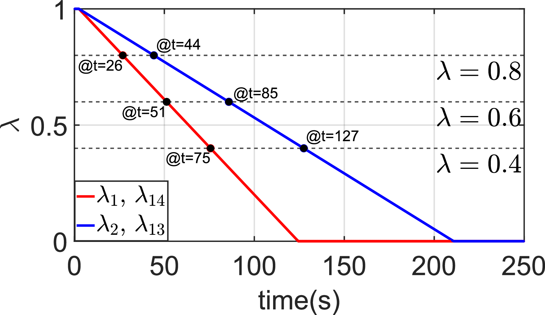
represents a complete loss of thrust effectiveness. Figure 13 illustrates the temporal evolution of the engine health parameters, where different degradation rates are assigned to cruise and high-lift propulsors. The health parameter decreases in a piecewise-linear manner, and the propulsor health condition is classified into four regions using threshold values of
 $\lambda = 0.8$
,
 $0.6$
, and
 $0.4$
. Specifically, the healthy region is defined as
 $0.8 \leq \lambda _i \leq 1$
, indicating that the propulsor retains most of its nominal thrust effectiveness. Type 1 degradation is defined as
 $0.6 \leq \lambda _i \lt 0.8$
and represents a mild loss of effectiveness. Type 2 degradation is defined as
 $0.4 \leq \lambda _i \lt 0.6$
, corresponding to a moderate degradation level in which the reduction in control authority becomes more noticeable. Type 3 degradation is defined as
 $\lambda _i \lt 0.4$
and represents severe degradation or near-failure conditions. These four health regions provide the basis for the gain-switching logic, and the corresponding RS-LQR gain set is selected according to the current value of
 $\lambda _i(t)$
. These time-varying health states are directly incorporated into the control input matrix through the modified matrix
 $\mathbf{B}_{p,\text{fault}}$
, where the
 $i$
th column of
 $\mathbf{B}_{p,\text{fault}}$
is multiplied by the corresponding health parameter
 $\lambda _i(t)$
. This formulation enables the controller to explicitly account for changes in actuator effectiveness as the degradation progresses.
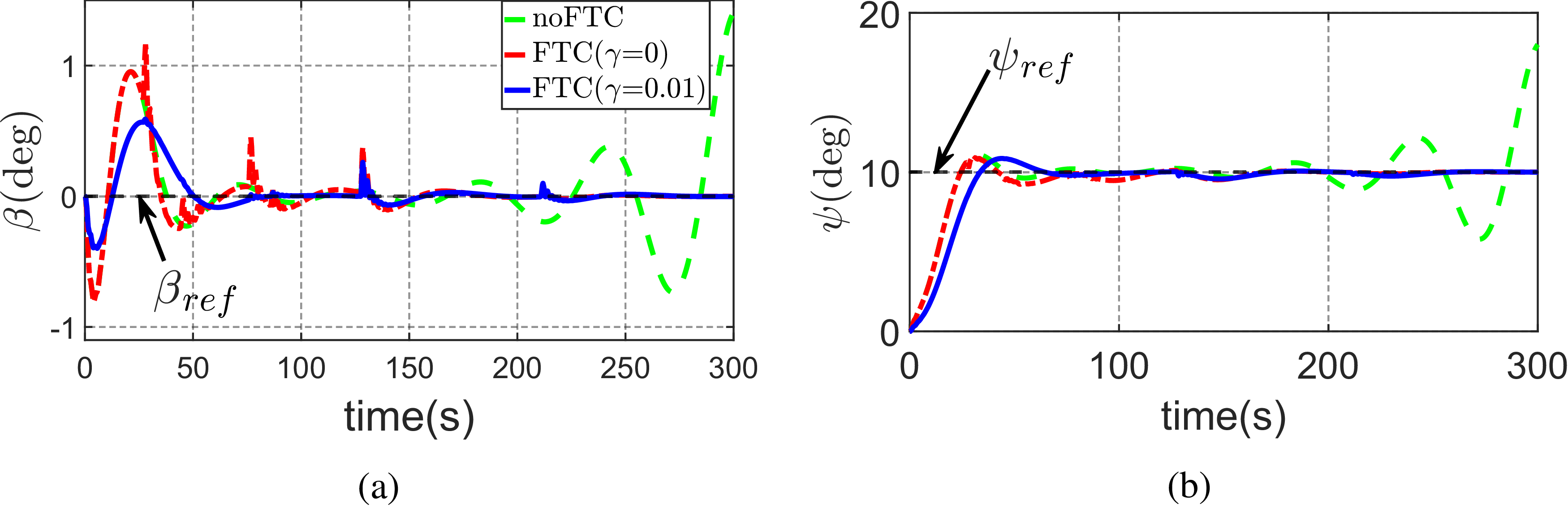
As a result, the control allocation accounts for the real-time degradation level of each propulsor rather than relying only on binary fault conditions. Furthermore, since the proposed RS-LQR framework employs gain switching based on the predefined health regions, the control gains are updated discretely according to the system health state. As the degradation progresses across the thresholds, multiple gain switchings occur, enabling the controller to maintain stability and tracking performance throughout the degradation process. Figure 14 presents the responses of the sideslip angle (
 $\beta$
) and yaw angle (
 $\psi$
) under gradually degraded engine health conditions. Without FTC, the system exhibits increasing oscillations and eventually diverges as degradation progresses. In contrast, the proposed FTC method maintains stable and accurate tracking performance. In particular, the case with
 $\gamma =0.01$
shows the most robust response under progressive degradation. These results demonstrate that the proposed FTC framework can handle both gradual degradation and complete failure within a unified control structure.
Comparison of FTC performance under nominal and realistic thrust conditions

Table 4. Long description
A table comparing FTC performance under nominal and realistic thrust conditions. The table has 4 rows and 7 columns. Column headers are: , , , , , , . Row 1: , 0, 59.4431, 9.0571, 9.0636, 0.0033, 0.0070. Row 2: , 0.005, 67.6157, 8.4284, 8.4691, 0.0256, 0.4820. Row 3: , 0.01, 67.6356, 8.4274, 8.4687, 0.0272, 0.4905.
Gradually degraded engine health modelling.

Sideslip and yaw angle responses with gradually degraded engine health: (a) sideslip angle response; (b) yaw angle response.

Hughes H4 Hercules model in FlightGear.

Remark 5. It is important to note that the degradation profile
 $\lambda _i(t)$
is assumed to be available from an external propulsion health-monitoring or fault-diagnosis system. This assumption is consistent with recent studies on DEP, electric-propulsion and multirotor aircraft health monitoring. Online rotor-health monitoring studies have shown that rotor faults can be detected, identified and quantified using in-flight strain measurements, and that rotor degradation values can be estimated with confidence intervals [Reference Dutta, Niemiec, Gandhi and Kopsaftopoulos30, Reference Dutta, Niemiec, Kopsaftopoulos and Gandhi31]. Electric aircraft powertrain diagnosis studies have also demonstrated that faults in critical propulsion subsystems, such as motors and electronic speed controllers, can be detected and isolated in a distributed manner [Reference Kulkarni, Roychoudhury and Gorospe32]. Furthermore, recent work on electric-propulsion aircraft has shown that propeller faults can be diagnosed using motor-electric signals without requiring additional sensors [Reference Lee, Kim, Noh, Jeong, Kong and Yoo33]. These results indicate that the remaining propulsor effectiveness required in the present FTC framework does not need to be prescribed a priori; instead, the fault magnitude or health information estimated by such monitoring algorithms can be converted into
 $\hat {\lambda }_i(t)$
and supplied to the modified input matrix
 $\mathbf{B}_{\text{p, fault}}$
.
5.0 Verification of the DEP controller using flight simulator
In this section, the proposed controller is validated using a widely used flight simulator, FlightGear [34]. FlightGear is an open-source flight simulation platform that supports simulations of various types of aircraft [Reference Kim and Kim35] and is freely available. Note that the NASA X-57 Maxwell was adopted in the earlier sections of the study because its configuration and publicly available aerodynamic data provide an appropriate reference platform for developing the aircraft dynamic equations and control framework. However, the purpose of the FlightGear validation in this section is not to reproduce the exact aerodynamic behaviour of the X-57, but rather to verify the correct implementation of the proposed nonlinear 6-DOF dynamics and control architecture within a realistic flight simulation environment. For this purpose, the Hughes H4 Hercules model (Figure 15) available in the FlightGear–JSBSim environment was selected because JSBSim employs the same fundamental nonlinear rigid-body flight dynamics equations used in the theoretical formulation. In addition, the H4 model provides dynamically consistent aerodynamic coefficients, inertial properties and actuator models, enabling realistic closed-loop interaction between the controller and the simulated aircraft.
Although the H4 Hercules differs from the X-57 in geometry, propulsion configuration and actuator characteristics, these differences do not affect the primary objective of the validation, which is to confirm the correct integration of the controller, simulator interface and nonlinear aircraft dynamics framework. The controller interacts with the simulator through standard control inputs that are translated by JSBSim into aerodynamic forces and moments, meaning that aircraft-specific parameters mainly influence quantitative responses rather than the correctness of the implementation itself. Therefore, the FlightGear experiments should be interpreted as validation of the simulation and control framework, not as aerodynamic validation of the X-57 aircraft or its distributed electric propulsion system. The study demonstrates successful implementation of the nonlinear 6-DOF equations, stable closed-loop behaviour and proper controller–simulator interaction within the FlightGear–JSBSim environment, while acknowledging that aircraft-specific X-57 validation remains future work.
5.1 Development of a co-simulation environment integrating FlightGear and MATLAB
The control verification begins with the development of a co-simulation environment for integrating FlightGear (aircraft) with MATLAB (the proposed control). Fortunately, FlightGear supports various network communication protocols, including TCP/IP, UDP and Serial for interfacing with external programmes such as MATLAB [36]. In this study, UDP-based communication is employed due to its high transmission speed, making it suitable for real-time applications, despite its inherent drawback of potential data loss [Reference Kurose and Ross37]. This UDP-based FlightGear-MATLAB integration follows a structured process, consisting of the following key steps.
5.1.1 Implementation of the generic protocol [36, 38]
Generic protocol for UDP-based co-simulation.

To enable UDP communication between FlightGear and external programmes, the generic protocol must be implemented, as illustrated in Figure 16. FlightGear’s generic protocol provides a flexible method for exchanging data in either ASCII-based or binary format by defining an XML-encoded configuration file and placing it in the FG_ROOT/Protocol/ directory. This protocol operates by continuously reading data in a loop until no more usable data is available, ensuring that each iteration maintains the most up-to-date data state. This mechanism is particularly useful when the sender transmits data at a higher rate or when FlightGear experiences delays, as it prevents data loss and ensures real-time processing. The generic protocol consists of three main components: input node – defines the structure of incoming data; output node – specifies the format of outgoing data; and chunk node – configures data attributes, including property tree structure, data type and format. To identify the necessary input and output data nodes, users can utilise the FlightGear Property Tree Browser, which allows inspection of the internal property tree structure and selection of relevant data fields for generic protocol configuration [39].
5.1.2 Batch file [Reference Aschauer, Schirrer and Kozek40, Reference Sagliano41]
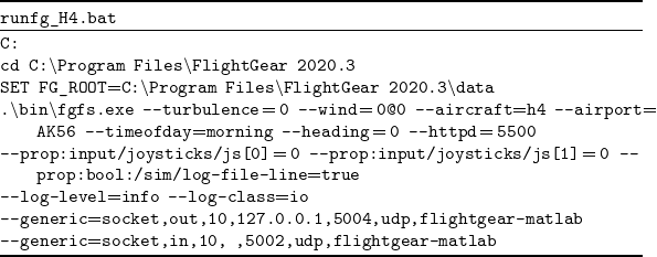
To run FlightGear with the implemented generic protocol from MATLAB, a batch file must be created as shown in Table 5. When writing the batch file, make sure that everything from .∖bin∖fgfs.exe onward is written on a single line.
Batch file for co-simulation with generic protocol

Table 5. Long description
The image displays a batch file script named runfg_H4.bat. The script sets the root directory for FlightGear 2020.3 and configures various simulation parameters. It includes settings for turbulence, wind, aircraft type, airport, time of day, heading, and HTTP server port. Additionally, it configures joystick inputs, logging options, and generic socket connections for communication with MATLAB. The script specifies UDP protocols and ports for data exchange.
5.1.3 MATLAB/simulink
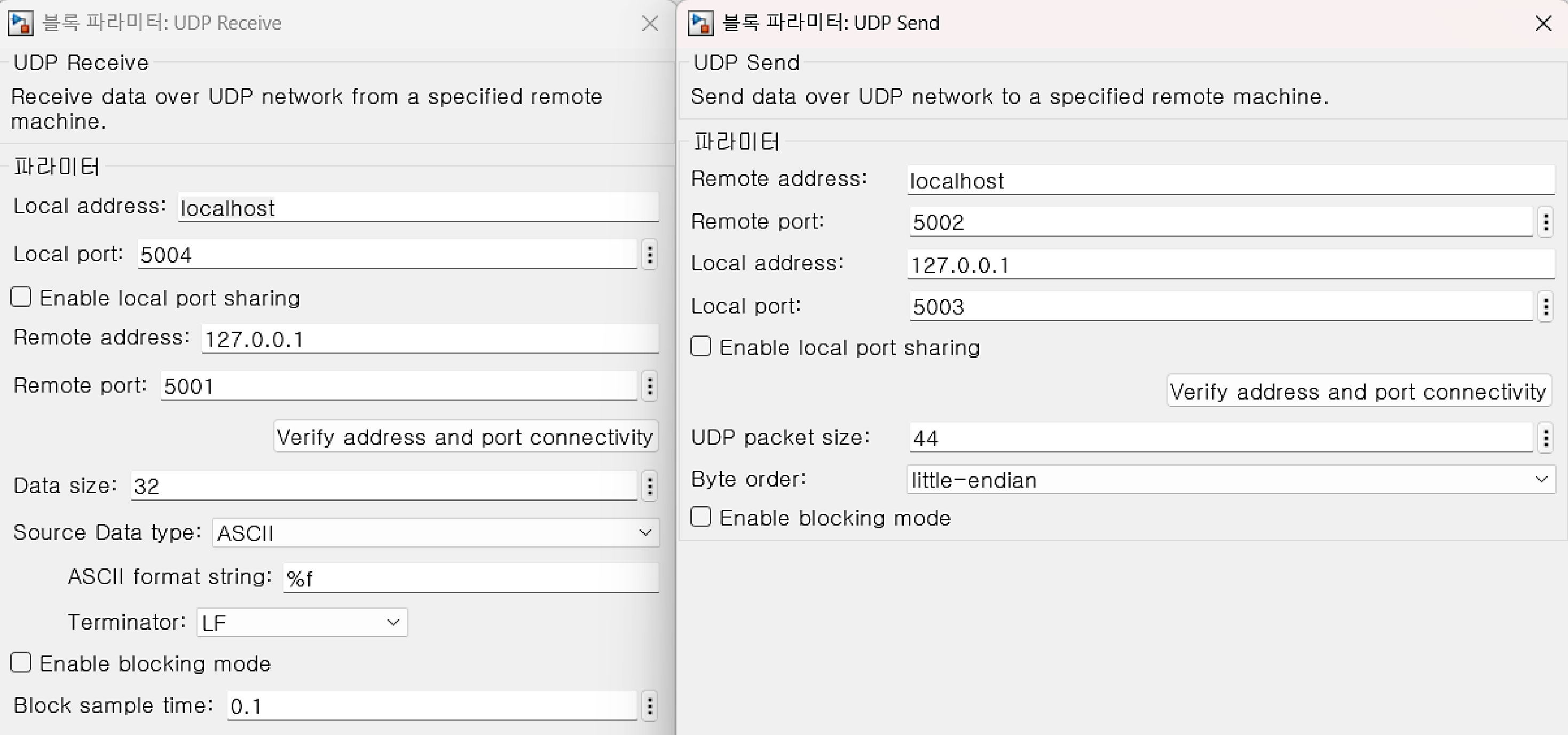
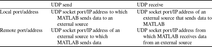
UDP send and receive block parameters.

The UDP-based co-simulation between MATLAB and FlightGear is then implemented using the UDP Send and UDP Receive blocks in MATLAB/Simulink. The UDP Send block is used to transmit UDP data from MATLAB to an external programme, while the UDP Receive block is used to receive UDP data from an external programme [43, 44]. Figure 17 shows the parameter settings for the UDP Send and UDP Receive blocks. Descriptions of the Local port/address and Remote port/address settings are provided in Table 6.
Description of local port/address and remote port/address

Table 6. Long description
A table with two rows and two columns comparing UDP send and receive port/address configurations in MATLAB. The columns are labeled ‘UDP send’ and ‘UDP receive’. The rows are labeled ‘Local port/address’ and ‘Remote port/address’. Row 1: Local port/address, UDP socket port/IP address to which MATLAB sends data to an external source, UDP socket port/IP address of an external source that sends data to MATLAB. Row 2: Remote port/address, UDP socket port/IP address of an external source to which MATLAB sends data, UDP socket port/IP address from which MATLAB receives data from an external source.
Hybrid-powered yaw control using the RS-LQR structure for the aircraft model in FlightGear.

Remark 6. Note that UDP-based communication is widely used in co-simulation frameworks involving MATLAB/Simulink and flight simulators such as FlightGear because of its low latency and suitability for real-time data exchange [Reference Aschauer, Schirrer and Kozek40, Reference Horri and Pietraszko42]. Although UDP does not guarantee packet delivery, stable co-simulation can be achieved in controlled local network environments. In this study, data exchange between MATLAB and FlightGear is implemented using the generic protocol with a transport update rate of 10 Hz, which provides a practical balance between communication load and real-time responsiveness. The generic protocol continuously reads incoming data and uses the most recent available values, even when packets are delayed. This sample-and-hold-like update mechanism reduces the impact of occasional packet loss on the closed-loop system. All simulations are conducted in a controlled local network environment, where packet loss and latency are negligible. Therefore, their impact on closed-loop performance is limited. Nevertheless, because UDP does not ensure reliable data delivery, more advanced communication strategies, such as packet loss mitigation and fault-tolerant network architectures, remain important topics for future work.
5.2 System identification for aircraft model
Flight state responses for LQR control (solid) and no control (dashed): (a) sideslip angle and yaw angle; (b) roll rate; (c) yaw rate; (d) roll angle; (e) four engines’ thrust forces on the left wing; (f) four engines’ thrust forces on the right wing.

Flight control inputs for LQR control: (a) aileron; (b) rudder; (c) four engines’ throttle inputs on the left wing; (d) four engines’ throttle inputs on the right wing.

For the control design described in Section 3, a system model of the target aircraft is required. To this end, a standard procedure of system identification is performed for the Hughes H4 Hercules aircraft model in FlightGear, primarily due to the lack of aerodynamic data and moment-of-inertia information needed for deriving the dynamic equations. Rather than using a black-box identification approach, which relies only on input–output and model-order information, a grey-box identification approach is employed to estimate the structured system matrices
 $\mathbf{A}_{F}$
,
 $\mathbf{A}_{PF}$
,
 $\mathbf{A}_{P}$
,
 $\mathbf{B}_{F}$
, and
 $\mathbf{B}_{P}$
in Equation (8), based on a known dynamic model structure [Reference Yu, Ljung and Verhaegen45]. This approach enables the derivation of physically meaningful dynamics necessary for the hybrid powered yaw control discussed in the following section. Based on the identified system model, the transfer functions from
 $\delta _a$
to
 $p$
(roll rate) and from
 $\delta _r$
to
 $r$
(yaw rate) can be approximated as second-order transfer functions:
 \begin{equation} \begin{aligned} G_{\delta _a}^{\,p}(s)&=\frac {407.7\,s+5020}{s^2+73.39\,s+280.5}, \quad G_{\delta _r}^{\,r}(s)&=\frac {0.3373\,s+4.962}{s^2+0.8345\,s+2.795}. \end{aligned} \end{equation}
Note that these transfer functions are used for initially taking the aircraft to a trim condition via simple PI (proportional-integral) controllers, before verifying the hybrid powered yaw control. In fact, the PI gain values for
 $G_{\delta _a}^p$
are
 $K_p^{roll} = 0.002866$
and
 $K_i^{roll}= 0.1327$
, while those for
 $G_{\delta _r}^r$
are
 $K_p^{yaw} = 0.1205$
and
 $K_i^{yaw}= 0.3692$
. The lateral-directional state-space equations of the H4 Hercules obtained using the grey-box model identification method are given as Equation (27), where
 $\kappa _1$
 $\sim$
 $\kappa _4$
in the matrix
 $\mathbf{A}_{PF}$
are
 $1.2968\times 10^{-6}$
,
 $9.8833\times 10^{-7}$
,
 $6.8348\times 10^{-7}$
and
 $3.7347\times 10^{-7}$
, respectively.
 \begin{equation} \mathbf A = \begin{bmatrix} \mathbf A_F\;\;\;\;\; & \mathbf A_{PF}\\[2pt] \mathbf 0_{8\times 5}\;\;\;\;\; & \mathbf A_P \end{bmatrix}\!, \quad \mathbf B = \begin{bmatrix} \mathbf B_F\;\;\;\;\; & \mathbf 0_{5\times 8}\\[2pt] \mathbf 0_{8\times 2}\;\;\;\;\; & \mathbf B_P \end{bmatrix}\!, \quad \text{with} \end{equation}
 \begin{equation} \mathbf A_F= \begin{bmatrix} -0.4523\;\;\;\;\; & -0.0600\;\;\;\;\; & -0.8710\;\;\;\;\; & 0.0934\;\;\;\;\; & -0.0136\\ -1.4046\;\;\;\;\; & -3.9030\;\;\;\;\; & 0.7010\;\;\;\;\; & -0.0317\;\;\;\;\; & -0.0013\\ 2.1325\;\;\;\;\; & -0.1351\;\;\;\;\; & -0.9012\;\;\;\;\; & -0.0044\;\;\;\;\; & -0.0051\\ 0.0099\;\;\;\;\; & 1\;\;\;\;\; & -0.0177\;\;\;\;\; & -9.6755\times 10^{-4}\;\;\;\;\; & -0.0071\\ 0.0332\;\;\;\;\; & 0.0098\;\;\;\;\; & 1\;\;\;\;\; & -0.0058\;\;\;\;\; & 0.0141 \end{bmatrix}\!, \quad \mathbf A_P=-9.2509\,\mathbf I_8, \end{equation}
 \begin{equation} \mathbf A_{PF}= \begin{bmatrix} \;\;\;\;\; & \;\;\;\;\; & \;\;\;\;\; & \;\;\;\;\; & {\mathbf 0_{1\times 8}}\;\;\;\;\; & \;\;\;\;\; & \;\;\;\;\; & \\\;\;\;\;\; & \;\;\;\;\; & \;\;\;\;\; & \;\;\;\;\; & {\mathbf 0_{1\times 8}}\;\;\;\;\; & \;\;\;\;\; & \;\;\;\;\; & \\ \kappa _1\;\;\;\;\; & \kappa _2\;\;\;\;\; & \kappa _3\;\;\;\;\; & \kappa _4\;\;\;\;\; & -\kappa _4\;\;\;\;\; & -\kappa _3\;\;\;\;\; & -\kappa _2\;\;\;\;\; & -\kappa _1\\ \;\;\;\;\; & \;\;\;\;\; & \;\;\;\;\; & \;\;\;\;\; & {\mathbf 0_{1\times 8}}\;\;\;\;\; & \;\;\;\;\; & \;\;\;\;\; & \\ \;\;\;\;\; & \;\;\;\;\; & \;\;\;\;\; & \;\;\;\;\; & {\mathbf 0_{1\times 8}}\;\;\;\;\; & \;\;\;\;\; & \;\;\;\;\; & \end{bmatrix}\!, \quad \mathbf B_F= \begin{bmatrix} 0.0106\;\;\;\;\; & -0.0324\\ 1.2152\;\;\;\;\; & -0.0800\\ 0.0569\;\;\;\;\; & 0.2840\\ -0.0021\;\;\;\;\; & 0.0012\\ -0.0042\;\;\;\;\; & -3.0774\times 10^{-4} \end{bmatrix}\!, \end{equation}
 \begin{equation} \mathbf B_P=57838.9\,\mathbf I_8. \end{equation}
5.3 Hybrid-powered yaw control verification
5.3.1 Software-in-the-loop simulation (SILS)
As depicted in Figure 18, the identified aircraft model from Section 5.2 is integrated into the RS-LQR control structure. The LQR control (i.e.
 $\mathbf{K}_e = 0$
) is first designed and evaluated to verify whether the aircraft successfully returns to the trim condition when the state is perturbed. To simulate an off-trim condition in FlightGear, an aileron step input is applied for the first 2 s. Then, after 10 s, the LQR controller is activated to observe whether all state variables return to the trim condition. Figure 19 presents the responses of the system with and without the LQR controller when the aircraft deviates from the trim state, while Figure 20 illustrates the control inputs. A state variable approaching zero indicates that the aircraft has returned to the trim state. Overall, the system with LQR control, using both aerodynamic and electric forces, successfully returns to the trim condition within 200 s, whereas the system without the LQR controller diverges. However, a steady-state error remains because the LQR controller cannot fully compensate for uncertainties and disturbances during flight.
The hybrid-powered yaw control for general tracking is then designed and tested. Following the design procedure described in Section 3.2, the control gains
 $\mathbf{K}_x$
and
 $\mathbf{K}_e$
are obtained to drive the aircraft yaw angle to
 $10$
degrees. Figures 21 and 22 show the state variables and control inputs after applying the control gains. As observed in both figures, all state variables and control inputs converge within approximately 80 to 100 s through the combined use of aerodynamic and electric control forces. These results confirm that the sideslip angle and yaw angle successfully reach the desired targets within 80 s. Note that, due to technical issues in implementing engine faults in FlightGear, the proposed FTC design in Section 4 could not be validated under thrust-loss scenarios.
Flight state responses for the hybrid-powered yaw control (SILS): (a) sideslip and yaw angles; (b) roll rate; (c) yaw rate; (d) roll angle; (e) four engines’ thrust forces on the left wing; (f) four engines’ thrust forces on the right wing.

Flight control inputs for the hybrid-powered yaw control (SILS): (a) aileron; (b) rudder; (c) four engines’ throttle inputs on the left wing; (d) four engines’ throttle inputs on the right wing.

5.3.2 Hardware-in-the-loop simulation (HILS)
Raspberry Pi-based HILS workspace for hybrid yaw control verification.

Flight state responses for the hybrid-powered yaw control (HILS): (a) sideslip and yaw angles; (b) roll rate; (c) yaw rate; (d) roll angle; (e) four engines’ thrust forces on the left wing; (f) four engines’ thrust forces on the right wing.

Flight control inputs for the hybrid-powered yaw control (HILS): (a) aileron; (b) rudder; (c) four engines’ throttle inputs on the left wing; (d) four engines’ throttle inputs on the right wing.

This section briefly presents the results of the HILS. In this simulation, the MATLAB controller used in the SILS described in Section 5.3.1 is replaced with Raspberry Pi hardware to control the H4 Hercules aircraft. The Raspberry Pi-based HILS workspace is shown in Figure 23. It consists of three main components: the FlightGear simulator, the Raspberry Pi hardware and a display module for verifying data transmission and reception. The same control gains used in the SILS are applied, and the simulation is conducted under the same trim conditions for the lateral state variables and control inputs. As shown in Figures 24 and 25, the HILS results closely match those obtained in Section 5.3.1. This demonstrates that all state variables and control inputs converge stably and effectively.
Remark 7. Containerised execution environments, such as Docker-based deployment on Raspberry Pi hardware, represent a promising direction for improving determinism, reproducibility and implementation-level robustness in future real-time flight-control systems. However, such implementation-oriented enhancements are beyond the scope of the present study and are therefore identified as meaningful future work.
6.0 Conclusion and future work
This paper proposed hybrid-powered yaw control and FTC strategies for DEP aircraft within an RS-LQR framework. The hybrid controller significantly improved yaw tracking performance, reducing the settling time from
 $59.5$
to
 $8.73\,\mathrm{s}$
and the maximum overshoot from
 $13.76\%$
to
 $3.25\%$
. The effectiveness of the proposed approach was validated through MATLAB–FlightGear co-simulation and Raspberry Pi-based HILS, where consistent results were obtained.
Future work will focus on developing a DEP aircraft model in FlightGear for FTC validation under thrust-loss conditions, extending the proposed control framework to nonlinear models, and improving the robustness and determinism of the real-time HILS implementation through advanced communication and deployment architectures. In addition, gain-scheduling or adaptive strategies for dynamically adjusting the tuning parameter
 $\eta$
across different flight conditions will be investigated to enhance practical applicability. Future research will also consider the direct incorporation of engine-health prognostics into the control design framework to enable more realistic health-aware fault-tolerant control and predictive adaptation under gradually degrading propulsion conditions.
Data availability
Additional data supporting the findings of this study are available from the corresponding author upon request.
Acknowledgements
This work was supported by the Glocal University 30 Project Fund of Gyeongsang National University in 2026. The authors used AI-assisted tools during the research and manuscript preparation process in accordance with the journal’s policy and requirements.
Competing interest
All authors have no conflicts of interest, financial or personal, that may have influenced the findings presented in this study.


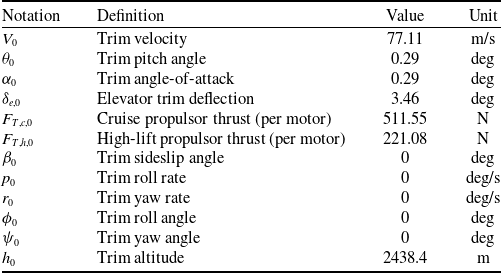

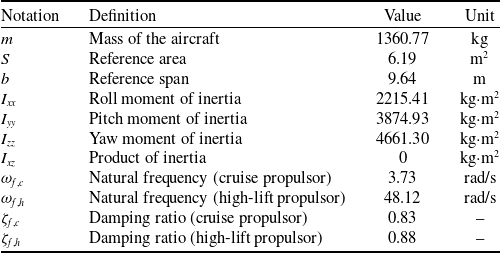
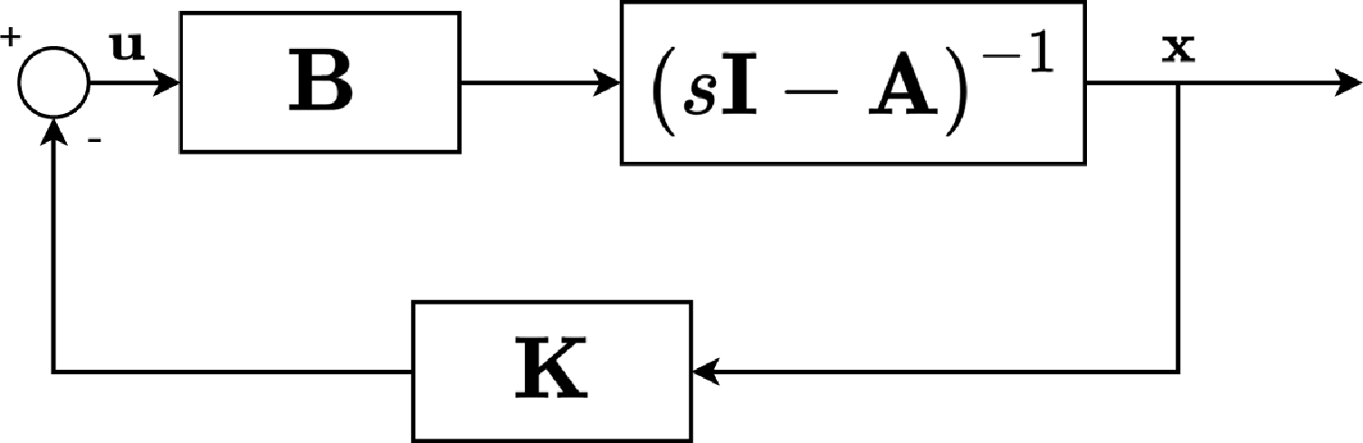
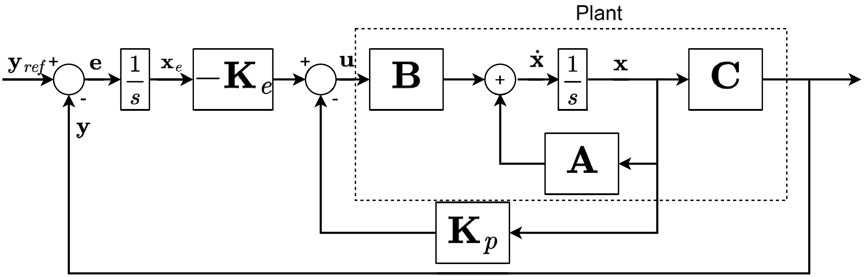
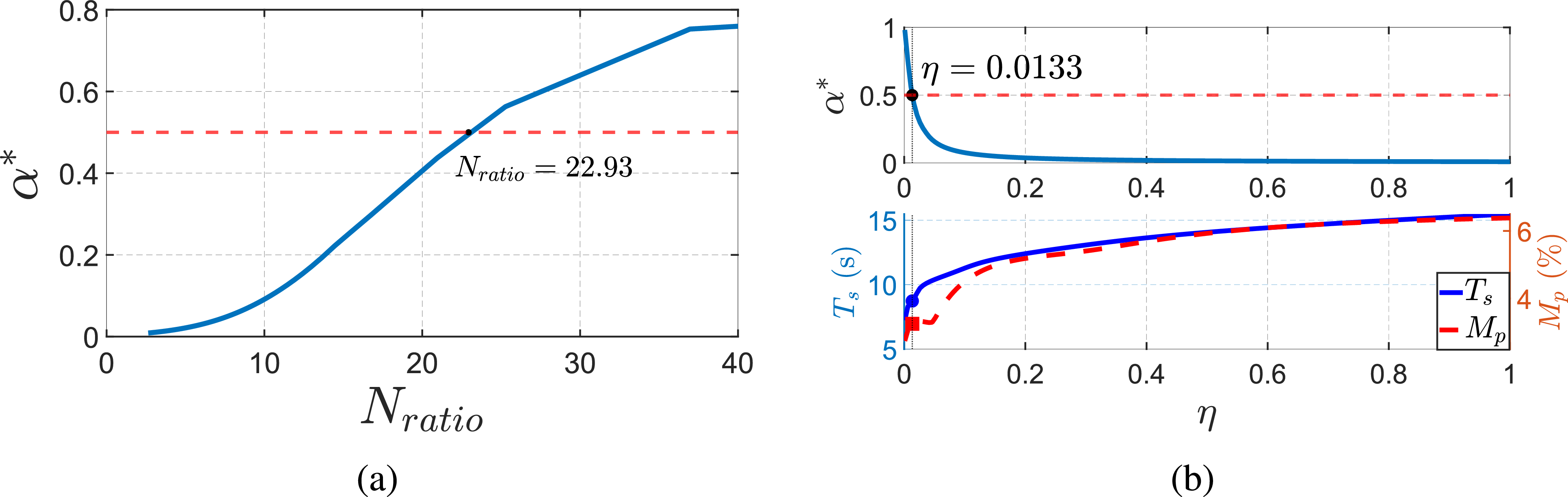
 α∗
 Nratio
 α∗
 η

 ψref=30∘
 ψref=30∘

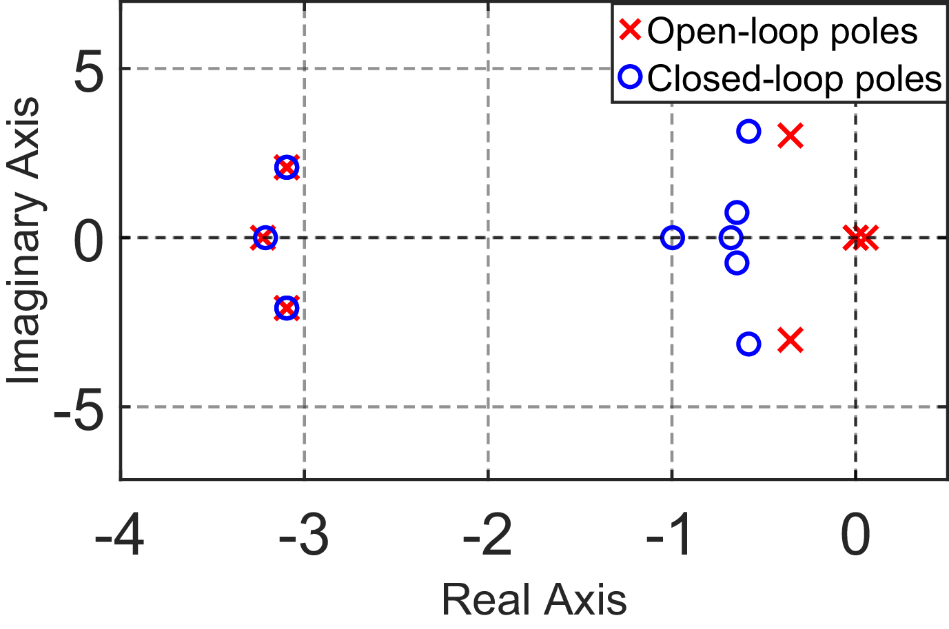
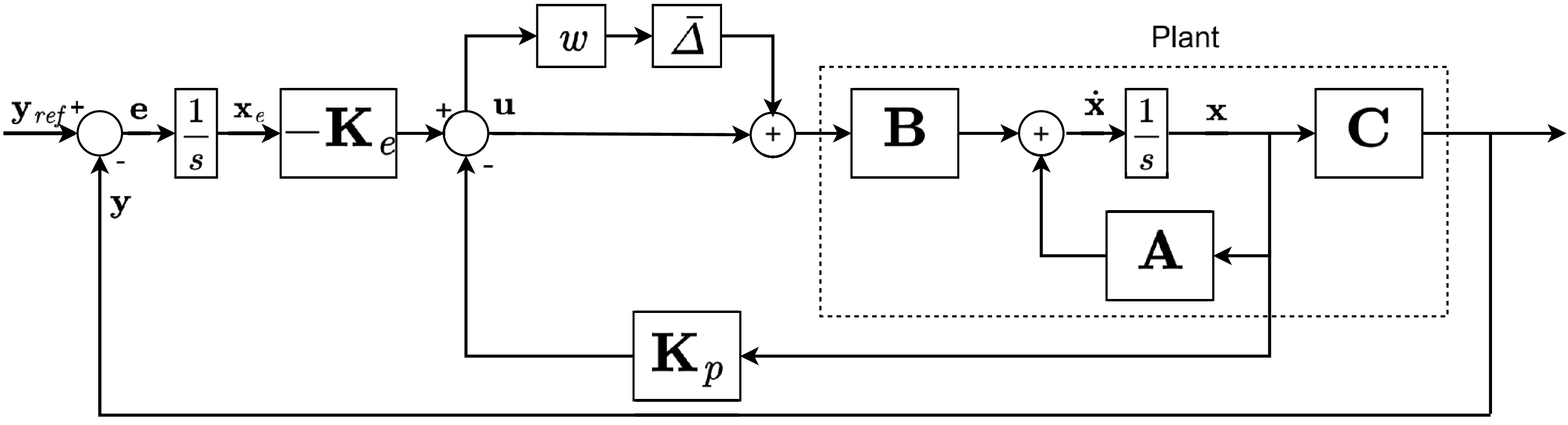

 w
 w=0
 w=0.25
 w=0.5
 w=0.75
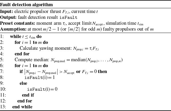

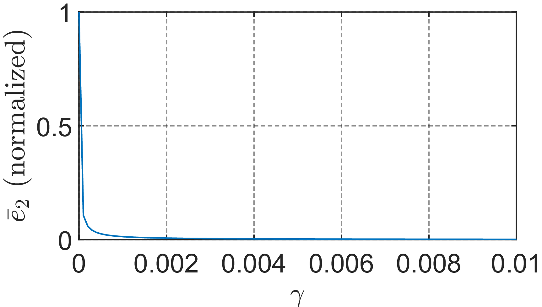
 e¯2
 γ