

NOMENCLATURE
- A
-
coefficient in minimum drag relation
- A(r)
-
quadratic coefficient, Equation (7)
- B
-
number of propeller blades
- B(r)
-
linear coefficient, Equation (7)
- C(r)
-
constant coefficient, Equation (7)
- c(r)
-
local chord
- cd (r)
-
local drag coefficient
- c dmin(r)
-
local sectional minimum drag coefficient
- cl (r)
-
local lift coefficient
- c lmd
-
lift coefficient for minimum sectional drag
- clα (r)
-
sectional lift curve slope
- Cp
-
power coefficient
- CQ
-
torque coefficient
- CT
-
thrust coefficient
- D
-
propeller diameter
- d
-
drag
- F(r)
-
tip loss factor
- J
-
advance ratio
- kp
-
drag due to lift parameter
- K
-
constant
- l
-
lift
- m
-
constant
- n
-
rotation rate
- Q
-
torque
- R
-
propeller radius
- r
-
radial co-ordinate of blade
- T
-
thrust
- V∞
-
freestream velocity
- Vi
-
induced velocity
- ViX (r)
-
axial component of induced velocity
- Viθ (r)
-
tangential component of induced velocity
- w 0
-
displacement velocity of wake vortex sheet
- X(r)
-
location of separation
- α∞ (r)
-
flow angle
- αi (r)
-
induced angle
- αzl
-
aerofoil section zero lift angle-of-attack
- β(r)
-
blade pitch angle
- β tip(r)
-
blade pitch angle at propeller tip
- η
-
propulsive efficiency
- μ
-
viscosity
- ω
-
angular velocity of propeller
- max
-
maximum
- ch
-
chord
Subscripts
1.0 INTRODUCTION
The basic tenets of propeller analysis were developed by Rankine(Reference Rankine1), Froude(Reference Froude2), Glauert(Reference Glauert3), Goldstein(Reference Goldstein4) and Betz(Reference Betz5). Emerging from their efforts were the blade element momentum (BEM) and vortex theories of propeller performance. Both approaches are well validated and have been used extensively for propeller analysis. High-fidelity methods exist (vortex lattice theory(Reference Masquelier6) as well as CFD(Reference Carroll and Marcum7)) to analyse propellers; however, their greater complexity has not led to mainstream use. BEM or vortex theory analysis requires the discretisation of the blade into radial stations. The solution is iterative at each radial station, and usually progresses from the hub to the tip. Iteration is required to establish the effect of the helical wake whose influence is embodied in the axial and tangential induction factors (BEM method) or the induced angle-of-attack (vortex theory). Both approaches usually require an extensive database or look-up table that quantifies the blade section characteristics in terms of lift and drag coefficients as affected by angle-of-attack and Reynolds number. At low advance ratios, significant inner extents of the blade may exhibit separated flow. Flow separation necessitates the implementation of a stall model. Development of a stall model is complicated by blade rotation effects (Coriolis contribution and radial pressure gradients(Reference Breton8)); lift coefficients considerably higher than those seen statically may be realised(Reference Ronsten9). Several semi-empirical stall models exist(Reference Snel, Houwink, van Bussel and Bruining10–Reference Corrigan and Schilling13), however their generality or accuracy for propeller analysis has not been established.
The methods of Lock(Reference Lock14) and Slavik(Reference Slavik15) were developed to simplify propeller analysis and are based on estimation of properties at the r/R = 0.7 blade station. The implementation of these methods still requires a sufficient amount of effort such that any time benefit compared to a BEM implementation may not be significant.
While the basic requirements for designing an optimal propeller were evinced by Betz(Reference Betz5), it was not until 1979 that Larrabee(Reference Larrabee16) codified the requirements into a systematic theory. Propeller optimality requires the helicoidal wake to displace rearwards at a constant velocity. Limitations of Larrabee's method as identified by Adkins and Liebeck(Reference Adkins and Liebeck17) yielded their theory for blade design. Both methods require the specification of a desired thrust or power for a given propeller radius, number of blades and advance ratio. Adkins and Liebeck's(Reference Adkins and Liebeck17) method requires an implementation similar to a BEM code, while the approach of Larrabee is non-iterative but does use small-angle approximations.
It would be useful to have a cohesive non-iterative propeller analysis method that is easy to implement and that can be readily used for design. A stall model and aerofoil data input that mitigates the need for look-up tables of aerofoil characteristics would also be desirable. Consequently, the development of such a methodology is the focus of this paper. The method is based on vortex theory as presented by Phillips(Reference Phillips18). A stall model is developed in conjunction with an approximation of the aerofoil aerodynamics as affected by Reynolds number and angle-of-attack. The theory is then modified to facilitate use as an optimal blade design tool and is readily implementable in any spreadsheet program. Comparisons between theory and experiment are presented for validation.
2.0 THEORETICAL DEVELOPMENT
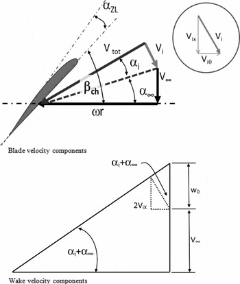
A theory is presented to estimate the induced angle-of-attack along the propeller blade. Subsequently, a simplified representation of the sectional aerodynamics characteristics, including the modelling of stall effects, is introduced. Figure 1 shows a description of the blade geometric and aerodynamic nomenclature. Using Goldstein's vortex theory, Phillips(Reference Phillips18) derived a relation for the induced angle-of-attack along the blade caused by the propeller's wake. Goldstein's theory(Reference Goldstein4) (which assumes the trailing vortex sheet lies along a helical surface of constant pitch) relates the bound circulation on each of the blades at a radius r to the circulation around a stream tube in the wake of radius r (neglecting the wake contraction that occurs with high loading). The circulation around the blade at radial station r (which is dependent on the number of blades, the tip loss factor and the tangential velocity component) can also be found using the Kutta-Joukowski theorem, yielding two expressions for circulation, which can be equated to yield(Reference Phillips18):
 $$\begin{equation}
\frac{{Bc(r)}}{{16r}}{c_l}(r) - F(r)\frac{\pi }{2}{\rm{tan}}[{\alpha _i}(r)]{\rm{sin}}[{\alpha _i}(r) + {\alpha _\infty }(r)] = 0
\end{equation}$$
Blade and wake geometric and aerodynamic nomenclature.

This equation must be solved numerically for the induced angle-of-attack at each discrete radial station. Prandtl's tip loss factor(Reference Phillips18), F(r), is given by:
 $$\begin{equation}
F(r) = \frac{2}{\pi }{\rm{co}}{{\rm{s}}^{ - 1}}\left( {{e^{\frac{{ - B(1 - r/R)}}{{2{\mathop{\rm s}\nolimits} {\rm{in}}{\beta _{{\rm{tip}}}}}}}}} \right)
\end{equation}$$
and represents the fact that a propeller is not a solid disk, but is composed of a finite number of blades. The factor F(r) accounts for the relative velocity of the entrained fluid between the helicoidal sheets and that of the sheets themselves. Note that β tip is the pitch angle at the blade tip measured to the aerofoil's zero lift line. The angle of the resulting flow at radial station r, excluding induced effects is given by:
 $$\begin{equation}
{\alpha _\infty }(r) = {\rm{ta}}{{\rm{n}}^{ - 1}}\left( {\frac{{{V_\infty }}}{{\omega r}}} \right)
\end{equation}$$
The local lift coefficient at any station r along the blade may be calculated using:
 $$\begin{equation}
{c_l}(r) = {c_{l\alpha }}(r)\left[ {{\beta _{\rm ch}}(r) - {\alpha _{zl}} - {\alpha _i}(r) - {\alpha _\infty }(r)} \right]
\end{equation}$$
Using small-angle approximations (implying low to moderate loading) allows Equation (1) to be simplified by expanding sin[α i(r)+α ∞(r)] and approximating tan(α i(r)) ≈ sin(α i(r)) ≈ αi (r) and cos(αi (r)) ≈ 1 to yield:
 $$\begin{equation}
\frac{{Bc(r)}}{{16r}}{c_l}(r) - F(r)\frac{\pi }{2}{\alpha _i}(r)[{\rm{sin}}({\alpha _\infty }(r)) + {\alpha _i}(r){\rm{cos}}({\alpha _\infty }(r))] = 0
\end{equation}$$
Using a small-angle approximation is consistent within the intent of the theoretical development i.e. an easily implementable preliminary analysis code. Substituting Equation (4) for (Reference Betz5) and manipulating into the form of a quadratic equation gives:
 $$\begin{eqnarray}
&&{\alpha _i}{(r)^2}\left[ {F(r)\frac{\pi }{2}{\rm{cos}}({\alpha _\infty }(r))} \right] + {\alpha _i}(r)\left[ {\frac{{Bc(r)}}{{16r}}{c_{l\alpha }}(r) + F(r)\frac{\pi }{2}{\rm{sin}}({\alpha _\infty }(r))} \right] \nonumber\\
&&\quad- \frac{{Bc(r)}}{{16r}}{c_{l\alpha }}(r)[{\beta _{\rm ch}}(r) - {\alpha _\infty }(r) - {\alpha _{zl}}] = 0
\end{eqnarray}$$
i.e. a quadratic in αi . Solving gives:
 $$\begin{equation}
\begin{array}{l} A(r) = F(r)\displaystyle\frac{\pi }{2}{\rm{cos}}({\alpha _\infty }(r))\\[8pt] B(r) = \displaystyle\frac{{Bc(r)}}{{16r}}{c_{l\alpha }}(r) + F(r)\displaystyle\frac{\pi }{2}{\rm{sin}}({\alpha _\infty }(r))\\[8pt] C(r) = - \displaystyle\frac{{Bc(r)}}{{16r}}{c_{l\alpha }}(r)[{\beta _{\rm ch}}(r) - {\alpha _\infty }(r) - {\alpha _{zl}}] \end{array}
\end{equation}$$
such that:
 $$\begin{equation}
{\alpha _i}(r) = \frac{{ - B(r) + \sqrt {B{{(r)}^2} - 4A(r)C(r)} }}{{2A(r)}}
\end{equation}$$
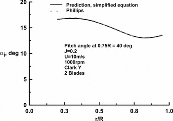
Figure 2 presents a comparison between Equation (8) and numeric solution of Equation (1) for a high-load (CT = 0.12) condition for the propeller defined in Ref. Reference Hartman and Biermann23. As seen, the agreement is essentially exact. The propeller thrust is given by(Reference Phillips18):
 $$\begin{eqnarray}
T &=& \frac{{B\rho {\omega ^2}}}{2}\int_{r = {\rm hub}}^R {{r^2}c(r)\frac{{{\rm{co}}{{\rm{s}}^2}({\alpha _i}(r))}}{{{\rm{co}}{{\rm{s}}^2}({\alpha _\infty }(r))}}} {c_l}(r)\nonumber\\
&& \times\, \left( {{\rm{cos}}[{\alpha _i}(r) + {\alpha _\infty }(r)] - \frac{{{c_d}(r)}}{{{c_l}(r)}}{\rm{sin}}[{\alpha _i}(r) + {\alpha _\infty }(r)]} \right)dr
\end{eqnarray}$$
Effect of small-angle approximation on computed α i .

and the torque by:
 $$\begin{eqnarray}
Q &=& \frac{{B\rho {\omega ^2}}}{2}\int_{r = {\rm{hub}}}^R {{r^3}c(r)\frac{{{\rm{co}}{{\rm{s}}^2}({\alpha _i}(r))}}{{{\rm{co}}{{\rm{s}}^2}({\alpha _\infty }(r))}}} {c_l}(r) \nonumber\\[10pt]
&&\times\, \left( {{\rm{sin}}[{\alpha _i}(r) + {\alpha _\infty }(r)] + \frac{{{c_d}(r)}}{{{c_l}(r)}}{\rm{cos}}[{\alpha _i}(r) + {\alpha _\infty }(r)]} \right)dr
\end{eqnarray}$$
The theoretical development presented can be readily implemented without the need for iteration or an equation solver. Equations (9) and (10) may be evaluated using any numerical integration scheme; e.g. Newton-Cotes quadrature (trapezoidal or preferably Simpson's rule) or Gaussian quadrature.
2.1 Estimation of the sectional lift and drag coefficient
Representative performance estimates are contingent upon accurate determination of cl (r) and cd (r). The difficulty lies in the fact that the inner portions of the blade may be at a very high angle-of-attack (depending on the blade geometry and design advance ratio) – especially at low values of J. Consequently, a stall model may be required.
2.2 Estimation of the lift coefficient
Estimation of the lift coefficient requires an expression that encompasses both the attached and separated flow regimes. The impact of separation may be estimated using the Kirchoff zone of constant pressure formulation(Reference Leishman and Crouse19) in conjunction with a suitable switch function to simulate the forward movement of the line of separation. It is thus implicitly assumed that separation is initiated at the trailing edge and progresses forward. Consequently, the local lift coefficient may be expressed as:
 $$\begin{equation}
{c_l}(r) = {c_{l\alpha }}(r)\left[ {{\beta _{\rm ch}}(r) - {\alpha _{zl}} - {\alpha _i}(r) - {\alpha _\infty }(r)} \right]{\left[ {\frac{{1 + X{{(r)}^m}}}{2}} \right]^2}
\end{equation}$$
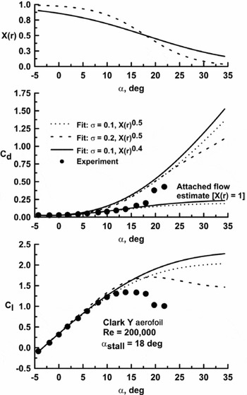
In Equation (11), X(r) represents the location of separation, X(r) = 1 implies fully attached flow and X(r) = 0 implies fully separated flow. In Kirchoff's formulation, m = 0.5, however, it has been left variable such that the effect of m may be explored. To estimate X(r), a function is needed that switches from 1 to 0 at a rate that may be set empirically. An exponential function of the form(Reference Traub20):
 $$\begin{equation}
X(r) = \frac{1}{{1 + {e^{\sigma \left[ {\alpha (r) - {\alpha _{{\rm{stall}}}}} \right]}}}}
\end{equation}$$
is suitable. The parameter σ determines the rate at which the function switches; increasing σ speeds up the transition. The effect of σ and m is explored in Fig. 3; the experimental data is from Reference TraubRef. 21. Increasing σ causes a more rapid forward progression of the stall location such that lift drops more rapidly following stall. Reducing m from 0.5 to 0.4 (for a given σ) slows the movement of separation and consequently delays the onset of lift loss in the stall regime. Consequently, adjustment of the parameter σ in Equation (12) and m in Equation (11) allows a heuristic estimation of blade stall effects as impacted by rotation. A meaningful physical interpretation of σ and m may be attached in their influence on the rate of separation progression. Setting σ = 0.1 and m = 0.4 yields a cl plots similar in form and magnitude to that presented in Ronsten(Reference Ronsten9). Consequently, these values were used in subsequent analysis. As will be shown, they yield accurate modelling at low advance ratios for the presented cases; however, this does not ensure their generality. It should be noted that X(r) may be determined directly using aerofoil data by solving Equation (11) for X(r). In this instance, the first term in brackets on the right-hand side would be replaced by [α − α zl ].
Impact of stall model variables on estimated c l and cd . Experimental data from Reference TraubRef. (21).

2.3 Estimation of the drag coefficient
The drag coefficient can be modelled using a polar representation in the attached flow regime coupled with an estimate once separation manifests. Once large-scale separation occurs, it may be expected that the aerofoil loses leading-edge suction (basically the inviscid axial force). In this case, it would follow that the lift-dependent drag coefficient is given by Cl (r)tan(α(r)) – the stream-wise component of the normal force. Thus the drag coefficient may be expressed as(Reference Traub20):
 $$\begin{eqnarray}
{c_d}(r) &=& X(r)[ {{c_{d{\rm{min}}}}(r) + {k_p}{{\left( {{c_l}(r) - {c_{l{\rm md}}}} \right)}^2}} ] \nonumber\\
&&+\, \left( {1 - X(r)} \right)\left[ {{c_l}(r){\rm{tan}}(\alpha (r)) + 0.5{c_{d{\rm{min}}}}(r){\rm{cos}}({\alpha _{{\rm{geom}}}}(r))} \right]
\end{eqnarray}$$
or approximating c dmin(r) = ARe(r)γ
 $$\begin{eqnarray}
{c_d}(r) &=& X(r)[ {\left( {A{\rm{Re}}{{(r)}^\gamma }} \right) + {k_p}{{\left( {{c_l}(r) - {c_{l{\rm md}}}} \right)}^2}} ] \nonumber\\
&&+\,\left( {1 - X(r)} \right)\left[ {{c_l}(r){\rm{tan}}(\alpha (r)) + 0.5{c_{d{\rm{min}}}}(r){\rm{cos}}({\alpha _{{\rm{geom}}}}(r))} \right]
\end{eqnarray}$$
The first bracketed term on the right-hand side of Equations (13a or 13b) represents the attached flow drag contribution while the second bracketed term represents the separated flow drag. From Fig. 1,
 $$\begin{equation*}
\alpha (r) = {\beta _{\rm ch}}(r) - {\alpha _i}(r) - {\alpha _\infty }(r)
\end{equation*}$$
Comparison with experimental results has shown a small improvement in accuracy at low values of the advance ratio J if the absolute angle-of-attack is used instead of the geometric value i.e.
 $$\begin{equation}
\alpha (r) = {\beta _{\rm ch}}(r) - {\alpha _i}(r) - {\alpha _\infty }(r) - {\alpha _{zl}}
\end{equation}$$
Equation (14) should be used as the estimate of α(r) in Equation (13b)
The Reynolds number is calculated using:
 $$\begin{equation}
{\rm{Re}}(r) = \frac{{\omega r \times {\rm{cos}}({\alpha _i}(r))}}{{{\rm{cos}}({\alpha _\infty }(r))}}\frac{{\rho c(r)}}{\mu }
\end{equation}$$
The minimum drag coefficient (c dmin(r) = ARe(r)γ), drag due to lift (kp ) parameter and cl md need to be estimated. To find A and γ:
-
• Generate data that covers the Re range for the propeller from the hub to the tip. Use 4 or 5 radial stations (e.g. r/R = 0.2, 0.4, 0.6, 0.8 and 0.95). Calculate the Re at each station and then analyse to generate drag polars (cd Vs cl ). The drag polars may be generated experimentally or numerically (Xfoil, Eppler code, CFD, etc). While the generation of an aerodynamic database is required, the aerodynamic model negates the need for interpolation and adds a stall model to the data set.
-
• For each polar find the minimum drag coefficient, cd min(r).
-
• Plot cd min(r) as a function of Re.
-
• Fit a power curve to the data, the coefficient is A and the exponent γ.
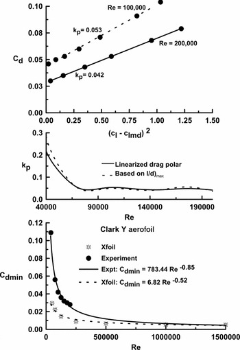
The drag due to lift parameter kp (which relates to the sectional pressure drag) is found through linearisation of the drag polar i.e. plotting cd verse (cl-cl md)2. The slope of the resulting curve is then kp . An example is shown in Fig. 4, top plot. Experimental data from Ref. 21 was used for analysis. Fortuitously, kp does not have a strong dependence on Re(Reference Barlow, Rae and Pope22), unless pressure drag is very high as seen for Re < 100,000, Fig. 4. For simplicity, an alternative approach to finding kp that does not require linearisation and analysis of the resulting polar would be desirable. Writing down the basic expression for the drag polar and dividing by cl gives:
 $$\begin{equation*}
\frac{{{c_d}}}{{{c_l}}} = \frac{{{c_{d{\rm{min}}}}}}{{{c_l}}} + \frac{{{k_p}}}{{{c_l}}}{\left( {{c_l} - {c_{l{\rm{md}}}}} \right)^2}
\end{equation*}$$
Determination of input parameters for aerofoil polar.

Subsequent differentiation of this expression with respect to cl yields:
 $$\begin{equation*}
\frac{{d\left( {\frac{{{c_d}}}{{{c_l}}}} \right)}}{{d{c_l}}} = 0 = \frac{{ - {c_{d{\rm{min}}}}}}{{{c_l}^2}} - \frac{{{k_p}{c_{l{\rm{md}}}}^2}}{{{c_l}^2}} + {k_p} = {c_{d{\rm{min}}}} + {k_p}{c_{l{\rm{md}}}}^2 - {k_p}{c_l}^2
\end{equation*}$$
In this expression, cl is that for l/d)max. Solving for kp gives:
 $$\begin{equation}
{k_p} = \frac{{{c_{d{\rm{min}}}}}}{{{c_{l{{(l/d)}_{{\rm{max}}}}}}^2 - {c_{l{\rm{md}}}}^2}}
\end{equation}$$
This equation (denoted as ‘Based on l/d)max’) is compared with kp estimates based on the slope of the linearised drag polar (middle plot of Fig. 4). As presented, agreement between the two approaches is good.
2.4 Method of solution
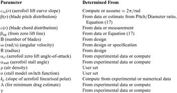
Prior to analysis the following inputs, as shown in Table 1, are required. In some instances, especially if analysing small propellers as are common for R/C aircraft, the pitch distribution is not generally known. While the chord may be easily measured, most manufacturers specify the propellers’ pitch-to-diameter ratio as measured at 75%R. Under the assumption of constant pitch, the blade's pitch distribution may then be estimated as:
 $$\begin{equation}
\beta (r) = {\rm{ta}}{{\rm{n}}^{ - 1}}\left( {\frac{{(P/D)}}{{\pi (r/R)}}} \right)
\end{equation}$$
Required inputs
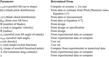
Once the input parameters have been determined, the method proceeds as follows:
-
1. Discretise the blade, starting at the hub, or r/R = 0.05, 0.1 to no less than 0.95R (to model the blade as completely as possible). The equations are evaluated at each r.
-
2. If the blade is variable pitch, the pitch angle can be added to the local blade pitch βch(r) for all r.
-
3. Calculate the tip loss factor, F(r), Equation (2).
-
4. Calculate the angle of the resulting flow excluding induced effects, α ∞(r) Equation (3).
-
5. Calculate the induced angle-of-attack, αi (r), Equations (7) and (8).
-
6. Calculate X(r), Equation (12) and then the local lift coefficient, cl (r), Equation (11).
-
7. Calculate the local Reynolds number, Equation (15).
-
8. Calculate the local drag coefficient, cd (r), Equation (13(b)).
-
9. Evaluate and integrate Equations (9) and (10).
If coefficients are desired, they can be established using:
Thrust coefficient
 $$\begin{equation}
{C_T} = \frac{T}{{\rho {n^2}{D^4}}}
\end{equation}$$
Torque coefficient
 $$\begin{equation}
{C_Q} = \frac{Q}{{\rho {n^2}{D^5}}}
\end{equation}$$
Power coefficient
 $$\begin{equation}
{C_p} = 2\pi {C_Q}
\end{equation}$$
The propeller efficiency can be calculated using
 $$\begin{equation}
\eta = \frac{J}{{2\pi }}\frac{{{C_T}}}{{{C_Q}}}
\end{equation}$$
where the advance ratio is given by:
 $$\begin{equation}
J = \frac{{{V_\infty }}}{{nD}}
\end{equation}$$
and n has units of revolutions per second; D is the propeller diameter.
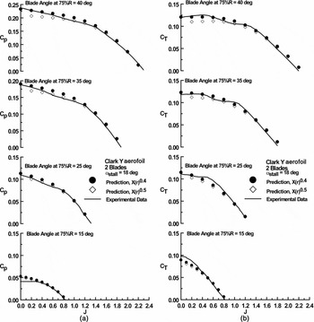
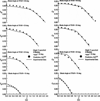
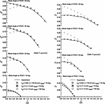
Figures 5(a) and (b) present comparison of the method with experiment. Experimental data from NACA report 640(Reference Hartman and Biermann23) was used for validation. To be consistent with the original NACA data presentation, the experimental data is presented in the form of a line and not explicit data points. The characteristics of the propeller's aerofoil (a Clark Y) were established using XfoilFootnote 1 . The stall angle was set to 18°(Reference Silverstein24) and corresponds to the angle just prior to large-scale lift attenuation. An aerofoil zero lift angle of –5.2° was used. Although this angle appears to differ from Xfoil and current experiment(Reference Traub21) where a value of αzl ≈ –3.2° is estimated, contemporary wind-tunnel data for a Clark Y (Reference Silverstein24) showed αzl = –5.2°. As was common, angles were measured from the lower surface of the Clark Y; the angle between the pressure surface and chord line of this aerofoil is 2°. Thus the angle between the angular measurement reference and the aerofoil's zero lift line is –5.2°. For the tests in Ref. 23 the Reynolds number generally varied from approximately 300,000 to 1.6 × 10⁶. Agreement between experiment and theory for both the power and thrust coefficient is encouraging, Figs 5(a) and (b). The effect of m in Equation (11) is also examined. Increasing m from 0.4 to 0.5 hastens the forward progression of separation, consequently at low J where stall manifests, this decreases the thrust and power coefficient. In subsequent comparisons, m will be set to 0.4 following from the better agreement shown in Fig. 5. Note that the predicted η was not examined as erroneous estimates of CT and Cp can fortuitously yield representative efficiency predictions. Comparisons with a four-bladed propeller are presented in Figs 6(a) and (b). The experimental data is also from NACA Report 640(Reference Hartman and Biermann23). Close agreement between theory and experiment is once again demonstrated. The accord shown in Figs 5 and 6 at low J between theory and experiment suggests that the stall model formulation fits the observed behaviour well. At low J, significant extents of separated flow exist over the inner portions of the blade. Rotational effects yield span-wise and chord-wise (caused by the Coriolis effect) pressure gradients that result in a radial motion of the separated flow, stabilising it and augmenting lift production(Reference Breton8). However, the drag associated with the lift augmenting separated flow still reflects a lack of leading-edge suction causing high required propeller input power.
Comparison of theory and experiment, (a) power and (b) thrust coefficient. Data from Ref. (Reference Hartman and Biermann23).

Comparison of theory and experiment, (a) power and (b) thrust coefficient. Data from Ref. (Reference Hartman and Biermann23).

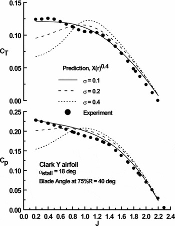
In the present stall model σ affects the rate at which stall progresses from the trailing edge forward. The effects of σ on cl was explored in Fig. 3, however σ’s impact on CT and Cp has not been directly examined, see Fig. 7. Increasing σ yields higher coefficient estimates at high advance ratios where the blade's angle-of-attack is generally low and the flow is attached. At low J, where stall is common over the inboard blade extent, larger values of σ hasten the loss of lift. Low values of σ result in a gradual stall progression that extends over a larger incidence range, see Fig. 3.
Effect of σ on calculated thrust and power coefficient.

The effect of attached flow viscous modelling (reflected in A and kp ) in cd estimation as well as the prescribed αstall is explored in Figs. 8(a) and (b). As seen, viscous modelling has a negligible impact on the calculated thrust and power coefficient; a consequence of the comparatively high blade operational Reynolds number reducing cd min. Eliminating the stall model (i.e. setting αstall = 100°) yields a marked over prediction of thrust at low J, with estimated lift coefficients exceeding 2 over the inboard extents of the blade (not presented). Correspondingly, the required power is greatly underestimated, as the blade shows no drag rise associated with separation (cl tan α).
Effect of viscous parameters on estimate (a) power and (b) thrust coefficient. Data from Ref. (Reference Hartman and Biermann23).

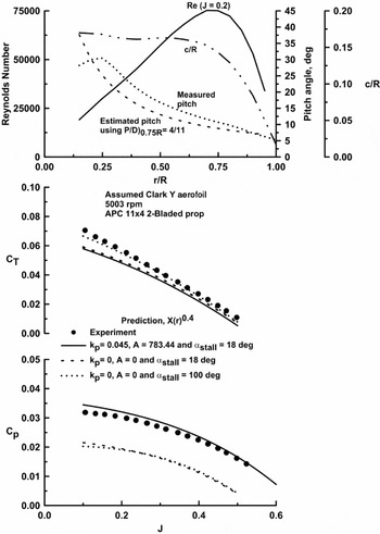
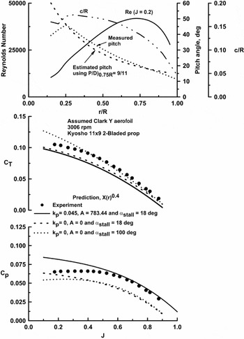
Many small unmanned aerial vehicles use propellers from the hobby R/C sector. A simple method by which the performance of their propellers may be estimated would be of value. Analysis of R/C type propellers is complicated by uncertainty associated with their constituting geometry and their blade section. While the blade's chord may be readily measured, determination of its pitch can be problematic. Figures 9 and 10 show comparison between two typical R/C propellers and current theory. Both of the propellers had 11 in diameters; the APC was low pitch, 11 × 4; while the Kyosho was high pitch, 11 × 9. The experimental data is from Ref. 25. The propellers’ chord and pitch were measured(25), while their performance was determined using a test stand. The top plots in Figs 9 and 10 summarise the propeller's geometry as well as their operational Reynolds number. Most R/C propeller manufacturers specify their products’ pitch-to-diameter ratio at 75%R. Using this value, the pitch distribution was estimated using Equation (17). This pitch distribution was used in performance calculations as it is unlikely that for most initial estimates the pitch distribution of the blade would be known. As the propeller's aerofoil section was not specified, a Clark Y was assumed, such that the data in Fig. 4 was used to estimate its properties. Immediately apparent is the extremely low operational Reynolds number of the propellers. Considering the uncertainty in the inputs, the accord between experiment and theory is reasonable. Unlike the data in Fig. 8; the attached flow viscous contribution of the blade's profile significantly affects the power estimates; a consequence of the low Reynolds number. Also of interest is that even without a stall model (α stall = 100°) CT at low J can often be fortuitously estimated as rotational stall effects can yield high lift coefficient values; similar to those observed if stall modelling is neglected. However, Cp is seen to be greatly underestimated as the drag associated with separation is not simulated.
Comparison of theory and experiment, APC 11 in. by 4 in. propeller. Data from Ref. (25).

Comparison of theory and experiment, Kyosho 11 in by 9 in propeller. Data from Ref. (25).

For a stall model to be considered robust, it should not be case specific. The presented test cases may be considered to represent extremes for application of the presented methodology. They range from full-scale propellers in Reference Hartman and BiermannRef. 23 to that of small R/C propellers (Ref. 25). In both cases the stall parameters that give the best overall agreement with the experiment are the same for both the full-scale and R/C propellers. This suggests that within the range of propellers investigated, the stall model may be considered representative.
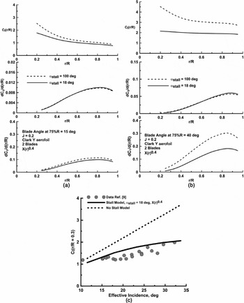
The effect of the stall model on the radial thrust and torque loading is presented in Figs. 11(a) and (b). Two cases are shown for J = 0.2 (blade data from Reference Hartman and BiermannRef. 23); one for a 75% blade angle of 15° (Fig. 11(a)) and the other for a 40° blade angle (Fig. 11(b)). Setting αstall = 100° negates the stall model. Viscous modelling of the drag polar was still included using kp = 0.045 and A = 783.44 for both cases. The stall model is seen to primarily affect the predicted local thrust while the estimated torque shows little dependence. This is due to a large attached flow drag coefficient estimate resulting from the high estimated local lift coefficient (when the effect of blade stall is not estimated), see Fig. 11(a). The lift coefficient values along the blade are significantly attenuated by the stall model, and tend towards a local lift coefficient of 2 near the blade root where the effective incidence is greatest. This lift coefficient magnitude is consistent with that measured in Ref. Reference Ronsten9 on a rotating blade at high incidence. The predicted local lift coefficient at r/R = 0.3 is explored explicitly in Fig. 11(c), where data from Ronsten(Reference Ronsten9) measured over a rotating blade is compared with current estimates with and without the stall model. The stall model shows reasonable accord with Ronsten's experimental data.
Effect of stall model on radial thrust, torque and lift coefficient (a) 15° blade angle, (b) 40° blade angle and (c) lift coefficient comparison with data from Ronsten(Reference Ronsten9).

2.5 Propeller design
The method presented readily allows coupling to an optimal chord and pitch distribution for a minimum-loss propeller; yielding a fully integrated analysis and design methodology. The fundamentals of optimal propeller design were established by Betz(Reference Betz5). His theory showed that a constant ‘displacement velocity’ minimises losses in the wake. Practically this means that the pitch of the trailing vortices is constant, and each vortex sheet translates backwards as an un-deforming helicoidal sheet i.e. the wake appears to move aft as a rigid helical screw. This condition is expressed mathematically as(Reference Adkins and Liebeck17)
 $$\begin{equation}
r\tan ({\alpha _i} + {\alpha _\infty }) = K
\end{equation}$$
Larrabee(16) implemented the Betz theory under the assumptions of light loading (i.e. the axial and rotational velocity increments are much smaller than the freestream). Larrabee's method requires the selection of a blade-operating cl (r), which typically corresponds to the aerofoil's maximum lift-to-drag ratio. Inputs include the number of blades, diameter, angular velocity, and flight speed (giving the design J). The propeller is then defined by the desired thrust yielding a non-iterative equation set that will design an optimal propeller. Adkins and Liebeck(Reference Adkins and Liebeck17) note that Larrabee's method is optimal for light loading only, and is missing viscous terms in the relations for induced velocities. As a result they developed an iterative method(Reference Adkins and Liebeck17) to address these issues based on a BEM approach. Similarly to the method of Larrabee, a user-specified cl (r) is implemented in conjunction with a desired thrust or power.
The present method readily lends itself to extension as a design tool. For implementation, this requires calculation of an optimal blade chord and pitch distribution. To implement Equation (23) requires that the axial wake velocity is radially constant of magnitude w0+V∞ (Reference McCormick26). From Fig. 1, lower plot, the induced axial velocity is seen to be given by:
 $$\begin{equation}
2{V_{iX}}(r) = {w_0}{\cos ^2}({\alpha _\infty }(r) + {\alpha _i}(r))
\end{equation}$$
where w 0 is the wake vortex sheet displacement velocity. The displacement velocity is adjusted to meet a desired thrust or power requirement. From the geometry in the upper plot of Fig. 1, the induced axial velocity is also given by:
 $$\begin{equation}
{V_{iX}}(r) = \frac{{\omega r}}{{\cos ({\alpha _\infty }(r))}}\sin ({\alpha _i}(r))\cos ({\alpha _\infty }(r) + {\alpha _i}(r))
\end{equation}$$
Equating these expressions and using small-angle approximations after expanding the cos(α∞(r) + αi (r)) term [cos(αi (r)) ≈ 1 and sin(αi (r)) ≈ αi (r)] yields the required αi (r) as:
 $$\begin{equation}
{\alpha _i}(r) = \frac{{\cos ({\alpha _\infty }(r))}}{{\left( {\sin ({\alpha _\infty }(r)) + \frac{{2\omega r}}{{{w_0}\cos ({\alpha _\infty }(r))}}} \right)}}
\end{equation}$$
Solving Equation (5) for the required blade chord yields:
 $$\begin{equation}
c(r) = F(r)\frac{\pi }{2}{\alpha _i}(r)\frac{{16r}}{{B{c_l}}}[\sin ({\alpha _\infty }(r)) + {\alpha _i}(r)\cos ({\alpha _\infty }(r))]
\end{equation}$$
As mentioned, the sectional lift coefficient is prescribed (corresponding to that at which the maximum lift-to-drag ratio is achieved). To complete the design, the blade's pitch distribution is required. This follows immediately from Equation (4), which may be recast as:
 $$\begin{equation}
\beta (r) = {c_l}/{c_{l\alpha }}(r) + {\alpha _\infty }(r) + {\alpha _i}(r) + {\alpha _{zl}},
\end{equation}$$
where α i (r) is determined using Equation (26). Equations (3), (13b), (15), (26) and (27) are then used as the inputs for thrust (Equation (9)) and torque (Equation (10)) estimation. To match the required thrust or torque, the displacement velocity is adjusted as needed. In this instance, w 0 may be adjusted heuristically, or used in an iterative sequence. The design J is usually such that the blade experiences no separation. If the design J is low, the stall model may still be implemented to estimate cd (r). Note that the proposed design methodology is not an improvement on the Adkins and Liebeck(Reference Adkins and Liebeck17) method; however, it is easily implementable and synergistic with the analysis method presented.
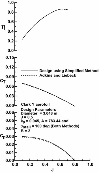
Comparison with a blade profile designed using the current method (denoted as ‘Simplified Method’), and the method of Adkins and Liebeck(Reference Adkins and Liebeck17) is shown in Fig. 12, while performance estimates are presented in Fig. 13. As the Adkins and Liebeck(Reference Adkins and Liebeck17) implementation did not have the current stall model implemented, the stall model was not used in the calculations. As seen, the computed geometries are close, with the present method showing a slightly greater chord inboard and smaller chord outboard than the Adkins and Liebeck(Reference Adkins and Liebeck17) formulation. The estimated pitch distributions are essentially identical. The two blade profiles were then analysed, yielding Fig. 13. For the thrust and power coefficient, the present method shows slightly higher loading, following from the chord discrepancy. The calculated η for the two blade designs is very close. Considering the simplicity of the design procedure, the close accord shown with the Adkins and Liebeck method is encouraging.
Propeller blade design comparison.

Analysis of designed propellers.

3.0 CONCLUSIONS
A non-iterative analysis procedure is presented for estimating the performance of propellers based on simplified vortex theory. Aerofoil data look-up tables are replaced with an analytic model, which in turn is coupled to a stall model. The approach is clearly elucidated as is the determination of the required inputs. Numerous comparisons of the method with experimental data are presented for validation, ranging from a full-scale propeller to those used for radio-controlled aircraft. The stall model is shown to provide effective representation of the thrust and power coefficients at low advance ratios. The method is also extended to serve as a design tool where optimal blades may be designed for a prescribed thrust or power.
ACKNOWLEDGEMENTS
The author would like to thank the reviewers for their comments and suggestions.