1. INTRODUCTION
Recently, the concept of using quantum physical devices to perform computation has received much attention caused by the celebrated factoring algorithm proposed by Shor (Reference Shor1994). This algorithm provides an exponential speed-up in comparison to all known classical factoring algorithms. Unfortunately, increased efforts following this promising result did not return any further developments as impressive. More recent results have cooled expectations that proved to be too optimistic (Bennett et al., Reference Bennett, Bernstein, Brassard and Vazirani1997; Bernstein & Vazirani, Reference Bernstein and Vazirani1997; Beals et al., Reference Beals, Buhrman, Cleve, Mosca and de Wolf2001), and it still remains unclear whether quantum computers (QCs) will provide an alternative superior to classical computation.
Yet the concept of computational power provides a fundamentally new language for studying the relationship between classical and quantum physics. Therefore, even modest speed-ups of quantum algorithms (QAs) compared to classical algorithms might provide further insight into the fundamental differences between classical and quantum physics. This can be helpful in estimating the computational benefit of QCs.
Unfortunately, the design and development of QAs is a very cumbersome task, mainly because of the nonintuitive character of quantum physics. Thus, it is reasonable to investigate automated algorithm design techniques in the development of new QAs. The usage of genetic programming (GP) was pioneered by Williams and Gray (Reference Williams and Gray1998), who used this approach to decompose a given quantum transformation into a sequence of elementary quantum gates. Another approach, used by Spector et al. (Reference Spector, Barnum, Bernstein, Swamy, Spector, Langdon, O'Reilly and Angeline1999), enabled the development of quantum circuits without knowing the quantum transformation in advance. Since then, several related strategies using GP to aid the development of QAs have been proposed and investigated by several authors (e.g., Leier & Banzhaf, Reference Leier and Banzhaf2003a, Reference Leier and Banzhaf2003b; Massey et al., Reference Massey, Clark and Stepney2004).
Here we present our GP system that we used to develop two formerly unknown better-than-classical QAs. We start with an introduction to quantum computation by means of the blackbox model of computation in Section 2. In Section 3 we present our GP system and discuss the conditions a fitness function should fulfill to facilitate the development of QAs. The QAs that we developed are presented in Section 4. Section 5 concludes.
2. QUANTUM COMPUTATION AND THE BLACKBOX MODEL OF COMPUTATION
An informative introduction to the complex topic of quantum computation can be found in Rieffel and Polak (Reference Rieffel and Polak2000). For a comprehensive overview we defer the reader to the book of Nielsen and Chuang (Reference Nielsen and Chuang2000).
A large class of QAs can be formulated using the blackbox model of computation (Beals et al., 2001). In this contribution we restrict our investigations to blackbox problems only.
2.1. Blackbox model of computation
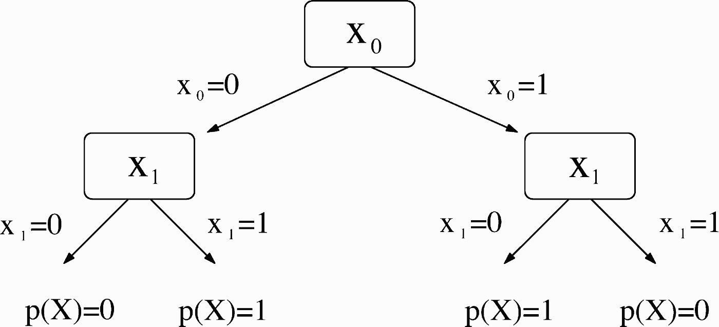
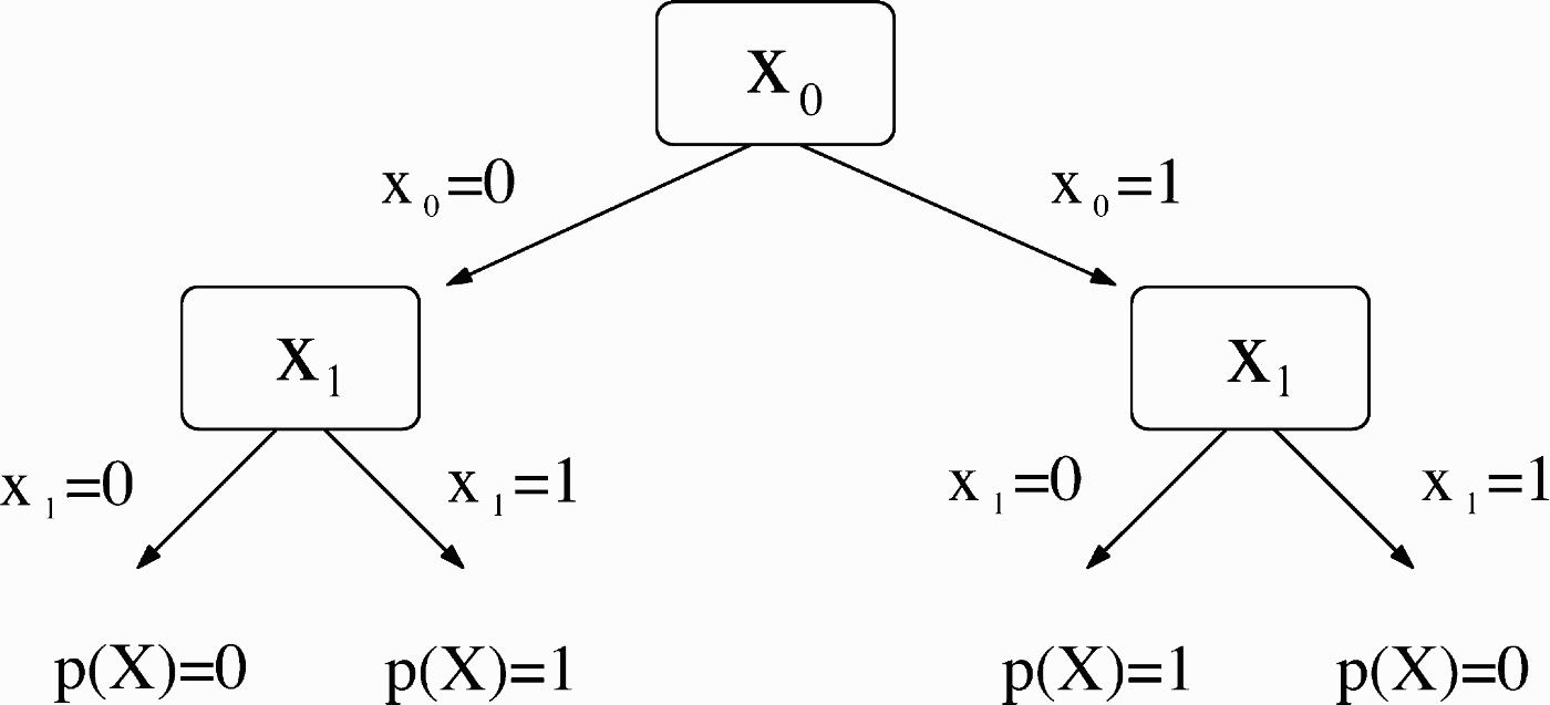
A blackbox X = (x 0, x 1, … , x N−1), also referred to as an oracle, consists of N Boolean variables x i with x i ∈ {0, 1}. On input i, the oracle returns the Boolean variable x i. Usually one wants to compute a Boolean property p(X) of such a blackbox using as few oracle queries as possible. The number of these queries is also called query complexity, which is the relevant complexity measure in this context.Footnote 1 A classical algorithm that computes property p(X) of a blackbox X can be represented by a decision tree with the kth query depending on the outcome of the k − 1 previous queries (see Fig. 1).
A classical decision tree that computes the parity p(X) of the blackbox.
Consider, for example, the parity problem: one wants to know if a binary string x N−1x N−2⋯x 0 of length N contains an even or an odd number of entries x i with x i = 1.
As can be seen in Figure 1, a classical decision tree that computes the parity of the blackbox X = (x 0, x 1) has to query the two elements one after the other.
Before we introduce the notation and essential ideas of quantum computing, we want to stress the main resource used by QCs to reduce the number of oracle queries: it is the exploitation of superpositions and interference of states that enables QCs to query several blackbox elements simultaneously.
From now on we distinguish between single-issue QCs and ensemble QCs. A single-issue QC denotes a single quantum system like the ions of an ion trap that is used for computation. An ensemble QC denotes a large number of quantum systems that are used for computation. The NMR sample of a liquid state NMR-QC, for example, contains ~1018 molecules, each a valid QC.
2.2. Single-issue QCs
A bit is defined to be either in the state 0 or in the state 1, whereas a quantum bit (qubit) can be in a superposition of both states. In quantum physics a physical state j (here j ∈ {0, 1}) is represented by a vector denoted by |j〉. With this notation the superposition |ψ〉 over both states represents a qubit and looks as follows:

The probability amplitudes α, β are used to calculate the probabilities |α|2, |β|2 that a measurement returns the state |0〉, |1〉, respectively. The probability to measure either state |0〉 or state |1〉 has to be |α|2 + |β|2 = 1.
A quantum system composed of several qubits is called a quantum register. The notation |i 1i 0〉 ≡ |i 1〉|i 0〉 ≡ |i 1〉 ⊗ |i 0〉 with i 0, i 1 ∈ {0, 1} describes a two-qubit register; ⊗ denotes the tensor product. This notation can easily be extended to describe n-qubit registers. A state like  that is not decomposable into a tensor product of the subsystems' states is called entangled:

where α1, α0, β1, β0 ∈ ℂ. Entanglement is a resource necessary to query blackbox elements in parallel using superpositions and binary encoding (see Lloyd, Reference Lloyd2000). The states |00〉, |01〉, |10〉 and |11〉 define the computational basis for the vector space of two-qubit states. With (1, 0, 0, 0)t ≡ |00〉, (0, 1, 0, 0)t ≡ |01〉, and so forth, the state |ψ〉 above is represented by the vector  .
It is well known that any arbitrary quantum operation (unitary transformation) can be decomposed into a sequence of unitary quantum operations on one and two qubits (Nielsen & Chuang, Reference Nielsen and Chuang2000). This is somehow similar to the fact that any Boolean function can be decomposed into a sequence of elementary logic gates (e.g., NOT, AND, OR). Because quantum gates are described by continuous parameters it is, however, only possible to approximate such an operation by a sequence of elementary one- and two-qubit gates, taken from a discrete set, up to an error ɛ (Nielsen & Chuang, Reference Nielsen and Chuang2000). The elementary one-qubit gates we used in our investigation are the Hadamard gate H and a discrete set of the rotation gates Rx(αk) and Ry(αk). The discrete value αk is calculated by αk = −π + k · 2π/ξ with k ∈ {1, … , ξ}, where ξ ∈ ℕ is chosen dependent on the desired accuracy of the approximation. With the Pauli matrices σx, σy, σz and the identity matrix 𝕀 defined by
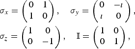
the one-qubit gates Rx(αk) and Ry(αk) are given by

The Hadamard gate is defined by
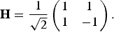
Hadamard gates are used by us only for convenience since the one-qubit gates Rx(αk), and Ry(αk) would be already sufficient to create any arbitrary one-qubit gate U via (see Nielsen & Chuang, Reference Nielsen and Chuang2000):

A single discrete two-qubit operation called CNOT-gate, together with the discrete set of one-qubit gates defined above is sufficient to provide a complete set of unitary operations that is capable of approximating any arbitrary unitary operation up to the desired accuracy (Nielsen & Chuang, Reference Nielsen and Chuang2000). The CNOT-gate is defined by its action on a two-qubit state:

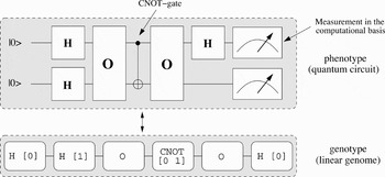
Here, ⊕ denotes the XOR operation between the Boolean variables l and m. Analogous to a Boolean circuit it is possible to define a quantum circuit as a directed acyclic graph whose nodes are labeled by elementary quantum gates like the ones defined above. Because of reversibility of quantum operations and the no-cloning theorem (Nielsen & Chuang, Reference Nielsen and Chuang2000) any elementary quantum gate has as many inputs as outputs. An example of such a quantum circuit on two qubits together with the final measurements can be found in the upper part of Figure 2.
A quantum circuit is represented by a linear list (linear genome) of the quantum gates used. The sequence of quantum gates is obtained by reading this linear list from left to right. H [Reference Beals, Buhrman, Cleve, Mosca and de Wolf1] denotes a Hadamard gate H that is applied to qubit 1. CNOT [0 1] denotes a CNOT gate where qubit 0 is the control qubit and qubit 1 is the target qubit.

2.3. Ensemble QCs
Up to now, we only considered single quantum systems whose state is known. In this case, one usually speaks of a pure state of the quantum system. Even in single-issue QCs, unavoidable decoherence processes turn the initially pure states into mixed states. Such states cannot be described by a single quantum state. The appropriate formalism for their description is the density operator that describes systems where one only knows the probability p i that a certain pure quantum state |ψi〉 occurs.
Before we can define this operator we have to introduce the dual state 〈ψ| of a quantum state |ψ〉. Using this notation the scalar product of two quantum states |ψ〉 and |φ〉 is given by 〈ψ|φ〉. With |ψ〉 = α|0〉 + β|1〉 ≡ (α, β)t one gets 〈ψ| ≡ α*〈0| + β*〈1| ≡ (*α*, β*). Using this notation the normalization condition can be formulated as 〈ψ|ψ〉 = αα* + ββ* = 1. Another necessary concept used in quantum physics is the concept of the measurement operator, which usually can be represented by a Hermitian matrix. The expectation value 〈M〉 of a measurement described by the measurement operator M for a quantum system in the pure state |ψ〉 is calculated by

Here ρ denotes the density operator of the pure quantum state |ψ〉. With |i〉 denoting a basis state of the vector space of our quantum system, the trace tr{A} of an operator is defined by tr{A} = ∑i〈i|A|i〉 with i ∈ {0, 1, … , 2n − 1} where n denotes the number of qubits. A measurement can be described by a projection operator P. Consider, for example, the state |ψ〉 = α|00〉 + β|01〉 + γ|11〉. If one wants to know the probability to measure the leftmost qubit to be in state |0〉 the corresponding measurement operator looks as follows:

Calculation of 〈P0〉 returns 〈P0〉 = |α|2 + |β|2. This procedure provides the formal framework to calculate measurement probabilities for pure states. Nevertheless, as we only consider measurements in the computational basis we added the absolute squares of the probability amplitudes directly, as it is obvious which probability amplitudes are involved without using this time-consuming calculation scheme.
A mixed state that is in the state |ψi〉 with probability p i is represented by ρ = ∑ip i|ψi〉〈ψi|. The expectation value 〈M〉 for a mixed state is calculated by

Let the unitary operator A describe a quantum computation and let ρinit describe the initial state of the quantum register. The final quantum state ρfin can be calculated by ρfin = AρinitA+, where A+ is the transposed and complex conjugate of the matrix A: (A+)ij = (A−1)ij = A*ji. In our investigations concerning ensemble QCs we only considered liquid-state NMR-QCs (an introduction to NMR-QCs can be found in Nielsen & Chuang, Reference Nielsen and Chuang2000). Here, the initial state is the thermal state

where we have set  and invoked the high-temperature approximation. Here, ℋ denotes the Hamiltonian of the spin system, ωi is the Larmor frequency of the ith spin (qubit), and Iz(i) the corresponding spin operator:
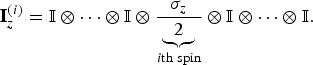
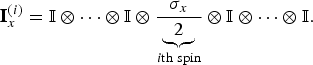
In liquid-state NMR quantum computation one measures the magnetization of the ith nuclear spin in the molecules of the NMR sample along the x and y axis. We restricted ourselves to measurements along the x axis, which are described by measurement operators of the form
3. EVOLVING BLACKBOX QAs USING GP
In this section we take a closer look at the GP system in the development of QAs that will be presented in Section 4. Our GP system was used to evolve quantum circuits for small problem instances on a few qubits only. These circuits were examined for scalability to find the corresponding uniform circuit family and thus the algorithm that solves the problem. At first we describe how a quantum circuit is represented by our GP system. Then we present the different oracle gates used. Because we evolved quantum circuits for single issue QCs as well as for ensemble QCs the section about fitness functions is divided into two parts.
3.1. Representation of quantum decision trees in our GP system
As already mentioned in the last section, a computation of a blackbox's property can be visualized by a decision tree. According to Buhrman and de Wolf (Reference Burhman and de Wolf2002) a quantum decision tree is defined by a sequence of oracle gates O that represent blackbox calls, alternating with unitary transformations Ui:

Such a sequence can also be used to simulate classical decision trees (see Buhrman & de Wolf, 2002). Consider a single-issue QC; here, the sequence denoted by the unitary transformation A is applied to the initial state |ψinit〉 = |0 · · · 0〉. Measuring the readout-qubit of the final state |ψfinal〉 = A|ψinit〉 returns a binary value. If this binary value equals p(X) for all blackboxes one says that the quantum decision tree computes the property p(X) of the blackbox encoded by the oracle gate O.
It is adequate to represent quantum decision trees by quantum circuits. To do that one needs a complete set of one-qubit and two-qubit gates. In addition, one needs the set of oracle gates O representing the blackboxes X. In principle, the measurement of a readout qubit should be sufficient to decide the property p(X) of a blackbox X; nevertheless, algorithms like the Deutsch–Jozsa (DJ) algorithm answer the problem by measuring several qubits (Deutsch & Jozsa, Reference Deutsch and Jozsa1992). This procedure makes it possible to dispense with the additional output qubit and additional quantum operations necessary to encode the answer into this output qubit. Now that the answer to the posed problem cannot be obtained any more by measuring the state of a single qubit (output qubit), the QA has to return different measurement results for those blackboxes X that differ in their property p(X). How this can be realized is shown in Section 3.3.1. We decided to perform all measurements possible on the final state |ψfinal〉 to check if one of these measurements returns different results for blackboxes X that differ in their property p(X).Footnote 2 If the state |ψinit〉 is encoded by n qubits we thus perform all n one-qubit measurements, all n(n −1)/2 two-qubit measurements and so on.Footnote 3
As in the work of Spector et al. (Reference Spector, Barnum, Bernstein, Swamy, Spector, Langdon, O'Reilly and Angeline1999), we have chosen a linear genome to represent quantum circuits in our GP system (see Fig. 2). Because a quantum gate is specified by several parameters like rotation angles, control-qubits, and so forth, one has to decide where these additional data are to be stored and how they are to be manipulated by the evolutionary process. The most natural method is to consider a quantum gate and these additional parameters as a unit, allowing the evolutionary process to only modify the unit as a whole. Because any QA starts with the initial state |ψinit〉 and qubits to be measured are specified by a global variable, we did not encode these parameters into the genome. As stated in the caption of Figure 2, the sequence of quantum gates is obtained by reading the genome from left to right.
3.2. Oracle gates
To see if a quantum circuit correctly calculates the property p(X) of blackbox X one has to check this circuit for all blackboxes. The blackboxes are encoded into a quantum system via the oracle gates O, so these gates provide the fitness cases the quantum circuit is to be tested with. Depending on the property a quantum circuit has to compute, the number of blackboxes (oracles) that are to be tested can grow superexponentially. Thus, not only the effort to simulate a quantum system grows exponentially with the number of qubits, but also the number of oracles that are to be tested increases quickly rendering an investigation of quantum circuits with many qubits impractical. One should, therefore, strive to reduce the number of oracles to be tested.
One possibility to do that is to use an encoding of the blackbox values into a quantum state that enables a reduction in the number of oracles to be tested. The DJ problem for a single query qubit can be used to illustrate this procedure.Footnote 4 Here, the constant blackboxes X 1 = (0, 0), X 2 = (1, 1) with p(X 1,2) = 0 are to be distinguished from the balanced blackboxes X 3 = (0, 1), X 4 = (1, 0) with p(X 3,4) = 1. If one employs the usual definition of the oracle gate

one has to test each of the four different oracles. Because the DJ problem can also be solved by using the following oracle gate (Collins et al., Reference Collins, Kim and Holton1998):

it is possible to find a quantum circuit that solves this problem by testing two oracles only. Using the latter definition returns the same oracle, up to a global phase shift, for the two constant blackboxes: O1,2 = ±𝕀. For the two balanced blackboxes one gets: O3, 4 = ±σz. Because global phase shifts are not measurable, it is not necessary to test all four different oracles but only the oracle O1 = I and O3 = σz. A further advantage of this method is that one needs no additional output register as would be the case with the definition in Eq. (4).
Nevertheless, it depends on the property p(X) one is interested in, whether an encoding of the blackbox entry x k into the phase (−1)x k is possible. If, for instance, one wants to calculate the property p(X 1) = 0 and p(X 2) = 1 with X 1 = (0, 0) and X 2 = (1, 1) it is impossible to encode the blackbox entries into phase shifts, because then both cases become indistinguishable for a quantum system as they only differ by a global phase shift. To see if an encoding into a local phase shift via Eq. (5) is possible one thus has to check if for every pair of blackboxes X = (x 0, x 1, … , x n) and  the condition
 holds. Here,
 denotes the negation of the binary variable x k.
Up to now we only considered blackboxes X whose entries were binary values. In Simon's problem (Simon, Reference Simon1994) one investigates blackboxes X = (x 0, x 1, … , x N−1) with x k ∈ {0, 1, … , l − 1} and l ∈ ℕ. If one applies the approach of Eq. (4), one needs an output register size of log2(l) qubits. Up to now, both, in simulation and in experiments, only a few qubits are realizable, and thus this approach is not reasonable for l ≫ 1. Therefore, we used a combined approach where the blackbox entries with  are encoded partially into a phase shift and partially into an m-qubit output register. We write the decomposition x k(phase) of
 for blackbox entry x k if it is decomposed into part x k(phase) encoded into a phase shift, and part
 encoded into an output register. Consider, for example, blackbox entries x k ∈ {0, … ,15}. With two output qubits one only can encode four different values. Therefore, one needs another four different phase shifts to encode unambiguously. The value x k = 13 would thus be decomposed into x k(phase) = 3 and
 = 01. This decomposition follows from the binary representation of 13: 1101. The two rightmost values are the assignment for
 , the integer represented by the two leftmost qubits is the value of the phase shift.
In general, the oracle gate looks like:

with k ∈ {0, 1, … , N − 1} and b, x k ∈ {0, 1}m. Here, we write b ⊕  to denote the bitwise XOR-operation between the m-bit value b and the m-bit value
 . We write k to denote the binary decomposition of the integer k. For m = 0, the blackbox entries are entirely encoded into phase shifts, which saves log2(l) qubits. Nevertheless, as before, not every blackbox problem can be encoded using this approach. For m = log2(l) the blackbox entries are completely encoded into the output register.
In Section 4 we will present a QA that was evolved using oracle gates as defined in Eq. (6).
3.3. Fitness functions
The definition of the fitness function is the most sensitive part in setting up the GP system because here one has to make assumptions that might turn out to be ill-suited for evolving quantum circuits. The mathematical structure of quantum physics allows to define a metric on the space of unitary operators, that is, quantum circuits, enabling the assignment of a step length to mutation and crossover operators. Small mutations, according to this measure, lead to small changes in the measured expectation values (see Nielsen & Chuang, Reference Nielsen and Chuang2000). Because the fitness function has to depend on these expectation values it is desirable that it retains this property. We would like to emphasize, however, that all QAs presented here were evolved using a fitness function that did not fully obey this condition.
3.3.1. Fitness function for single issue QCs
We will motivate the definition of the fitness function by means of the DJ problem for blackboxes with four elements. Nevertheless, the problems we evolved QAs for that are presented in this article are the parity problem and a special case of the hidden subgroup problem and not the DJ problem. Both problems were treated by our GP system using fitness functions similar to the one we now discuss.
For four blackbox elements the DJ problem is to distinguish between the constant blackboxes X 1 = (0, 0, 0, 0),  with p(X 1,2) = 0 and the balanced blackboxes:

with p(X i≥3) = 1. According to Section 3.2 this problem can be solved by encoding the blackbox entries into phase shifts via the oracle gates defined by Eq. (5). Thus fitness depends on the measurement results for the four blackboxes X 1 = (0, 0, 0, 0), X 3 = (0, 0, 1, 1), X 4 = (0, 1, 0, 1) and X 5 = (0, 1, 1, 0). The oracle gates of the remaining blackboxes differ from the oracle gates O1, O3, O4, and O5, which represent the four blackboxes mentioned above by a global phase shift only (see also Section 3.2).
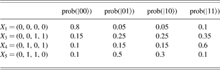
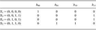
Table 1 shows measurement probabilities for a fictive quantum circuit applied to input state |ψinit〉 = |00〉. How well does this circuit decide between constant and balanced blackboxes? We consider a quantum state |i 1i 0〉 to be measurable with a sufficient probability if prob(|i 1i 0〉) > 1/N, where N is the number of quantum states we want to distinguish (here, N = 4) and prob(|i 1i 0〉) is the probability to measure state |i 1i 0〉. A binary variable b i 1i 0 indicates whether quantum state |i 1i 0〉 fulfills this condition (see Table 2).
Measurement probabilities for a fictive quantum circuit
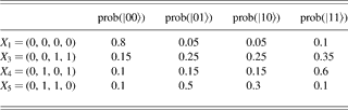
prob(|i 1i 0〉), the probability of measuring quantum state |i 1i 0〉 after applying the quantum circuit to |00〉.
Results obtained from Table 1 by setting the binary value bi1i0 = 1 if p(|i1i0〉) > 1/4
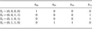
Using b i 1i 0 for each blackbox X, one has to check whether b i 1i 0 = 1 for constant and balanced blackboxes simultaneously. In this case, the quantum circuit is not able to distinguish between the different blackboxes. If, on the other hand, there is a difference in the outcome, we consider the circuit a promising candidate for solving the problem and the error probability of this circuit is calculated to check how well the circuit distinguishes between the two kinds of blackboxes.
According to Table 2, only the constant blackbox X 1 is mapped to state |ψfinal〉 = |00〉. The quantum circuit is therefore able to distinguish between constant and balanced blackboxes. However, as indicated in Table 1, there is a certain probability that a blackbox, for instance X 3 = (0, 0, 1, 1), could be classified as constant (with a probability of 15%). Inspection of Table 1 shows further that the probability of misclassifying the balanced blackboxes X 4 = (0, 1, 0, 1) and X 5 = (0, 1, 1, 0) is 10% in both cases. It can also be calculated that the error for a constant blackbox is 20%.
It is better, therefore, to have the fitness function depend on at least two parameters. The first parameter is called clash, and quantifies how often it is not possible to distinguish between constant and balanced blackboxes. Another parameter,
, denotes the highest probability of a misclassification. In the example we have
= 0.2, the error probability that a constant blackbox is classified to be balanced. As further parameters we used
denoting the average error,
to denote the number of oracle gates, and
to denote the total number of quantum gates used by the quantum circuit.
Similar to the approach used by Spector et al. (Reference Spector, Barnum, Bernstein, Swamy, Spector, Langdon, O'Reilly and Angeline1999), these parameters were used to create a lexicographic fitness function represented by a vector of the form

The position of the parameters in this vector represents their priority, decreasing from left to right.
This fitness function is to be contrasted with that of Spector et al. (Reference Spector, Barnum, Bernstein, Swamy, Spector, Langdon, O'Reilly and Angeline1999), who measure the probability of the state of a single qubit. The advantage of our approach is that an evolved quantum circuit that solves the DJ problem has the possibility to resemble the original one, which decides the property of a blackbox with 2n elements by n measurements. Therefore, we do not need additional quantum gates necessary to solve the problem by the measurement of a single qubit, only. Such additional quantum gates would make it difficult to extract the functionality and thus the scalability of a quantum circuit.
3.3.2. Fitness function for ensemble QCs
A liquid-state NMR-QC realizes qubits by the spin states of the molecule's spin-1/2 nuclei. Because a liquid-state NMR-QC performs its computations on an ensemble of molecules, the fitness function has to be derived from expectation values 〈Ix(i)〉 of the measurement operator Ix(i) as described in Section 2.3.
Consider, for example, a two-qubit system. Here, the initial state is described by

In contrast to Eq. (2), we skipped the term proportional to the identity matrix as it does not contribute to the expectation values 〈Ix(i)〉.
A quantum circuit described by the unitary transformation A maps this state to ρ = AρthA+. The measurement of the ith spin's magnetization along the x axis is calculated by

Analogous to the single-issue QC, all combinations of measuring the spins' magnetization are performed to check if one of these returns different results for blackboxes X that differ in their property p(X). In our example, one therefore has to calculate 〈M〉 for M = Ix(0), M = Ix(1), and M = Ix(0) + Ix(1).
To quantify how well a promising circuit solves the problem, we divided the interval [−|〈M〉|, … , |〈M〉|] of possible measurement results in several disjoint subintervals.Footnote 5 If the measurement results for blackboxes with p(X) = 0 belong to different subintervals than the measurement results for blackboxes with p(X) = 1 we consider the circuit a promising candidate for solving the problem. To decide how well this circuit can distinguish between both types of blackboxes we calculate the minimal distance between the corresponding measurement results. The variable
denotes this minimal distance, whereas the variable
denotes the average distance.
The fitness function is represented by the vector

Analogous to the fitness function introduced in the last section we used a lexicographic ordering of the vector components with
, the most significant one. Once again, an optimal circuit would have minimal values in all components of its fitness function.Footnote 6 Nevertheless, we still have the problem that the component
does not respect the continuity of the expectation values in the step length of mutation operators. When
= 0, the parameters
and
become significant, and these parameters respect the continuity of the expectation values in the step length of mutation operators.
4. QAS DEVELOPED BY GP
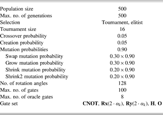
In this section we present two new better than classical QAs that were developed with the help of our GP system using the parameters shown in Table 3.
Parameters of the GP system that evolved the circuits in Section 4.1 and 4.2.
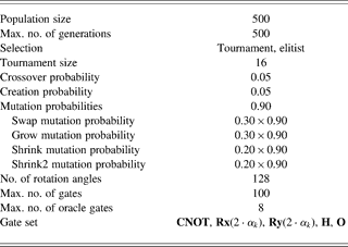
Shrink2 mutation denotes a mutation operator that concatenates quantum gates. The rotation angle is specified by the integer k ∈ {0, 1, … , 127} via αk = −π + (k + 1) · 2π/128.
Both algorithms were found by applying the GP system to the smallest instances of the corresponding problem. The circuits returned by the GP system were examined for scalability to find the corresponding uniform circuit family and thus the algorithm.
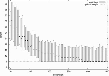
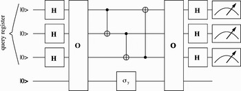
Figure 3 shows the length distribution of the best individual found in each generation for 60 independent runs of the GP system for the n = 3 qubit parity problem. This result indicates that 50% of the runs find the optimal quantum circuit after approximately 375 generations. The genome of an optimal solution is
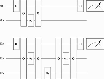
This graph shows the length distribution (first, second, and third quartiles) of the best individual in each generation for 60 independent runs of the GP system for the n = 3 qubit parity problem. The optimal algorithm is presented in the lower part of Fig. 4. A horizontal bar denotes the median (second quartile). The lower, upper end of each box indicates the first, third quartile, respectively.


A run (500 generations) takes about 27 min on a single core of an AMD Opteron 870 processor. Here,
denotes that the one-qubit gate Ry(2 · α95) is applied to qubit 1, where α95 = π/2. The quantum circuit in the lower part of Figure 4 can be derived from this one by replacing
with
and
with
. Nevertheless, the functionality of the circuit is not altered by these replacements; hence, the above genome represents an optimal solution.
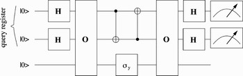
These two exact parity circuits for n = 2 qubits (top) and n = 3 (bottom) qubits found by the GP system were sufficient to extract the general scaling mechanism for an arbitrary number of qubits (see Stadelhofer et al., Reference Stadelhofer, Suter and Banzhaf2005).

The optimal quantum circuit for the n = 2 qubit parity problem is found with almost certainty after 500 generations (running time = −1 min). One in three runs of the GP system returned the optimal quantum circuit for the special case of the hidden subgroup problem (n = 3 qubits) when the population contains 2500 individuals (running time = ~7 min). For n = 4 qubits, the optimal quantum circuit was found in 3 of 100 runs (running time = ~9 h).
4.1. A quantum algorithm that solves the parity problem
When the parity problem is formulated as a blackbox problem, the desired property of parity can be written as the Boolean function:

Here, ⊕ denotes the XOR operation (addition Modulo 2). A classical computer has to call the oracle with each of the N possible inputs i to determine p(X), whereas Beals et al. (2001) and Farhi et al. (Reference Farhi, Goldstone, Gutmann and Sipser1998) showed that a QC requires only N/2 oracle calls.
We found an optimal QA in the sense of Beals et al. (2001) and Farhi et al. (Reference Farhi, Goldstone, Gutmann and Sipser1998). This algorithm can be applied to pure and mixed states. Variants also found by the GP system could be optimized for application to ensemble QCs like liquid-state NMR-QCs such that the number of oracle calls decreases exponentially relative to a single-issue QC provided the signal/noise ratio is sufficiently high (Stadelhofer et al., Reference Stadelhofer, Suter and Banzhaf2005). The gates used by the QA are Hadamard gate H, NOT gate σx = ıRx(π) and oracle gate O. Queried by the basis state |i〉 the oracle O defined in Eq. (5) returns the binary value x i ∈ X encoded into a phase shift of the querying state.
By means of the circuit that solves the parity problem for n = 2 query qubits in the upper part of Figure 4 we demonstrate the functionality of our parity algorithm. With two query qubits four different blackbox elements can be addressed; therefore, one only has to check the circuit for the 16 different blackboxes X = (x 0, x 1, x 2, x 3) with x i ∈ {0, 1}. Because we use oracle gates that encode blackbox elements into phase shifts it is sufficient to check the circuit for eight different blackboxes (see also Section 3.2).
The computation starts with the initial state |ψinit〉 = |00〉 that is transformed into the superposition  by the first Hadamard gate H. Thus, the oracle call queries two blackbox elements in parallel. To query the remaining two elements a NOT operation is applied to the remaining qubit, then the oracle is called again. After a final Hadamard operation the final state is given by
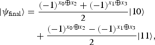
which is equivalent to

Thus, one finds the rightmost qubit to be in state |0〉 if p(X) = 0, and one measures this qubit in state |1〉 if p(X) = 1. It follows that the parity of the four elements of the blackbox can be computed by only two oracle calls because, due to the superposition over two states, each single call returns two blackbox elements.
As shown in Stadelhofer et al. (Reference Stadelhofer, Suter and Banzhaf2005), this circuit can be scaled up to an arbitrary number of qubits.
With our algorithm, parity is obtained by a single one-qubit measurement compared to the 2n−1 measurements necessary by the parity algorithm proposed by Beals et al. (2001) or to the n measurements used by the parity algorithm in Farhi et al. (Reference Farhi, Goldstone, Gutmann and Sipser1998). The latter parity algorithm is somewhat similar to ours though. Instead of a single NOT operation between every two oracle calls an n-qubit gate is used, which itself has to be decomposed into elementary quantum gates. Therefore, our algorithm is more efficient with respect to the number of necessary gate operations other than oracle calls.
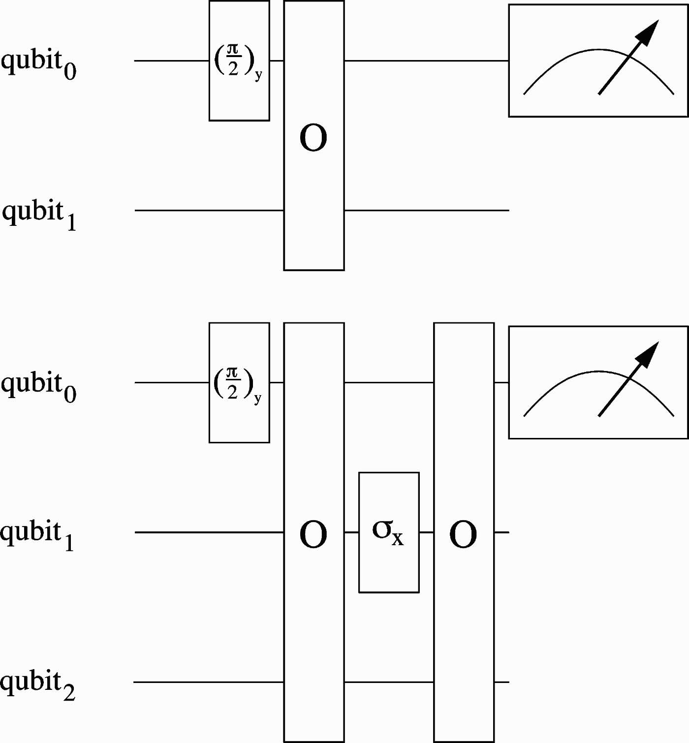
We also used our GP system to search QAs for ensemble QCs (liquid-state NMR-QCs) and, indeed, were able to find the quantum circuits presented in Figure 5 that need fewer oracle calls than the circuits for single issue QCs presented above.
Mixed-state parity circuits found by the GP system for n = 2 (top) and n = 3 (bottom) qubits. The (π/2)y-gate corresponds to the rotation Ry(π/2). The measurement-gate symbolizes a measurement of the magnetization along the x axis. In both cases one measures 〈Ix(0)〉 = 0 if p(X) = 1 and 〈Ix(0)〉 = ±ω0/4 if p(X) = 0.
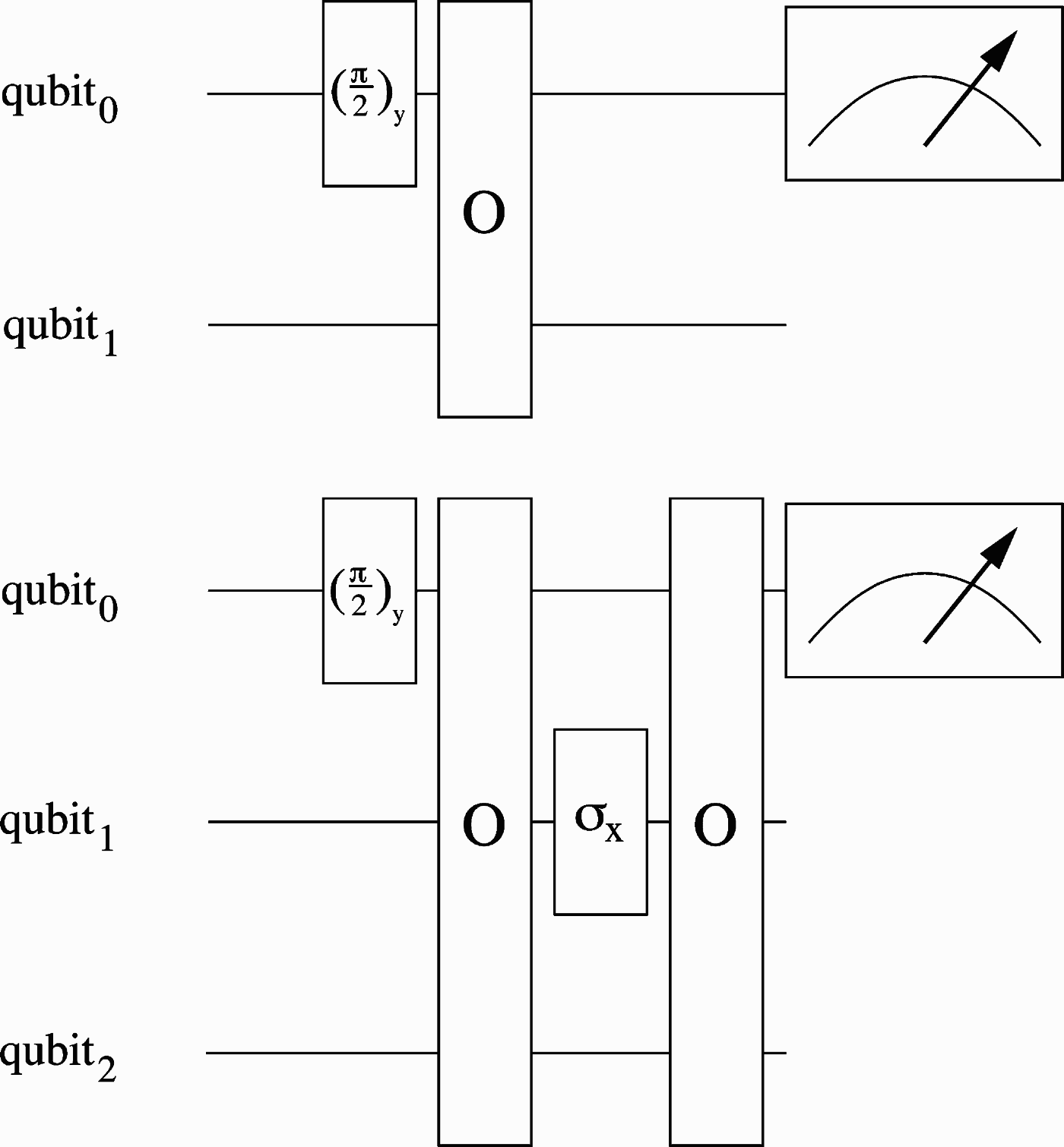
These ensemble quantum circuits appear to violate the lower bounds proven in (Farhi et al., Reference Farhi, Goldstone, Gutmann and Sipser1998; Beals et al., 2001). However, as illustrated in Appendix A, these proofs seem not to apply to ensemble QCs.
4.2. A quantum algorithm that solves a special case of the hidden subgroup problem
The first instance of the problem we consider in this section is to distinguish between blackboxes X ∈ A with A = {(a, a, a, a)} and blackboxes X ∈ B with

where a ≠ b and a, b ∈ {0, 1, 2, 3}. To solve this problem we first tried to encode the blackbox entries entirely into phase shifts via the oracle gate  . This approach did not return satisfactory results. Therefore, we tried the combined approach defined in Eq. (6). As a blackbox call can return four different values x k ∈ {0, 1, 2, 3} for k ∈ {0, 1, 2, 3} there is only the following possibility to use a combined encoding into a phase shift and an output register:

with b, x k(phase), x k(XOR) ∈ {0, 1} and k ∈ {0, 1, 2, 3}. Here, the blackbox entries are decomposed into the two binary values x k(phase) and x k(XOR). Consider, for example, the blackbox X = (0, 3, 0, 3): decomposing the blackbox entries into two binary values returns the alternative representation X′ = (00, 11, 00, 11). One gets

The oracle gate O(0,3,0,3), therefore, looks like
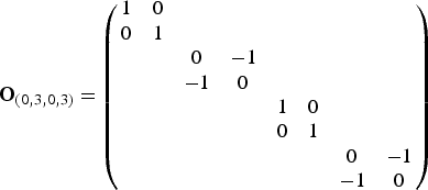
The weakness of this approach is that it requires an additional output qubit. Nevertheless, this still is an advantage over the two additional qubits necessary for a traditional encoding of the blackbox entries x k ∈ {0, 1, 2, 3} into an output register. In addition, it is still possible to reduce the number of blackboxes that are to be tested: if one uses the oracle defined in Eq. (12), the blackbox X 1 = (0, 0, 1, 1) and the blackbox X 31 = (2, 2, 3, 3) have the same oracle gate up to a global phase shift. Therefore, it is sufficient to only test X 1. It follows that one only has to test two instead of the four blackboxes X ∈ A and 18 instead of the 36 blackboxes X ∈ B. Thus, the evaluation of a quantum circuit by the GP system is reduced by a factor of 2 × 2 in comparison to the traditional encoding. The quantum circuit returned by the GP system is shown in Figure 6.
This circuit distinguishes between blackboxes X ∈ A and blackboxes X ∈ B by mapping the initial state |ψinit〉 = |00〉 of the query register to the final state |ψfin〉 = |00〉 if X ∈ A, otherwise, the state |00〉 of the query register has a probability amplitude of zero. The gate σy is realized by Ry(π): σy = Ry(π).

To see if this quantum circuit can be scaled up to an arbitrary number of qubits we tried to find a related problem for blackboxes with eight elements (three query qubits). After several attempts we found a problem for which the GP system returned the quantum circuit shown in Figure 7. The problem solved by this circuit is to distinguish between blackboxes X ∈ A with A = (a, a, a, a, a, a, a, a) and blackboxes X ∈ B with

where a≠b and a, b ∈ {0, 1, 2, 3}.
This circuit distinguishes between blackboxes X ∈ A and blackboxes X ∈ B by mapping the state |ψinit〉 = |000〉 of the query register to the final state |ψfin〉 = |000〉 if X ∈ A, otherwise, the state |000〉 of the query register has a probability amplitude of zero.

The two instances of the problem presented above were sufficient to find the general structure of the problem that can be stated as the following special case of the hidden subgroup problem (i denotes the binary decomposition of the integer i).
One is given the finite Abelian group G = {0, 1}n of the size |G| = N = 2n and a subgroup H G. The group multiplication operation is the bitwise XOR operation (⊕). In addition, one is given a blackbox X = (x 0, x 1, … , x N−1) with x i ∈ {0, 1, 2, 3} and i ∈ G. One is promised that either X ∈ A or X∈ B, where X ∈ A denotes that only for H = G there exists an element g ∈ G such that xi = xj ⇔ i, j ∈ g ⊕ H, and X ∈ B denotes that only for H ⊆G with |H| = |G|/2 there exists an element g ∈ G with xi = xj ⇔ i, j ∈ g ⊕ H. Here, we used the notation g ⊕ H to denote the coset of H.Footnote 7 In addition to the usual definition of the hidden subgroup problem we required that x i ∈ {0, 1, 2, 3} and that the subgroups H to be distinguished contain N or N/2 elements, respectively. In the hidden subgroup problem (see Nielsen & Chuang, Reference Nielsen and Chuang2000) the group members need not be binary strings, and thus the group multiplication operation can be of a different type then the one used here. There, one is interested in the generating set of a subgroup H ∈ G, where |H| can be of any size. Knowing this generating set makes it possible to distinguish between subgroups H. Therefore, any algorithm solving the hidden subgroup problem solves the special case presented here as well.
Note that the problem this algorithm solves is not to distinguish between constant and balanced blackboxes, as in general not every balanced blackbox belongs to set B.
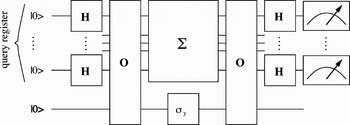
The general structure of quantum circuits that solve our special case of the hidden subgroup problem is shown in Figure 8.
Generalized circuit on (n + 1) qubits. The upper n qubits encode i ∈ {0, 1, … , 2n − 1}; Σ abbreviates the gate sequence CNOT0.1 − CNOT1.2 −⋯− CNOTn−2,n−1 − CNOTn−1,0. CNOTl,m denotes a CNOT gate where qubit l is the control qubit and qubit m the target qubit. This circuit distinguishes between blackboxes X ∈ A and blackboxes X ∈ B by mapping the initial n-qubit state |ψinit〉 = |0⋯0〉 of the query register to the final state |ψfin〉 = |0⋯0〉 if X ∈ A, otherwise, the state |0⋯0〉 of the n-qubit query register has a probability amplitude of zero.

This QA solves this problem exactly with two oracle calls only. An exact classical algorithm that solves this problem needs up to n + 1 blackbox calls (here: |G| = 2n), where n denotes the number of query qubits.Footnote 8 A probabilistic classical algorithm can solve this problem using k > 1 calls with an error probability of 2−k+1 (for |G| ≫ 1).
As shown in Brassard and Høyer (1998), Simon's QA can be generalized to a broader class of problems called Simon's hidden subgroup problems that are a subset of hidden subgroup problems. This generalized algorithm is probabilistic, and can also be used to solve the problem presented here. The error probability solving the problem decreases with 2−k+1 in the number k of repetitions of this algorithm. Because this generalized algorithm calls the oracle only once, k repetitions of the algorithm correspond to k oracle calls. In Brassard and Høyer (1998) the authors also present an exact algorithm capable of solving Simon's hidden subgroup problem, which in our case has to call the oracle three times.
It follows that the QA found with the help of the GP system is faster than any classical algorithm as well as the QAs known to us.
5. CONCLUSION
The successful development of two formerly unknown QAs presented in Section 4 demonstrates the usefulness of evolutionary methods for generating new QAs. Despite the fact that the fitness functions used did not fulfill the requirements we discussed in the beginning of Section 3.3 in every aspect, the results obtained are very promising.
We restricted our investigations to the blackbox model of computation where the Boolean property p(X) of a blackbox X is to be computed with a minimal number of blackbox calls. Our GP system only considers quantum decision trees that, after a sequence of oracles and quantum gates, reveal the property of the blackbox by a final measurement (see Section 3.1). This is similar to the approach used by Beals et al. (2001) in proving lower bounds for the parity problem. Surprisingly, the GP system returned quantum circuits that beat this lower bound on ensemble QCs. The error probability of these quantum circuits on a single issue QC is 1/2 (see Appendix A); nevertheless, running such a circuit several times on the same initial state makes it possible to solve the parity problem with an error probability that decreases exponentially in the number of repetitions.
Indeed, QAs like Simon's algorithm also use several independent runs of a QA to collect measurement results for a further classical treatment. At the current stage our GP system would not be able to evolve such hybrid algorithms for single-issue QCs. To our knowledge, such hybrid algorithms were not investigated by other authors (Spector et al., Reference Spector, Barnum, Bernstein, Swamy, Spector, Langdon, O'Reilly and Angeline1999; Leier & Banzhaf, 2003a; Spector, Reference Spector2004) who use GP to design QAs.
ACKNOWLEDGMENTS
The authors thank Dr. André Leier for helpful discussions. Financial assistance was provided by the Deutsche Forschungsgesellschaft through Graduiertenkolleg 726.
Ralf Stadelhofer studied physics from 1995 to 2001 at the University of Konstanz. From 2001 to 2004 he was a scholarship holder within the Materials and Concepts of Quantum Information Processing PhD program at the University of Dormund, Germany. Since then he has worked as the Chair of Bioinformatics at the University of Konstanz. Dr. Stadelhofer's interests focus mainly on inverse problems like the protein folding problem and the phase problem in X-ray crystallography.
Wolfgang Banzhaf was educated as a theoretical physicist and is now a Professor of computer science and Head of the Department of Computer Science at Memorial University of Newfoundland. In the last 20 years he has published more than 150 technical contributions, was lead author of a textbook on genetic programming, edited conference proceedings on topics of evolutionary computation and artificial life, and served as Editor in Chief of Genetic Programming and Evolvable Machines. His interests span a wide range of technical topics, from basic physics and computing to biology.
Dieter Suter works in experimental condensed matter physics in the Department of Physics at the Technical University of Dortmund. He obtained a PhD in physical chemistry from ETH Zürich in 1985, working on nuclear magnetic resonance (NMR). His postdoctoral work at Berkeley and ETH Zürich was in the fields of magnetic resonance and quantum optics. In 1995 he joined the faculty of the Technical University of Dortmund. In addition to quantum information processing, Dr. Suter is developing spectroscopic techniques in the fields of magnetic resonance and laser spectroscopy.
APPENDIX A: A PROBABILISTIC PARITY QUANTUM ALGORITHM
Usually (see, e.g., Farhi et al., Reference Farhi, Goldstone, Gutmann and Sipser1998; Beals et al., 2001) one only considers probabilistic algorithms that have an error probability of 1/2 − ɛ with 0 < ɛ ≤ 1/2 because their error probability can be reduced further by running them several times (Nielsen & Chuang, Reference Nielsen and Chuang2000). Here we exemplify how a quantum decision tree with an error rate of 1/2 can be used to solve the parity problem. To do so we investigate the behavior of a modified instance of the ensemble quantum circuit shown in the upper part of Figure A.1 on a single issue QC. For convenience, we added an additional qubit, a controlled gate and two Hadamard gates to this instance, which makes it possible to replace the measurement of the magnetization by a projective measurement in the computational basis, as usual for single issue QCs (see Fig. A.1). The original ensemble circuit returns 〈Ix(0)〉 = 0 for blockboxes X with p(X) = 1 and 〈Ix(0)〉 = ±ω0/4 if p(X) = 0. For the single-issue QC this corresponds to the additional qubit's final state |ψ〉 = |0〉 or |ψ〉 = |1〉 if p(X) = 0. If p(X) = 1, the additional qubit's final state is described by the superposition  . It follows that for p(X) = 1 a measurement will return the state |0〉 or |1〉 with equal probability, whereas for p(X) = 0, only one of these two states will be measured with a nonzero probability. Thus, a single run of the quantum circuit on a single issue QC does not reveal any useful information. Nevertheless, if several runs return different measurement results one knows that p(X) = 1. If, in contrast,
 runs return equal results, one has an error probability of 2−l+1 in claiming that p(X) = 0. Thus, the quantum circuit in Figure A.1 provides a useful probabilistic quantum circuit despite the fact that a single run does no better than guessing.
Modified instance of the ensemble quantum circuit, shown in the upper part of Fig. 5, for a single issue QC. Measurement of the magnetization is replaced by a measurement in the computational basis. As shown in [2, 17] any exact or probabilistic QA would need N/2 oracle gates with N = 2n where n denotes the number of query qubits. In our example this corresponds to 2 oracle gates instead of the single oracle gate used by our circuit.

 and by applying Cauchy–Schwarz's inequality one gets |〈M〉| ≤ ||M|| · ||ρth||. Thus, the interval of possible measurement results can easily be calculated.