


Social scientists like to mix their methods. It is becoming increasingly common for scholars to pursue research strategies that combine quantitative with qualitative forms of evidence. This trend in research practice is in line with the prescriptions of methodologists who see “small-n” and “large-n” analysis as drawing on a single logic or shared standards of inference (Brady and Collier Reference Brady and Collier2004; King, Keohane, and Verba Reference King, Keohane and Verba1994). Multimethod approaches are also encouraged in the guidelines issued by many research funding agencies (Creswell and Garrett Reference Creswell and Garrett2008).
A typical mixed-methods study includes the estimation of causal effects using data from many cases as well as a more detailed examination of the processes taking place in a few. Examples include Lieberman’s (Reference Lieberman2003) study of racial and regional dynamics in tax policy; Swank’s (Reference Swank2002) analysis of globalization and the welfare state; and Stokes’ (Reference Stokes2001) study of neoliberal reform in Latin America. To adopt the terminology of Collier, Brady, and Seawright (Reference Collier, Brady, Seawright, Collier and Brady2004), these studies engage in the analysis of both “dataset observations” (patterns of X, Y correlation) drawn from a large number of cases and “causal process observations” (often bearing on the mechanisms connecting X to Y) made in a small subset of this sample.
While commonly engaging in multimethod research, however, social scientists lack clear principles for aggregating findings derived from different strategies of inquiry. How should the inferences drawn from different approaches—whether mutually reinforcing or conflicting—be combined to arrive at causal conclusions? How should the results of one form of analysis inform the assumptions underlying the other? And, given scarce resources, how should researchers choose between forms of evidence at the margins? When are we better off investing more in extending the scope of analysis to a larger set of cases, and when should we deepen the analysis through more intensive examination of process?
In this article, we present a unified analytical framework for drawing integrated inferences from causal-process observations and dataset observations. The approach, Bayesian integration of quantitative and qualitative data (BIQQ), uses Bayesian logic to aggregate the separate inferential contributions of correlational and process-based observations while allowing data of each kind to inform assumptions underlying the interpretation of the other kind.
Bayesian analysis has become increasingly common in quantitative social science and, as qualitative scholars have pointed out (Beach and Pedersen Reference Beach and Pedersen2013; Bennett Reference Bennett, Box-Steffensmeier, Brady and Collier2008; Rohlfing Reference Rohlfing2012), also lies at the heart of process tracing. Yet we are aware of no previous attempt to formally unify Bayesian reasoning about both forms of data. From a formal perspective, the approach that we propose amounts to a straightforward application of Bayes’ rule, and centers in particular on the specification of an appropriate likelihood function. Put briefly, the method draws leverage from asking how likely we would be to observe a given set of quantitative and qualitative observations if a particular causal proposition were true, compared to the likelihood of observing those data if the alternatives were true. In doing so, the approach draws on analytic assumptions that qualitative and quantitative researchers already routinely employ in drawing causal inferences.
The payoffs to this integrative move are several. Based on any combination of quantitative and qualitative evidence, the framework yields inferences about a wide range of causal questions, including average population-level causal effects, case-specific causal explanations, and the validity of theories of causal process. Further, the approach allows qualitative evidence to update the assumptions underlying quantitative analysis, and vice versa. Finally, by modeling the processes of learning flowing from different logics of inference, the framework yields practical guidance on research design: specifically on the conditions under which additional dataset or additional causal-process observations are likely to generate the greatest leverage.
The article proceeds as follows. In the next section we summarize existing understandings of the relationship between qualitative and quantitative research, and we locate our contribution within the current literature. We then describe the basic problem of causal inference and the ways in which qualitative and quantitative analysis address this problem, formalizing each in Bayesian terms. From there, we develop a combined framework, BIQQ, that draws inferences using both inferential strategies simultaneously. We focus on developing this logic for a simplified research situation involving a binary outcome variable and a single binary independent variable, providing a complete description of the inferential problem for this situation, along with code for implementation and substantive applications. In addition, we indicate how the general approach may be used to examine a much wider class of problems. The final sections demonstrate the approach in action, in two respects. First, we provide two substantive illustrations of the method, based on quantitative and qualitative studies of (i) the drivers of electoral system choice and (ii) the relationship between natural resources and conflict. Second, we provide results from a suite of simulations that demonstrate how the BIQQ framework can be used to inform research design choices—by generating estimates of the gains, in different research situations, from going “wide” versus going “deep.” The final section considers challenges to the framework’s implementation.
EXISTING APPROACHES TO MIXED METHODS
A large literature has sought to parse the relationship between qualitative and quantitative modes of causal inference (Gerring Reference Gerring2012). We can map current understandings of the qualitative-quantitative relationship into three broad categories: (1) approaches that view qualitative and quantitative methods as addressing distinct questions; (2) approaches emphasizing differences in the types of data used in qualitative and quantitative research; and (3) approaches identifying differences in the logics of inference in operation in qualitative and quantitative inquiry.
1. Distinct questions. In one prominent view, qualitative and quantitative modes of inference seek to generate distinct types of knowledge. Some have argued, for instance, that only quantitative analysis of covariation is suited to the estimation of causal effects (e.g., Beck (Reference Beck2010, p. 502)). Other accounts suggest that the distinct contribution of qualitative approaches lies in linking quantitatively derived causal estimates to theoretical logics. In Paluck’s (Reference Paluck2010) view, for example, cross-case experimental evidence can provide estimates of causal effects, while process tracing can illuminate the mechanism through which any effects are produced—but does not itself contribute to identifying those effects. Thus, in these understandings, each type of inquiry answers a different kind of question (see also Collier and Sambanis (Reference Collier and Sambanis2005, p. 19)). Relatedly, Goertz and Mahoney (Reference Goertz and Mahoney2012) point to typical differences in the knowledge-generating goals of qualitative and quantitative research—such as the common orientation of qualitative research toward explaining individual case outcomes and the orientation of quantitative research toward estimating average causal effects. Insofar as the questions addressed by the two research strategies are different, the scope for systematic integration of qualitative and quantitative inferences is narrow.
2. Distinct measurement strategies. Other scholars have argued that qualitative and quantitative approaches can be understood as addressing the same basic questions, using the same logic of inference. These scholars have tended to view the difference between qualitative and quantitative research as one of measurement. King, Keohane, and Verba (Reference King, Keohane and Verba1994), for instance, argue that logics of causal inference commonly employed in quantitative inference can also be employed with qualitative (non-numerical) data.
Although King, Keohane, and Verba do not focus on procedures for integrating the analysis of qualitative and quantitative evidence, it is clear that such integration is possible under a single logic of causal inference. Large families of discrete choice models enable the quantitative analysis of data taking categorical or ordinal form (Barton and Lazarsfeld Reference Barton and Lazarsfeld1955; Young Reference Young1981). Recent work on causal inference has also pointed to the gains from integrating qualitative measures into quantitative analyses. Glynn and Ichino (Reference Glynn and Ichino2014), for instance, outline a framework in which the researcher draws on qualitative information from in-depth case studies to generate ordinal rankings of cases on particular variables that, in turn, inform the statistical estimation of causal effects. Importantly, such approaches allow for the integration of diverse data types within an essentially correlational model of inference: in which leverage derives from observation of the covariation of causal and outcome variables across cases.
3. Distinct inferential logics. In a third characterization qualitative and quantitative research are understood as addressing a common set of causal questions using distinct logics of causal inference. In this view, the core differences between qualitative and quantitative research are largely independent of approaches to measurement. Most commonly, scholars in this group have focused on a distinction between “cross-case” and “within-case” modes of inference: while quantitative research typically relies on associations between independent and dependent variables across cases, qualitative research frequently draws leverage from observable features of processes unfolding within individual cases (Collier, Brady, and Seawright Reference Collier, Brady, Seawright, Collier and Brady2010; Freedman Reference Freedman, Collier and Brady2010; Hall Reference Hall, Mahoney and Rueschemeyer2003; Lieberman Reference Lieberman2005; Seawright and Gerring Reference Seawright and Gerring2008; White and Philips Reference White and Philips2012).
Scholars taking this “distinct logics” view frequently point to the benefits of mixing correlational and process-based inquiry (e.g., Collier, Brady, and Seawright (Reference Collier, Brady, Seawright, Collier and Brady2010, p. 181)), and have sometimes mapped out broad strategies of multimethod research design (Lieberman Reference Lieberman2005; Seawright and Gerring Reference Seawright and Gerring2008). For the most part, however, this literature does not indicate how the integration of inferential leverage should unfold. In particular, it does not imply specific principles for aggregating findings—whether mutually reinforcing or contradictory—across different modes of analysis.
A small number of exceptions stand out. In the approach suggested by Gordon and Smith (Reference Gordon and Smith2004), for instance, possibly imperfect expert knowledge regarding the operative causal mechanisms for a small number of cases can be used to anchor the statistical estimation procedure in a large-N study. Western and Jackman (Reference Western and Jackman1994) propose a Bayesian approach in which qualitative information shapes subjective priors which in turn affect inferences from quantitative data. Relatedly, in Glynn and Quinn (Reference Glynn and Quinn2011), researchers use knowledge about the empirical joint distribution of the treatment variable, the outcome variable, and a post-treatment variable, alongside assumptions about how causal processes operate, to tighten estimated bounds on causal effects. Seawright (Reference SeawrightND) presents an informal framework in which case studies are used to test the assumptions underlying statistical inferences, such as the assumption of no-confounding or the stable-unit treatment value assumption (SUTVA).
Our article is most similar in spirit to this last group of studies. Our contribution shares with Glynn and Quinn (Reference Glynn and Quinn2011) a focus on combining inferences from X, Y data and within-case data.Footnote 1 However, the BIQQ framework yields a distinctive set of insights. Rather than focusing on the bounds on causal effects, our framework can generate a wide range of estimates of substantive and methodological interest, including average causal effects, the distribution of causal effects in a population, case-level causal effects, and the validity of rival theories. By placing the analysis in a Bayesian context, including an explicit probability model for the data, the BIQQ framework also takes into account the varying likelihoods with which potentially probative pieces of evidence may be associated with causal effects. Unlike Western and Jackman’s (Reference Western and Jackman1994) proposal, moreover, the approach presented here includes explicit procedures for drawing inferences from qualitative data. The approach, further, shares with Seawright (Reference SeawrightND) an interest in how one method can inform the inferential assumptions underlying another. The multiparameter framework developed below allows the analyst to update not just causal estimands of interest, but also the premises on which the interpretation of evidence is based—including beliefs about the probative value of qualitative data and about the process through which cases are assigned to values on the explanatory variable. Finally, the framework allows us to derive claims about the conditions under which a marginal piece of qualitative, as opposed to quantitative, evidence is likely to yield greater inferential payoffs.
BAYESIAN QUALITATIVE AND QUANTITATIVE CAUSAL INFERENCE
The framework that we propose involves the integration of causal inferences deriving from cross-case correlations in X and Y data with causal inferences deriving from within-case evidence of causal processes (often termed dataset observations and causal process observations, respectively) (Collier, Brady, and Seawright Reference Collier, Brady, Seawright, Collier and Brady2010).
To lay the groundwork for our framework, we introduce notation to describe a common inferential problem that both quantitative and qualitative scholars seek to address when studying causal effects. We simplify the analysis here by employing a single, binary causal variable and a binary outcome variable. We discuss extensions to this baseline setup below.
The Problem of Causal Inference
Consider, to begin, a situation in which some individuals in a diseased population are observed to have received a treatment while others have not (X). Assume that, subsequently, a researcher observes which individuals become healthy and which do not (Y). Let us further assume that each individual belongs to one of four unobserved “types,” defined by the potential effect of treatment on the individual:Footnote 2
-
• adverse: Those who would get better if and only if they do not receive the treatment
-
• beneficial: Those who would get better if and only if they do receive the treatment
-
• chronic: Those who will remain sick whether or not they receive treatment
-
• destined: Those who will get better whether or not they receive treatment
Throughout, we will use the letters a, b, c, and d to denote these causal types and the terms, λ a , λ b , λ c , λ d , to denote the relative share of these types in a population of interest.
These types differ in their “potential outcomes”—that is on what outcomes, Y, they would take on under alternative treatment conditions, X (Rubin Reference Rubin1974). More formally, we let Y(x) denote a case or type’s potential outcome when X = x. Thus, the potential outcomes are Y(0) = 1, Y(1) = 0 for type a; Y(0) = 0, Y(1) = 1 for type b; Y(0) = 0, Y(1) = 0 for type c; and Y(0) = 1, Y(1) = 1 for type d. These potential outcomes are illustrated in Table 1.
Potential Outcomes and Causal Types with a Binary Causal and Binary Outcome Variable

Note: What would happen to each of four possible types of cases if they were or were not treated?
Shifting to the social world, consider the effect of economic crisis on the collapse of an authoritarian regime, where “collapse” is understood as the positive outcome (Y = 1). An a case is one in which crisis, if it occurs, prevents an authoritarian regime from collapsing; in a b case, economic crisis, if it occurs, generates authoritarian collapse in a country that would otherwise have remained authoritarian; a c case is a regime that will not collapse with or without economic crisis; and a d case is one that will collapse with or without crisis.
The treatment effect for a case is defined as the difference in potential outcomes for that case between the treatment and control conditions, Y(1) − Y(0). The well-known fundamental problem of causal inference is that, for any given case, it is only possible to observe Y(1) or Y(0). Thus, for no case is it possible to observe the difference between these two quantities and, hence, the treatment effect. Put differently, it is impossible to directly observe the type of an individual case.
Table 2 displays the ambiguity that we face about the type of a case given an observation of X and Y for that case.
The Fundamental Problem of Type Ambiguity

Note: Conditional on X and Y values, each unit is one of two possible causal types.
Importantly, as seen in the table, the ambiguity always involves one element of a, b and one element of c, d. To return to our regime-change example, if we observe an authoritarian country that has experienced crisis and has subsequently democratized, we do not know whether the regime collapsed because of the economic crisis (and is, thus, of type b) or would have collapsed in any case (type d). Similarly, if we observe a country that does not experience economic crisis and does not collapse, we do not know whether the regime would have collapsed in case of crisis (and is, thus, of type b) or would have survived intact in any case (and is, thus, of type c). The table also indicates, however, that we can rule out either a or b and either c or d based solely on the observation of values on X and Y. For instance, a regime that collapsed after economic crisis is with certainty neither an a nor a c type.
Identifying the type of a given case is to make a case-level causal claim for the case in question. Population-level causal claims, on the other hand, are claims about the distribution of types in the population—that, is the quantities λ a , λ b , λ c , and λ d . A quantity of particular interest is thus the value λ b − λ a , which is the average causal effect for the population.
We turn next to describe, and formalize in Bayesian terms, strategies used in qualitative and quantitative analyses to support case- and population-level causal claims, respectively.
The Process Tracing Approach
While process tracing can be put to different purposes, we focus here on process tracing as an approach that draws causal inferences—about whether X caused Y or how X caused Y—for a given case, by examining within-case data that is believed to shed light on whether a given causal relationship exists or causal process is in operation.
Translated into our typological setup, we can summarize the standard view of process tracing as a method that inspects a case for evidence of that case’s type: that is, to determine whether or not the outcome in that case was generated by the case’s treatment status on a given X. We refer to the within-case evidence gathered during process tracing as clues in order to underline their probabilistic relationship to the causal relationship of interest. Readers familiar with Collier, Brady, and Seawright’s (Reference Collier, Brady, Seawright, Collier and Brady2010)) framework can usefully think of our “clues” as akin to causal process observations, although we highlight that there is no requirement that the clues be generated by the causal process per se. Process tracing can be understood as a search for clues that will be observed with some probability if the case is of a given causal type and that will be observed with some differing probability if the case is of a different causal type.
It is relatively straightforward to express the logic of process tracing in Bayesian terms, a step that will aid the integration of qualitative with quantitative causal inferences. As noted by others (e.g., Beach and Pedersen (Reference Beach and Pedersen2013), Bennett (Reference Bennett, Box-Steffensmeier, Brady and Collier2008), Rohlfing (Reference Rohlfing2012)), there is an evident connection between the use of evidence in process tracing and Bayesian inference. In the article’s Supplementary Materials (Sec. A), we provide a survey of recent accounts and applications of process tracing that follow a logic akin to that underlying our formalization.
In a Bayesian setting, we begin with a prior belief about the probability that a hypothesis is true. New data then allow us to form a posterior belief about the probability of the hypothesis.
Formally, we express Bayes’ rule as
 $$\begin{eqnarray}
\Pr (H|\mathcal {D})=\frac{\Pr (\mathcal {D}|H)\Pr (H)}{\Pr (\mathcal {D})}.
\end{eqnarray}$$
H represents our hypothesis, which may consist of beliefs about one or more parameters of interest.
 $\mathcal {D}$
represents a particular realization of new data (e.g., a particular piece of evidence that we might observe). Thus, our posterior belief derives from three considerations. First, the “likelihood”: how likely are we to have observed these data if the hypothesis were true,
 $\Pr (\mathcal {D}|H$
)? Second, how likely were we to have observed these data regardless of whether the hypothesis is true or false,
 $\Pr (\mathcal {D})$
? Our posterior belief is further conditioned by the strength of our prior level of confidence in the hypothesis, Pr(H). The greater the prior likelihood that our hypothesis is true, the greater the chance that new data consistent with the hypothesis have in fact been generated by a state of the world implied by the hypothesis.
In formalizing Bayesian process tracing, we start with a very simple setup, which we then elaborate. To return to our running example, suppose that we already have X, Y data on one authoritarian regime: we know that it suffered economic crisis (X = 1) and collapsed (Y = 1). We want to know if X caused Y. We answer the question by collecting one or more clues that we believe are related to the case-level causal effect of X on Y. We use the variable K to register the outcome of the search for a clue (or collection of clues), with K = 1 indicating that a specific clue (or collection of clues) is searched for and found, and K = 0 indicating that the clue is searched for and not found.
Bayesian inference involves five steps: (a) defining our parameters, which are the key quantities of interest, (b) stating prior beliefs about the parameters of interest, (c) defining a likelihood function, (d) assessing the probability of the data, and (e) the application of Bayes’ rule. We discuss each of these steps, in the context of process tracing, in turn.
Parameters. For an X = Y = 1 case, the inferential challenge is to determine whether the regime collapsed because of the crisis (the case is a b type) or whether it would have collapsed even without it (d type). The parameter of interest is thus the causal type. Let j ∈ {a, b, c, d} refer to the type of an individual case. Our hypothesis, in this initial setup, consists of a belief about j for the case under examination: specifically whether the case is a b type (j = b).Footnote 3
Prior. We then assign a prior degree of confidence to the hypothesis (Pr(H)). This is, here, our prior belief that an authoritarian regime that has experienced economic crisis is a b. For now, we express this belief as a prior point probability.
Likelihood. We next indicate the likelihood, Pr(K = 1|H). This is the probability of observing the clue, when we look for it in our case, if the hypothesis is true—i.e., here, if the case is a b type. We thus require beliefs relating clues to causal types.
The key feature of a clue is that the probability of observing the clue is believed by the researcher to be a function of the case’s causal type. For the present example, we will need two such probabilities: we let ϕ b denote the probability of observing the clue for a case of b type (Pr(K = 1|j = b)), and ϕ d the probability of observing the clue for a case of d type (Pr(K = 1|j = d)). We note that, for the hypothesis that the case is a b, ϕ b corresponds to Van Evera (Reference Van Evera1997)’s concept of “certainty.”Footnote 4 The key idea in process tracing is that the difference between the probability of the clue for a b type (ϕ b ) and for a d type (ϕ d ) provides the clue with “probative value,”—that is, the ability to generate learning about causal types.Footnote 5
In process tracing, analysts’ beliefs about the probabilities of observing clues for cases with different causal effects typically derive from theories of, or evidence about, the causal process connecting X and Y. Suppose we theorize that the mechanism through which economic crisis generates collapse runs via the regime’s diminished capacity to reward its supporters. A possible clue to the operation of a causal effect, then, might be the observation of diminishing rents flowing to regime supporters shortly after the crisis. Given our theory, this is a clue that we might believe to be highly probable for cases of type b that have experienced economic crisis (where the crisis in fact caused the collapse) but of moderate probability for cases of type d that have experienced crisis (where the collapse occurred for other reasons). This would imply a high value for ϕ b and moderate value for ϕ d .
Here the likelihood, Pr(K = 1|H), is simply ϕ b .
Note that the likelihood takes account of known features of the data-gathering process. The likelihood given here can be thought of as following from an implicit assumption that the case is randomly sampled from a population of X = Y = 1 cases for which share ϕ b of the b cases have clue K = 1 and share ϕ d of the d cases have clue K = 1.
Probability of the data. This is the probability of observing the clue when we look for it in a case, regardless of its type, (Pr(K = 1)). More specifically, it is the probability of the clue in a treated case with a positive outcome. As such a case can only be a b or a d type, this probability can be calculated simply from ϕ b and ϕ d , together with our beliefs about how likely an X = 1, Y = 1 case is to be a b or a d type. This probability aligns (inversely) with Van Evera’s concept of “uniqueness.”
Inference. We can now apply Bayes’ rule to describe the learning that results from process tracing. If we observe the clue when we look for it in the case, then our posterior belief in the hypothesis that the case is of type b is
 $$\begin{eqnarray*}
\Pr (j = b |K=1)&=& \frac{\Pr (K=1|j = b) \Pr (j = b) }{\Pr (K=1)}\\
&=& \frac{\phi _b \Pr (j = b) }{\phi _b \Pr (j = b)+\phi _d \Pr (j = d)}.
\end{eqnarray*}$$
Suppose, in our running example, that we believe the probability of observing the clue for a treated b case is ϕ b = 0.9 and for a treated d case is ϕ d = 0.6, and that we have prior confidence of 0.5 that an X = 1, Y = 1 case is a b. We then get
 $$\begin{eqnarray*}
\Pr (j = b |X=Y=K=1)&=&\frac{0.9\times 0.5}{0.9 \times 0.5 + 0.6 \times 0.5}=0.6.
\end{eqnarray*}$$
Analogous reasoning follows for process tracing in cases with other X, Y values. For an X = 0, Y = 1 case, for instance, we need prior beliefs about whether the case is an a or a d type and beliefs about the probabilities ϕ a and ϕ d for the clue being sought.
The inferential leverage in process tracing thus comes from differences in the probability of observing K = 1 for different causal types. As should also be clear, the logic described here generalizes Van Evera’s familiar typology of tests by conceiving of the certainty and uniqueness of clues as lying along a continuum.
Van Evera’s four tests (“smoking gun,” “hoop,” “straw in the wind,” and “doubly decisive”) represent, in this sense, special cases—particular regions near the boundaries of a “probative-value space.” To illustrate, we represent the range of combinations of possible probabilities for ϕ b and ϕ d as a square in Figure 1 and mark the spaces inhabited by Van Evera’s tests. As can be seen, the type of test involved depends on both the relative and absolute magnitudes of ϕ b and ϕ d . Thus, a clue acts as a “smoking gun” for proposition “b” (the proposition that the case is a b type) if it is highly unlikely to be observed if proposition “b” is false, and more likely to be observed if the proposition is true (bottom left, above diagonal). A clue acts as a “hoop” test if it is highly likely to be found if “b” is true, but less likely to be found if it is false. Doubly decisive tests arise when a clue is very likely if “b” and very unlikely if not. It is also easy to imagine clues with probative qualities lying in the large space amidst these extremes.
Probative-Value Space

At the same time, the probative value of a test does not fully describe the learning that takes place upon observing evidence. Following Bayes’ rule, inferences also depend on our prior confidence in the hypothesis being tested. At very high or very low levels of prior confidence in a hypothesis, for instance, even highly probative evidence has minimal effect on posteriors; the greatest updating generally occurs when we start with moderate prior probabilities. Figure 5 in the Supplementary Materials (Sec. B) graphically illustrates the effect of prior confidence on learning.
We have so far described a very simple application of Bayesian logic. A further elaboration, however, can place process tracing in a more fully Bayesian setting, allowing for considerable gains in learning. Instead of treating clue probabilities (ϕ values) as fixed, we can treat them as parameters to be estimated from the data. In doing so, we allow the search for clues to provide leverage not only on a case’s type but also, given a belief about type, on the likelihood that a case of this type generates the clue. We can define our hypothesis as a vector, θ, that includes both the causal type of the case and the relevant ϕ values, e.g., ϕ b , ϕ d . We can then define our prior as a prior probability distribution p(θ) over θ.Footnote 6 We can thus express any prior uncertainty about the relationship between causal effects and clues. Our likelihood is then a function that maps each possible combination of type and the relevant ϕ values to the probability of observing the clue when we search for it, given those parameter values.
In this multiparameter approach, updating produces a joint posterior distribution over type and our ϕ values. Observing the clue will shift our posterior in favor of type and ϕ-value combinations that are more likely to produce the clue. In sum, and critical to what follows, we can simultaneously update beliefs about both the case’s type and the probabilities linking types to clues—learning both about causal effects and empirical assumptions. We provide further intuition on, and an illustration of, this elaboration in the Supplementary Materials (Sec. B).
The Correlational Approach
The correlational solution to the fundamental problem of causal inference is to focus on population-level effects. Rather than seeking to identify the types of particular cases, researchers exploit covariation across cases between the treatment and the outcome variables—i.e., dataset observations—in order to assess the average effect of treatment on outcomes for a population or sample of cases.
In the simplest, frequentist approach, under conditions described by Rubin (Reference Rubin1974), the average effect of a treatment may be estimated as the difference between the average outcome for those cases that received treatment and the average outcome for those cases that did not receive treatment.
Although this frequentist approach to estimating causal effects from correlational data is more familiar, recasting the strategy in Bayesian terms will facilitate the integration of within-case and between-case data that we undertake below. The general utility of the Bayesian framework for cross-case data analysis is already well appreciated, and so we simply review Bayesian correlational inference as applied to the binary setup.Footnote 7
Suppose, returning to our running example, that we are interested in determining the distribution of causal types in a population of authoritarian regimes. We again need to specify our parameters, priors, likelihood, and the probability of the data, and then draw our inference via the application of Bayes’ rule:
Parameters. One set of parameters to be estimated are our λ values: i.e., the proportion of the population of authoritarian regimes for which economic crisis would prevent collapse (λ a ), the proportion for which it would cause collapse (λ b ), and so on.
As in our multiparameter process-tracing setup, we also include a set of parameters capturing analytic assumptions. In correlational inference, these parameters relate to the process of assignment of types to treatment. Let π j denote the (possibly unknown) probability that a case of type j is assigned to treatment (X = 1).Footnote 8 Thus, for instance, π b indicates the likelihood that a country of type b (one susceptible to a regime-collapsing effect of crisis) has been “assigned” to experiencing economic crisis. Critically, the X, Y data pattern consistent with any given belief about the distribution of types depends on beliefs about these assignment probabilities.
We can now define our hypothesis as a vector, θ = (λ a , λ b , λ c , λ d , π a , π b , π c , π d ), that registers a possible set of values for the parameters over which we will update: type proportions in the population and assignment propensities by type.
Prior. We next need to assign a prior probability to θ. In the general case, we will do so by defining a prior probability distribution, p(θ), over possible values of the elements of θ.
Likelihood. Our data,
$\mathcal {D}$
, consist of X and Y observations for a sample of cases. With a binary X and Y, there are four possible data realizations (combinations of X and Y values) for a given case. For a single case, it is straightforward to calculate an event probability wxy
—that is, the likelihood of observing the particular combination of X and Y given the type shares and assignment probabilities in θ. For instance,
 $$\begin{eqnarray}
w_{00}&=&\Pr (X=0, Y=0|\theta )\nonumber\\
&=&\lambda _b(1-\pi _b) + \lambda _c (1-\pi _c).
\end{eqnarray}$$
More generally, let wXY denote the vector of these event probabilities for each combination of X and Y values, conditional on θ. Further, let nXY denote a vector containing the number of cases observed with each X, Y combination and n the total number of observed units. Under an assumption of independence (data are independently and identically distributed), the full likelihood is then given by the multinomial distribution:
 $$\Pr (\mathcal {D}|\theta )= \text{Multinomial}(n_{XY} | n, w_{XY}).$$
We again assume here that cases are randomly drawn from the population, though more general functions can allow for more complex data gathering processes.
Probability of the data. We calculate the unconditional probability of the data,
$\text{Pr}(\mathcal {D})$
, by integrating the likelihood function above over all parameter values, weighted by their prior probabilities.
Inference. After observing our data,
$\mathcal {D}$
, we then form posterior beliefs over θ by direct application of Bayes’ rule, above:
 $$\begin{eqnarray}
p(\theta |\mathcal {D}) = \frac{\Pr (\mathcal {D}|\theta )p(\theta )}{\int \Pr (\mathcal {D}|\theta ^{\prime })p(\theta ^{\prime })d\theta ^{\prime }}.
\end{eqnarray}$$
This posterior distribution reflects our updated beliefs about which sets of parameter values are most likely, given the data. Critically, upon observing X and Y data, we simultaneously update beliefs about all parameters in θ: beliefs about causal effects (type shares) in the population and beliefs about the assignment propensities for cases of each type. We provide further detail and a simple illustration in the Supplementary Materials (Sec. C).
BAYESIAN INTEGRATION OF QUALITATIVE AND QUANTITATIVE DATA
We now turn to the unification of Bayesian inference from correlational and process-tracing data. As described above, a Bayesian approach can be used to update beliefs about causal effects using either process-based or correlational data. The BIQQ framework builds on this logic to allow updating of causal beliefs and analytic assumptions following the observation of any combination of X, Y data and within-case clues.
The basic intuition of the BIQQ approach is as follows. Observations of X and Y values for a case provide some discriminating information about the type of that case—in our binary setup, narrowing it down to one of two types. (For instance, an X = 1, Y = 1 case can only be a b or a d.) Additional within-case clue (K) information provides further discriminating power. Put another way, since the causal type affects the likelihood of observing patterns over X, Y, and K, information about all three of these quantities allows us to update over the causal types.
Critically, however, beyond providing a way to update over the distribution of causal types, BIQQ produces a set of updated beliefs about other quantities such as assignment processes and the probative value of clues. Moreover, while we focus here on inference regarding average causal effects, the same framework can be used to generate updated beliefs about case-level explanations or about theoretical logics (e.g., theories of mechanism).
We emphasize that the BIQQ framework’s critical integrative move derives from writing down a likelihood function that maps each point in the parameter space onto the probability of occurrence of the observed pattern of quantitative and qualitative data. While we place estimation in a Bayesian framework, thus allowing for integration of prior knowledge about the parameters, the basic insight can also be applied in a non-Bayesian, maximum-likelihood setting, as we discuss in the Supplementary Materials (Sec. J).
In the remainder of this section we describe a simple but complete baseline model that is likely to cover a range of applications of interest. We then discuss how this basic model can be extended to more complex research situations.
Baseline Model
Turning now to the formalization of the baseline model, we describe a complete BIQQ model with respect to parameters, priors, likelihood, and inference.
Parameters
In the baseline model, we have three sets of parameters:
-
1. The population distribution of causal types
-
2. The probabilities with which types are assigned to treatment
-
3. The probabilities with which clues are associated with types
We discuss these in turn.
Distribution of types. As above, we are interested in the proportion of a, b, c, or d types in the population, denoted by λ = (λ a , λ b , λ c , λ d ) (Table 1). Implicit in this representation of causal types is a SUTVA assumption—i.e., that potential outcomes for a given case depend only on that case’s treatment status. Our setup with four types also implies just a single explanatory variable. Though embedded in the baseline model, both of these assumptions can be relaxed (see discussion of extensions, below).
Treatment assignment. Let π = (π a , π b , π c , π d ) denote the collection of assignment probabilities: that is, the probability of receiving treatment (X = 1) for cases of each causal type. We assume in the baseline model that cases are independently assigned to treatment. Assignment propensities could in principle, however, be modeled as correlated or as dependent on covariates.
Clues. Let ϕ = (ϕ jx ) denote the collection of probabilities that a case of type j will exhibit clue K = 1 (when it is sought), when X = x. Thus, ϕ b1 is the probability of observing the clue for a treated case of b type, while ϕ b0 is the probability of observing the clue for an untreated b type. Note that we allow clue probabilities to be conditional on a case’s treatment status. The rationale is that, for many process-based clues, their likelihood of being observed will depend on the case’s causal condition. We again assume that the realization of clues is independent across cases. For simplicity, we write down the baseline model in terms of the search for a single clue, though a search for multiple clues can readily be accommodated.
In total, in the baseline model the parameter vector θ has 16 elements grouped into three families: θ = (λ, π, ϕ).
Priors
Our uncertainty before seeing the data is represented by a prior probability distribution over the parameters of interest, given by p(θ). The model accords great flexibility to researchers in specifying these prior beliefs, a point we return to in the concluding section. In our baseline model, we employ priors formed from the product of priors over the component elements of θ; that is, we assume that priors over parameters are independent. For the λ parameters, we employ a Dirichlet distribution in most applications below; for π and ϕ parameters, we employ a collection of beta distributions.
In some situations, researchers may have uncertainty over some parameters but know with certainty the value of others. In experimental work, for instance, assignment probabilities may be known with certainty. Parameters with known values can be removed from θ, entering into the likelihood as fixed values. We model ϕ as fixed in some applications below; in general, we expect researchers to have uncertainty over λ and ϕ and, in most observational work, over π as well.
Likelihood
In the baseline model, we assume that X and Y data are observed for n cases under study, and that K data are sought for a random subset of k of these. Thus, each case displays one of 12 possible data realizations: formed by all combinations of X ∈ {0, 1}, Y ∈ {0, 1}, and K ∈ {0, 1, *}. While K = 0 implies that the clue is sought and not found, and K = 1 implies that the clue is sought and found, K = * indicates that no process tracing has been conducted for that case.
We can then define two vectors registering the event probabilities of the 12 possible case-level data realizations:
 $$\begin{eqnarray*}
w_{XY*} & = & {\left( \begin{array}{c}w_{00*} \\
w_{01*} \\
w_{10*} \\
w_{11*} \end{array} \right)= \left( \begin{array}{c}\lambda _b(1-\pi _b) + \lambda _c(1-\pi _c)\\
\lambda _a(1-\pi _a) + \lambda _d(1-\pi _d)\\
\lambda _a \pi _a + \lambda _c\pi _c)\\
\lambda _b\pi _b + \lambda _d\pi _d \end{array} \right),}\\
w_{XYK}&=&\left( \begin{array}{c}w_{000} \\
w_{001} \\
\vdots \\
w_{111} \end{array} \right)\\
&=& \left( \begin{array}{c}\lambda _b(1-\pi _b)(1-\phi _{b0}) + \lambda _c(1-\pi _c)(1-\phi _{c0})\\
\lambda _b(1-\pi _b)\phi _{b0} + \lambda _c(1-\pi _c)\phi _{c0}\\
\vdots \\
\lambda _b\pi _b\phi _{b1} + \lambda _d\pi _d\phi _{d1} \end{array} \right){\!}.
\end{eqnarray*}$$
We next let nXYK denote an eight-element vector recording the number of cases in a sample displaying each possible combination of X, Y, K data, where K ∈ {0, 1}, thus nXYK = (n 000, n 001, n 100, . . ., n 111). The elements of nXYK sum to k. Similarly, we let n XY* denote a four-element vector recording the data pattern for cases in which no clue evidence is gathered: n XY* = (n 00*, n 01*, n 10*, n 11*), with the elements summing to n − k. Finally, assuming that data are independently and identically distributed, the likelihood is
 $$\begin{eqnarray*}
\Pr (\mathcal {D}|\theta ) &=& \text{Multinom}\left(n_{XY*}|n-k, w_{XY*}\right)\\
&& \times\, \text{Multinom}\left(n_{XYK}|k, w_{XYK}\right).
\end{eqnarray*}$$
This likelihood simply records the product of the probability that X, Y data would look as they do in those cases in which only X, Y data are gathered (given the number of such cases and the event probability associated with each possible X, Y data realization), and the probability that the X, Y, K data would look as they do in those cases in which within-case data are also gathered (given the number of such cases and the event probability for each possible X, Y, K data realization).
As before, we highlight that the likelihood contains information on data gathering: in particular, on qualitative and quantitative case selection. The baseline model assumes that clue evidence is sought in a randomly selected set of cases in the study sample. Again, one could model more complex qualitative case selection processes, which for instance might be independent (if for example a clue is sought in each case in the population with a fixed probability), dependent on X or Y values, or dependent on potential outcomes. We discuss these possibilities in the Supplementary Materials (Sec. F).
Further, the baseline model assumes that the overall number of studied cases is fixed at n and that each case in the population is selected for study with equal probability. Alternatively, one could model the probability of selection of cases as independent (and thus the number of cases, n, as stochastic) or as dependent on potential outcomes or other features (such as the values of X or Y). Some of these possibilities are addressed in the Supplementary Materials (Sec. F). Our application below to the civil-war literature also illustrates how known nonrandom case selection processes can sometimes be treated as random, conditional on a clue.
The assumption of random sampling in the baseline model, both for the selection of study cases (from the population) and for the selection of a subsample of these for further, within-case data collection, justifies treating cases as “exchangeable,” which renders the likelihood function informative (Ericson Reference Ericson1969). More generally, even where researchers choose to sample on some observable (e.g., X or Y values), selecting randomly (conditional on that observable) will generally be necessary to defend an assumption of exchangeability.
Inference
With these elements in hand, inference occurs through the application of Bayes' Rule (see Equation (3)).
There are many methods for estimating posterior probabilities, though in most cases we use Markov chain Monte Carlo sampling implemented via RStan (Gelman et al. Reference Gelman, Carlin, Stern, Dunson, Vehtari and Rubin2013; Stan Development Team 2014). In the Supplementary Materials (Sec. D), we show how to carry out BIQQ inference “by hand.” In the Supplementary Materials (Sec. E), we also provide code for implementing the baseline BIQQ model via RStan, given user-defined priors and arbitrary X, Y, K data.
The resulting posterior probability distribution reflects a shift in weight toward those parameter values that are more consistent with the evidence, for all parameters in θ. Of special interest in many situations will be the posterior distribution over types in the population, (λ a , λ b , λ c , λ d ). From these, a marginal distribution of the posterior on treatment effects, (λ b − λ a ), can be readily computed.
Equally important, the posterior provides updated beliefs about the other primitives in the analysis, including the assignment propensities (π j ) and the probative value of clues (ϕ jx ). That is to say, the framework captures the effect that observing evidence should have on the very beliefs that condition our interpretation of correlational or process-tracing evidence. This updating can occur because of the integration of independent streams of evidence: in effect, BIQQ employs clue-independent X, Y information about types to update clue probabilities, and correlation-independent clues to test beliefs about how types are assigned to treatment.
Extensions
The baseline model simplifies certain features of real-world research situations: treatments and outcomes are binary; neither measurement error nor spillovers occur; there is only one treatment of interest and one clue to examine; and our focus is on a single causal estimand (population-level treatment effects).
Importantly, however, the basic logic of integration underlying the BIQQ framework does not depend on any of these assumptions. In what follows, we suggestively indicate how BIQQ can be extended to capture a wider range of research situations and objectives.
Multiple explanatory variables and interaction effects
Suppose that, instead of a single explanatory variable, we have m explanatory (or control) variables X 1, X 2, . . ., Xm . As these m variables can take on 2 m possible combinations of values, we now have 22 m types, values, rather than four. Assuming that clue probabilities are conditional on type and the values of the explanatory variables, ϕ would contain 22 m × 2 m = 22 m + m values, rather than the eight values in our baseline model. In the Supplementary Materials (Sec. F), we describe the situation with two explanatory variables in more detail and show how this setup allows researchers to examine both interaction effects and equifinality.
Continuous data
We can similarly shift from binary to continuous variable values through an expansion of the set of causal types. Suppose that Y can take on t possible values. With m explanatory variables, each taking on r possible values, we then have t rm causal types and, correspondingly, very many more elements in ϕ. Naturally, in such situations, researchers might want to reduce complexity by placing structure onto the possible patterns of causal effects and clue probabilities, such as assuming a monotonic function linking effect sizes and clue probabilities.
Measurement error
The probability of different types of measurement error can be included among the set of parameters of interest, with likelihood functions adjusted accordingly. Suppose, for instance, that with probability ε a Y = 0 case is recorded as a Y = 1 case (and vice versa). Then the event probability of observing an X = 1,Y = 1 case, for example, is ελ a π a + (1 − ε)λ b π b + ελ c π c + (1 − ε)λ d π d . Similar expressions can be derived for measurement error on X or K. Specifying the problem in this way allows us both to take account of measurement error and to learn about it.
Spillovers
Spillovers may also be addressed through an appropriate definition of causal types. For example, a unit i that is affected either by receiving treatment or via the treatment of a neighbor, j, might have potential outcomes Yi (Xi, Xj ) = max (Xi, Xj ) while another type that is not influenced by neighbor treatment status has Yi (Xi, Xj ) = max (Xi ). With such a setup, relevant clue information might discriminate between units affected by spillovers and those unaffected.
Complex qualitative data
While the baseline model assumes a single, binary within-case observation, we can readily incorporate more complex qualitative data. Instead of assuming K ∈ {0, 1}, we could assume
 $K\in \mathbb {R}^m$
, a multidimensional space capturing the possibility of multiple clues, each taking on any number of possible values. Let ϕ
j
(K|X) denote a probability density function over
 $\mathbb {R}^m$
. Probative value then comes from the differences in the ϕ
j
densities associated with different causal types, j.
Multiple clues can also be correlated in arbitrary ways, allowing for additional learning to emerge from their joint observation. To illustrate, suppose that two binary clues are examined and that these have a joint distribution as given in Table 3. In this case, information on K 1 or K 2 alone provides little information (not even a “straw-in-the-wind” test). The combination of clues, however, provides a stronger test. For example, examining whether both K 1 and K 2 are present provides a smoking gun test for a d type.
Learning from Multiple Clues

Note: We illustrate here possible clue probabilities in a search for two clues within an X = 1, Y = 1 case. Cells show the probability of observing a given clue combination, conditional on each causal type.
Evaluating theories
The framework can also be used to keep track of uncertainty over the validity of a theory (e.g., a theory of causal mechanism) underlying a set of clue predictions. Let η t ∈ {0, 1} denote the event that theory t, specifying a particular causal mechanism, is correct. We can allow for uncertainty over t by including η t in our vector of parameters of interest, θ, and our confidence in t is then captured by p(θ). Although η t is never directly observed, we may associate different theories with the presence or absence of different clues in different X, Y conditions, or with distributions of causal types. Beliefs in t can thus be updated as we observe patterns in the data. In our running example above, suppose that, under the theory, we expect a clue—say, diminishing rents—to be more likely to be observed in b cases facing crisis than in d cases. If we then observe the clue more frequently in cases that have X, Y values that are more consistent with a b than a d type, the result will be an increase in the weight accorded to theory t, from which the clue predictions for differentiating b from d types have been derived. In associating clue patterns with theories in this way, our framework allows for simultaneous learning about the probative value of clues and about the validity of different theoretical accounts of causal processes. We give an illustration of this logic in the Supplementary Materials (Sec. D).
Other variations might allow for different forms of effect heterogeneity, or for different case-selection strategies.
ILLUSTRATIONS OF THE BIQQ APPROACH
We provide two illustrations of the BIQQ approach. In each case we combine quantitative and qualitative data generated by different scholars to address major questions in political economy: the origins of electoral systems and the causes of civil wars.
Application 1: The Origin of Electoral Systems
We now apply the BIQQ framework to an issue that has received both quantitative and qualitative treatment in comparative politics: explaining variation in electoral systems across democracies. We use this application in part to illustrate the substantive effects that integration can have on causal conclusions. Equally important, the application demonstrates the dependence of conclusions on how many and which cases are selected for qualitative analysis.
Boix (Reference Boix1999) advances one influential theory of electoral-system choice as well as a quantitative test of the theory. In brief, Boix theorizes that the preferences of governing parties between plurality rules and proportional representation (PR) depend on the threat posed by challenger parties under the current rules. In particular, the presence of a strong opposition party together with coordination failure among the ruling parties will create strong incentives for governments to shift from plurality to PR. Boix’s central test of the theory focuses on a set of 22 interwar European cases. In this context—the extension of universal suffrage, enabling the rise of socialist challengers—the theory implies that ruling parties should have been most likely to shift to PR where the left was electorally strong and the right was fragmented. In his main model, Boix regresses the effective electoral threshold on the electoral strength of the left, the effective number of right parties, the interaction of the two, and a number of controls, and finds (consistent with the theory) a strong negative interaction between left strength and right division.
Kreuzer (Reference Kreuzer2010) then undertakes a qualitative analysis of Boix’s cases. He does so by collecting within-case information relating to three implications of Boix’s causal logic. For each case, Kreuzer asks (1) whether any proposal for PR followed a major suffrage expansion, (2) whether it was the ruling parties who initiated the move, and (3) whether the ruling parties were united in their support for PR. Kreuzer reports that the process tracing yields full support for the theory in 36 percent of the cases, partial support in 21 percent, and no support in the remaining cases.
What conclusion can be drawn from the adjoining of these two analyses? Kreuzer draws the reasonable inference that Boix’s theory offers an incomplete explanation of PR adoption. Yet it is not at all obvious how much this particular mix of confirmatory and disconfirmatory qualitative evidence should unsettle the quantitative findings. That is, it is not clear what these two separate analyses—one quantitative, the other qualitative—ought to imply for our beliefs about the effect of left threat on PR adoption in interwar Europe. The separated analyses also do not allow us to learn about other parameters of interest, such as the distribution of case types, the probative value of the clues, or the propensities of different types of cases to be assigned to treatment.
We illustrate how BIQQ can be applied to a somewhat simplified version of the problem, focusing on the average causal effect of left threat as our estimand of interest. Consistent with the setup introduced above, we treat all variables as binary, employing the dichotomized codings of Boix’s independent and dependent variables as provided in Table 5 of Kreuzer (Reference Kreuzer2010). Since the move to PR is theorized to depend both on the left being strong and the right being divided, we code a single independent variable, X, as 1 if and only if Kreuzer codes both conditions as present and 0 otherwise. We include in the analysis only those cases that started with single-member districts, thus dropping 2 of Boix’s cases. And we code Y as 1 if the country moved to a form of PR and 0 otherwise.Footnote 9 Further, we maintain the bivariate setup for the correlational analysis, setting aside the covariates in Boix’s analysis. We note that, even with these simplifications, the basic bivariate relation between X and Y remains consistent with Boix’s theory and strong (correlation = 0.47, p = 0.036).
Finally, we collapse Kreuzer’s three process-tracing tests into a single clue. We code the clue K = 1 for a given case if all three clues are present and K = 0 if one or more of the indicators is absent.
Table 4 summarizes the X, Y, and clue (K) data that enter into the analysis, indicating the number of cases with each combination of X, Y, and K values.
Mixed Data for Electoral Systems Analysis

Source: Based on Kreuzer (Reference Kreuzer2010).
Alongside the data given in Table 4, we need to supply priors or known values on the parameters of interest: the distribution of types (a, b, c, and d) in the population; the probability of each type being assigned to treatment; and the probative value of clues. In this exercise, we fix assignment propensities to 0.5 for a and b types but use a flat prior for the assignment of c and d types. We employ a flat Dirichlet distribution for the proportion of each type in the population.
Finally, while Kreuzer does not indicate the probative value he assumes for his clues, we assign probabilities of observing the clues for each type and treatment status by reasoning with Boix’s theoretical framework. The idea here is that these are values that a reader sympathetic to the theory might take as plausible expectations about the clue generation process. For this analysis we assume no uncertainty over the probative value of clues, fixing the eight ϕ parameter values. The specific ϕ values that we employ and our detailed reasoning can be found in the Supplementary Materials (Sec. G.1). Among the more important ϕ probabilities here are those associated with b and d types for cases with X = 1 values. For cases with high left threat and a shift to PR, the inferential task is to determine whether they would have (d) or would not have (b) shifted to PR without left threat. The ϕ b1 and ϕ d1 values that we have chosen are such that the clue operates as a hoop test for the proposition that such a case is a b type. On the other hand, for cases with no left threat and no shift to PR (which could be b or c types), ϕ values are such that the search for Kreuzer’s clue will be minimally informative. This is because, regardless of type, the theory would not expect ruling parties to unanimously push for PR in the absence of left threat. Off the diagonal, in low-threat cases that shifted to PR, the ϕ probabilities make the clue a smoking gun for designation as a d type; and for high-threat cases that did not shift, the clue serves as a hoop test for designation as an a type.
We present the results of the analysis in Figure 2. The figure displays the estimated causal effects for a range of possible research strategies. All strategies examined use the correlational data for all 20 cases, but they differ in the number of cases (k) for which clues are sought. We imagine for the purpose of this analysis that researchers randomly select the set of cases for which they gather within-case data, giving rise to a distribution of posterior distributions for each design. The X axis indicates the number of cases for which clues are sought, while the Y axis reports the resulting distribution of the posterior expected value of the average causal effect. On the far left, where we employ only Boix’s correlational data and no within-case data, we estimate a posterior mean just over 0.3. On the far right we see the analysis where all cases are examined qualitatively, which yields a posterior mean just below 0.15. Between these extremes we see the distribution of results for each research design, representing the causal-effect estimates for 500 random samples of cases for each level of k.
Distribution of Posterior Expected Values for Average Causal Effect under Alternative Research Designs: Electoral Systems Analysis

Three features of the graph are of particular interest. The results indicate, first, that the impact of Kreuzer’s full analysis, under our stipulated priors, is large: although it does not eliminate the effect, it cuts the estimated impact of left threat on electoral-system reform roughly in half. Second, we see that in designs in which clue data are not collected for all cases, the results depend substantially on which cases are selected for process tracing. Even with as many as 12 cases, there are samples that result in a higher estimate of the causal effect than is found in the pure correlational analysis. Third, we note how slowly the effect of process-tracing data cumulates as the qualitative sample size increases. If we collect clues on a sample of the size typical of much qualitative work—say, between one and four cases—the expected result moves us no more than about a quarter of the way toward the full 20-case finding. Moreover, with random sampling at least, the variance in estimates resulting from qualitative samples of this size is large. These findings are all the more striking given that the clue data are on the whole in substantial tension with Boix’s claims, that the clues have been assumed to have fairly high probative value, and that the correlational sample is itself quite small.
Application 2: Natural Resources and Conflict
Our second substantive application focuses on the relationship between natural resources and civil conflict. This application illustrates the use of multiple clues, shows how conclusions can be reported conditional on beliefs about priors, and highlights an important feature of integration: that even strongly probative within-case evidence collected for a small number of cases may make only a small contribution to inference when combined with a substantial amount of correlational data.
We base our analysis on Ross (Reference Ross2004), who undertakes qualitative analyses of 13 cases that feature both high levels of natural resources and the emergence of civil conflict. Ross draws his population of cases from a frame used in a quantitative study by Collier and Hoeffler (Reference Collier and Hoeffler2004). Ross’s study identifies all cases of civil wars that started or were ongoing between 1990 and 2000 for which “scholars, nongovernmental organizations, or UN agencies suggested that natural resource wealth, or natural resource dependence, influenced the war’s onset, duration, or casualty rate.”Footnote 10 In his analysis he seeks evidence of whether natural resources were associated with looting, grievance, or separatism; on examination of the cases, he also concludes that foreign intervention and evidence of resource-based rebel financing are also clues for a causal link between resources and conflict onset. Ultimately, Ross’s determination of whether natural resources have a causal effect is based on whether any of the above clues were observed in these cases. In the event, at least one such clue is found in 5 cases out of the 13 in which clues are sought.
Ross’s overall conclusion is that “in these thirteen conflicts, there is strong evidence that resource wealth has made conflict more likely to occur.” This conclusion is consistent with the claim in Collier and Hoeffler (Reference Collier and Hoeffler2004) that resources are causally linked to conflict, though Ross’s analysis does not support the interpretation favored by Collier and Hoeffler. For this analysis, we do not call into question any of Ross’s conclusions about these cases. We focus instead on assessing the inferences that one can make from these cases, in combination with the correlational data, about average causal effects in the population.
Note that Ross’s analysis shares many of the characteristics of the type of qualitative analysis described above. He focuses on a binary outcome variable—war onset. Although the underlying treatment variable—natural-resource dependence—is continuous, he dichotomizes the variable, considering natural resources to be either present or absent in each case. Most importantly, Ross’s analysis does not focus on variation in X and Y to make inferences on causal effects; in fact, only cases with X = Y = 1 are examined. Inferential leverage is based instead on additional within-case information—clues—and indeed ultimate conclusions are based on a single clue, albeit a complex one, for each case: the presence of one of a number of “subclues,” each of which is indicative of a possible mechanism connecting resources to war onset.
Qualitative analysts frequently seek to use findings from a sample of this kind to shed light on broader causal theories. How, then, do Ross’s findings in these 13 case studies—together with the correlational evidence from Collier and Hoeffler—add up to a set of population-level causal inferences?
To carry out this integration in the BIQQ framework, we need first to be able to identify the quantitative sample from which Ross draws his cases. For reasons that we explain in the Supplementary Materials (Sec. G.2), we identify this sample as all cases in which there was not a conflict ongoing in the 1990s. Surprisingly, in this subset of cases the positive relation between X and Y, identified in Collier and Hoeffler’s study, is not present; indeed there is a small negative correlation.
Second, we need to situate the cases in Ross’s qualitative analysis within this quantitative sample. An important feature of Ross’s analysis is that selection into the process-tracing sample depends not simply on values of X and Y but also on expert assessments of whether X and Y are causally linked.Footnote 11 This implies nonrandom selection of cases into the process-tracing sample. In our framework, we can take account of this nonrandom selection by treating expert statements that natural resources caused a conflict as a first clue, K 1: these statements can be conceptualized as evidence suggesting that a case is a b type rather than a d type. We can then conceive of the evidence uncovered in Ross’s own analysis as a second clue, K 2, which is gathered only conditional upon observation of the first clue (and which may or may not reflect the same underlying information used to generate the first clue).
Employing this interpretation, Table 5 shows the distribution over X, Y, K 1, K 2 values used in this analysis. Note that there are no K 2 data for cases with K 1 = 0 (given Ross’s selection rule), and there are only K 1 data for cases with X = Y = 1 (since Ross uses expert causal assessments only of those cases with resources that experienced wars). This nonrectangularity presents no special problem for the analysis, however.
Mixed Data for Civil Conflict Analysis

Note: Left panel shows X, Y data based on Collier and Hoeffler (Reference Collier and Hoeffler2004); right panel shows K 1, K 2 data for cases with X = 1, Y = 1, drawn from Ross (Reference Ross2004).
Alongside the data given in Table 5, we need to form priors about the probative value of clues and about the assignment process. For the purposes of this analysis, we adopt the positions taken implicitly by Collier and Hoeffler for the X, Y data: we assume that assignment probabilities are similar for all types—though we allow for uncertainty over these assignment probabilities. For the probative value of clues, we carry out the analysis under multiple sets of assumptions. First, we use optimistic assumptions most consistent with Ross’s discussion, treating K 1 as a hoop test (providing entry to the sample) and K 2 as doubly decisive. However, we also examine the sensitivity of the results to the possibility that either K 1 or K 2, or both, is uninformative (of low probative value).Footnote 12 We note that the situation in which neither clue has probative value is equivalent to an analysis of X, Y data only. With respect to the distribution of types, we assume a flat prior (Dirichlet) over the proportions λ a , λ b , λ c , and λ d .
The first panel of Table 6 provides statistics from the prior distribution on λ b − λ a and π c . With the flat prior over type shares, the expected value of λ b − λ a is 0 with a wide credibility interval. The second panel shows the posteriors from the mixed-method analysis under the assumption that the experts’ determinations were uninformative (low probative value). On this assumption, it is as if Ross had sampled at random from the set of X = Y = 1 cases. We see here that, if K 2 is also uninformative, our mean estimate of λ b − λ a is negative, consistent with the negative correlation in the X, Y data. Though not reported in the table, our posterior also contains a positive association between beliefs about causal effects and beliefs about π c (see Supplementary Materials (Sec. G.2)). This association reflects the fact that a weak correlation in the X, Y data is consistent with either of two states of the world: (1) no true effect and no confounding (equal treatment propensities across types) or (2) a true positive effect that is masked by confounding (c types being more likely to be assigned to treatment).
Priors and Posteriors: Civil Conflict Analysis

Note: Table provides statistics of the prior and posterior distribution over λ b − λ a and π c for the civil conflict analysis. Top panel provides statistics on priors; middle panel provides statistics on posteriors assuming that expert assessments (K 1) are uninformative; lower panel provides statistics on posteriors assuming that expert assessments are informative.
What happens if we treat the qualitative clues examined by Ross (K 2) as highly informative about effects in the individual cases? We see the result in the second row of the second panel. Here our mean estimate of λ b − λ a hardly moves, rising to approximately zero, with a very wide credibility interval. Likewise, the posterior on π c increases just marginally.
In the third panel, we now assume that expert assessments—the clue used to determine process-tracing sample selection—are highly informative. Our willingness to make such an assumption would, of course, depend on our beliefs about how such judgments were formed. Focusing on the second row, we see that, even if we assume both clues to be highly informative, the process-tracing yields virtually no change in posterior means or uncertainty relative to the estimates derived from purely correlational evidence.
This analysis illustrates some general features of the integration of qualitative and quantitative causal inferences. First, it highlights some of the informational demands that are required to perform formal inference from mixed data. Of particular importance here is the need to understand, and explicitly model, the criteria used to select cases for process tracing from the quantitative sample. Second, the analysis—especially in comparison to Application 1—highlights an important limit to the capacity of small-n work to shape population-level inferences. Recall that Ross finds causal-process evidence that natural resources were a driver of conflict in four of five cases on which process tracing was carried out. This finding stands in apparently sharp contrast to the X, Y pattern of a small negative correlation. However, even when we take Ross’s clues to be highly probative—treating causal conclusions about these five cases to be nearly certain—our posterior hardly shifts from the correlational finding. The result suggests that, at least for estimating population-level quantities, relative numbers matter: that in some circumstances even strong process-tracing evidence, gathered on a small number of cases, will have only a very modest impact on conclusions drawn from the quantitative analysis of a much larger sample. We turn now to a more general examination of the consequences of mixing quantitative and qualitative observations in differing proportions.
IMPLICATIONS FOR RESEARCH DESIGN
We now illustrate the model’s usefulness in guiding research-design choices. Our focus here is on characterizing the kind of learning that emerges from different combinations of investment in the collection of correlational as compared with process-tracing data under different research conditions. We report the results here of simulation-based experiments designed to tell us under what research conditions different mixes of methods can be expected to yield more accurate inferences. We also discuss, at a high level, the implications of the framework for strategies of qualitative case selection.
As a metric of the returns from different research strategies we calculate the expected inaccuracy in the estimation of the average treatment effect, as given in Equation (4):
 $$\begin{equation}
\mathcal {L}=\mathbb {E}_\theta (\mathbb {E}_{\mathcal {D}|\theta }(\tau (\theta )-\hat{\tau }(\mathcal {D}))^2),
\end{equation}$$
where τ(θ) is the value of λ
b
− λ
a
(the average treatment effect) given θ, and
 $\hat{\tau }(\mathcal {D})$
is the estimate of this treatment effect (the mean posterior value) that is generated following some realization of data
$\mathcal {D}$
. Thus, if some θ characterized the true state of the world, then
 $\mathbb {E}_{\mathcal {D}|\theta }(\tau ^\theta -\hat{\tau })^2$
is the expected error in estimation of the causal effect given different realizations of the data,
$\mathcal {D}$
, that could obtain in this state of the world.
 $\mathcal {L}$
is then the expected value of these errors given prior beliefs over possible values of θ.
The general simulation procedure is as follows. We first draw a set of “true” parameter values from a prior distribution. For priors on type proportions, we use a Dirichlet distribution; for priors for each of the π and ϕ parameters, we use independent beta distributions.Footnote 13 From each set of “true” parameter values, we then draw a data realization for a particular research design—a particular number of correlational and process-tracing cases—and then calculate the posterior on the average treatment effect for that data realization. Then, by comparison with the “truth,” we calculate the expected loss. We examine such estimates for a range of levels of investment in qualitative and quantitative evidence. In most of the experiments, we also systematically vary the prior distribution for one parameter of the research situation between two extreme positions, and observe the resulting change in the expected losses arising from different research designs. Further details of the simulation exercises can be found in the Supplementary Materials (Sec. H.5).
A few further features of the experiments are worth noting. First, our illustrations focus on learning about population-level causal effects; however, the model can yield results about the benefits of alternative research designs for estimating a wide range of other quantities of interest, such as case-specific causal explanations or clue probabilities. Second, while we focus on the search for a single clue in each case, the analysis can be extended to the case of an arbitrarily large set of clues. Third, in many of these experiments, the probative values are set at doubly decisive levels for all ϕ parameters, and thus focus on the very optimistic case of maximally informative process tracing. Fourth, we illustrate tradeoffs at low levels of n, but the model can be employed to inform choices for arbitrarily large numbers of cases. Finally, we note that some results may be sensitive to the choice of priors. The results below should thus be understood as an illustration of the utility of the BIQQ framework for guiding research choices, rather than as a set of general prescriptive design rules.
Varieties of mixing
What are the marginal gains from additional pieces of correlational and process-tracing evidence for the accuracy of causal estimates? Figure 3 displays the results, plotting the errors associated with different mixes of correlational and process data. Each dot represents a single possible research design, with the x axis charting the total the number of cases examined. For all cases, X and Y data are collected. The shading of the dots in each column then represents the proportion of cases for which process tracing is also carried out. An unshaded dot is a design in which only correlational data have been collected for all cases; a black dot is a design in which the process-tracing clue is sought in all cases; and shades of grey, as they darken, indicate process tracing for increasing shares of cases. For n ⩽ 4 we report results for all designs; for n > 4 we report only results when within case information is sought for all, half, or none of the cases.
Expected Errors with Varying Mixes of Qualitative and Quantitative Data

We see first from the graph that, as one would expect, moving from lower-n to higher-n designs reduces the expected error of estimates. Further, both adding a correlational case and doing process tracing on an additional case improve accuracy. The figure also suggests that there are diminishing marginal returns to both types of data: in particular, the grey point reflecting 50% process tracing is generally well below the midpoint of the white and black dots, and converges toward the black dot (100% process tracing) as sample size increases. Other, less obvious results include the following:
-
• Qualitative and quantitative data can act as partial substitutes for assessing causal effects. We see, in the smaller sample sizes, that the marginal gains from adding an extra correlational case are lower when there is more within-case information on existing cases. Similarly, the marginal gains from gathering more within-case information are lower when there are more correlational cases (for example adding one case study when n = 1 has about the same effect as adding eight cases studies when n = 16).
-
• The relative marginal gains from going wider and going deeper vary with the study design. Suppose that the costs of gathering X, Y data and gathering clue data were the same per case. Suppose further that we have an n of 2 and only correlational data. Then, for the case illustrated in Figure 3, if we have additional resources to invest, we do about as well adding a third case as we would do from gathering information within one of the two existing cases. However, at this point the tradeoff shifts. From this new situation we are better off gathering information within one of the three cases than we are seeking correlational data on a fourth case.
-
• Optimal strategies might involve going deep in a subsample of cases only. Suppose again that the costs for gathering X, Y data and gathering K-type data were the same and, now, that researchers can gather four pieces of data of any type. The results in Figure 3 suggest that, for the priors chosen here, gathering X, Y data on three cases and K-type data on one produces more accurate estimates than either going maximally wide (gathering X, Y data on four cases) and at least as accurate an estimate as going maximally deep (gathering X, Y, K data on two cases).
Designs in Context
More generally, the optimal level of mixing ought to depend on context—on features of the research situation that affect the problem, and the available tools, of inference. In the next subsections, we report results from experiments in which we vary the researcher’s priors about (a) the probative value of clues, (b) heterogeneity of treatment effects, (c) uncertainty regarding assignment processes, and (d) uncertainty regarding the probative value of clues. In all cases we report the expected loss for the design in question, as given in Equation (4).
Probative value of clues
If clues have no probative value—in the sense that ϕ jx is known to be the same for all types, j—then gathering data on clues clearly cannot affect inference. Less obvious, however, is the extent to which gains in inference depend on the degree of probative value (see footnote 5). Our simulation evidence suggests that, in some ranges at least, the gains from increasing probative value are convex—that is, increasingly more is learned as the gaps between pairs such as ϕ b1 and ϕ d1 increase. The top left panel of Figure 4 shows an example of these convex gains, showing expected losses for the setting in which there is no probative value, the setting in which all tests are doubly decisive, and the situation halfway between these extremes.
Expected Error in Mean Posterior Estimates of Average Treatment Effects for Different Research Designs

Effect Heterogeneity
We might expect that the optimal research design for estimating average treatment effects would depend on how heterogeneous the true causal effects are in the population. If we believe that effects are strongly homogeneous, then confidence that one case is affected by treatment provides a great deal of information about population treatment effects. However, if effects are believed to be highly heterogeneous, then knowing that one case is affected by treatment provides less information regarding effects on other cases.
Heterogeneity can be conceptualized in different ways. Here, however, we define heterogeneity as increasing in the amount of variance in causal effects across cases in the population. In the binary environment, for any τ ∈ [0, 1], maximum effect heterogeneity is obtained when λ a = (1 − τ)/2 and λ b = (1 + τ)/2, i.e., when all cases have either a positive or negative treatment effect, with no destined or chronic cases. For a positive treatment effect, maximum homogeneity occurs when a = 0, b = τ, with the remaining share 1 − τ consisting of types c and d. For negative treatment effects, homogeneity is maximized with λ b = 0. For an average treatment effect of 0, there are two boundary possibilities: no treatment effect for any case (maximal homogeneity), or a positive effect for half the cases and a negative effect for the other half (maximal heterogeneity).
Using this conceptualization of heterogeneity, our simulation results (top right panel, Figure 4) confirm that higher heterogeneity increases the marginal value of going “wide” rather than “deep.” At low levels of heterogeneity, there are considerable gains to collecting clues on cases at a given sample size; but the gains to process tracing diminish and then disappear as heterogeneity rises (see Supplementary Materials (Sec. H.2)).
Uncertainty Regarding Assignment Processes
Here we examine the implications of uncertainty over treatment assignment (confounding). Any differences in assignment probabilities that are known are built into our priors in a Bayesian setting and do not produce biases (just as known confounds can be controlled for in a standard regression model). However, uncertainty about assignment processes still generates higher variance in posterior estimates (see Gerber, Green, and Kaplan Reference Gerber, Green, Kaplan, Shapiro, Smith and Masoud2004).
In the BIQQ framework, clues provide discriminatory leverage on case types that is independent of assignment probabilities: with very strong probative value, b- and d-type treated units can be distinguished, thus eliminating the identification problem generated by uncertain assignment propensities. In our simulations (bottom left panel of Figure 4), we find that greater uncertainty over assignment processes indeed results in greater errors for correlational analysis—most clearly, at higher n. However, for the parameter space we examine, and assuming strongly probative clues, uncertainty about assignment does not appreciably reduce accuracy for mixed-method analysis. (See Supplementary Materials (Sec. H.3).)
Uncertainty regarding the probative value of clues
As with assignment probabilities, researchers may be uncertain regarding the probative value of clues for discriminating between types. How much does this uncertainty matter for the relative gains to qualitative evidence?
Our experiment fixes the expected probative value of a clue and allows for variance around that expected value. Informally, we are thus comparing a situation in which one believes that a clue has moderate probative value to one in which one believes that it may have strong probative value or it may have none at all. Surprisingly, our simulations suggest that for very low n, uncertainty over the probative values of clues is relatively unimportant for expected errors (see Supplementary Materials (Sec. H.4)). And, while we observe penalties to uncertainty, there is learning from within-case information even with very high levels of uncertainty.
To be clear, this analysis does not imply that there is no penalty to being wrong about the probative value of clues. The result suggests rather that having more, rather than less, uncertainty about that probative value may sometimes be relatively inconsequential for the choice of research strategy, at least with a low n.
Case Selection
A critical decision for scholars employing mixed methods is to determine which cases are most valuable for within-case analysis.
In our framework the answer depends in large part on the configuration of ϕ jx values. For the basic insight, consider a situation in which, for a given clue, we have ϕ b1 = 0.5, ϕ d1 = 0.5, ϕ b0 = 0.5, and ϕ c0 = 0.1 (taking these to be known). In this situation, searching for the clue in X = Y = 1 cases will yield no leverage since the clue does not discriminate between the two types (b and d) that need to be distinguished given X = Y = 1. Here there is no additional learning about λ b that can be gained from looking for the clue. In contrast, X = 0, Y = 0 cases will be informative because the clue is much better at distinguishing between untreated b and c types—the two types in contention for this kind of case. Thus, for estimating λ b and for these clue probabilities, process tracing an X = Y = 0 case will be productive, while process-tracing an X = Y = 1 case will not.
While it is common practice for mixed-method researchers to perform their process tracing “on the regression line,” the BIQQ framework suggests that the gains to process tracing for different X and Y values in fact depend on the particular constellations of ϕ values for the potentially available clues. More generally, the framework allows one to assess the expected gains from any given case-selection strategy ex ante once priors have been specified.
CONCLUSION
Despite broad agreement that mixing methods is a good idea, scholars have produced limited guidance about how to integrate information gathered from qualitative and quantitative approaches. As we have shown, because the inferential strategies of both qualitative and quantitative analyses can be described in Bayesian terms, it is a short step to combine the two forms of inference within a single analytic framework. More broadly, the approach can be seen as a simple application of the general structure of Bayesian networks, as advocated for example by Pearl (Reference Pearl2000) and others, to the problem of combining inferences from qualitative and quantitative data. Though conceptually simple, however, no integrated Bayesian approach like BIQQ has, to our knowledge, been developed or used for this purpose.
While the BIQQ model does not seek to bridge all aspects of the qualitative-quantitative divide, it does achieve integration on four important fronts. First, it provides a method for combining the leverage derived from correlational and process-based data to arrive at a single set of causal inferences. Second, the framework uses the leverage derived from one form of data to inform the premises underlying the interpretation of the other form of data. In doing so, it thus demonstrates a precise sense in which mixing methods can sometimes be better than maximal investment in a single method. Third, while we have not emphasized the point here, the framework can be used not just to estimate average causal effects but also to address questions more commonly associated with small-n research. (Did X cause Y in this case? What is the mechanism of causation?) Notably, the framework moves beyond the standard quantitative solution to the fundamental problem of causal inference—i.e., estimating average effects for a population. BIQQ’s typological framework, in an important sense, keeps the inferential focus on potential outcomes at the level of the case, allowing us to build estimates of average treatment effects from case-level explanations and vice versa. Finally, we have shown how the approach can provide guidance on mixed-method research designs to researchers allocating resources at the margins.
We close by considering the demands that the BIQQ framework imposes on the researcher and the research process. The critical demand is that researchers be able to state a prior distribution over three distinct sets of quantities: the causal effects being assessed, the assignment process, and clue probabilities by type and treatment condition. This is, in a certain sense, a very tall order. In present work, scholars using process tracing sometimes indicate what kind of evidence they expect to find if a relationship is causal; but rarely do scholars indicate probabilities for these observations for different possible causal effects or specify the uncertainty they hold over these probabilities. The BIQQ framework thus requires greater explicitness and completeness in the specification of the assumptions underlying analysis.
What if the researcher does not have specific, well-developed priors on the primitives entering into the analysis? As we have noted, learning in the BIQQ framework can occur even with “flat” priors over causal effects and assignment probabilities. And in some settings, such as in experimental work, assignment probabilities may be known with certainty. The greatest challenge we see is in the specification of priors over the probative value of clues. How is one to know, even approximately, the likelihood of observing a given clue conditional upon a causal type (itself a metaphysical concept) and treatment status?Footnote 14
One response is to abandon the project of formally drawing inferences from clues. Even at an informal level, we believe that the principles underlying the BIQQ approach can offer heuristic guidance in the interpretation of mixes of qualitative and quantitative evidence. We also see, however, three more constructive approaches to the problem of specifying priors over the probative value of qualitative evidence.
The first is to emphasize the conditional nature of inference, with conclusions reported as conditional on a clearly specified set of priors. For example, if clue probabilities are provided by theory, then posteriors are theory-conditional claims. If a theory T suggests that clue K will be observed if and only if X causes Y, then the presence of K provides evidence that X causes Y only to the extent that T provides a true account of the causal relationship between X and Y. If T captures the wrong mechanism of causation, for instance, then clue probabilities that derive from the theory may be wrong and causal inferences that draw on these may be wrong. Under such an approach it would be natural to show the sensitivity of results to varying conditions, as we have illustrated in the analysis of the causes of civil war.
A second approach is to adopt a subjective Bayes perspective and seek to elicit what is actually believed prior to analysis. Given a set of subjective prior beliefs, the model can tell us what we ought to believe as a matter of consistency after observing the data. These subjective beliefs may be informed by, even if they cannot be formally derived from, arguments from theory and existing evidence. A subjective Bayes approach also faces a number of challenges. One is that researchers’ and readers’ priors may vary. In response, scholars might seek to ground priors on some systematic measure of collective beliefs, drawn for instance from a survey of existing findings or of experts in the relevant field (Gill and Walker Reference Gill and Walker2005).Footnote 15 A second concern is that the formulation of numerical priors may be difficult. While we suspect that this will strike some readers as a significant obstacle to the framework’s implementation, we believe that the difficulties can be overstated. Ordinary language terms such as “more likely” or “less likely” necessarily imply ordinal restrictions on quantitative relations that can be used to structure priors. It might be more difficult to translate notions such as “much more likely” or “much less likely” into cardinal differences in probabilities. Yet most qualitative beliefs, if they have substantive content, minimally imply an upper or lower bound on the probability differentials involved.Footnote 16 Uncertainty about probabilities can also be readily expressed in the framework, and results probed for sensitivity to alternative specifications of that uncertainty.
Of course, subjective priors, even if accurately and precisely elicited, may still be incorrect and lead to false conclusions. We believe that it is thus worth exploring a third approach, grounded in objective Bayes. In an objective Bayes setting, we would begin with uninformative priors—such as priors that maximize entropy (see for example Williamson (Reference Williamson2004))—and let the data do all the work. In certain empirical situations, it may be possible to begin with uninformative priors about clue probabilities, and then to use a mix of qualitative and quantitative data to update beliefs about probative value, while simultaneously using the clue observations to inform causal inferences (see Supplementary Materials (Sec. I) for elaboration on this point). A critical avenue for future research, in our view, is the specification of the empirical conditions under which process tracing can yield inferential leverage in the absence of strong assumptions about probative value.
The demands of both the subjective and objective Bayes approaches are considerable. We believe, however, that the model is useful in part because it places such high demands on scholars’ beliefs: i.e., because it clearly identifies the required inputs into the process of drawing integrated causal inferences. Put differently, to the extent that scholars are unable to specify even approximate ranges on the relevant parameters, this is a problem for causal inference, not for the BIQQ framework. The framework helps identify the kinds of knowledge we need to generate if we are to make better use of mixed methods to provide causal accounts of the world.
SUPPLEMENTARY MATERIALS
To view supplementary material for this article, please visit http://dx.doi.org/10.1017/S0003055415000453 and http://www.columbia.edu/~mh2245/papers1/BIQQ.pdf

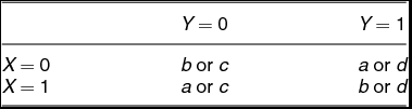
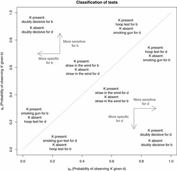

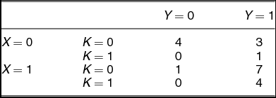
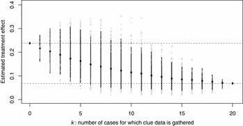

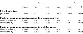
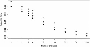
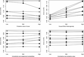




Comments
No Comments have been published for this article.