Prediction uncertainties in the Cape Cod reserving method

Annina Saluz

doi:10.1017/S1748499514000359

Prediction uncertainties in the Cape Cod reserving method

Published online by Cambridge University Press: 18 February 2015

Annina Saluz

Show author details

Annina Saluz*: Affiliation:
Department of Mathematics, RiskLab, ETH Zurich, 8092 Zurich, Switzerland
*: *Correspondence to: Annina Saluz, Department of Mathematics, RiskLab, ETH Zurich, 8092 Zurich, Switzerland. Tel: +41 44 632 68 30; Fax: +41 44 632 15 23; E-mail: annina.saluz@math.ethz.ch

Article contents

Abstract
Introduction
Stochastic model for the CC method
Example
Conclusion
References

Rights & Permissions

Abstract

The Cape Cod (CC) method was designed by Bühlmann and Straub in order to overcome some shortcomings of the chain ladder (CL) method. Owing to its simplicity and because of the advantages over the CL method, the CC method has become a well-established method in practice. In this paper we consider a distribution-free stochastic model for the CC method. Within this model we give the parameter estimates and we derive estimates for the conditional mean square error of prediction for the CC method. In addition, we derive an estimate for the uncertainty in the claims development result.

Keywords

Cape Cod method Claims reserving Mean square error of prediction Claims development result

Information

Type: Papers
Information: Annals of Actuarial Science , Volume 9 , Issue 2 , September 2015, pp. 239 - 263
DOI: https://doi.org/10.1017/S1748499514000359 [Opens in a new window]
Copyright: © Institute and Faculty of Actuaries 2015

1. Introduction

The Cape Cod (CC) method was developed by Bühlmann & Straub (Reference Bühlmann and Straub1983). A derivation of the CC method is published in Straub (Reference Straub1988). In the CC method the reserve of an accident year is the product of an estimate of the expected ultimate claim and the estimated “still-to-come” factor of the corresponding accident year. The estimate of the expected ultimate claim is the product of the premium and an estimate for the loss ratio. For the estimation of the “still-to-come” factor, it is further assumed that there is a development pattern, which is the same for all accident years. Hereby, the development pattern describes the proportion of claims that evolve up to a certain development year relative to the ultimate claim amount.

The CC method was designed in order to overcome some shortcomings of the chain ladder (CL) method, which is one of the most popular claims reserving methods. The CL predictor of the ultimate claim is obtained by multiplying the current claims amount of an accident year (i.e. the claims amount known so far) by a product of development factors. Hence, the CL predictors of the ultimate claims are directly proportional to the current claims amount and therefore, if the current claims amount is zero or an outlier, the CL prediction gives unsatisfactory results. This is in particular the case for long-tailed lines of business in recent accident years. Moreover, the CL method is very sensitive to changes in individual claim numbers. Finally, the CL method is purely based on the claims data and it disregards the information in the premiums. These shortcomings are addressed by the CC method. The CC method is more robust than the CL method and, in contrast to the CL method, the CC method incorporates the information contained in the premiums.

The CC method is also closely related to the Bornhuetter–Ferguson (BF) method (Bornhuetter & Ferguson, Reference Bornhuetter and Ferguson1972). As in the CC method, the BF reserve of an accident year is the product of an estimate of the expected ultimate claim and the estimated “still-to-come” factor of the corresponding accident year. For the estimation of the latter one also assumes that there is a development pattern, which is the same for all accident years. The estimate of the expected ultimate claim is given by an unbiased a priori estimate. The a priori estimate is assumed to be independent from the data of the corresponding accident year and it is not adjusted during the claims development. Often the a priori estimate is the product of the earned premium and an a priori estimate for the loss ratio. On the other hand, the loss ratio in the CC method is estimated from the data and hence it depends on the claims development. In the past, the development pattern for the BF method was often estimated by the development pattern resulting from the CL method. However, Mack (Reference Mack2006) criticises the use of the CL development pattern in the BF method, because the CL method assumes a multiplicative connection between past and future loss amounts, whereas the BF method establishes an additive connection (independence). Moreover, the incorporation of the a priori estimates in the BF method is a fundamental difference to the CL method. Hence, Saluz et al. (Reference Saluz, Gisler and Wüthrich2011) argue that this additional information should also be incorporated in the estimates of the development pattern and that the use of the CL development pattern is inconsistent with the BF philosophy.

In a numerical example Bühlmann & Straub (Reference Bühlmann and Straub1983) use the CL development pattern for the CC method. However, they remark that the estimation of the development pattern is still unsolved. Similar to the BF method, we think that an estimate of the development pattern for the CC method should incorporate the additional information available from the premiums, too.

Owing to its simplicity, the CC method is a well-established method in practice. However, in current literature there is no formula for the estimation of the prediction uncertainty in the CC method (see Dal Moro & Lo, Reference Dal Moro and Lo2014). In this paper we consider a stochastic model for the CC method and we derive estimates for the development pattern within this model. The incorporation of the information from the premiums in the estimation of the development pattern is consistent with our model assumptions. In order to quantify prediction uncertainty we derive an estimate for the conditional mean square error of prediction (MSEP) of the CC reserve and we give an estimate for the uncertainty in the one-year claims development result (CDR).

Organisation of the paper: in the remainder of this section we introduce the notation and we review the CC, CL and BF method. In section 2, we consider a distribution-free model for the CC method. In this model we calculate a development pattern that incorporates the information from the premiums and we derive estimates for the prediction uncertainty of the ultimate claim and for the uncertainty in the CDR. In section 2.2, we consider a distributional model and we show that in this special case the parameter estimates given in the distribution-free model can be derived with maximum likelihood (ML) estimation. A numerical example is given in section 3.

1.1. Notation and data structure

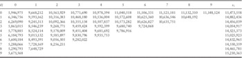
We denote the cumulative claims (cumulative payments or incurred losses) in accident year i∈{0, … , I} at the end of development year j∈{0, … , J} by C _i,j>0 and we assume J≤I. Let X _i,j=C _i,j−C _i,j−1 denote the incremental claims, where we set C _i,−1=0. The summation over an index starting from 0 is denoted with a square bracket, for example:

$$C_{{[k],j}} \,=\,\mathop{\sum}\limits_{i\,=\,0}^k {C_{{i,j}} ,} \quad 0\leq k\leq I,\quad 0\leq j\leq J.$$

We assume that all claims are settled after development year J and therefore the total ultimate claim of accident year i is given by C _i,J. At time I we have information in the upper left trapezoid/triangle:

$${\cal D}_{I} \,=\,\left\{ {C_{{i,j}} :i{\plus}j\leq I,\;j\leq J} \right\},$$

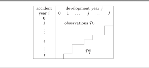
and our goal is to predict the lower right triangle $${\cal D}_{I}^{c} \,=\,\{ C_{{i,j}} :i{\plus}j\,\gt \,I,i\leq I,\;j\leq J\} $$ . An illustration of the data is given in Table 1.

Table 1

Claims development triangle.

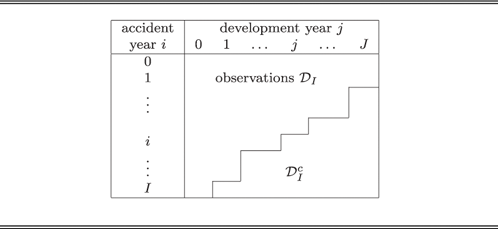
The observations are given in the upper left triangle/trapezoid ${\cal D}_{I} $ . The lower right triangle ${\cal D}_{I}^{c} $ needs to be predicted.

We define the outstanding loss liabilities for accident year i at time I by

(1.1)

$$R_{i} \,=\,C_{{i,J}} {\minus}C_{{i,I{\minus}i}} \,=\,\mathop{\sum}\limits_{j\,=\,I{\minus}i{\plus}1}^J {X_{{i,j}} ,} \quad I{\minus}J{\plus}1\leq i\leq I,$$

and the total outstanding loss liabilities are defined by $$R=\mathop{\sum}\nolimits_{i\,=\,I{\minus}J{\plus}1}^I {R_{i} } $$ . For accident years i=0, … , I−J the ultimate claim C _i,J is known at time I and hence R _i=0, i=0, … , I−J.

Remark 1.1 If C _i,j denote cumulative payments then formula (1.1) gives the “true” outstanding loss liabilities. For incurred losses C _i,j the “true” outstanding loss liabilities are given by

(1.2)

$$\bar{R}_{i} \,=\,C_{{i,J}} {\minus}C_{{i,I{\minus}i}} {\plus}C_{{i,I{\minus}i}} {\minus}C_{{i,I{\minus}i}}^{{{\rm paid}}}, \quad I{\minus}J{\plus}1\leq i\leq I,$$

with $$C_{{i,j}}^{{{\rm paid}}} $$ denoting the cumulative payments of accident year i up to development year j. Note that the additional term $$C_{{i,I{\minus}i}} {\minus}C_{{i,I{\minus}i}}^{{{\rm paid}}} $$ is observable at time I and has no impact on the claims prediction problem. Therefore, we only consider the outstanding loss liabilities as defined in (1.1).

The budgeting and planning process in an insurance company gives information on the premium level of each accident year. Often premium levels are adjusted to business cycles. For instance, in soft markets, the premium level is often increased by a certain percentage. We denote the earned on-level premium for accident year i by ν _i, 0≤i≤I. This means that ν _i is the earned premium, adjusted for business cycles, such that the expected loss ratio is the same for all accident years. These adjustments are based on the information from the budgeting and planning process, which should be available in a company. In periods of a stable premium level, the earned premiums can be used for the on-level premiums ν _i. Otherwise, if it is for instance known that the premiums of an accident year are increased by a certain percentage owing to soft market conditions, then the on-level premiums are corrected for this increase. Mack (Reference Mack2006) also derives a procedure for the calculation of on-level premiums from the data. However, with the procedure of Mack (Reference Mack2006) the resulting on-level premiums depend on the data $${\cal D}_{I} $$ . Here, we assume that the calculation of the v _i’s does not incorporate the data in the triangle and that the v _i’s can be considered as known constants.

In order to simplify notation we denote the index of the last observed development year in accident year i by $$\iota (i)=\min (I{\minus}i,J)$$ .

1.2. CL method

The CL prediction of the ultimate claim C _i,J of accident year i>I−J is given by

(1.3)

$$\hat{C}_{{i,J}}^{{{\rm CL}}} \,=\,C_{{i,\iota (i)}} \prod\limits_{j\,=\,\iota (i)}^{J{\minus}1} {\hat{f}_{j} ,} \quad {\rm where}\quad \hat{f}_{j} \,=\,{{C_{{[I{\minus}j{\minus}1],j{\plus}1}} } \over {C_{{[I{\minus}j{\minus}1],j}} }}.$$

The CL reserve is given by

$$\eqalignno{ \hat{R}_{i}^{{{\rm CL}}} & \,=\,C_{{i,\iota (i)}} \left( {\prod\limits_{j\,=\,\iota (i)}^{J{\minus}1} {\hat{f}_{j} {\minus}1} } \right)=C_{{i,\iota (i)}} \prod\limits_{j\,=\,\iota (i)}^{J{\minus}1} {\hat{f}_{j} } \left( {1{\minus}\prod\limits_{j\,=\,\iota (i)}^{J{\minus}1} {\hat{f}_{j}^{{{\minus}1}} } } \right) \cr & \,=\,\hat{C}_{{i,J}}^{{{\rm CL}}} \left( {1{\minus}\hat{\beta }_{{\iota (i)}}^{{{\rm CL}}} } \right). $$

The CL development pattern

(1.4)

$$\hat{\beta }_{j}^{{{\rm CL}}} \,=\,\prod\limits_{k\,=\,j}^{J{\minus}1} {\hat{f}_{k}^{{{\minus}1}} ,} \quad 0\leq j\leq J{\minus}1,\quad \hat{\beta }_{J}^{{{\rm CL}}} \,=\,1,$$

is an estimate of the development pattern β _j, 0≤j≤J, which describes the percentage of claims that evolve up to development year j relative to the ultimate claim.

There are different stochastic models that justify the use of the CL algorithm. A distribution-free model was suggested by Mack (Reference Mack1993).

As mentioned above, the proportionality of the CL predictor to the current claims amount C _i,ι(i) is sometimes problematic in long-tailed lines of business for recent accident years. Note that the $$\hat{f}_{j} $$ for late development years are based on few observations. A change of C _0,J has a multiplicative impact on the prediction of the ultimate claims of all accident years. Therefore, the CL method is very sensitive to changes of individual numbers.

1.3. CC method

The CC predictor (see Bühlmann & Straub, Reference Bühlmann and Straub1983) for the ultimate claim C _i,J is given by

(1.5)

$$\hat{C}_{{i,J}}^{{{\rm CC}}} \,=\,C_{{i,\iota (i)}} {\plus}\nu _{i} \hat{q}\left( {1{\minus}\hat{\beta }_{{\iota (i)}} } \right),$$

where

(1.6)

$$\hat{q}={{\mathop{\sum}\nolimits_{i\,=\,0}^I {C_{{i,\iota (i)}} } } \over {\mathop{\sum}\nolimits_{i\,=\,0}^I {\nu _{i} \hat{\beta }_{{\iota (i)}} } }}.$$

Moreover, $$\hat{\beta }_{{\iota (i)}} $$ is an estimate of β _ι(i). As above, the development pattern β _j, 0≤j≤J, describes the percentage of claims that evolve up to development year j relative to the ultimate claim. Note that for each i

$$\hat{q}_{i} \,=\,{{C_{{i,\iota (i)}} } \over {\nu _{i} \hat{\beta }_{{\iota (i)}} }}$$

is an estimate for the loss ratio q and hence $$\hat{q}$$ is a weighted average loss ratio with the weights $$\nu _{i} \hat{\beta }_{{\iota (i)}} $$ .

In the original article of Bühlmann & Straub (Reference Bühlmann and Straub1983) it is mentioned that the estimation of the development pattern $${\beta }_{j} $$ is an unsolved problem. In practice the development pattern is often estimated by the CL development pattern given in (1.4). In this case the CC predictor of the ultimate claim can be written as

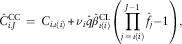$$\hat{C}_{{i,J}}^{{{\rm CC}}} \,=\,C_{{i,\iota (i)}} {\plus}\nu _{i} \hat{q}\hat{\beta }_{{\iota (i)}}^{{{\rm CL}}} \left( {\prod\limits_{j\,=\,\iota (i)}^{J{\minus}1} {\hat{f}_{j} {\minus}1} } \right),$$

that is, we replace the diagonal element C _i,ι(i) in the CL prediction

$$\hat{C}_{{i,J}}^{{{\rm CL}}} \,=\,C_{{i,\iota (i)}} \prod\limits_{j\,=\,\iota (i)}^{J{\minus}1} {\hat{f}_{j} } \,=\,C_{{i,\iota (i)}} {\plus}C_{{i,\iota (i)}} \left( {\prod\limits_{j\,=\,\iota (i)}^{J{\minus}1} {\hat{f}_{j} {\minus}1} } \right),$$

by the more robust value

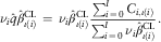$$\nu _{i} \hat{q}\hat{\beta }_{{\iota (i)}}^{{{\rm CL}}} \,=\,\nu _{i} \hat{\beta }_{{\iota (i)}}^{{{\rm CL}}} {{\mathop{\sum}\nolimits_{i\,=\,0}^I {C_{{i,\iota (i)}} } } \over {\mathop{\sum}\nolimits_{i\,=\,0}^I {\nu _{i} \hat{\beta }_{{\iota (i)}}^{{{\rm CL}}} } }}.$$

Therefore, one can interpret the CC method as an application of the CL algorithm to these more robust diagonal values (see Wüthrich & Merz, Reference Wüthrich and Merz2008). On the other hand, if we take formula (1.5), the CC method is close to the BF method in which the predictor of the ultimate claim is given by

(1.7)

$$\hat{C}_{{i,J}}^{{{\rm BF}}} \,=\,C_{{i,\iota (i)}} {\plus}\hat{\mu }_{i} \left( {1{\minus}\hat{\beta }_{{\iota (i)}} } \right),$$

where $$\hat{\mu }_{i} $$ is an unbiased a priori estimate of the expected ultimate claim E[C _i,J]. In the BF method $$\hat{\mu }_{i} $$ is usually an estimate that incorporates information from the earned premiums p _i. In this case it is assumed that for each accident year an a priori estimate for the loss ratio $$\hat{q}_{i} $$ is available and $$\hat{\mu }_{i} \,=\,p_{i} \hat{q}_{i} $$ . The loss ratio estimates $$\hat{q}_{i} $$ are typically assumed to be independent from the data of the corresponding accident year i (see, for instance Mack, Reference Mack2008; Alai et al., Reference Alai, Merz and Wüthrich2010; Saluz et al., Reference Saluz, Gisler and Wüthrich2011). These a priori estimates $$\hat{q}_{i} $$ are known at the beginning of each accident year and they are not adjusted during the claims development. In contrast to the BF method, the loss ratio q in the CC method is estimated from the data $${\cal D}_{I} $$ . Moreover, the CC method assumes a constant loss ratio, which means that the earned premiums p _i need to be adjusted to on-level premiums v _i. Instead of assuming the availability of unbiased a priori estimates of E[C _i,J], the CC method assumes that the expected ultimate claims are known up to a constant factor. In the BF predictor (1.7) we further note the additive relation with the current claims amount C _i,ι(i). This additive relation leads to a reserve estimate:

$$\hat{R}_{i}^{{{\rm BF}}} \,=\,\hat{\mu }_{i} (1{\minus}\hat{\beta }_{{I{\minus}i}} ),$$

which does not directly depend on C _i,ι(i). The BF method typically assumes independence between past and future claims (see Mack, Reference Mack2008). In contrast, the CL predictor given in (1.3) and the corresponding reserve are directly proportional to C _i,ι(i). Owing to this different relation (additive or multiplicative), Mack (Reference Mack2006) criticises the use of the CL development pattern in the BF method and suggests different estimates. Saluz et al. (Reference Saluz, Gisler and Wüthrich2011) argue that the information from the a priori estimates should be incorporated in the estimation of the development pattern in the BF method and derive corresponding estimators based on ML considerations. For the CC method we suggest similar estimators that incorporate the premiums ν _i. The suggested estimators are derived from the best linear unbiased estimators. In section 2.2 it will be seen that under the assumption that incremental claims are overdispersed Poisson (ODP) distributed, these estimators coincide with the ML estimators.

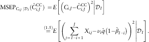
In order to quantify the uncertainties in the CC predictions we will consider second moments. The conditional MSEP for accident year i>I−J, given $${\cal D}_{I} $$ , is given by

$$\eqalignno{ {\rm MSEP}_{{C_{{i,J}} \,\mid\,{\cal D}_{I} }} (\hat{C}_{{i,J}}^{{{\rm CC}}} )\,= \,& E\left[ {\left. {\left( {C_{{i,J}} {\minus}\hat{C}_{{i,J}}^{{{\rm CC}}} } \right)^{2} } \right|{\cal D}_{I} } \right] \cr \mathop{=}\limits^{{(1.5)}} & E\left[ {\left. {\left( {\mathop{\sum}\limits_{j\,=\,I{\minus}i{\plus}1}^J {X_{{i,j}} } {\minus}\nu _{i} \hat{q}\left( {1{\minus}\hat{\beta }_{{I{\minus}i}} } \right)} \right)^{2} } \right|{\cal D}_{I} } \right]. $$

Similarly, for aggregated accident years we want to estimate

$${\rm MSEP}_{{\mathop{\sum}\nolimits_{i\,=\,I{\minus}J{\plus}1}^I {C_{{i,J}} \,\mid\,{\cal D}_{I} } }} \left( {\mathop{\sum}\limits_{i\,=\,I{\minus}J{\plus}1}^I {\hat{C}_{{i,J}}^{{{\rm CC}}} } } \right)=E\left[ {\left. {\left( {\mathop{\sum}\limits_{i\,=\,I{\minus}J{\plus}1}^I {\left( {C_{{i,J}} {\minus}\hat{C}_{{i,J}}^{{{\rm CC}}} } \right)} } \right)^{2} } \right|{\cal D}_{I} } \right].$$

In order to estimate the conditional MSEP a stochastic model will be introduced in the following section.

2. Stochastic model for the CC method

2.1. CC method in a distribution-free model

For the estimation of the prediction uncertainty in the CC method we assume the following underlying distribution-free model.

Model Assumptions 2.1 (CC model) Incremental claims X _i,j are independent and there exist positive parameters q, σ _j², 0≤j≤J, and a development pattern γ ₀, … , γ _J, with $$\mathop{\sum}\nolimits_{j\,=\,0}^J \gamma _{j} \,=\,1$$ such that

$$E[X_{{i,j}} ]=\nu _{i} q\gamma _{j} \quad {\rm and}\quad {\rm Var}(X_{{i,j}} )=\nu _{i} q\sigma _{j}^{2} $$

for 0≤i≤I and 0≤j≤J.

Note that γ _j denotes the incremental development pattern γ _j=β _j−β _j−1, 1≤j≤J, and γ ₀=β ₀. Further, we remark that the expected loss ratio q is the same for all accident years. This means that the premiums ν _i are “on-level” premiums as explained below Remark 1.1.

2.1.1. Parameter estimation

Under Model Assumptions 2.1 the best linear unbiased estimate for γ _j is given by

$$\tilde{\gamma }_{j}^{{{\rm raw}}} \,=\,{{X_{{[I{\minus}j],j}} } \over {q\nu _{{[I{\minus}j]}} }}.$$

In general, the $$\tilde{\gamma }_{j}^{{{\rm raw}}} $$ ’s do not sum up to 1 and hence we consider the normalised development pattern

$$\hat{\gamma }_{j} \,=\,{{\tilde{\gamma }_{j}^{{{\rm raw}}} } \over {\mathop{\sum}\nolimits_{k\,=\,0}^J {\tilde{\gamma }_{k}^{{{\rm raw}}} } }}.$$

Note that the normalised development pattern $$\hat{\gamma }_{j} $$ does not depend on the unknown loss ratio q, that is, we have

(2.1)

$$\hat{\gamma }_{j} \,=\,{{\tilde{\gamma }_{j}^{{{\rm raw}}} } \over {\mathop{\sum}\nolimits_{k\,=\,0}^J {\tilde{\gamma }_{k}^{{{\rm raw}}} } }}={{\hat{\gamma }_{j}^{{{\rm raw}}} } \over {\mathop{\sum}\nolimits_{k\,=\,0}^J {\hat{\gamma }_{k}^{{{\rm raw}}} } }}={{\hat{\gamma }_{j}^{{{\rm raw}}} } \over {\hat{\beta }_{J}^{{{\rm raw}}} }},$$

where

(2.2)

$$\hat{\gamma }_{j}^{{{\rm raw}}} \,=\,{{X_{{[I{\minus}j],j}} } \over {\nu _{{[I{\minus}j]}} }}$$

and 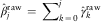$$\hat{\beta }_{j}^{{{\rm raw}}} \,=\,\mathop{\sum}\nolimits_{k\,=\,0}^j \hat{\gamma }_{k}^{{{\rm raw}}} $$ . The cumulative development pattern β _j is then estimated by

(2.3)

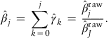$$\hat{\beta }_{j} \,=\,\mathop{\sum}\limits_{k\,=\,0}^j {\hat{\gamma }_{k} } \,=\,{{\hat{\beta }_{j}^{{{\rm raw}}} } \over {\hat{\beta }_{J}^{{{\rm raw}}} }}.$$

The best linear unbiased estimator for q based on the observations X _i,j, i+j≤I, j≤J, is given by

(2.4)

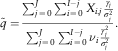$$\tilde{q}={{\mathop{\sum}\nolimits_{j\,=\,0}^J {\mathop{\sum}\nolimits_{i\,=\,0}^{I{\minus}j} {X_{{i,j}} {{\gamma _{j} } \over {\sigma _{j}^{2} }}} } } \over {\mathop{\sum}\nolimits_{j\,=\,0}^J {\mathop{\sum}\nolimits_{i\,=\,0}^{I{\minus}j} {\nu _{i} {{\gamma _{j}^{2} } \over {\sigma _{j}^{2} }}} } }}.$$

If we insert the estimates (2.1) for the γ _j’s in $$\tilde{q}$$ we obtain

(2.5)

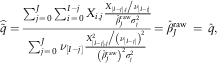$$\widehat{{\tilde{q}}}={{\mathop{\sum}\nolimits_{j\,=\,0}^J {\mathop{\sum}\nolimits_{i\,=\,0}^{I{\minus}j} {X_{{i,j}} } } {{{{X_{{[I{\minus}j],j}} } \mathord{\left/ {\vphantom {{X_{{[I{\minus}j],j}} } {\nu _{{[I{\minus}j]}} }}} \right. \kern-\nulldelimiterspace} {\nu _{{[I{\minus}j]}} }}} \over {\hat{\beta }_{J}^{{{\rm raw}}} \sigma _{j}^{2} }}} \over {\mathop{\sum}\nolimits_{j\,=\,0}^J {\nu _{{[I{\minus}j]}} } {{{{X_{{[I{\minus}j],j}}^{2} } \mathord{\left {\scriptstyle \big/} {\vphantom {{X_{{[I{\minus}j],j}}^{2} } {\left( {\nu _{{[I{\minus}j]}} } \right)^{2} }}} \right. \kern-\nulldelimiterspace} {\left( {\nu _{{[I{\minus}j]}} } \right)^{2} }}} \over {\left( {\hat{\beta }_{J}^{{{\rm raw}}} } \right)^{2} \sigma _{j}^{2} }}}}=\hat{\beta }_{J}^{{{\rm raw}}} \,=\,\hat{q},$$

where $$\hat{q}$$ was defined in (1.6). The third equality in (2.5) is derived as follows:

(2.6)

$$\eqalignno{ \hat{q}\mathop{=}\limits^{{(1.6)}} & {{\mathop{\sum}\nolimits_{i\,=\,0}^I {C_{{i,\iota (i)}} } } \over {\mathop{\sum}\nolimits_{i\,=\,0}^I {\nu _{i} \hat{\beta }_{{\iota (i)}} } }}\mathop{=}\limits^{{(2.1)}} {{\mathop{\sum}\nolimits_{i\,=\,0}^I {C_{{i,\iota (i)}} } } \over {\mathop{\sum}\nolimits_{\scriptstyle i{\plus}j\leq I, \hfill \atop \scriptstyle j\leq J \hfill} {\nu _{i} } {{{{X_{{[I{\minus}j],j}} } \mathord{\left/ {\vphantom {{X_{{[I{\minus}j],j}} } {\nu _{{[I{\minus}j]}} }}} \right. \kern-\nulldelimiterspace} {\nu _{{[I{\minus}j]}} }}} \over {\hat{\beta }_{J}^{{{\rm raw}}} }}}} \cr & \hskip-14pt=\, {{\hat{\beta }_{J}^{{{\rm raw}}} \mathop{\sum}\nolimits_{j\,=\,0}^J {X_{{[I{\minus}j],j}} } } \over {\mathop{\sum}\nolimits_{j\,=\,0}^J {\nu _{{[I{\minus}j]}} } {{X_{{[I{\minus}j],j}} } \over {\nu _{{[I{\minus}j]}} }}}}=\hat{\beta }_{J}^{{{\rm raw}}} \,=\,\widehat{{\tilde{q}}} .$$

Hence, in the CC model 2.1 the use of the CC loss ratio estimate (1.6) can be justified by a derivation from the best linear unbiased estimate of q. Under Model Assumptions 2.1 we therefore use the following estimates

(2.7)

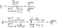$$\eqalignno{ \hat{\gamma }_{j} \,=\, & {{{{X_{{[I{\minus}j],j}} } \over {\nu _{{[I{\minus}j]}} }}} \over {\mathop{\sum}\nolimits_{l=0}^J {{{X_{{[I{\minus}l],l}} } \over {\nu _{{[I{\minus}l]}} }}} }}={{\hat{\gamma }_{j}^{{{\rm raw}}} } \over {\hat{\beta }_{J}^{{{\rm raw}}} }},\quad \quad \cr \hat{q}= & {{\mathop{\sum}\nolimits_{i\,=\,0}^I {C_{{i,\iota (i)}} } } \over {\mathop{\sum}\nolimits_{i\,=\,0}^I {\nu _{i} \hat{\beta }_{{\iota (i)}} } }}=\mathop{\sum}\limits_{l=0}^J {{{X_{{[I{\minus}l],l}} } \over {\nu _{{[I{\minus}l]}} }}} \,=\,\hat{\beta }_{J}^{{{\rm raw}}}. $$

Note that the loss ratio $$\hat{q}$$ corresponds to the multiplicative normalisation factor $$\hat{\beta }_{J}^{{{\rm raw}}} $$ of the non-normalised development pattern given in (2.2). For the CC reserve and ultimate prediction for accident years i>I−J we then have

(2.8)

$$\hat{R}_{i}^{{{\rm CC}}} \,=\,\nu _{i} \hat{q}(1{\minus}\hat{\beta }_{{I{\minus}i}} )=\nu _{i} \hat{\beta }_{J}^{{{\rm raw}}} \left(1{\minus}{{\hat{\beta }_{{I{\minus}i}}^{{{\rm raw}}} } \over {\hat{\beta }_{J}^{{{\rm raw}}} }}\right)=\nu _{i} (\hat{\beta }_{J}^{{{\rm raw}}} {\minus}\hat{\beta }_{{I{\minus}i}}^{{{\rm raw}}} ),$$

(2.9)

$$\hat{C}_{{i,J}}^{{{\rm CC}}} \,=\,C_{{i,I{\minus}i}} {\plus}\hat{R}_{i}^{{{\rm CC}}}.$$

From (2.8) we note that the loss ratio estimate $$\hat{q}$$ in $$\hat{R}_{i}^{{{\rm CC}}} $$ can be omitted if the development pattern is not normalised.

Remark 2.2

∙ In order to incorporate a tail development $$\hat{\gamma }_{{J{\plus}1}} $$ one should normalise the raw development pattern $$\hat{\gamma }_{j}^{{{\rm raw}}} $$ such that for the normalised development pattern $$\hat{\gamma }_{j} \,=\,\hat{\gamma }_{j}^{{{\rm raw}}} /c$$ we obtain

$$\mathop{\sum}\limits_{j\,=\,0}^J \hat{\gamma }_{j} \,=\,\mathop{\sum}\limits_{j\,=\,0}^J {{{\hat{\gamma }_{j}^{{{\rm raw}}} } \over c}} \,=\,{{\hat{\beta }_{J}^{{{\rm raw}}} } \over c}=\hat{\beta }_{J} \,=\,1{\minus}\hat{\gamma }_{{J{\plus}1}}, $$

where c denotes the normalising constant. Therefore, we obtain $$\hat{\gamma }_{j} \,=\,\hat{\gamma }_{j}^{{{\rm raw}}} /c=\hat{\gamma }_{j}^{{{\rm raw}}} (1{\minus}\hat{\gamma }_{{J{\plus}1}} )/\hat{\beta }_{J}^{{{\rm raw}}} $$ . Inserting $$\hat{\gamma }_{j} $$ in (2.4) one gets the estimate

$$\hat{q}={{\hat{\beta }_{J}^{{{\rm raw}}} } \over {1{\minus}\hat{\gamma }_{{J{\plus}1}} }}.$$

For the reserves one obtains in this case:

$$\hat{R}_{i}^{{{\rm CC}}} \,=\,\nu _{i} \hat{q}\left( {1{\minus}\hat{\beta }_{{I{\minus}i}} } \right)=\nu _{i} \left( {{{\hat{\beta }_{J}^{{{\rm raw}}} } \over {1{\minus}\hat{\gamma }_{{J{\plus}1}} }}{\minus}\hat{\beta }_{{I{\minus}i}}^{{{\rm raw}}} } \right).$$

Here, the tail development $$\hat{\gamma }_{{J{\plus}1}} $$ is assumed to be given by an expert.

∙ The representation (2.8) of the CC reserve with the non-normalised development pattern $$\hat{\beta }_{J}^{{{\rm raw}}} $$ substantially simplifies the analysis of prediction uncertainty. For instance, for the non-normalised development pattern one can explicitly calculate the covariances $${\rm Cov}(\hat{\beta }_{j}^{{{\rm raw}}} ,\hat{\beta }_{k}^{{{\rm raw}}} )$$ , 0≤j, k≤J. For the normalised development pattern this is not possible because of the random variables in the denominators.
∙ In the BF method the estimation of the development pattern suggested by Mack (Reference Mack2008) is also based on estimators of the form

$$\tilde{\gamma }_{j}^{{{\rm raw}}} \,=\,{{X_{{[I{\minus}j],j}} } \over {\mu _{{[I{\minus}j]}} }},\quad {\rm where}\quad \mu _{i} \,=\,E[C_{{i,J}} ],\quad 0\leq i\leq I.$$

However, the unknown μ _i are replaced by the a priori estimates $$\hat{\mu }_{i} $$ , which possibly incorporate non-constant a priori loss ratios $$\hat{q}_{i} $$ . In contrast to CC, the BF reserve cannot be rewritten as simply as the CC reserve (2.8). For BF, a normalised development pattern has to be used. Moreover, in the prediction error of the BF reserve the uncertainties in the a priori estimates need to be incorporated.

For the estimation of the conditional MSEP we further need estimates for qσ _j². Denote by Y _i,j the “incremental loss ratios” Y _i,j=X _i,j/ν _i. Observe that

$${\rm Var}(Y_{{i,j}} )={{q\sigma _{j}^{2} } \over {\nu _{i} }},$$

and qσ _j² is the variance of Y _i,j per unit of ν _i. An unbiased estimator for qσ _j², j≠I, is given by

(2.10)

$$\widehat{{q\sigma ^{2} }}_{j} \,=\,{1 \over {I{\minus}j}}\mathop{\sum}\limits_{i\,=\,0}^{I{\minus}j} {\nu _{i} } \left( {{{X_{{i,j}} } \over {\nu _{i} }}{\minus}\hat{\gamma }_{j}^{{{\rm raw}}} } \right)^{2} ,\quad 0\leq j\leq J,\;j\,\ne\,I.$$

In the case where I=J an estimate for qσ _J² is obtained with the extrapolation from Mack (Reference Mack1993):

$$\eqalignno{ \widehat{{q\sigma _{J}^{2} }}= & \min \left( {\widehat{{q\sigma ^{2} }}_{{J{\minus}1}} ,\,\widehat{{q\sigma ^{2} }}_{{J{\minus}2}} ,\,{{\widehat{{q\sigma ^{2} }}_{{J{\minus}1}}^{2} } \over {\widehat{{q\sigma ^{2} }}_{{J{\minus}2}} }}} \right) \,=\, \min \left( {\widehat{{q\sigma ^{2} }}_{{J{\minus}2}} ,\,{{\widehat{{q\sigma ^{2} }}_{{J{\minus}1}}^{2} } \over {\widehat{{q\sigma ^{2} }}_{{J{\minus}2}} }}} \right). $$

2.1.1. Prediction uncertainty

Under Model Assumptions 2.1 we have for the conditional MSEP of accident year i>I−J, given $${\cal D}_{I} $$ :

(2.11)

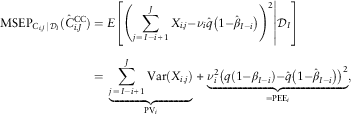$$\eqalignno{ {\rm MSEP}_{{C_{{i,J}} \,\mid\,{\cal D}_{I} }} (\hat{C}_{{i,J}}^{{{\rm CC}}} )&=E\left[ {\left. {\left( {\mathop{\sum}\limits_{j\,=\,I{\minus}i{\plus}1}^J {X_{{i,j}} } {\minus}\nu _{i} \hat{q}\left( {1{\minus}\hat{\beta }_{{I{\minus}i}} } \right)} \right)^{2} } \right|{\cal D}_{I} } \right] \cr & =\,\mathop{\underbrace{{\mathop{\sum}\limits_{j\,=\,I{\minus}i{\plus}1}^J {\rm Var}(X_{{i,j}} )}}}\limits_{{\rm PV}_{i} }{\plus}\mathop{\underbrace{{\nu _{i}^{2} \left( {q\left( {1{\minus}\beta _{{I{\minus}i}} } \right){\minus}\hat{q}\left( {1{\minus}\hat{\beta }_{{I{\minus}i}} } \right)} \right)^{2} }}}\limits_{={\rm PEE}_{i} }, $$

where PV_i is the process variance of accident year i, which describes the randomness of the X _i,j, and PEE_i the parameter estimation error, which describes the uncertainties in the parameter estimates. The conditional MSEP can be estimated as follows:

Estimate 2.3 (MSEP, CC model) Under Model Assumptions 2.1 the conditional MSEP of the CC predictor $$\hat{C}_{{i,J}}^{{{\rm CC}}} $$ given in (2.9) is estimated by

$$\widehat{{{\rm MSEP}}}_{{C_{{i,J}} \,\mid\,{\cal D}_{I} }} \left( {\hat{C}_{{i,J}}^{{{\rm CC}}} } \right)=\widehat{{{\rm PV}}}_{i} {\plus}\widehat{{{\rm PEE}}}_{i} ,$$

where $$\widehat{{{\rm PV}}}_{i} $$ and $$\widehat{{{\rm PEE}}}_{i} $$ are given by

(2.12)

$$\widehat{{{\rm PV}}}_{i} \,=\,\mathop{\sum}\limits_{j\,=\,I{\minus}i{\plus}1}^J {\nu _{i} \widehat{{q\sigma ^{2} }}_{j} ,} \quad \widehat{{{\rm PEE}}}_{i} \,=\,\nu _{i}^{2} \mathop{\sum}\limits_{j\,=\,I{\minus}i{\plus}1}^J {{{\widehat{{q\sigma ^{2} }}_{j} } \over {\nu _{{[I{\minus}j]}} }}}, $$

and where $$\widehat{{q\sigma ^{2} }}_{j} $$ is given in (2.10). For aggregated accident years the corresponding conditional MSEP is estimated by

$$\widehat{{{\rm MSEP}}}_{{\mathop{\sum}\nolimits_{i\,=\,I{\minus}J{\plus}1}^I {C_{{i,J}} \,\mid\,{\cal D}_{I} } }} \left( {\mathop{\sum}\limits_{i\,=\,I{\minus}J{\plus}1}^I {\hat{C}_{{i,J}}^{{{\rm CC}}} } } \right)=\mathop{\sum}\limits_{i\,=\,I{\minus}J{\plus}1}^I {\widehat{{{\rm MSEP}}}_{{C_{{i,J}} \,\mid\,{\cal D}_{I} }} \left( {\hat{C}_{{i,J}}^{{{\rm CC}}} } \right)} {\plus}2\mathop{\sum}\limits_{I{\minus}J{\plus}1\leq i\lt k\leq I} {\widehat{{{\rm PEE}}}_{{i,k}} }, $$

where $$\widehat{{{\rm PEE}}}_{{i,k}} $$ is given by

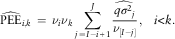$$\widehat{{{\rm PEE}}}_{{i,k}} \,=\,\nu _{i} \nu _{k} \mathop{\sum}\limits_{j\,=\,I{\minus}i{\plus}1}^J {{{\widehat{{q\sigma ^{2} }}_{j} } \over {\nu _{{[I{\minus}j]}} }},} \quad i\lt k.$$

The derivation of Estimate 2.3 is given in Appendix A.

2.1.2. Conditional MSEP of the one-year CDR

So far we have considered the prediction of the outstanding liabilities at time I. At the end of accounting year I we have an additional diagonal of observations in the claims triangle/trapezoid and the predictions of the ultimate claims are updated according to this new information. The one-year CDR is the difference between two successive predictors of the ultimate claim (see, for instance Merz & Wüthrich, Reference Merz and Wüthrich2008). More precisely, we define the CDR for accounting year I+1 and for accident year i by

(2.13)

$${\rm CDR}_{i}^{{(I{\plus}1)}} \,=\,\hat{C}_{{i,J}}^{{(I)}} {\minus}\hat{C}_{{i,J}}^{{(I{\plus}1)}}, $$

where $$\hat{C}_{{i,J}}^{{(k)}} $$ , k=I, I+1, denotes the prediction of C _i,J at time k. Under the CC model 2.1 we have for I−J+1≤i≤I

(2.14)

$$\hat{C}_{{i,J}}^{{(I)}} \,=\,C_{{i,I{\minus}i}} {\plus}\nu _{i} \hat{q}^{{(I)}} \left( {1{\minus}\hat{\beta }_{{I{\minus}i}}^{{(I)}} } \right)=C_{{i,I{\minus}i}} {\plus}\nu _{i} \left( {\hat{\beta }_{J}^{{(I){\rm raw}}} {\minus}\hat{\beta }_{{I{\minus}i}}^{{(I){\rm raw}}} } \right),$$

(2.15)

$$\hat{C}_{{i,J}}^{{(I{\plus}1)}} \,=\,C_{{i,I{\minus}i{\plus}1}} {\plus}\nu _{i} \hat{q}^{{(I{\plus}1)}} \left( {1{\minus}\hat{\beta }_{{I{\minus}i{\plus}1}}^{{(I{\plus}1)}} } \right)=C_{{i,I{\minus}i{\plus}1}} {\plus}\nu _{i} \left( {\hat{\beta }_{J}^{{(I{\plus}1){\rm raw}}} {\minus}\hat{\beta }_{{I{\minus}i{\plus}1}}^{{(I{\plus}1){\rm raw}}} } \right),$$

where $$\hat{q}^{{(k)}} \,=\,\hat{\beta }_{J}^{{(k){\rm raw}}} $$ , k=I, I+1, and

(2.16)

$$\hat{\beta }_{j}^{{(k){\rm raw}}} \,=\,\mathop{\sum}\limits_{l=0}^j {\hat{\gamma }_{l}^{{(k){\rm raw}}} ,} \quad {\rm with}\quad \hat{\gamma }_{j}^{{(k){\rm raw}}} \,=\,{{X_{{[k{\minus}j],j}} } \over {\nu _{{[k{\minus}j]}} }}.$$

Similarly, we define the CDR for aggregated accident years at time I+1 by

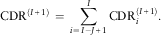$${\rm CDR}^{{(I{\plus}1)}} \,=\,\mathop{\sum}\limits_{i\,=\,I{\minus}J{\plus}1}^I {{\rm CDR}_{i}^{{(I{\plus}1)}} } .$$

At time I we predict CDR_i^(I+1) by 0 as we consider $$\hat{C}_{{i,J}}^{{(I)}} $$ as best estimate based on the available information at time I. New solvency regulations such as the Swiss Solvency Test (FINMA, 2006) require additional risk capital for protection against possible shortfalls in this one-year CDR. In order to quantify uncertainties in the CDRs we consider second moments given by

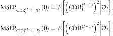$$\eqalignno{ & {\rm MSEP}_{{{\rm CDR}_{i}^{{(I{\plus}1)}} \,\mid\,{\cal D}_{I} }} (0)=E\left[ {\left. {\left( {{\rm CDR}_{i}^{{(I{\plus}1)}} } \right)^{2} } \right|{\cal D}_{I} } \right] ,\cr & {\rm MSEP}_{{{\rm CDR}^{{(I{\plus}1)}} \,\mid\,{\cal D}_{I} }} (0)=E\left[ {\left. {\left( {{\rm CDR}^{{(I{\plus}1)}} } \right)^{2} } \right|{\cal D}_{I} } \right]. $$

In Appendix A the following estimators for these conditional MSEPs are derived:

Estimate 2.4 (MSEP CDR, CC model) Under Model Assumptions 2.1 the conditional MSEP of the CDR of accident year i given in (2.13) is estimated by

$$\widehat{{{\rm MSEP}}}_{{{\rm CDR}_{i}^{{(I{\plus}1)}} \,\mid\,{\cal D}_{I} }} (0)=\nu _{i} \widehat{{q\sigma ^{2} }}_{{I{\plus}1{\minus}i}} {{\nu _{{[i]}} } \over {\nu _{{[i{\minus}1]}} }}{\plus}\nu _{i}^{2} \mathop{\sum}\limits_{j\,=\,I{\plus}2{\minus}i}^J {\widehat{{q\sigma ^{2} }}_{j} } {{\nu _{{I{\plus}1{\minus}j}} } \over {\nu _{{[I{\minus}j]}} \nu _{{[I{\plus}1{\minus}j]}} }},$$

where the $$\widehat{{q\sigma ^{2} }}_{j} $$ ’s are given in (2.10). For aggregated accident years the corresponding conditional MSEP is estimated by

$$\widehat{{{\rm MSEP}}}_{{{\rm CDR}^{{(I{\plus}1)}} \,\mid\,{\cal D}_{I} }} (0)=\!\mathop{\sum}\limits_{i\,=\,I{\minus}J{\plus}1}^I {\widehat{{{\rm MSEP}}}_{{{\rm CDR}_{i}^{{(I{\plus}1)}} \,\mid\,{\cal D}_{I} }} (0){\plus}} 2\mathop{\sum}\limits_{I{\minus}J{\plus}1\leq i\lt k\leq I} {\nu _{i} \nu _{k} } \left( {{{\widehat{{q\sigma ^{2} }}_{{I{\plus}1{\minus}i}} } \over {\nu _{{[i{\minus}1]}} }}{\plus}\mathop{\sum}\limits_{j\,=\,I{\plus}2{\minus}i}^J {{{\widehat{{q\sigma ^{2} }}_{j} \nu _{{I{\plus}1{\minus}j}} } \over {\nu _{{[I{\minus}j]}} \nu _{{[I{\plus}1{\minus}j]}} }}} } \right).$$

In order to compare the formula given in Estimate 2.4 with the formula for the conditional MSEP of the predictor for the ultimate claim given in Estimate 2.3, we rewrite Estimate 2.4 as follows

$$\widehat{{{\rm MSEP}}}_{{{\rm CDR}_{i}^{{(I{\plus}1)}} \,\mid\,{\cal D}_{I} }} (0)=\nu _{i} \widehat{{q\sigma ^{2} }}_{{I{\plus}1{\minus}i}} {\plus}\nu _{i}^{2} {{\widehat{{q\sigma ^{2} }}_{{I{\plus}1{\minus}i}} } \over {\nu _{{[i{\minus}1]}} }}{\plus}\nu _{i}^{2} \mathop{\sum}\limits_{j\,=\,I{\plus}2{\minus}i}^J {{{\widehat{{q\sigma ^{2} }}_{j} } \over {\nu _{{[I{\minus}j]}} }}{{\nu _{{I{\plus}1{\minus}j}} } \over {\nu _{{[I{\plus}1{\minus}j]}} }}} .$$

Note that the conditional MSEP of the CDR considers only the first term of $$\widehat{{{\rm PV}}}_{i} $$ , which corresponds to the variance in the next diagonal. For the parameter estimation error the first term is fully incorporated and all other terms in $$\widehat{{{\rm PEE}_{i} }}$$ are scaled down by the factors ν _I+1−j/ν _[I+1−j]<1. Similar relations are observed in the case of the CL method (see Merz & Wüthrich, Reference Merz and Wüthrich2008; Bühlmann et al., Reference Bühlmann, De Felice, Gisler, Moriconi and Wüthrich2009).

2.2. ODP model

A special case of Model Assumptions 2.1 is obtained by assuming that the incremental claims are ODP distributed with constant dispersion parameter ϕ. Note that incremental claims are in this case assumed to be positive.

Model Assumptions 2.5 (ODP model) Incremental claims X _i,j are independent and ODP distributed with

$$E[X_{{i,j}} ]=\nu _{i} q\gamma _{j} \quad {\rm and}\quad {\rm Var}(X_{{i,j}} )=\phi \nu _{i} q\gamma _{j} \,=\,\phi E[X_{{i,j}} ]$$

for 0≤i≤I and 0≤j≤J, where γ ₀, … , γ _J, ϕ and q are positive parameters and $$\mathop{\sum}\nolimits_{j\,=\,0}^J \gamma _{j} \,=\,1$$ .

The ODP model is well known in claims reserving and was for instance used in England & Verrall (Reference England and Verrall2002).

Theorem 2.6 Under Model Assumptions 2.5 the ML estimates for q and γ _j coincide with the estimates given in (2.1) and (2.7).

Proof: The log-likelihood function is given by

$$\eqalignno{ l_{{{\cal D}_{I} }} \,=\, & \mathop{\sum}\limits_{i{\plus}j\leq I,j\lt J} {{1 \over \phi }\left( {X_{{i,j}} \left( {\log \nu _{i} {\plus}\log (q\gamma _{j} )} \right){\minus}\nu _{i} q\gamma _{j} } \right)} {\plus}r \cr \quad & {\plus}\mathop{\sum}\limits_{i\,=\,0}^{I{\minus}J} {{1 \over \phi }\left( {X_{{i,J}} \left( {\log \nu _{i} {\plus}\log \left( {q{\minus}\mathop{\sum}\limits_{j\,=\,0}^{J{\minus}1} {q\gamma _{j} } } \right)} \right){\minus}\nu _{i} \left( {q{\minus}\mathop{\sum}\limits_{j\,=\,0}^{J{\minus}1} {q\gamma _{j} } } \right)} \right)} ,$$

where r is a term that does not depend on the parameters q and γ ₀,γ ₁, … , γ _J. Note that the ML estimate for q yields

(2.17)

$$\hat{q}={{\mathop{\sum}\nolimits_{i\,=\,0}^I {C_{{i,\iota (i)}} } } \over {\mathop{\sum}\nolimits_{i\,=\,0}^I {\nu _{i} \hat{\beta }_{{\iota (i)}} } }},$$

which is the formula for the CC loss ratio estimate given in (1.6). The ML estimate for γ _j, 0≤j<J, is given by the equation

$$\hat{\gamma }_{j} \,=\,{{X_{{[I{\minus}j],j}} } \over {\nu _{{[I{\minus}j]}} \hat{q}{\plus}{{X_{{[I{\minus}J],J}} } \over {\hat{\gamma }_{J} }}{\minus}\nu _{{[I{\minus}J]}} \hat{q}}},$$

where $$\hat{\gamma }_{J} \,=\,1{\minus}\mathop{\sum}\nolimits_{j\,=\,0}^{J{\minus}1} \hat{\gamma }_{j} $$ . The equation for $$\hat{\gamma }_{j} $$ can be rewritten as

(2.18)

$$\hat{\gamma }_{j} \,=\,{{X_{{[I{\minus}j],j}} } \over {\nu _{{[I{\minus}j]}} \hat{q}{\plus}\kappa }},$$

where 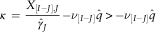$$\kappa \,=\,{{X_{{[I{\minus}J],J}} } \over {\hat{\gamma }_{J} }}{\minus}\nu _{{[I{\minus}J]}} \hat{q}\,\gt\, {\minus}\nu _{{[I{\minus}J]}} \hat{q}$$ ensures that $$\mathop{\sum}\nolimits_{j\,=\,0}^J \hat{\gamma }_{j} \,=\,1$$ . We insert the estimates $$\hat{\gamma }_{j} $$ in the ML equation for q and obtain

(2.19)

$$\hat{q}={{\mathop{\sum}\nolimits_{i\,=\,0}^I {C_{{i,\iota (i)}} } } \over {\mathop{\sum}\nolimits_{i\,=\,0}^I {\nu _{i} } \mathop{\sum}\nolimits_{j\,=\,0}^{\iota (i)} {{{X_{{[I{\minus}j],j}} } \over {\nu _{{[I{\minus}j]}} \hat{q}{\plus}\kappa }}} }}.$$

It follows that

$$\eqalignno{ \mathop{\sum}\limits_{\scriptstyle i{\plus}j\leq I, \hfill \atop \scriptstyle j\leq J \hfill} {X_{{i,j}} } & \,=\,\mathop{\sum}\limits_{i\,=\,0}^I {C_{{i,\iota (i)}} } \mathop{=}\limits^{{(2.19)}} \hat{q}\mathop{\sum}\limits_{\scriptstyle i{\plus}j\leq I, \hfill \atop \scriptstyle j\leq J \hfill} {\nu _{i} {{X_{{[I{\minus}j],j}} } \over {\nu _{{[I{\minus}j]}} \hat{q}{\plus}\kappa }}} \cr &\,=\, \hat{q}\mathop{\sum}\limits_{j\,=\,0}^J {\nu _{{[I{\minus}j]}} {{X_{{[I{\minus}j],j}} } \over {\nu _{{[I{\minus}j]}} \hat{q}{\plus}\kappa }}} ,$$

and hence

$$0=\mathop{\sum}\limits_{j\,=\,0}^J {X_{{[I{\minus}j],j}} } \left( {1{\minus}{{\hat{q}\nu _{{[I{\minus}j]}} } \over {\nu _{{[I{\minus}j]}} \hat{q}{\plus}\kappa }}} \right)=\mathop{\sum}\limits_{j\,=\,0}^J {X_{{[I{\minus}j],j}} {\kappa \over {\nu _{{[I{\minus}j]}} \hat{q}{\plus}\kappa }}} \,=\,\kappa \mathop{\sum}\limits_{j\,=\,0}^J {\hat{\gamma }_{j} } \,=\,\kappa .$$

From κ=0 and the constraint $$\mathop{\sum}\nolimits_{j\,=\,0}^J \hat{\gamma }_{j} \,=\,1$$ it follows with (2.18) that

$$\hat{q}=\mathop{\sum}\limits_{j\,=\,0}^J {{{X_{{[I{\minus}j],j}} } \over {\nu _{{[I{\minus}j]}} }}} ,$$

and from (2.6) we know that $$\hat{q}$$ also satisfies the ML equation (2.17). We conclude that the ML estimates for q and for the γ _j’s under Model Assumptions 2.5 are given by

$$\hat{\gamma }_{j} \,=\,{{{{X_{{[I{\minus}j],j}} } \over {\nu _{{[I{\minus}j]}} }}} \over {\mathop{\sum}\nolimits_{l=0}^J {{{X_{{[I{\minus}l],l}} } \over {\nu _{{[I{\minus}l]}} }}} }}={{\hat{\gamma }_{j}^{{{\rm raw}}} } \over {\hat{\beta }_{J}^{{{\rm raw}}} }},\quad \quad \hat{q}={{\mathop{\sum}\nolimits_{i\,=\,0}^I {C_{{i,\iota (i)}} } } \over {\mathop{\sum}\nolimits_{i\,=\,0}^I {\nu _{i} \hat{\beta }_{{\iota (i)}} } }}=\mathop{\sum}\limits_{l=0}^J {{{X_{{[I{\minus}l],l}} } \over {\nu _{{[I{\minus}l]}} }}} \,=\,\hat{\beta }_{J}^{{{\rm raw}}} ,$$

as in (2.1) and (2.7), which proves the claim.

□

As the parameter estimates are as in (2.1) and (2.7), we can use Estimate 2.3 for the estimation of the conditional MSEP, we just need to replace the estimates for qσ _j², 0≤j≤J, by some estimates for ϕqγ _j. As in Wüthrich & Merz (Reference Wüthrich and Merz2008) we suggest to estimate ϕ with the help of Pearson residuals:

(2.20)

$$\hat{\phi }={1 \over {\,\mid{\cal D}_{I} \mid{\minus}\,(J{\plus}1)}}\mathop{\sum}\limits_{\scriptstyle i{\plus}j\leq I \hfill \atop \scriptstyle j\leq J \hfill} {{{(X_{{i,j}} {\minus}\nu _{i} \hat{\gamma }_{j}^{{{\rm raw}}} )^{2} } \over {\nu _{i} \hat{\gamma }_{j}^{{{\rm raw}}} }}}, $$

where $$\mid{\cal D}_{I} \mid$$ denotes the number of observations in $${\cal D}_{I} $$ . Replacing the estimates $$\widehat{{q\sigma ^{2} }}_{j} $$ by $$\hat{\phi }\hat{\gamma }_{j}^{{{\rm raw}}} $$ in Estimate 2.3 we obtain the following estimators:

Estimate 2.7 (MSEP, ODP model) Under Model Assumptions 2.5 the conditional MSEP of the CC predictor $$\hat{C}_{{i,J}}^{{{\rm CC}}} $$ given in (2.9) is estimated by

$$\widehat{{{\rm MSEP}}}_{{C_{{i,J}} \,\mid\,{\cal D}_{I} }} \left( {\hat{C}_{{i,J}}^{{{\rm CC}}} } \right)=\widehat{{{\rm PV}}}_{i} {\plus}\widehat{{{\rm PEE}}}_{i} \,=\,\hat{\phi }\hat{R}_{i}^{{{\rm CC}}} {\plus}\nu _{i}^{2} \hat{\phi }\mathop{\sum}\limits_{j\,=\,I{\minus}i{\plus}1}^J {{{X_{{[I{\minus}j],j}} } \over {\left( {\nu _{{[I{\minus}j]}} } \right)^{2} }}} ,$$

where $$\hat{\phi }$$ and $$\hat{R}_{i}^{{{\rm CC}}} $$ are given in (2.20) and (2.8). For aggregated accident years the corresponding conditional MSEP is estimated by

$$\eqalignno{ & \widehat{{{\rm MSEP}}}_{{\mathop{\sum}\nolimits_{i\,=\,I{\minus}J{\plus}1}^I {C_{{i,J}} \,\mid\,{\cal D}_{I} } }} \left( {\mathop{\sum}\limits_{i\,=\,I{\minus}J{\plus}1}^I \hat{C}_{{i,J}}^{{{\rm CC}}} } \right)=\mathop{\sum}\limits_{i\,=\,I{\minus}J{\plus}1}^I {\widehat{{{\rm MSEP}}}_{{C_{{i,J}} \,\mid\,{\cal D}_{I} }} \left( {\hat{C}_{{i,J}}^{{{\rm CC}}} } \right)} {\plus}2\mathop{\sum}\limits_{I{\minus}J{\plus}1\leq i\lt k\leq I} {\widehat{{{\rm PEE}}}_{{i,k}} } \cr & \,=\,\mathop{\sum}\limits_{i\,=\,I{\minus}J{\plus}1}^I {\widehat{{{\rm MSEP}}}_{{C_{{i,J}} \,\mid\,{\cal D}_{I} }} \left( {\hat{C}_{{i,J}}^{{{\rm CC}}} } \right)} {\plus}2\mathop{\sum}\limits_{I{\minus}J{\plus}1\leq i\lt k\leq I} {\nu _{i} \nu _{k} \hat{\phi }} \mathop{\sum}\limits_{j\,=\,I{\minus}i{\plus}1}^J {{{X_{{[I{\minus}j],j}} } \over {\left( {\nu _{{[I{\minus}j]}} } \right)^{2} }}} .$$

Analogously an estimator for the uncertainty in the one-year CDR is obtained from Estimate 2.4 by replacing $$\widehat{{q\sigma ^{2} }}_{j} $$ by $$\hat{\phi }\hat{\gamma }_{j}^{{{\rm raw}}} $$ , with $$\hat{\phi }$$ given in (2.20).

Remark 2.8

∙ Under Model Assumptions 2.5, if μ _i=ν _iq, 0≤i≤I, are considered as unknown parameters and if the μ _i’s and γ _j’s are both estimated by ML estimation then it is well-known that the resulting development pattern is the CL development pattern (see e.g. Mack, Reference Mack1991; Renshaw & Verrall, Reference Renshaw and Verrall1998). The result goes back to Hachemeister & Stanard (Reference Hachemeister and Stanard1975). For the estimation of the correlations in the CL development pattern one can therefore use the Fisher information matrix. This approach is also used by Alai et al. (Reference Alai, Merz and Wüthrich2010) to derive an estimate for the conditional MSEP in the BF method in the case where the CL development pattern is used. However, in the CC method the premiums are assumed to be known and hence ignoring this information for the estimation of the development pattern is not consistent with the CC assumptions and thus we do not consider this case in more detail.
∙ Taylor (Reference Taylor2002) remarks that the assumption of a constant dispersion parameter is often not realistic in practice. In Model Assumptions 2.5 the assumption of a constant dispersion parameter ϕ can be replaced by using a different dispersion parameter ϕ _j for each development year. The derivation of the ML estimates in this case is completely analogous and leads to the same estimates for the development pattern and the loss ratio. Further, the estimator (2.10) for qσ _j² gives in this case an estimator for qϕ _jγ _j. Therefore, if we use (2.10) for the estimation of the variance parameters qϕ _jγ _j, we obtain the estimators given in Estimates 2.3 and 2.4 for the conditional MSEPs. Hence, in this case we have the same formulas as in the distribution-free CC model 2.1.

3. Example

To illustrate the results, we apply the method to a data set from Wüthrich & Merz (Reference Wüthrich and Merz2008), which is given in Appendix B. As explained below Remark 1.1, in a company premiums should be adjusted based on the information from the budgeting and planning process. As we do not have information from the budgeting and planning process we assume that the earned premiums given in Appendix B can be used as on-level premiums.

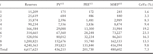
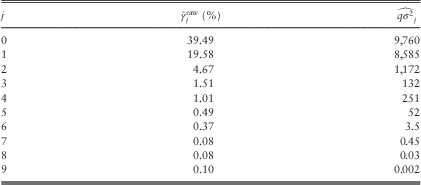
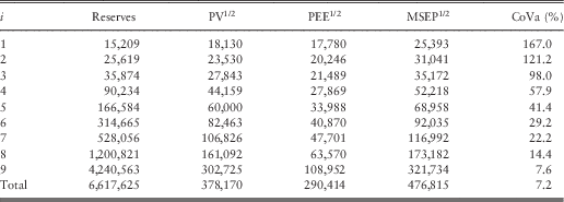
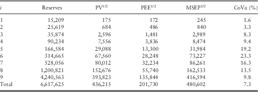
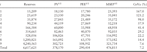
We calculate the reserves, process standard deviation, parameter estimation error and conditional MSEP for the CC model 2.1 and for the ODP model 2.5. Results from the CC model 2.1 are summarised in Table 2. The corresponding parameter estimates are given in Table 3 and the loss ratio estimate is given by $$\hat{q}=\hat{\beta }_{J}^{{{\rm raw}}} \,=\,0.674$$ . The coefficient of variation of a reserve estimate $$\hat{R}_{i} $$ is estimated as

$$\widehat{{{\rm CoVa}}}\left( {\hat{R}_{i} } \right)={{\sqrt {\widehat{{{\rm MSEP}}}_{{R_{i} \,\mid\,{\cal D}_{I} }} \left( {\hat{R}_{i} } \right)} } \over {\hat{R}_{i} }}={{\sqrt {\widehat{{{\rm MSEP}}}_{{C_{{i,J}} \,\mid\,{\cal D}_{I} }} \left( {\hat{C}_{{i,J}} } \right)} } \over {\hat{R}_{i} }}.$$

Table 2

Results CC model 2.1: reserves, process standard deviation (PV^1/2), parameter estimation error (PEE), conditional MSEP and coefficient of variation (CoVa) according to Estimate 2.3.

Table 3

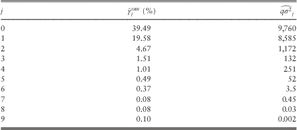
CC model 2.1: parameter estimates (2.2) and (2.10).

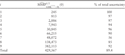
For the CC model 2.1 we also calculate the uncertainty in the CDR given by Estimate 2.4 and we compare these numbers with the conditional MSEP of the ultimate claim (see Estimate 2.3). The results are given in Table 4. Note that

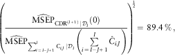$$\left( {{{\widehat{{{\rm MSEP}}}_{{{\rm CDR}^{{(I{\plus}1)}} \,\mid\,{\cal D}_{I} }} (0)} \over {\widehat{{{\rm MSEP}}}_{{\mathop{\sum}\nolimits_{i\,=\,I{\minus}J{\plus}1}^I {C_{{i,J}} \,\mid\,{\cal D}_{I} } }} \left( {\mathop{\sum}\limits_{i\,=\,I{\minus}J{\plus}1}^I {\hat{C}_{{i,J}} } } \right)}}} \right)^{{\!\!{1 \over 2}}} \,=\,89.4\,\%\,,$$

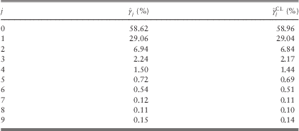
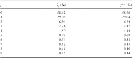
which means that most of the uncertainty in the prediction of the ultimate claim amount is contained in the next accounting year. As stated in Merz & Wüthrich (Reference Merz and Wüthrich2008), this is to be expected for a triangle with short-tailed development. In the claims triangle of our example the development is very short. Most of the claims evolve in the first two development years. This can be observed when considering the normalised development pattern $$\hat{\gamma }_{j} $$ given in Table 5.

Table 4

CC model 2.1: uncertainty in the CDR according to Estimate 2.4 and $$\widehat{{{\rm MSEP}}}_{{{\rm CDR}_{i}^{{(I{\plus}1)}} \,\mid\,{\cal D}_{I} }}^{{1/2}} (0)/\widehat{{{\rm MSEP}}}_{{C_{{i,J}} \,\mid\,{\cal D}_{I} }}^{{1/2}} \left( {\hat{C}_{{i,J}} } \right)$$ for comparison with Estimate 2.3.

Table 5

Normalised development pattern given in (2.1) and CL development pattern.

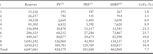
The results obtained from the ODP model 2.5 are given in Table 6. As shown in section 2.2, the reserves and development pattern are the same as in the CC model 2.1. In the ODP model 2.5 we have a constant dispersion parameter ϕ for all development years. The estimates $$\hat{\phi }\hat{\gamma }_{j}^{{{\rm raw}}} $$ for the variance parameters ϕqγ _j should be compared with the corresponding estimates $$\widehat{{q\sigma ^{2} }}_{j} $$ for qσ _j² in the CC model 2.1 (see Tables 3 and 7). As $$\hat{\phi }\hat{\gamma }_{j}^{{{\rm raw}}} \gt \gt \widehat{{q\sigma ^{2} }}_{j} $$ for late development years (see Tables 3 and 7), the process standard deviation and the parameter estimation error in early accident years are much higher in this model compared with the CC model 2.1 (see Tables 2 and 6). However, for the total over all accident years the process standard deviations in the CC model 2.1 (Table 2) are higher than in the ODP model 2.5 (Table 6). As stated in Remark 2.8, the assumption of a constant dispersion parameter is often not appropriate. With the estimates $$\widehat{{q\sigma ^{2} }}_{j} $$ given in (2.10) we define

(3.1)

$$\hat{\phi }_{j} \,=\,{{\widehat{{q\sigma ^{2} }}_{j} } \over {\hat{\gamma }_{j}^{{{\rm raw}}} }},\quad j=0,\ldots,\,J.$$

Note that $$\hat{\phi }_{j} $$ gives an estimate for a dispersion parameter ϕ _j that varies between development years. In our example these dispersion parameters are given in Table 8. The estimate $$\hat{\phi }$$ of the dispersion parameter in the ODP model 2.5 is given by $$\hat{\phi }=21,611$$ (see (2.20)). The variability of the estimates $$\hat{\phi }_{j} $$ given in Table 8 also suggests that the assumption of a constant dispersion parameter is too restrictive.

Table 6

Results ODP model 2.5: reserves, process standard deviation (PV^1/2), parameter estimation error (PEE), conditional MSEP and coefficient of variation (CoVa) according to Estimate 2.7.

Table 7

ODP model 2.5: parameter estimates (2.2) and $$\hat{\phi }$$ as in (2.20).

Table 8

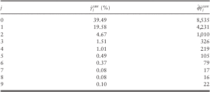
Parameter estimates (3.1) for comparison with $$\hat{\phi }=21,611$$ calculated from (2.20).

For comparison we further give the results obtained with Mack’s CL method (Mack, Reference Mack1993) in Table 9. These results can be found in Wüthrich & Merz (Reference Wüthrich and Merz2008). In Table 5 we compare the CL development pattern to the normalised development pattern given in (2.1). In this example the development patterns are very similar.

Table 9

CL results according to Mack (Reference Mack1993).

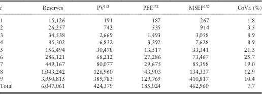
The CL reserves are substantially lower than the CC reserves (see Tables 2 and 9). From the data triangle, we observe that the diagonal values C _i,ι(i) are rather low for accident years 6–8. The relative differences in the reserves of CC and CL are also the highest for these accident years.

As in Wüthrich & Merz (Reference Wüthrich and Merz2008) we plot the individual loss ratios $$C_{{i,\iota (i)}} /(\nu _{i} \hat{\beta }_{{\iota (i)}} )$$ and compare it to the estimated loss ratio $$\hat{q}=0.674$$ (see Figure 1). The picture also shows that the diagonal claims C _i,ι(i) in accident years 7 and 8 are rather low. On the other hand, it is possible that the premium level was increased in these accident years. In a company, information from the budgeting and planning process should be used to adjust the premiums in this case. The decision whether one rather relies on the given diagonal values (by using CL) or whether one trusts the premium information more (by using CC), needs to be based on further information on the data and the quality of the on-level premiums.

Figure 1

Individual loss ratios $${{C_{{i,\iota (i)}} } \over {\nu _{i} \hat{\beta }_{{\iota (i)}} }}$$ and $$\hat{q}=0.674$$ .

4. Conclusion

In this paper we studied the CC method in a stochastic framework. We derive parameter estimates for the development pattern and the loss ratio within the considered stochastic model. The resulting estimates allow to rewrite the CC reserve in a simple form as given in (2.8). Moreover, we derive closed formulas for the conditional MSEP of the ultimate claim as well as for the uncertainties in the one-year CDR. Although the CC method is well established in practice, such formulas cannot be found in current literature (see Dal Moro & Lo, Reference Dal Moro and Lo2014). We further remark that most contributions on the CDR in current literature are in the context of the CL method.

In this paper the relations between the ultimate uncertainties and the uncertainties on a one-year horizon are highlighted, too. In the numerical example it is observed that most of the uncertainty lies in the next accounting year. Such observations are typical for short-tailed lines of business (see Merz & Wüthrich, Reference Merz and Wüthrich2008).

4.1. Limitations and possible extensions

In our stochastic model we have assumed that on-level premiums are known. In practice, such on-level premiums are not always available, and the calculation of on-level premiums can be afflicted with uncertainties. As an alternative to on-level premiums, Bühlmann & Straub (Reference Bühlmann and Straub1983) also allow for varying loss ratio estimates given by

$$\hat{q}_{i} \,=\,{{\mathop{\sum}\nolimits_{i\in S_{i} } {C_{{i,\iota (i)}} } } \over {\mathop{\sum}\nolimits_{i\in S_{i} } {\nu _{i} \hat{\beta }_{{\iota (i)}} } }},$$

where the set S _i⊂{0,1, … ,I} needs to be chosen in such a way that the years in S _i are comparable with accident year i in terms of the expected loss ratio. This means that only the premiums v _k, $$k\in S_{i} $$ , need to be adjusted to the same level. However, if non-constant loss ratios are used, then the estimation of the development pattern and the prediction uncertainties needs to be adjusted. The simple representation of the CC reserves given in (2.8) does then no longer hold. Such adjustments and a corresponding stochastic model could be addressed in future research.

Further, we showed in Remark 2.2 how an externally given tail development can be incorporated in the estimation of the reserves. Future research could investigate how such tail development estimators can be obtained and how the incorporation of such tail developments affects prediction uncertainties.

Acknowledgements

The author would like to thank Alois Gisler, Mario V. Wüthrich and two anonymous referees for valuable comments that helped to improve an earlier version of this paper.

Appendix A

Derivations of the estimators

Derivation of Estimate 2.3

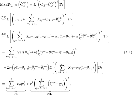
For the conditional MSEP of accident year i≥I−J we have

(A.1)

$$\eqalign{ & {\rm MSEP}_{{C_{{i,J}} \,\mid\,{\cal D}_{I} }} \left( {\hat{C}_{{i,J}}^{{{\rm CC}}} } \right)=E\left[ {\left. {\left( {C_{{i,J}} {\minus}\hat{C}_{{i,J}}^{{{\rm CC}}} } \right)^{2} } \right|{\cal D}_{I} } \right] \cr & \mathop{=}\limits^{{(2.9)}} E\left[ {\left. {\left( {C_{{i,I{\minus}i}} {\plus}\mathop{\sum}\limits_{j\,=\,I{\minus}i{\plus}1}^J {X_{{i,j}} {\minus}C_{{i,I{\minus}i}} {\minus}\hat{R}_{{i,J}}^{{{\rm CC}}} } } \right)^{2} } \right|{\cal D}_{I} } \right] \cr & \mathop{=}\limits^{{(2.8)}} E\left[ {\left. {\left( {\mathop{\sum}\limits_{j\,=\,I{\minus}i{\plus}1}^J {X_{{i,j}} {\minus}\nu _{i} q(1{\minus}\beta _{{I{\minus}i}} ){\plus}\nu _{i} q(1{\minus}\beta _{{I{\minus}i}} ){\minus}\nu _{i} \left( {\hat{\beta }_{J}^{{{\rm raw}}} {\minus}\hat{\beta }_{{I{\minus}i}}^{{{\rm raw}}} } \right)} } \right)^{2} } \right|{\cal D}_{I} } \right] \cr & \;=\mathop{\sum}\limits_{j\,=\,I{\minus}i{\plus}1}^J {{\rm Var}(X_{{i,j}} )} {\plus}\nu _{i}^{2} \left( {\hat{\beta }_{J}^{{{\rm raw}}} {\minus}\hat{\beta }_{{I{\minus}i}}^{{{\rm raw}}} {\minus}q(1{\minus}\beta _{{I{\minus}i}} )} \right)^{2} {(\rm A.1)}\cr & \quad {\plus}2\nu _{i} \left( {q(1{\minus}\beta _{{I{\minus}i}} ){\minus}\hat{\beta }_{J}^{{{\rm raw}}} {\minus}\hat{\beta }_{{I{\minus}i}}^{{{\rm raw}}} } \right)E\left[ {\left. {\left( {\mathop{\sum}\limits_{j\,=\,I{\minus}i{\plus}1}^J {X_{{i,j}} {\minus}\nu _{i} q(1{\minus}\beta _{{I{\minus}i}} )} } \right)} \right|{\cal D}_{I} } \right] \cr & \;=\mathop{\underbrace{{\mathop{\sum}\limits_{j\,=\,I{\minus}i{\plus}1}^J {\nu _{i} q\sigma _{j}^{2} } }}}\limits_{{\rm PV}_{i} }{\plus}\mathop{\underbrace{{\nu _{i}^{2} \left( {\mathop{\sum}\limits_{j\,=\,I{\minus}i{\plus}1}^J {\left( {\hat{\gamma }_{j}^{{{\rm raw}}} {\minus}q\gamma _{j} } \right)} } \right)^{2} }}}\limits_{{\rm PEE}_{i} }, $$

where the mixed term in the second line of equation (A.1) vanishes owing to the independence between (X _i,j)_{j=I−i+1, … ,J} and $${\cal D}_{I} $$ . We estimate the process variance PV_i by inserting the parameter estimates given in (2.10):

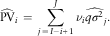$$\widehat{{{\rm PV}}}_{i} \,=\,\mathop{\sum}\limits_{j\,=\,I{\minus}i{\plus}1}^J {\nu _{i} \widehat{{q\sigma ^{2} }}_{j} } .$$

For the estimation of the parameter estimation error of accident year i we observe that $$\hat{\gamma }_{j}^{{{\rm raw}}} $$ is an unbiased estimator for qγ _j (this follows from (2.2)). We approximate parameter estimation error by taking the average overall possible observations $${\cal D}_{I} $$ , that is, we consider the expected value

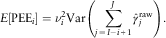$$E[{\rm PEE}_{i} ]=\nu _{i}^{2} {\rm Var}\left( {\mathop{\sum}\limits_{j\,=\,I{\minus}i{\plus}1}^J {\hat{\gamma }_{j}^{{{\rm raw}}} } } \right).$$

Further, $$\hat{\gamma }_{j}^{{{\rm raw}}} $$ depends only on the data from development year j and therefore the $$(\hat{\gamma }_{j}^{{{\rm raw}}} )_{{j\,=\,0,\ldots,\,J}} $$ are independent. Moreover, we have

(A.2)

$$\eqalignno{ {\rm Var}\left( {\hat{\gamma }_{j}^{{{\rm raw}}} } \right)= \,& {\rm Var}\left( {{{\mathop{\sum}\nolimits_{l=0}^{I{\minus}j} {X_{{l,j}} } } \over {\nu _{{[I{\minus}j]}} }}} \right)={1 \over {\left( {\nu _{{[I{\minus}j]}} } \right)^{2} }}\mathop{\sum}\limits_{l=0}^{I{\minus}j} {{\rm Var}(X_{{l,j}} )} \cr \,=\, & {1 \over {\left( {\nu _{{[I{\minus}j]}} } \right)^{2} }}\mathop{\sum}\limits_{l=0}^{I{\minus}j} {\nu _{l} q\sigma _{j}^{2} } \,=\,{{q\sigma _{j}^{2} } \over {\nu _{{[I{\minus}j]}} }} .$$

We therefore obtain

$$\eqalignno{ E[{\rm PEE}_{i} ]=\, & \nu _{i}^{2} {\rm Var}\left( {\mathop{\sum}\limits_{j\,=\,I{\minus}i{\plus}1}^J {\hat{\gamma }_{j}^{{{\rm raw}}} } } \right)=\nu _{i}^{2} \mathop{\sum}\limits_{j\,=\,I{\minus}i{\plus}1}^J {{\rm Var}\left( {\hat{\gamma }_{j}^{{{\rm raw}}} } \right)} \,=\, \nu _{i}^{2} \mathop{\sum}\limits_{j\,=\,I{\minus}i{\plus}1}^J {{{q\sigma _{j}^{2} } \over {\nu _{{[I{\minus}j]}} }}} .$$

Hence we estimate the parameter estimation error by

$$\widehat{{{\rm PEE}}}_{i} \,=\,\nu _{i}^{2} \mathop{\sum}\limits_{j\,=\,I{\minus}i{\plus}1}^J {{{\widehat{{q\sigma ^{2} }}_{j} } \over {\nu _{{[I{\minus}j]}} }}} ,$$

which yields the estimator $$\widehat{{{\rm MSEP}}}_{{C_{{i,J}} \,\mid\,{\cal D}_{I} }} \left( {\hat{C}_{{i,J}}^{{{\rm CC}}} } \right)$$ given in Estimate 2.3.

Next we consider the conditional MSEP of aggregated accident years given by

$$\eqalignno{ & {\rm MSEP}_{{\mathop{\sum}\nolimits_{i\,=\,I{\minus}J{\plus}1}^I {C_{{i,J}} \,\mid\,{\cal D}_{I} } }} \left( {\mathop{\sum}\limits_{i\,=\,I{\minus}J{\plus}1}^I {\hat{C}_{{i,J}}^{{{\rm CC}}} } } \right)=E\left[ {\left. {\left( {\mathop{\sum}\limits_{i\,=\,I{\minus}J{\plus}1}^I {\left( {C_{{i,J}} {\minus}\hat{C}_{{i,J}}^{{{\rm CC}}} } \right)} } \right)^{2} } \right|{\cal D}_{I} } \right] \cr & \,=\,\mathop{\sum}\limits_{i\,=\,I{\minus}J{\plus}1}^I {{\rm MSEP}_{{C_{{i,J}} \,\mid\,{\cal D}_{I} }} (\hat{C}_{{i,J}}^{{{\rm CC}}} )} {\plus}2\mathop{\sum}\limits_{i\,\lt \,k} {E\left[ {\left. {\left( {C_{{i,J}} {\minus}\hat{C}_{{i,J}}^{{{\rm CC}}} } \right)\left( {C_{{k,J}} {\minus}\hat{C}_{{k,J}}^{{{\rm CC}}} } \right)} \right|{\cal D}_{I} } \right]} .$$

As in the case of a single accident year, we use (2.8) and (2.9) to rewrite

$$C_{{i,J}} {\minus}\hat{C}_{{i,J}}^{{{\rm CC}}} \,=\,\mathop{\sum}\limits_{j\,=\,I{\minus}i{\plus}1}^J {X_{{i,j}} } {\minus}\nu _{i} \left( {\hat{\beta }_{J}^{{{\rm raw}}} {\minus}\hat{\beta }_{{I{\minus}i}}^{{{\rm raw}}} } \right).$$

For the mixed terms $$E\left[ {\left. {\left( {C_{{i,J}} {\minus}\hat{C}_{{i,J}}^{{{\rm CC}}} } \right)\left( {C_{{k,J}} {\minus}\hat{C}_{{k,J}}^{{{\rm CC}}} } \right)} \right|{\cal D}_{I} } \right]$$ , i<k, we then obtain

$$\eqalignno{ & E\left[ {\left. {\left( {C_{{i,J}} {\minus}\hat{C}_{{i,J}}^{{{\rm CC}}} } \right)\left( {C_{{k,J}} {\minus}\hat{C}_{{k,J}}^{{{\rm CC}}} } \right)} \right|{\cal D}_{I} } \right] \cr =\, E\left[ {\left. {\left( {\mathop{\sum}\limits_{j\,=\,I{\minus}i{\plus}1}^J {X_{{i,j}} } {\minus}\nu _{i} \left( {\hat{\beta }_{J}^{{{\rm raw}}} {\minus}\hat{\beta }_{{I{\minus}i}}^{{{\rm raw}}} } \right)} \right)\left( {\mathop{\sum}\limits_{j\,=\,I{\minus}k{\plus}1}^J {X_{{k,j}} } {\minus}\nu _{k} \left( {\hat{\beta }_{J}^{{{\rm raw}}} {\minus}\hat{\beta }_{{I{\minus}k}}^{{{\rm raw}}} } \right)} \right)} \right|{\cal D}_{I} } \right] \cr =\, E\left[ {\left. {\left( {\mathop{\sum}\limits_{j\,=\,I{\minus}i{\plus}1}^J {X_{{i,j}} } } \right)\left( {\mathop{\sum}\limits_{j\,=\,I{\minus}k{\plus}1}^J {X_{{k,j}} } } \right)} \right|{\cal D}_{I} } \right]{\minus}E\left[ {\left. {\mathop{\sum}\limits_{j\,=\,I{\minus}i{\plus}1}^J {X_{{i,j}} } } \right|{\cal D}_{I} } \right]\nu _{k} \left( {\hat{\beta }_{J}^{{{\rm raw}}} {\minus}\hat{\beta }_{{I{\minus}k}}^{{{\rm raw}}} } \right) \cr \quad \ {\minus}\,\nu _{i} \left( {\hat{\beta }_{J}^{{{\rm raw}}} {\minus}\hat{\beta }_{{I{\minus}i}}^{{{\rm raw}}} } \right)E\left[ {\left. {\mathop{\sum}\limits_{j\,=\,I{\minus}k{\plus}1}^J {X_{{k,j}} } } \right|{\cal D}_{I} } \right]{\plus}\nu _{i} \left( {\hat{\beta }_{J}^{{{\rm raw}}} {\minus}\hat{\beta }_{{I{\minus}i}}^{{{\rm raw}}} } \right)\nu _{k} \left( {\hat{\beta }_{J}^{{{\rm raw}}} {\minus}\hat{\beta }_{{I{\minus}k}}^{{{\rm raw}}} } \right) \cr =\,\nu _{i} \nu _{k} q^{2} (1{\minus}\beta _{{I{\minus}i}} )(1{\minus}\beta _{{I{\minus}k}} ){\minus}\nu _{i} q(1{\minus}\beta _{{I{\minus}i}} )\nu _{k} \left( {\hat{\beta }_{J}^{{{\rm raw}}} {\minus}\hat{\beta }_{{I{\minus}k}}^{{{\rm raw}}} } \right) \cr \quad {\minus} \, \nu _{i} \left( {\hat{\beta }_{J}^{{{\rm raw}}} {\minus}\hat{\beta }_{{I{\minus}i}}^{{{\rm raw}}} } \right)\nu _{k} q(1{\minus}\beta _{{I{\minus}k}} ){\plus}\nu _{i} \left( {\hat{\beta }_{J}^{{{\rm raw}}} {\minus}\hat{\beta }_{{I{\minus}i}}^{{{\rm raw}}} } \right)\nu _{k} \left( {\hat{\beta }_{J}^{{{\rm raw}}} {\minus}\hat{\beta }_{{I{\minus}k}}^{{{\rm raw}}} } \right) ,$$

where we used the independence of the incremental claims $$X_{{i,j}} $$ . This expression can be rewritten as follows

$$\eqalignno{ & E\left[ {\left. {\left( {C_{{i,J}} {\minus}\hat{C}_{{i,J}}^{{{\rm CC}}} } \right)\left( {C_{{k,J}} {\minus}\hat{C}_{{k,J}}^{{{\rm CC}}} } \right)} \right|{\cal D}_{I} } \right] \cr \,=\,\nu _{i} \nu _{k} q(1{\minus}\beta _{{I{\minus}i}} )\left( {q(1{\minus}\beta _{{I{\minus}k}} ){\minus}\left( {\hat{\beta }_{J}^{{{\rm raw}}} {\minus}\hat{\beta }_{{I{\minus}k}}^{{{\rm raw}}} } \right)} \right) \cr \quad \ {\minus}\,\nu _{i} \nu _{k} \left( {\hat{\beta }_{J}^{{{\rm raw}}} {\minus}\hat{\beta }_{{I{\minus}i}}^{{{\rm raw}}} } \right)\left( {q(1{\minus}\beta _{{I{\minus}k}} ){\minus}\left( {\hat{\beta }_{J}^{{{\rm raw}}} {\minus}\hat{\beta }_{{I{\minus}k}}^{{{\rm raw}}} } \right)} \right) \cr =\,\nu _{i} \nu _{k} \left( {q(1{\minus}\beta _{{I{\minus}i}} ){\minus}\left( {\hat{\beta }_{J}^{{{\rm raw}}} {\minus}\hat{\beta }_{{I{\minus}i}}^{{{\rm raw}}} } \right)} \right)\left( {q(1{\minus}\beta _{{I{\minus}k}} ){\minus}\left( {\hat{\beta }_{J}^{{{\rm raw}}} {\minus}\hat{\beta }_{{I{\minus}k}}^{{{\rm raw}}} } \right)} \right) .$$

Therefore, we need to estimate for i<k

$$\eqalignno{ {\rm PEE}_{{i,k}} \,=\, & \nu _{i} \nu _{k} \left( {\hat{\beta }_{J}^{{{\rm raw}}} {\minus}\hat{\beta }_{{I{\minus}i}}^{{{\rm raw}}} {\minus}q(1{\minus}\beta _{{I{\minus}i}} )} \right)\left( {\hat{\beta }_{J}^{{{\rm raw}}} {\minus}\hat{\beta }_{{I{\minus}k}}^{{{\rm raw}}} {\minus}q(1{\minus}\beta _{{I{\minus}k}} )} \right) \cr \,=\, & \nu _{i} \nu _{k} \left( {\mathop{\sum}\limits_{j\,=\,I{\minus}i{\plus}1}^J {\left( {\hat{\gamma }_{j}^{{{\rm raw}}} {\minus}q\gamma _{j} } \right)} } \right)\left( {\mathop{\sum}\limits_{l=I{\minus}k{\plus}1}^J {\left( {\hat{\gamma }_{l}^{{{\rm raw}}} {\minus}q\gamma _{l} } \right)} } \right) .$$

We approximate PEE_i,k by its expected value

$$\eqalignno{ E[{\rm PEE}_{{i,k}} ]\,=\, & \nu _{i} \nu _{k} {\rm Cov}\left( {\mathop{\sum}\limits_{j\,=\,I{\minus}i{\plus}1}^J {\hat{\gamma }_{j}^{{{\rm raw}}} } ,\mathop{\sum}\limits_{l=I{\minus}k{\plus}1}^J {\hat{\gamma }_{l}^{{{\rm raw}}} } } \right) \cr \,=\, & \nu _{i} \nu _{k} \mathop{\sum}\limits_{j\,=\,I{\minus}i{\plus}1}^J {{\rm Var}\left( {\hat{\gamma }_{j}^{{{\rm raw}}} } \right)} \cr &\!\!\!\!\!\!\!\mathop{=}\limits^{{({\rm A}.2)}} \nu _{i} \nu _{k} \mathop{\sum}\limits_{j\,=\,I{\minus}i{\plus}1}^J {{{q\sigma _{j}^{2} } \over {\nu _{{[I{\minus}j]}} }}} ,\quad i\,\lt \,k ,$$

and estimate PEE_i,k by

$$\widehat{{{\rm PEE}}}_{{i,k}} \,=\,\nu _{i} \nu _{k} \mathop{\sum}\limits_{j\,=\,I{\minus}i{\plus}1}^J {{{\widehat{{q\sigma ^{2} }}_{j} } \over {\nu _{{[I{\minus}j]}} }}} ,\quad i\,\lt \,k.$$

Therefore we derived the formulas given in Estimate 2.3.□

Derivation of Estimate 2.4:

From (2.14) and (2.15) we obtain for I+1−J≤i≤I

$$\eqalignno{ {\rm CDR}_{i}^{{(I{\plus}1)}} \,&=\,\hat{C}_{{i,J}}^{{(I)}} {\minus}\hat{C}_{{i,J}}^{{(I{\plus}1)}} \cr &\,=\,{\minus}X_{{i,I{\plus}1{\minus}i}} {\plus}\nu _{i} \left( {\hat{\beta }_{J}^{{(I){\rm raw}}} {\minus}\hat{\beta }_{{I{\minus}i}}^{{(I){\rm raw}}} {\minus}\hat{\beta }_{J}^{{(I{\plus}1){\rm raw}}} {\plus}\hat{\beta }_{{I{\plus}1{\minus}i}}^{{(I{\plus}1){\rm raw}}} } \right) \cr & \,=\,{\minus}X_{{i,I{\plus}1{\minus}i}} {\plus}\nu _{i} \left( {\mathop{\sum}\limits_{j\,=\,I{\plus}1{\minus}i}^J {\hat{\gamma }_{j}^{{(I){\rm raw}}} } {\minus}\mathop{\sum}\limits_{j\,=\,I{\plus}2{\minus}i}^J {\hat{\gamma }_{j}^{{(I{\plus}1){\rm raw}}} } } \right) .$$

Note that

$$\eqalignno{ \hat{\gamma }_{j}^{{(I{\plus}1){\rm raw}}} \mathop{=}\limits^{{(2.16)}} {{X_{{[I{\plus}1{\minus}j],j}} } \over {\nu _{{[I{\plus}1{\minus}j]}} }}=\nu _{{[I{\minus}j]}} {{X_{{[I{\minus}j],j}} {\plus}X_{{I{\plus}1{\minus}j,j}} } \over {\nu _{{[I{\minus}j]}} \nu _{{[I{\plus}1{\minus}j]}} }} \cr =\,\hat{\gamma }_{j}^{{(I){\rm raw}}} {{\nu _{{[I{\minus}j]}} } \over {\nu _{{[I{\plus}1{\minus}j]}} }}{\plus}{{X_{{I{\plus}1{\minus}j}} } \over {\nu _{{[I{\plus}1{\minus}j]}} }} .$$

Hence we obtain for I+1−J≤i≤I

(A.3)

$$\eqalignno{ {\rm CDR}_{i}^{{(I{\plus}1)}} =\,{\minus}X_{{i,I{\plus}1{\minus}i}} {\plus}\nu _{i} \left( {\hat{\gamma }_{{I{\plus}1{\minus}i}}^{{(I){\rm raw}}} {\plus}\mathop{\sum}\limits_{j\,=\,I{\plus}2{\minus}i}^J \left( {\hat{\gamma }_{j}^{{(I){\rm raw}}} \left( {1{\minus}{{\nu _{{[I{\minus}j]}} } \over {\nu _{{[I{\plus}1{\minus}j]}} }}} \right){\minus}{{X_{{I{\plus}1{\minus}j,j}} } \over {\nu _{{[I{\plus}1{\minus}j]}} }}} \right)} \right) \cr =\,\nu _{i} q\gamma _{{I{\plus}1{\minus}i}} {\minus}X_{{i,I{\plus}1{\minus}i}} {\plus}\nu _{i} \left( {\hat{\gamma }_{{I{\plus}1{\minus}i}}^{{(I){\rm raw}}} {\minus}q\gamma _{{I{\plus}1{\minus}i}} } \right) \cr \qquad & \qquad{\plus}\nu _{i} \mathop{\sum}\limits_{j\,=\,I{\plus}2{\minus}i}^J \left( {\hat{\gamma }_{j}^{{(I){\rm raw}}} {{\nu _{{I{\plus}1{\minus}j}} } \over {\nu _{{[I{\plus}1{\minus}j]}} }}{\minus}{{X_{{I{\plus}1{\minus}j,j}} } \over {\nu _{{[I{\plus}1{\minus}j]}} }}} \right) \cr =\,\nu _{i} q\gamma _{{I{\plus}1{\minus}i}} {\minus}X_{{i,I{\plus}1{\minus}i}} {\plus}\nu _{i} \left( {\hat{\gamma }_{{I{\plus}1{\minus}i}}^{{(I){\rm raw}}} {\minus}q\gamma _{{I{\plus}1{\minus}i}} } \right) \cr \quad & \qquad{\plus}\nu _{i} \mathop{\sum}\limits_{j\,=\,I{\plus}2{\minus}i}^J \left( {\left( {\hat{\gamma }_{j}^{{(I){\rm raw}}} {\minus}q\gamma _{j} } \right){{\nu _{{I{\plus}1{\minus}j}} } \over {\nu _{{[I{\plus}1{\minus}j]}} }}{\minus}{{X_{{I{\plus}1{\minus}j,j}} {\minus}\nu _{{I{\plus}1{\minus}j}} q\gamma _{j} } \over {\nu _{{[I{\plus}1{\minus}j]}} }}} \right) .$$

Therefore we have for the conditional MSEP

(A.4)

$$\eqalignno{ {\rm MSEP}_{{{\rm CDR}_{i}^{{(I{\plus}1)}} \,\mid\,{\cal D}_{I} }} (0) & \,=\,E\left[ {\left. {\left( {{\rm CDR}_{i}^{{(I{\plus}1)}} } \right)^{2} } \right|{\cal D}_{I} } \right] \cr & \,=\,\nu _{i} q\sigma _{{I{\plus}1{\minus}i}}^{2} {\plus}\nu _{i}^{2} \left( {\hat{\gamma }_{{I{\plus}1{\minus}i}}^{{(I){\rm raw}}} {\minus}q\gamma _{{I{\plus}1{\minus}i}} } \right)^{2} \cr \quad & \qquad {\plus}2\nu _{i}^{2} \left( {\hat{\gamma }_{{I{\plus}1{\minus}i}}^{{(I){\rm raw}}} {\minus}q\gamma _{{I{\plus}1{\minus}i}} } \right)\left( {\mathop{\sum}\limits_{j\,=\,I{\plus}2{\minus}i}^J \left( {\hat{\gamma }_{j}^{{(I){\rm raw}}} {\minus}q\gamma _{j} } \right){{\nu _{{I{\plus}1{\minus}j}} } \over {\nu _{{[I{\plus}1{\minus}j]}} }}} \right) $$

(A.5)

$$\quad {\plus}\nu _{i}^{2} E\left[ {\left. {\left( {\mathop{\sum}\limits_{j\,=\,I{\plus}2{\minus}i}^J \left( {\left( {\hat{\gamma }_{j}^{{(I){\rm raw}}} {\minus}q\gamma _{j} } \right){{\nu _{{I{\plus}1{\minus}j}} } \over {\nu _{{[I{\plus}1{\minus}j]}} }}{\minus}{{X_{{I{\plus}1{\minus}j,j}} {\minus}\nu _{{I{\plus}1{\minus}j}} q\gamma _{j} } \over {\nu _{{[I{\plus}1{\minus}j]}} }}} \right)} \right)^{2} } \right|{\cal D}_{I} } \right],$$

where we used that

$$\eqalignno{ 0 & \,=\,\nu _{i} E\left[ {\left. {\left( {\nu _{i} q\gamma _{{I{\plus}1{\minus}i}} {\minus}X_{{i,I{\plus}1{\minus}i}} } \right)\left( {\hat{\gamma }_{{I{\plus}1{\minus}i}}^{{(I){\rm raw}}} {\minus}q\gamma _{{I{\plus}1{\minus}i}} } \right)} \right|{\cal D}_{I} } \right] \cr \quad & \qquad{\plus}\nu _{i} E\left[ {\left. {\left( {\nu _{i} q\gamma _{{I{\plus}1{\minus}i}} {\minus}X_{{i,I{\plus}1{\minus}i}} } \right)\left( {\mathop{\sum}\limits_{j\,=\,I{\plus}2{\minus}i}^J \left( {\left( {\hat{\gamma }_{j}^{{(I){\rm raw}}} {\minus}q\gamma _{j} } \right){{\nu _{{I{\plus}1{\minus}j}} } \over {\nu _{{[I{\plus}1{\minus}j]}} }}} \right)} \right)} \right|{\cal D}_{I} } \right] \cr \quad & \qquad{\minus}\nu _{i} E\left[ {\left. {\left( {\nu _{i} q\gamma _{{I{\plus}1{\minus}i}} {\minus}X_{{i,I{\plus}1{\minus}i}} } \right)\left( {\mathop{\sum}\limits_{j\,=\,I{\plus}2{\minus}i}^J \left( {{{X_{{I{\plus}1{\minus}j,j}} {\minus}\nu _{{I{\plus}1{\minus}j}} q\gamma _{j} } \over {\nu _{{[I{\plus}1{\minus}j]}} }}} \right)} \right)} \right|{\cal D}_{I} } \right] ,$$

due to the independence of $$X_{{i,I{\plus}1{\minus}i}} $$ from $$(X_{{I{\plus}1{\minus}j,j}} )_{{j\,=\,I{\plus}2{\minus}i,\,\ldots\,,J}} $$ and $${\cal D}_{I} $$ . For the conditional expected value given in (A.5) we have

(A.6)

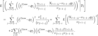$$\eqalignno{ E & \left[ {\left. {\left( {\mathop{\sum}\limits_{j\,=\,I{\plus}2{\minus}i}^J \left( {\left( {\hat{\gamma }_{j}^{{(I){\rm raw}}} {\minus}q\gamma _{j} } \right){{\nu _{{I{\plus}1{\minus}j}} } \over {\nu _{{[I{\plus}1{\minus}j]}} }}{\minus}{{X_{{I{\plus}1{\minus}j,j}} {\minus}\nu _{{I{\plus}1{\minus}j}} q\gamma _{j} } \over {\nu _{{[I{\plus}1{\minus}j]}} }}} \right)} \right)^{2} } \right|{\cal D}_{I} } \right] \cr & \,=\,\mathop{\sum}\limits_{j\,=\,I{\plus}2{\minus}i}^J \left( {\hat{\gamma }_{j}^{{(I){\rm raw}}} {\minus}q\gamma _{j} } \right)^{2} {{\nu _{{I{\plus}1{\minus}j}}^{2} } \over {\left( {\nu _{{[I{\plus}1{\minus}j]}} } \right)^{2} }}{\plus}\mathop{\sum}\limits_{j\,=\,I{\plus}2{\minus}i}^J E\left[ {\left( {{{X_{{I{\plus}1{\minus}j,j}} {\minus}\nu _{{I{\plus}1{\minus}j}} q\gamma _{j} } \over {\nu _{{[I{\plus}1{\minus}j]}} }}} \right)^{2} } \right] \cr \quad & \qquad{\plus}2\mathop{\sum}\limits_{j\,\lt \,k} \left( {\hat{\gamma }_{j}^{{(I){\rm raw}}} {\minus}q\gamma _{j} } \right)\left( {\hat{\gamma }_{k}^{{(I){\rm raw}}} {\minus}q\gamma _{k} } \right){{\nu _{{I{\plus}1{\minus}j}} \nu _{{I{\plus}1{\minus}k}} } \over {\nu _{{[I{\plus}1{\minus}j]}} \nu _{{[I{\plus}1{\minus}k]}} }} .$$

As in the case of the conditional MSEP of the ultimate claim, we approximate the unknown terms by their expected values. Because of the independence of the $$(\hat{\gamma }_{j}^{{{\rm raw}}} )_{{j\,=\,0,\ldots,J}} $$ , the expected values of the terms in line (A.4) and (A.6) are 0. After replacing the unknown parameters by their estimates we get the following estimator

$$\eqalignno{ & \widehat{{{\rm MSEP}}}_{{{\rm CDR}_{i}^{{(I{\plus}1)}} \,\mid\,{\cal D}_{I} }} (0) \cr & \,=\,\nu _{i} \widehat{{q\sigma ^{2} }}_{{I{\plus}1{\minus}i}} {\plus}\nu _{i}^{2} \widehat{{{\rm Var}}}\left( {\hat{\gamma }_{{I{\plus}1{\minus}i}}^{{(I){\rm raw}}} } \right){\plus}\nu _{i}^{2} \mathop{\sum}\limits_{j\,=\,I{\plus}2{\minus}i}^J \left( {\widehat{{{\rm Var}}}\left( {\hat{\gamma }_{j}^{{(I){\rm raw}}} } \right){{\nu _{{I{\plus}1{\minus}j}}^{2} } \over {\left( {\nu _{{[I{\plus}1{\minus}j]}} } \right)^{2} }}{\plus}{{\widehat{{{\rm Var}}}(X_{{I{\plus}1{\minus}j,j}} )} \over {\left( {\nu _{{[I{\plus}1{\minus}j]}} } \right)^{2} }}} \right) ,$$

where the variances $${\rm Var}\left( {\hat{\gamma }_{j}^{{(I){\rm raw}}} } \right)$$ and $${\rm Var}(X_{{I{\plus}1{\minus}j,j}} )$$ are estimated by inserting the parameter estimates for $$q\sigma _{j}^{2} $$ given in (2.10), that is:

$$\widehat{{{\rm Var}}}\left( {\hat{\gamma }_{j}^{{(I){\rm raw}}} } \right)={{\widehat{{q\sigma ^{2} }}_{j} } \over {\nu _{{[I{\minus}j]}} }}\quad {\rm and}\quad \widehat{{{\rm Var}}}(X_{{I{\plus}1{\minus}j,j}} )=\nu _{{I{\plus}1{\minus}j}} \widehat{{q\sigma ^{2} }}_{j} .$$

Therefore we arrive at the estimator

$$\eqalignno{ \widehat{{ {\rm MSEP}}}_{{{\rm CDR}_{i}^{{(I{\plus}1)}} \,\mid\,{\cal D}_{I} }} (0) =\,\nu _{i} \widehat{{q\sigma ^{2} }}_{{I{\plus}1{\minus}i}} {\plus}\nu _{i}^{2} {{\widehat{{q\sigma ^{2} }}_{{I{\plus}1{\minus}i}} } \over {\nu _{{[i{\minus}1]}} }}{\plus}\nu _{i}^{2} \mathop{\sum}\limits_{j\,=\,I{\plus}2{\minus}i}^J {\left( {{{\widehat{{q\sigma ^{2} }}_{j} } \over {\nu _{{[I{\minus}j]}} }}{{\nu _{{I{\plus}1{\minus}j}}^{2} } \over {\left( {\nu _{{[I{\plus}1{\minus}j]}} } \right)^{2} }}{\plus}{{\nu _{{I{\plus}1{\minus}j}} \widehat{{q\sigma ^{2} }}_{j} } \over {\left( {\nu _{{[I{\plus}1{\minus}j]}} } \right)^{2} }}} \right)} \cr & \,=\,\nu _{i} \widehat{{q\sigma ^{2} }}_{{I{\plus}1{\minus}i}} {{\nu _{{[i]}} } \over {\nu _{{[i{\minus}1]}} }}{\plus}\nu _{i}^{2} \mathop{\sum}\limits_{j\,=\,I{\plus}2{\minus}i}^J {\widehat{{q\sigma ^{2} }}_{j} {{\nu _{{I{\plus}1{\minus}j}} } \over {\nu _{{[I{\minus}j]}} \nu _{{[I{\plus}1{\minus}j]}} }}} ,$$

as given in Estimate 2.4.

Similarly, we have for aggregated accident years

$${\rm MSEP}_{{{\rm CDR}^{{(I{\plus}1)}} \,\mid\,{\cal D}_{I} }} (0)=\mathop{\sum}\limits_{i\,=\,I{\minus}J{\plus}1}^I {{\rm MSEP}_{{{\rm CDR}_{i}^{{(I{\plus}1)}} \,\mid\,{\cal D}_{I} }} (0)} {\plus}2\mathop{\sum}\limits_{i\,\lt \,k} {E\left[ {\left. {{\rm CDR}_{i}^{{(I{\plus}1)}} {\rm CDR}_{k}^{{(I{\plus}1)}} } \right|{\cal D}_{I} } \right]}. $$

With the representation of CDR_i^(I+1) given in equation (A.3), it follows that for i<k

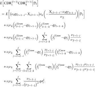$$\eqalignno{ & E\left[ {\left. {{\rm CDR}_{i}^{{(I{\plus}1)}} {\rm CDR}_{k}^{{(I{\plus}1)}} } \right|{\cal D}_{I} } \right] \cr & \,=\,E\left[ {\left. {\left( {\nu _{i} q\gamma _{{I{\plus}1{\minus}i}} {\minus}X_{{i,I{\plus}1{\minus}i}} } \right)\nu _{k} \left( {{\minus}{{X_{{i,I{\plus}1{\minus}i}} {\minus}\nu _{i} q\gamma _{{I{\plus}1{\minus}i}} } \over {\nu _{{[i]}} }}} \right)} \right|{\cal D}_{I} } \right] \cr & \quad {\plus}\nu _{i} \nu _{k} \left( {\hat{\gamma }_{{I{\plus}1{\minus}i}}^{{(I){\rm raw}}} {\minus}q\gamma _{{I{\plus}1{\minus}i}} } \right)\left( {\hat{\gamma }_{{I{\plus}1{\minus}k}}^{{(I){\rm raw}}} {\minus}q\gamma _{{I{\plus}1{\minus}k}} } \right) \cr & \quad {\plus}\nu _{i} \nu _{k} \left( {\hat{\gamma }_{{I{\plus}1{\minus}i}}^{{(I){\rm raw}}} {\minus}q\gamma _{{I{\plus}1{\minus}i}} } \right)\mathop{\sum}\limits_{j\,=\,I{\plus}2{\minus}k}^J {\left( {\hat{\gamma }_{j}^{{(I){\rm raw}}} {\minus}q\gamma _{j} } \right){{\nu _{{I{\plus}1{\minus}j}} } \over {\nu _{{[I{\plus}1{\minus}j]}} }}} \cr & \quad {\plus}\nu _{i} \nu _{k} \mathop{\sum}\limits_{j\,=\,I{\plus}2{\minus}i}^J {\left( {\hat{\gamma }_{j}^{{(I){\rm raw}}} {\minus}q\gamma _{j} } \right){{\nu _{{I{\plus}1{\minus}j}} } \over {\nu _{{[I{\plus}1{\minus}j]}} }}\left( {\hat{\gamma }_{{I{\plus}1{\minus}k}}^{{(I){\rm raw}}} {\minus}q\gamma _{{I{\plus}1{\minus}k}} } \right)} \cr & \quad {\plus}\nu _{i} \nu _{k} \mathop{\sum}\limits_{j\,=\,I{\plus}2{\minus}i}^J {\mathop{\sum}\limits_{l=I{\plus}2{\minus}k}^J {\left( {\hat{\gamma }_{j}^{{(I){\rm raw}}} {\minus}q\gamma _{j} } \right)\left( {\hat{\gamma }_{l}^{{(I){\rm raw}}} {\minus}q\gamma _{l} } \right){{\nu _{{I{\plus}1{\minus}j}} \nu _{{I{\plus}1{\minus}l}} } \over {\nu _{{[I{\plus}1{\minus}j]}} \nu _{{[I{\plus}1{\minus}l]}} }}} } \cr & \quad {\plus}\nu _{i} \nu _{k} \mathop{\sum}\limits_{j\,=\,I{\plus}2{\minus}i}^J {{{\nu _{{I{\plus}1{\minus}j}} } \over {\left( {\nu _{{[I{\plus}1{\minus}j]}} } \right)^{2} }}q\sigma _{j}^{2} } .$$

Further we calculate

$$E\left[ {\left. {\left( {\nu _{i} q\gamma _{{I{\plus}1{\minus}i}} {\minus}X_{{i,I{\plus}1{\minus}i}} } \right)\nu _{k} \left( {{\minus}{{X_{{i,I{\plus}1{\minus}i}} {\minus}\nu _{i} q\gamma _{{I{\plus}1{\minus}i}} } \over {\nu _{{[i]}} }}} \right)} \right|{\cal D}_{I} } \right]=\nu _{k} {{\nu _{i} } \over {\nu _{{[i]}} }}q\sigma _{{I{\plus}1{\minus}i}}^{2} .$$

The mixed term $$E\left[ {\left. {{\rm CDR}_{i}^{{(I{\plus}1)}} {\rm CDR}_{k}^{{(I{\plus}1)}} } \right|{\cal D}_{I} } \right]$$ , i<k, is then approximated by its unconditional expected value which yields

$$\eqalignno{ & \nu _{k} {{\nu _{i} } \over {\nu _{{[i]}} }}q\sigma _{{I{\plus}1{\minus}i}}^{2} {\plus}\nu _{i} \nu _{k} {{\nu _{i} q\sigma _{{I{\plus}1{\minus}i}}^{2} } \over {\nu _{{[i]}} \nu _{{[i{\minus}1]}} }}{\plus}\nu _{i} \nu _{k} \mathop{\sum}\limits_{j\,=\,I{\plus}2{\minus}i}^J {{{q\sigma _{j}^{2} \nu _{{I{\plus}1{\minus}j}}^{2} } \over {\nu _{{[I{\minus}j]}} (\nu _{{[I{\plus}1{\minus}j]}} )^{2} }}{\plus}\nu _{i} \nu _{k} } \mathop{\sum}\limits_{j\,=\,I{\plus}2{\minus}i}^J {{{\nu _{{I{\plus}1{\minus}j}} } \over {\left( {\nu _{{[I{\plus}1{\minus}j]}} } \right)^{2} }}q\sigma _{j}^{2} } \cr & \,=\,\nu _{i} \nu _{k} \left( {{{q\sigma _{{I{\plus}1{\minus}i}}^{2} } \over {\nu _{{[i{\minus}1]}} }}{\plus}\mathop{\sum}\limits_{j\,=\,I{\plus}2{\minus}i}^J {{{q\sigma _{j}^{2} \nu _{{I{\plus}1{\minus}j}} } \over {\nu _{{[I{\minus}j]}} \nu _{{[I{\plus}1{\minus}j]}} }}} } \right) ,$$

where we used the independence of the $$(\hat{\gamma }_{j}^{{{\rm raw}}} )_{{j\,=\,0,\ldots,J}} $$ . After inserting the parameter estimates we arrive at the formula given in Estimate 2.4.□

Appendix B Data

Table B.1

Cumulative payments C _i,j and premiums ν _i.

References

Alai, D.H., Merz, M. & Wüthrich, M.V. (2010). Prediction uncertainty in the Bornhuetter-Ferguson claims reserving method: revisited. Annals of Actuarial Science, 5(1), 7–17.Google Scholar

Bornhuetter, R.L. & Ferguson, R.E. (1972). Proceedings of the Casualty Actuarial Society. The actuary and IBNR. Proc. Cas, LIX, 181–195.Google Scholar

Bühlmann, H., De Felice, M., Gisler, A., Moriconi, F. & Wüthrich, M.V. (2009). Recursive credibility formula for chain ladder factors and the claims development result. ASTIN Bulletin, 39(1), 275–306.Google Scholar

Bühlmann, H. & Straub, E. (1983). Estimation of IBNR Reserves by the Methods Chain Ladder, Cape Cod and Complementary Loss Ratio. International Summer School of the Swiss Association of Actuaries, Leysin, Switzerland.Google Scholar

Dal Moro, E. & Lo, J. (2014). An industry question: the ultimate and one-year reserving uncertainty for different non-life reserving methodologies. ASTIN Bulletin, 44(3), 495–499.CrossRef Google Scholar

England, P.D. & Verrall, R.J. (2002). Stochastic claims reserving in general insurance. British Actuarial Journal, 8(3), 443–518.Google Scholar

FINMA (2006). Technisches Dokument zum Swiss Solvency Test, Version 02/10/2006, technical report, Bundesamt für Privatversicherungen, Bern, Switzerland.Google Scholar

Hachemeister, C. & Stanard, J. (1975). IBNR claims count estimation with static lag functions. ASTIN Colloquium, Portimao, Portugal. September 30 – October 3, 1975.Google Scholar

Mack, T. (1991). A simple parametric model for rating automobile insurance or estimating IBNR claims reserves. ASTIN Bulletin, 21(1), 93–109.Google Scholar

Mack, T. (1993). Distribution-free calculation of the standard error of chain ladder reserve estimates. ASTIN Bulletin, 23(2), 213–225.Google Scholar

Mack, T. (2006). Parameter estimation for Bornhuetter/Ferguson. CAS Forum, (Fall 2006), 141–157.Google Scholar

Mack, T. (2008). The prediction error of Bornhuetter/Ferguson. ASTIN Bulletin, 38(1), 87–103.CrossRef Google Scholar

Merz, M. & Wüthrich, M.V. (2008). Modelling the claims development result for solvency purposes. CAS Forum, (Fall 2008), 542–568.Google Scholar

Renshaw, A.E. & Verrall, R.J. (1998). A stochastic model for the chain ladder method. British Actuarial Journal, 14, 903–923.Google Scholar

Saluz, A., Gisler, A. & Wüthrich, M.V. (2011). Development pattern and prediction error for the stochastic Bornhuetter-Ferguson claims reserving method. ASTIN Bulletin, 41(2), 279–313.Google Scholar

Straub, E. (1988). Non-Life Insurance Mathematics. Springer-Verlag, Association of Swiss Actuaries, Zürich.Google Scholar

Taylor, G.C. (2002). Written discussion on the paper “Stochastic claims reserving in general insurance” by P. D. England and R. J. Verrall. British Actuarial Journal, 8(3), 540–542.Google Scholar

Wüthrich, M.V. & Merz, M. (2008). Stochastic Claims Reserving Methods in Insurance. Wiley, Chichester.Google Scholar

Table 1Claims development triangle.

Table 2Results CC model 2.1: reserves, process standard deviation (PV1/2), parameter estimation error (PEE), conditional MSEP and coefficient of variation (CoVa) according to Estimate 2.3.

Table 3CC model 2.1: parameter estimates (2.2) and (2.10).

Table 4CC model 2.1: uncertainty in the CDR according to Estimate 2.4 and $$\widehat{{{\rm MSEP}}}_{{{\rm CDR}_{i}^{{(I{\plus}1)}} \,\mid\,{\cal D}_{I} }}^{{1/2}} (0)/\widehat{{{\rm MSEP}}}_{{C_{{i,J}} \,\mid\,{\cal D}_{I} }}^{{1/2}} \left( {\hat{C}_{{i,J}} } \right)$$ for comparison with Estimate 2.3.

Table 5Normalised development pattern given in (2.1) and CL development pattern.

Table 6Results ODP model 2.5: reserves, process standard deviation (PV1/2), parameter estimation error (PEE), conditional MSEP and coefficient of variation (CoVa) according to Estimate 2.7.

Table 7ODP model 2.5: parameter estimates (2.2) and $$\hat{\phi }$$ as in (2.20).

Table 8Parameter estimates (3.1) for comparison with $$\hat{\phi }=21,611$$ calculated from (2.20).

Table 9CL results according to Mack (1993).

Figure 1Individual loss ratios $${{C_{{i,\iota (i)}} } \over {\nu _{i} \hat{\beta }_{{\iota (i)}} }}$$ and $$\hat{q}=0.674$$.

Table B.1Cumulative payments Ci,j and premiums νi.

Article contents

Prediction uncertainties in the Cape Cod reserving method

Abstract

Keywords

Information

1. Introduction

1.1. Notation and data structure

1.2. CL method

1.3. CC method

2. Stochastic model for the CC method

2.1. CC method in a distribution-free model

2.1.1. Parameter estimation

2.1.1. Prediction uncertainty

2.1.2. Conditional MSEP of the one-year CDR

2.2. ODP model

3. Example

4. Conclusion

4.1. Limitations and possible extensions

Acknowledgements

Appendix A

Derivations of the estimators

Appendix B Data

References

Save article to Kindle

Save article to Dropbox

Save article to Google Drive

Reply to: Submit a response

Your details

You have entered the maximum number of contributors

Conflicting interests