



1 Introduction
Construction of high order accurate methods for hyperbolic conservation laws
 $$ \begin{align} U_t+f(U)_x=0, \end{align} $$
has attracted the interest of many researchers. One of the main challenges of such research is the development of high order schemes that avoid spurious oscillations and maintain numerical stability, especially in the presence of shocks. Consequently, much effort has been spent to construct spatial discretizations that can preserve certain nonlinear stability properties, such as total variation stability and positivity [Reference Balsara and Shu8, Reference Cockburn and Shu14, Reference Qiu and Shu39, Reference Sweby42]. The most commonly used approach in developing these methods is the methods of lines (MOL). One of the main appealing aspects of this approach is decoupling the spatial and time discretizations that reduce the partial differential equation (PDE) (1.1) to the semidiscrete form
 $$ \begin{align*} u_t=F(u), \end{align*} $$
where u is a vector of approximations to U. When the explicit forward Euler method [Reference Butcher10] is applied to this problem, a sequence of approximations
 $u_{n+1}$
is computed from
 $$ \begin{align} u_{n+1}=u_n+\Delta t F(u_n). \end{align} $$
This method is chosen to ensure that various properties of the PDE are preserved, and the fully discrete method under a suitable restricted time step is strongly stable, that is,
 $$ \begin{align} \lVert u_n+\Delta tF(u_n)\rVert \leq \lVert u_n\rVert ,\quad 0\leq \Delta t\leq \Delta t_{FE}, \end{align} $$
where
 $\lVert \cdot \rVert $
is any desired norm, semi-norm or convex functional. The order of accuracy of this method in time is only one, even though a higher order spatial discretization is used. Hence, during the last three decades, much effort has been spent on increasing the possible order of accuracy of time discretizations for (1.1) which still aim to preserve the property (1.3) under a modified restricted time step
 $$ \begin{align*} \Delta t\leq \mathcal{C} \Delta t_{FE}. \end{align*} $$
Such methods are known as strong stability preserving (SSP) methods, and the maximal constant
 $\mathcal {C}$
is referred to as the SSP coefficient. The research on SSP schemes has been aimed to maximize the SSP coefficient
 $\mathcal {C}$
of the method. The literature collect an extensive amount of research on different classes of SSP methods, such as SSP linear multistep methods (LMMs) and Runge–Kutta (RK) methods [Reference Ferracina and Spijker18, Reference Gottlieb19–Reference Gottlieb, Shu and Tadmor21, Reference Higueras24, Reference Hundsdorfer and Ruuth26, Reference Ketcheson, Gottlieb and Macdonald31]. SSP general linear methods (GLMs) were investigated by Spijker [Reference Spijker41] and studied more in [Reference Califano, Izzo and Jackiewicz12, Reference Constantinescu and Sandu15, Reference Izzo and Jackiewicz27–Reference Izzo and Jackiewicz29]. For multiderivative integration methods, preserving the forward Euler condition (1.3) is not enough, and we need to consider another condition including the second derivative. To do this, there are two approaches. One of these is to consider a second derivative condition in the form
 $$ \begin{align} \lVert u_n+\Delta t^2G(u_n)\rVert\leq \lVert u_n\rVert \quad \text{for } \Delta t\leq \widetilde{K}\Delta t_{FE}, \end{align} $$
where
 $\widetilde {K}$
is a positive constant that relates to the stability condition of the second derivative term and forward Euler term. Using this type of condition, Christlieb et al. [Reference Christlieb, Gottlieb, Grant and Seal13] derived SSP two-derivative RK methods up to order six, which preserve the strong stability properties of the forward Euler condition (1.3) when coupled with the second derivative condition (1.4). Moradi et al. [Reference Moradi, Farzi and Abdi36], using the general order conditions for second derivative general linear methods (SGLMs) derived in [Reference Moradi, Farzi and Abdi37], extended this SSP approach to characterize and design SSP SGLMs as a class of multistage second derivative time discretization and investigated more in [Reference Moradi, Abdi and Farzi34, Reference Moradi, Abdi and Farzi35, Reference Moradi, Sharifi and Abdi38]. The main flaw of this approach is that the types of spatial discretizations that can be used are limited. Due to this limitation, Grant et al. [Reference Grant, Gottlieb and Seal22] considered an alternative condition to the SSP concept, which allows more flexibility in the choice of spatial discretizations. In place of the second derivative condition (1.4), the second approach discussed in [Reference Grant, Gottlieb and Seal22] preserves the SSP properties of the forward Euler method (1.2) and the Taylor series condition
 $$ \begin{align*} \lVert u_n+\Delta tF(u_n)+\tfrac{1}{2}\Delta t^2G(u_n)\rVert\leq \lVert u_n\rVert \quad \text{for } \Delta t\leq K\Delta t_{FE}, \end{align*} $$
where K is a positive constant. Ditkowski et al. [Reference Ditkowski, Gottlieb and Grant16] have extended this alternative approach to a special class of SGLMs, and defined sufficient conditions controlling the growth of error, so that the scheme has one order higher than expected from truncation error analysis. Indeed, the methods derived in [Reference Ditkowski, Gottlieb and Grant16] are a subset of those in [Reference Moradi, Farzi and Abdi36]. The proposed SSP methods in [Reference Ditkowski, Gottlieb and Grant16] have been constructed for
 $K=1$
, and compared with those in [Reference Moradi, Farzi and Abdi36] for
 $K=1/\sqrt {2}$
. Such methods have an advantage to those methods in [Reference Moradi, Farzi and Abdi36] in the sense that they are more flexible in the choice of spatial discretization. In this paper, we will develop this approach to a more general class of SGLMs, and determine sufficient conditions for such methods to preserve the strong stability properties of spatial discretizations in a more natural Taylor series formulation. This leads to methods with higher order and larger SSP coefficients than those in [Reference Ditkowski, Gottlieb and Grant16, Reference Grant, Gottlieb and Seal22, Reference Moradi, Abdi and Farzi34–Reference Moradi, Farzi and Abdi36]. Indeed, we focus on construction of SSP second derivative diagonally implicit multistage integration methods (SDIMSIMs) as a subclass of SGLMs with
 $p=r=s\leq 8$
, and stage orders
 $q=p$
and
 $q=p-1$
.
In the following sections, after a short review of the SSP SGLMs in Section 2, we formulate the SSP optimization problem for finding SSP SGLMs as a convex combination of forward Euler and Taylor series (TS) steps with the biggest acceptable time-step in Section 3. Such methods will be referred to as SSP-TS methods. In Section 4, we use this optimization problem to find optimal SSP methods and present the coefficients of such methods of order
 $p=r=s$
and stage order
 $q=p$
and
 $q=p-1$
up to order eight. Moreover, in Section 4, the effective SSP coefficient
 $\mathcal {C}_{\text {eff}}=C/s$
of the derived methods are also listed and compared with those studied in the literature [Reference Ditkowski, Gottlieb and Grant16, Reference Grant, Gottlieb and Seal22, Reference Moradi, Abdi and Farzi34]. In Section 5, we provide some numerical experiments demonstrating the efficiency of the derived methods as well as the verification of the theoretical order of the methods and potential of these methods in preserving some nonlinear stability properties. Finally, the paper is summarized by giving some concluding remarks in Section 6. In the Appendix, we list all the coefficient matrices of the constructed SSP-TS SDIMSIMs with
 ${p=q=r=s\leq 7}$
and
 $p=q+1=r=s=8$
that are used in our numerical experiments in Section 5.
2 A short review on the SSP SGLMs
In this section, we first review the structure of SGLMs for the numerical solution of a system of ordinary differential equations (ODEs)
 $$ \begin{align} y'(t)=f(y(t)),\quad y(t_0)=y_0\in\mathbb{R}^m,\quad t\in[t_0,T]. \end{align} $$
SGLMs were first introduced by Butcher and Hojjati [Reference Butcher and Hojjati11], and were studied more by Abdi et al. [Reference Abdi1–Reference Abdi and Hojjati7, Reference Barghi Oskouie, Hojjati and Abdi9, Reference Ezzeddine, Hojjati and Abdi17, Reference Ramazani, Abdi, Hojjati and Moradi40]. Such methods are characterized by four integers: the order of the method p, the stage order q, the number of external stages r and the number of internal stages s, together with six matrices indicated by A,
 $\overline {A}\in \mathbb {R}^{s\times s}$
,
 $U\in \mathbb {R}^{s\times r}$
, B,
 $\overline {B}\in \mathbb {R}^{r\times s}$
and
 $V\in \mathbb {R}^{r\times r}$
and the abscissa vector
 $c=[c_1\ c_2\ \ldots\ c_s]^T$
. Denoting the components of A,
 $\overline {A}$
, U, B,
 $\overline {B}$
and V respectively by
 $a_{ij}$
,
 $\overline {a}_{ij}$
,
 $u_{ij}$
,
 $b_{ij}$
,
 $\overline {b}_{ij}$
and
 $v_{ij}$
, on the uniform grid
 $t_n=t_0+nh$
,
 $n=0,1,\ldots ,N$
,
 $Nh=T-t_0$
, an SGLM used for the numerical solution of (2.1) is defined by
 $$ \begin{align} \left\{\begin{array}{@{}c} Y_i^{[n]}=\displaystyle h\sum_{j=1}^{s}a_{ij}f(Y_j^{[n]})+h^2\sum_{j=1}^{s}\overline{a}_{ij}g(Y_j^{[n]})+\sum_{j=1}^{r}u_{ij}y_j^{[n-1]},\quad i=1,2,\ldots,s, \\ \\[-3mm] y_i^{[n]}=\displaystyle h\sum_{j=1}^{s}b_{ij}f(Y_j^{[n]})+h^2\sum_{j=1}^{s}\overline{b}_{ij}g(Y_j^{[n]})+\sum_{j=1}^{r}v_{ij}y_j^{[n-1]},\quad i=1,2,\ldots,r, \end{array} \right. \end{align} $$
for
 $n=1,2,\ldots ,N$
. Here,
 $Y_i^{[n]}$
and
 $y_i^{[n]}$
,
 $i=1,2,\ldots ,s$
, are respectively approximations of stage order q to
 $y(t_{n-1}+c_ih)$
, and of order p to the linear combinations of the solution y and its derivatives at the point
 $t_n$
, that is,
 $$ \begin{align*} Y_i^{[n]}=y(t_{n-1}+c_ih)+O(h^{q+1}),\quad i=1,2,\ldots,s, \end{align*} $$
and
 $$ \begin{align*} y_i^{[n]}=\displaystyle \sum_{k=0}^{p}\alpha_{ik}y^{(k)}(t_{n})h^k+O(h^{p+1}),\quad i=1,2,\ldots,r, \end{align*} $$
for some real parameters
 $\alpha _{ik}$
,
 $ i=1,2,\ldots ,r$
. Also, the vectors
 $f(Y^{[n]}) =[\,f(Y_i^{[n]})]_{i=1}^s$
and
 $g(Y^{[n]}) =[g(Y_i^{[n]})]_{i=1}^s$
denote the first and second derivative stage-values, respectively, where
 $g(\cdot )=f'(\cdot )f(\cdot )$
.
By using the results from [Reference Christlieb, Gottlieb, Grant and Seal13, Reference Izzo and Jackiewicz27, Reference Spijker41], sufficient conditions for an SGLM to preserve the strong stability properties of spatial discretizations, when coupled with forward Euler and a second derivative formulation, were determined by Moradi et al. [Reference Moradi, Farzi and Abdi36]. To describe a numerical search for SSP SGLMs, the authors [Reference Moradi, Farzi and Abdi36] considered the constrained minimization problem with an objective function
 $$ \begin{align} \min \; (-\gamma ), \end{align} $$
subject to the following nonlinear inequality constraints:
 $$ \begin{align*} \begin{aligned} R&=\bigg(I+\gamma T+\frac{\gamma^2}{\widetilde{K}^2}\overline{T}\bigg)^{-1}S\geq 0, \\ P&=\gamma\bigg(I+\gamma T+\frac{\gamma^2}{\widetilde{K}^2}\overline{T}\bigg)^{-1}T\geq 0, \\ Q&=\frac{\gamma^2}{\widetilde{K}^2}\bigg(I+\gamma T+\frac{\gamma^2}{\widetilde{K}^2}\overline{T}\bigg)^{-1}\overline{T}\geq0, \end{aligned} \end{align*} $$
where
 $\gamma $
is some constant,
 $\widetilde {K}$
can take any positive value and
 $$ \begin{align*}T=\bigg(\begin{array}{ccc} A && \mathbf{0} \\ B && 0 \end{array}\bigg),\quad\overline{T}=\bigg(\begin{array}{ccc} \overline{A} && \mathbf{0} \\ \overline{B} && 0 \end{array}\bigg),\quad S=\bigg(\begin{array}{c} U \\ \hline V \end{array}\bigg).\end{align*} $$
These conditions are equivalent to
 $$ \begin{align} \left\{\begin{array}{@{}l} \bigg(I+\gamma A+\displaystyle\frac{\gamma^2}{\widetilde{K}^2}\overline{A}\bigg)^{-1}U\geq0, \\[3mm] \gamma\bigg(I+\gamma A+\displaystyle\frac{\gamma^2}{\widetilde{K}^2}\overline{A}\bigg)^{-1}A\geq0, \\[3mm] V-\bigg(\gamma B+\displaystyle\frac{\gamma^2}{\widetilde{K}^2}\overline{B}\bigg)\bigg(I+\gamma A+\displaystyle\frac{\gamma^2}{\widetilde{K}^2}\overline{A}\bigg)^{-1}U\geq0 , \\[3mm] \gamma B-\gamma\bigg(\gamma B+\displaystyle\frac{\gamma^2}{\widetilde{K}^2}\overline{B}\bigg)\bigg(I+\gamma A+\displaystyle\frac{\gamma^2}{\widetilde{K}^2}\overline{A}\bigg)^{-1}A\geq0 , \\[3mm] \displaystyle\frac{\gamma^2}{\widetilde{K}^2}\bigg(I+\gamma A+\displaystyle\frac{\gamma^2}{\widetilde{K}^2}\overline{A}\bigg)^{-1}\overline{A}\geq0 , \\[3mm] \displaystyle\frac{\gamma^2}{\widetilde{K}^2}\overline{B}-\displaystyle\frac{\gamma^2}{\widetilde{K}^2}\bigg(\gamma B+\displaystyle\frac{\gamma^2}{\widetilde{K}^2}\overline{B}\bigg)\bigg(I+\gamma A+\displaystyle\frac{\gamma^2}{\widetilde{K}^2}\overline{A}\bigg)^{-1}\overline{A}\geq0. \end{array} \right. \end{align} $$
For an SGLM with the coefficient matrices
 $(A,\overline {A},U,B,\overline {B},V)$
and the abscissa vector c, the SSP coefficient
 $\mathcal {C}$
was given by Moradi et al. [Reference Moradi, Farzi and Abdi36] as
 $$ \begin{align*} \mathcal{C}=\mathcal{C}(c,A,\overline{A},U,B,\overline{B},V)=\sup\, \{\gamma\in\mathbb{R}\mid \gamma \text{ satisfies}\ (2.4)\}. \end{align*} $$
Considering these conditions leads to a wide variety of SSP SGLMs [Reference Moradi, Abdi and Farzi34–Reference Moradi, Farzi and Abdi36, Reference Moradi, Sharifi and Abdi38], where the main drawback of these conditions is that the types of spatial discretizations that can be used are limited. Due to this reason, in this paper, we will consider a different approach to the SSP concept, so that there will be more flexibility in the choice of spatial discretizations. The main goal of this paper is to reformulate the SSP conditions for SGLMs as a convex combination of forward Euler and Taylor series steps. Using these conditions as nonlinear inequality constraints to the optimization problem (2.3), we derive new SSP schemes with abscissa vector c such that
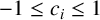 $-1\leq c_i \leq 1$
and
 $i=1,2,\ldots ,s$
. Here, we consider SDIMSIMs as a subclass of SGLMs which were introduced by Abdi et al. [Reference Abdi, Braś and Hojjati3]. These methods have the feature that
 $p=r=s$
and
 $q=p$
or
 $q=p-1$
with
 $U=I_s$
and V as a rank one matrix of the form
 $V=ev^T$
,
 $e=[1\hspace {2mm}1\hspace {2mm}\ldots \hspace {2mm}1]^T\in \mathbb {R}^s$
,
 $v=[v_1\hspace {2mm}v_2\hspace {2mm}\ldots \hspace {2mm}v_s]^T\in \mathbb {R}^s$
, with
 $v^Te=1$
.
3 Monotonicity theory for SGLMs based on Taylor series conditions
Reformulating the explicit SGLMs (2.2) as
 $$ \begin{align} \begin{array}{l} Y_i^{[n]} =\displaystyle \sum_{j=1}^{l}s_{ij}y_j^{[n-1]}+h \sum_{j=1}^{m}t_{ij} F (t_{n-1}+c_jh,Y_j^{[n]}) \\[3mm] \qquad \quad +\,h^2\displaystyle\sum_{j=1}^{m}\overline{t}_{ij}G (t_{n-1}+c_jh,Y_j^{[n]}),\quad i=1,2,\ldots,m, \\[3mm] y_i^{[n]} = Y_{m-l+i}^{[n]},\quad i=1,2,\ldots,l, \end{array} \end{align} $$
 $n=1,2,\ldots ,N$
,
 $1\leq l\leq m$
, sufficient conditions for SGLMs to preserve the strong stability properties of spatial discretizations are derived, provided that the forward Euler condition
 $$ \begin{align} \lVert Y^{[n]}+\Delta t F(Y^{[n]})\rVert\leq \lVert Y^{[n]}\rVert,\quad 0\leq\Delta t\leq\Delta t_{FE}, \end{align} $$
for any
 $\Delta t\leq \Delta t_{FE}$
, and the second derivative condition
 $$ \begin{align} \lVert Y^{[n]}+\Delta t^2G(Y^{[n]})\rVert\leq \lVert Y^{[n]}\rVert,\quad \Delta t\leq \widetilde{K}\Delta t_{FE}, \end{align} $$
to approximate the second derivative in time
 $u_{tt}$
, are satisfied. Here,
 $\widetilde {K}$
is a scaling factor comparing the stability condition of the second derivative term to that of the forward Euler term. The main drawback of using this pair of base conditions is that many common spatial discretization do not satisfy the condition (3.3), so that the schemes in [Reference Moradi, Abdi and Farzi34–Reference Moradi, Farzi and Abdi36], satisfying this pair of conditions, are not effective. Due to this reason, following the ideas of Ditkowski et al. [Reference Ditkowski, Gottlieb and Grant16] and Grant et al. [Reference Grant, Gottlieb and Seal22], we extend the alternative approach described in [Reference Grant, Gottlieb and Seal22] for SGLMs that allows the development of such methods which are SSP in the sense that they preserve the forward Euler condition (3.2) and Taylor series condition
 $$ \begin{align} \lVert Y^{[n]}+\Delta t F(Y^{[n]})+\tfrac{1}{2}\Delta t^2G(Y^{[n]})\rVert\leq \lVert Y^{[n]}\rVert,\quad \Delta t\leq K\Delta t_{FE}. \end{align} $$
Note that, as in [Reference Grant, Gottlieb and Seal22], any spatial discretization that satisfies the forward Euler and second derivative conditions (3.2) and (3.3) will also satisfy the Taylor series condition (3.4). Our goal in this paper is to develop explicit SGLMs of the form (3.1) that preserve the strong stability properties of forward Euler and Taylor series terms, perhaps under a different time-step condition
 $ \Delta t\leq \mathcal {C}_{TS}\Delta t_{FE}$
. To do this, we need different SSP conditions from those proposed by Moradi et al. [Reference Moradi, Farzi and Abdi36]. Such conditions for a given time-step are determined in the following theorem.
Theorem 1. Given spatial discretizations F and G that satisfy (3.2) and (3.4), an SGLM of the form (3.1) preserves the SSP property
 $\lVert Y^{[n+1]}\rVert \leq \lVert Y^{[n]}\rVert $
under the time-step condition
 $\Delta t\leq \gamma \Delta t_{FE}$
if the following conditions hold:
 $$ \begin{align} & \bigg(I+\gamma {T}+2\frac{\gamma ^2}{K^2}(1-K)\overline{T}\bigg)^{-1}{S} \geq 0, \!\qquad\qquad\quad \end{align} $$
 $$ \begin{align} & \gamma \bigg(I+\gamma {T}+2\frac{\gamma ^2}{K^2}(1-K)\overline{T}\bigg)^{-1}\bigg({T}-2\frac{\gamma}{K} \overline{T}\bigg) \geq 0, \end{align} $$
 $$ \begin{align} &2\frac{\gamma ^2}{K^2}\bigg(I+\gamma {T}+2\frac{\gamma ^2}{K^2}(1-K)\overline{{T}}\bigg)^{-1}\overline{T} \geq 0, \!\qquad\quad\end{align} $$
for some
 $\gamma>0$
. In the above conditions, the inequalities are understood component- wise.
Proof. Adding the term
 $(\gamma {T}+2\widehat {\gamma }(\,\widehat {\gamma }-\gamma )\overline {T})Y^{[n]}$
to both sides of method (3.1) leads to
 $$ \begin{align*} (I+\gamma {T}+2\widehat{\gamma }(\,\widehat{\gamma }-\gamma)\overline{T})Y^{[n]} &= {S}y^{[n-1]}+\gamma ({T}-2\widehat{\gamma}\,\overline{T})\bigg(Y^{[n]} + \frac{\Delta t}{\gamma }F\bigg) \\ &\quad+2\widehat{\gamma }^2\overline{T}\bigg(Y^{[n]}+\frac{\Delta t}{\widehat{\gamma}}F+\frac{\Delta t^2}{2\widehat{\gamma}^2}G\bigg). \end{align*} $$
Assuming that the matrix
 $(I+\gamma {T}+2\widehat {\gamma }(\,\widehat {\gamma }-\gamma )\overline {T})$
is invertible, we obtain
 $$ \begin{align} Y^{[n]} &= \mathbf{R}y^{[n-1]}+\mathbf{P}\bigg(Y^{[n]}+\frac{\Delta t}{\gamma }F\bigg)+\mathbf{Q}\bigg(Y^{[n]}+\frac{\Delta t}{\widehat{\gamma}}F+\frac{\Delta t^2}{2\widehat{\gamma }^2}G\bigg), \end{align} $$
with
 $$ \begin{align*} \begin{array}{l} \mathbf{R} = (I+\gamma {T}+2\widehat{\gamma }(\,\widehat{\gamma }-\gamma)\overline{T})^{-1}{S},\quad \mathbf{P} = \gamma (I+\gamma {T}+2\widehat{\gamma }(\,\widehat{\gamma }-\gamma)\overline{T})^{-1}({T}-2\widehat{\gamma}\,\overline{T}),\\ \\ \mathbf{Q} = \widehat{\gamma }(I+\gamma {T}+2\widehat{\gamma }(\,\widehat{\gamma }-\gamma)\overline{T})^{-1}\overline{T}. \end{array} \end{align*} $$
The relation (3.8) determines a convex combination of terms which are SSP, if
 $\mathbf {R}+\mathbf {P}+\mathbf {Q}=I$
and the elements of
 $\mathbf {R}$
,
 $\mathbf {P}$
and
 $\mathbf {Q}$
are all nonnegative. Therefore, the resulting value is SSP as well, that is,
 $$ \begin{align*} \lVert Y^{[n]}\rVert \leq \mathbf{R} \lVert y^{[n-1]}\rVert+\mathbf{P}\bigg\lVert Y^{[n]}+\frac{\Delta t}{\gamma }F\bigg\rVert + \mathbf{Q}\bigg\lVert Y^{[n]}+\frac{\Delta t}{\widehat{\gamma}}F+\frac{\Delta t^2}{2\widehat{\gamma }}G\bigg\rVert, \end{align*} $$
under the time-step restrictions
 $\Delta t\leq \gamma \Delta t_{FE}$
and
 $\Delta t\leq K\,\widehat {\gamma }\Delta t_{FE}$
. To obtain the optimal time-step, these two time-step restrictions must be set equal, and so we require
 $\gamma =K\,\widehat {\gamma }$
. Therefore, for
 $\widehat {\gamma }=\gamma /K$
, conditions (3.5)–(3.7) ensure that
 $\mathbf {R}\geq 0$
,
 $\mathbf {P}\geq 0$
and
 $\mathbf {Q}\geq 0$
component-wise, and the method (3.1) preserves the strong stability condition
 $\lVert Y^{[n+1]}\rVert \leq \lVert Y^{[n]}\rVert $
under the time-step restriction
 $\Delta t\leq \gamma \Delta t_{FE}$
. This completes the proof of the theorem.
This theorem allows us to formulate the search for optimal SSP SGLMs as an optimization problem which maximize the value of the SSP coefficient
 $\mathcal {C}_{TS}$
subject to the SSP conditions (3.5)–(3.7).
In a similar way to [Reference Moradi, Farzi and Abdi36], the SSP conditions (3.5)–(3.7) can be reformulated in terms of the coefficient matrices A,
 $\overline {A}$
, U, B,
 $\overline {B}$
and V of SGLMs (2.2). Using the same process discussed in [Reference Moradi, Farzi and Abdi36], these conditions are equivalent to
 $$ \begin{align} \left\{\begin{aligned} & \bigg(I+\gamma A+2\frac{\gamma^2}{K^2}(1-K)\overline{A}\bigg)^{-1}U\geq0, \\[1mm] & \gamma\bigg(I+\gamma A+2\frac{\gamma^2}{K^2}(1-K)\overline{A}\bigg)^{-1}\bigg(A-2\frac{\gamma}{K}\overline{A}\bigg)\geq0, \\[1mm] & V-\bigg(\gamma B+2\frac{\gamma^2}{K^2}(1-K)\overline{B}\bigg)\bigg(I+\gamma A+2\frac{\gamma^2}{K^2}(1-K)\overline{A}\bigg)^{-1}U\geq0, \\[1mm] & \gamma \bigg(B-2\frac{\gamma}{K}\overline{B}\bigg)-\gamma\bigg(\gamma B+2\frac{\gamma^2}{K^2}(1-K)\overline{B}\bigg)\bigg(I+\gamma A+2\frac{\gamma^2}{K^2}(1-K)\overline{A}\bigg)^{-1}\bigg(A-2\frac{\gamma}{K}\overline{A}\bigg)\geq0, \\[1mm] & 2\frac{\gamma^2}{{K}^2}\bigg(I+\gamma A+2\frac{\gamma^2}{K^2}(1-K)\overline{A}\bigg)^{-1}\overline{A}\geq0, \\[1mm] & 2\frac{\gamma^2}{{K}^2}\overline{B}-2\frac{\gamma^2}{K^2}\bigg(\gamma B+2\frac{\gamma^2}{K^2}(1-K)\overline{B}\bigg)\bigg(I+\gamma A+2\frac{\gamma^2}{K^2}(1-K)\overline{A}\bigg)^{-1}\overline{A}\geq0, \end{aligned} \right. \end{align} $$
where K can be any positive constant, and the SSP coefficient
 $\mathcal {C}_{TS}$
for SGLMs (2.2) can be obtained by
 $$ \begin{align*} \mathcal{C}_{TS}=\mathcal{C}_{TS}(c,A,\overline{A},U,B,\overline{B},V)=\sup\, \{\gamma \in\mathbb{R}\mid \gamma \text{ satisfies}\ (3.9)\}. \end{align*} $$
The results obtained in the following section indicate that considering these new SSP conditions leads to the methods that not only increase our flexibility in the choice of spatial discretizations but also have larger SSP coefficients than those of the methods studied in [Reference Ditkowski, Gottlieb and Grant16, Reference Grant, Gottlieb and Seal22, Reference Moradi, Abdi and Farzi34–Reference Moradi, Farzi and Abdi36]. In this paper, we refer to SSP-TS SGLMs as the SGLMs preserving strong stability properties of (3.2) and (3.4), and to SSP-SD SGLMs as the SGLMs preserving strong stability properties of (3.2) and (3.3).
4 Derivation of SSP SDIMSIMs based on Taylor series conditions
In this section, we search for SSP SDIMSIMs that preserve the SSP properties (3.9). The SSP coefficient of the obtained methods of order
 $p=r=s$
and stage order
 $q=p$
and
 $q=p-1$
up to order eight are presented. The structure of order conditions for such methods were discussed by Abdi et al. [Reference Abdi and Behzad2, Reference Abdi, Braś and Hojjati3]. Define
 $Z=[1\ z\ \cdots\ z^p]^T\in \mathbb {C}^{p+1}$
and the matrix
 $$ \begin{align*}W=[\alpha_0\ \alpha_1\ \cdots\ \alpha_p]\end{align*} $$
with the vectors
 $\alpha _k$
,
 $k=0,1,\ldots ,p$
, defined by
 $\alpha _k=[\alpha _{1k}\ \alpha _{2k}\ \cdots \ \alpha _{rk}]^T$
.
In the case of methods with
 $p=q$
, Abdi et al. [Reference Abdi, Braś and Hojjati3] determined that the stage order and order conditions are given by
 $$ \begin{align} \quad\, e^{cz}&=zAe^{cz}+z^2\overline{A}e^{cz}+UWZ+O(z^{p+1}), \end{align} $$
 $$ \begin{align} e^zWZ &=zBe^{cz}+z^2\overline{B}e^{cz}+VWZ+O(z^{p+1}). \end{align} $$
Moreover, an SGLM has order p and stage order
 $q=p-1$
if and only if [Reference Abdi and Behzad2]
 $$ \begin{align} e^{cz}&=zAe^{cz}+z^2\overline{A}e^{cz}+UWZ \nonumber\\ &\quad+\bigg(\frac{c^p}{p!}-A\frac{c^{p-1}}{(\kern1.1pt p-1)!}-\overline{A}\frac{c^{p-2}}{(\kern1.1pt p-2)!}-U\alpha_p\bigg)z^p+O(z^{p+1}), \end{align} $$
 $$ \begin{align} e^zWZ&=zBe^{cz}+z^2\overline{B}e^{cz}+VWZ+O(z^{p+1}). \!\!\!\qquad\quad\qquad\qquad\qquad \end{align} $$
Here, the exponential function is applied componentwise to a vector. If we choose
 $U=I_s$
, the stage order conditions (4.1) and (4.3) are given by
 $$ \begin{align} W=C-ACK-\overline{A}CK^2,\quad \widehat{W}=\widehat{C}-AC\widehat{K}-\overline{A}CK\widehat{K}, \end{align} $$
respectively, where
 $C=(C_{ij})\in \mathbb {R}^{s\times (\kern1.1pt p+1)}$
is the Vandermonde matrix [Reference Horn and Johnson25] with elements
 $$ \begin{align*}C_{ij}=\frac{c_i^{\,j-1}}{(\,j-1)!},\quad 1\leq i\leq s,\quad 1\leq j\leq p+1,\end{align*} $$
 $K\in \mathbb {R}^{(\kern1.1pt p+1)\times (\kern1.1pt p+1)}$
is the shifting matrix defined by
 $K=[0\ \, e_1\ \, \cdots \ \, e_p]$
with
 $e_j$
as the jth unit vector in
 $\mathbb {R}^{p+1}$
and the matrix
 $\widehat {X}$
refers to the matrix obtained by the p first columns of a given matrix X.
For such methods, the order conditions lead to a formula for the coefficient matrix B in terms of c, A,
 $\overline {A}$
,
 $\overline {B}$
and V as
 $$ \begin{align*} B=B_0-AB_1-\overline{A}B_2-VB_3-(\overline{B}-V\overline{A})B_4+VA, \end{align*} $$
for the case with
 $p=q=r=s$
[Reference Abdi, Braś and Hojjati3], and
 $$ \begin{align} B &= B_0-AB_1-\overline{A}B_2-VB_3-(\overline{B}-V\overline{A})B_4+VA \nonumber\\ &\quad -\bigg(\frac{c^p}{p!}-A\frac{c^{p-1}}{(\kern1.1pt p-1)!}-\overline{A}\frac{c^{p-2}}{(\kern1.1pt p-2)!}-\alpha_p\bigg)e^TB_5 \nonumber \\ &\quad +V\bigg(\frac{c^p}{p!}-A\frac{c^{p-1}}{(\kern1.1pt p-1)!}-\overline{A}\frac{c^{p-2}}{(\kern1.1pt p-2)!}-\alpha_p\bigg)e^TB_6, \end{align} $$
for methods with
 $p=q+1=r=s$
[Reference Moradi, Sharifi and Abdi38], where the
 $(i,j)$
elements of
 $B_0$
,
 $B_1$
,
 $B_2$
,
 $B_3$
,
 $B_4$
,
 $B_5$
and
 $B_6$
are respectively given by
 $$ \begin{align*} \begin{aligned} & \frac{\int_{0}^{1+c_i}\phi_j(x)dx}{\phi_j(c_j)},\quad \frac{\phi_j(1+c_i)}{\phi_j(c_j)},\quad \frac{\phi_j'(1+c_i)}{\phi_j(c_j)},\quad \frac{\int_{0}^{c_i}\phi_j(x)dx}{\phi_j(c_j)},\\ \nonumber &\frac{\phi_j'(c_i)}{\phi_j(c_j)},\quad \frac{(\kern1.1pt p-1)!}{\phi_j(c_j)},\quad \frac{(\kern1.1pt p-1)!}{\phi_j(c_j)}, \end{aligned} \end{align*} $$
and
 $\phi _i(x)$
is defined by
 $$ \begin{align*}\phi_i(x)=\prod_{j=1,j\neq i}^{s}(x-c_j),\quad i=1,2,\ldots,s.\end{align*} $$
After an extensive search to obtain SSP SDIMSIMs, we observed that for such methods, the matrices A and
 $\overline {A}$
are identically equal to the zero matrix. Although these methods have SSP properties, their SSP coefficients are too small and are not optimal. So, as in [Reference Moradi, Abdi and Farzi34], to obtain methods with large SSP coefficients
 $\mathcal {C}_{TS}$
, we will consider a more general class of transformed SDIMSIMs. Introducing T as a nonsingular transformed matrix and multiplying the relation for
 $y^{[n]}$
by
 $T\otimes I_m$
, where
 $\otimes $
is the Kronecker product of two matrices, lead to the class of transformed methods defined by
 $$ \begin{align} \begin{aligned} & Y^{[n]}= h(A\otimes I_m)f(Y^{[n]})+h^2(\overline{A}\otimes I_m)g(Y^{[n]})+(UT^{-1}\otimes I_m)(T\otimes I_m)y^{[n-1]},\\[6pt] & (T\otimes I_m)y^{[n]}=h(TB\otimes I_m)f(Y^{[n]})+h^2(T\overline{B}\otimes I_m)g(Y^{[n]})\\[6pt] &\qquad \qquad \qquad +(TVT^{-1}\otimes I_m)(T\otimes I_m)y^{[n-1]}. \end{aligned} \end{align} $$
Now, introducing
 $$ \begin{align*}\widetilde{y}^{\,[n]}=(T\otimes I_m)y^{[n]},\quad \widetilde{y}^{\,[n-1]}=(T\otimes I_m)y^{[n-1]},\end{align*} $$
results in the following form of (4.7):
 $$ \begin{align} \begin{array}{c} Y^{[n]}=h(A\otimes I_m)f(Y^{[n]})+h^2(\overline{A}\otimes I_m)g(Y^{[n]})+(\widetilde{U}\otimes I_m)\widetilde{y}^{\,[n-1]}, \\[6pt] \widetilde{y}^{\,[n]}=h(\widetilde{B}\otimes I_m)f(Y^{[n]})+h^2(\widetilde{\overline{B}}\otimes I_m)g(Y^{[n]})+(\widetilde{V}\otimes I_m)\widetilde{y}^{\,[n-1]}, \end{array} \end{align} $$
where the transformed coefficient matrices
 $\widetilde {U}$
,
 $\widetilde {B}$
,
 $\widetilde {\overline {B}}$
and
 $\widetilde {V}$
are given by
 $$ \begin{align*}\widetilde{U}=UT^{-1},\quad \widetilde{B}=TB,\quad \widetilde{\overline{B}}=T\overline{B},\quad \widetilde{V}=TVT^{-1}.\end{align*} $$
With respect to the transformed starting procedure
 $$ \begin{align*} \widetilde{y}^{[0]}=\sum_{k=0}^{p}(\widetilde{\alpha}_k\otimes I)h^ky^{(k)}(t_0)+O(h^{p+1}), \end{align*} $$
where
 $\widetilde {\alpha }_k =T\alpha _k, k=0,1,\ldots ,p$
, the transformed SDIMSIMs (4.8) preserves the order p, the stage order
 $q=p$
and
 $q=p-1$
of the original methods (2.2). Now to obtain SSP SDIMSIMs based on Taylor series conditions, we search for such methods by solving the minimization problem (2.3) subject to the nonlinear components inequality
 $$ \begin{align} \left\{\begin{aligned} & \bigg(I+\gamma A+2\frac{\gamma^2}{K^2}(1-K)\overline{A}\bigg)^{-1}\widetilde{U}\geq0, \\[1mm] & \gamma\bigg(I+\gamma A+2\frac{\gamma^2}{K^2}(1-K)\overline{A}\bigg)^{-1}\bigg(A-2\frac{\gamma}{K}\overline{A}\bigg)\geq0, \\[1mm] & \widetilde{V}-\bigg(\gamma \widetilde{B}+2\frac{\gamma^2}{K^2}(1-K)\widetilde{\overline{B}}\bigg)\bigg(I+\gamma A+2\frac{\gamma^2}{K^2}(1-K)\overline{A}\bigg)^{-1}\widetilde{U}\geq0 , \\[1mm] & \gamma \bigg(\widetilde{B}-2\frac{\gamma}{K}\widetilde{\overline{B}}\bigg)-\gamma\bigg(\gamma \widetilde{B}+2\frac{\gamma^2}{K^2}(1-K)\widetilde{\overline{B}}\bigg)\bigg(I+\gamma A+2\frac{\gamma^2}{K^2}(1-K)\overline{A}\bigg)^{-1}\bigg(A-2\frac{\gamma}{K}\overline{A}\bigg)\geq0, \\[1mm] & 2\frac{\gamma^2}{{K}^2}\bigg(I+\gamma A+2\frac{\gamma^2}{K^2}(1-K)\overline{A}\bigg)^{-1}\overline{A}\geq0, \\[1mm] & 2\frac{\gamma^2}{{K}^2}\widetilde{\overline{B}}-2\frac{\gamma^2}{K^2}\bigg(\gamma \widetilde{B}+2\frac{\gamma^2}{K^2}(1-K)\widetilde{\overline{B}}\bigg)\bigg(I+\gamma A+2\frac{\gamma^2}{K^2}(1-K)\overline{A}\bigg)^{-1}\overline{A}\geq0, \end{aligned} \right. \end{align} $$
where
 $\gamma $
is some constant and K can take any positive value. For these methods, the SSP coefficient
 $\mathcal {C}_{TS}$
is given by
 $$ \begin{align} \mathcal{C}_{TS}=\mathcal{C}_{TS}(c,A,\overline{A},\widetilde{U},\widetilde{B},\widetilde{\overline{B}}, \widetilde{V})= \sup\,\{\gamma\in\mathbb{R} \mid \gamma \text{ satisfies}\ (4.9)\}. \end{align} $$
In the rest of this section, we will consider the base conditions (3.2) and (3.4), and use the characterization (4.10) of the SSP coefficient
 $\mathcal {C}_{TS}$
to search for new SSP schemes with larger SSP coefficient than those for other existing SSP methods. Furthermore, to compare the overall efficiency of methods for a given order and different number of stages s, we also report the effective SSP coefficient defined by
 $\mathcal {C}_{ff}=C/s$
. In what follows, we refer to SSP-TS SDIMSIMs
 $_{pq}$
as the SSP SDIMSIMs based on Taylor series conditions and to SSP-SD SDIMSIMs
 $_{pq}$
as the SSP SDIMSIMs based on second derivative conditions, where p is the order of the method and q is the stage order. The aim of this paper is to obtain high order SSP schemes based on Taylor series conditions up to order eight. Solving the stage order and order conditions (4.5)–(4.6) leads to the SDIMSIMs of order p and stage order
 $q=p$
or
 $q=p-1$
with entries of A,
 $\overline {A}$
,
 $\overline {B}$
and V, together with
 $c_i$
,
 $i=1,2,\ldots ,s$
, as free parameters. Now, to obtain SSP-TS SDIMSIMs, we consider all of these free parameters, in addition to the unknown parameters of nonsingular transformation matrix T, to the minimization problem (2.3) subject to the nonlinear inequality constraints (4.9), and solve this optimization problem using the fmincon command with the sequential quadratic programming (SQP) algorithm from MATLAB and with many random starting points.
As a simple example that provides optimal formulations with simple formulae, we consider the strong stability properties of second order methods with
 $p=q=r=s$
and abscissa vector
 $c=[1/2 \hspace {2mm}1]^T$
. The coefficient matrices of the original SDIMSIMs are in the form
 $$ \begin{align*}\left[\begin{array}{c|c|c} A & \overline{A} & U \\ \hline B & \overline{B} & V \end{array}\right]=\left[\begin{array}{cc|cc|cc} 0 & 0 & 0 & 0 & 1 & 0 \\ a_{21} & 0 & \overline{a}_{21} & 0 & 0 & 1 \\ \hline b_{11} & b_{12} & \overline{b}_{11} & \overline{b}_{12} & 1-v & v \\ b_{21} & b_{22} & \overline{b}_{21} & \overline{b}_{22} & 1-v & v \end{array}\right]. \end{align*} $$
Solving the order and stage order conditions and a straightforward SSP analysis with the nonzero entries of A,
 $\overline {A}$
, the entries of
 $\overline {B}$
and v, together with four unknown parameters of nonsingular transformation matrix T,
 $[t_{ij}]_{i,j=1}^r$
, as free parameters enable us to formulate the optimal methods without the use of optimization code. The coefficients of the method are given by
 $$ \begin{align*}\begin{array}{l} a_{21} = \dfrac{(K-1)t_{22}-t_{21}}{\gamma t_{22}},\quad\overline{a}_{21}=\dfrac{K^2}{2\gamma^2},\quad \overline{b}_{11}=\overline{b}_{12}=\overline{b}_{21}=\overline{b}_{22}=\dfrac{1}{8},\\[3mm] v=\dfrac{2K(\gamma+1)+3\gamma^2+\gamma}{K(\gamma+2)+\gamma(2\gamma+3)},\quad t_{11}=\dfrac{8}{3\gamma},\quad t_{12}=0,\\[5mm] t_{21}=\dfrac{t_{22} (-3\gamma^3+(3K-6) \gamma^2+2\gamma(K^2+2K-2))}{\gamma(\gamma^2+3\gamma+4)},\quad t_{22}=\dfrac{t_{11}(3K-2)}{(5K+4)}, \end{array}\end{align*} $$
with
 $\gamma = 2K$
.
The SSP coefficients of the proposed methods depending on the value of K are listed in Tables 1–5, using the notation TS-SDIMSIM
 $_{pq}$
. In these tables, to compare our methods with the SSP two-derivative RK (TDRK) methods studied in [Reference Grant, Gottlieb and Seal22], the SSP coefficients of these methods, using the notation TS-TDRK
 $_{pq}$
, are also listed with the same number of internal stages s. It is obvious that the SSP coefficient of SSP SGLMs is dependent on the value of K which comes from the SSP conditions. Indeed, increasing the value of K results in the increase of the SSP coefficients. However, there is a trade-off between the SSP coefficient and stage order of the methods. In other words, for a given order p, the SSP coefficient of the method decreases as the stage order increases. In the case of order four, from Table 2, one can see that for
 $K<1$
, the SSP coefficients are greater than those of the SSP-TS TDRK methods with stage order
 $q=2$
, for
 $K=1$
, the SSP coefficient of SSP-TS SDIMSIMs with
 $q=p$
is close to that of the SSP-TS TDRK method but those for SSP-TS SDIMSIMs with
 $q=p-1$
are greater; but for
 $K>1$
, SSP-TS SDIMSIMs have smaller SSP coefficients than those for the SSP-TS TDRK method. In the case of order five, the SSP coefficients of the optimal SSP-TS SDIMSIMs for
 $K\geq 1$
are smaller than those of the SSP-TS TDRK with the same order and stage order
 $q=2$
. For
 $p=6$
, the optimal SSP-TS SDIMSIMs for
 $q=p$
and
 $q=p-1$
, we found that the all SSP-TS SDIMSIMs have larger SSP coefficients than those of the corresponding SSP-TS TDRK methods for each K. As a matter of fact, for a given order p, SSP coefficients for low stage order methods have larger SSP coefficients than those of the corresponding high stage order methods. Along with this fact, we expect that SSP-TS SDIMSIMs with low stage order,
 $q\leq p-2$
, provide even larger SSP coefficients than those reported here. Although it is possible to find such methods, these require different order and stage order conditions stated in this paper, and so we only focus on constructing SSP-TS SDIMSIMs with stage order
 $q=p$
and
 $q=p-1$
. In the case of the methods with
 $p=q=r=s$
, after an extensive search, we were not able to find SSP-TS SDIMSIMs with
 $p=8$
. For a single value of K, chosen by
 $K=1$
, the effective SSP coefficient
 $\mathcal {C}_{\text {eff}}$
for the proposed methods are listed in Table 6, using the notation TS-SDIMSIM
 $_{pq}$
. For the sake of comparison, we have also listed the effective SSP coefficient
 $\mathcal {C}_{\text {eff}}$
for SSP methods investigated in [Reference Moradi, Abdi and Farzi34], and [Reference Ditkowski, Gottlieb and Grant16] using the notation SD-SDIMSIM
 $_{pq}$
(SSP SDIMSIM based on second derivative conditions) and TS-SGLM
 $_{pq}$
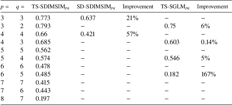
, respectively. By Table 6, we see that the improvement in the SSP-TS SDIMSIMs compared with the SSP-SD SDIMSIMs studied in [Reference Moradi, Abdi and Farzi34] ranges from 21% to 57%. Moreover, this table shows improvement in the range of 5% to 167% compared with the SSP-TS SGLMs investigated in [Reference Ditkowski, Gottlieb and Grant16]. Note that in this table, dashes indicate that such methods are not provided in [Reference Ditkowski, Gottlieb and Grant16, Reference Moradi, Abdi and Farzi34], so that there is no percentage improvement available in the SSP coefficients.
SSP-TS coefficients of SDIMSIMs with
 $p=r=s=3$
and
 $q=3,2$
.

SSP-TS coefficients of SDIMSIMs with
 $p=r=s=4$
and
 $q=4,3$
together with those for SSP-TS TDRK methods with
 $p=s=4$
and
 $q=2$
.

SSP-TS coefficients of SDIMSIMs with
 $p=r=s=5$
and
 $q=5,4$
together with those for SSP-TS TDRK methods with
 $p=s=5$
and
 $q=2$
.

SSP-TS coefficients of SDIMSIMs with
 $p=r=s=6$
and
 $q=6,5$
together with those for SSP-TS TDRK methods with
 $p=s=6$
and
 $q=2$
.

SSP-TS coefficients of SDIMSIMs with
 $p=r=s=7,8$
and
 $q=7,6$
.

Effective SSP coefficients of the SSP-TS SDIMSIMs up to
 $p=8$
and
 $q=p$
and
 $q=p-1$
, compared with the SD-SDIMSIMs in [Reference Moradi, Abdi and Farzi34] and TS-SGLMs in [Reference Ditkowski, Gottlieb and Grant16]. The used value for K is
 $\sqrt {2}/2$
for the methods from [Reference Moradi, Abdi and Farzi34] and
 $K=1$
for the proposed methods in this work and the methods from [Reference Ditkowski, Gottlieb and Grant16].

The coefficient matrices of the constructed SSP-TS SDIMSIMs with
 ${p=q=r=s\leq 7}$
and
 $p=q+1=r=s=8$
for
 $K=1$
, used in our numerical experiments in Section 5, have been reported in the Appendix.
5 Numerical experiments
To illustrate the verification of the convergence order and the stability properties of the proposed methods in this work, we test our methods on several one-dimensional numerical experiments. In what follows, we first preview our results and then present them in more detail throughout the following subsections.
First, in Section 5.1, we are going to test our methods to verify the order of convergence. To accomplish this study, usually an appropriate starting procedure is required to obtain the expected order of convergence. In this paper, similar to the work in [Reference Moradi, Abdi and Farzi34–Reference Moradi, Farzi and Abdi36], to approximate the temporal derivatives, we adopt a Lax–Wendroff type approach which uses the PDEs (1.1) to replace the temporal derivatives by the spatial derivatives, and discretize them in space. The purpose of the tests in Section 5.2 is to focus on the verification of the SSP properties of the proposed methods in the presence of the shock. We consider two nonlinear scaler PDEs, inviscid Burgers equation [Reference Laney32] and the Buckley–Leverett equation [Reference LeVeque33], using fifth-order finite difference WENO method (WENO5) [Reference Jiang and Shu30], which is not provably total variation diminishing (TVD), for the spatial discretization. Our tests indicate that the proposed methods in this work perform significantly better than other existing methods in the presence of the shock, and preserve the SSP property with larger allowable time-step. In the rest of this subsection, we turn our attention to how the SSP properties of these methods are practically preserved, by considering the total variation of the numerical solutions. To accomplish this, we consider two scaler PDEs: the linear advection equation and Burger’s equation, using simple first-order spatial discretizations, which are provably TVD over time for the first derivative. Numerical results indicate that our methods preserve these properties as expected by the theory.
5.1 Convergence studies
To show the verification of the order of convergence, we consider a linear advection problem
 $u_t+u_x=0$
with periodic boundary conditions and initial condition
 $u_0(x)=0.5+0.5\sin (x)$
on the spatial domain
 $x\in [0,2\pi ]$
. Using the Fourier pseudospectral differential matrix D [Reference Hesthaven, Gottlieb and Gottlieb23] to discretize the spatial grids, we can approximate the first derivative
 $F\approx -u_x\approx -Du$
and the second derivative
 $F_t=u_{tt}=-DF=-D^2u=G$
without raising discretization errors. For one single value of
 $K=1$
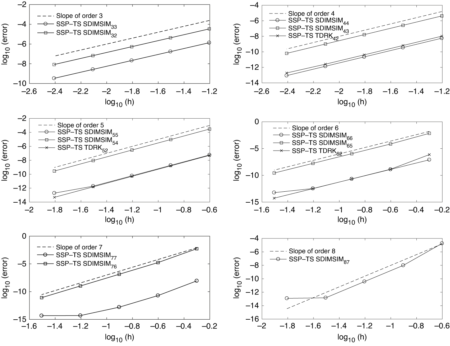
, in Figure 1, we have plotted the norm of global error at the final time
 $T_f=2.0$
in double logarithmic scale. These numerical results verify that the errors decrease with the expected theoretical orders. This illustrates that using the Lax–Wendroff type approach to approximate the temporal derivative does not influence the accuracy of the methods.
Order verification for SSP-TS SDIMSIM
 $_{pq}$
of order
 $p=r=s$
and stage order
 $q=p$
and
 ${q\,{=}\,p-1}$
with
 $K=1$
and grid refinement in time.

5.2 Monotonicity studies
In this subsection, we are going to verify the SSP properties of the constructed methods in the presence of the shock. To do this, we present some numerical experiments in conjunction with the WENO5 to discretize the spatial grids, along with the results obtained using the fourth-order SSP-SD SDIMSIM investigated by Moradi et al. [Reference Moradi, Abdi and Farzi34] and the SSP-TS TDRK method of order
 $p=s=4$
and stage order
 $q=2$
studied by Grant et al. [Reference Grant, Gottlieb and Seal22]. Here, after computing the approximation of
 $u_t^n$
, that is,
 $u_t^n=-f(u^n)_x$
by a WENO5 finite difference, to approximate
 $u_{tt}$
at the point
 $(x_j,t_n)$
, we use the following fourth-order central difference formula
 $$ \begin{align*} u_{j,tt}\approx -\frac{1}{12\Delta x} (g_{j-2}^n-8g_{j-1}^n+8g_{j+1}^n-g_{j+2}^n), \end{align*} $$
so that the calculation of second derivative functions does not lead to additional cost. Here
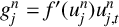 $g_j^n=f'(u_j^n)u_{j,t}^n$
, and
 $u_j^n$
and
 $u_{j,t}^n$
are the approximation of u at the points
 $(x_j,t_n)$
.
We consider the following problems.
Problem 1 (One-dimensional inviscid Burgers equation [Reference Laney32]).
We consider the following one-dimensional inviscid Burgers equation
 $$ \begin{align*} \frac{\partial u(x,t)}{\partial t}+\frac{\partial}{\partial x}\bigg(\frac{1}{2}u^2(x,t)\bigg)=0,\quad 0\leq x\leq X,\quad0\leq t\leq T_f. \end{align*} $$
-
(1) Smooth initial data.
We consider the initial condition
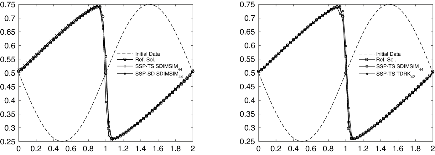
 $u(x,0)=1/2-(1/4)\sin (\pi x)$
, and periodic boundary conditions
$u(0,t)=u(X,t)$
with
$X=2.0$
and
$0\leq t \leq T_f$
. Taking a variable time-step
$\Delta t=\mathrm {CFL}(\Delta x/\max _i\lvert u(x_i)\rvert )$
with CFL=1.75 (
$N_t=26$
), we run the simulation up to
$T_f=2.0$
.
-
(2) Discontinuous initial data.
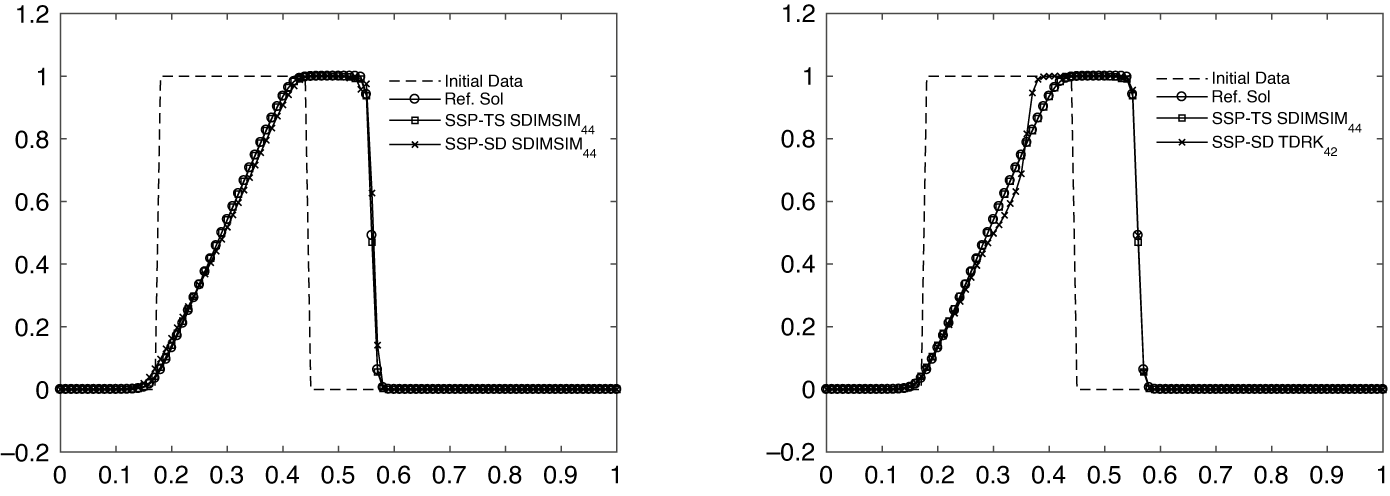
In this problem, we set the initial condition as
and periodic boundary conditions
$$ \begin{align*}u(x,0)=\left\{\begin{array}{@{}l} 1\quad \text{if } 0.18\leq x\leq 0.44 \\ 0\quad \text{otherwise}, \end{array} \right. \end{align*} $$
$u(0,t)=u(X,t)$
, with
$X=1.0$
and
$0\leq t\leq T_f$
. Using a variable time-step
$\Delta t=\mathrm {CFL}(\Delta x/\max _i\lvert u(x_i)\rvert )$
with CFL=2.2 (
$N_t=10$
), and a resolution of
$N=100$
points, we run the simulation up to
$T_f=0.23$
.













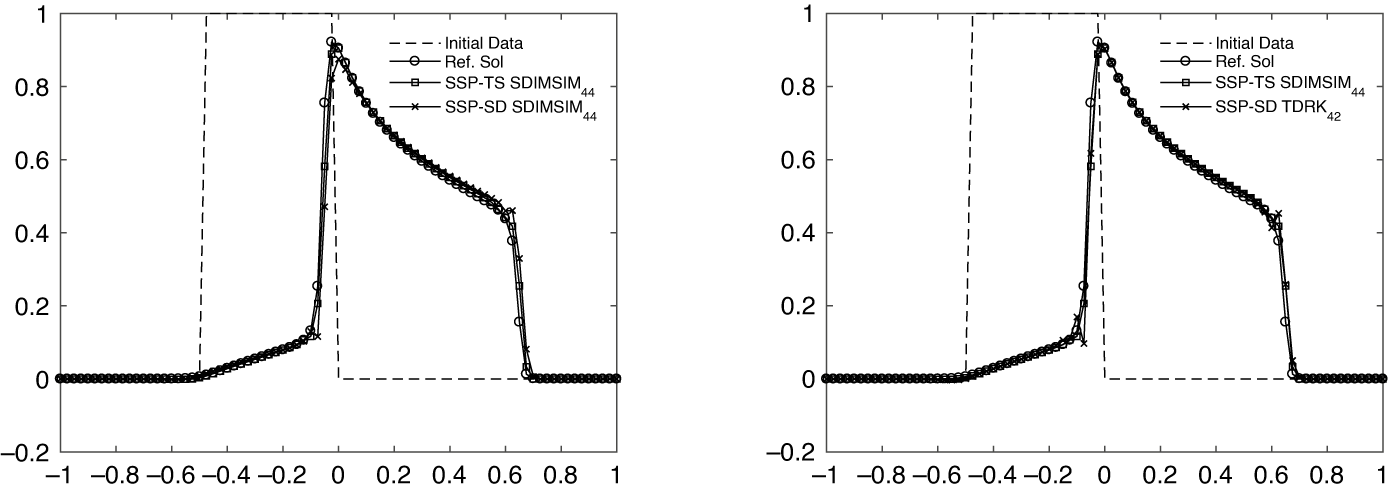
Problem 2 (Buckley–Leverett equation [Reference LeVeque33]).
The flux for the Buckley–Leverett equation
 $$ \begin{align*} \frac{\partial u(x,t)}{\partial t}+\frac{\partial}{\partial x} (\Phi(u(x,t)))=0,\quad -1\leq x\leq 1,\quad0\leq t\leq T_f, \end{align*} $$
is given by
 $$ \begin{align*} \Phi(u)=\frac{4u^2}{4u^2+(1-u)^2}, \end{align*} $$
with discontinuous initial condition
 $u(x,0)=1$
in
 $[-0.5,0]$
and
 $u(x,0)=0$
elsewhere, and periodic boundary conditions
 $u(-1,t)=u(1,t)$
,
 $0\leq t\leq T_f$
. We run this simulation using a constant time-step
 $\Delta t=\mathrm {CFL}(\Delta x/\max _i \lvert u(x_i)\rvert )$
with CFL=0.9 (
 $N_t=18$
) and a resolution of
 $N=80$
points.
In Figures 2, 3 and 4, we have plotted the obtained results by the SSP-TS SDIMSIM of order
 $p=4$
. Moreover, to show the efficiency of the proposed methods, we have also plotted the numerical results of the SSP-TS SDIMSIM
 $_{pq}$
with
 $p=q=4$
, and the SSP-TS TDRK
 $_{pq}$
method with order
 $p=4$
and stage order
 $q=2$
, using the same temporal stepsize
 $\Delta t$
for all the methods. From the numerical results presented in Figures 2, 3 and 4, we observe that the SSP-TS SDIMSIM
 $_{44}$
in the presence of shock, performs better and does not generate the spurious oscillations.
Numerical results of different SSP methods for Problem 1 with smooth solution at
 $T_f=2.0$
and
 $N=80$
.

Numerical results of different SSP methods for Problem 1 with discontinuous solution at
 $T_f=0.23$
.

Numerical results of different SSP methods for Problem 2 with discontinuous solution at
 $T_f=0.4$
.

Problem 3 (Euler systems).
In this test, we assess the performance of SSP-TS SDIMSIM
 $_{44}$
used in conjunction with the approximate Riemann problem. We consider four Riemann initial conditions for the one-dimensional Euler equations for ideal gases with
 $\gamma =1.4$
. These cases are considered to show some typical wave behaviours from the solution of the Riemann problem [Reference Toro43]. The one-dimensional Euler equations [Reference Qiu and Shu39] are a nonlinear system of hyperbolic conservation laws defined by
 $$ \begin{align*} U_t+F(U)_x=0, \end{align*} $$
with
 $$ \begin{align*} U^T&= (\,\rho,\rho v,E)^T, \\ F(U)&= (\,\rho v,\rho v^2+\mathbf{p},v(E+\mathbf{p}))^T. \end{align*} $$
Here
 $\rho $
, E, v and
 $\mathbf {p}$
stand for the density, the total energy, the velocity and the pressure, respectively, related to the total energy
 $$ \begin{align*} E=\frac{\mathbf{p}}{\gamma-1}+\frac{1}{2}\rho(v^2). \end{align*} $$
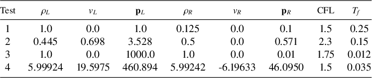
Table 7 gives the data for all four tests. In all cases, data consist of two constant states
 $U_L=[\,\rho _L,v_L,\mathbf {p}_L]^T$
and
 $U_R=[\,\rho _R,v_R,\mathbf {p}_R]^T$
, separated by a discontinuity. We run this simulation using a variable time-step
 $\Delta t=\mathrm {CFL}(\Delta x/\max _i\lvert u(x_i)\rvert )$
and a resolution of
 $N=100$
points.
Data for four Riemann problem tests.

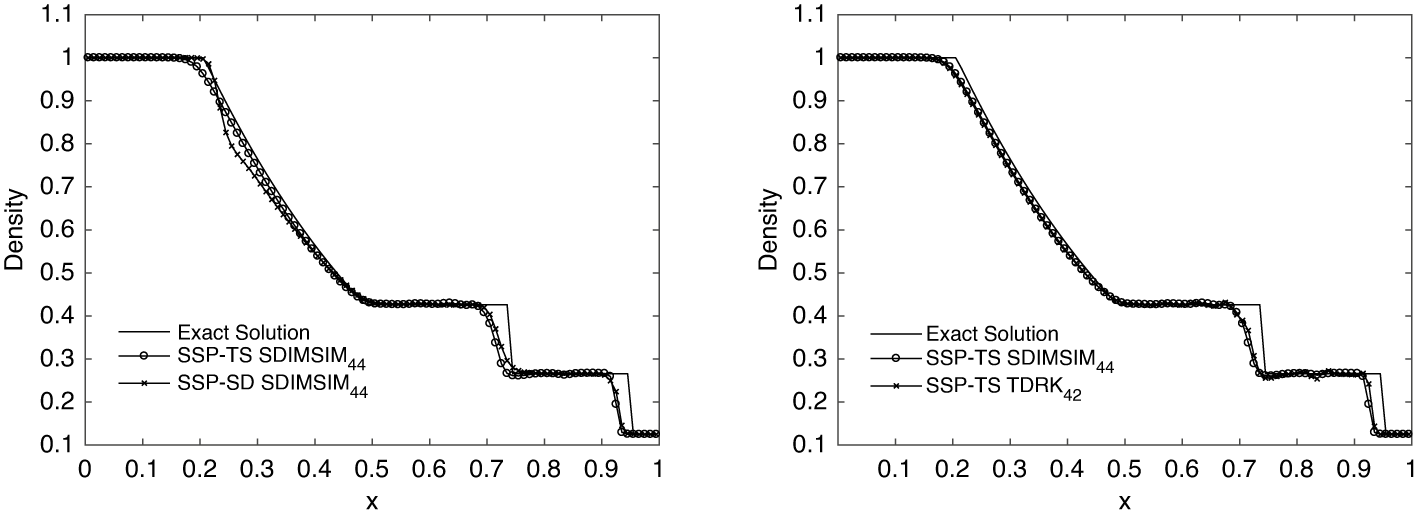
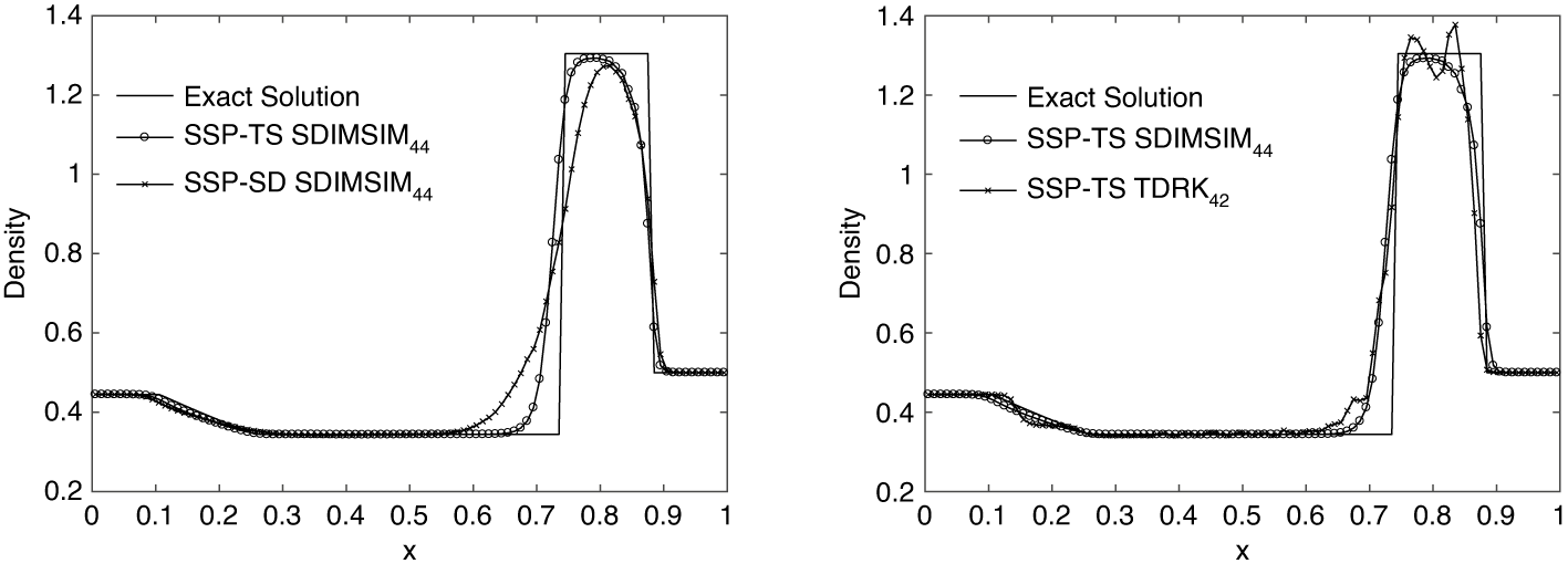
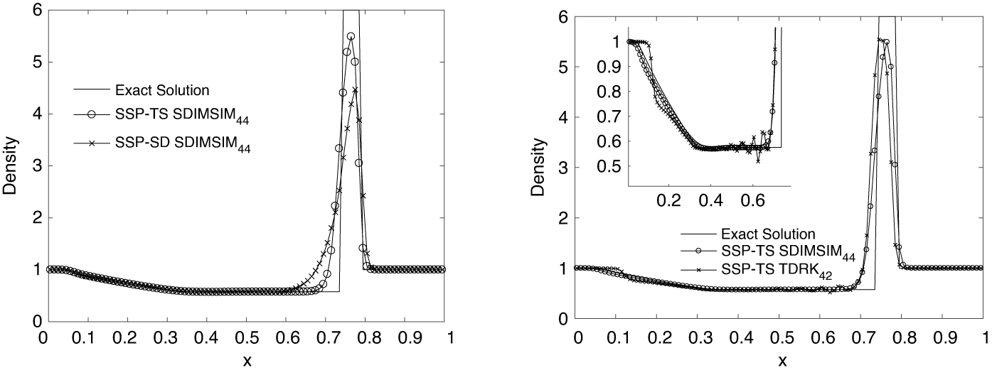
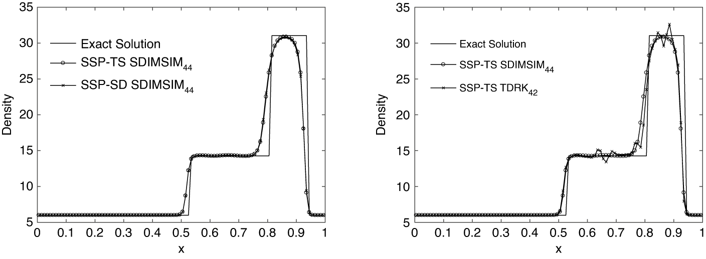
In Figures 5, 6, 7 and 8, we have plotted the numerical results for the density obtained by the SSP-TS SDIMSIM of order
 $p=4$
, together with that for SSP-SD SDIMSIM
 $_{pq}$
with
 $p=q=4$
, and the SSP-TS TDRK
 $_{pq}$
method with order
 $p=4$
and stage order
 $q=2$
, using the same temporal stepsize
 $\Delta t$
for all the methods. These figures show that there are no shocks, and capture the profile of the wave interaction without spurious oscillations.
Numerical results for Problem 3, test 1 (Sod’s problem), obtained by SSP-TS SDIMSIM
 $_{44}$
, SSP-SD SDIMSIM
 $_{44}$
and SSP-TS TDRK
 $_{42}$
.

Numerical results for Problem 3, test 2 (Lax’s problem), obtained by SSP-TS SDIMSIM
 $_{44}$
, SSP-SD SDIMSIM
 $_{44}$
and SSP-TS TDRK
 $_{42}$
.

Numerical results for Problem 3, test 3, obtained by SSP-TS SDIMSIM
 $_{44}$
, SSP-SD SDIMSIM
 $_{44}$
and SSP-TS TDRK
 $_{42}$
.

Numerical results for Problem 3, test 4, obtained by SSP-TS SDIMSIM
 $_{44}$
, SSP-SD SDIMSIM
 $_{44}$
and SSP-TS TDRK
 $_{42}$
.

Problem 4 (The interacting blast waves problem).
The considered problem is the Euler equation with the initial conditions
 $$ \begin{align*}(\rho,v,\mathbf{p})=\left\{\begin{array}{@{}ll} (1,0,1000)&\text{if }0\leq x\leq 0.1\\ (1,0,0.01)&\text{if }0.1\leq x\leq 1,\\ (1,0,100)&\text{otherwise}.\\ \end{array} \right. \end{align*} $$
As in the previous problems, we run this simulation using a variable time-step
 $\Delta t=\mathrm {CFL}(\Delta x/\max _i\, \lvert u(x_i)\rvert )$
with CFL=0.6 and a resolution of
 $N=400$
points until
 $t=0.038$
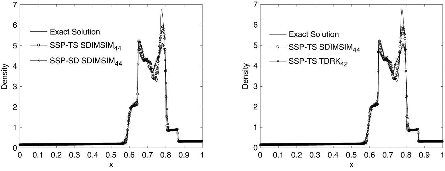
. In Figure 9, the numerical results for the density obtained by the SSP-TS SDIMSIM of order
 $p=4$
together with that for SSP-SD SDIMSIM
 $_{pq}$
with
 $p=q=4$
, and the SSP-TS TDRK
 $_{pq}$
method with order
 $p=4$
and stage order
 $q=2$
have been plotted, using the same temporal stepsize
 $\Delta t$
for all the methods. From this figure, we observe that the proposed method in this work outperforms the two other methods.
 $\Box $
To verify the SSP properties of the proposed schemes in the presence of the shock, we consider the maximal observed rise in total variation over each step defined by
 $$ \begin{align} \max_{1\leq n\leq N_t} (\lVert u(t_n,x)\rVert_{TV}-\lVert u(t_{n-1},x)\rVert_{TV}). \end{align} $$
We are looking for the time-step
 $\Delta t_{\text {obs}}$
, or the SSP coefficient
 $\mathcal {C}^{\text {obs}}=\Delta t_{\text {obs}}/\Delta t_{FE}$
, at which this rise becomes evident and exceeds
 $10^{-10}$
.
Numerical results for Problem 4 obtained by SSP-TS SDIMSIM
 $_{44}$
, SSP-SD SDIMSIM
 $_{44}$
and SSP-TS TDRK
 $_{42}$
.

To show the sharpness of the SSP time-step, we monitor the maximal rise in the total variation. For this, we consider a linear advection problem
 $$ \begin{align*} u_t-u_x=0, \end{align*} $$
and the nonlinear Burgers equation
 $$ \begin{align*} u_t+(\tfrac{1}{2}u^2)_x=0, \end{align*} $$
with
 $x\in [0,1]$
, periodic boundary conditions and the initial condition
 $$ \begin{align} u_0(x)=\left\{\begin{array}{@{}l} 1\quad\text{if } \frac{1}{4}\leq x\leq\frac{1}{2} \\[6pt] 0\quad \text{otherwise}. \end{array} \right. \end{align} $$
As in [Reference Grant, Gottlieb and Seal22], using a first-order spatial discretization results in approximations for the first and second derivatives of the solution which, in the case of the linear advection equation, are given by
 $$ \begin{align*} F(u^n)_j&=\frac{u_{j+1}^n-u_j^n}{\Delta x}\approx u_x(x_j),\\ G(u^n)_j&=\frac{u_{j+2}^n-2u_{j+1}^n+u_j^n}{\Delta x^2}\approx u_{xx}(x_j), \end{align*} $$
and for Burgers equation, are given by
 $$ \begin{align*} F(u^n)_j&=\frac{f_{j}^n-f_{j-1}^n}{\Delta x}\approx f(u)_x(x_j),\\ G(u^n)_j&=\frac{f'(u_j^n)F(u^n)_j-f'(u_{j-1}^n)F(u^n)_{j-1}}{\Delta x}\approx (\,f'(u)f(u)_{x})_x(x_j). \end{align*} $$
To compare the efficiency of the derived time-stepping methods, we use a time-step
 $\Delta t=\lambda \Delta x$
where
 $\lambda $
varies from
 $\lambda =0.05$
until beyond breaching the TVD property (that is,
 $0.05\leq \lambda \leq 3.5$
). For a grid size
 $\Delta x=1/600$
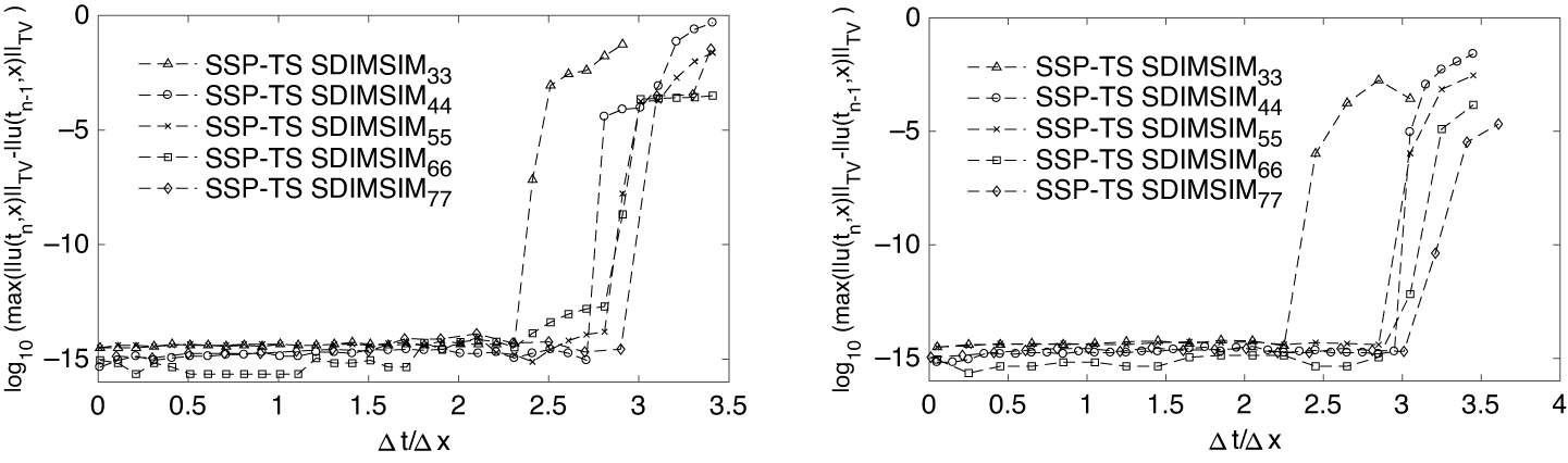
, the maximal rise in total variation (5.1) is plotted in Figure 10 for a selection of time-stepping methods. The point where the maximal rise in total variation exceeds
 $10^{-10}$
is defined as the observed SSP coefficient
 $\mathcal {C}^{\text {obs}}$
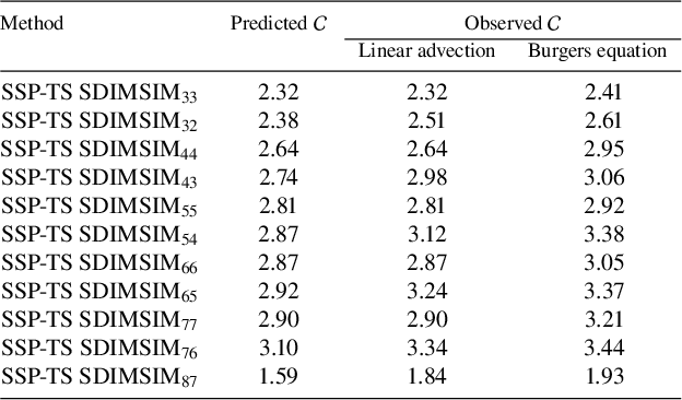
. The expected and observed values of the SSP coefficients are listed in Table 8. The results from the linear advection problem show how well the observed SSP coefficient
 $\mathcal {C}_{TS}^{\text {obs}}$
matches the predicted SSP coefficient
 $\mathcal {C}_{TS}^{\text {pred}}$
for the methods with
 $p=q=r=s$
up to order
 $p=7$
.
Maximal rise in total variation (5.1) as a function of the CFL number for linear advection on the left and for Burgers equation on the right.

Comparison of the observed and theoretical value of SSP coefficients for linear advection and Burgers equation.

6 Conclusions
In this paper, we introduced a formulation based on the forward Euler and Taylor series conditions to extend the SSP framework to SSP SGLMs, which not only increases our flexibility in the choice of spatial discretizations, but also leads to larger SSP coefficients than those of the methods studied by Moradi et al. [Reference Moradi, Abdi and Farzi34] and Ditkowski et al. [Reference Ditkowski, Gottlieb and Grant16]. Within this new pair of base conditions, SSP methods in the class of SDIMSIMs, called “SSP-TS transformed SDIMSIMs,” were studied, and examples of such methods with the abscissa vector
 $-1\leq c\leq 1$
up to order
 $p=8$
were determined. Finally, the proposed methods were examined on some one-dimensional linear and nonlinear problems conforming the capability of derived methods, the verification of theoretical order and potential of such schemes in solving PDEs and sharpness of the SSP time-steps.
Appendix
The coefficient matrices of the constructed SSP-TS SDIMSIMs
-
1. SSP-TS SDIMSIM
$_{33}$
$$ \begin{align*} \tiny{ \begin{array}{l} c=\left[\begin{array}{c} 0.3379637032\\ 0.6709575126\\ 1.0 \end{array}\right],\quad A=\left[\begin{array}{c@{\hspace{2mm}}c@{\hspace{2mm}}c} 0 & 0 & 0\\ 0.3427226266 & 0 & 0\\ 0.2998325752 & 0.3766826971 & 0 \end{array}\right], \\ \\ \overline{A}=\left[\begin{array}{c@{\hspace{2mm}}c@{\hspace{2mm}}c} 0 & 0 & 0\\ 0.0714204330 & 0 & 0\\ 0.0624825171 & 0.0550098602 & 0 \end{array}\right],\\ \\ \widetilde{B}=\left[\begin{array}{c@{\hspace{2mm}}c@{\hspace{2mm}}c} 0.5078023394 & 0.5171810460 & 0.5911620724\\ 0 & 0 & 0\\ 0.0623845271 & 0.0783743124 & 0.0484364010 \end{array}\right],\\ \\ \widetilde{\overline{B}}=\left[\begin{array}{c@{\hspace{2mm}}c@{\hspace{2mm}}c} 0.0857877831 & 0.0755279105 & 0.1058772476\\ 0 & 0 & 0\\ 0.0130003962 & 0.0061883201 & 0 \end{array} \right], \\ \\ \widetilde{U}=\left[\begin{array}{c@{\hspace{2mm}}c@{\hspace{2mm}}c} 0.6264620098 & 0.0000018173 & 0 \\ 0.4986523646 & 2.0452837246 & 1.0403547143\\ 0.4362484732 & 2.2049623004 & 1.5483146767 \end{array} \right], \\ \\ \widetilde{V}=\left[\begin{array}{c@{\hspace{2mm}}c@{\hspace{2mm}}c} 0.7388389843 & 3.4896393266 & 2.1258183881\\ 0 & 0 & 0\\ 0.0907678382 & 0.4287091297 & 0.2611610157 \end{array} \right], \\ \\ \widetilde{W}=\left[\begin{array}{c@{\hspace{2mm}}c@{\hspace{2mm}}c@{\hspace{2mm}}c} 1.5962659897 & 0.5394799651 & 0.0911623234 & 0.0102698521\\ 0 & 0 & 0 & 0\\ 0.1961044507 & 0.0569247439 & -0.0073191934 & 0.0014523797 \end{array}\right].\\[3pt] \end{array}}. \end{align*} $$
-
2. SSP-TS SDIMSIM
$_{44}$
$$ \begin{align*} \tiny{ \begin{array}{l} c=\left[\begin{array}{c} 0.2563967241\\ 0.5101578748\\ 0.7511999445\\ 1.0 \end{array}\right],\quad A=\left[\begin{array}{c@{\hspace{2mm}}c@{\hspace{2mm}}c@{\hspace{2mm}}c} 0 & 0 & 0 & 0\\ 0.2525178632 & 0 & 0 & 0\\ 0.2668995454 & 0.2338475193 & 0 & 0\\ 0.2857735400 & 0.2000149977 & 0.2679177278 & 0 \end{array}\right], \\ \\ \overline{A}=\left[\begin{array}{c@{\hspace{2mm}}c@{\hspace{2mm}}c@{\hspace{2mm}}c} 0 & 0 & 0 & 0\\ 0.0477878826 & 0 & 0 & 0\\ 0.0295253379 & 0.0442546031 & 0 & 0\\ 0.0252536799 & 0.0313259480 & 0.0425708749 & 0 \end{array}\right],\\ \\ \widetilde{B}=\left[\begin{array}{c@{\hspace{2mm}}c@{\hspace{2mm}}c@{\hspace{2mm}}c} 1.4300266680 & 1.2412670239 & 1.0586073420 & 1.4955093362\\ 0.0103995939 & 0.0155876251 & 0 & 0\\ 0.5867713460 & 0.4740495193 & 0.5887015350 & 0.5024992503\\ 0 & 0 & 0 & 0 \end{array}\right], \\ \\ \widetilde{\overline{B}}=\left[\begin{array}{c@{\hspace{2mm}}c@{\hspace{2mm}}c@{\hspace{2mm}}c} 0.1567210483 & 0.1237763504 & 0.1682077594 & 0.2180758207\\ 0.0019680769 & 0.0029498887 & 0 & 0\\ 0.0598529858 & 0.0810475954 & 0.0565187197 & 0\\ 0 & 0 & 0 & 0 \end{array} \right], \\ \\ \widetilde{U}=\left[\begin{array}{c@{\hspace{2mm}}c@{\hspace{2mm}}c@{\hspace{2mm}}c} 0.1935050934 & 0 & 0 & 0 \\ 0.1291007688 & 0 & 0.1569604623 & 0 \\ 0.1364534614 & 0.2418353488 & 0.1328470450 & 0 \\ 0.1461028667 & 0.1711849399 & 0.1083374215 &0.1737668973 \end{array} \right],\\ \\ \widetilde{V}=\left[\begin{array}{c@{\hspace{2mm}}c@{\hspace{2mm}}c@{\hspace{2mm}}c} 0.7311068606 & 0.9167153648 & 0.6150804163 & 1.0393232593\\ 0.0076835780 & 0.0096342332 & 0.0064641964 & 0.0109227826\\ 0.2999892004 & 0.3761484457 & 0.2523810023 & 0.4264571573\\ 0.0048382278 & 0.0060665247 & 0.0040704025 & 0.0068779039 \end{array} \right], \\ \\ \widetilde{W}=\left[\begin{array}{c@{\hspace{2mm}}c@{\hspace{2mm}}c@{\hspace{2mm}}c@{\hspace{2mm}}c} 5.1678226268 & 1.3250127924 & 0.1698644697 & 0.0145175645 & 0.0009305640\\ 0.0543113057 & -0.0150040650 & 0.0046605540 & -0.0017732724 & 0.0005376505\\ 2.1204711117 & 0.5516028698 & -0.0275976540 & -0.0018986858 & 0.0026888288\\ 0.0341989724 & -0.0258115649 & 0.0095153069 & -0.0022732350 & 0.0004141086 \end{array}\right]. \end{array}} \end{align*} $$
-
3. SSP-TS SDIMSIM
$_{55}$
$$ \begin{align*} \tiny{ \begin{array}{l} c=\left[\begin{array}{c} 0.2071288276\\ 0.4062917712\\ 0.6050674218\\ 0.8001048024\\ 1.0 \end{array}\right],\quad A=\left[\begin{array}{c@{\hspace{2mm}}c@{\hspace{2mm}}c@{\hspace{2mm}}c@{\hspace{2mm}}c} 0 & 0 & 0 & 0 & 0\\ 0.1883799083 & 0 & 0 & 0 & 0\\ 0.1972261019 & 0.1876095038 & 0 & 0 & 0\\ 0.2333299954 & 0.1725184495 & 0.1847897127 & 0 & 0\\ 0.2222809919 & 0.1871616858 & 0.1938982318 & 0.1887666939 & 0 \end{array}\right], \\ \\ \overline{A}=\left[\begin{array}{c@{\hspace{2mm}}c@{\hspace{2mm}}c@{\hspace{2mm}}c@{\hspace{2mm}}c} 0 & 0 & 0 & 0 & 0\\ 0.0334265160 & 0 & 0 & 0 & 0\\ 0.0176709306 & 0.0332898139 & 0 & 0 & 0\\ 0.0237493850 & 0.0173341532 & 0.0327894644 & 0 & 0\\ 0.0253846153 & 0.0181885755 & 0.0174410716 & 0.0334951481 & 0 \end{array}\right], \\ \\ \widetilde{B}=\left[\begin{array}{c@{\hspace{2mm}}c@{\hspace{2mm}}c@{\hspace{2mm}}c@{\hspace{2mm}}c} 0.0199882896 & 0.0168116150 & 0.0174202548 & 0.0170613030 & 0.0316862914\\ 0.9938940819 & 0.8651768450 & 0.9441555283 & 0.8605573282 & 0.9098418499\\ 0.4106824934 & 0.3264938007 & 0.3421115086 & 0.4446615367 & 0.4104430174\\ 0.0084589996 & 0.0073634915 & 0.0080356764 & 0 & 0\\ 0.0013320898 & 0 & 0 & 0 & 0 \end{array}\right],\\ \\ \\ \widetilde{\overline{B}}=\left[\begin{array}{c@{\hspace{2mm}}c@{\hspace{2mm}}c@{\hspace{2mm}}c@{\hspace{2mm}}c} 0.0022803529 & 0.0016341027 & 0.0015763766 & 0.0030273925 & 0\\ 0.1093340995 & 0.1009158758 & 0.0795110707 & 0.0858739190 & 0.1614441979\\ 0.0445058894 & 0.0320916852 & 0.0410844388 & 0.0387389857 & 0 \\ 0.0006935669 & 0.0007537846 & 0 & 0 & 0\\ 0 & 0 & 0 & 0 & 0 \end{array} \right], \\ \\ \widetilde{U}=\left[\begin{array}{c@{\hspace{2mm}}c@{\hspace{2mm}}c@{\hspace{2mm}}c@{\hspace{2mm}}c} 0 & 0.2187058469 & 0 & 0 & 0 \\ 0 & 0.1160936449 & 0.2481490615 & 0 & 0.0564414191\\ 1.9405426326 & 0.1215453242 & 0.1311840225 & 0 & 2.9308526650\\ 1.0104491208 & 0.1437952162 & 0.1206317575 & 0.1846489453 & 2.3667973789\\ 1.0602554386 & 0.1369860022 & 0.1308708903 & 0.3837857224 & 2.2786380119 \end{array} \right], \\ \\ \widetilde{V}=\left[\begin{array}{c@{\hspace{2mm}}c@{\hspace{2mm}}c@{\hspace{2mm}}c@{\hspace{2mm}}c} 0.1038282964 & 0.0123182637 & 0.0121665242 & 0.0465426658 & 0.2099011718\\ 5.1627393621 & 0.6125111093 & 0.6049660406 & 2.3142790627 & 10.4370877592\\ 2.1332722598 & 0.2530929545 & 0.2499752906 & 0.9562728194 & 4.3126619859\\ 0.0439399038 & 0.0052130618 & 0.0051488459 & 0.0196967525 & 0.0888297083\\ 0.0069194822 & 0.0008209323 & 0.0008108199 & 0.0031017667 & 0.0139885511 \end{array} \right], \\ \\ \widetilde{W}=\left[\begin{array}{c@{\hspace{2mm}}c@{\hspace{2mm}}c@{\hspace{2mm}}c@{\hspace{2mm}}c@{\hspace{2mm}}c} 0.0919549546 & 0.0300336963 & 0.0007068533 & -0.0001754669 & 0.0000241295 & 0.0000011638\\ 4.5723514669 & 0.9470657989 & 0.0980823143 & 0.0067718916 & 0.0003506635 & 0.0000145265\\ 1.8893207389 & 0.4358779150 & -0.0054101573 & -0.0022955672 & 0.0004031667 & 0.0001048145\\ 0.0389151319 & -0.0070073631 & -0.0008248687 & 0.0005749511 & -0.0001476518 & 0.0000309087\\ 0.0061282011 & -0.0035284919 & 0.0008303862 & -0.0000554406 & -0.0000250663 & 0.0000107950 \end{array}\right]. \end{array}} \end{align*} $$
-
4. SSP-TS SDIMSIM
$_{66}$
$$ \begin{align*} \tiny{ \begin{array}{l} c=\left[\begin{array}{c} 0.1758227027\\ 0.3489954910\\ 0.5056750884\\ 0.6663037517\\ 0.8309580239\\ 1.0 \end{array}\right],\quad A=\left[\begin{array}{c@{\hspace{2mm}}c@{\hspace{2mm}}c@{\hspace{2mm}}c@{\hspace{2mm}}c@{\hspace{2mm}}c} 0 & 0 & 0 & 0 & 0 & 0\\ 0.1592079838 & 0 & 0 & 0 & 0 & 0\\ 0.2084081661 & 0.1340733423 & 0 & 0 & 0 & 0\\ 0.2509084613 & 0.1034469341 & 0.1432983441 & 0 & 0 & 0\\ 0.2158757433 & 0.1523459345 & 0.1518063268 & 0.1455326667 & 0 & 0\\ 0.2118839745 & 0.1379137715 & 0.2392257619 & 0.0915280170 & 0.1552925550 & 0 \end{array}\right], \\ \\ \overline{A}=\left[\begin{array}{c@{\hspace{2mm}}c@{\hspace{2mm}}c@{\hspace{2mm}}c@{\hspace{2mm}}c@{\hspace{2mm}}c} 0 & 0 & 0 & 0 & 0 & 0\\ 0.0276520711 & 0 & 0 & 0 & 0 & 0\\ 0.0106727733 & 0.0232865558 & 0 & 0 & 0 & 0\\ 0.0245531489 & 0.0096062440 & 0.0248888021 & 0 & 0 & 0\\ 0.0227801279 & 0.0136484077 & 0.0104272951 & 0.0252768708 & 0 & 0\\ 0.0169841860 & 0.0175889806 & 0.0219388943 & 0.0113000698 & 0.0269720190 & 0 \end{array}\right],\\ \\ \widetilde{B}=\left[\begin{array}{c@{\hspace{2mm}}c@{\hspace{2mm}}c@{\hspace{2mm}}c@{\hspace{2mm}}c@{\hspace{2mm}}c} 0.0253287298 & 0.0208649616& 0.0092156832& 0.0223397949& 0 & 0\\ 0.0015900854 & 0.0015111152& 0 & 0 & 0 & 0\\ 0 & 0 & 0 & 0 & 0 & 0\\ 0.0708493417 & 0.0461330727& 0.0609357918& 0.0368303909& 0.0780142252& 0.0544130018\\ 0.5303165780 & 0.3244119948& 0.5161928905& 0.3269585521& 0.3770303108& 0.4248714447\\ 0.0099525856 & 0.0070236513& 0.0069987736& 0.0067095371& 0.0160149244& 0 \end{array}\right],\\ \\ \widetilde{\overline{B}}=\left[\begin{array}{c@{\hspace{2mm}}c@{\hspace{2mm}}c@{\hspace{2mm}}c@{\hspace{2mm}}c@{\hspace{2mm}}c} 0.0031756454 & 0.0006177887 & 0.0016006278 & 0 & 0 & 0\\ 0.0002761743 & 0.0002624584 & 0 & 0 & 0 & 0\\ 0 & 0 & 0 & 0 & 0 & 0\\ 0.0062595955 & 0.0048646511 & 0.0050481848 &0.0056768091 &0.0135499166 & 0\\ 0.0453259218 & 0.0383721079 & 0.0570838733 &0.0274351133 &0.0329896861 & 0.0737938834\\ 0.0010502392 & 0.0006292368 & 0.0004807328 &0.0011653473 & 0 & 0\\ \end{array} \right], \\ \\ \widetilde{U}=\left[\begin{array}{c@{\hspace{2mm}}c@{\hspace{2mm}}c@{\hspace{2mm}}c@{\hspace{2mm}}c@{\hspace{2mm}}c} 0 & 0 &0.3433475631 & 0 & 0.3767676119 & 1.4929992899\\ 0 & 0 &1.4884820475 & 1.1059395619 & 0.1726814104 & 4.4947525319\\ 0.5220851455 & 0.3232476256 &1.2088204677 & 0.8115763837 & 0.2260452975 & 2.3664551849\\ 0.3062804078 & 0.1333471376 &0.9281505742 & 0.4880551153 & 0.2721423006 & 2.7928048845\\ 0.4174497978 & 0.2898936624 &1.4672402894 & 0.6531599584 & 0.2341448396 & 3.3342131647\\ 0.4510968767 & 0.4180592956 &1.3398043652 & 0.7040306450 & 0.2298152560 & 3.0966732050 \end{array} \right], \end{array}} \end{align*} $$
$$ \begin{align*} \tiny{ \begin{array}{l} \widetilde{V}=\left[\begin{array}{c@{\hspace{2mm}}c@{\hspace{2mm}}c@{\hspace{2mm}}c@{\hspace{2mm}}c@{\hspace{2mm}}c} 0.0489794405 & 0.0656246453 & 0.1809629881 & 0.0766353452 & 0.0274722453 & 0.4004228929\\ 0.0030748282 & 0.0041197799 & 0.0113604831 & 0.0048110089 & 0.0017246509 & 0.0251377232\\ 0 & 0 & 0 & 0 & 0 & 0\\ 0.1370049405 & 0.1835647882 & 0.5061883752 & 0.2143638390 & 0.0768451680 & 1.1200600502\\ 1.0254998773 & 1.3740064196 & 3.7888861129 & 1.6045413382 & 0.5751961206 & 8.3837957924\\ 0.0192458160 & 0.0257863266 & 0.0711069857 & 0.0301128339 & 0.0107948513 & 0.1573408199 \end{array} \right], \\ \\ \widetilde{W}=\left[\begin{array}{c@{\hspace{2mm}}c@{\hspace{2mm}}c@{\hspace{2mm}}c@{\hspace{2mm}}c@{\hspace{2mm}}c@{\hspace{2mm}}c} 0.1179917209 & -0.0208608047 & -0.0004845339 & 0.0006754460 & -0.0001064733 & -0.0000006808 & 0.0000048639\\ 0.0074072768 & -0.0030893301 & 0.0007925466 & -0.0002229686 & 0.0000656030 & -0.0000161301 & 0.0000032006\\ 0 & 0 & 0 & 0 & 0 & 0 & 0\\ 0.3300455972 & 0.0713447101 & 0.0049125944 & -0.0010676069 & 0.0000059684 & 0.0000264151 & -0.0000044759\\ 2.4704344098 & 0.4351498499 & 0.0485776109 & 0.0018560110 & 0.0000831963 & 0.0000225399 & -0.0000062521\\ 0.0463632685 & 0.0079520017 & -0.0019060016 & 0.0001383800 & 0.0000056752 & -0.0000047502 & 0.0000016052 \end{array}\right]. \end{array}} \end{align*} $$
-
5. SSP-TS SDIMSIM
$_{77}$
$$ \begin{align*} \tiny{ \begin{array}{l} c=\left[\begin{array}{c} 0.1515413917\\ 0.3001733973\\ 0.4407591855\\ 0.5793400232\\ 0.7165512545\\ 0.8569705290\\ 1.0 \end{array}\right],\quad A=\left[\begin{array}{c@{\hspace{2mm}}c@{\hspace{2mm}}c@{\hspace{2mm}}c@{\hspace{2mm}}c@{\hspace{2mm}}c@{\hspace{2mm}}c} 0 & 0 & 0 & 0 & 0 & 0 & 0\\ 0.1301340685 & 0 & 0 & 0 & 0 & 0 & 0\\ 0.1030782912 & 0.1181748638 & 0 & 0 & 0 & 0 & 0\\ 0.2107058095 & 0.0746962299 & 0.1165405952 & 0 & 0 & 0 & 0\\ 0.1674186626 & 0.1106597053 & 0.1441631890 & 0.1111538975 & 0 & 0 & 0\\ 0.1498499141 & 0.1005976520 & 0.1658168192 & 0.1427112759 & 0.1148778197 & 0 & 0\\ 0.1664059921 & 0.1002871522 & 0.1450512108 & 0.1765674393 & 0.1097236911 & 0.1198084819 & 0 \end{array}\right], \\ \\ \overline{A}=\left[\begin{array}{c@{\hspace{2mm}}c@{\hspace{2mm}}c@{\hspace{2mm}}c@{\hspace{2mm}}c@{\hspace{2mm}}c@{\hspace{2mm}}c} 0 & 0 & 0 & 0 & 0 & 0 & 0\\ 0.0223925474 & 0 & 0 & 0 & 0 & 0 & 0\\ 0.0076892879 & 0.0203346923 & 0 & 0 & 0 & 0 & 0\\ 0.0258115660 & 0.0068860843 & 0.0200534789 & 0 & 0 & 0 & 0\\ 0.0223245458 & 0.0135846477 & 0.0064769707 & 0.0191265742 & 0 & 0 & 0\\ 0.0180234432 & 0.0136574714 & 0.0092710458 & 0.0063845587 & 0.0197673603 & 0 & 0\\ 0.0199392106 & 0.0109409792 & 0.0145398574 & 0.0150938539 & 0.0068816686 & 0.0206157937 & 0 \end{array}\right], \\ \\ \widetilde{B}=\left[\begin{array}{c@{\hspace{2mm}}c@{\hspace{2mm}}c@{\hspace{2mm}}c@{\hspace{2mm}}c@{\hspace{2mm}}c@{\hspace{2mm}}c} 0.0016808588 & 0.0009633972 & 0.0028055808 & 0 & 0 & 0 & 0\\ 0.9547389339 & 0.6449471638 & 0.9755230081 & 0.9547556799 & 0.6499302492 & 1.8501845350 & 0.1595505247\\ 0.4645330948 & 0.2815074221 & 0.3667369941 & 0.2827645985 & 0.8754731480 & 0 & 0\\ 0.4492585157 & 0.2801464628 & 0.3906618309 & 0.4531760282 & 0.3637148863 & 0.3001903692 & 0.8032351738\\ 0.0216469592 & 0.0118916309 & 0.0171995657 & 0.0209366282 & 0.0130105762 & 0.0142063885 & 0.0408073705\\ 0.0702636996 & 0.0459940643 & 0.0766932256 & 0.0642605071 & 0.0517275660 & 0.1549631189 & 0\\ 0.0001908713 & 0.0000221049 & 0.0000643733 & 0 & 0 & 0 & 0 \end{array}\right],\\ \\ \\ \widetilde{\overline{B}}=\left[\begin{array}{c@{\hspace{2mm}}c@{\hspace{2mm}}c@{\hspace{2mm}}c@{\hspace{2mm}}c@{\hspace{2mm}}c@{\hspace{2mm}}c} 0.0000626854 & 0.0001657746 & 0.0004827644 & 0 & 0 & 0 & 0\\ 0.1158725224 & 0.0788678955 & 0.0625860535 & 0.0402916863 & 0.1062725827 & 0.2129554731 & 0\\ 0.0567914519 & 0.0345580097 & 0.0164767773 & 0.0486561263 & 0.0838836601 & 0 & 0\\ 0.0546497809 & 0.0303293144 & 0.0363860961 & 0.0412102044 & 0.0172426076 & 0.0481171934 & 0.1382150108\\ 0.0023643082 & 0.0012973355 & 0.0017240755 & 0.0017897660 & 0.0008159995 & 0.0024445346 & 0\\ 0.0081609828 & 0.0062696009 & 0.0045236778 & 0.0028748603 & 0.0089009126 & 0 & 0\\ 0.0000014383 & 0.0000038037 & 0 & 0 & 0 & 0 & 0 \end{array} \right],\\ \\ \widetilde{U}=\left[\begin{array}{c@{\hspace{2mm}}c@{\hspace{2mm}}c@{\hspace{2mm}}c@{\hspace{2mm}}c@{\hspace{2mm}}c@{\hspace{2mm}}c} 0 & 0 & 0.2035629971 & 0.1668794884 & 0 & 0 & 0\\ 0 & 0.1004101687 & 0.0769745847 & 0.0631032138 & 0 & 0 & 0\\ 0 & 0.0362873794 & 0.0609710336 & 0.1952183393 & 0 & 0.1746634164 & 0\\ 0.0550884948 & 0.0224060792 & 0.1246329449 & 0.1513550849 & 0 & 0.2442797764 & 0\\ 0.2097640029 & 0.0330441233 & 0.0990285032 & 0.1420218979 & 0 & 0.2993334461 & 0.1980273583\\ 0.2071785413 & 0.0302221096 & 0.1012240870 & 0.1426408077 & 0.0958024529 & 0.2933574084 & 0.0661026528\\ 0.1979697114 & 0.0303936303 & 0.1028116422 & 0.1419056033 & 0.1040177729 & 0.2835063842 & 0.3534698372 \end{array} \right], \\ \\ \widetilde{V}=\left[\begin{array}{c@{\hspace{2mm}}c@{\hspace{2mm}}c@{\hspace{2mm}}c@{\hspace{2mm}}c@{\hspace{2mm}}c@{\hspace{2mm}}c} 0.0028070189 & 0.0004421897 & 0.0014453966 & 0.0019990614 & 0.0012980075 & 0.0040056188 & 0.0099541767\\ 1.2281519380 & 0.1934707746 & 0.6324028261 & 0.8746471611 & 0.5679158053 & 1.7525740687 & 4.3552401738\\ 0.5336190219 & 0.0840610044 & 0.2747723364 & 0.3800249368 & 0.2467534083 & 0.7614748888 & 1.8923057725\\ 0.5373960345 & 0.0846559972 & 0.2767172045 & 0.3827147940 & 0.2484999553 & 0.7668646896 & 1.9056997155\\ 0.0266729970 & 0.0042017972 & 0.0137345211 & 0.0189955822 & 0.0123339923 & 0.0380623939 & 0.0945870819\\ 0.0932890413 & 0.0146958227 & 0.0480366081 & 0.0664372157 & 0.0431382465 & 0.1331235572 & 0.3308191503\\ 0.0002192579 & 0.0000345397 & 0.0001129008 & 0.0001561479 & 0.0001013881 & 0.0003128812 & 0.0007775266 \end{array} \right], \\ \\ \widetilde{W}=\left[\begin{array}{c@{\hspace{2mm}}c@{\hspace{2mm}}c@{\hspace{2mm}}c@{\hspace{2mm}}c@{\hspace{2mm}}c@{\hspace{2mm}}c@{\hspace{2mm}}c} 0.0141550255 & -0.0061308267 & 0.0016738474 & -0.0003561799 & 0.0000520541 & -0.0000030001 & -0.0000007566 & 0.0000002843\\ 6.1932330112 & 1.1227548920 & -0.0139739183 & -0.0059672033 & -0.0000261796 & 0.0000419185 & 0.0000042917 & 0.0000002622\\ 2.6908942124 & 0.0695115947 & -0.0424262678 & 0.0003622426 & 0.0003394668 & -0.0000000600 & -0.0000025912 & -0.0000000346\\ 2.7099406499 & 0.8232971254 & 0.1205589442 & 0.0030338077 & -0.0002824113 & 0.0000040641 & 0.0000032616 & 0.0000000444\\ 0.1345046001 & 0.0296567518 & 0.0036158510 & -0.0006691561 & 0.0000572187 & 0.0000066989 & -0.0000036626 & 0.0000008602\\ 0.4704310212 & 0.0790280340 & -0.0138820999 & 0.0005516865 & 0.0000629185 & -0.0000117776 & 0.0000001838 & 0.0000004879\\ 0.0011056574 & -0.0006272230 & 0.0001536316 & -0.0000131713 & -0.0000038323 & 0.0000018639 & -0.0000004523 & 0.0000000805 \end{array}\right]. \end{array}} \end{align*} $$
-
6. SSP-TS SDIMSIM
$_{87}$
$$ \begin{align*} \tiny{ \hspace{-1cm}\begin{array}{l} \hspace{-1cm} c=\left[\begin{array}{c} 0.2311609775\\ -0.1464553791\\ 0.4861919221\\ -0.8479793337\\ 0.7360212915\\ 0.7035168041\\ 0.3386114110\\ 1.0 \end{array}\right],\quad A=\left[\begin{array}{c@{\hspace{2mm}}c@{\hspace{2mm}}c@{\hspace{2mm}}c@{\hspace{2mm}}c@{\hspace{2mm}}c@{\hspace{2mm}}c@{\hspace{2mm}}c} 0 & 0 & 0 & 0 & 0 & 0 & 0 & 0\\ 0.0002812522 & 0 & 0 & 0 & 0 & 0 & 0 & 0\\ 0.2153483369 & 0.2395600879 & 0 & 0 & 0 & 0 & 0 & 0\\ 0.0000021930 & 0.0000024396 & 0.0000064453 & 0 & 0 & 0 & 0 & 0\\ 0.2660875910 & 0.2450226058 & 0.2028620170 & 0.0257466856 & 0 & 0 & 0 & 0\\ 0.3228294275 & 0.2416355368 & 0.0779653887 & 0.0078930145 & 0.0210518147 & 0 & 0 & 0\\ 0.1778073516 & 0.1582203440 & 0.0003948087 & 0.0979412549 & 0.0012286718 & 0 & 0 & 0\\ 0.2609726524 & 0.1532765453 & 0.0727791374 & 0.0753707410 & 0.2270648817 & 0 & 0.2622939542 & 0 \end{array}\right],\\ \\ \hspace{-1cm} \overline{A}=\left[\begin{array}{c@{\hspace{2mm}}c@{\hspace{2mm}}c@{\hspace{2mm}}c@{\hspace{2mm}}c@{\hspace{2mm}}c@{\hspace{2mm}}c@{\hspace{2mm}}c} 0 & 0 & 0 & 0 & 0 & 0 & 0 & 0\\ 0.0000890049 & 0 & 0 & 0 & 0 & 0 & 0 & 0\\ 0.0681489787 & 0 & 0 & 0 & 0 & 0 & 0 & 0\\ 0.0000006940 & 0 & 0.0000020397 & 0 & 0 & 0 & 0 & 0\\ 0.0218666578 & 0.0438643230 & 0.0641975669 & 0 & 0 & 0 & 0 & 0\\ 0.1000888710 & 0.0014589928 & 0.0145440149 & 0.0018955680 & 0.0066620420 & 0 & 0 & 0\\ 0.0000647396 & 0.0458496693 & 0.0001249409 & 0.0228418607 & 0.0003888246 & 0 & 0 & 0\\ 0.0369805761 & 0.0347024167 & 0.0230316331 & 0.0127438942 & 0.0718567880 & 0 & 0 & 0 \end{array}\right], \\ \\ \hspace{-1cm} \widetilde{B}=\left[\begin{array}{c@{\hspace{2mm}}c@{\hspace{2mm}}c@{\hspace{2mm}}c@{\hspace{2mm}}c@{\hspace{2mm}}c@{\hspace{2mm}}c@{\hspace{2mm}}c} 0.0779083031 & 0.0912873356 & 0.0275723752 & 0.0076540512 & 0.0600247478 & 0 & 0 & 0\\ 0 & 0 & 0 & 0 & 0 & 0 & 0 & 0\\ 0.6165809624 & 0.7303530449 & 0.2182129629 & 0.0340897896 & 0.4750471427 & 0.5861161339 & 0 & 0\\ 2.2258588756 & 2.1225710982 & 0.7877493630 & 0.3001599573 & 0.6795001122 & 2.6900132377 & 0.9839905195 & 1.6429936281\\ 0.0620841130 & 0.0103342292 & 0.0049071024 & 0.0265015170 & 0.0153090727 & 0 & 0.0176842724 & 0.0426723676\\ 0.0030518919 & 0.0000000057 & 0.0000000150 & 0.0014688078 & 0 & 0 & 0 & 0\\ 1.5645493937 & 1.3226762697 & 0.5537066172 & 0.3206052718 & 1.1952363050 & 1.1830434130 & 1.6424119796 & 0.0161482825\\ 0.0005973276 & 1.3405598827 & 0.0000047591 & 0.4673341037 & 0 & 0 & 0 & 0 \end{array}\right],\\ \\ \hspace{-1cm} \widetilde{\overline{B}}=\left[\begin{array}{c@{\hspace{2mm}}c@{\hspace{2mm}}c@{\hspace{2mm}}c@{\hspace{2mm}}c@{\hspace{2mm}}c@{\hspace{2mm}}c@{\hspace{2mm}}c} 0.0029802024 & 0.0246968519 & 0.0060883875 & 0 & 0 & 0 & 0 & 0\\ 0 & 0 & 0 & 0 & 0 & 0 & 0 & 0\\ 0.1084728837 & 0.0329230693 & 0.0596756589 & 0.0043658374 & 0.1503330746 & 0.1854818871 & 0 & 0\\ 0.5502748346 & 0.1182421696 & 0.2062412058 & 0.0596895774 & 0.2150341132 & 0 & 0.0959192792 & 0.5199405732\\ 0.0165722218 & 0.0023396917 & 0.0015528981 & 0.0068010081 & 0.0048446981 & 0 & 0 & 0\\ 0.0009657995 & 0 & 0.0000000047 & 0 & 0 & 0 & 0 & 0\\ 0.2318571018 & 0.2015937455 & 0.1444290593 & 0.0637296896 & 0.0152908407 & 0.0188214018 & 0 & 0\\ 0.0001890299 & 0.1818670655 & 0.0000015061 & 0.0935808935 & 0 & 0 & 0 & 0 \end{array} \right], \\ \\ \hspace{-1cm} \widetilde{U}=\left[\begin{array}{c@{\hspace{2mm}}c@{\hspace{2mm}}c@{\hspace{2mm}}c@{\hspace{2mm}}c@{\hspace{2mm}}c@{\hspace{2mm}}c@{\hspace{2mm}}c} 0 & 0.0091736086 & 0 & 0.1104479186 & 0 & 0 & 0 & 0\\ 0 & 0.0004744032 & 0 & 0.0000490801 & 0 & 0 & 0.1056970619& 0.03318154915\\ 0 & 0.1147325272 & 0.1122074193 & 0.0375795204 & 0 & 0 & 0.0400064074& 0.0125592382\\ 0 & 0.0017139035 & 0.0000011427 & 0.0000003827 & 0 & 0 & 0.0000004074& 0.1015048077\\ 0.1948458836& 0.3369733217 & 0.0359645382 & 0.0464338113 & 0& 0& 0.0409186450& 0.0169747572\\ 0.0064808646& 0.3640663649 & 0.0138221499 & 0.0563355874 & 0.2254137439& 0.1779184837& 0.0403530063& 0.0139338929\\ 0.0003782503& 1.4015034834 & 0.0000699939 & 0.0310284031 & 0.3529749718& 0.8403921765& 0.0601405205& 0.0240022856\\ 0.1926952813& 1.0272027602 & 0.0129027016 & 0.0455412252 & 0.1462798032& 0.5818706839& 0.0395704272& 0.0201233415 \end{array} \right], \\ \\ \hspace{-1cm} \widetilde{V}=\left[\begin{array}{c@{\hspace{2mm}}c@{\hspace{2mm}}c@{\hspace{2mm}}c@{\hspace{2mm}}c@{\hspace{2mm}}c@{\hspace{2mm}}c@{\hspace{2mm}}c} 0.0184787995 & 0.2705727866 & 0.0048881883 & 0.0135954459 & 0.0665923957 & 0.1254523185& 0.0154113814& 0.0060133760\\ 0 & 0 & 0 & 0 & 0 & 0 & 0 & 0\\ 0.1462446947 & 2.1413639183 & 0.0386860417 & 0.1075969157 & 0.5270247436 & 0.9928532416& 0.1219685706& 0.0475909886\\ 0.5279437278 & 7.7303293068 & 0.1396567108 & 0.3884251450 & 1.9025606930 & 3.5842027811& 0.4403068566& 0.1718035924\\ 0.0147255149 & 0.2156159331 & 0.0038953337 & 0.0108340339 & 0.0530666137 & 0.0999713203& 0.0122811293& 0.0047919811\\ 0.0007238676 & 0.0105991129 & 0.0001914844 & 0.0005325726 & 0.0026086153 & 0.0049143275& 0.0006037081& 0.0002355612\\ 0.3710900310 & 5.4336248191 & 0.0981642748 & 0.2730228461 & 1.3373040903 & 2.5193251691& 0.3094903424& 0.1207602195\\ 0.5744532388 & 8.4113371806 & 0.1519598503 & 0.4226436849 & 2.0701678881 & 3.8999552178& 0.4790959463& 0.1869387302 \end{array} \right], \\ \\ \hspace{-1cm} \widetilde{W}=\left[\begin{array}{c@{\hspace{2mm}}c@{\hspace{2mm}}c@{\hspace{2mm}}c@{\hspace{2mm}}c@{\hspace{2mm}}c@{\hspace{2mm}}c@{\hspace{2mm}}c@{\hspace{2mm}}c} 0.3169046293& -0.0624631453& 0.0073573488 &-0.0058606830& 0.0047136483&-0.0019803415& 0.0004655098&-0.0000319171& 0.1045502478\\ 0 & 0 & 0 & 0 & 0 & 0 & 0 & 0 & 0\\ 2.5080428352 & 0.0731731474 & 0.1983823136 &-0.0482405607& 0.0012735643& 0.0004839542& 0.0000812276& 0.0000075604& 0.8275668281\\ 9.0540411491 & 2.0929410020 & 0.2419031439 & 0.0186395224& 0.0010771826& 0.0000498005& 0.0000019187& 0.0000000634& 2.9876705936\\ 0.2525371757 &-0.0810176178 & 0.0505730911 &-0.0135538343& 0.0017501218& 0.0001143595&-0.0000216526&-0.0000581930& 0.0833743771\\ 0.0124140642 &-0.0082852813 & 0.0030464367 &-0.0002292075&-0.0005315179& 0.0004135018&-0.0001903133& 0.0000662444& 0.0040774981\\ 6.3640578232 & 1.2333933570 &-1.0120420107 & 0.3090839217&-0.0664770940& 0.0112931616&-0.0015970467& 0.0001934641& 2.1000264167\\ 9.8516621905 &-8.3542032894 & 3.5419854417 &-1.0012137725& 0.2122442526&-0.0359969521& 0.0050873037&-0.0006162890& 3.2509682925 \end{array}\right]. \end{array}} \end{align*} $$