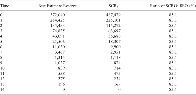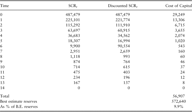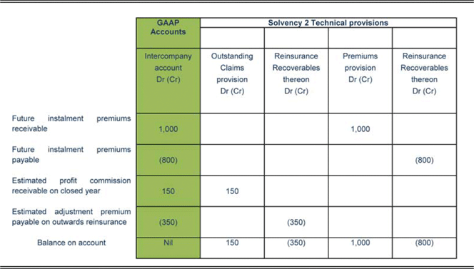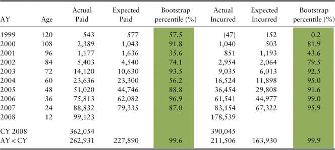


1. Introduction
1.1. Background
The Solvency II requirements for technical provisions are challenging when compared with current requirements for IFRS/GAAP and earlier solvency regimes. To make things more interesting, at the time of writing, some of the requirements are well articulated and final, while there remains significant ambiguity in others, and the requirements (many still in draft) are spread across several sections of the Level 1 Solvency II Directive, European Commission Draft Implementing measures, EIOPA Solvency II Final L2 Advice and the EIOPA Long Term Guarantees Technical Specifications. (At the time of writing, the final Level 2 and Level 3 advice has not been published.)
As far as we are aware, there is only one publically available, authoritative and logically ordered guide to calculating Solvency II technical provisions and that is the Detailed Technical Provisions Guidance issued by Lloyd’s of London in 2010, updated March 2011, and we recommend this to our readers.
The aim of this paper is threefold: to help individuals new to the Solvency II requirements to climb what may be a steep learning curve more quickly than we, its authors, were able to; to fuel debate amongst more experienced practitioners as to how to deal with some of the more ambiguous areas; and, hopefully, to promote best practice. In particular, we hope to push forward the debate on how to deal with some of the more contentious issues, in order to help the industry to reach a consensus on how to approach these issues in ways that are practical and acceptable to the supervisory authorities.
In the paper, we have tried to explain the Solvency II requirements and to suggest how they may be implemented. Where we have used words like “should”, we think it is the right thing to do, but we accept that others may have different views. It is not our intention to give advice, or to be seen to give advice, but rather to make suggestions and observations that we hope the reader will find useful and interesting.
Different sections of the paper have been written by different members of the working party. To make the paper interesting and to fuel debate individuals have in places very much given their own interpretation of the guidelines and how they should be applied. We do not necessarily all agree on these points. Indeed, if we had had to ensure everyone’s full agreement to every point raised the paper might never have been completed. We reiterate that it is not our intention to give advice, but rather to fuel the debate. It is the responsibility of the actuary/reserving specialist in each EC (re)insurance entity to ensure that they meet the Solvency II requirements relating to technical provisions. We do not think it is appropriate to rely on this paper for that purpose, but we would be delighted if you find it useful in informing your thinking in this area.
1.2. Why are Technical Provisions Important?
Technical provisions are normally the largest item on a general insurer’s balance sheet. This is no different under Solvency II and confirms that the calculation of technical provisions will remain an essential component in the construction of solvency balance sheets.
Solvency II intends the balance sheet to be a tool for management to assess their solvency and hence a key consideration for significant decisions. It will also be a tool for regulators to assess the solvency of the insurer.
A key consideration for management in making significant decisions will be the excess of the value of assets over technical provisions, other liabilities (such as outstanding tax payments) and the solvency capital requirement (SCR). This excess of “own funds”, to use Solvency II terminology, over the SCR will determine whether the (re)insurer can expand existing business, move into new areas, consider mergers/acquisitions with less capital rich entities, etc., or whether they need to consider reducing the volume of business they write, moving out of more volatile, capital-intensive types of risk, purchasing additional reinsurance and so on. The level of own funds will also often impact an insurer’s credit rating.
Simplified Illustration of a Solvency II Balance Sheet

The technical provisions are a direct input into the balance sheet. They are therefore also a key input into the SCR calculation that models the potential movement in the Solvency II balance sheet over a 1-year time horizon. Thus, if we get our technical provisions wrong, there is a potential “double whammy” as the capital could equally be wrong. This would amplify the potential impact on the excess of own funds over the SCR. The consequence are that management and regulators could be significantly misinformed and the ramifications for the (re)insurer severe.
1.3. Scope
1.3.1. Deterministic approach
We have assumed throughout this paper that the (re)insurer has chosen to use a deterministic approach for estimating its Solvency II technical provisions, rather than a stochastic approach. A stochastic approach would be equally valid, but at the time of writing, very few (re)insurers were using a stochastic approach. Most insurers are choosing to adapt existing reserve estimates for IFRS/GAAP accounts and/or actuarial opinions rather than calculate the Solvency II technical provisions from scratch. This may change over time, and it is not the purpose of this paper to advocate one approach over the other, but our experience is based on converting existing reserve estimates and so this is the approach that we have assumed here.
1.3.2. Expert judgement and proportionality
The Solvency II Directive and draft guidance makes frequent reference to proportionality and the application of expert judgement. How one determines what is proportional and where and how to ensure expert judgement is appropriate is important to the calculation of technical provisions, but not specific to technical provisions alone. In order to keep our scope manageable (given that each of these subjects could generate a paper on its own), we have decided not to try to cover either of these issues in-depth in this paper.
1.4. Who We are: the Profession’s GI ROC Solvency II Technical Provisions Working Party
The Institute and Faculty of Actuaries General Insurance Reserving Oversight Committee’s Working Party on Solvency II Technical Provisions for General Insurers was established in 2009 for the purpose of providing education to the wider actuarial community on the Solvency II requirements and informing the debate in the wider reserving community as to how the requirements should be implemented for general insurance undertakings.
Membership of the working party has changed over the time it has been in existence. This paper is mostly the work of it current members, but we should credit former members both for helping us to form our ideas and in some cases for contributing to early drafts of the paper parts of which were first drafted back in 2010. We shall not list everyone who has helped (partly for fear that we will forget someone), but you know who you are and we are grateful for the help you have given.
Since its establishment, the working party has presented at numerous events and hosted a sessional round table meeting at Staple Inn. This is the first paper that the working party has published.
2. Solvency II Requirements for Technical Provisions in Brief
2.1. The Basic Requirements
Under Solvency II, the technical provisions are made up of:
 $${Claims}\;{provision}\,{\rm {\plus}}\,{Premium}\;{provision}\,{\rm {\plus}}\,{Risk}\;{margin}$$
The claims provision is the discounted best estimate of all future cash flows (claim payments, expenses and future premiums) relating to claim events before the valuation date.
The premium provision is the discounted best estimate of all future cash flows (claim payments, expenses and future premiums due) relating to future exposure arising from policies that the (re)insurer is obligated to at the valuation date.
The risk margin is intended to be the balance that another (re)insurer taking on the liabilities at the valuation date would require over and above the best estimate. It is calculated using a cost of capital approach.
In normal circumstances, the valuation of the best estimate for claims provisions and for premium provisions should be carried out separately. Claims and premium provisions should be calculated gross of outwards reinsurance and for reinsurance. The risk margin need only be calculated net of reinsurance.
The discount rates to be used will be provided by EIOPA for all major currencies.
2.2. Data
The Solvency II Directive requires that insurance and reinsurance undertakings have internal processes and procedures in place to ensure the appropriateness, completeness and accuracy of the data used in the calculation of their technical provisions.
The EC Draft Level 2 guidance gives the following minimal criteria that must be met for data to be considered appropriate, complete and accurate.
2.2.1. Appropriateness of data
For data to be considered appropriate, at least:
∙ the data are suitable for the purposes of calculating technical provisions;
∙ there is no undue estimation error arising from the amount or nature of the data;
∙ the data are consistent with the methods and assumptions used to calculate the provisions; and
∙ the data appropriately reflect the underlying risks.
2.2.2. Completeness of data
For data to be considered complete, at least:
∙ the data are of sufficient granularity and include sufficient information to identify trends and assess the characteristics of the underlying risk;
∙ there are data available for each homogeneous risk group in the calculation; and
∙ no relevant data are excluded from use in the calculation without justification.
2.2.3. Accuracy of data
For data to be considered accurate, at least:
∙ the data are free from material errors;
∙ data from different time periods used for the same estimation are consistent; and
∙ the recording of the data is consistent over time, and performed in a timely manner.
3. Best Estimate: Claims and Premium Provision
3.1. Introduction
Solvency II requires the technical provisions to be a “best estimate” of the current liabilities relating to insurance contracts plus a risk margin. This section covers the claims provision and the premium provision that together make up the best estimate.
We cover the guidance and the basic requirements for a gross best estimate. We do not discuss reinsurance or ENID (Events Not in Data) in any detail because both of these issues are sufficiently complex to warrant their own sections in the paper – see sections 4 and 6. At the end of this section, we discuss the practical issues that arise in calculating the best estimate and suggest possible approaches.
It could be said that, apart from ENID, there are relatively few “new” issues in the calculation of the claims provision. The theory of producing a discounted best estimate is relatively straight forward, albeit projecting the timing of some future cash flows may be tricky. Calculating the premium provision is more challenging and so gets more attention here.
3.1.1. The guidance
This section of the paper is based principally on paragraphs 3.63 to 3.70 and 3.108 to 3.114 of CEIOPS final advice for Level 2 Implementing Measures, CEIOPS-DOC-33/09 and the European Commission Draft Implementing measures Solvency II, 31 October 2011 (“EC Draft L2”).
In relation to the claims provision, the EC Draft L2 states that:
The provision for claims outstanding shall relate to claim events that have already occurred, regardless of whether the claims arising from these events have been reported or not. Cash-flow projections for the calculation of the provision for claims outstanding shall include benefits, expenses and premiums relating to these events.
In relation to the premium provision, the EC Draft L2 states that:
The premium provision shall relate to future claim events covered by insurance and reinsurance obligations falling within the contract boundary defined in Article TP2 [of the EC Draft L2]. Cash-flow projections for the calculation of the premium provision shall include benefits, expenses and premiums relating to these events.
3.2. Calculation Overview
The claims and premium provisions should be valued separately.
Both the claims and premium provisions should be calculated in accordance with the general provisions for the determination of technical provisions as set out in Articles 75–78 of the Level 1 text.
The claims provision should equal the expected present value of future in- and out-going cash flows arising from claim events occurring before or at the valuation date including associated future premiums relating to these claims. The premium provision should equal the expected present value of future in- and out-going cash flows arising from the unexpired portion of business that the (re)insurer is obligated to at the valuation date.
The cash flows should comprise all future claims payments and claims management expenses (allocated and unallocated) arising from claim events that have occurred and future claim events, cash flows arising from the ongoing administration of the in-force policies and expected future premiums stemming from existing policies. The claims and premium provisions need to be calculated separately gross and for reinsurance, but otherwise, there is no need for each component of the claim and premium provision to be calculated separately.
The premium provision may be negative if the expected present value of cash in-flows exceeds that of the cash out-flows; there is no need under Solvency II to hold a minimum premium provision of zero. The premium provision is valued on a best estimate basis and therefore takes account of expected profit to be recognised in the future.
Future policyholder behaviour, such as the likelihood of policy lapse, ought to be allowed for, although, where future premium receivables are low (as may occur with annual premium policies) lapses may be ignored on the grounds of proportionality. Lapses are likely to have a material impact on personal lines business where there are instalment premiums, so it may be necessary to allow for them on some personal lines business.
Where claim events give rise to the payment of annuities, the value of the technical provision for such annuity obligations should be calculated separately using appropriate life actuarial techniques.
As both the claims and premium provision is intended to equal the expected value of the distribution of all possible future outcomes, allowance needs to be made for low-probability high severity events beyond the range of reasonable foreseeable, which underpins the IFRS/GAAP basis. Such events, commonly referred to as binary events or ENID, are covered in section 6.
The best estimate should allow for the time value of money by discounting at the EIOPA-provided discount rates. EIOPA has committed to providing discount rates by major currency.
The premium provision should include all future cash flows associated with contracts deemed to be “existing” at the valuation date. The definition of existing contracts is determined on a legal obligations basis. This means that contracts, and their underlying cash flows, should be recognised when the (re)insurer becomes a party to the contract and be de-recognised when the legal obligation is discharged. This is covered in greater detail in section 3.5.
3.3. Relationship Between the Claims and Premium Provision
The premium and claims provisions are closely related in that they both represent a provision to cover the expected cash flows, in and out, during the lifetime of the insurance and reinsurance obligations. The key distinction is that the claims provision covers claim events that have occurred at or before the valuation date (i.e. future cash flows relating to past exposure) while the premium provision relates to cash flows attributable to future exposure. Figure 2 illustrates how the premium and claims provision calculations can be broken down.
Breakdown of the Best Estimate Calculation
We have observed some discussion in the market as to whether future premiums should be split as illustrated or should be allocated entirely to the premium provision, irrespective of whether they are attributable to past or future exposure. In this paper, we have followed the EC Draft L2 guidance, which is very clear on this point (see the extract from the guidance in section 3.1.1.). This is also the approach that has been recommended by Lloyd’s. We recognise, however, that the EC Draft L2 guidance is still in draft at the date of writing, so this could change. Indeed, the recent (January 2013) Technical Specification on the Long Term Guarantee Assessment from EIOPA (DOC-13/061) does not explicitly mention future premium cash flows in the context of claims provision, only in respect of the premium provision.
3.4. Best Estimate Components
In this section we cover the elements of the calculation as represented in Figure 2.
3.4.1. Claims provision: claims (incurred)
This is the expected present value of future cash flows relating to claim events which have occurred (i.e. past exposure).
Ignoring outwards reinsurance, the calculation of the undiscounted element of the claims provision is similar to the undiscounted claims reserve already estimated by (re)insurers on a regular basis to fulfil existing regulatory requirements. The key changes are the removal of any implicit or explicit margins for prudence and consideration of ENID.
The current norm is to use deterministic actuarial techniques to assess the undiscounted element of the earned claims reserves (such as chain-ladder/development factors, Bornhuetter–Ferguson, average cost per claim, etc.). This is likely to continue in the immediate future. Although stochastic techniques are possible, they have not as yet gained widespread use for this purpose. This may change over time as the techniques develop further, become better understood, more flexible, available in commercially available reserving products and as the link between reserving and internal models develops.
Assumptions and methods must be chosen on a best estimate basis (excluding any margin for prudence). For example, allowance should be made for negative incurred but not reported (IBNR) where it is expected that future profit will emerge from existing case reserves. The removal of any explicit margins for prudence in existing earned reserves may be relatively straightforward. Ensuring the removal of implicit margins is more complex insofar as these are based on actuarial judgements and embedded within calculations. This is discussed further in section 3.8.1.
It is good practice to clearly justify the quantification of the margin removed from a GAAP/IFRS-based estimate.
The present values of the cash flows can be calculated by applying a payment pattern to the undiscounted reserves to generate future cash flows, which are then discounted (at EIOPA-prescribed rates for specific currencies) and summed. Assessment of the appropriate payment pattern is likely to be based on historic payments where sufficient credible data is available. Further discussion on payment patterns and cohorts of claims (accident year (AY) versus underwriting year (UY)) is included in section 3.8.4.
Note that in some markets, elements from “expenses”, in particular, allocated loss adjustment expenses (ALAE) are included in the earned claims. One may think that this is not a problem in that Solvency II does not require the elements of the claims and premium provisions to be calculated separately. However, under the current proposal for reporting, (re)insurers will need to split out expenses, so this will need to be allowed for, explicitly or approximately, for reporting purposes. Also, the practitioner must take care not to either double count or omit allowance for all expenses.
3.4.2. Premium provision: claims (unexpired)
This is the expected present value of future cash flows relating to future claims events on existing policies.
Many (re)insurers are calculating this element of the premium provision using a loss ratio approach: applying a loss ratio to an unearned premium to come up with an estimation of the total undiscounted claims, then applying a payment pattern to generate future cash flows that can be discounted and summed to generate a present value.
How one chooses a loss ratio assumption will vary between (re)insurers. Strictly speaking, a loss ratio derived from a robust unexpired risk reserve (URR) calculation is the correct approach, but, in practice, many (re)insurers do not carry out detailed URR calculations unless they expect that the premiums for a class of business are insufficient. It may be sufficient to use alternative, more readily available approaches such as pricing loss ratios, plan loss ratios or a burning cost method, but care needs to be taken to ensure that the approach used is appropriate.
3.4.2.1. Suitability of pricing loss ratios
Pricing loss ratios are based on estimates of likely future experience and thus may be suitable as a base for premium provision loss ratios. However, pricing loss ratios may not be appropriate for several reasons. For example, the period of exposure for the pricing loss ratio may be very different from the period of exposure covered by the premium provision. For annual contracts, written uniformly over the calendar year (CY), the exposure for the premium provision will be weighted towards the first few months. Current pricing loss ratios are likely to assume a longer exposure period and thus if there are significant trends in claim costs, the pricing loss ratios may overstate trends for the premium provision.
3.4.2.2. Suitability of plan loss ratios
Plan loss ratios may be suitable for the premium provision, provided they have been estimated on a best estimate basis and either cover the same period of exposure covered by the premium provision, or trends in claims costs over time are insignificant. However, they are not suitable if:
∙ the plan loss ratios are out-of-date, perhaps because more recent experience has been significantly different than expected, or the type of business (e.g. rating factor groups) that has been written is different to what was expected when the plan was constructed;
∙ the plan is conservative or deliberately incorporates “stretch assumptions”; and/or
∙ plan loss ratios do not represent the reserving actuary’s best estimate. For example, for Lloyd’s syndicates, Lloyd’s may require the syndicate to adjust its plan loss ratio upwards as part of the SBF process, and the reserving actuary may not agree that the revised loss ratios are best estimate.
3.4.2.3. URR loss ratios
The projection underlying URR loss ratios and for a premium provision loss ratio, would typically start with an analysis of recent loss experience, most likely using the projected ultimate losses for recent AYs taken from the claims provision.
Adjustments are required to adjust the historic experience to the future exposure period covered by the unearned premium. Such adjustments may take account of, for example, changes in:
∙ exposure;
∙ the rating environment;
∙ the legal environment;
∙ policyholder behaviour;
∙ exposure;
∙ business mix;
∙ inflation and other trends;
∙ seasonality;
∙ reporting and settlement delays/term to payment;
∙ lapse rates;
∙ reinsurance coverage;
∙ investment return (future risk-free rates of return);
∙ unusual/exceptional events;
∙ coverage and policy wording; and
∙ socio-economic trends.
Attritional and large losses should be considered separately if such an analysis is warranted by the nature of the risks, availability of data and proportionality.
If the book is exposed to natural catastrophes these may need to be projected separately. Some natural catastrophes are seasonal. For example, US hurricanes are far more likely in August/September than in the rest of the year. This may be reflected by splitting the URR/premium provision exposure by quarter and varying the loss ratio according to the risk in each quarter.
It may not be necessary or indeed practical to adjust for all of the above factors, particularly as many may have already been considered as part of the original loss projection used as a starting point. However, any significant changes should be considered, particularly those of short-term impact and thus likely to apply to the exposure covered by the URR/premium provision.
URR loss ratios are often updated less frequently than the technical provisions, so, if they are to be used for the premium provision, will require careful consideration and possible adjustment when not recent. Care needs to be taken to ensure that URR loss ratios calculated, say, 6 months earlier, are still applicable. Changes in the balance of risks written over the period may mean that the URR loss ratios at the year-end are not suitable at, say, the half-year, because the nature of the portfolio is changing.
3.4.2.4. Burning cost method
An alternative to using loss ratios is to project burning costs based on a suitable exposure measure (e.g. policy count). These burning costs are then multiplied by a projection of the exposure. An advantage of this approach is that it considers the claim cost independently of the premium charged and rating actions, which do not always have a proportional impact on claims costs. This method does, however, require additional considerations:
∙ The mix of business should be allowed for in any projections. This involves altering the average cost per policy to reflect any changes in the profile of policies written. Assistance could be sought from pricing teams to quantify any changes in the policy/customer profile.
∙ An allowance for claim cost inflation should be included in the projections. The natural link to premium inflation is lost when using burning costs.
∙ Seasonality should be incorporated if claims costs are influenced by the time of year.
∙ Measures of exposure need to be consistent with the volumes of business underlying the unearned premium reserve (UPR) figure. Should the exposures be out of line with the UPR then an inconsistency would arise with other items taken from the IFRS/GAAP balance sheet.
3.4.2.5. Payment patterns (premium provision)
A loss payment profile assumption will be needed. Ideally, this should represent the timing of losses relating to the future exposure.
The materiality of this assumption to the premium provision depends on the term of the liabilities and prevailing yields. In recent years, yields have been very low, so payment pattern assumptions have been less of a concern than they otherwise would be.
If the reserving approach uses AY data cohorts one could first project incidence by underwriting period and then apply corresponding accident period payment patterns, or model inception patterns and losses based on time since inception.
If the reserving approach uses UY cohorts the situation is a little more complex. As the premium provision relates to future exposure, an exposure period payment pattern will be required. If this cannot be calculated directly a transform will be required to obtain a suitable accident period payment pattern from the underwriting period payment pattern. This pattern can then be applied to the projected incidence by underwriting period as above. In either case, a simple lag may suffice provided the simplification does not have a material impact.
We discuss cash flow projections further in section 3.8.4.
3.4.3. Expenses
Allocated and unallocated claim management as well as other expenses are discussed in detail in section 5.
3.4.4. Future premiums receivable (earned and unearned element)
This information should be known as part of the credit control process and as it is required to construct the asset side of the balance sheet. It is usually included in “premiums receivable”. The technical provisions should only include future premiums that are not “overdue”. Overdue premiums should remain part of “insurance and intermediaries receivables” on the Solvency II balance sheet.
The potential for confusion between Finance and Actuarial is significant in many organisations. Typical complications include
∙ lack of clarity as to what portion of “premiums receivable” relates to future exposure and what relates to overdue premiums; and
∙ data not existing at the same level of granularity as is required to produce the technical provisions.
It is important that Finance and Reserving functions reach a common understanding as to what falls into technical provisions and what will remain in other parts of the balance sheet. Without this there is a risk of double counting or omission.
Ideally, (re)insurers should be looking to collect the data at the level required for the technical provisions. If this is not being done yet, it may be necessary to use some approximate allocation, perhaps in proportion to the historical premiums written/earned taking care to allow for differences in the proportion of policies where premiums are spread over the term of the contract between reserving classes.
Further issues may arise if there is a need to split the future premiums receivable between the earned and unearned element. Though this approach is appealing, as it reinforces the concept of future and past exposure in the respective provisions, it increases the complexity of the calculation if rigorously applied. For many (re)insurers, the amount of future premium attributable to past exposure is likely to be low, and immaterial, so, on the grounds of proportionality, those (re)insurers may choose to allocate all future premium to the premium provision. We note that this should not have any effect on the overall best estimate and thus should take lower priority than issues that may affect the surplus assets when deciding on the approach and level of effort to expend.
The future premium receivable should be net of any expected premium defaults.
3.5. Premium Provision and Contract Boundaries
CEIOPS-DOC-25/09 of the EIOPA (formerly CEIOPS) Solvency II Final L2 Advice and Articles 12 TP 1, 13 TP 2 and 26 TP 13 of the EC Draft L2 outline the basis for defining the boundaries of “existing” contacts which determines when policies are to be included for the purpose of calculating the best estimate. This is determined on a legal obligations basis.
A contract should be recognised as an existing when the (re)insurer becomes a party of the contract. A contract should be de-recognised as an existing contact when the obligation specified in the contract is discharged or expires.
The boundaries of an existing (re)insurance contract should be defined as follows:
∙ Where the insurer has a unilateral right to cancel the contract, reject the premium or the ability to amend the premium or the benefits to reflect the underlying risk (or otherwise re-underwrite the risk) at some point in the future, any premiums received beyond that point do not belong to the existing contract. If such rights relate only to a part of the contract this part should be excluded from the existing contract.
∙ Any future premiums, and resulting cash flows, which relate to options or guarantees that provide rights under which the policyholder can renew the contract, extend the insurance coverage to another person, extend the insurance period, increase the insurance coverage or establish new insurance cover, belong to the existing contract.
∙ All other cash flows relating to the contract should be included in the calculation of the best estimate. In particular, future premiums (and any resulting cash out-flows) should be included if their payment by the policyholder is legally enforceable.
The assessment of boundary conditions should, in principle, be made on a per contract basis. However, where this approach is not practical, a higher level of granularity can be applied if this does not lead to a material difference to a per contract assessment.
One of the impacts of allowing for boundary conditions is that the premium provision may need to include cash flows relating to policies with a commencement date falling after the valuation date. Such policies may include:
∙ tacit renewals;
∙ business written under a binding or delegated authority; and
∙ other policies written with a future commencement date.
3.5.1. Binding or delegated authorities
Under a binding or delegated authority (binder) a (re)insurer agrees to underwrite future business that may be introduced by a third party under specified conditions. Binding or delegated authorities may also be known as partnership agreements. The key question, from a contract boundary perspective, is that if the insurer is legally bound to accept future business that could be introduced, should future insurance contracts that may be introduced under the binder be allowed for in the premium provision? There is still a lot of debate concerning legal obligations of insurance contracts and the treatment of binder business is an area the industry and regulators have yet to reach a stance on.
There are conflicting opinions. If future business is assumed to be profitable, then allowing for future business under a binder contract will reduce the premium provision, which would be imprudent, especially as the volume of the business to be introduced is not guaranteed. However, if the binder was loss making, then it would be prudent to allow for future new business under the binder contract.
Also, there is a question as to how much business the (re)insurer should allow for. One suggestion was that an (re)insurer should assume that it could terminate the binder and so need only allow for the volume of business expected in the notice period. This is still problematic in that binders may not have clearly defined notice periods. Indeed, the nature of the contract may be that the insurer will agree to continue to accept the business introduced until such time as the partner/binder cover holder can make alternative arrangements.
The Lloyd’s recommendation, and a view that is supported by several parties in the market, is that we should use a “look through” approach. A strict reading of the Solvency II guidance would imply that only the underlying policies that have been written but have not yet incepted as at the valuation date should be included within the valuation of technical provisions. This is because the contract between an insurer and a binding authority/managing general agent is not an insurance contract.
However, there are alternative approaches in use in the market, e.g., to include all future-obliged business that may be written through the binder or to include only legally obliged future business written in the period up to when the insurer can activate the cancellation clause. Lloyd’s, itself, will currently accept any of the above approaches by its managing agents, as long as the approach can be justified.
The treatment of binder business can make a significant difference to a (re)insurers technical provisions, so the current inconsistency in approach is unhelpful for those (regulators and other interested parties) who would like to compare (re)insurers’ balance sheets on a like-for-like basis. We hope that the regulators will be able to deliver clear guidance as to the approach that should be used by all (re)insurers. In the meantime, as a (re)insurer, it is important to maintain a flexible approach should you need to change it in the future.
3.5.2. Contracts where the insurer is obliged to requote
In some circumstances, a (re)insurer may not be able to cancel the policy and may have to offer renewal terms at the end of the policy term. This may be for a number of reasons including
∙ a legal obligation;
∙ because the terms of the contract do not permit the (re)insurer to cancel the policy, as may be the case for some medical insurance contracts where the insurer guarantees to offer renewal without re-underwriting individual contracts;
∙ due to informal industry agreements, for example, the former agreement between the Association of British Insures and the UK Government whereby the insurers agreed to continue to offer flood risk cover to domestic property in high-risk areas;
∙ because it is market practice to always offer renewal; or
∙ because the insurer feels a moral obligation to offer renewal, as may be the case, for example, in UK household insurance when a property has suffered from subsidence.
Under the terms of the contract boundaries rules (see section 3.5.), provided that the (re)insurer has a unilateral right to amend the premiums or the benefits payable under the contract in such a way that the premiums fully reflect the risks the (re)insurer need not allow for the cash flows related to premiums beyond the renewal date. The key question here is the degree to which the (re)insurer is able to amend the premiums or benefits, or cancel the policy.
We, on the working party, cannot recommend a single all encompassing approach to these situations, as the “correct” approach is likely to vary according to the circumstances. We suggest that each (re)insurer needs to reach its own view as to the degree of flexibility it has to terminate policies and/or amend premiums and/or benefits. This view needs to be clearly documented to justify the approach taken to recognise cash flows arising from exposure beyond the renewal date.
Should the (re)insurer decide that it needs to allow for cash flows arising from exposure beyond the renewal date, prudence, while not a term majored on in the Solvency II guidance, dictates that the (re)insurer take care not to overestimate the future profitability of future renewals. It will be important to allow appropriately for lapse rates, not to overstate them if future renewals are expected to be loss making, nor understate them should future business be expected to be profitable.
3.6. Premium Provision and UPR/URR
It is useful to consider similarities between the premium provision and the UPR requirements under IFRS and UK GAAP accounting rules and expanded upon by the ABI Statement of Recommended Practice on Accounting for Insurance Business (SORP). It will be an important sense check on the technical provisions that one can reconcile the Solvency II technical provisions to their reporting counterparts.
3.6.1. UK GAAP/IFRS requirements for the UPR/URR
The UPR represents a portion of the written premium held as a liability to cover the expected claim and associated expenses arising from the remaining exposure on existing business. This is a retrospective calculation based on the written premium and an assumed earning profile. The UPR reserve is reduced by deferred acquisition costs (DAC).
The principle behind DAC is that the acquisition costs should be “earned” over the term of the policy in proportion to the risk over the exposure period. This DAC is an amount of acquisition costs that have been already paid but is deemed to relate to unexpired risk. Generally, the UPR is shown gross of DAC with DAC shown separately as an asset.
In the event that the UPR is expected to be inadequate to cover future losses and expenses, an URR should be held. This should be based on the expected amount of future claim payments and claims administration expenses from existing policies less any premiums receivable under the contracts. This is a prospective calculation.
The amount required in excess of the UPR shall be defined as the additional unexpired risk reserve (AURR).
If an AURR is required, credit can be taken for the expected investment returns on the assets backing the UPR net of DAC. Investment return is also allowed for in the calculation of the premium provision but only at the discount rates provided by EIOPA.
The URR may be reduced by any premium receivables, net of expenses, under the contacts which are not already contained in the UPR, e.g., unpaid instalment premiums not included in UPR.
The URR should be assessed for groups of business which are managed together, meaning that expected surpluses on policies can be used to offset expected deficits within the same group. However, the need to hold an AURR for a particular group of business cannot be offset by expected unearned profitability from other groups of business. This is a key area of difference as the Solvency II balance sheet, being based on an economic value basis capitalises margins relating to the unearned exposure.
3.6.2. Comparison with the premium provision
The premium provision is calculated on a best estimate cash flow basis and allows for all businesses obligated to at the valuation date. Therefore the key differences from the GAAP/IFRS requirements for UPR and URR are:
∙ The UPR/URR need only allowed for policies in force at the valuation date. The premium provision needs to include all policies that the (re)insurer is obligated to at the valuation date, including policies that have not yet incepted.
∙ There is no explicit allowance in the UPR/URR for ENID. Under current accounting rules, where an AURR is needed, it is sufficient for the URR calculation to allow for reasonably foreseeable events only.
∙ There is no concept of DAC in Solvency II: the premium provision only allows for future expense cash flows, so, for example, up-front commission is allowed for at the commencement of a policy only. For those policies already in-force initial expenses, such as up-front commission will have occurred in the past and so not be allowed for in the premium provision. For this reason, initial expenses need only be allowed for in respect of unincepted business where these expenses have not yet been paid at the valuation date.
∙ Under GAAP/IFRS, the (re)insurer cannot allow for future profits unless an AURR is required and then no offset is permitted between different groups of business. Capitalisation of future profits is discussed further in section 3.7.
3.7. Premium Provision: Is this Really Capitalisation of Future Profits?
Credit for premiums receivable will reduce the technical provisions. The premium provision allows for any expected future surplus relating to unearned exposure to be capitalised. This represents a significant change from the current IFRS/GAAP approach.
Caution should be exercised if interpreting this as expected profit on the unearned premium. Within the premium provisions, the premium offset in the calculation is the premium receivables rather than the unearned premium, the amount of “surplus” capitalised within the provisions will depend not only on the expected profit arising during the future exposure period but also on the timing of the premium payments.
For example, suppose you had two almost identical policies each with an expected present value of future cash flows relating to future exposure ignoring future premium of 100. If policy 1 had an annual premium of 120 that had already been received the premium provision for that policy would be 100. If policy 2 had the same premium, but payable in instalments of which 100 were outstanding, then, ignoring discounting, policy 2 would have a premium provision of 0.
This approach may seem odd, until you consider the impact on the balance sheet into which the technical provisions feed. For policy 1, the premium has already been received, so the asset side of the balance sheet will be 100 higher ignoring any interest earned.
Thus, strictly speaking, Solvency II does capitalise future profits, but in the balance sheet and not in the technical provisions. This is an important consideration for management trying to sense check movements in the technical provisions, and perhaps, suggests that reserving committees should aim to look at the entire Solvency II balance sheet when considering movements over time, rather than the technical provisions in isolation.
3.8. Practical Issues
The premium provision is a new concept for actuaries and presents a number of new challenges. While the claims provision is a relatively more familiar concept, there are a number of issues which must also be taken into consideration.
Reserving actuaries have traditionally focused on the estimation of claims reserves with estimates of premium receivables, unallocated expenses and unearned premiums reserves typically being the domain of the finance area.
In many instances the problems arising have a number of possible solutions. The key challenge is to build scalable and flexible projection systems that enable the actuary to direct their attention to where they add greatest value, rather than becoming overburdened with complex time-consuming processes. It is crucial to strike a balance which ensures that the solution is appropriate to the spirit of the requirements while remaining practical. It is important to consider that overly complex processes may make results difficult to interpret and increase the risk of human error, thus negating the supposed benefits of such complexity.
The remainder of this section considers some of the practical issues relating to the estimation of the claims and premium provisions.
3.8.1. Best estimate and removal of margin
If the reserving actuary/specialist is deriving the Solvency II best estimate from the IFRS/GAAP estimate, then he/she will need to consider the need to remove margins.
IFRS/GAAP reserves are unlikely to be a Solvency II best estimate. For UK (re)insurers, the ABI SORP on Accounting for Insurance Business states that The level of claims provisions should be set such that no adverse run-off deviation is envisaged. This is consistent with the requirement of paragraph 43 of Part I of Schedule 9A to the Companies Act 1985 that technical provisions should be sufficient at all times to cover any liabilities arising out of insurance contracts so far as can reasonably be foreseen. However, given the uncertainty in establishing a provision for outstanding claims, it is likely that the final outcome will prove to be different from the original liability established. In setting the provision, consideration should be given to the probability and magnitude of future experience being more adverse than assumed (ABI SORP 2005, paragraph 95).
For accounting purposes, the reserves will depend on each company’s reserving policy. Take, for example, a company with a single potential claim that will be either £100 or £0 with a probability of 50% for each outcome. Under Solvency II, the treatment is straightforward; the best estimate (before discounting and expenses) is £50. Under IFRS/GAAP, the treatment is far more likely to vary between companies. It is likely that the CFO of most (re)insurers with shareholders would rather see a release from reserves of £100 than a deficit of £50. Therefore, for IFRS/GAAP some (re)insurers would reserve £100, some may reserve slightly less because a small deficit is acceptable, and there may be some who hold reserves of £50 because that fits their reserving policy (and perhaps they do not have shareholders!).
In theory, the removal of any explicit margins for prudence in reserves would be relatively straightforward. In many cases, management margins are held as either a fixed amount or a fixed percentage of actuarial best estimate (ABE) reserves and for technical provision purposes these would simply be excluded. However, in practice, the explicit “margin” is often not pure margin. For example, it may include a management adjustment (MA) to allow for a change in the claims environment. If it is a best estimate of the impact of the change then that part of the “margin” should not be removed. This kind of adjustment is often subjective and prudent and the degree of prudence cannot be clearly articulated or quantified. This may be the case for several items that make up an “explicit” margin, so it can be time-consuming and politically stressful to agree the margin to be removed.
Where implicit margins in reserves are known to exist, due to conservative assumptions or methods adopted, an additional actuarial exercise may be required to assess reserves on a pure best estimate basis. Practically, margins in reserves may not be immediately apparent as they may have been unintentionally introduced via actuarial judgements or embedded within calculations. Validation and back-testing can be used to assess whether implicit margins remain, as discussed in section 10 on validation. Over a period of time margins may be identified via a systematic release of reserves.
This can be a sensitive area for management. For some (re)insurers, the concept of working to a best estimate is relatively new. Often management are far happier with the concept that the reserves are sufficient, rather than best estimate, and generate a positive run-off more often than not.
In addition, local accounting and/or regulatory standards may already specify that reserves should be best estimate, but this has not been strictly complied with historically. US GAAP only permits reference to a single best estimate, but this may not be equivalent to a Solvency II best estimate. To be compliant, and avoid confusion, it will be important to take care in the language that one uses in these situations: to make it clear that the financial reporting requirements differ from Solvency II requirements, and exactly what is meant by a “best estimate” in each context.
Other external considerations for management include:
∙ potential tax implications if the (re)insurer identifies a margin in the reserves used for their tax calculation;
∙ the impact on the audit opinion, especially if the (re)insurer is supposed to be booking “best estimate” reserves or the margin identified for the first time is larger than expected; and
∙ for (re)insurers required to have an actuarial opinion, whether the margins identified are consistent with that opinion.
3.8.2. Insurance and reinsurance receivables
Under Solvency I Insurance and Reinsurance Receivables are assets held on the balance sheet in anticipation of future payments relating to insurance and reinsurance operations. They include expected premium payments from policyholders and brokers and loss recovery and other payments from reinsurers.
The premium element includes premiums payments not yet due, because of credit terms and arrangements where premiums are payable by instalments, premiums overdue due to late payments or disputes and premiums Written But Not Incepted (WBNI).
It can also include reinsurance receivables covering amounts owed by reinsurers relating to reinsurance recoveries, return commission, profit shares or return of premiums relating to exposure adjustments. If reinsurance is paid for in advance, such as in the case when deposit or minimum premiums are paid to reinsurance, a reinsurance prepayment asset may be held.
Under Solvency II, the expected future cash flows from these assets should be included in the technical provisions. Splitting the Insurance and Reinsurance Receivables into what should be in the technical provisions and what should remain in the Solvency II balance sheet is not a straightforward exercise and there remains some uncertainty over the treatment of certain elements and practical issues.
IFRS/GAAP Insurance and Reinsurance Receivables may not be of sufficient granularity to be readily allocated to Solvency II classes of business. For premium receivables, the data may exist as part of the credit control process and the level of automation or information recorded may not lend itself to a seamless transfer to the actuarial projection systems.
Further complications arise if large amounts of recently received premiums are sitting temporarily in clearing accounts awaiting allocation to specific policies.
Our current understanding is that it is unclear how overdue premiums should be allowed for. The Lloyd’s approach has been to leave the provision for overdue premiums on the balance sheet and not make any allowance for future premium received on overdue premiums in the technical provision.
A similar issue arises when considering the reinsurance due on settled losses. Article 35 TP 22 seems to suggest, and Lloyd’s have interpreted it in this way, that such future cash flows should remain as an asset on the balance sheet. However, some uncertainty remains if this is the correct treatment.
It is important that when elements of the Insurance and Reinsurance Receivables move from the asset side of the balance sheet to form an offset to the technical provisions, that their value and finance’s interpretative insight is not lost in the translation.
3.8.3. Insurance and reinsurance creditors
Under Solvency I, Insurance and Reinsurance Creditors are liabilities held on the balance sheet to provide for future payments relating to insurance and reinsurance operations. Such items consist of premium payments due to reinsurers and amounts held for claims settled but not yet paid to policyholders.
The treatment of creditors remains unclear. Reinsurance premiums with credit terms attaching are not yet due. It might be consistent to treat such cash flows in a similar way to premiums not yet due and include them in the technical provision cash flows; however, issues may arise relating to granularity.
In practice, some companies may account for the reinsurance on a net basis and offset reinsurance premiums falling due against loss recoveries. This may further complicate data and granularity issues.
3.8.4. Estimating cash flows
Assumptions will be required to enable cash flows to be projected for each element of the claims and premium provision for all Solvency II LoB and significant currency at a minimum.
Claim cash flows can be generated in a number of ways but one of the most common is to apply the paid loss run-off pattern to the selected reserves. While this appears reasonably straightforward it is important to consider the existence and impact of model error, particularly if claims reserves and payment patterns have been based on different underlying methods and models.
For example, the claim reserves will not in many cases be estimated by simply projecting paid losses to ultimately using paid grossing-up factors. The projections will involve consideration of a number of different models overlaid by judgement frequently and, perhaps, external data. If the reserves selected differ to those arising from a simple paid projection; the difference is indicative measure of the extent of the model error.
If there is significant model error it is unlikely that the projected cash flows will be reliable. This may lead to problems when back-testing where the cash flows projected over the short term look very different to the recent activity. This may also lead to difficulties when trying to interpret actual versus expected outcomes.
There are a number of simple validations that may help refine the short-term cash flows. Look at the paid to outstanding trend over the recent past, allowing for any significant changes in exposure, and compare it to the short-term cash flow projections. If there is a significant discontinuity between the past and future ratios the cash flow may need modification before they can be used. It may also help to look at the areas where model error is largest by comparing the projected ultimate losses by origin year under the model selected and the simpler paid projection. Once the reasons for the differences have been understood it may be possible to determine an appropriate cash flow to be applied to the difference. Again, the resulting cash flows can be back-tested. Such model error and the importance of assumption consistency are discussed in more detail in section 10 on validation.
The payment pattern to be applied to the unearned component will also need to be considered. A pattern derived from the historical claims payment may not be suitable without adjustment owing to differences in exposure levels between the past and future origin periods. This problem is most significant if projecting payment patterns using annual or semi-annual origin periods. This issue can be addressed by lagging the payment pattern or by estimating payment patterns for shorter origin period intervals.
Data limitations can cause difficulties when trying to estimate the payment pattern of premiums received, commission and expenses. In many cases the data relating to the timing of such payment may not be recorded in the same data systems used for actuarial projections. In this case a pragmatic approach is required. As these cash flows are short term in nature, the impact of discounting should be relatively small. Provided the estimate of the absolute amount of the cash flows is reasonable the impact of estimation errors in the payment pattern should be small. Of course this assertion should be tested by assessing the sensitivity of the discounted cash flows to different assumptions.
3.8.5. Accident and underwriting cohorts
There are a number of practical issues depending on whether data triangles are based on an accident or underwriting period cohort.
For AY cohorts it is a relatively simple matter to categorise the elements into past and future exposure. The main challenge, however, is to estimate the profile of premium and unearned loss payment patterns.
It may be the case that premium payment information is not readily available as AY emphasis is generally on the earning profile of the business, with premium receipts generally recorded within the credit control systems, perhaps at a different level of granularity. It should, however, be possible to produce a reasonable premium payment pattern using judgement or data from the credit control system and validating by considering premium-weighted average credit terms.
The unearned claims payment profile can be estimated by looking at the future earning profile of the current unearned premiums and applying to each future tranche an expected payment profile. A simpler approach might be to use a lagged payment pattern although the materiality of such an approach would need to be investigated.
It is more challenging to produce cash flows relating to past and future exposure in the case of underwriting period cohorts. One method is to produce the cash flows for the full underwriting period and to calculate the unearned cash flows separately. The earned elements could then be derived by subtraction.
This approach has, however, its own complications. First, it requires an unearned payment pattern that may not necessarily be the same as the full underwriting period pattern.
If the underlying data triangle uses an annual origin period, the projections for recent origin periods may contain cash flows relating to unincepted and unbound business. These will have to be removed.
One option is to scale the ultimate projected amount by the ratio of written to ultimate premium for each UY.
In both instances complications may arise when using annual origin periods to produce cash flows based on incomplete exposure periods. This would arise on an AY basis if projecting at any point other than year-end. On an UY basis it will always be an issue.
3.8.6. Discounting when the liabilities are in multiple currencies
The best estimate should allow for the time value of money by discounting at the EIOPA-provided discount rates. EIOPA has committed to providing discount rates by currency, so, where the (re)insurer has liabilities (claims and/or expenses) in different currencies some thought needs to be given as to how to apply different discount rates to future cash flows in different currencies.
The “pure” approach would be to project cash flows by settlement currency before discounting. However, this may be difficult to do accurately if there is insufficient data. In that situation, there are various possible approaches including:
1. Project the undiscounted liabilities based on combined currency, allocate them between currency using a suitable approach based on the data available (e.g. in proportion to incurred claims or premium), apply the overall claims payment pattern to derive cash flows for each currency and apply the appropriate EIOPA discount rate to each currency’s projected cash flows.
2. Project the cash flows for all currencies combined. Apply a “blended” discount rate based on the EIOPA rates, e.g., weighted by the volumes of business in each currency.
3.8.7. Consistency
It is helpful to construct a simplified balance sheet so as to be able to understand the change in own funds (members’ balances in Lloyd’s) arising from the movement from the IFRS/GAAP basis to the Solvency II basis. This is important because there are a number of balance sheet items that change, the change often offset by an equal and opposite change in the technical provisions. Thus, one should not consider the absolute changes in technical provisions between the two regimes in isolation but in the context of the balance sheet as a whole.
We discuss the Solvency II balance sheet in more detail in section 9.
3.8.8. Life insurance liabilities
Some general insurance policies, most commonly, but not exclusively, motor (re)insurance policies can give rise to liabilities known as periodical payment orders (PPOs). Under a PPO, an individual is awarded a lifetime income, or “annuity”, having suffered serious injury.
Where claim events give rise to the payment of annuities, the value of the technical provision for such annuity obligations should be calculated separately using appropriate life actuarial techniques. This is true for both the claims and premium provision.
However, in current practice, companies are still working on the best way to value annuity-type obligations and due to proportionality considerations, life techniques are not widely used. We expect this to change over time as annuity-type liabilities become more material to non-life (re)insurers and as valuation techniques become more sophisticated. This is an area where insurers may increasingly use stochastic methods.
3.9. Use of Expert Judgement
The application of expert judgement will be necessary in calculating technical provisions. How expert judgement should be applied is a far wider subject than we have time to cover in this paper. However, we suggest the following principles for applying expert judgement in the calculation of technical provisions:
∙ Expert judgement should be compatible with the Solvency II guidance.
∙ The use of expert judgement should not replace appropriate collection, processing and analysis of data.
∙ Persons applying expert judgement should have adequate experience and sufficient relevant knowledge of the subject.
∙ If an area of expert judgement has a material impact on the best estimate provisions, alternative reasonable assumptions should be tested (and sensitivity analysis carried out).
Any areas of expert judgement should be adequately documented, including:
∙ the inputs on which the expert judgement is based;
∙ the objectives and decision criteria used;
∙ the materiality of the expert judgement made;
∙ any material limitations and the steps taken to mitigate the effect of these limitations; and
∙ the validation carried out for the expert judgement.
4. Reinsurance
4.1. Introduction
When compared with current reserving practice for Solvency I and reporting, there are a number of significant differences to the way that recoverables from reinsurance contracts and special purpose vehicles are valued under Solvency II. Many of these differences are derived from the requirement to apply the same Solvency II principles to the treatment of reinsurance as are applied to the valuation of gross liabilities.
The value of reinsurance recoverables will often affect an (re)insurer’s overall net technical provisions significantly and it is important that changes under Solvency II are understood and taken into account in valuation methods.
This section does not describe in detail all of the differences because many of these simply follow the changes needed for gross best estimate liability valuation. Instead, it intends to highlight areas where Solvency II requires additional considerations for the treatment of reinsurance recoverables.
4.1.1. Relevant references from the Solvency II Directive
Relevant sections of the Solvency II Directive include the following.
Article 77: Calculation of technical provisions (extract)
The best estimate shall be calculated gross, without deduction of the amounts recoverable from reinsurance contracts and special purpose vehicles. Those amounts shall be calculated separately, in accordance with Article 81.
Article 81: Recoverables from reinsurance contracts and special purpose vehicles
The calculation by insurance and reinsurance undertakings of amounts recoverable from reinsurance contracts and special purpose vehicles shall comply with Articles 76 to 80.
When calculating amounts recoverable from reinsurance contracts and special purpose vehicles, insurance and reinsurance undertakings shall take account of the time difference between recoveries and direct payments.
The result from that calculation shall be adjusted to take account of expected losses due to default of the counterparty. That adjustment shall be based on an assessment of the probability of default of the counterparty and the average loss resulting there from (loss-given-default).
4.1.2. Implications
Article 77 of the Framework Directive requires that the value of reinsurance recoverables be calculated separately from the valuation of gross best estimates. For many (re)insurers, this is very similar to their current practice for reporting purposes.
However, other requirements of Articles 76–80 do give rise to significant implications for the calculation of reinsurance recoverables. These articles specify many high-level principles relating to the calculation of gross best estimates and technical provisions.
Some of the implications of the requirements within Articles 76–81 are listed below.
The significant changes to the calculation of gross liabilities will apply equally to the calculation of reinsurance recoveries. Many of these give the same challenges for an (re)insurer’s valuation of reinsurance. These include:
∙ consideration of reinsurance recoveries on a cash flow basis; and
∙ consideration of how the requirement to allow for “all possible future outcomes” may impact reinsurance valuation.
Changes to the calculation of gross liabilities could lead to further challenges when applied to reinsurance, owing to lack of data or additional complexity including, for example:
∙ requiring consideration of the timing of defaults or disputes; and
∙ the assessment of contract boundaries and what reinsurance contracts are treated as “existing” in determining which premiums and recoveries are to be included.
In addition to differences stemming from requirements to value in line with gross liabilities, there are also differences in requirements specific to the valuation of reinsurance. These include the requirement to allow for expected non-payment due to default or dispute.
As with many areas under Solvency II, there are a range of possible simplifications that may be used for reinsurance, though these may only be used where appropriate and where they do not materially mis-estimate underlying values. Some of these are discussed in this section, along with likely situations where they may be applicable.
4.2. Recognition of “Existing” Contracts
Under Solvency II, a contract is recognised as an “existing contract” once the (re)insurer in question becomes a party to the contract or when the contract between (re)insurer and policyholder is legally formalised. In particular, the recognition may take place earlier than the inception of insurance cover because, from an economic point of view, the obligation to provide cover already exists and has an economic value before the inception.
An extension of this requirement will apply equally to outwards reinsurance cover. The process of defining existing contracts will be challenging enough for gross business and potentially even more so for outwards reinsurance cover.
4.3. Correspondence
Our view is that the principle of correspondence should underlie the calculation of reinsurance recoveries in the best estimate (within technical provisions) when considering which contracts to include. Specifically, there should be correspondence between the gross inwards claims and the reinsurance recoveries included within the valuation. There are two specific areas this current proposal would apply to:
1. Future reinsurance cover to be bought that will cover existing inwards contracts (e.g. Losses Occurring During (LOD) cover incepting 1 April for a year-end valuation).
By applying “correspondence”, these contracts would be included as a future management action (assuming sufficient justification) and the expected proportion of the premium that applies to the existing inwards contracts would be included.
On a best estimate basis, the reinsurers would aim to make a profit and so premium outgo would be expected to exceed recoveries. By adopting this approach technical provisions would increase as, in general, (re)insurers would not anticipate making money from buying reinsurance on a best estimate basis, unless there is very strong evidence to support this.
2. Existing reinsurance contracts that will provide recoveries from inwards contracts that are not “existing” at the valuation date (e.g. Risks Attaching During (RAD) cover already purchased for the forthcoming year).
By applying correspondence only the expected recoveries on existing inwards contracts would be included. Similarly to 1, any future premium should be apportioned to only include the expected cost relating to existing inwards contracts.
Having an approach that relies on correspondence between the gross and net estimates ensures the calculation remains realistic.
We suggest that the principle of correspondence should underlie the calculations of reinsurance recoverables within technical provisions wherever possible. This would mean that expected recoveries (and associated RI costs) for gross contracts deemed “existing” should be included, but not for contracts which are excluded (and hence are “not existing”). This may also include assuming that future RI purchases are made as a future management action.
If appropriate, it is still possible to include the residual value of existing reinsurance contracts outside of the technical provisions but on the solvency balance sheet as an asset. For example, if a RAD contract had been purchased and the full premium paid, all the expected recoveries can be included as an asset. However, only those relating to “existing” gross claims would be included in the technical provisions with any residual potentially booked as a reinsurance debtor (and valued accordingly).
What should definitely not be included at all are future recoveries from reinsurance contracts yet to be formalised relating to claims from gross liabilities relating to contracts that are not existing either.
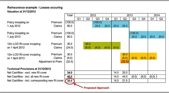
4.3.1. Example 1
Assume a (re)insurer has LOD reinsurance cover incepting on 1 April following a 31 December valuation. The calculation of net technical provisions could:
∙ exclude the reinsurance cover;
∙ include the reinsurance cover in totality (which is unlikely to be realistic or acceptable); and
∙ include the reinsurance cover using correspondence.
The table 1 considers the options:
LoD Example
All claims (whether occurred or not) from the policy incepting on 1 July 2012 must be included within the valuation as at 31 December 2012. Claims from the policy incepting 1 July 2013 will not be included as the contract was not classed as “existing” as at the valuation date.
Though the LOD reinsurance cover commencing 1 April 2013 does not strictly “exist” as at the valuation date, we recommend that the portion relating to cover for the 1 July 2012 policy is taken into account. Assuming an even allocation of reinsurance cost to the periods of cover, the example above shows an adjusted premium of 30−(3×30/4)=7.5, and recoveries of 6.0 for Q2 2013. This then gives a net cash flow out-flow of 20 [claims]+7.5 [adjusted reinsurance premium]−6.0 [reinsurance recoveries]=21.5.
The recommended approach is considered to be more realistic. This approach is also likely to increase technical provisions compared with an approach that excludes the reinsurance contracts that do not strictly “exist”.
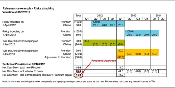
4.3.2. Example 2
Assume a (re)insurer has a 12-month RAD reinsurance cover that will incept on 1 January following a 31 December valuation but which is “legally binding” by the valuation date. The calculation of net technical provisions could:
∙ exclude recoveries in respect of future inwards policies and adjust RI premiums for correspondence;
∙ include the RI recoveries and premiums in full (this is unlikely to be considered realistic); or
∙ include the RI recoveries and adjust RI premiums.
The table 2 considers the options:
RAD Example
As the second RAD cover would only respond to any inwards contract incepting in 2013, of which none are contained in the valuation as at 31 December 2012, the recommended approach is to exclude all recoveries and adjust reinsurance premiums from this contract, which is considered to be more realistic. This approach is potentially open to more debate as it excludes recoveries for a contract that would strictly fall within the definition of an “existing” contract (though the recoveries excluded are driven by a contract that does not “exist”). This approach may appear less obvious than Example 1 but does ensure consistency between approaches. The rationale for the proposed approach in Method 1 is considered strong.
The contract may still be included outside of the technical provisions. In this case, the (re)insurer is committed to purchasing the reinsurance contract and the net cash flow (excluding discounting) is −6 (i.e. 30 of premium out with 24 of expected recoveries). This could be booked as a liability of six, relating to reinsurance creditors.
4.4. Gross to Net Simplifications
The calculation of best estimate recoverables can be performed either directly as the probability-weighted average of future recoverable cash flows or indirectly as the difference between the gross and net best estimates.
Solvency II requirements state that the indirect method should only be used if it is expected to produce a result corresponding to the direct method. However, it is expected that this will be a commonly used approach to the valuation of reinsurance recoverables.
One example of this indirect approach is the use of gross to net techniques. These techniques, based on assumptions about the relationship between gross and net liabilities are currently commonly used, and it is expected that (re)insurers will continue to use these. Such simplifications will be acceptable under the rules of Solvency II, but a number of conditions must be met. The overarching requirement is that reinsurance recoverables calculated in this indirect manner are consistent with Article 81 of the Framework Directive (particularly in the allowance for timing differences and an adjustment for counterparty default risk).
The proxies that may be used for these simplifications can generally be grouped into those based on:
∙ historic accounting figures;
∙ gross and net paid claim data; and
∙ gross and net outstanding claim data.
4.4.1. Considerations when applying gross to net simplifications
Gross to net techniques may be used as long as the particular methodology selected is proportionate to the underlying risks. Any methods used must ensure that:
∙ there is correspondence between gross and net best estimates of a homogeneous risk group;
∙ the net calculation is performed at a level that adequately matches the granularity of relevant reinsurance programmes and allows for the relevant features of this cover;
∙ the allowance for counterparty default is reflected appropriately;
∙ claims provisions and premium provisions are calculated separately;
∙ recoveries on WBNI business may need to be considered separately, similarly recoveries on binary events;
∙ calculation methodologies distinguish at least between LoB for premium provisions;
∙ calculation methodologies distinguish at least between LoB and between AYs not fully developed for claims provisions; and
∙ the simplifications are appropriate throughout the year. If the reinsurance programme or the gross business is not written uniformly over the year an appropriate approximation at year-end may be unsuitable at the mid-year, say.
(Re)insurers must ensure that relevant features of the reinsurance cover are adequately taken into account. There may be expert judgement required if the historical factors are to be adjusted to reflect changes in the reinsurance cover available over time. This needs to be done with great care and any assumptions clearly documented. For multi-year cover or reinsurance contracts spanning multiple homogeneous risk groups, gross to net techniques should be calculated at an appropriate level and apportioned.
4.4.1.1. Possible simplifications
Simplifications that could be considered include:
∙ estimating the future reinsurance cash flows by applying the business plan reinsurance to gross premium ratios to the estimated gross future premium cash flows;
∙ estimating reinsurance recoveries on WBNI claims by reference to business plan loss ratios; and
∙ estimating reinsurance recoveries on binary event loads by reference to past catastrophe events.
All the simplifications above require different implicit assumptions, the reserving actuary/specialist should consider the appropriateness of these assumptions to the business being reserved.
4.4.1.2. Situations where simplifications are likely to be acceptable
∙ Net-to-gross techniques are likely to be acceptable for most standard approaches (e.g. where triangles are used), though these will have to be justified.
∙ The choice of netting down factors is subjective, and are based on knowledge of the book and history and are only used where the Actuarial Function has sufficient knowledge and experience.
∙ Where segmenting by homogeneous risk group, line of business (LoB) and claims and premium provisions is possible.
4.4.1.3. Situations where simplifications may not be acceptable
∙ Exposure analyses: Where direct/explicit reinsurance calculations are often available.
∙ Complex outwards reinsurance programmes: Where simple or implicit methods would often be unsuitable.
∙ When consistency with gross calculation is required: For example, if an average cost per claims method is employed. For a frequency severity model, explicit modelling of reinsurance would be preferable.
∙ Where allowing for cover limits or exhaustion is required as simplification may not implicitly capture the risk appropriately.
4.4.2. Proportionality assessment
Draft Level 2 requires that (re)insurers should carry out a proportionality assessment to determine whether gross to net simplifications are appropriate as a valuation method. This assessment includes the following phases:
∙ assessment of nature, scale and complexity;
∙ assessment of proportionality of valuation method; and
∙ back-testing.
4.4.3. Summary
In practice, it is expected that gross to net techniques will continue to be commonly used, as is currently the case. This can, however, also introduce some additional complications, such as determining expected reinsurance payment patterns, which are discussed in section 4.6.
4.5. Direct Calculation of Net Best Estimates
As an alternative, (re)insurers may use a direct calculation of net best estimates (by using net data) rather than applying gross to net assumptions to gross cash flows and best estimates. This methodology may be used under Solvency II, but would require adjustments to the data used to take into account changes in reinsurance cover over time. This may be complicated process and may prove difficult to meet the requirements of Article 81.
4.6. Reinsurance Cash Flow Patterns
4.6.1. Using the timing of gross payments for reinsurance cash flows
A common approach will be to base the payment patterns for the expected reinsurance recoveries on the payment patterns estimated for the underlying gross claims.
Most commonly, the reinsurance payment pattern is assumed to be the same as the gross claims payment pattern. This may considerably simplify cash flow projections. In order to justify its application, (re)insurers should compare the expected timing of their inwards and reinsurance cash flows for the homogeneous risk groups used for calculating best estimates. This assessment should be based on historical experience, as well as expert judgement and external data, where appropriate. Furthermore, the decision to use this simplification should be adequately documented and explained.
The principle of proportionality should be taken into account when considering whether the timing of cash flows is “sufficiently similar”. As well as consideration of the differences in inwards and reinsurance cash flow patterns, this should also include an assessment of the expected impact on net best estimates. The expected impact is primarily through the effects of discounting, so will vary depending on the level of the EIOPA-provided interest rate term structure at the time of valuation. Recently, interest rates have been very low, thus increasing the likelihood that this simplification may be acceptable. However, the reserving actuary/specialist needs to take care to keep this under review as it may cease to be acceptable should interest rates increase in the future.
The focus of an assessment of similarity must be based on the gross and reinsurance payment timings, rather than the gross and net. However, when considering proportionality and the effect on overall net discounted best estimates, the net cash flow pattern can also be useful.
4.6.2. Illustration of effect
One way of describing differences between inwards and reinsurance cash flows is in terms of the lags and differences in overall term of the payment patterns. The following charts illustrate the effects on a simplified net payment pattern.
The gross payment pattern has been based on a simple lognormal distribution with projected cash flows discounted using a risk-free interest rate term structure. Reinsurance recoveries have been based on the same lognormal distribution, but incorporating a shift in the mean and a stretch to the overall term of payments. Reinsurance recoveries have been assumed to be a constant proportion of gross payments over the lifetime of the liabilities.
The two below charts illustrate the effects on the reinsurance and net payment patterns under different assumptions about:
∙ the shift in the mean for the distribution of reinsurance compared with direct payments (effectively giving a shift in the pattern); and
∙ the overall length of the pattern (effectively stretching or scaling the overall time before all reinsurance recoveries are made). In the examples below, the stretch is made evenly across the pattern.
4.6.2.1. Illustration of effect with limited reinsurance and small lags between gross and reinsurance
First, consider a situation where the mean shift from the gross to the reinsurance payment is small and there is little difference in the overall length of the development pattern. The timing of reinsurance cash flows will be very similar to those of gross cash flows. In this case, the conditions for using the direct pattern for the recoveries would presumably be met. The relative levels of discounting applied to both gross and reinsurance cash flows would be similar.
In addition, if reinsurance recoveries are a small proportion of gross payments (20% in this example), the overall effect on the net discounted best estimates of using the gross payment pattern would not be material. The derived net cash flow pattern would then be very similar to the gross, showing that the relative level of discounting applied within gross best estimates and the overall net best estimates are similar. This lack of a material impact would support the use of the simplification.
The Figure 3 illustrates this effect.
Illustration of Effect with Limited Reinsurance and Small Lags Between Gross and Reinsurance
4.6.2.2. Illustration of effect with more significant reinsurance and longer delays from gross payments
The chart below considers a situation where reinsurance recoveries occur significantly later and take longer to develop than gross payments. In this situation, the timing of reinsurance payments is significantly different and the simplification would not be appropriate. The chart below uses a reinsurance pattern following the same lognormal distribution as the gross, but with a larger shift in the mean and a larger scaling. In addition, if reinsurance recoveries are a large proportion of gross payments (60% in this example), the net best estimate would be significantly affected by applying the gross cash flow pattern to reinsurance payments. Note that because reinsurance is a large proportion of gross, and there is a significant lag between gross payments and recoveries, the net development pattern exceeds 100% of ultimate for many periods. The graph highlights this potential pitfall of using net data to define patterns.
Under the principle of proportionality, the differences between net best estimates with reinsurance payments using the gross cash flow pattern versus a separate reinsurance pattern would mean that the simplification would not be appropriate.
Illustration of Effect with More Significant Reinsurance and Longer Delays from Gross Payments
4.6.3. Worked examples
It is recommended that (re)insurers perform the sort of analysis detailed below to assess whether the assumption that the reinsurance and gross cash flow patterns are “sufficiently similar” and whether the simplification is appropriate. We would expect (re)insurers to consider three key factors:
∙ the extent to which the reinsurance cash flows are shifted from the direct payments;
∙ the extent to which the whole development pattern is stretched; and
∙ the overall effect on the discounted net best estimates.
The final point is most significant and should be considered to over-ride the first two, even if the pattern does not look significantly different (see Example 1b below for illustration of this).
The following examples are intended to illustrate the sensitivity of net best estimates to differences between the gross and reinsurance patterns, under the simplification that reinsurance recoveries follow a gross cash flow pattern.
The examples use simple cash flow patterns that follow lognormal distributions (with gross patterns fitted to real-world data), with the differences between gross and reinsurance patterns defined in terms of a shift from the gross mean duration and a stretched overall payment term (with total payment term actually defined in terms of the time difference between 1% and 99% developed to avoid distortion and make the periods reasonable).
The net best estimate where gross and reinsurance cash flow patterns are identical (i.e. a mean shift of 0 and a pattern length that is not stretched) have been normalised to a value of 100.
4.6.3.1. Example 1a: short-tail LoB with limited reinsurance
The following example considers the overall impact on net best estimates for a short-tail LoB with limited (in this case 20% proportional) reinsurance cover. Table 3 sets out the calculated net best estimates under a number of assumptions about the difference from the gross cash flow pattern and the reinsurance recovery cash flow pattern.
Impact of Differences Between the R/I and Gross Payment Patterns: Short-Tail with Limited R/I
The green cell above represents the net best estimate with reinsurance recoveries following the same development pattern as the direct payments. This has been normalised so that the net discounted best estimate if the reinsurance cash flow pattern is identical to the gross is 100. This base pattern shows a time difference between time when payments are 1% and 99%, developed of 11.5 years.
The blue cell, selected as an example only, represents the value of the net discounted best estimate if the underlying reinsurance recovery pattern has a mean duration that is 2 years longer (mean shift of 2.0), followed by a similar stretch to the pattern (with a difference between the time when the pattern is 1% and 99%, developed now at 14.5 years). The net discounted best estimate is 102.7 or 2.7% more than the best estimate obtained using the gross pattern for recoveries.
The cells highlighted with red text represent those combinations of differences in the reinsurance and gross cash flow patterns that result in a 5% or greater difference from the net best estimate with no difference in patterns. The threshold of 5% has been chosen arbitrarily for purposes of illustration.
As can be seen, even if the reinsurance pattern is significantly different from the gross pattern, the overall impact on the net best estimates is not marked. Therefore it is envisaged that simplified approaches or assumptions could be applied in practice under these conditions.
The concept of applying a variation on the proposed simplification (i.e. rather than use the gross inwards pattern directly the idea would be to use the gross pattern but with a simple lag or stretch) may be a suitable alternative to the pure simplification.
4.6.3.2. Example 1b: short-tail LoB with significant reinsurance
The following example considers the overall impact on net best estimates for a short-tail LoB with significant (in this case 60% proportional) reinsurance cover. Table 4 sets out the calculated net best estimates under a number of assumptions about the difference from the gross cash flow pattern and the reinsurance recovery cash flow pattern.
Impact of Differences Between the R/I and Gross Payment Patterns: Short-Tail with Significant R/I
As can be seen from the pattern of cells that are highlighted above, the differences between gross and reinsurance cash flow patterns are significant, even if the reinsurance pattern is not particularly different from the gross. The simplification would not be appropriate and more risk-sensitive methods should be used.
4.6.3.3. Example 2a: long-tail LoB with limited reinsurance
The following example considers the overall impact on net best estimates for a long-tail LoB with limited (in this case, 20% proportional) reinsurance cover. As in the previous examples, Table 5 sets out the calculated net best estimates under a number of assumptions about the difference from the gross cash flow pattern and the reinsurance recovery cash flow pattern.
Impact of Differences Between the R/I and Gross Payment Patterns: Long-Tail with Limited R/I
As can be seen from the pattern of cells that are highlighted above, the differences between gross and reinsurance cash flow patterns are not significant in most of the table, even if the reinsurance pattern is very different from the gross. This should mean, under the principle of proportionality, that the simplification or similar simplifications would be appropriate in many cases (though perhaps not with combinations of mean shift and difference in length of pattern that are too extreme).
4.6.3.4. Example 2b: long-tail LoB with significant reinsurance
As can be seen from the pattern of cells that are highlighted above, the differences between gross and reinsurance cash flow patterns are significant, even if the reinsurance pattern is not particularly different from the gross. Whether this simplification is appropriate should be considered under the principle of proportionality and in light of overall uncertainty in the reserves. Assuming the overall uncertainty is not particularly high, the simplification would not generally be appropriate.
Impact of Differences Between the R/I and Gross Payment Patterns: Long-Tail with Significant R/I
4.6.4. Conclusion
The examples given above illustrate that the most important consideration is the amount of reinsurance, as would be expected. If reinsurance recoveries are expected to be large, then assuming that reinsurance recoveries follow the gross payment timings is unlikely to be appropriate. This would be the case even if the actual differences between the patterns are relatively small. The reserving actuary/specialist under Solvency II would need to consider these factors carefully in deciding on the approach to take for technical provision valuation regarding reinsurance recoveries. The approach taken should be carefully documented and justified. In summary:
∙ when reinsurance is low, the discounted net reserves are fairly insensitive to the differences between gross and reinsurance cash flow patterns and so the simplified approach would be acceptable; and
∙ when reinsurance is high, the results are far more sensitive and this assumption becomes inappropriate.
There are many circumstances where reinsurance recoveries may not follow a simple pattern and more explicit and potentially subjective estimation will be required, for example, relating to catastrophes or very large claims. In this instance, more of an exposure-type approach will be adopted and payments can be assumed to be more stepped and not follow a pattern. This will tend to be based on expert judgement more than the general pattern approach.
4.7. Allowance for Counterparty Default
Under Solvency II, recoverables from reinsurance and Specialist Purpose Vehicles (SPVs) must be adjusted for expected losses owing to counterparty default. This adjustment should approximate the expected present value of the losses whether due to insolvency, dispute or any other reason. This is no different from current reporting requirements.
The important difference from current approaches for reporting is that the assessment for counterparty default must now be made on a cash flow basis, taking into account the timing of defaults. The determination of the adjustment should take account of default events during the whole run-off period of the recoverables. The adjustment for default must take into account the risk that counterparties survive some years and default at some other point in the whole run-off period of the recoverables. In particular, it is not sufficient to multiply the expected loss owing to immediate default by the probability of default over the current year.
The counterparty default adjustment should be calculated separately at least for each LoB, counterparty and (for non-life) separately for premium provisions and claims provisions. This is likely to require the allocation of reinsurance premiums and claims to class of business. An allowance must also be made for the reinsurance recoveries assumed on additional provisions in respect of future and unincepted premiums.
A separate calculation of default by counterparty may be onerous, especially if the expected loss is small. Where the probability of default and recovery rate of several counterparties coincide, and if calculations at the level of individual counterparty are an undue burden, then the adjustment for these counterparties could be calculated together.
Where the (re)insurer has an internal model, the reserving actuary/specialist will need to ensure that the approach used for counterparty default risk is consistent with that used in the internal model. This may present additional challenges if the approach has been developed independently. On the other hand, it may be an opportunity for the reserving actuary/specialist to adopt a more sophisticated approach, perhaps utilising stochastic modelling, to this element of the reserving calculations.
4.7.1. Simplifications
A full calculation by individual counterparty will be time-consuming and potentially complex.
A suggested simplification, based on proportionality, is to
∙ assess the counterparty risk as a simple deterministic value based on the estimated mean term of cash flows (as opposed to a pure cash flow analysis);
∙ group counterparties together by credit ratings and value the risk of the group (as opposed to individually);
∙ use a deterministic probability of default to apply to the whole exposure (as opposed to varying by time); and
∙ use a static single estimated recovery rate in the case of a failure (as opposed to a random variation).
This approach is similar to current techniques and it is expected that many (re)insurers will elect to use the simplification suggested. This is likely to result in similar groupings to current practice.
In many cases this simplification would be appropriate and is given as:
 $${Adjustment}\,{\rm for}\,{counterparty}\,{default}={\minus}\max \left( {\left( {1{\minus}{RR}} \right){\times}{BE}_{{{\rm Rec}}} {\times}{Dur}_{{{\rm mod}}} {\times}\left( {{{{ PD}} \over {{1\minus{\hyphen}PD}}}} \right)\,,\,0} \right)$$
where RR is the recovery rate of the counterparty; BE Rec the best estimate of recoverables before the expected loss because of default of the counterparty; Dur mod the modified duration of the recoverables; PD the probability of default of the counterparty for the time horizon of one year.
4.7.1.1. Appropriateness of the simplification
The simplification may only be applied if the adjustment can be expected to be small and there are no indications that the simplification formula leads to a significant underestimation.
The formula given above highlights the factors that will drive whether or not the simplification would be appropriate. The examples below further illustrate the effects of varying these factors. These examples are based on the same simple cash flow model, as described for discussion of reinsurance delays, and demonstrate the effects under a situation of short- and long-tail business (and therefore small and large duration) and for reinsurers of a high- and low-credit rating. The calculations use the same patterns as the illustrations in the previous section and, for simplicity, use the scenario where reinsurance cash flows are assumed to coincide with the direct payments.
All calculations have assumed a 50% recovery rate. Note that the amount of reinsurance (which is assumed to be proportional) will not affect the differences in these examples.
4.7.1.2. Example 1: short-tail LoB
Table 7 shows that, as expected, when the underlying probabilities of default are low (e.g. <1%) then the differences between the simplifications and the true value for counterparty default is small. Hence the simplification would be appropriate.
Effect of Simplification on the Allowance for Counterparty Default – Short-Tail
Effect of Simplification on the Allowance for Counterparty Default – Long-Tail
4.7.1.3. Example 2: long-tail LoB
Although the differences are larger for the longer tail classes the conclusion is broadly the same, i.e., that the simplification holds in most instances where the underlying reinsurance security is good.
4.7.1.4. Conclusion
The simplification formula itself defines how the simplified calculation would differ from a full calculation with changing parameters. This is illustrated by the tables above, which highlight that the differences between the simplified and calculated allowance are small for lower probabilities of default. However, it is clear that use of the simplification becomes less appropriate for liabilities of a longer duration where probabilities of default are high.
In addition, another assumption required for this simplification is that there is one probability of default that remains constant over time. With a small duration and low initial probability of default, this assumption may be reasonable. However, over a longer period of time, (re)insurers may expect the probability of default to increase for cash flows further into the future.
The simplification is effectively an extension of the current common approach to counterparty default risk where it takes the form of “factor” multiplied by “expected recoveries” where the factor is based on the credit rating of the reinsurer.
4.8. Allocation of Reinsurance to Class
Net best estimates will need to be produced by LoB. Calculation of reinsurance recoverables at the minimum levels of segmentation may be difficult for reinsurance spanning multiple LoB/currencies.
The recoverables expected from whole account reinsurances will need to be allocated to LoB to be able to calculate net best estimates at the level of segmentation required. Expert judgement will be required and underlying assumptions documented, including validation of assumptions.
Multi-year reinsurance contracts may be in place, but may be covering policies that are not yet a contractual obligation of a (re)insurer. Any (future) premium for reinsurance that covers future contacts as well as existing contracts should have such costs apportioned and only the proportion relating to existing contracts (whether incepted or not) included.
This is consistent with the principle of correspondence that underlies the calculation of reinsurance recoveries.
4.9. Other Relevant Factors
Further factors that must be taken into account in the treatment of reinsurance under Solvency II include the following. These are not covered in detail here, but the potential implications for the calculation should be understood.
4.9.1. Accounting for cash flows related to reinsurance recoveries
The calculation of reinsurance provisions should include at least:
Cash in-flows:
∙ recoverables from reinsurance and SPV contracts in respect of claims payments;
∙ recoverables from reinsurance and SPV contracts in respect of allocated claims expenses; and
∙ revenues from reinsurance commission and profit sharing arrangements (from technical sources relevant to individual reinsurance contracts).
Cash out-flows:
∙ future premiums payable for or in respect of reinsurance and SPV contracts; and
∙ if relevant, out-flows from profit sharing arrangements.
Expenses related to the internal processes for reinsurance and SPVs (such as administration or management) should be allowed for in the expenses forming part of the gross best estimate.
One important consideration is for consistency between expected reinsurance recoveries and future premiums, especially items such as reinstatement premiums.
4.9.2. Accrued reinsurance assets
All estimated future recoverables from reinsurance contracts should be allowed for.
However, any recoveries due on paid gross claims (i.e. those where collection notes have been sent out but not received often referred to as “reinsurance accruals”) are part of the Solvency II balance sheet but do not sit within the assets relating to technical provisions and are outside the scope of this paper. In other words, the principle of correspondence should be followed.
Any deposits made in respect of the reinsurance cash in-flows or out-flows must be shown separately in the balance sheet. In this case, suitable adjustments must be made to the recoverables to avoid any double counting.
4.9.3. Collateral against counterparty default allowance
Instruments used to mitigate the effects of counterparty default risk (e.g. collateral or letters of credit) should be taken into account in the adjustment for counterparty default, but any associated credit risk must also be taken into account. The default risk of the underlying instrument should be included as equivalent to the default risk of the reinsurance.
One solution is to assign the credit rating of the underlying collateral to the reinsurance rather than the credit rating of the reinsurer but only to the extent any collateral exists (i.e. it may not cover all the expected recoveries).
4.9.4. Set off
The cash flow projection used in the calculation of the best estimate shall take account of all potential cash in- and out-flows required to settle the insurance and reinsurance obligations over their lifetime. Therefore, all cash flows incurred in meeting liabilities should be identified and valued but there is no explicit requirement to calculate all cash flows separately. However, the best estimate must be calculated gross, with separate calculation of the amounts recoverable from reinsurance contracts and special purpose vehicles.
A common concept is set off where potential inwards claims are “set off” against outwards recoveries (and vice versa) with only the net effect booked. When moving to a cash flow basis, it may be appropriate to include the full inwards and full outwards expected cash flows. This would depend on materiality but the reserving actuary/specialist will have to consider (if relevant).
4.9.5. Non-traditional triggers
Where recoverables from special purpose vehicles depend upon external indicators (such as a parametric trigger), rather than directly indemnifying for losses, allowance for recoveries related to either claims or premiums provisions should only be taken into account to the extent that they can be verified in a “deliberate, reliable and objective manner”. The basis risk of the contract not being triggered must also be considered. In addition, only payments related to underwriting risk should be accounted for in recoverables. All payments that do not relate to underwriting risk (e.g. those that relate to market risk) should be accounted for elsewhere.
4.10. Overall Reinsurance Summary
Reinsurance provisions need to be calculated separately from gross under Solvency II. There are many practical challenges facing (re)insurers, especially the reserving actuary/specialist in assessing the reinsurance provisions. The main challenges can be summarised as follows:
∙ Current methods and simplifications such as gross to net ratios will still be applicable in many circumstances under Solvency II. However, the reserving actuary/specialist will need to justify carefully why this may be the case. Likewise, the reserving actuary/specialist must also decide when to use more sophisticated or explicit approaches.
∙ When selecting the reinsurance contracts to include in the valuation of technical provisions, the principle of correspondence should apply. This can involve inclusion of reinsurance contracts that are to be purchased and would be included as “future management actions”.
∙ Developing reinsurance cash flows may be more problematical than the corresponding gross calculations due to more restricted data. One potential simplification is to set the reinsurance pattern equal to the gross or to make a simple adjustment based on a “lag” or “stretch” approach. As expected, these simplifications will be more applicable the lower the impact reinsurance has on the net results.
∙ An alternative is to use net patterns and derive the reinsurance as the difference between the gross and net. This approach requires caution, especially when reinsurance lags the gross or is material as the net patterns can be distorted.
∙ Allowance for reinsurance bad debt needs to be included, which is no change to current requirements. However, moving to a cash flow basis may potentially require more detailed calculation given that probabilities of default will increase over time. Current approaches (which tend to be “factor” times “expected recoveries”) or the proposed simplification are expected to be applicable in cases where the underlying reinsurance security is strong and associated probabilities of default are low.
∙ The reserving actuary/specialist will need to ensure all the required elements are included in calculations of the reinsurance provisions (e.g. claims, premiums and expenses). This will extend to ensuring a consistent approach to valuing the expected reinsurance recoveries and potential future reinsurance premiums and especially reinstatement premiums.
∙ Reinsurance recoverables that have been settled and notified sit outside of the technical provisions.
∙ At times, reinsurance recoveries may need to be calculated at a different level to the inwards homogeneous risk groups or even spanning multiple Solvency II lines of business. This may be needed to reflect the reinsurance programme in place, for example whole account quota share or stop loss contracts. In these circumstances, allocation is required and pragmatic approaches with justification are recommended.
∙ As is currently the case, a number of other factors will need to be considered by the reserving actuary/specialist when valuing reinsurance technical provisions, these include:
○ Any collateral underlying reinsurance
○ Any set off between inwards and outwards obligations to the same principles
○ Any commutations
○ Any large claims and other cases where reinsurance is calculated explicitly
5. Expenses
5.1. Introduction
When calculating technical provisions, all future expenses that will be incurred in servicing existing insurance and reinsurance obligations should be taken into account. This includes administrative expenses, investment management expenses, claims management expenses (including claims handling expenses) and acquisition expenses (including commissions).
This is a step change in terms of complexity, as for IFRS/GAAP typically only unallocated loss adjustment expenses (“ULAE”) are explicitly considered as a separate expense item within the technical provisions, with “ALAE” usually included as part of the projected claim ultimate amount.
5.2. Relevant Extracts from the Guidance
5.2.1. Solvency II Directive, Article 78: Other elements to be taken into account in the calculation of technical provisions (extract)
In addition to Article 77, when calculating technical provisions, insurance and reinsurance undertakings shall take account of the following:
(1) all expenses that will be incurred in servicing insurance and reinsurance obligations;
(2) inflation, including expenses and claims inflation;
(3) ....
5.2.2 Solvency II Directive, Paragraph 55 (extract)
… the value of technical provisions should correspond to the amount which another insurance or reinsurance undertaking (the reference undertaking) would be expected to require to take over and fulfil the underlying insurance and reinsurance obligations. The amount of technical provisions should reflect the characteristics of the underlying insurance portfolio. Undertaking-specific information, such as that regarding claims management and expenses, should therefore be used in their calculation only insofar as that information enables insurance and reinsurance undertakings better to reflect the characteristics of the underlying insurance portfolio.
5.2.3. EC Draft L2, Article 17, TP 5
… Unless otherwise stated, assumptions underlying the calculation of technical provisions shall be based on the characteristics of the portfolio of insurance and reinsurance obligations, where possible regardless of the undertaking holding the portfolio. Undertaking-specific information, including information on claims management and expenses, shall be used in the calculation only insofar as that information enables insurance and reinsurance undertakings to better reflect the characteristics of the portfolio or where the calculation of technical provisions in a prudent, reliable and objective manner without using that information is not possible.
5.3. Principles
5.3.1. Expense cash flows
Under Solvency II, the best estimate provisions should reflect all future cash flows arising from expenses that will be incurred servicing existing policies during their lifetime.
This includes (but is not limited to):
∙ administration expenses, including:
○ salaries;
○ property costs (including rent, depreciation, heating, lighting, cleaning);
○ IT costs; and
○ expenses in relation to the management (actuarial, finance, risk, commercial, data) or administration of reinsurance contracts or SPVs.
∙ other administration expenses;
∙ investment management expenses;
∙ claims management expenses (including claims handling expenses);
∙ acquisition expenses (including commissions);
∙ costs associated with arranging and managing outwards reinsurance; and
∙ insurance premium tax.
5.3.2. Calculation of expense cash flows
The guidance (see sections 5.2.2 and 5.2.3) states that the principle is to allow for the expenses that another (re)insurer would be likely to incur if they were taking over the management of the business at the valuation date. We assume that this ignores the costs of any transfer of the business between (re)insurers. Thus, the expense assumptions should be appropriate for the reference undertaking (new (re)insurer) and not necessarily the same as those of the (re)insurer for whom we are calculating the technical provisions. It is still acceptable for the (re)insurer to base the expense assumptions on its own experience provided that this reflects what another insurer might be expected to incur.
In practice, we believe most (re)insurers do and will base their expense assumptions on their own experience. One of the reasons for this is the lack of sufficiently detailed and relevant market data.
The assumptions should only relate to future expenses attributable to business that the (re)insurer is obligated to, in other words, rising from commitments made on or before the valuation date only.
Expense assumptions should include allowance for future cost increases. In particular, assumptions about future inflation should be made, which need to be consistent with the assumptions made elsewhere in the calculation of technical provisions and in the internal model, if there is one. The inflation rate used should be appropriate to the driver of the expense.
Assumptions about cash flows should consider future changes in the environment (such as legal, demographic, medical, technological, social or economic).
5.3.3. Going concern or run-off basis
The expenses which are included in the technical provisions should be assessed on the assumption that the reference undertaking (new (re)insurer) will continue to write new business (i.e. on a “going concern” basis) unless a decision has been made by the existing (re)insurer to cease writing further business, or this is very likely to happen in the near future. If that is the case, a run-off assumption should apply.
5.3.4. Allocation to currency
Future expense cash flows should be expressed in the currency in which they are likely to occur and discounted at the appropriate EIOPA-provided discount rate for that currency.
5.4. Methodology
Ultimately, best estimates are required at a Solvency II LoB level. However, claims reserving is likely to be carried out at more granular homogeneous class of business level. The reserving actuary/specialist therefore has a choice: to allow for expenses at Solvency II LoB level (to the extent that they are not already allowed for in the claims reserves), or to develop expense assumptions at the more granular reserving class of business level. There are arguments in favour of either approach. In practice, it is unlikely initially that expense data will exist at either level because historically it has not been required at this level of detail, e.g., investment expense data may be included in a general administrative charge. Thus, expenses assumptions are likely to be less granular and more approximate than the assumptions used for projecting claims and once made, given they are likely to be fairly broad-brush, can be applied at either level.
The basis of the expense assumptions is likely to be past experience with an allowance for projected future inflation. Differences in the nature of different expense items mean different allocation and projection methods (and therefore different data requirements) are needed. Some expense assumptions should differ as to whether they are to be used for the claims provision or premium provision.
To begin, one must look at historical experience. A (re)insurer’s finance department will usually allocate the (re)insurer’s costs between products or product groups and types of expense (administration, investment, claims (allocated and unallocated) and acquisition, or some variation of this split). However, care needs to be taken to confirm that the Finance allocation is appropriate for reserving purposes. It is possible that the data, and any underlying allocations, were collected for a different purpose, and therefore may not be ideal for reserving. If there are no systems in place to collect data or perform the allocation to the level of granularity required then this is something the (re)insurer should consider implementing to collect these data going forwards.
It may not be appropriate to allow for some historical costs in projecting future costs attributable to obligated business at the valuation date. These may include large one-off expenses such as systems implementation projects and marketing campaigns.
One could argue that, because all of the business one is reserving for is already “on the books” as at the valuation date, then there should be no allowance for marketing costs. This will be different from the internal model where the internal model allows for future new business and therefore must allow for the marketing costs associated with generating that business.
An analysis may already be carried out as part of the new business rating exercise, and may be considered as a basis for premium provision expenses. However, some adjustments may be required to allow for differences in the inflationary impact, cost structure and the exposure period under consideration as we are only concerned with the business that the (re)insurer is obligated to at the valuation date.
Care should be taken when using CY budgeted expenses for technical provisions calculated on an underwriting or year of account basis. For example, the ultimate development of a given year of account may span across more than 2 CYs.
This is a potentially complex issue; expenses allocation has always been a challenging and subjective area, e.g., allocating costs to: different functional areas, new and renewal business, different classes of business. A pragmatic approach is therefore required.
Once done, the reserving actuary/specialist must check that total expense loadings do not exceed overall expected.
Below we discuss possible methods by which different expenses could be allowed for.
5.4.1. Claims expenses
ALAE are typically included in the claims data and therefore implicitly projected as part of the claims projection, i.e., assuming the same payment pattern. Adjustments may be required, however, if the allocated costs are changing as a percentage of reported or paid losses, or if the timing of expenses is expected to be significantly different than that of claims. For the premium provision, they are likely to be allowed for in the loss ratio assumption.
It is unlikely that any data will be available to discern a future payment pattern for ULAE though it seems reasonable to assume these will run-off in line with losses.
It is difficult to come up with a “one size fits all” approach to adapting a (re)insurers ULAE expenses to Solvency II because the definition of what is included in ULAE differs between (re)insurers. The reserving actuary/specialist must take care to allow for this by understanding what is currently included to avoid double counting or omitting expenses.
A common approach to estimate unallocated claims management costs is to look at historic paid unallocated claims management costs and relate them to paid losses over the same period. Typically, adjustments are made to allow for the uneven incidence of expense over the life cycle of the claim, for example, by allowing for different costs on opening and closing. Such an analysis tends to result in a percentage uplift that is applied to total outstanding losses.
A simple approach is to apply a similar uplift factor to the future expected losses, be they true IBNR or premium provision losses. It is reasonable to assume that, usually, the uplift would usually be expected to be higher than for reported claims because all claims due to be notified in the future are unopened by definition and therefore likely to incur higher future expenses on average than known unsettled losses. In addition, any change to the company’s cost structure and the impact of future inflation on both loss and costs would need to be considered if materially different.
5.4.2. Acquisition expenses
Given that technical provisions are calculated on a cash flow bases, it may seem strange that we need to allow for acquisition expenses at all. However, many (re)insurers will have to because we need to allow for business that has been accepted before the valuation date for which cover has not yet commenced and the acquisition costs may not yet have been paid.
Thus, acquisition expenses assumptions may be required for the premium provision calculation.
Usually acquisition cost assumptions are relatively straightforward to derive and the necessary analysis may already have been done to derive a pricing assumption. Commission is likely to be a large part of acquisition expenses and current commission rates should be reflected in the assumption.
5.4.3. Profit commission
Profit commission, whether or not you choose to define it as an acquisition cost, may be far more complicated to calculate than acquisition costs more generally, because it is based on claims experience.
The (re)insurer may need to allow for profit commission in both the premium and claims provision. The appropriate approach will depend upon the terms and the timing of profit commission payments. Some profit commission payments may be known, or estimated with reasonable certainty and the date upon which they are due may be fixed at some point in the future, e.g., a contract anniversary. Others may be quite complicated to estimate accurately owing to a complex relationship with future claims experience. In this case, it may be worth considering possible simplifying methods and/or assumptions on the grounds of proportionality.
5.4.4. Administration expenses and overheads
The best estimate needs to allow for all expenses that will be incurred including future administration costs and overheads.
If budgeted expenses are available, and are best estimate, these may be suitable to be used to derive loadings to cover administration and overheads. One needs to check whether they are appropriate. Questions the reserving actuary/specialist might ask include:
∙ Are they best estimate?
∙ Do they include allow for anticipated efficiency improvements?
∙ Do they include any one-off costs, such as implementation of new systems or processes?
∙ Is the allowance for inflation in costs appropriate?
∙ To what period do the budgeted expenses apply? Do we need to adjust them so that they are suitable for the exposure period we are considering?
Care needs to be taken to ensure that expenses are not double counted or omitted.
If it is not appropriate to use the budgeted administration expenses, the expenses can be projected based on historical figures, for example, as a proportion of earned premium.
Depending on the source of administration expenses, these could be allocated using in-force policy counts, relative staff hours spent on different lines, unearned premiums or volumes of best estimate provisions.
As administration expenses are defined as expenses incurred servicing existing business a proportion of these expenses may be attributed to the run-off of existing policies. In addition, we may wish to remove any non-recurring or “one-off” costs from the expenses.
The (re)insurer may decide that a loading for administrative expenses should apply to the premium provision only. This can be appropriate if one is confident that all of the expenses relating to the ongoing management of incurred claims are included in loadings applied to the claims provision. Whether this happens depends very much on how overheads (general management, finance department, actuarial department, internal audit, etc.) costs are allocated. It is not reasonable to assume that all of these overheads need to be carried by future exposure. To check that the balance is appropriate, one might consider the hypothetical scenario where the liabilities relating to past exposure (covered by the claims provision) and the liabilities relating to future exposure (covered by the premium provision) were to be passed on to two different reference (re)insurers who continue to write new business. Would the loadings for expenses in each of the claims and premium provisions be sufficient to cover the expenses for each reference (re)insurer?
5.4.5. Investment expenses
Investment expenses cannot be allowed for by reducing the discount rate.
Investment expenses could be allocated based on the level of funds under management; they could be split into Solvency II classes using (net) best estimate provisions.
5.4.6. Reinsurance costs
The costs associated with purchasing and managing reinsurance should be allowed for in the gross claims and premium provisions. As the technical provisions are calculated on a cash flow basis, one would generally allow for expenses as and when the cash flows occur. However, as discussed in section on Reinsurance, in applying the principle of correspondence, one may have to adjust expense cash flows associated with reinsurance so that only those relating to reinsurance cover corresponding to the inwards risks that the (re)insurer is obligated to at the valuation date are taken into account.
5.4.7. Allocation to currency
Strictly speaking, the expenses should be estimated in the currency in which they will be incurred and discounted at the appropriate EIOPA-provided discount rate for that currency. In practice, this may be difficult to do accurately: for example, some expenses may be head office and based in the currency there, others such as loss adjustors costs may occur in the currency where the risk is based. On grounds of proportionality, the (re)insurer is likely to adopt a pragmatic approach using simplifying assumptions that do not have a material impact on the overall technical provisions. Some sensitivity testing may be required to demonstrate that the impact of the simplification is not material.
6. ENID (Binary Events)
6.1. Terminology
In this section we are going to discuss the (additional) amount that needs to be included in the best estimate claim liabilities (premium and claims provision) to ensure that the best estimate is a true best estimate of all possible outcomes, as opposed to something less, such as a best estimate of all reasonably foreseeable outcomes.
There is no official terminology for this amount. It has had a number of names, the most popular being:
∙ binary events (reflecting the need to allow for both possible positive as well as negative future outcomes); and
∙ extreme events (because that it what it often boils down to, although this is perhaps an over-simplification).
Recently, we have come across a new term that we feel better represents what the reserving actuary/specialist is trying to achieve. The term is ENID: Events Not In Data and it is this term we use throughout this paper.
6.2. Introduction
The allowance for ENID is a contentious issue with insurance professionals taking a wide range of views on how to allow for them and, indeed, whether they should be allowed for at all.
The issue arises because Solvency II requires the (re)insurer to allow for all possible outcomes in setting its technical provisions and not just the reasonably foreseeable or some other subset. This is a change from the approach generally adopted in reserving for statutory accounting and other purposes. In theory, it means that one needs to allow for possibilities that one may not have experienced before either within the (re)insurer or across the entire insurance industry.
6.3. The Guidance
The concept of ENID developed from the original Solvency II Directive definition of best estimate as the (discounted) probability-weighted average of future cash flows. This has been expanded on subsequently by EIOPA/CEIOPS explanatory text and advice, Groupe Consultatif comments and Lloyd’s guidance. This definition differs from that specified in IFRS/GAAP, and the current basis for Lloyd’s Statements of Actuarial Opinion.
Given the lack of consensus to date in how we should allow for ENID, we have decided that it would be useful to bring together, in one place, the relevant publically available guidance to help readers to form their own view.
We note that neither the Solvency II Directive nor the EC Draft L2 refers directly to an ENID loading being required.
6.3.1. Solvency II Directive: Article 77 (2)
The best estimate shall correspond to the probability-weighted average of future cash-flows, taking account of the time value of money (expected present value of future cash-flows), using the relevant risk-free interest rate term structure.…. The cash-flow projection used in the calculation of the best estimate shall take account of all the cash in- and out-flows required to settle the insurance and reinsurance obligations over the lifetime thereof.
6.3.2. Groupe Consultatif: Valuation Of Best Estimate Under Solvency II For Non-life Insurance Interim Report
With the best estimate being the probability weighted average of future cash-flows, some weight has to be given to losses with low probability but high cost within the best estimate valuation. We call these ‘binary events’. This will be a change as the majority of companies currently consider these types of risk as part of their capital assessment rather than best estimate reserves. Examples of binary events include the occurrence of a new type of latent claims or a change in legislation impacting claims payment retrospectively; or a high inflation environment.
6.3.3. CEIOPS Advice: CEIOPS DOC 21/09 CEIOPS Advice for Level 2 Implementing Measures on Solvency II: Technical Provisions: Elements of Actuarial and Statistical Methodologies to Calculate the Best Estimate
This advice was released in October 2009. It includes further discussion of what is meant by “best estimate” and then addresses ENID specifically. The explanatory text on definition of best estimate includes the following:
The Level 1 text states that the best estimate shall correspond to the probability-weighted average of future cash-flows, taking account of the time value of money, using the relevant risk-free interest rate term structure. This in effect acknowledges that the best estimate calculation shall allow for uncertainty in the future cash flows used for the calculation of the best estimate.
In the context of this advice, allowance for uncertainty refers to the consideration of the variability of the cash flows necessary to ensure that the best estimate represents the mean of the cash flows. Allowance for uncertainty does not suggest that additional margins should be included within the best estimate.
The expected value is the average of the outcomes of all possible scenarios, weighted according to their respective probabilities. Although, in principle, all possible scenarios are considered, it may not be necessary, or even possible, to explicitly incorporate all possible scenarios in the valuation of the liability, nor to develop explicit probability distributions in all cases, depending on the type of risks involved and the materiality of the expected financial effect of the scenarios under consideration.
The advice in the document, after a discussion of methodologies, concludes with specific reference to ENID:
Both deterministic and simulation models are parameterised by the historic data available. Regardless of whether a deterministic or simulation model is used, the resulting mean estimates will therefore be based on development similar to that seen in the history and not contain “all possible future outcomes”.
Regardless of the technique, judgement is required in making additions or adjustments to the estimates to allow for circumstances not included in the history that need to be incorporated into best estimates (for example emergence of latent claims, binary events, etc…). In all the methods judgement is an additional element in satisfying article 76 of the Level 1 text.
The wording appears to distinguish between latent claims and ENID.
6.3.4. LTGA and QIS5
The Technical Specifications for QIS5 (July 2010) and the more recent Technical Specification for the Long Term Guarantee Assessment (October 2012) appear to make less of the ENID issue. The following is an extract from both of the specifications.
TP 2.1 The best estimate should correspond to the probability weighted average of future cash-flows taking account if the time value of money.
TP 2.2 Therefore, the best estimate calculation should allow for the uncertainty in the future cash flows. The calculation should consider the variability of the cash flows in order to ensure that the best estimate represents the mean of the distribution of cash flow values. Allowance for uncertainty does not suggest that additional margins should be included within the best estimate.
TP 2.3 The best estimate is the average of the outcomes of all possible scenarios, weighted according to their respective probabilities. Although, in principle, all possible scenarios should be considered, it may not be necessary, or even possible, to explicitly incorporate all possible scenarios in the valuation of the liability, nor to develop explicit probability distributions in all cases, depending on the type of risks involved and the materiality of the expected financial effect of the scenarios under consideration. Moreover, it is sometimes possible to implicitly allow for all possible scenarios, for example in closed form solutions in life insurance or the chain-ladder technique in non-life insurance.
6.4.5. Lloyd’s guidance (March 2011)
Lloyd’s issued detailed technical Provisions Guidance in 2010, updated March 2011. The guidance was built on the earlier material from CEIOPS and Group Consultatif. The guidance included the following illustration of ENID (binary events):
There is a very large range of possible events that could fall into this category. For illustrative purposes, the following list gives some ideas of events that could (but not necessarily would) fall into the category of binary events. Also, depending on an insurer’s risk profile, some of the events may not even give rise to significant losses at all. It is also worth noting some historic events that might fall into this category, the health hazard type of losses such as asbestos and US pollution of the 1980s are prime examples. Other such as the LMX or PA spirals may also be considered to be in this category. There is also the risk of extreme events not included in pricing assumptions impacting the premium provisions for unexpired exposures. Examples of these could be meteor strike, tsunami hitting Florida and unexpected volcanic eruptions.
Products impacting health
∙ Nanotechnology
∙ Aspartame
∙ Electro magnetic fields
∙ GM crops
∙ Nuclear waste
Social/environmental issues
∙ Global warming linked to current polluters
∙ Director liabilities widened
Legislative/political changes
∙ Step change in court rulings (e.g. Ogden tables)
∙ Political intervention
∙ Rulings that ignore underwriting conditions “for the greater good”
Contact/wording issues
∙ Removal of claims made wordings
∙ Retrospective change in conditions (e.g. surplus lines in Florida)
∙ Specific exclusions removed
∙ Not fully understanding exposures
Events
∙ Meteor strikes
∙ Mega volcanoes
∙ Florida tsunami
This list is illustrative but certainly not exhaustive.
Lloyd’s also provided the following suggested methods for allowing for ENID.
The basic concept when allowing for binary events is to remove the truncation inherent in a parameterisation based only on observed historic data. In practice, such an allowance could typically be done in one of three ways:
1. Adjusting the underlying assumptions within the best estimate to ensure the likely impact of the event is included in the projection.
2. Calculating the best estimate reserve separately under the assumptions that a binary event either does or does not occur. The two projections could be combined with a probability weighting.
3. Adding an explicit amount or load to the best estimate excluding binary events.
Currently, methods similar to the first are the most common way of allowing for events outside of the scope of historic data. That is, some allowance for latent claims is often made by selecting more prudent assumptions to take account of the possibility of losses of a scale not contained in the history. In the first and third methods, events would not necessarily be identified explicitly.
One of the underlying principles of Solvency II is transparency, meaning any load or assumption to adjust for binary events should be explicit. The methods chosen should also be relatively simple to avoid spurious results. In most circumstance this would rule out the first method of “just being more prudent” to allow for uncertainty.
Practical suggestions
In reality there are many possible approaches to allowing for binary events. Three are highlighted below:
1. Use history as a guide
Investigate the historical proportional impact on reserves of latent or extreme events. This could be conducted at a line of business level over the last 30 or 40 years. This would be mainly health hazard type claims such as: asbestos, pollution, tainted blood products, silicone implants, Agent Orange, DES, etc.
The result is an estimate of frequency (e.g. X latent claims in 30 years) and severity, average impact is y% of average reserves over the period.
Advantages of this type of approach are that it would give an explicit load for latent/binary claims and is relatively straight-forward to calculate. Disadvantages are that historic events may not be a good guide to future events and that it may not cover “all possibilities”. It would also not necessarily provide an allowance for large events in unearned provisions.
2. Estimate vulnerability to a range of current threats – “scenario” approach
Build a probability and severity database of current possible binary events. These could be explicitly valued and included within the technical provisions calculations.
Advantages of this type of approach are that it would give an explicit load for latent/binary claims and is relatively straight-forward to calculate once assumptions have been made. However, it would be almost impossible to assign realistic probability/severity assumptions for such losses. It would also, by definition, be impossible to allow for “all possible” outcomes.
3. Uplift reserve to allow for limited range of understanding
Actuarial functions use their expert judgement in setting technical provisions and will aim for mean reserves. The resulting mean is expected to underestimate a true mean as it will only include information which is realistically foreseeable. If an assumption is made about the level at which events are realistically foreseeable (e.g. up to a 1:200 year level) then derived uplifts could be applied to estimate a mean allowing for incomplete information.
Using a combination of data available and judgement for fitting a tail, an assumption can be made about the distribution of reserves. This could also be derived using a bootstrap-type methodology.
An assumption can then be made about the likelihood of events included within the data (the 1 in X year events).
For consistency with capital setting, this level for “realistically foreseeable” events could be assumed to be 1 in 200.
An uplift factor can be derived as the ratio of the “true mean” to the “mean only” including realistically foreseeable events. Reserves are calculated using standard techniques and the uplift factor applied.
To illustrate the example, if it is assumed that the reserves estimated using current techniques (i.e. only allowing for reasonably foreseeable events) will exclude the tail of the distribution beyond the 1:200 point and the loss distribution is of a certain type (e.g. lognormal) then the difference between the estimated mean (using current techniques) and the “true” mean can be explicitly calculated and added as a binary event load.
This approach would be subjective and rely on the assumptions made to fit a distribution, approximate the tail of the “true” distribution and about the level of likelihood of events seen in the data. It would be very sensitive to any of these assumptions. The method may also be very sensitive to assumptions about how quickly any such uplift ratios are expected to run-off for older years of account.
It is proposed that, unless further developments are made, method 3 is encouraged and reserves are explicitly uplifted at a Solvency II line of business level to allow for binary events.
Separate uplifts will apply to claims and premium provisions. In all cases the method and allowances for binary events should be well documented.
6.4. What are ENID (Binary Events)?
The term binary events (precursor of ENID) in the context of Solvency II technical provisions is often taken to mean loss-generating events that are high severity and low probability. Such events are often not represented in historical data used as inputs to reserving methods and may be unforeseeable.
The working party would like to propose an alternative definition, one that gets back to first principles and the original wording of the Solvency II Directive. This definition recognises that different insurance entities will already allow for “non-reasonably foreseeable” events to a greater or lesser extent in their “best estimate”.
Thus, the definition that we propose for ENID (binary events) is “the balancing amount required to bring the best estimate before ENID up to an amount allowing for all possible future outcomes”.
Under this definition, ENID loadings will vary not only by the nature of the risks underwritten, but also by the insurer’s reserving policy.
Another point that is not made enough of in the above guidance is that ENID “loadings” should not necessarily mean an increase in reserves. In considering ENID, one should allow for both positive and negative potential future outcomes, not already allowed for. Potential positive future outcomes could include, for example, lower claims experience owing to the successful implementation of a new claims process, a court award in the insurer’s favour or a change in legislation in the insurer’s favour.
6.5. General Considerations in Estimating a Loading for ENID
6.5.1. The starting point
At the time of writing, most (re)insurers are calculating their Solvency II technical provisions by adjusting the reserves calculated for reporting and management information purposes.
In determining an ENID loading (and, indeed, whether one is required at all), in the first instance, the (re)insurer should determine what exposures and risks are included in the “best estimate”, usually estimated based on current reserving practices. If, for example, the (re)insurer’s process is to book an ABE plus an MA, some of the ENID are likely to be considered in the MA. So, provided the rationale for the MA identifies specific (usually adverse) events, these can be brought into the ENID “bucket” or, if not, one must take care not to double count them.
MAs are unlikely to allow for potential positive outcomes (e.g. changes to the terms and conditions or processes to exclude/reduce certain types of claim) and generally represent a margin above the best estimate based on a cautious view. In addition, there may well be potential future events that have not been allowed for explicitly.
Where MAs do not relate to specific events, they are likely to be removed from the Solvency II calculation as margin.
6.5.2. Identifying ENID
One can attempt to identify ENID, as best one can, by bringing together those parties who understand the (re)insurer’s exposure (what has been written, policy terms and conditions, the sort of things that may give rise to claims, etc.) to brainstorm possible future events that could affect the future cash flows. Such parties would potentially include underwriters, claims managers, reserving and pricing actuaries, and reinsurance managers.
Discussion should cover:
∙ factors that could affect future settlements relating to past claim events, reported and unreported; and
∙ factors and potential future claim events relating to the exposure remaining on business the (re)insurer is obligated to at the valuation date.
Note that the exposure period is limited. (Re)insurers need only consider potential future events covered by business that they are obligated to at the valuation date, so, for example, if an insurer writes only annual policies and only accepts new business/renewals within a month of cover commencing, the insurer need only consider potential future claim events over the next 13 months.
The following could be considered:
∙ catastrophe exposure;
∙ potential large one-off claims;
∙ legislative change;
∙ court awards;
∙ other environment changes;
∙ accumulations, etc.;
∙ changes in policy terms and conditions; and
∙ changes in claims processing
Ideally, (re)insurers will need to form a view as to the probability and potential severity of the events considered. Consistency should also be considered with reverse stress testing, the risk register, pricing models, catastrophe modelling and the internal capital model.
Estimation is likely to be subjective and require significant judgement. Evidence to support decisions and assumptions made for ENID could be produced by way of minutes of discussions held and process documentation.
6.5.3. Is it necessary to identify potential ENID?
It is not necessary to identify potential ENID to calculate an ENID loading and, indeed, one could reasonably argue that, for most insurance it is impossible to identify all potential future outcomes. However, there are several persuasive arguments for carrying out the exercise described above, including:
∙ It could be used as the basis for probability/severity approach to calculate an ENID loading.
∙ A loading calculated using a probability/severity approach could be used as a check on an alternate method of calculation, such as a truncated distribution method.
∙ The exercise of “blue sky thinking” about potential risks to which the (re)insurer is exposed has value in its own right in terms of increasing awareness of the risks underlying the business. Those who participate get the opportunity to discuss risk with those of other disciplines and gain a different perspective. They have the opportunity to challenge ingrained perceptions about the likelihood of certain risks and to challenge “closed thinking”. It is likely to produce useful insight into risk and senior management’s attitude to risk and complement other exercises such as reverse stress testing.
∙ Given the insight that can come out of such an exercise, it is likely to be viewed favourably by regulators.
6.6. Methodology
Methods currently used to calculate ENID loadings include:
∙ truncated statistical distributions (as described in the Lloyd’s guidance);
∙ frequency/severity of representative scenarios;
∙ percentage load based on benchmarks and expert judgement;
∙ adjusting reserve parameters;
∙ return period approach; and
∙ no load – existing methods and assumptions already allow for ENID.
Some combinations of these approaches may be used, such as using a frequency/severity method as a check on a truncated distribution approach.
At the time of writing, there is no consensus on methodology.
The truncated distribution approach is based on the assumption that when fitting a statistical distribution around historic claims data, the claims data excludes at least some low probability and high severity events and hence the distribution is truncated. Judgement is used to select the proportion of claims “missing”, e.g., 0.5%. The distribution is adjusted to add to the tail (0.5% in this example) and a new mean is estimated from the new distribution which represents a “true” distribution of claims. The ENID uplift factor applied to the claims is then the ratio of the new mean to the old mean. These uplift factors are likely to vary for claims and premium provisions and consideration should be given to if these factors are applied to either reserves or ultimate claims.
Lloyd’s have adopted this approach to estimating ENID for the aggregate technical provisions calculation although individual managing agents may have adopted different methods.
There are limitations to this approach. For example, sufficient and reliable data is needed or the fitted distribution will lack credibility. Judgement is required to determine what proportion of claims is missing from the historical data and there is usually very little evidence upon which to base this assumption.
However, if one can use this approach, there may be some useful things that come out of it:
∙ It may act as a check on one’s reserve variability exercise: if the result looks ridiculous, then the reserve variability work may be dubious.
∙ There can be real learning in discussing and challenging the distribution fitted, the selection of the cut-off (proportion of claims missing) and the results, in particular, relativities between classes of business.
Consideration should be given to whether loadings that come out the truncated distribution approach should be instead of, or in addition to, ENID loadings for “known” events not in the best estimate.
6.7. Benchmarking
6.7.1. Can we benchmark our ENID loading?
It would be comforting to actuaries and management alike if we could benchmark our ENID loadings. Unfortunately, there are persuasive arguments why, in practice, one is unlikely to be able to, and if one can, care will need to be taken to ensure the comparison is not misleading.
Reasons for exercising care in benchmarking ENID loadings:
∙ Every (re)insurer’s reserving policy will differ. In the same way that (re)insurers may choose different reserves for the same claim, (re)insurers will allow for different things in their IFRS/GAAP “best estimate”.
For example, two (re)insurers may choose to use what they call their ABE as the basis for calculating their Solvency II technical provisions. Blinkered Actuary Re’s ABE may be based purely on historical data. It may ignore the new approach to tackling claims that is expected to reduce future claim settlements by 5% and a legal case that may materially affect the settlement of outstanding claims. This is not a problem because management make an adjustment to the ABE, called the “Management Adjustment” that covers the things that the actuary has not allowed for, plus a “bit of margin for uncertainty”. If Blinkered Actuary Re chooses to use the ABE as their best estimate for Solvency II, their ENID loading will need to allow for the new approach to tackling claims and the legal case (but not for the uncertainty loading).
In contrast, Super Actuary Re, in exactly the same situation, may have an ABE that factors in the legal case, but probably not the new approach to claims. (We are actuaries, after all, and we do like our prudence.) Super Actuary Re’s ENID loading should therefore be different to that of Blinkered Actuary Re.
∙ Every (re)insurer’s business is different, with different exposures, terms and conditions, etc. and hence different exposures to low-probability high severity events.
For example, if a travel insurer covers volcanic ash, they will need to allow for it in their ENID (or best estimate). A travel insurer who does not cover volcanic ash-related claims would not need to.
6.7.2. Available benchmarks
We are not aware of any reliable benchmarks for ENID loadings currently available. Lloyd’s have said that the figures they suggested in the Lloyd’s Technical Provision Guidelines should not be used as benchmarks.
7. Segmentation
7.1. Introduction
As a minimum, (re)insurers must segment their obligations into prescribed Solvency II LoB when reporting technical provisions. In addition, the (re)insurer may need to segment their business by currency in order to apply the correct EIOPA-provided discount rates and/or by geographical location to benefit from geographical diversification in the calculation of the SCR.
There are relatively few Solvency II LoB when one considers the usually far larger number of classes we consider when reserving general insurance business for other purposes, so one might expect that this would not be a particularly onerous requirement. However, the Solvency II LoB do not mirror the way the business is managed, either in relation to technical provisions or capital modelling for many (re)insurers. For example, in the London Market it is quite feasible for a reinsurer not to separate proportional reinsurance from other reinsurance; and UK motor insurers often split experience between bodily injury and property damage claims but not by liability and other as is required for Solvency II. In addition, the need to segment by currency (and possibly by geography, too) means segmentation is an important consideration for many (re)insurers.
It is expected that segmentation into homogeneous risk groups for the underlying reserving calculations will remain largely unchanged. There are a few notable exceptions: UK Motor insurers may choose to split their claims data differently because UK motor covers more than one Solvency LOB; reinsurers may need to split direct and reinsurance business that formerly was reserved together and to split proportional and non-proportional risks; as well as the need to consider currency breakdowns where these may not have been done before.
Data may not currently be collected at the level required for mapping risks to a single Solvency II LoB, which would require apportionments for some classes of business until the required data can be obtained.
It will be the Actuarial Function’s responsibility to decide on applying proportionality with regard to segmentation. Additional data will almost certainly be required to allocate the homogeneous risk groups to currency.
7.2. Guidance
This section is based on the European Commission Draft Implementing measures Solvency II, 31 October 2011 (“EC Draft L2”), paragraphs 3.35–3.52 of CEIOPS final advice for Level 2 Implementing Measures: Technical Provisions, CEIOPS-DOC-22/09 and the guidance issued by Lloyd’s on Solvency II Technical Provisions and Allocation Methodologies. For further information the reader should refer to the detailed advice and guidance.
7.3. General Principles
The fundamental split that should drive the calculation of best estimates within technical provisions is a split into homogeneous risk groups. This will ensure results of any such assessments will be as reliable and credible as is possible. We expect that (re)insurers will use apportionment to get the results based on internal homogeneous classes of business (used to manage the business) to Solvency II LoB.
The principle of substance over form should be followed in segmenting contracts between LoB. In other words, the segmentation should reflect the nature of the risks underlying the contract (substance), rather than the legal form of the contract (form).
This means the approach of performing calculations at a homogeneous risk group level and then allocating appropriately (and with justification) would be acceptable or even expected. (Re)insurers should then use a reasonable basis to allocate business to the Solvency II minimum LoB.
Additional data sources or assumptions may be needed to allocate and report to the required levels. This may include separating direct and proportional business, often modelled together, or separating out facultative non-proportional reinsurance, sometimes modelled with direct business.
7.4. Solvency II Minimum LoB
7.4.1. Non-life
The minimum LoB into which non-life technical provisions must be split are set out below. Annex I of the EC Draft L2 gives fuller description of what is to be included in each LoB.
1. medical expenses insurance;
2. income protection insurance;
3. workers’ compensation insurance;
4. motor vehicle liability insurance;
5. other motor insurance;
6. marine, aviation and transport insurance;
7. fire and other damage to property insurance;
8. general liability insurance;
9. credit and suretyship insurance;
10. legal expenses insurance;
11. assistance; and
12. miscellaneous financial loss.
13–24. proportional non-life reinsurance (relating to insurance obligations included in LoB 1–12);
25. non-proportional health reinsurance (relating to insurance obligations included in LoB 1–3);
26. non-proportional casualty reinsurance (relating to insurance obligations included in LoB 4 and 8);
27. non-proportional marine, aviation and transport reinsurance (relating to insurance obligations included in LoB 6); and
28. non-proportional property reinsurance (relating to insurance obligations included in LoB 5, 7 and 9–12).
7.4.2. Life
The only life LoB likely to be of interest to general insurers are:
33. annuities stemming from non-life insurance contracts and relating to health insurance obligations;
34. annuities stemming from non-life insurance contracts and relating to insurance obligations other than health insurance obligations.
7.5. PPOs and Annuities Relating to Non-Life and Health Policies
If non-life or health insurance policies give rise to the payment of annuities whose valuation requires the use of appropriate life actuarial techniques, the provisions for claims outstanding should be carried out separately for annuities and other claims. For premium provisions, a separate calculation of annuity obligations should be performed if a substantial amount of incurred claims will give rise to the payment of annuities.
Thus, PPOs will need to be reported in LoB 34:
annuities stemming from non-life insurance contracts and relating to insurance obligations other than health insurance obligations.
7.6. Contracts Covering Multiple LoB and “Unbundling”
Contracts covering risks from non-life and life business should be unbundled into their life and non-life parts. Contracts covering risks under different Solvency II LoB should be unbundled or allocated into the appropriate LoB.
Subject to the principle of proportionality, unbundling may not be required in cases where there is one major risk driver. In this case, the contract may be allocated according to the major risk driver. The principle of substance over form may be applied in allocating each of the unbundled components to different LoB.
Unbundling life and non-life parts of some policies may be challenging. This may affect business such as Accident & Health or Travel insurance, where there may also be an amount of life cover. There may also be problems when unbundling non-life contracts where a policy has constituent parts falling within different Solvency II lines. For example, motor policies cover both property and liability risks and some (re)insurers have not reserved separately for each. Where more than one of these parts is material, the proportionality principle means that the unbundling requirement cannot be ignored.
7.7. Currency Groups
The best estimate should be calculated separately for obligations in different currencies on a basis that reflects the underlying liabilities. In many cases, this would be settlement currency but this may not always be the case. The reserving actuary/specialist needs to be clear as to how they have interpreted this requirement and have regard for correspondence between the settlement currency and the underlying liabilities.
For example, if a (re)insurer settles all claims in one currency but the underlying assets supporting the liabilities were held in the original currency (and converted to the settlement currency only on settlement) then the original currency would be more suitable for the liabilities. In this situation, the currency risk in converting the assets offsets the currency risk for the liabilities.
In the working party’s opinion, the key principle is to calculate the best estimate based on homogeneous risk groups. As a consequence of this and the potential lack of credible data at currency level, allocation to currency may be appropriate and is likely to be widely used.
The reserving actuary/specialist should consider whether exchange rates used to convert to settlement currencies are consistent with financial market data on future rates, as per the requirements for validation and selection of assumptions.
The reserving actuary/specialist also needs to consider where premiums, claims and expenses, from otherwise homogeneous group of risks, are in different currencies. In this situation, it may be necessary to make appropriate simplifications taking into account proportionality.
The reserving actuary/specialist must also take care to ensure that any changes to the process to better understand the impact of future currency movements that may affect the level of the reserves, do not lead to data changes that may impact their reserving analyses. That is, actuaries should continue to ensure that data used for projecting (e.g. loss triangles) are prepared on a consistent basis to avoid historical exchange rate movements distorting projections.
Finally, the reserving actuary/specialist must also ensure there is clear communication with the finance team around the treatment of currencies within the technical provisions.
7.8. Geographical Location
Calculation of the non-life SCR for premium and reserve risk can take into account the diversification owing to geographical location of risks. Under the standard formula tested in QIS5, premiums and net best estimates were required to be allocated into one of 18 geographic zones to be able to allow for the impact of this diversification.
Therefore, (re)insurers using the standard formula and who would like to reflect geographical diversification will need to split the results of calculations by homogeneous risk group into geographic zones.
7.9. First Steps
Technical provisions must be calculated using at least the level of segmentation detailed in section 7.4, and for obligations of different currency where material. Homogeneous risk groups are likely to be defined at a lower level of granularity, but may still span Solvency II LoBs. These requirements may mean that class of business groupings used by (re)insurers may need to be adjusted, as well as historic data used as part of the reserving process.
One approach is for the (re)insurer to start with their current classes of business and currency splits. The high-level considerations include:
∙ Do these classes allow for the business to be directly segmented into Solvency II LoB?
∙ Do these splits involve bundled contracts? How significant are the different types of risk covered relative to each other?
∙ What is the most appropriate basis to split into currencies for discounting?
∙ Does the current split leave homogeneous risk groups? Would it result in credible data for reserving?
∙ Do these splits result in all significant currencies (for Solvency II purposes) being calculated separately?
∙ Are there any additional data requirements to meet the Solvency II splits?
∙ Are the proposed splits consistent with the internal model?
7.10. Allocation to Solvency II Level of Granularity
As noted, it is expected that the base projections are often not at the level of granularity required for the required segmentation. In these circumstances, (re)insurers should apply an appropriate allocation methodology to apportion such figures down to the appropriate level of granularity.
7.10.1. Allocation: high-level principles
Homogeneous risk groups should be considered the most important segmentation level for modelling technical provisions and it is this level that should be considered first. In the event that a homogeneous risk group contains risks falling to more than one of the minimum Solvency II LoB, (re)insurers should use reasonable methods to allocate the results of the calculation to these LoB.
There is no mandated allocation methodology and it is the responsibility of each (re)insurer to ensure that the methodology used is appropriate. There are, however, some high-level principles that the reserving actuary/specialist could consider when determining the methodologies to use:
∙ Ensure that there is consistency between projection and allocation methods. For example, where IBNR is projected based on premium then allocations should be based on premiums.
∙ Ensure consistency between gross and net allocations, where appropriate. Outwards reinsurance covers should be allocated in proportion to the gross losses they cover, if practical.
∙ Allocate very large claims, such as catastrophes, individually, especially where any exposure analyses underlie the projections.
In addition, (re)insurers should note that:
∙ proportional allocations (e.g. allocating IBNR between classes based on incurred claims) are reasonable in many situations, although these will need to be validated;
∙ expenses can be split in proportion to claims reserves but not necessarily by currency (if expected to be incurred in a different currency);
∙ allocations are estimates and, as such, there should be reasonable materiality thresholds set;
∙ they must be able to support, justify and document the methodologies used for allocation; and
∙ considerations of proportionality and spurious accuracy are key – where there is a risk of spurious accuracy, a simple (but reasonable) approach is recommended.
Note that the approaches set out in this paper are suggestions only and each (re)insurer should use the allocation methods considered most reasonable for them.
7.10.2. Allocation methodologies
Premium, paid and outstanding claims data should be available by reserving class for use in allocation methodologies. The following section sets out some possible allocation methodologies based on different items. Note that the methodologies will not be appropriate for use in all situations and specific circumstances should be considered before selecting a method.
7.10.2.1. Outstanding claims (case estimates)
IBNR and IBNER will be calculated by (re)insurers using their homogeneous risk groups (often a firm’s own classes of business). Data on outstanding claims may then be used to proportionally allocate the IBNR and IBNER to each of the underlying classes and currencies making up the homogeneous risk group.
Methodologies based on this data may also be appropriate for allocation of some of the expense items, such as future ULAE (and other non-ULAE expenses, depending on their drivers).
Care must be taken when applying this method, especially on immature cohorts where many claims may not have been notified, and also on older cohorts where the number of open claims is small and the impact of individual claims can be significant.
7.10.2.2. Incurred (or paid) claims
Similarly to the above, data on incurred claims may also be used to proportionally allocate IBNR and IBNER between underlying classes and currencies. Calculations based on this information may also be used to allocate elements of the premium provision.
Incurred claims projections are a common base to calculate IBNR/IBNER (i.e. incurred chain-ladder) and may help consistency if used. If paid claims underlie projections rather than incurred then paid claims can be used to allocate reserves from which notified outstanding claims can be deducted to obtain IBNR/IBNER.
7.10.2.3. Premium
Use of premium data may be the most appropriate measure for allocation of some homogeneous risk group best estimates where there is little other data (such as reported outstanding or incurred claims in recent years of account) to base a split on. This will ensure consistency where common projection methods such as Bornhuetter–Ferguson are employed. This is likely to be particularly relevant for elements of the premiums provision where claim events are yet to occur.
Allocation of future premiums may also require use of premium data for the most appropriate split. Note, however, that (re)insurers should consider what is driving the expected future premiums, as a claims measure may be more appropriate for some types of future premiums.
7.10.2.4. Policy-by-policy analysis
(Re)insurers may calculate some of the required best estimate figures directly on a policy-by-policy or exposure basis, for example, for large claims or events. If so, these amounts can be removed from the homogeneous risk group, the remainder allocated using another of the methods, and then the directly calculated best estimates added to the class required.
This is expected for very large claims such as catastrophes that could otherwise distort results materially.
7.10.2.5. Combination of approaches
In line with the high-level principles set out above, the most appropriate methodologies should be used. These would be expected to differ by year of account and class of business and will include a combination of approaches.
The Actuarial Function is expected to either own or have significant input into the decision over what methods to use, and for which years of account; the person responsible for the approaches chosen should be clearly identified and be able to provide justification and evidence.
7.10.3. Allocation to geographical location
Various data sources may be available to perform this split, including specific location data, data on insured’s head office or an allocation based on historic location information. The allocation of outwards reinsurance cover would, in general, be consistent with that of the underlying inwards gross business allocation.
We expect that, once the standard formula is finalised, (re)insurers will need to be able to confirm that the estimated geographical splits are reasonable, especially for worldwide covers where allocations will be needed.
7.10.4. Allocation to currency
(Re)insurers may need to allocate best estimate technical provision elements between currencies where these are not calculated at currency level.
(Re)insurers will probably report in their major settlement currencies but only if there is supporting evidence that this split of settlement currencies does capture all the material underlying currencies. For example, if Australian dollars represents an immaterial currency and is settled in sterling, then this may be reported within the sterling bucket. The key consideration is materiality.
The reserving actuary/specialist needs to be careful where in aggregate, the total of the (individually) non-material currencies become material. In this case, the largest one or two (or three) of the (individually) non-material currencies in those buckets should be identified and reported separately or (re)insurers may choose to analyse all the non-material currencies separately from business that is reported in original currency (e.g. sterling business and non-sterling business converted to sterling could be reported separately).
Splitting the provisions by currency can occur at different stages of the process. Clearly, of there is enough credible data, then it makes sense to split the raw data down to currency before reserving takes place. Where there is no credible data, then allocation may take place before discounting; then the payment pattern derived from the combined data may be used for each currency group together with the correct EIOPA yield curve for discounting. Finally, there is the option of using a blended discount rate to estimate the discounted reserves and then doing the allocation. In using this approach, the reserving actuary/specialist will need to demonstrate that the simplification is appropriate: in particular, that the risk of materially misstating the provision by using the blended discount rate is low. This is most likely in an environment where
∙ the yield curves in the different currencies are very similar;
∙ yields are very low; and/or
∙ the liabilities are very short.
If the impact of discounting does not vary materially between classes to which a homogeneous risk group is being allocated, then, on the grounds on proportionality, a simplified allocation by currency is likely to be acceptable. If there are differences, then adjustments to the allocation methodology may need to be taken to allow for this. This may occur if there emerges a material difference over time between the risk-free yields in different currencies.
7.10.5. Allocation of other elements
There are other elements of the technical provisions that may be more challenging, or require additional assumptions in order to allocate to the required levels. Some of these are discussed below.
7.10.5.1. Expenses
There may be several possible approaches for allocating expenses in a reasonable way. These should consider the drivers of the expense item and also proportionality. For example, premium measures may be the most appropriate way to split the provision for future acquisition expenses between class. The claims elements of claims and premium provisions (i.e. not including the negative impact of future premiums) may be a more appropriate measure to split the claims administration expenses.
It is important to consider the currency features of the expenses that are being split. For example, it may not be appropriate to split out expenses into all currencies if they are actually to be incurred in sterling.
In practice, we do not expect to see very detailed expense allocation. For many classes of business the expenses will be far less material than the claims liabilities and the use of approximate approaches to allocating claims liabilities would make a detailed expense allocation incongruous.
7.10.5.2. Future premiums
If there are expected to be future premiums the reserving actuary/specialist should consider the extent to which these are expected in a particular segment. It may be acceptable to assume that future premiums are likely to be split in proportion with the premiums received to date, but if the balance of the business written recently has changed from the recent past, this assumption may not be acceptable.
7.10.5.3. Reinsurance
The reinsurance share of the technical provisions must also be split by class and currency. In many cases, the approach taken should follow the approach taken for the allocation of the gross best estimates. However, there may be cases where this is not straightforward and more detailed analysis can be carried out to work out more explicitly which class reinsurance recoveries should be allocated to.
A key consideration is consistency between the allocations of gross amounts and reinsurers’ shares to ensure outwards recoveries correspond to the inwards claims. For example, if all the IBNR for a particular class of business is allocated to one class or currency then, in most cases, all the outwards reinsurance IBNR would also be expected to be allocated to the same class/currency.
(Re)insurers will need to consider how to allocate reinstatement premiums across the classes within a homogeneous risk group. A reasonable approach would be to assume that these reinstatement premiums are allocated in the same way as the claims that they are linked to. However, where such reinstatement premiums are considered immaterial, it may be reasonable under a principle of proportionality (and more simple) to allocate these based on the underlying premiums.
Where reinsurance recoveries are defined in a currency that does not match that of the underlying gross claims these should be reported as such. If these are immaterial, the allocation methodology could be allocated in line with the underlying gross claims.
Where reinsurance covers multiple LoB, the reserving actuary/specialist must consider the most appropriate way in which the best estimates of reinsurer share should be allocated to class and currency. This should be based on the expected contribution of the underlying gross business to the expected recoveries. It is recognised that this element can be problematic (as it may depend on timings of losses, etc.), but the key principle remains reasonableness with justification. For example, in most cases, whole account stop loss reinsurance IBNR may be allocated in proportion to the gross inwards IBNRs. That is, it may be reasonable to allocate expected recoveries from whole account covers in proportion to the (already) allocated inwards reserves. However, firms should not expect whole account (or multiline) covers to be allocated to single class/currency splits where the underlying business covered is clearly not.
7.10.5.4. Risk margin
Solvency II requires the risk margin to be calculated at a whole account level. This must then be allocated to the Solvency II LoB, adequately reflecting the contribution of each of LoB to the overall SCR as used in calculation of the risk margin. This allocation may use output from an internal model, if available, or a broad simplification may be appropriate. This is discussed further in section 8.3.
7.10.6. Materiality and complexity of approach
In allocating liabilities to the necessary level of granularity, materiality ought to be a key consideration throughout. Apart from exposure analyses where explicit calculations will exist, in many cases the use of complex allocation techniques may add spurious accuracy.
7.10.7. Simple worked example for allocation
For an example of how to apply allocation, we refer the reader to the simple worked example in the Lloyd’s publication, Solvency II, Technical Provisions Data, Suggestions for Allocation Methodologies.
8. Risk Margin
8.1. General Requirements
The Solvency II Directive: Article 77(3): calculation of technical provisions states that:
The risk margin shall be such as to ensure that the value of the technical provisions is equivalent to the amount insurance and reinsurance undertakings would be expected to require in order to take over and meet the insurance and reinsurance obligations.
Technical provisions for most non-life business will be calculated as the sum of an explicit best estimate and an explicit risk margin. Risk margins should be calculated using a “cost of capital” approach.
The cost of capital approach requires the risk margin to be calculated by determining the cost of providing an amount of eligible own funds equal to the SCR necessary to support the obligations over their lifetime.Footnote 1 This approach is intended to reflect the costs incurred by a notional (re)insurer in raising capital to accept a transfer of liabilities. The calculation is based on the assumption that the “reference” (re)insurer capitalises itself at the time of transfer, t=0, to the required level of eligible own funds:
 $${\rm EOF}_{{{\rm RU}}} {\rm (0)}\,{\rm =}\,{\rm SCR}_{{{\rm RU}}} {\rm (0)}$$
where EOFRU(0) is the amount of eligible own funds raised by the reference (re)insurer at the time of transfer, t=0 and SCRRU(0) the SCR at time t=0 as calculated for the reference (re)insurer.
The cost of providing this amount of eligible own funds is equal to this, multiplied by the assumed annual cost of capital for each future year. The underlying approach is to calculate the insurer’s technical provisions and SCR for each year in the future until the business is fully run-off.
The overall risk margin according to the cost of capital methodology (“CoCM”) should be calculated as follows:
 $${\rm CoCM}={\rm CoC}\,{\times}\mathop{\sum}\limits_{t\geq 0} {{{{\rm SCR}_{{{\rm RU}}} \left( t \right)} \over {\left( {1{\plus}r_{{t{\plus}1}} } \right)^{{t{\plus}1}} }}} $$
where SCRRU(t) is the SCR for year t, as calculated for the reference (re)insurer notionally receiving the transferred liabilities (NB: SCR relates to existing business only); r t the risk-free rate for maturity t; and CoC the cost of capital rate (currently prescribed at 6%).
The SCR should be calculated using either the Standard Formula or an approved Internal Model (whichever is relevant to the firm) and allows for diversification across LoB.
8.2. Risks to Take Into Account Within the Risk Margin
Only the business existing at the valuation date (t=0) is taken into account in the SCR used for calculation of the risk margin. It will include all “current obligations” that are taken into account in technical provision best estimates (including any policies not yet incepted by the valuation date). Specifically, underwriting risk in respect of non-obligated future business (not included within the technical provision best estimate) is not taken into account.
The SCR used for calculation of the risk margin should allow for:
1. insurance risk (both reserve and premium risk) with respect to the obligated business, whether incepted or not. This includes any future premiums and associated exposures;
2. counterparty default risk with respect to the ceded reinsurance and special purpose vehicles;
3. operational risk; and
4. unavoidable market risk.
This is therefore a subset of the actual SCR, ignoring new business and some portion of market risk.
“Unavoidable market risk” must be included. Though assets are assumed to be de-risked under the notional transfer, there would still be some market risk following an assumed inability to perfectly match the cash flows of long-term liabilities. It is not necessary to fully replicate cash flows to eliminate the market risk SCR. Replication of best estimate cash flows is sufficient to reduce market risk SCR to an immaterial level for the purposes of the risk margin calculation. For non-life liabilities and short-term life insurance obligations, the market risk SCR for the risk margin calculation can usually be reduced to zero and hence is all “avoidable”.
Internal models (partial or full) should be used to calculate the relevant elements of the SCR if the firm is using an approved internal model for regulatory capital.
8.3. Calculation of the Risk Margin
The SCR for each future year until business is run-off must be projected. Each of the future SCRs (strictly, subsets of the SCRs) will be multiplied by the cost of capital rate to get the cost of holding these future SCRs.
Each amount will be discounted to the valuation date (t=0) using a risk-free yield curve provided by EIOPA. The sum of the discounted values is the risk margin.
(Re)insurers are still required to calculate risk margins at least at a Solvency II minimum LoB level, based on the segmentation laid down by the implementing measures. The approach suggested is as follows:
1. calculate the risk margin for the whole business of the (re)insurer; and
2. allocate this total risk margin between LoB;
The allocation to LoB should reflect the contribution of each LoB to the overall SCR during the lifetime of the business. A first step in analysing such a contribution can involve calculating the SCR for each LoB in isolation. Where the relative SCRs do not vary significantly over time, there is the following simplification available:
 $${\rm CoCM}_{{{\rm LOB}}} {\rm =}\left( {{{{\rm SCR}_{{{\rm RU,LOB}}} {\rm (0)}} \over {\mathop{\sum}\limits_{{\rm LOB}} {{\rm SCR}_{{{\rm RU,LOB}}} {\rm (0)}} }}} \right){\times}{\rm CoCM}$$
where CoCMLOB is the cost of capital risk margin allocated to line of business, LOB; SCRRU,LOB(0) the SCR of the reference (re)insurer for line of business, LOB, at time t=0; and CoCM the cost of capital risk margin for the whole business.
The cost of capital risk margin is defined net of reinsurance only. Some forms of whole account reinsurance will therefore have to be allocated in a pragmatic and justifiable way to the LoB for calculation of risk margins (as with the calculation of the best estimate). If an internal model is used, the risk margins may be calculated on gross and reinsurance separately, if necessary.
8.4. Cost of Capital Rate
The cost of capital used is an additional amount, above the relevant risk-free rate, that a (re)insurer would incur holding an amount of eligible own funds equal to the SCR necessary to support the run-off of its obligations. In the general methodology set out above, this rate is applied to the subset SCR in each future period. The risk margin should ensure the technical provisions can be transferred even in a stressed scenario. The cost of capital rate should therefore be a long-term rate, reflecting both periods of stability and stress, and should not be adjusted to follow market cycles.
The rate will be the same for all (re)insurers and will be calculated periodically by EIOPA according to a standard methodology. Based on current information, the cost of capital rate is 6% pa.
8.5. Links to IFRS
The development of the next phase of IFRS involves similar concepts to the risk margin under Solvency II. Under the latest proposals, no one method is stipulated for calculating the risk adjustment (although a cost of capital approach is expected to be acceptable). It is likely that this situation will continue and specifically that both Solvency II and IFRS will require a similar but potentially different calculation of the risk adjustment/margin.
8.6. Simplifications
In general, the risk margin calculations and, accordingly, the underlying projection of future SCRs should be as accurate as possible. If a firm is able to carry out a full projection of all future SCRs, for any or all LoB, then it should do so (allowing for proportionality).
However, precise calculation of risk margins is likely to be difficult for many (re)insurers. Simplified methods for the risk margin are expected to be widely used in practice. To allow for this, the following hierarchy of simplifications regarding the methods to be used for projecting SCRs for each LoB should be used. Ranging from the most complex to the simplest, these are:
1. make a full calculation of all future SCRs without using simplifications;
2. approximate the individual risks or sub-risks within some or all modules and sub-modules to be used for the calculation of future SCRs;
3. approximate the whole SCR for each future year, e.g., by using a proportional approach;
4. estimate all future SCRs at once, e.g., by using an approximation based on the duration approach; and
5. approximate the risk margin directly as a percentage of the best estimate;
Before applying a simplified method to calculate the risk margin, the (re)insurer must ensure that the method is proportionate to the underlying risks and compatible with the Solvency II valuation principles. The level of complexity used to calculate the risk margin is not required to go beyond that necessary to capture the risk profile of the business. The (re)insurer must assess whether or not application of such simplifications is appropriate for the business and proportionate to the nature, scale and complexity of their risks.
8.7. Specific Simplification: Proportional Method
A common simplification is based on “simplification 3” of the hierarchy above and using a proportion based on the best estimate technical provisions. This would involve a simplified projection of the form:
 $${\rm SCR}_{{{\rm RU}}} {\rm (}t{\rm )=}\left( {{{{\rm SCR}_{{{\rm RU}}} {\rm (0)}} \over {{\rm BE}_{{{\rm Net}}} \left( {\rm 0} \right)}}} \right){\rm {\times}BE}_{{{\rm Net}}} \left( t \right)\quad t{\rm =1,2,3,}...{\rm ,}$$
where SCRRU(0) is the SCR calculated at time t=0 and BENet(0) and BENet(t) the net best estimate technical provisions assessed at time t=0 and t, respectively.
Underlying assumptions that must be considered before this simplification may be used include:
∙ The composition of the sub-risks in underwriting risk is the same (for underwriting risks).
∙ The average credit standing of reinsurers and SPVs is the same (for counterparty default risk).
∙ The unavoidable market risk in relation to the net best estimate is the same (for market risk).
∙ The proportion of reinsurers’ and SPVs’ share of the obligations is the same (for counterparty default risk).
∙ The net-to-gross techniques that may have been used to derive a net best estimate are equally applicable at each point in the future (for calculation of future net best estimates).
It is recommended that this method should be amended to recognise elements of the SCR will not run-off proportionately (such as premium or catastrophe risk on unearned exposures). Therefore the method should be applied to
1. identify risks that will run-off in proportion to the best estimate liability (e.g. reserving/operational risk);
2. identify those that will not (e.g. premium and catastrophe risk);
3. calculate SCR for respective components at t=0 (allowing for diversification); and
4. only allow the appropriate risk categories to run-off, whereas others would on apply for 1 (or may be 2 years).
This should result in an appropriate estimate of SCRs over future time periods. This is shown graphically in Figure 5.
Illustration of the Run-off of the SCRs.
1SCRRO – SCR component to be run-off. 2SCRUEE – SCR component relating to unexpired exposures. 3SCRRM – SCR component used to calculate risk margin
Illustrative numbers are given in Table 9. These are dummy data for illustration.
Illustration of the Run-Off of the SCRs
SCRRM=SCR component used to calculate risk margin.
8.8. Quarterly Calculations
Quarterly recalculations of the Minimum Capital Requirement will require details of the current level of the risk margin. In making these quarterly recalculations, the risk margin for an individual LoB may be simplified as follows:
 $${\rm CoCM}_{{{\rm LOB}}} {\rm (}t{\rm )}\;{\rm =}\;{\rm CoCM}_{{{\rm LOB}}} {\rm (0)}\;\;{\rm {\times}}\;{{\;{\rm BE}_{{{\rm Net,LOB}}} {\rm (}t{\rm )}} \over {\;{\rm BE}_{{{\rm Net,LOB}}} {\rm (0)}}}\;\;\;{\rm for}\;{\rm 0\,\lt\, }t\,{\rm \lt \,1}$$
where CoCMLOB(0) is the risk margin, as calculated at time t=0 for the reference (re)insurer’s portfolio of (re)insurance obligations in an individual line of business and BENet,LOB(0) and BENet,LOB(t) the best estimate net technical provisions, as assessed at times t=0 and t, respectively, for the reference (re)insurer’s portfolio of (re)insurance obligations in an individual line of business.
This simplification should not be applied in cases where the best estimates are expected to decrease, in relative terms to the business (e.g. in cases where significant new business may generate best estimates that are close to 0 or negative). Such cases may lead to significant underestimation of the risk margin.
8.9. Potential Practical Issues: An Example
Probably the most significant practical issues surround circularity (estimated future SCRs depends on movements in technical provisions that in turn rely on future estimates of SCRs) and complexity/scale (even when the circularity challenges can be overcome).
The increase in calculation complexity is highlighted by the following example showing how calculations of future reserving risk could be estimated for a single class. The example is intended to demonstrate an approach to calculating the risk margin but only considers the SCR contribution from reserving risk (i.e. ignoring counterparty, operational and unavoidable market risks, etc.). Note that additional diversification assumptions would be needed if building the overall risk margin “from the bottom up” by class of business.
The data used is paid, net of reinsurance development year triangles by UY origin period, for a “short-tail” class. This triangle is representative of actual London market claims data.
The approach taken is:
1. Use the chain-ladder method to project the undiscounted best estimate reserves at time 0, BE0.
2. Project the best estimate reserves at each future time period, BE1, BE2, BE3, … until the reserves are run-off.
3. Apply a paid bootstrap to both triangles to obtain a distribution of reserve run-off to ultimate (run on 10,000 simulations).
4. Record the first CY diagonal projected by the bootstrap for each of the 10,000 simulations.
5. Add the new diagonal to our original triangle, to obtain a set of 10,000 new paid triangles.
6. Use a paid chain-ladder to project each of the 10,000 updated triangles to ultimate.
7. Use these 10,000 projections to obtain a distribution of reserve risk over 1 year.
8. Calculate SCR0 – i.e. the 99.5th percentile of this distribution, and calculate the ratio of SCR0:BE0.
9. Apply this ratio to the projected best estimates BE1, BE2, BE3, … to obtain estimates of SCR1, SCR2, SCR3, … – the 1-year SCR at each future time period – until the reserves are run-off.
10. Apply the risk margin formula to calculate the risk margin required at time 0.
The “short-tail” triangle used for this example is:
1. Projecting this triangle to ultimate using a weighted all-periods chain-ladder gave the following results.
2. Applying the chain-ladder development factors to each origin period, estimate the future cash flows in each future CY.
Using these generated the following projections of best estimate reserves at each future time period:
3. Run a bootstrap on the triangle to measure reserve risk to ultimate using a “standard” Mack bootstrap to obtain 10,000 simulations of ultimate claims.
The distribution of interest is the deviation from expected reserves. This is calculated by subtracting the expected future payments (i.e. the mean of the future payments in the 10,000 bootstrap simulations) from the future payments in each simulation. Having done this, the following distribution of reserve risk to ultimate is obtained.
As noted in the chart, the 99.5th percentile of this distribution is 532,993. That is, in the 9,950th simulation, the best estimate reserves required at t=0 deteriorated by 532,993.
4. For each bootstrap simulation, the new diagonal projected is recorded…
5. …and used this information to create a new triangle. For example, one such triangle was as follows:
6. Projecting this triangle to ultimate using a weighted all-periods chain-ladder, and calculating the change in reserves over the year gave the following results.
In this simulation, the original projected best estimate reserves required at t=0 reduced by 178,660 (i.e. change in reserves plus claims paid in the year) as a result of adding the new diagonal to the triangle.
7. Repeating the process (described in 6) for each of the simulated new diagonals from the bootstrap gave a distribution for the claims result.
This distribution is the 1-year reserve risk distribution used to obtain SCR0.
8. As noted in the chart, the 99.5th percentile of this distribution is 487,479.
So SCR0 is 91.5% of the reserve risk to ultimate. Since this is a short-tailed class, it is not surprising that a large proportion of the reserving risk emerges in the 1st year.
9. To finish the example, apply the ratio of SCR0: BE0 and estimate the future SCRs:
10. Finally, these SCRs are discounted and apply the cost of capital. A discount rate of 1.5% and a CoC of 6% are used in the example:
Distribution of Deviation from Expected Reserves
Distribution of Deviation from Best Estimate Over 1 Year
Triangle Used for Example
Projected Reserves and Ultimates
Projected Best Estimate Reserves
Projected Lead Diagonal from One Simulation
Projected Reserves from One Simulation Relative to Best Estimate
Ratio of SCR at Time 0 to the Best Estimate Reserve at Time 0
Calculate the Risk Margn
8.10. Key Items to Consider
Whatever the approach, the three key steps to calculation of the risk margin are:
1. Estimate an SCR for existing business and for the risk modules required.
This will exclude new business, market risk, non-reinsurance counterparty default risk. An appropriate adjustment should be made for any unincepted business (if not already incorporated within the SCR).
2. Project what this SCR will be at each future point in time.
A likely simplified approach for many firms will then be to project an SCR into the future proportionally in line with best estimate provisions. Note that simplifications should be a first step and (re)insurers should try and build more sophisticated methods where possible.
3. Apply the cost of capital and discount to the valuation date.
The cost of capital and discounting must be based on the appropriate rate and risk-free interest rate term structure provided by EIOPA.
As noted, there are many technical and process issues associated with the calculation of the risk margin.
8.10.1. How to estimate the future SCRs
For a (re)insurer that will be operating an internal model there may still be a question over whether the model can reliably produce estimated SCRs at all future time periods for the current obligations.
This is because of the issues surrounding circularity (estimated future SCRs depends on movements in technical provisions that in turn reply on future estimates of SCRs), general complexity/scale where circularity can be overcome, run time problems associated with the complexity and materiality.
Taking these into account it is expected that many (re)insurers will use a simplification and that it is likely to be a proportional run-off approach as described above.
A (re)insurer using the standard formula could attempt to estimate future SCRs using the formula but this is unlikely and the same (proportional) simplifications are likely to be used.
8.10.2. Who will calculate the risk margin?
Given the risk margin is heavily based on the estimation of future SCRs, it may follow that the “capital team” of a firm is better placed to calculate the risk margin.
Conversely, the reserving/Actuarial Function of a firm will be responsible for the calculations of technical provisions (which includes the risk margin).
Where simplifications are employed, the reserving actuary/specialist may calculate the risk margin, with an initial SCR provided by the capital team. Where an internal model produces a “full” set of future SCRs, it is likely the capital team would be responsible for the risk margin.
In both circumstances the capital and reserving teams must communicate to ensure consistency of approaches. The Actuarial Function retains responsibility for the technical provisions and so will need to fully understand the work carried out by the capital team in its contribution to the technical provisions.
8.10.3. Are there any data issues?
It is unlikely that the risk margin calculation will provide any significant new data issues. This follows as either the internal model will produce the necessary expected future SCRs directly or a simplification is employed that mainly utilises a current calculation of an SCR and output from the reserving process (such as the expected future cash flows).
Other data items such as the expected cost of capital and yield curves will be provided by EIOPA.
8.10.4. Communicating the risk margin
It is easy for the risk margin to be misinterpreted by management, especially given its name. There are some simple points that could be made when introducing the risk margin:
∙ It is not a margin on the reserves. It is intended to represent an amount to transfer to a third party for the third party to cover the expected cost of future regulatory capital on the business transferred, i.e., a market value margin to be added to the best estimate.
∙ It is not a method for smoothing results. The method remains the same under all conditions and in fact if the best estimate liabilities change then the risk margin may also change owing to changes in reserving risk, not necessarily by the same magnitude as the change in best estimate or in the same direction. For example, an increase in the volume of business (and best estimate) could mean a proportionately smaller increase or even reduction in the risk margin, if previously the volume was small and the experience volatile, whereas now the volume is higher, the experience is likely to be more stable and predictable.
∙ It is not discretionary. Management cannot manipulate the risk margin as a normal “margin”.
In many cases using the alternate phrase “market value margin” may be more appropriate and aid communication.
9. Balance Sheet Considerations
9.1. Introduction
The Solvency II balance sheet, as it relates to insurance business, does not follow the fundamental accounting concepts of matching and prudence, but it is usually constructed by adjusting the traditional financial statements used for shareholder reporting (GAAP accounts). GAAP accounts are prepared by applying the fundamental accounting concepts. This section examines the main adjustments to be considered in preparing the Solvency II balance sheet from an entity’s accounting records that are usually structured and maintained to support reporting on the same basis as GAAP accounts.
Note that this section does not consider the proposals made in the Exposure Draft ED/2013/7 “Insurance Contracts” published by the International Standards Board in June 2013.
Essentially, all insurance transactions are initially recorded in Solvency II technical provisions at the best estimate of future cash flows, discounted at risk-free rates specified by EIOPA, and then transferred out of Solvency II technical provisions to debtor and creditor balances on the balance sheet when they become due for settlement or, in the case of an outwards recovery, when the inward claim has been settled. Balances on the Solvency II balance sheet that are not related to insurance transactions are generally stated at fair value, using the IFRS basis to provide a default approximation.
Understanding how amounts recorded in the GAAP ledger balances (such as premium debtors) become a component of Solvency II technical provisions is important because the Solvency II technical provisions (usually calculated by actuaries) need to be consistent with balances recorded by the accounting function.
9.2. Differences in Set Off and Presentation
As well as dis-applying the accruals basis, converting from GAAP to a Solvency II balance sheet is further complicated because the netting or set-off rules are different. For example, the requirement to calculate separately and disclose provisions for claims outstanding and premiums provisions and amounts recoverable from reinsurance contracts relating to the each of the gross best estimates means that GAAP balances should be suitably grossed up before mapping into the Solvency II balance sheet and Solvency II technical provisions. GAAP balance sheet balances may be netted down or set-off when included in debtors or creditors, so it follows that going the other way from debtors and creditors into Solvency II technical provisions will require some grossing-up. International Accounting Standard 32 (IAS 32) will require that financial assets and liabilities are set-off if certain criteria are met and clarifies the accounting treatment of transactions cleared through central settlement functions. These set off balances are inconsistent with the way that cash flows are to be calculated and presented in the Solvency II balance sheet. For SCRs calculated using the standard formula, the extent of grossing-up in the Solvency II balance sheet will affect the calculated capital requirement.
A simplified and exaggerated example of the differences between GAAP accounts and Solvency II technical provisions is set out below. This shows how a taking the nil balance on an intercompany account in the GAAP accounts to Solvency II technical provisions without grossing-up would result in incorrect Solvency II technical provisions
Simplified Example of the Difference Between GAAP and Solvency II
9.3. Balance Sheets in the Standard Reporting Template
The Solvency II balance sheet and the GAAP accounts formats below are taken from form BS-C1 in the Solvency II Annotated Templates released by EIPOA in September 2012. Comments are provided on those balances which, in the working party’s view, require particular consideration when adjusting from the GAAP basis to Solvency II balance sheet and are relevant to Solvency II technical provisions.
Notes:
1. Goodwill in the GAAP balance sheet can represent the unamortised difference between the book value and fair value of acquired insurance business as described in paragraphs 114–116 of the ABI SORP on Accounting for Insurance Business. Any goodwill in the GAAP balance sheet should be given no separate value in the Solvency II balance sheet.
2. DAC arises from accrual accounting in the GAAP balance sheet and is unrelated to the timing of the acquisition cost cash flows, which is the criteria under which Solvency II technical provisions are recognised. Future acquisition cost cash flows are valued in Solvency II technical provisions. Cash flows now due and overdue are valued in Receivables or Payables as appropriate.
3. Deferred tax assets and liabilities: These balances do not influence Solvency II technical provisions but they will need adjusting to include the tax that will be assessed on the additional profits and losses which are recognised in the Solvency II own funds but excluded from the GAAP balance sheets, for example, profits on unearned premium and other adjustments in own funds arising from discounting, contract boundary, expense and risk margin changes.
4. Reinsurance recoverables: These will also be split between premiums provisions and claims provisions. They include premium and recoveries, but not expenses relating to reinsurance which are included in gross best estimate Solvency II technical provisions. Future premiums payable will be in GAAP Creditors but need to be moved to here in the Solvency II balance sheet, except that Reinsurance recoverables are to exclude any amounts relating to settled insurance claims. This may cause difficulties when dealing with outwards balances calculated on a mixture of paid and incurred (e.g. a stop loss reinsurance on incurred loss ratio). Note that although Reinsurance recoverables appear under assets, they may appear as negative amounts if future out-flows (e.g. premium payments) exceed best estimate recoveries.
5. Deposits to cedants: This corresponds in UK GAAP to Deposits with ceding (re)insurers that are defined in The Large and Medium-Sized Companies and Groups (Accounts and Reports) Regulations 2008 (A&R Regs) which states Where the company accepts reinsurance this item is to comprise amounts, owed by the ceding undertakings and corresponding to guarantees, which are deposited with those ceding undertakings or with third parties or which are retained by those undertakings. These amounts may not be combined with other amounts owed by the ceding insurer to the reinsurer or set off against amounts owed by the reinsurer to the ceding insurer. Securities deposited with ceding undertakings or third parties which remain the property of the company must be entered in the company’s accounts as an investment, under the appropriate item.
6. Deposits from reinsurers: This corresponds in UK GAAP to Deposits received from reinsurers that are defined in the A&R Regs which states Where the company cedes reinsurance, this item is to comprise amounts deposited by or withheld from other insurance undertakings under reinsurance contracts. These amounts may not be merged with other amounts owed to or by those other undertakings. Where the company cedes reinsurance and has received as a deposit securities which have been transferred to its ownership, this item is to comprise the amount owed by the company by virtue of the deposit.
There are issues around deposits to cedants and from reinsurers and how they are to be treated and valued on the Solvency II balance sheet. They are relevant to Solvency II technical provisions because the distinction between “amounts retained” and extended terms of trade that provide for the withholding or delayed settlement of premium is not clear. However, in the Solvency II balance sheet, the former would be outside Solvency II technical provisions (and hence valued at fair value) whereas the latter would be a future cash flow included in Solvency II technical provisions (and hence discounted at EIOPA-specified rates).
Any amounts classified as deposits or as funds withheld are candidates for consideration as to whether they are Ring Fenced Funds for Solvency II purposes.
7. Insurance and intermediaries receivables and reinsurance receivables: In GAAP, these balances will usually comprise netted-down amounts, as illustrated in section 9.2, and will include both premiums now due and premiums not yet due. In mapping to Solvency II technical provisions, the latter will be reclassified to technical provisions and will then need to be split further between claims provisions (e.g. reinstatement premiums receivable triggered by notified losses) and premiums provisions (e.g. premium not yet due relating to future periods of cover). Common practice has been to leave premiums now due in receivables (debtors). However, there is debate about whether this is necessary. Inwards and outwards components of the insurance and intermediaries receivables will need to be grossed up and separated so that they can be mapped to gross technical provisions (segmented by category) (labelled as “Best estimate” in the reporting template) and to reinsurance recoverables. Adjustments will then need to be made to the mapped amounts for changes to contract boundary recognition and discounting.
8. Receivables (trade not insurance): There may be items under this heading in GAAP accounts that meet the criteria for inclusion in Solvency II technical provisions. For example, insurance premium taxes receivable may be under this heading in GAAP accounts. Where this balance represents a net position on a current account with, e.g., a fellow group company, the gross components of the net balance may need to be reclassified to Solvency II technical provisions if they represent technical income or expenses scheduled for future settlement.
Ancillary income such as referral fees will not be considered to be part of Solvency II technical provisions normally (because it is not related to specific insurance contracts and it is not a right which transfers with a transfer of technical provisions) and will therefore be recognised as it arises. Any ancillary income receivable at the balance sheet date should be included under this heading in the Solvency II balance sheet.
9. Technical provisions – non-life – TP calculated as a whole: It is not anticipated that any non-life business will meet the qualifying criteria of reliable replication by financial instrument required for this heading (Solvency II Directive, Art 34 TP21).
10. Technical provisions – non-life – best estimate: See section 9.4 for a possible reconciliation.
11. Technical provisions – non-life – risk margin: This is the risk margin described in Article 77 of the Directive and should be calculated in accordance with applicable guidance – see section 8. It should not be confused with any other margin of a similar name.
12. Technical provisions – life – health (similar to life): Non-life (re)insurers should include their general business health insurance under this heading if it is underwritten using similar to life techniques.
13. Other technical provisions: This may be used for unexpired risk/premium deficiency reserves under GAAP accounting. Under Solvency II, the best estimate future cash flows associated with these provisions will be included in premiums provisions and reinsurance recoverables thereon.
14. Contingent liabilities: Under GAAP, contingencies are disclosed by way of a note to the financial statements and no provision is made in the balance sheet. Under Solvency II, a probability-weighted best estimate of the consequences of the contingency is to be included as a liability in the balance sheet. Only non-technical contingencies, for example, guarantees and net worth maintenance agreements will be included under this heading. Technical contingencies will be included in technical provisions.
15. Provisions other than technical provisions: Provisions other than technical provisions should be included here, noting that deferred tax and pensions provisions have their own lines. Provisions for future underwriting losses that are excluded from technical provisions because they fall outside the boundary of an insurance contract are a contender for inclusion under this heading. Unavoidable losses anticipated on binding authorities may be an example of this.
A general and simplified numerical illustration of the main adjustments to present a GAAP balance sheet in Solvency II format can be found at Strawberries and Cream http://www.actuaries.org.uk/research-and-resources/documents/ab4-solvency-ii-case-study.
9.4. Example of a Reconciliation of Net Technical Provisions: GAAP to Solvency II
10. Validation
10.1. Guidance
The following sections are based principally on Article 48 of the Level 1 Directive; paragraphs 3.291–3.360 of CEIOPS final advice for Level 2 Implementing Measures: Technical Provisions, CEIOPS-DOC-33/09. For further information the reader should refer to the detailed advice.
10.2. Validation of Methods and Models
Actuaries use valuation methods to estimate the technical provisions. Validation techniques are defined as the tools and processes used throughout the setting of technical provisions to ensure that the valuation methods, assumptions and results of the best estimate calculation are appropriate, complete, accurate and relevant.
Validation needs to be carried out separately for the best estimate claims provision, best estimate premium provision, reinsurance recoverable for claims, reinsurance recoverable for premium and risk margin. All relevant and material assumptions underlying the calculations should be documented and validated. Validation techniques can be qualitative as well as quantitative.
Validation should be carried out at least once per year, and after significant changes in the external environment.
Back-testing (comparison of actual versus predicted) forms a significant part of the validation process and significant deviations from predicted values need to be analysed to identify whether caused by:
∙ random variation in experience;
∙ systematic effect (change in environment);
∙ assumption error; or
∙ parameter estimation error.
As the entire valuation process needs to be reviewed and verified by an adequately skilled professional, the process of validation needs to produce adequate documentation to ensure that a reviewer is able to understand the analysis completely. The reviewer should be independent of the person performing the analysis and validation; meaning (best case) the persons performing the tasks are expected not to report to the same person, or (at a minimum) appropriate segregation of duties should be demonstrated. The elevated demand on documentation likewise provides the management body with support for their final decision, which are the technical provisions booked in the financial statements.
10.3. Validation of Data used in Methods and Models
Validation of the internal data used in the calculations of the best estimate is the responsibility of the Actuarial Function. The Actuarial Function determines the level of compliance with the standards for data quality and (if applicable) recommends the implementation of improvements in internal procedures with the goal of improving compliance. Examples of internal procedures that can be generally improved include:
∙ the segmentation of the portfolio into homogeneous risk groups, balancing credibility (volume) and homogeneity;
∙ the identification and compilation of additional data elements (e.g. pricing indices, earned exposures, etc.); and
∙ the introduction of adjustments to the data (e.g. accounting for seasonality effects).
The Actuarial Function is also responsible for the review and integration of any relevant external data in the calculation of the best estimate.
10.4. Inclusion in Actuarial Function’s Annual Internal Report
The Actuarial Function should report, on an annual basis, issues and findings to the administrative, management or supervisory body. This report needs to include a number of items that will arise from the analysis and validation process, including the following:
∙ a description of the methodologies applied and an explanation on why such methodologies were chosen;
∙ a description of the relevant underlying assumptions inherent to the application of the methodologies, including an analysis of the level of uncertainty (if applicable);
∙ a general description of the review made to data used to perform the calculations;
∙ a justification of the differences identified among the estimates of different years; and
∙ conclusions of the back-testing process, including comments on the results and explanations for the sources of deviation.
10.5. Additional Considerations for Validation of the Best Estimate for Premium Provisions
Solvency II places greater focus on projection of future claims and will introduce calculations that were not required under GAAP or IFRS (e.g. expenses). Existing controls may therefore be inadequate or non-existent. Greater levels of justification will therefore be required.
10.6. Additional Considerations for Validation of the Risk Margin
Although books of business are transferred regularly, there is not really an active market for the transferring of large non-life insurance liabilities. Also as no previous calculation of risk margins has occurred, there is limited reference data for validation.
If the risk margin is calculated using an internal model, then it is appropriate for validation of the risk margin to be included in the model validation plan. The Actuarial Function will need to be comfortable that the risk margin has been calculated appropriately, using assumptions that are consistent with the best estimate and a methodology that is appropriate (e.g. allowing for the necessary risks only) and only allowing for the business that the (re)insurer is obligated to at the valuation date. Therefore, the person designated to validate the risk margin calculation may rely in part on the internal model validation report, but must carry out tests of their own or have designed tests to be carried out as part of the model validation that are specific to the correct calculation of the risk margin.
10.7. Additional Considerations for Validation of the ENID Loading
The allowance for ENID is a new and subjective element of the calculations. It may attract close scrutiny from supervisors given that initially it is likely that loadings will vary significantly between (re)insurers. The boards of (re)insurers should also be keen to have assurance that the loading is neither inadequate nor excessive and thus potentially require the insurer to hold addition capital (depending on how the insurer estimates its capital requirement). Thus, the loading of ENID will therefore require careful validation.
Given the subjectivity of the ENID loading, the validation is to include enquiries into
∙ the process and methodology by which the loading was derived, including the volume and quality of the input from the various parties within the (re)insurer who have in-depth knowledge of the cover provided and potential risks to which the (re)insurer is exposed;
∙ the key assumptions to which the loading is sensitive: how did the reserving actuary/specialist get comfortable that they were reasonable?
∙ how the ENID loading varies between classes of business: does this seem reasonable given the underlying exposure to ENID?
∙ any market-wide information as to the approaches available/being used elsewhere;
∙ the justification for any changes to the loading; and
∙ consistency with other risk exercises such as reverse stress testing and the risk register.
10.8. Discussion of Issues
10.8.1. Enhancement of documentation
An argument can be made that the Solvency II validation standard simply enhances the existing documentation found in the actuarial standards.Footnote 2, Footnote 3 One such enhancement is the inclusion in the Actuarial Function annual report of conclusions from the back-testing procedure and explanations of deviations.
10.8.2. Non-uniformity
The validation of method and model assumptions, together with the corresponding extended documentation produced, takes many forms. Many actuaries have developed company-specific approaches, which, in addition to complying with existing actuarial standards of practice, are intended to satisfy the new Solvency II regulatory demands. This reality translates into a lack of uniformity in the industry.
10.8.3. Inconclusiveness
The results from validation process can offer statistical support for the use of various methods, and/or provide diagnostics through which the practitioner can enhance their understanding of statistical nature of the underlying data. It is rare, however, that the validation process conclusively justifies the appropriateness of any assumption or method. Further, it is often the case that statistical tests may support the use of an alternative assumption or approach, which is not ultimately selected by the practitioner.
The goal of the validation exercise is not necessarily an improvement of the accuracy of estimation, but rather an improved understanding of the comprehensive data set; an improved understanding of the interactions observed; and an enhanced level of documentation so that an independent third party can understand the logic and rationale behind each material assumption.
10.8.4. Governance issues
The Actuarial Function is charged with the coordination of the calculation of the technical provisions. Each (re)insurer may decide who should perform the calculation of the technical provisions, as long as conflicts of interest are properly managed. For (re)insurers where full segregation of tasks is considered unreasonable and disproportionate, the persons performing the calculation should be separate from the persons giving an opinion on the calculations. Achieving “sufficient explicit and adequate internal control around the establishment of the technical provisions”Footnote 4 requires a process of independent review. Persons performing conflicting tasks are expected not to report to the same person, or (at a minimum) appropriate segregation of duties should be demonstrated.
10.8.5. Frequency of validation
The more sensitive the result of the calculation is to a single assumption, the more frequent validation tests should be undertaken for that assumption. For assumptions related to inflation (e.g. trends in severity and frequency, etc.), more frequent validation is warranted and straightforward. For assumptions based on limited information (e.g. tail factors) validation on a more frequent basis might not add much value in the context of supporting the underlying assumption.
More often than not, the data upon which assumptions are based, such as premium rate indices are themselves calculations which include subjective assessments. In this case, an assessment of the reliability and uncertainty of the underlying raw data as well as various forms of the compiled data, where subjectivity is introduced, is important.
10.8.6. Thoroughness of validation
Whichever methodology is employed in the calculation of the best estimate; the person reviewing the documentation from the validation exercise needs to be convinced that the selected approach is reasonable. Where a non-standard approach has been employed, a higher than normal validation standard should be employed, leading to more detailed documentation. The reviewing expert will need to be satisfied that the non-standard approach is indeed more appropriate than the standard approach, based on documented rationale. Non-standard approaches are generally necessary when the observable past is not a reliable basis (or no longer a reliable basis) for the measurement of future expectations.
10.8.7. Deliverables from the validation process
The deliverables from the validation process should be part of management information and integrated into other processes. At the highest level, there should be documentation that confirms that validation has been carried out, the extent of the validation and any actions/feedback from the validation exercise. At the most granular level, the validation output should summarise the validation exercises carried out, the results of the exercises and the actions/recommendations. Validation exercises may include:
∙ back-testing: testing predicted against experience;
∙ assessment of the reasonableness of key assumptions;
∙ percentiles and analysis of residuals (influential observations outliers/clustering of claims);
∙ ratios (drivers and causes of patterns, settled/reported, paid/incurred, etc.);
∙ graphical validation of patterns;
∙ appropriateness of the treatment of large losses;
∙ expense assumptions relative to historical expenses and to budgets;
∙ stress and scenario testing (non-linearity, uncertainty and tail of distribution considered); and
∙ sensitivity analysis (sensitivity to underlying assumptions – changes in parameters, benchmarking, impact of changes in cover, deductibles or external factors).
10.9. Back-Testing
Back-testing is a process of comparing actual results with the predicted results (or a predicted distribution of results); in order to answer the question: “Do the actual results fall within the range expected by the method/model that was implemented?”
Back-Testing Example: Comparison of Actual vs Expected
The comparison of actuals and predicted values is not difficult to compile for a number of data elements (e.g. paid losses, reported claims, etc.). The calculation of expected values requires assumption consistency, as described below. The assessment of the materiality of the resulting differences is the difficult step and in some cases requires significant additional effort. One approach would be to use the results of an uncertainty analysis (e.g. bootstrap model) in order to estimate the predictive distribution.
How Uncertainty Might be Shown
But there are caveats to this approach, including:
∙ Several additional assumptions (each requiring validation) need to be made in order to produce a distribution of possible future outcomes (distributional predictions).
∙ The approach tends to work well for high-frequency segments on a gross of reinsurance basis but not necessarily for low-frequency segments or on a net or ceded basis.
∙ Analysis of industry performance over the past few decades show that the bootstrap approach underestimates reserve risk.Footnote 5
10.9.1. Back-testing and assumption consistency
The application of multiple deterministic methods and subsequent weighting of results in order to select a best estimate is considered current actuarial best practice in most situations. Regardless of how many deterministic methods have been utilised in the formation of a best estimate, future incremental expectations can be calculated, for example, by combining cumulative expectations from each method using analogous weights and taking consecutive differences to get expected incremental amounts.
Back-Testing Example: How Paid Expected from Different Methods Could be Combined
One sticky point with respect to calculating future incremental expectations is that the practitioner needs to combine the future payments (from paid methods) with future incurred amounts (from incurred methods) at each development period in cases where weight has been given to methods using both paid and incurred methods. One approach, resulting in expected future paid amounts, is to convert future incurred amounts from an incurred methodology (e.g. chain-ladder, Bornhuetter–Ferguson, etc.) to be future payments, based on the ratio of ultimate loss from the paid method and incurred method (e.g. chain-ladder, Bornhuetter–Ferguson, etc.), respectively. An analogous approach can be used to convert future paid expectations to be future incurred amounts. Such an approach is necessary as the both paid and incurred methods are influencing the ultimate loss selected, and therefore the best estimate.
Back-testing Example: Combining Paid and Incurred Based Estimates to Come Up with Expected Paids
The same issue arises when modelling uncertainty for the predictive distribution. The use of a bootstrap of a single model (e.g. paid chain-ladder Over Dispersed Poisson (ODP) model) can introduce an inconsistency between the deterministic assumptions and the uncertainty assumptions. If the expected distribution of possible future outcomes are the result of bootstrapping the paid chain-ladder ODP in isolation (perhaps with the mean shifted to be the best estimate, as often seen in practice), it may be inappropriate to use this distribution in order to back-test expectations that are based on significantly more analysis (a weighting of multiple methods) and information (paid and incurred data). And if an actuary does use this distribution based on a single model, there is some question as to whether they have really back-tested the best estimate calculation or back-tested the result of the paid chain-ladder. It is important to reinforce the fact that the paid chain-ladder was at least partially rejected during the selection of the deterministic best estimate as soon as weight was given to methods other than the paid chain-ladder.
There are generally well founded and documented reasons why actuaries rely on deterministic incurred loss and/or Bornhuetter–Ferguson methods for immature AY. Often the reasons are tied to the additional volatility observed in the paid (or incurred) chain-ladder loss development factors (LDFs) for immature AYs and the resulting high dependency on a single (or a few) observation(s) of the AY aggregate paid (or incurred) amount in isolation. Uncertainty conclusions resulting from the weighting of distributions from multiple bootstraps, then, is the only approach that can claim to use an assumption set consistent with an underlying deterministic analysis that uses multiple methods.
10.9.2. Back-testing and granularity
The comparison and assessment of actual accruals relative to expectations by AYFootnote 6 and LoB, as well as CYFootnote 7 (sum of AY) and LoB, could be considered a minimum standard and flows easily from the output of standard actuarial reserving methodology. The assessment of actual accruals at higher levels of granularity (e.g. across LoBs) necessitates that the underlying analyses have taken correlation into account.
10.9.3. Back-testing and defining a threshold
By definition, an amount falling outside of a wider confidence interval (e.g. between the 5th and 95th percentile) should happen infrequently, unless easily explainable by “something rarely seen”, by the invalidation of a prior assumption, or by acknowledgement that the inherent uncertainty in the estimate was under-appreciated. In this context, a threshold can be defined based on reserve uncertainty expectations (e.g. two standard deviations, n th and (1-n)th percentile, actuarial judgement, etc.). Such a threshold enables the assessment of deviations from the expected amount.
The smaller the threshold, the more frequently the threshold will be breached. Note that the conclusion from an investigation after a threshold was breached does not automatically mean that the reserves are inadequate or the underlying methodology was flawed. Indeed, it could simply mean that the corresponding uncertainty was underestimated due to, for example, the use of a limited data set. It is important to keep in mind that even with perfect estimation, random outcomes are expected to occur at extreme levels occasionally (i.e. 1 out of 100 observations should reach the 99th percentile).
Company-specific thresholds should be chosen which are aligned with the strategy of the risk-management function, and the following considerations should be taken into account:
∙ Symmetry: There is no reason why the thresholds should be symmetrically applied.
∙ Size of range for each LoB: The tighter the range, the more observations will fail the test.
∙ Size of range for aggregate results: The (percentile) threshold may be larger for a specific AY and LoB, relative to the threshold used in aggregate as variations across AY may offset each other.
∙ Multiple level threshold: Multiple levels allows a company to differentiate the decision to escalate a response based on the significance of the fail.
10.10. How Validation can Fit into the Actuarial Function Work Cycle
Validation techniques are defined as the tools and processes used to check the validity of results throughout the calculation and setting of the technical provisions. The following is an example of the work cycle for the Actuarial Function during the calculation of the technical provisions as of 31 December 2012. The discussion has been purposefully enhanced in areas where the implementation of validation techniques adds value to the underlying analysis:
The main take away of the work cycle example should be that there are tremendous benefits to formalising the validation process such that a distribution of expectations, using the assumptions of the prior actuarial analysis, is available at every level of granularity. The most organised actuarial departments may find such an approach as overly formal and potentially restrictive. The benefit of having a holistic assessment of the prior actuarial analysis in the context of the most recent observations at the front end of the actuarial analysis, however, are numerous, including: the ability to quickly identify and prioritise areas where actuarial expectations did not perform well, to use such insight in order to allocate actuarial resources accordingly during a limited analysis period, and to allow enough time to engage professionals from outside of the Actuarial Function (underwriters, claims, reinsurance) who may be able to provide soft information that enhances the actuarial analysis.
10.11. Practical Example
Here we have provided a practical example, using publicly available data,Footnote 8 showing the validation of the underlying methodology for calculating the technical provision for claims as of 31 December 2007. Included in the implemented validation are the results of the back-test on paid loss 1 year later. The assessment of results uses the output from a bootstrap analysis of the data as of 31 December 2007. The example and the surrounding discussion uses a “plain vanilla” scenario of validating and back-testing for nominal paid losses on a gross of reinsurance basis for a LoB with complete data and minimal disruption from ENID. The use of a nominal provision means that the effect of discounting would be subject to a separate validation exercise. This nice and tidy scenario does not address the realities that companies face, but it serves as a reasonable foundation for discussing back-testing.
Actuarial models are only approximations of reality, and stochastic models are merely more sophisticated approximations. They may claim to give precise estimates of the uncertainty, but that is frequently false precision that is not useful for decision makers (Ralph Blanchard, Actuarial Review, February 2012)
Best estimates of the claims provision are often the result of weighting and aggregating estimates from multiple methods and models. Validation tests and back-testing can be completed at the highest level of granularity (i.e. (re)insurer level), the most granular level (i.e. a specific AY for a specific LoB), and levels in between (i.e. a specific LoB for all AYs). While management key performance indicators (KPIs) may focus on the highest level, results at the most granular level often provide the most informational value for the actuary, since this is the level where assumptions underlying the actuarial analysis are made.
This practical example is included in order to give the reader ideas as to how technical provision validation could fit into the annual report of the Actuarial Function. It is important to engage stakeholders in a discussion about inherent uncertainty. The tables, graphs and descriptions are an attempt to add transparency, enabling stakeholders to better understand the process and encourage their input.
10.11.1. Applicability and relevance of method(s) used
In most reserving exercises, no single method is clearly “optimal”, so it has become standard practice to implement multiple methods, reconcile differences between results of multiple methods, employ judgement to select an estimate and document the reasons for the final selection of results.
Many assumptions are set based on an analysis of historical data. There is therefore a presumption that past performance is a good indicator of future performance. Every validation exercise should consider the validity of this presumption. In particular, changes in the underlying exposures, terms of business, and claims handling should be investigated and documented. Where such a change has occurred, it may be appropriate to consider whether the data (adjusted or unadjusted) or method (adjusted or unadjusted) continues to be valid and to conclude (or not) that it is appropriate to rely on the data or method.
For triangular methods, a common assumption is that the expected value along the next diagonal is equal to the product of the current valuation (value on the latest diagonal) and a LDF based on the relationship of consecutive columns. Mathematically, this is a set of assumptions, for each AY w, described as:
 $$E\left[ {c\left( {w{\rm ,d}\,{\rm {\plus}}\,{\rm 1}} \right)\,{\rm \,\mid\,}\,c\left( {w{\rm ,1}} \right){\rm ,\,\ldots\,,}c\left( {w{\rm ,d}} \right)} \right]\,{\rm =}\,c\left( {w{\rm ,d}} \right)\,{\rm \times}\,F\left( {\rm d} \right)$$
This set of assumptions can be tested by plotting cumulative values of columns d and d+1 on the x and y axes, plotting the line y=a×x (where a is the selected LDF), and observe whether the points roughly align on the line. As shown by Brosius (1993), the all year loss-weighted average (AYLWA) LDF, as shown below, is an unbiased estimator. Variation from the AYLWA, which is a common occurrence, can be considered an additional assumption and as such the logical justification should be documented.
Observations Verses Expected Using the AYLWA
Another common triangular method assumption is that AYs are independent. Mathematically, this assumption is described as:
 $$\left\{ {c\left( {i,{\rm 1}} \right),\,\,\ldots\,,\,c\left( {i,n} \right)} \right\}\,\,{\rm and}\,\,\left\{ {c\left( {j,1} \right),\,\,\ldots\,,\,c\left( {j,n} \right)} \right\}\,{\rm are}\,\,{\rm independent}\,\,{\rm for}\,\,i\,\,\ne\,\,j$$
In fact, this is often not the case, and it is necessary to consider the possible impact of the invalidity of this assumption on appropriateness of the method. Mack (1993) suggests that this assumption can be tested by searching for “calendar year effects”, meaning evaluating the probability of observing large or small development factors (relative to the median) along a diagonal.
Looking for Calendar Year Effects in the Triangles
10.11.2. Identification of relevant and material assumptions of the best estimate
For practical reasons, one needs to identify the key assumptions, i.e., those to which the results are most sensitive, in order to focus validation effort. This may be done by sensitivity testing.
Examples of key assumptions for validation:
∙ LDFs;
∙ tail factors;
∙ if Bornhuetter–Ferguson, assumptions about the strength of premium rates (pricing indices);
∙ if Cape-Cod, assumptions about the measurement of exposures over time;
∙ decomposition and review of results into frequency/severity components;
∙ underlying processes (payment of claims, case reserving) have not changed over time;
∙ underlying environment is unchanged (legal/social);
∙ the ability of average past inflation to replicate future inflation; and
∙ other explicit inflation assumptions (if used).
Again, at an overall level, it is important to consider any changes, or potential changes in the business that may invalidate the assumption that the past experience is representative of future experience. Where there have been changes, one needs to check that these have been appropriately allowed for in the selection of assumptions, e.g., by restricting the data set upon which the assumptions have been based, or by judgementally adjusting assumptions for known changes. Where judgement has been applied, evidence and supportive arguments should be documented.
More often than not, the data upon which assumptions are based, such as premium rate indices are themselves approximate, or subjective assessments. In this case, an assessment of the reliability and uncertainty of the underlying raw data as well as various forms of the compiled data is important.
After future expectations have been calculated, assessing the relative importance of deviations from expectations is a challenge. Sometimes differences from expectations are simply due to process error or random error, and still within a confidence interval of acceptable outcomes, given prior assumptions. Other times, the differences from expectations are due to errors in estimation or model error. It is important to keep in mind that method parameters change over time and as such, it is important that selected method parameters balance accuracy with stability. This means accounting for the latest trends without adding unnecessary volatility.
10.11.3. Modelling uncertainty in expectations
Actuarial reserve analyses have historically focused on the point estimates. Within each analysis, various assumptions are made with respect to future paid and incurred amounts, underlying frequency and severity trends, and premium level. The Solvency II validation requirements imply that these assumptions need to be explicitly documented, so that they can be tested against the future reality as observed in the subsequent period. For some of these assumptions, the actuary will need to use actuarial judgement.
Keeping proportionality in mind, a more sophisticated approach to producing ranges for expectations would be to use the results of internal models (which by definition produce expected future scenarios given current expectations of amount and variability of a data element). As the parameters for such models are generally based on the actuarial analysis, however, this approach tends to put the cart before the horse.
The underlying actuarial analyses, which support internal model parameters, are the best source for expectations and commensurate acceptable ranges. Stochastic models, such as a bootstrap, or closed form solutions, such as either Mack or the Wuthrich & Merz (W&M) algorithm, are often implemented to support internal model parameters. With little manipulation, these approaches can provide a distribution of expected incremental output (or an estimate of the standard error for the incremental output) at various levels of granularity.
It is important to note that the use of a closed form solution introduces the need for an important additional assumption regarding a specific distributional form. Further, it is hard to imagine how one would validate this distributional form assumption without using a bootstrap technique and comparing the output to various distributions.
10.11.4. Some key assumptions of the bootstrap model
Before proceeding down the path of bootstrapping multiple models, a few key assumptions need to be identified and documented. The following is a non-exhaustive list of issues that arise when modelling using bootstrap techniques.Footnote 9 In each case, a solution that fits the statistical framework is available. Use of bootstrap models which do not allow for the explicit adjustment for such issues can be considered black boxes by the regulator and leave the actuary in a position where a number of new assumptions remain undocumented and not validated.
∙ Non-zero average of residuals: The residuals that are calculated in a bootstrap are error terms that are assumed to be identically distributed with a mean of zero. Since residuals are random observations of the errors given the assumed model of expected results, observing non-zero average is not necessarily a problem. The question is whether or not the residuals should be adjusted so that their average is zero, via the addition of a single constant to all residuals. It can be argued that the non-zero average of residuals is a characteristic of the data set and should not be removed.
∙ Long-term average LDFs: Deterministic analyses often “select” LDFs from various reasonable metrics (all year average, 5-year average, average excluding high and low, etc.). While this is a common approach for calculating a best estimate, the removal of observations in a reserve uncertainty analysis (via individual outliers, complete AYs, or observations older than n CYs), should be done carefully as this tends to remove the uncertainty that is being modelled. The removal should be based on an assessment of the resulting fit of the model to the observable data and, if possible, deterministic and stochastic assumptions should be consistent.
∙ Heteroscedasticity: The residuals that are calculated in a bootstrap are error terms that are assumed to be identically distributed with a mean of zero. For this reason, the bootstrap model is able to take a residual from one location and apply it to fitted loss in another location in order to produce sample values. Heteroscedasticity refers to the challenge that some development periods have residuals that appear to be more variable than others (i.e. they appear to have different variances).
∙ Heteroecthesious data: The bootstrap model requires both symmetrically shaped triangles (e.g. AY×AY, AQ×AQ, etc.) and homoecthesious data. Heteroecthesious data simply means that exposures are incomplete or uneven at interim evaluation dates. The two most common examples are triangles with a partial first development year (e.g. as of 9, 21 and 33 months) and triangles with a partial last calendar period (e.g. but for the last diagonal which includes values as of 30/9/AY, the triangle is 31/12/AY×31/12/AY).
∙ Exposure adjustments: The bootstrap model can perform poorly in situations where exposures have changed dramatically over time (e.g. rapid growth, run-off). Exposures in this context can include variables used in the pricing of a policy (e.g. car years, sums-insured and payroll) or variables observed or estimated based on actual experience (e.g. ultimate claim counts or on-level premium). If such earned exposures information is available for each AY, a useful option is to bootstrap the pure premium (i.e. losses divided by exposure) instead of total loss. The results of such an analysis would require subsequent multiplication by exposure in order to restate the results in terms of total loss values.
10.11.5. Validation of key assumptions of the bootstrap model
A CAS working partyFootnote 10 identified 20 criteria (diagnostic tools) for gauging the quality of a stochastic model in their report on quantifying variability in reserve estimates. The working party also noted that no single diagnostic tool (or group of tools) could be considered definitive in determining an “optimal” model.
According to Shapland and Leong,Footnote 11 diagnostic tests are designed for three purposes:
∙ to test various assumptions in the model;
∙ to gauge the quality of the model fit; and
∙ to help guide the adjustment.
By analysing the results of diagnostic tests, the fit of a model may be improved. The objective is not to find the best model, but rather a set of reasonable models. This is consistent with the goals of a deterministic analysis. Shapland and Leong describe number of diagnostics for the bootstrap, which serve as a good foundation for validation tests, including:
∙ review of residual graphs before/after heteroscedasticity adjustments;
∙ normality tests before/after heteroscedasticity adjustments; and
∙ review of simulated incremental values (mean and standard deviation) by development period.
Such diagnostic tests are in fact validation exercises, which require documentation if the resulting model is used to estimate uncertainty in the back-testing exercise
Residual Graphs Before Heteroscedasticity Adjustments
Residual Graphs After Heteroscedasticity Adjustments
Normality Plots Before and After Heteroscedasticity Adjustments
Before heteroscedasticity adjustments:
After heteroscedasticity adjustments:
Normality tests before/after heteroscedasticity adjustments:
Review of simulated incremental values (mean and standard error) by development period
Before looking at the results of the back-test, based on our deterministic analysis and complementary multiple model bootstrap analysis, it is important to be reminded of the following:Footnote 12
∙ Models do not provide answers, they provide information.
∙ All models make assumptions that may or may not be correct, or that are only correct in certain circumstances.
∙ One must be highly sceptical of model results that claim high degrees of precision.
∙ Choose a model that is appropriate for the decision being made, and understand its assumptions and limitations before using it and while interpreting results.
∙ The “ERM regulatory paradigm”: There may be an increase in reliance on computer models by that subset of decision makers who do not understand them and have perverse incentives to treat them as black boxes.
∙ Actuaries are in a unique position of understanding the models and the questions they are designed to address. We have the tools, education, and experience to design and build them, to understand those built by others, and to understand their role in decision making. We can, if we so desire, play a very important role in limiting their misuse.
Simulated Incremental Values (Mean and Standard Error) by AY and Development Period
10.11.6. Application of back-testing for plain vanilla gross claims
Once the uncertainty analysis has been completed, based on the bootstrap of analogous methods and weights from the deterministic analysis, the incremental cash flow output can be analysed to determine the threshold and the pass/fail metric. In the discussion below we use a symmetrical two-level threshold system that identifies values below the 5th and 25th percentiles and above the 75th and 95th percentiles. We also show values that are provided for example purposes.
A Symmetrical Threshold System
Each valuation exercise begins with a back-testing exercise. The initial back-testing exercise compares the new diagonal of information to the assumptions in the prior analysis. After completing the valuation, the expectations for the next future diagonal are set and these amounts can be compared with the future accruals. The loop begins again when the next valuation exercise begins.
Before beginning the new valuation, expectations for time (t=0) can be inferred from the prior valuation (t=−1). In this example, the books are closed in preparation of the 31 December 2008 valuation.
Assuming the company wrote three LoBs, each with nine independent AYs and one CY testable paid loss and incurred loss result; there would be 80 observationsFootnote 13 (aggregate observations require correlation assumptions). The 80 observations would be expected to fall uniformly across the percentiles and calibration tests can be set up to observe this. In other words, 5 in 100 observations would be expected to exceed the 95th percentile.
For our Example, Observations in the Percentile Ranges
Over time, such observations of back-testing results add informational value to the underlying uncertainty (for each segment) and correlation (for aggregation of segments) analyses.
For simplicity, we have ignored the highest level of granularity (aggregate (re)insurer) in this example.
At a middle level of granularity (LoB), possible deficiencies in the prior models can be identified. In this example, early warnings can be generated regarding the AY<CY paid (99.6th percentile) and AY<CY incurred (99.9th percentile), which both fell above the selected threshold. In this context AY<CY refers to all AYs before the most recent AY which is the same as the current CY. The most recent AY is not included as it did not exist in the prior reserving exercise and as such does not have a comparable value. A comparable value can be gleaned from planned figures or (if applicable) the mean prospective expectation inherent in the output of an internal model.
Results of the Back-Test: Commercial Auto: expectations based on 31 December 2007, actuals accrued during CY 2008
At the most granular level (LoB and AY), early warning would be generated for AY 2000, 2003 and 2005 through to 2007 paid and incurred, as well as AY 2002 and 2004 incurred.
Both tabular (above) and graphical (below) depiction of the results of the back-test can be valuable as the actuary attempts to distinguish between the possible explanations for the failure of the back-test. Recall that the possible explanations include:
∙ a mis-estimation of the mean (we never get this exactly right);
∙ a mis-estimation of the uncertainty; or
Graphical Display of the Results of the Back-test
Summary of paid and incurred back-test for Commercial Auto (AYCY):
In this example, the actuary could begin by checking with departments outside of the Actuarial Function to verify that there are no known systematic changes in the internal reserving process. Next, the actuary may want to check whether the weights given to the paid and incurred methods in the deterministic analysis were unreasonably biasing the selected ultimate loss downward (mis-estimation of the mean). After that, the actuary may want to check whether the weights given to the paid and incurred models in the bootstrap are unreasonably under-appreciating the uncertainty (mis-estimation of the uncertainty).
The automated back-test also enables the Actuarial Function to provide management with a warning of a potential increase or decrease in reserve, consistent with the 1 year time horizon calculations. In the table below, the expected reserves for three LoBs as of 31 December 2008 using data as of 31 December 2007 are lower than the new conditional reserves using data as of 31 December 2008. The increase in the conditional reserve (i.e. the “actuary in a box” result) can be considered a preliminary estimate of the conclusion of the updated analysis before any change in actuarial assumptions. The actual reserve change would, of course, depend on a deeper review of the data and the assumptions used to estimate reserves.
Illustrating How an Automated Back-Test Can Provide Early Warning of Changes to Reserves
In this particular example with respect to Commercial Auto, a CY trend was under-appreciated as of 31 December 2007. The analysis of residuals, as documented in the validation section of an actuarial report, shows the increasing trend which was ignored.
Plot of Residuals Shows Trend Not Allowed for
There are two substantial benefits of identifying this oversight in the prior analysis at the beginning of the current analysis (which is now even easier to identify after the trend has continued for another year), other than the obvious ability to allocate actuarial resources to segments that require additional attention. First, identification enables actuaries to ask questions of non-actuaries in order to better understand the portfolio, from which the soft information received can improve the current analysis. In this case, the claims department could be solicited to help identify the cause of the observed trend. The back-test and subsequent research enables a question that includes the observed old trend (1.9%), the observed new trend (3.6%) and the rough point in time when the new trend appears to have manifested (2004). Such details are welcomed by actuaries and non-actuaries alike, as it more precisely defines the issue at hand and allows for a more targeted search for explanation.
Second, identification enables actuaries to test “what could have been done” in the context of methodology, which may serve as a basis for what “will be done” going forward.
In this case, a GLM model, which more appropriately incorporates CY trends, was implemented. The alternative methodology directly allows for the CY trend that appears to have increased from 1.9% to 3.6% per annum at 2004.
Plot of Residuals After Changing to a New Model
Comparing the result of the new model (GLM Paid Model) with the old (ODP Paid Model), the enhanced approach seems to produce expectations more in line with what was observed. Such evidence could support a change in methodology for the segment and motivate the search for similar effects in other related segments. Note that, as expected, the validation exercise does not provide conclusive evidence that the GLM approach is superior in all cases. In fact, some values still breach the threshold even if the new approach was given 100% weight. The important take away, therefore, is not that the new approach is superior, but rather that the actuaries analysing the data have potentially improved the understanding of the drivers of uncertainty in the portfolio.
Comparison of Bootstrap Results on the Old and New Models
10.12. Validation: What the Reserving Actuary/Specialist should be Doing Now
Clearly, what the individual reserving actuary/specialist needs to do now as regards validation of the technical provisions depends very much on what has been done in terms of setting up a robust validation process already.
Our observation has been that this is an area in which many (re)insurers could make significant improvement. There is a strong business argument for having a good back-testing process in place as illustrated above, as well as the need to satisfy Solvency II requirements.
In very general terms, we suggest that the reserving actuary/specialist should
∙ Assess the existing validation activity: Could it be improved to better the reserving process? Is it fit for purpose for Solvency II?
∙ Identify gaps, assess the materiality of the gaps and develop a plan to fill them/explain why it does not make sense to address them at this time.
∙ Ensure consistency of approach across all processes.
11. Reporting
11.1. Introduction
The following section is based principally on Article 35 and 51 of the Level 1 Directive and CEIOPS’ (EIOPA’s) final advice for Level 2 Implementing Measures: Technical Provisions, CEIOPS-DOC-50/09 (formerly known as CP 58). EIOPA has carried out public consultations on reporting and disclosure requirements (consultations 11/009 and 11/011), and the results of these were published on 9 July 2012 (EIOPA Final Report on Public Consultations No. 11/009 and 11/011 on the Proposal for the Reporting and Disclosure Requirements) to form the basis of Europe-wide advice. The EIOPA report set out seven reporting templates, currently denoted E1–E4, E6, E7A and E7B. These templates will provide a combination of quarterly and annual reporting, and will provide information for both private and public disclosure. For further information, the reader should refer to the detailed advice.
Reporting of technical provisions is one of the many areas in which Solvency II will increase the requirements placed on the reserving actuary/specialist. However, as much of the emphasis of discussion up to this point has been around the more technical areas in which actuaries will be involved, such as capital modelling, or the calculation of technical provisions, it is an area which risks being overlooked.
Article 35 states that (re)insurers will need to report information to the regulator that will allow the regulator to assess the system of governance applied by the undertakings, the business they are pursuing, the valuation principles applied for solvency purposes, the risks faced and the risk-management systems, and their capital structure, needs and management, as well as to make any appropriate decisions resulting from the exercise of their supervisory rights and duties. The directive prescribes that this reporting will need to take place at both pre-defined periods and at the occurrence of defined events. For technical provisions, this reporting must include both quantitative and qualitative information, cover historic, current or prospective elements, and include data from all pertinent sources, whether internal or external to the company.
Further details of what is required to be covered in this reporting are found in Article 51. Of particular relevance to this working party are the requirements of Article 51.1.d, which requires a description, separately for assets, technical provisions, and other liabilities, of the bases and methods used for their valuation, together with an explanation of any major differences in the bases and methods used for their valuation in financial statements.
At a high level, these requirements may not look too different from what is currently required of (re)insurers. However, under the “three pillar” approach of Solvency II, reporting has an entire pillar to itself, highlighting the emphasis which will need to be given to it. The level of detail required in the reporting templates currently being discussed is far in excess of that used today for regulatory reporting. Reporting will need to be considered from both an internal and external point of view, and the requirements of reporting for different audiences will be different.
As we consider the requirements around reporting, one theme which will recur is that whatever is done should take account of both proportionality and materiality.
11.1.1. Discussion of issues
The working party has considered six main issues with regard to reporting:
1. form of disclosure;
2. what will need to be disclosed;
3. translation of actuarial output into layman’s terms;
4. report templates;
5. timing of reporting; and
6. confidentiality.
11.2. Form of Disclosure
Internal reporting will need to be at a level which will enable the Actuarial Function to carry out its responsibilities and enable the Board to receive the information they require to run the business in line with the principles set out in the Solvency II Directive. Given that in the majority of companies, internal management reporting will already take considerably more detailed form than statutory or external reporting, enhanced reporting is likely to be an extension of the new processes that Solvency II-compliant reserving and capital management will require.
Internal disclosure for technical provisions will be carried out through the Actuarial Function Report (AFR), which will cover details of the methodology and assumptions used to derive the technical provisions, the validation and monitoring of provisions carried out, and will set out key results. Lloyd’s of London have already required syndicates and managing agents to produce an AFR on Technical Provisions twice, once in April 2012 and once in April 2013. These submissions have given some indication as to the challenges which will be faced with producing such reports in a live Solvency II environment, including producing the report within the required timeframe, and understanding the level of detail and granularity of both methodology and results required in the report.
Public disclosure will be carried out through the Solvency and Financial Condition Report (SFCR), whilse disclosure to the regulator will be in the form of the Regular Supervisory Report (RSR). Both reports will need to contain qualitative and quantitative components. In terms of their format, the qualitative requirements will need to form a report, and the quantitative sections will be partly in report format, and partly satisfied by the completion of templates. The exact content of these reports has not yet been finalised, but given the overlap in contents, it does not seem unreasonable to suppose that the internal AFR will provide a basis for the qualitative aspects of the RSR and SFCR.
As part of the “narrative” (i.e. qualitative) reporting for technical provisions, insurers will be required to set out details in a number of areas, including:
∙ simplifications and judgements, and justification for using these, including those applied for the risk margin calculation;
∙ explanation regarding treatment of future premiums;
∙ details regarding material changes in the ultimate loss estimates behind the calculation of the technical provisions since the last reporting period; and
∙ details regarding material changes in patterns used, claims development, initial expected loss ratios, etc.
Owing to the similarity in the form and requirements of the reports, the SFCR is likely to be constructed from a subset of the information in the RSR. The working party considered whether a formal report was required, or whether a set of individual documents, suitably referenced, would suffice. Article 84 of the Level 1 text requires that (re)insurers document and store all documents produced during the valuation process including statistical data used for determining assumptions used for the valuation of the best estimates, and CEIOPS-DOC-50/09 (formerly CP58) reiterated that documentation of data, assumptions, models, results and validations should be kept. Collectively, the working party feels that the requirements do point to the need for a “report” rather than a collection of referenced documents.
When considering the technical provisions, there are two reasons for information to be included in the RSR and not the SFCR. The first of these is commercial sensitivity. We will consider this later when we consider confidentiality of reporting. The other reason to include information in the RSR and not the SFCR is that it relates to discussions with the supervisory authority, which would not be appropriate to make public, such as discussion around loadings applied by the regulator. Compared with commercial sensitivity, the circumstances when this will occur are more easily identifiable, and so should present actuaries and management with less of a concern.
Proportionality is a word which is frequently mentioned when talking about Solvency II, and it is particularly relevant when considering what needs to be reported. As with the level of granularity in calculation discussed above, the level of granularity of reporting will need to be proportionate to the nature and operations of the business, subject to any minimum standards defined by the regulator.
This also brings in the concept of materiality. Under the IAS, information is material if its omission or misstatement could influence the economic decisions of users taken on the basis of the financial statements. However, in the same definition materiality provides a threshold or cut-off point rather than being a primary qualitative characteristic which information must have if it is to be useful. This means that the company will still have discretion as to what they consider material when producing external reports.
11.3. What Will Need to be Disclosed
This leads us on to what will need to be disclosed. There are a number of key areas which need to be disclosed under the Solvency II reporting requirements. These are set out below.
11.3.1. Best estimate methodology
As is currently the case with a Technical Actuarial Standards (“TAS”)-compliant report, the RSR and SFCR will need to detail the high-level methodology used in the reserving process, for both gross and net provisions. Based on CP58, CEIOPS advised that the SFCR will need to set out both relevant information on the determination of the technical provisions with key assumptions and methodologies and the impact of reinsurance on the assessment of technical provisions.
11.3.2. Risk margin
Both the RSR and SFCR will need to explain the calculations and rationale behind the derivation of the risk margin. Again, the difference between the two reports will lie in the level of detail, and the extent to which the company feels any disclosure around the calculation methodology, assumptions or results is commercially sensitive. The methodology for calculating risk margins is considered in section 8.
11.3.3. Other factors
Both the RSR and SFCR will need to set out details of material changes since last report and these changes will need to be explained. Examples of changes which may occur include significant deviations from expected development of premiums and claims. The back-testing and validation carried out as part of the technical provisions process will help to gauge these deviations. Again, materiality will play a key role in deciding which changes need to be covered in the report.
As discussed in section 11.1., reconciliation to financial statements will also need to be considered.
11.4. Translation of Actuarial Output into Layman’s Terms
When reporting information on technical provisions, whether this is internally or externally, authors should ensure that the report is written in such a way that it can be understood and interpreted correctly by the reader. Where required and when it is appropriate the report should comply with the TAS and other actuarial standards relevant for the reporting jurisdiction. Specifically, the author should ensure that:
∙ sufficient information is included to enable users to judge the relevance of the content of the report;
∙ sufficient information is included to enable users to understand the implications of the content of the report;
∙ information is presented in a clear and comprehensible manner; and
∙ actuarial information is relevant, comprehensible and sufficient for its purpose and is tailored such that it is suitable for the intended reader.
Reports will need to address the needs of, and be understandable by, all their users, recognising they may have varied levels of relevant technical knowledge. This could be achieved, for example, by providing more detailed explanations in addition to setting out the basic information, or by providing clear explanations of technical terms.
In the interest of keeping the report clear and concise a report should not include information that is not material if it obscures material information. The materiality of information depends, among other things, on the level of relevant technical knowledge of the users. For example, in many cases it is not necessary to know the details of the underlying calculations in order to understand their results or to make decisions based on the information.
For a wider discussion on communication more generally, see section 12.
11.5. Reporting Templates
Initial guidance on reporting and disclosure was set out in CEIOPS’s paper “Supervisory reporting and public disclosure requirements”, formerly CP 58. It is not the intention of the working part to simply repeat this advice, and so the interested reader can find further information at: https://eiopa.europa.eu/fileadmin/tx_dam/files/consultations/consultationpapers/CP58/CEIOPS-L2-Final-Advice-Supervisory-Reporting-and-Disclosure.pdf
More recently, EIOPA has carried out public consultations on reporting and disclosure requirements (consultations 11/009 and 11/011), and the results of these were published on 12 July 2012 to form the basis of Europe-wide advice, with the expectation of a final package on reporting being published during 2013.
The EIOPA report sets out seven non-life reporting templates, currently denoted E1–E4, E6, E7A and E7B. These templates will provide a combination of quarterly and annual reporting, and will provide information for both private and public disclosure.
11.5.1. E1
There are two versions of this template: one which will be completed annually and is not for public disclosure, and one which will be completed quarterly, and is for public disclosure, although this disclosure will only take place annually. Both templates will contain an overview of the non-life technical provisions, broken down into their key components, including best estimate, risk margin, reinsurance recoveries, premium and claims provisions, and cash flows, and further split out by reporting class (or “segment”).
11.5.2. E2
This template will set out projected cash flows, again at a segment level. These will help the regulator to gauge the development of cash flows over time, and will form a key part of the balance sheet supervisory process. This template will be completed annually, and will not be for public disclosure.
11.5.3. E3
This template will set out triangulations of paid claims, notified outstanding claims (referred to as Reported But Not Settled or RBNS), and undiscounted best estimate claims provisions (equal to RBNS plus IBNR) for each LoB and all material currencies; on a gross, ceded and net of reinsurance basis. The template will be produced annually, and although the full E3 template will not be for public disclosure, a simplified version will be.
11.5.4. E4
This template will set out the movement in claims provisions in the context of movement in the number of claims, split by claims which were open at the start of the period, reported during the period and closed but reopened during the period, by segment. The template will be completed annually and will not be publicly disclosed.
11.5.5. E6
E6 will set out the development of the severity distribution for claims incurred during each of the past 15 UYs or AYs as at the end of the financial year. The template will be completed annually and will not be publicly disclosed.
11.5.6. E7A and E7B
These templates will set out a summary for each LoB of the individual and market-wide risk profile of the peak risks (based on net retention) that are exceptional in nature (E7A) and mass risks (E7B). This will help to provide an illustration of the risk profile of the portfolio. These templates will be completed annually and will not be publicly disclosed.
In addition to the non-life templates set out above, there will be a requirement for information relating to annuities that stem from non-life insurance obligations to be included in life templates: F1, F2 and F4.
While it is not yet required by the PRA that (re)insurers complete the templates, syndicates at Lloyd’s have already been required to submit quantitative templates. The interested reader can find further information at: http://www.lloyds.com/~/media/files/the%20market/operating%20at%20lloyds/solvency%20ii/2013%20quantitative/pillar%203%20returns%20instructions%20march%202013final.pdf#search=‘pillar 3 returns’
11.6. Timing of Reporting
The annual solo SFCR, RSR and Quantitative Reporting Templates (QRTs) will eventually need to be produced within 14 weeks of the year-end, although it was proposed that over a transitional period of the first 2 years of implementation the timescales would be 20 and 18 weeks, respectively. Groups will have up to an additional 4 weeks.
As set out above, a subset of the QRTs will be required to be provided quarterly and the full set annually. The timescale for producing the quarterly QRTs is within 4 weeks of the quarter-end, although over the transitional period the timescales proposed were 6 weeks for the first year and 5 weeks for the second. As yet, which QRTs will be required quarterly, and which will be required annually has not been finalised.
11.7. Confidentiality
While the RSR will be for the eyes of regulator only, the SFCR will be a publicly available document.
As such, when preparing the SFCR, companies will need to consider all potential audiences. These may include:
∙ other insurers and reinsurers;
∙ financial analysts;
∙ intermediaries;
∙ rating agencies;
∙ investors, shareholders and policyholders; and
∙ professional advisors.
Companies will not be required to disclose any information that they consider to be “commercially sensitive”. This is another area in which the company is allowed to use its discretion. There may be scope here for the regulator to exercise its own judgement as to what is considered commercially sensitive.
12. Communication
12.1. Introduction
There are many significant changes to the way that technical provisions will be calculated under Solvency II. In addition to the detailed preparation and planning involved to ensure that systems are in place to facilitate the calculation and reporting of the technical provisions, it is important to ensure that the principles of the technical provisions and their impact is clearly communicated and understood by all relevant parties.
The Solvency II technical provisions are likely to be one of a number of reserving figures produced by a company, with this reserve for solvency purposes joining those required for accounting and other regulatory or internal purposes, so the relationship between the Solvency II technical provisions and any other reserving figures considered in management information will also be a key area for consideration. This may be particularly significant for those firms with non-European operations where there will be entities for which Solvency II reporting may not be well understood.
A key aim of Solvency II overall is to introduce a wider awareness of risk throughout the business and to ensure an appropriate framework for understanding this risk. The legislation places great emphasis on ensuring a deeper understanding of the technical issues not only for technical staff but at all levels up to the Board. This requires clear communication of such issues in a manner which is easy for non-actuaries to understand.
The results of the valuation of technical provisions will need to be shared with relevant experts in the business and inputs from them should be incorporated in the process. In addition, to satisfy validation standards the whole process should be reviewed independently by someone with suitable knowledge and skills. This makes it essential to identify at an early stage the resource requirements (and consequent training needs) to ensure not only adequate calculation of the technical provisions but validation of the results produced.
In this section, we consider some key areas which may require focus for communication to be effective.
12.2. Key Areas to Consider
Any communication should be clearly tailored to the relevant stakeholders, bearing in mind their existing level of technical understanding and the level of understanding required. Stakeholders will include:
∙ the board;
∙ reserving and other committees that form part of the governance process;
∙ others providing input to the reserving including claims management and underwriting;
∙ other users of the technical provisions, for example, the capital modelling team;
∙ those responsible for validation of the technical provisions;
∙ where the insurer is part of a group, individuals and committees that form part of group governance, and the group board;
∙ senior management from other parts of the business that need to understand, at a high level what technical provisions are, how they are calculated, how they are used and the uncertainties underlying the balance sheet;
∙ the local regulator; and
∙ where the insurer is part of a group and the group is based in the EEA, the group regulator.
Other potential stakeholders are:
∙ auditors (where there is a requirement to have the balance sheet audited);
∙ rating agencies, where the (re)insurer has a rating; and
∙ third parties and advisors where the (re)insurer is:
○ raising money;
○the target of a take over;
○party to a merger proposal; or
○considering potential restructuring.
There are a number of areas which will need to be communicated, to varying degrees. Though the range of issues to be considered and level of communication required will vary widely depending on the characteristics of an individual (re)insurer, the nature of the business written, the purpose of the communication and the recipient, areas for discussion naturally fall into four broad areas:
∙ the results of the technical provisions calculation and how these relate to other management information produced;
∙ methodology and assumptions;
∙ uncertainty and links between reserve volatility and strategic decisions; and
∙ role of the technical provisions in achieving the aims of the wider Solvency II regime.
12.3. The Results of the Technical Provisions Calculation and how these Relate to Other Management Information Produced
The results of the technical provisions calculation will need to be shared and explained to a number of stakeholders, and in particular, to the board. It is important to note that ultimately the board is responsible for signing off the technical provisions (as well as the provisions for the accounts) and so will need to know:
∙ their responsibilities relating to the Solvency II technical provisions;
∙ the broad requirements for Solvency II technical provisions;
∙ the purpose and use of the technical provisions in a Solvency II environment;
∙ the process used by the reserving function to come up with the technical provisions recommendation;
∙ the controls in place to limit the risk of error in the calculation;
∙ the results of the calculation and how it has moved from previous results; and
∙ the key uncertainties underlying the technical provisions estimate.
They are also likely to want to know how the Solvency II technical provisions relate to the IFRS/GAAP provisions that they also sign-off.
The explanation of how the Solvency II technical provisions figures relate to other reserving figures – either those previously calculated on a Solvency I basis or those which will continue to be calculated for internal or reporting purposes – will be important for several areas of the business. As well as the board, it will be of particular interest to the parent company, if the (re)insurer is part of a group, the reserve committee and finance departments.
Where a company has made substantial changes to the overall reserving process in advance of implementing Solvency II – for example, significant reallocation of business between reserving classes – it may be advisable to restate the results of the last reserving exercise carried out on the previous basis in order to show the impact of this change independently of the changes resulting from Solvency II calculation requirements.
Key differences which can usefully be quantified to demonstrate the impact of moving to a Solvency II basis include:
∙ removal of margin to produce true best estimate reserves;
∙ inclusion of unincepted business;
∙ impact of discounting on reserves;
∙ allowance for ENID;
∙ inclusion of risk margin; and
∙ change in methodology used to assess expenses.
Such movements and comparisons can be expressed via waterfall charts and supporting explanations of how differences in assumptions have led to differences in reserve figures. The working party has observed widespread use of waterfall charts, and we include an example of one such chart here:
Technical Provisions as Proportion of Base Reserve
Waterfall charts clearly break down the reasons for, and the magnitude of, the differences between the Solvency II provisions and the IFRS/GAAP provisions. This can be very useful for training purposes, and may be used by the board or validators to help to guide them as to where they should challenge the actuary to provide effective governance of the Solvency II provisions.
However, the waterfall chart has its limitations. These include:
∙ It assumes understanding of the IFRS or GAAP reserves that are used at the left-hand-side of the chart. If the recipient of the information does not have that understanding, then the chart has limited use as a communication tool.
∙ It can be difficult to construct the waterfall chart on anything other than the total net (of reinsurance) basis, because some GAAP/IFRS figures may not be available on a gross basis, or may not be readily broken down to a more granular level.
∙ Because the waterfall chart is only likely to be calculated at a summary level, it may not be a good indicator of where the board or validators should challenge the actuary, and thus may be used inappropriately.
∙ The waterfall chart does not explain the process followed to do the calculation and does not indicate the sensitivities involved.
∙ Boards and other information recipients can struggle to link the waterfall chart with the presentation of numerical results, which, for Solvency II, are likely to be broken down into
○ claims provision: gross of reinsurance;
○premium provision: gross of reinsurance;
○claims provision: reinsurance;
○premium provision: reinsurance; and
○risk margin.
For these reasons, the working party suggests that waterfall charts are not used in isolation but are supplemented by more detailed explanation that includes
∙ explanation of the process, methodology and key assumptions;
∙ links between the numerical results and what is shown on the waterfall chart; and
∙ explanation of the uncertainty underlying the calculation.
In addition, movements in calculated technical provisions between subsequent reserving exercises will have to be explained, identifying how changes in assumptions, exposure or other factors such as unwinding of discount have driven these movements. This is an example of back-testing – comparing actual experience with that predicted under technical provisions process in the previous period. In addition to helping in the process of developing understanding of the technical provisions under Solvency II, such exercises should form part of the validation process (see section 10.9).
12.4. Methodology and assumptions
Key stakeholders at board level and in the reserving committee and finance departments will need to understand how the technical provisions have been calculated and the key underlying assumptions. It will be important to demonstrate how the methodology and assumptions impacting the technical provisions calculations relate to and are consistent with the internal model and the day-to-day running of the business.
There are a number of differences between the approach used to assess Solvency II technical provisions and bases used for other purposes. Key features of the technical provisions that must be clearly explained to all stakeholders include:
Approach
∙ Reserves used for Solvency I purposes will be replaced with a true best estimate stripping out any implicit margins, plus an explicit risk margin (market value margin). Any margins for prudence will be excluded from the Solvency II technical provisions.
∙ The best estimate is estimated separately for
○ gross liabilities and reinsurance recoveries; and
○ claims and premium provisions.
∙ The result will be a discounted estimate of all future cash flows:
○ dependency on economic conditions could increase volatility in the technical provisions from year to year. However, this may not matter if the movement in the technical provisions is matched by a change of similar magnitude in the value of the assets.
○ explicit allowances will be made for many items such as ALAE, ULAE, other admin expenses, ENID. We need to take care to ensure that all expenses are allowed for and that confusion over what is included in ALAE, ULAE and “other admin expenses” does not lead to expenses being overlooked, or double counted.
∙ There will be a minimum segmentation requirement for all elements of the best estimate but entities may wish to use different (homogeneous) groups and map them across. The estimates will need to be separated by currency where significant (as different currencies have different interest rate term structures for discounting). Finally, the (re)insurer may choose to split estimates by location of risk, particularly if the (re)insurer intends to use the standard formula SCR and wishes to benefit from geographical diversification.
∙ The estimates are subject to the principle of proportionality.
∙ Increased data requirements.
Premium provision
∙ Premium provision will be calculated separately.
∙ It must include all inwards and outwards cash flows including future premium payments.
∙ The basis is very different to the UPR, which is often a proportion of written premium and makes no allowance for the timing of premium payments.
∙ The premium provision could potentially be negative if future premium payments due exceed expected outwards cash flows on the unexpired business.
∙ The premium provision needs to include all contracts that the entity is legally obliged to, whether they have incepted or not. This can include renewals entered into before the balance sheet date. For example, 1 January renewals are not currently included in the technical provisions as at the previous 31 December but will be under Solvency II to the extent the renewal has been agreed before the valuation date.
∙ The recognition of existing contracts needs to be carefully considered alongside the recognition of reinsurance contracts to ensure there is no mismatching. (This is not strictly a Solvency II requirement, but it is likely to apply in practice.)
Risk margin
∙ This is required as part of the technical provisions, in addition to the discounted best estimate liability.
∙ The intention of the Solvency II directive was that the risk margin should increase the discounted best estimate to the level that would be required to transfer the liabilities to another (re)insurer at that point in time.
∙ It is calculated by estimating the SCR required to support the current business over its future lifetime and then calculating the cost of holding this capital. This is a cost of capital approach. Other approaches are available, but this is the required approach for Solvency II.
∙ It is anticipated that some simplifications will be used, not least because of the circularity in the definition of the risk margin.
Best estimate and ENID
∙ Solvency II requires that the claims and provision should be a true best estimate, taking into account all future cash in-flows and out-flows required to settle the (re)insurer’s obligations.
∙ There should be an allowance within the technical provisions for ENID, since the provisions need to reflect all possible future cash flows, even if they are of low probability.
∙ The ENID loading is the difference between a true best estimate that takes into account all possible future outcomes and whatever the (re)insurer defines as a best estimate for non-Solvency II purposes. Usually, ENID will include very low-probability high severity events and latent claims, but may include other things, as discussed in the ENID section of this paper (section 6).
∙ It is important that (re)insurers are very clear as to what they mean by a best estimate for non-Solvency II purposes for the following reasons:
○ It will be difficult to justify a ENID loading of one is unclear as to what the non-Solvency II best estimate is.
○ It is likely that a number of stakeholders including validators and auditors (where audit is necessary) will want to understand the process by which the (re)insurer progresses from an IFRS/GAAP estimate through to Solvency II technical provisions. One of the first steps in this process is the removal of margins, something that will be difficult to explain if one is unclear as to what the IFRS/GAAP best estimate is.
∙ A ENID allowance is usually needed both in the claims and premium provisions of the best estimate. The allowance for premium provisions is likely to differ from that for claims provisions due to the wider range of possible events that could impact future exposure. This difference will need to be explained and justified.
12.5. Uncertainty and Links Between Reserve Volatility and Strategic Decisions
Solvency II places greater emphasis than previous regimes on the understanding of reserve uncertainty. As with the understanding of the calculated technical provisions, understanding of the uncertainty underlying the technical provisions will be of particular interest to the board, reserve committee and finance department.
Under Solvency II, the (re)insurer’s appetite for reserve risk must be clearly articulated. Consideration of drivers of reserve uncertainty should provide insight into the factors that affect the company’s exposure relative to this risk appetite.
Consideration should also be given to how uncertainty impacts on future plans. For example, it may be useful to articulate how changing business volumes or business mix impacts on the uncertainty in proposed business plans and consequences for risk appetite and reserve risk.
This understanding of how the business written impacts on underlying reserve volatility should also be of interest to underwriters. The underwriters’ input will be vital to the calculation of technical provisions insofar as this affects underlying assumptions regarding the development of business written. Equally, it will be important to clearly communicate how these assumptions impact on reserving and how this (and its impact on risk appetite) may have consequences on underwriting strategy.
Understanding of reserve uncertainty has a clear role in a more holistic approach to risk-management overall and ensuring understanding of the drivers of risk within the business.
Initially, communication of results may necessarily focus on ensuring understanding of the methodologies used to assess reserve uncertainty and the limitations of these. As the concepts become more widely understood, the aim can instead be to express the results of uncertainty analyses in such a way as to provide more useful insight for key decision makers. This will typically involve discussion of the results in more practical terms, for example, expressing volatility in terms of historic average or large losses or explaining how observed extreme events compare to calculated ranges.
12.6. Broader Solvency II Requirements
Solvency II places more formal requirements on the levels of understanding of key stakeholders, in particular, the board, as well as the demonstration of this understanding. Just as significant efforts are being made to train senior management in understanding the internal model, so too should the technical provisions process be widely understood.
12.6.1. Purpose
One of the first things that requires explanation, and should be referred back to, is the purpose of the Solvency II technical provisions and what they will be used for. Until such time as the board, management and other users of the technical provisions become comfortable, it is worth reiterating that:
∙ The Solvency II technical provisions are a key part of the Solvency II balance sheet. The Solvency II balance sheet, and in particular, the excess of the assets over the liabilities plus SCR, should be a key consideration in strategic decision making.
∙ The Solvency II technical provisions are a key input into the SCR calculation, whether this is based on standard formula or an internal model.
12.6.2. Consistency
As Solvency II aims for capital to reflect underlying risk, it is important that all elements of the technical provisions calculation are clearly linked to underlying risk factors and how these impact the business in practical terms.
It is important to ensure consistency across the business so the approach and assumptions used in the assessment of technical provisions should be consistent with those informing capital, pricing and wider strategic decisions. Ensuring understanding of the key drivers affecting the technical provisions should naturally form part of the more holistic approach to risk management under the Solvency II framework. The ORSA process should result in management being highly engaged and taking strategic decisions based on the impact on the risk and solvency profile of the company. This may impact the underwriting strategy and the results that are needed by LoB to generate economic value. The technical provisions, how they respond to business decisions and how the uncertainty underlying the technical provisions responds to business decisions are a key consideration.
All stakeholders must also understand how their input feeds in to the technical provisions process so that they can provide the correct information in a timely manner. Thus “horizontal” communication (to parallel functions such as Finance and Claims) may be as important as “vertical” communication (to governance committees, etc.). Any material changes that affect the risk profile or experience could necessitate the recalculation of elements of the technical provisions and capital requirements.
12.7. Communication Planning
In an ideal world, one would like to have plans to cover all aspects of the technical provisions, including communication. In practice, communication tends to happen in a more ad hoc fashion.
However, there is value in giving some thought to
∙ whom one needs to communicate with during the technical provision calculation, for effective governance and for other purposes such as ensuring the input from parallel functions is fit for purpose;
∙ the form that each communication should take to be most effective; and
∙ the risks of poor communication.
It is important to allow enough time to develop effective communication and this should be explicitly allowed for in process planning, even if a separate communication plan is not developed.
Appendix 1: Glossary of terms
Accident Year (AY) – Refers to a way of classifying a cohort of claims, so that an analysis of development over time can ensue. Under an AY definition each claim is attached to the year in which the claim event occurred.
Actuarial Function Report (AFR) – A report, usually prepared annually, by the Actuarial Function that covers (as a minimum) technical provisions, underwriting and reinsurance.
Additional Unexpired Risk Reserve (AURR) – An IFRS/GAAP liability held in excess of the Unearned Premium Reserve (UPR) if the UPR is not expected to be sufficient to cover all future claims and expense costs from unexpired business. Sometimes it is referred to as Unexpired Risk Reserve (URR).
Allocated Loss Adjustment Expenses (ALAE) – Allocated expenses are those which are attributable to individual claims. They are usually included with claim settlement amounts in claims triangles.
All Year Loss-Weighted Average (AYLWA) – The weighted average of the loss development factors for a development period, weighted by claims amounts over all of the years for which data is available.
Binary Events – Alternative name for ENID.
Binding Agreement (Binder) – An alternative term for a delegated authority. The term “binder” is widely used in the London Market.
Bound But Not Incepted (BBNI) – Alternative term for written but not (yet) incepted (WBNI).
Burning Cost – The expected claims cost per unit of exposure.
Claims Handling Expenses (CHE) – Term commonly used for a provision intended to cover future expenses expected from the settlement of outstanding claims (including IBNR). Exactly what is included in CHE may differ between (re)insurers. Often it excludes direct claims expenses which may be included in claims amounts. It may be limited to the expenses of the claims handling department or include other indirect costs.
Claims Provision – The element of the Solvency II technical provisions relating to cash flows stemming from past exposure periods.
Claims Ratio – Claims costs expressed as a percentage of the premium charged. Can be expressed gross or net of reinsurance and on an Accident Year or Underwriting Year basis. Also known as Loss Ratio.
Delegated Authority – Where an insurer agrees to accept policies introduced by a third party to whom the underwriting of the policy, to varying degrees, may be delegated. May also be referred to as a partnership agreement or a binding authority or binder.
Earned Premium – Premiums expressed in relation to the period in which exposure to risk occurs. For example an annual policy written on 1 April would have its premiums spread across 12 months of exposure, therefore making a contribution to the earned premium from 1 April through to the following 31 March.
Events Not In Data (ENID) – A loading in the claims and premium provisions intended to cover the difference between a best estimate of all possible outcomes and whatever the insurer has as a best estimate on an accounting or other basis. Necessary because most accounting/management information bases do not require the provisions to cover all possible outcomes. Will include low-probability high severity events not already allowed for. Should reflect both positive and negative possible future outcomes.
Legally Obliged Unincepted (LOU) – Alternative term for written but not (yet) incepted (WBNI).
Line of Business (LoB) – The actuarial segment or homogeneous grouping at which the claims experience is projected/analysed, which at a minimum is defined by the Solvency II proposed segmentation.
Incurred But Not Reported (IBNR) – Estimated claim amounts arising from events that have happened but that have not yet been reported to the (re)insurer.
Incurred But Not Enough Reserved/Reported (IBNER) – An actuarial allowance for expected understatement or overstatement of claims handlers’ case estimates on reported claims.
Losses Occurring During (LOD) – Reinsurance written on a LOD basis will cover claims incurred during the term of the reinsurance contract, regardless of the date that the underlying gross policy commenced. (See also Risk Attaching During).
Key Performance Indicator (KPI) – A measure used to gauge experience.
Loss Development Factor – Usually the assumed ratio of cumulative claims at the end of one development period to the cumulative claims at the end of the previous period. Used in reserving methods such as the chain-ladder. “Claims” may be paid or incurred (including outstanding claims estimates) or numbers, depending on the data concerned.
Loss Ratio – Another name for the Claims Ratio.
Market Value Margin (MVM) – Another name for the Risk Margin.
Materiality – A term used to indicate the relative importance of something. It may be expressed as a value such that numbers in excess of the number are considered important and worthy of greater attention whereas numbers below the “materiality” are regarded as less or unimportant.
Obligated Business – Policies that the (re)insurer is committed to at the valuation date including policies that the (re)insurer has accepted but for which cover has not yet commenced.
Own funds – The excess of the value of assets over the value of liabilities on the Solvency II balance sheet.
Periodical Payment Order (PPO) – Annuity-type settlement of a claim imposed by the Courts. Also known as a Structured Settlement.
Pre-Inception Contracts – Alternative term for written but not (yet) incepted (WBNI).
Premium Provision – The element of the Solvency II technical provisions relating to cash flows stemming from future exposure periods.
Quantitative Reporting Templates (QRTs) – Templates for numerical information that (re)insurers will be required to submit to regulators (usually at regular intervals).
Reference Undertaking/(Re)insurer – A hypothetical (re)insurer who takes over the (re)insurer’s obligated business at the valuation date.
Reported But Not Settled (RBNS) – Claims that have been notified to the (re)insurer but have not yet been fully paid.
Risk Attaching During (RAD) – Reinsurance written on a risk attaching basis will cover claims arising from underlying gross policies written during the term of the reinsurance contract only. (See also Losses Occurring During.)
Risk Margin – The Solvency II technical provisions are the sum of the premium provision, claims provision and risk margin. The risk margin is defined as the amount, in excess of the best estimate, of future cash flows that a (re)insurer would require in order to take over and meet the (re)insurance obligations covered by the technical provisions. It is calculated using a cost of capital approach and is also sometimes referred to as the Market Value Margin (MVM).
Regular Supervisory Report (RSR) – A report required by the Solvency II regulations that each (re)insurer has to provide to the regulator.
Reported But Not Settled (RBNS) – Claims related to events that have happened, have been reported to the insurer but have not yet been settled.
Segment – For the purpose of reporting, technical provisions are to be allocated to specific lines of business defined by EIOPA. These are known as segments.
Solvency Capital Requirement (SCR) – The amount of capital that (re)insurer is required to hold in addition to its technical provisions and other liabilities.
Solvency and Financial Condition Report (SFCR) – A report required by the Solvency II regulations that must contain specified disclosures about the (re)insurer. The SFCR will be a public document.
Special Purpose Vehicle (SPV) – Defined by the Solvency II Directive as any undertaking, whether incorporated or not, other than an existing insurance or reinsurance undertaking, which assumes risks from insurance or reinsurance undertakings and which fully funds its exposure to such risks through the proceeds of a debt issuance or any other financing mechanism where the repayment rights of the providers of such debt or financing mechanism are subordinated to the reinsurance obligations of such an undertaking.
Technical Actuarial Standards (TAS) – Standards set by the Financial Reporting Council with which members of the Institute and Faculty of Actuaries must comply.
Unallocated Loss Adjustment Expenses (ULAE) – Those expenses incurred in settling claims that are not directly attributable to individual claims. Usually includes claims department costs and some, but not all, overheads.
Underwriting Year (UY) – Refers to a way of classifying a cohort of claims or policies, so that an analysis of development over time can ensue. Under an UY definition each claim is attached to the year in which the policy giving rise to the claim incepted.
Unearned Premium Reserve (UPR) – A liability held on the IFRS/GAAP balance sheet to cover the cash out-flows and profit expected to emerge from the remaining term of policies that have incepted but not yet expired. Determined as a proportion of the written premium. If the UPR is insufficient to cover all future cash flows an Additional Unexpired Risk Reserve (AURR) is also held.
Unexpired Risk Reserve (URR) – Alternative term for Additional Unexpired Risk Reserve (AURR).
Written But Not (Yet) Incepted (WBNI) – Business that the (re)insurer is committed to at the valuation date but for which insurance cover has not yet commenced. Also known as Bound But Not Incepted (BBNI), Pre-Inception Contracts and Legally Obliged Unincepted (LOU) Business.
Written Premium – Premiums expressed in relation to the date on which a policy commences. For example, a £100 policy commencing on 1 February would contribute £100 to the written premium for 1 February. This contrasts to Earned Premium where the £100 would be likely to be spread across the term of the policy.
Appendix 2: References and further reading
The Solvency II Directive: Directive 2009/138/EC, http://eur-lex.europa.eu/LexUriServ/LexUriServ.do?uri=OJ:L:2009:335:0001:0155:EN:PDF
EIOPA (formerly CEIOPS) Solvency II Final L2 Advice, https://eiopa.europa.eu/publications/sii-final-l2-advice/index.html
European Commission Draft Implementing measures Solvency II, 31 October 2011 (“EC Draft L2”).
EIOPA Final Report on Public Consultations No. 11/009 and 11/011 On the Proposal for the Reporting and Disclosure Requirements to EIOPA Insurance and Reinsurance Stakeholders’ Group (IRSG) EIOPA-264-2012, 12 July, https://eiopa.europa.eu/fileadmin/tx_dam/files/Stakeholder_groups/opinions feedback/IRSG_Final_Report_on_CP09_and_CP11.pdf
EIOPA Long term guarantees technical specifications, https://eiopa.europa.eu/consultations/qis/insurance/long-term-guarantees-assessment/technical-specifications/index.html
Lloyd’s of London: Technical Provisions under Solvency II, Detailed Guidance, March 2011 Update, http://www.lloyds.com/~/media/Files/The%20Market/Operating%20at%20Lloyds/Solvency%20II/2011%20Guidance/Solvency%20II%20%20Lloyds%20Technical%20Provisions%20March2011.pdf
Lloyd’s of London: Solvency II, Technical Provisions Data, Suggestions for Allocation Methodologies, http://www.lloyds.com/~/media/files/the%20market/operating%20at%20lloyds/solvency%20ii/2011%20guidance/allocation%20methodologies%20guidance.pdf#search=‘Solvency II Allocation’
ABI Statement of Recommended Practice on Accounting for Insurance Business (ABI SORP), December 2005 (as amended in December 2006), https://www.abi.org.uk/~/media/Files/Documents/Publications/Public/Migrated/Prudential/SORP2006.ashx
The Large and Medium-Sized Companies and Groups (Accounts and Reports) Regulations 2008 (“A&R Regs”).
Technical Actuarial Standard on Reporting (TAS R) as developed and published by the Board for Actuarial Standards (BAS).
The Actuarial Standard of Practice number 41 “Actuarial Communications”, developed and published by the United States Actuarial Standards Board (ASB), http://www.gccapitalideas.com/2012/02/16/calling-all-general-insurance-reserving-actuaries-does-the-bootstrap-model-%E2%80%9Cwork%E2%80%9D/
Brosius, E. (1993). Loss development using credibility, CAS Study Note, March.
Mack, T. (1993). Distribution-free calculation of the standard error of chain-ladder reserve estimates. ASTIN 23(2).
Bootstrap modeling: beyond the basics, CAS Forum, Summer 2010.
CAS working party on quantifying variability in reserve estimates (2005). The analysis and estimation of loss & ALAE variability: a summary report, CAS Forum (Fall), 29–146.
Bootstrap modeling: beyond the basics, CAS Forum, Summer 2010.
Madigan, K. A healthy skepticism toward models.