


Introduction
With growing concerns over the environmental and human health risks linked to chemical pesticides, biological control has gained traction as a sustainable pest-management strategy (Pimentel et al., Reference Pimentel, Acquay, Biltonen, Rice, Silva, Nelson, Lipner, Giordano, Horowitz and D’Amore1992; Desneux et al., Reference Desneux, Decourtye and Delpuech2007). Conventional pesticides, although effective in the short term, often result in challenges such as pest resistance, disruption of non-target species, and contamination of soil and water ecosystems (Desneux et al., Reference Desneux, Decourtye and Delpuech2007; Reitz et al., Reference Reitz, Gao and Lei2020). Contrastingly, biological control, especially conservation biological control that focuses on improving the effectiveness of indigenous natural enemies via habitat management, offers a more environmentally sound and durable solution (Eilenberg et al., Reference Eilenberg, Hajek and Lomer2001; van Lenteren, Reference van Lenteren2012).
Among the natural enemies utilised in biological control, Orius (Hemiptera: Anthocoridae), commonly referred to as minute pirate bugs, is widely recognised for its predatory behaviour in suppressing small agricultural pests such as thrips, aphids, and mites (Lattin, Reference Lattin1999; Funderburk et al., Reference Funderburk, Stavisky and Olson2000; Yang et al., Reference Yang, Zhang, Shen, Xue, Tian, Zhang, Hu, Tong, Zhang and Su2023). O. strigicollis and O. sauteri are especially crucial in East Asian cropping systems, where they show high predation efficiency and adaptability to diverse environments (Hinomoto et al., Reference Hinomoto, Muraji, Noda, Shimizu and Kawasaki2004, Reference Hinomoto, Higaki and Noda2009). In Japan, O. sauteri is broadly distributed and commonly found in field environments, whereas O. strigicollis is more localised to the warmer coastal regions of western Japan (Hinomoto et al., Reference Hinomoto, Higaki and Noda2009). These ecological distinctions indicate potential variations in their dispersal abilities, population connectivity, and, ultimately, their effectiveness as biological control agents in conservation strategies.
Understanding the population structure of these natural enemies is crucial for developing effective conservation and biological control approaches. Gene flow, geographic barriers, and local adaptation are the main factors that shape the population structure and can constrain or facilitate local adaptation in natural populations (Lenormand, Reference Lenormand2002). These factors can affect the spatial stability and long-term efficacy of predator populations in the context of biological control, considering that they determine their dispersal ability and potential for local adaptation. For example, populations with restricted dispersal may be more prone to local extinction or inbreeding but may also demonstrate unique adaptations to local environments. Contrastingly, species with high gene flow may be more genetically homogeneous and capable of rapid recolonisation across disturbed habitats (Lenormand, Reference Lenormand2002; Broquet and Petit, Reference Broquet and Petit2009). Thus, assessing the genetic differentiation and isolation-by-distance (IBD) patterns can provide valuable insights into the dispersal ecology and conservation potential of natural enemies.
Moreover, the species composition of the Orius communities can geographically differ (Hinomoto et al., Reference Hinomoto, Todokoro and Higaki2011), which may influence local pest suppression. Understanding the relative population structures of O. strigicollis and O. sauteri can inform region-specific conservation strategies, given that they often co-occur but vary in their habitat preferences and ecological traits.
Using microsatellite DNA markers, this study aimed to compare the population structures of O. strigicollis and O. sauteri in central Japan, where they are sympatrically distributed. We sought to reveal the differences in their dispersal capabilities and population connectivity by analysing genetic diversity, gene flow, and IBD patterns. These results will improve our understanding of the ecological roles of each species and provide a genetic basis for designing more effective site-specific biological conservation control programs.
Materials and methods
Sample collection
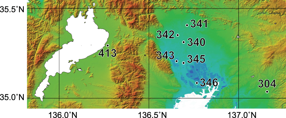
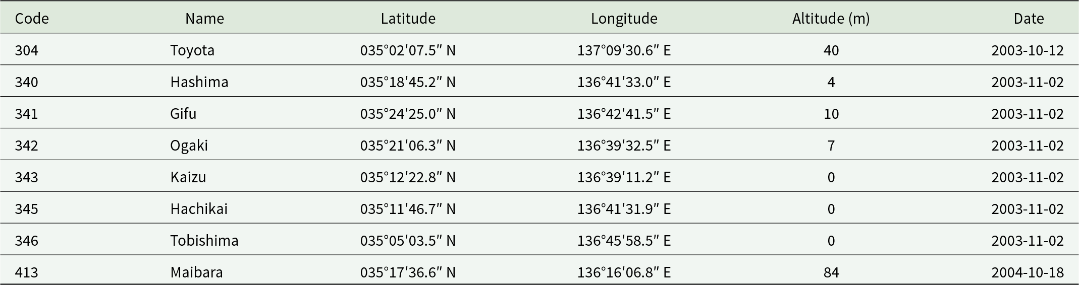
We collected Orius individuals in the fall of 2003–2004 from tall goldenrod (Solidago altissima) flowers at eight sites in Central Japan (fig. 1, table 1). Sampling was conducted in areas where both O. strigicollis and O. sauteri were distributed to compare these two species. Individuals were beaten off their flowers, dropped into plastic bags, and sucked using aspirators. Subsequently, the samples were preserved in a freezer until DNA analysis, after which they were transported to the laboratory.
Map which indicates the collection sites of the filed populations.

Figure 1 Long description
The map of Central Japan is a shaded-relief topographic map displaying collection sites marked with numeric labels. The map covers coordinates from 35.0°N to 35.5°N latitude and 136.0°E to 137.0°E longitude, with north oriented at the top. It features elevation and bathymetry coloring, where green indicates lower elevations, brown represents higher elevations and blue denotes water bodies. Key numeric labels include 413, 341, 342, 340, 343, 345, 346 and 304, indicating specific collection sites. The large water body in the west is Lake Biwa, with sites 413 and 342 clustered nearby. Sites 340, 341, 343, 345 and 346 are distributed eastward, with site 304 located further east. The map's purpose is to indicate collection sites for field populations, focusing on areas around Lake Biwa and extending eastward. The spatial pattern shows clustering near the lake and dispersal towards the east, highlighting the geographic scope and key features.
Collection records of the field populations of Orius sauteri and O. strigicollis used in this study

Table 1 Long description
The table lists eight field population collection records, giving a site code, place name, latitude and longitude, altitude in meters, and collection date. Seven of the eight sites are clustered around 35 degrees north latitude and 136 to 137 degrees east longitude. Most samples were collected on 2003-11-02 at Hashima, Gifu, Ogaki, Kaizu, Hachikai, Tobishima, and Maibara, indicating a single main sampling day. Toyota is the only site collected earlier, on 2003-10-12. Altitudes are low overall, ranging from 0 meters at Kaizu, Hachikai, and Tobishima up to 84 meters at Maibara, with Toyota at 40 meters. The lowest elevation sites are coastal or near sea level, while Maibara is the highest among the listed locations. The table provides locations and timing only and does not include counts or species-specific outcomes, so it cannot by itself indicate population size or composition.
Species identification
Genomic DNA was extracted from the whole body of each adult specimen using a Wizard genomic DNA purification kit (Promega, Tokyo, Japan). Each individual was homogenised in 100 µL of the supplied cell lysis solution in a 1.5 mL microtube, and DNA was isolated according to the manufacturer’s instructions. The DNA was subsequently dissolved in 100 µL of 1 mM Tris and 0.1 mM ethylenediaminetetraacetic acid (EDTA) buffer (TE) and stored at 4°C until analysis using polymerase chain reaction (PCR).
Multiplex PCR (Hinomoto et al., Reference Hinomoto, Muraji, Noda, Shimizu and Kawasaki2004) was conducted to identify the species of each individual. This method uses five primers to simultaneously amplify the internal transcribed spacer 1 of the ribosomal DNA and produces a species-specific banding pattern in agarose gel electrophoresis. PCR reactions were prepared in a final volume of 12.5 µL, containing 6.25 µL of 2 × Ex Premier DNA Polymerase (TaKaRa Bio, Shiga, Japan), 0.2 µM of each universal primer, 0.1 µM of each species-specific primer, and 0.5 µL of DNA template. PCR cycling conditions were: 94°C for 1 min; 30 cycles of 98°C for 10 s, 58°C for 15 s, and 68°C for 30 s. Products were separated on a 1.6% agarose gel using 40 mM Tris-acetate, 1 mM EDTA (TAE) buffer and visualised using GelRed (FUJIFILM Wako, Osaka, Japan) solution diluted 10,000-fold with TAE. Molecular weight standards in the form of a 200 bp DNA Ladder (TaKaRa Bio, Shiga, Japan) were run along with the samples.
Microsatellite
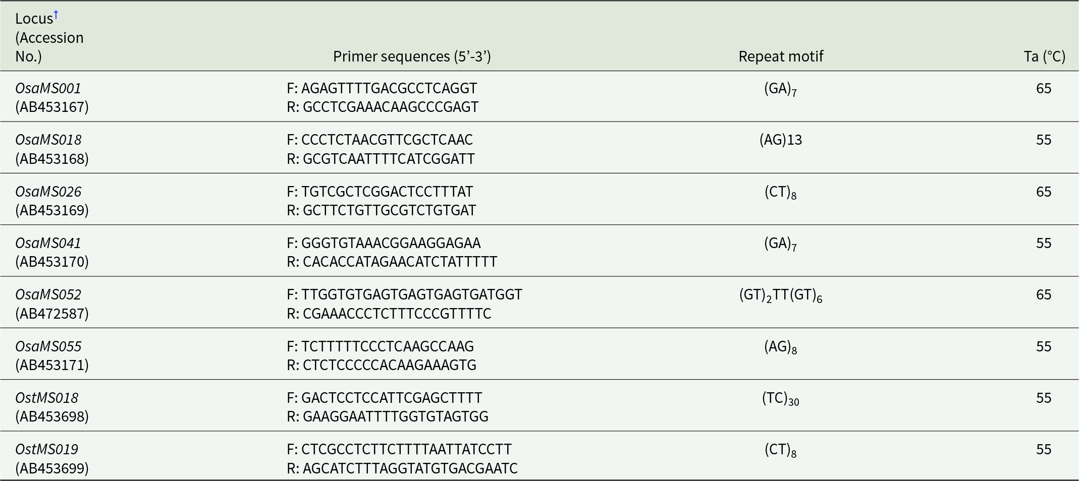
We utilised eight highly polymorphic microsatellite markers linked to species of the genus Orius (Hinomoto et al., Reference Hinomoto, Higaki and Noda2009) (table 2). These markers have been validated in previous studies and are highly diverse in O. strigicollis and O. sauteri (Hinomoto et al., Reference Hinomoto, Higaki and Noda2009).
Characteristics of eight microsatellite loci isolated from Orius strigicollis and O. sauteri, with primer sequences and annealing temperatures (Ta) (Hinomoto et al., Reference Hinomoto, Higaki and Noda2009)

Table 2 Long description
The table lists eight microsatellite loci from two Orius species, giving each locus name with accession number, forward and reverse primer sequences, the repeat motif, and the PCR annealing temperature in degrees C. Five loci use an annealing temperature of 55 degrees C and three use 65 degrees C. Repeat motifs vary in type and length, including GA, AG, CT, TC, and a compound GT motif. The longest repeat is OstMS018 with a TC repeat of length 30, while several loci have shorter repeats such as GA length 7 and CT length 8. The compound motif appears at OsaMS052, combining a short GT repeat, a TT interruption, and a longer GT repeat. Loci labeled OsaMS and OstMS correspond to different source species, but the table does not provide performance metrics such as polymorphism or amplification success, so comparisons are limited to primer design, motif, and annealing temperature.
† Note: OsaMS and OstMS indicate the loci isolated from O. strigicollis and O. sauteri, respectively.
PCR reactions were prepared in a total volume of 10 µL, consisting of 0.5 µL of genomic DNA, 5 µL of 2 × Ex Premier buffer, and 0.2 µM each of forward and reverse primers. The thermal cycling conditions were: 94°C for 1 min; 30 cycles of 98°C for 10 s, 55–65°C for 15 s, and 68°C for 30 s; followed by a final extension at 72°C for 10 min. Table 2 lists the primer sequences and annealing temperatures. The resulting PCR solution was mixed with the fluorochrome FAM:VIC:NED:PET = 1:1:2:2. Subsequently, 0.5 µL of the solution was mixed with 0.3 µL of GeneScan 500 LIZ Size Standard (Thermo Fisher Scientific, Tokyo, Japan) and 10 µL of Hi-Di formamide (Thermo Fisher Scientific, Tokyo, Japan). The solution was placed in a capillary electrophoresis sequencer DS3000 (Hitachi High-Tech Corporation, Tokyo, Japan). The results were genotyped for each individual using the GeneMarker software (SoftGenetics, State College, PA, USA). Allelic information, allele frequencies, observed heterozygosity (H O), expected heterozygosity (H E), and fixation index (F IS) were calculated. Deviations from Hardy–Weinberg equilibrium and pairwise F ST values were analysed using Genepop version 4.7.5 (Rousset, Reference Rousset2008). IBD patterns were evaluated using the Mantel test with geographic and genetic distance matrices.
Results
Species comparison
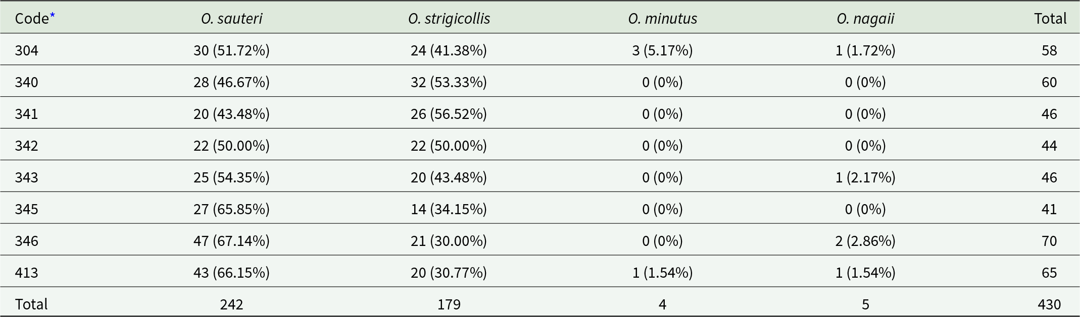
Table 3 shows the results of species identification using multiplex PCR. A total of 430 individuals from 8 populations were identified at the species level, including 242 O. sauteri, 179 O. strigicollis, 4 O. minutus, and 5 O. nagaii. Orius strigicollis and O. sauteri were approximately equal in number.
Species composition of the Orius spp. for each sampling site

Table 3 Long description
The table reports counts and within-site percentages of four Orius species at eight sampling site codes, plus totals. Overall, O. sauteri is the dominant species with 242 of 430 individuals, while O. strigicollis is second with 179; O. minutus and O. nagaii are uncommon with 4 and 5 individuals. Site totals range from 41 at code 345 to 70 at code 346. O. sauteri is the majority at most sites, peaking at code 346 with 47 individuals and about two thirds of that site’s sample, and also high at code 345 with about two thirds. O. strigicollis leads at codes 340 and 341, where it makes up just over half of individuals. O. minutus appears only at codes 304 and 413, and O. nagaii appears only at codes 304, 343, 346, and 413, always at very low percentages. Percentages are calculated within each site, so comparisons of percentages should consider that site sample sizes differ.
* Note: Regarding codes, see table 1.
Genetic diversity in each population
OsaMS018 showed results at 400 bp in addition to the known range of 113–137 bp; therefore, we treated this fragment as a different locus, called OsaMS018(2), to be counted in the results.
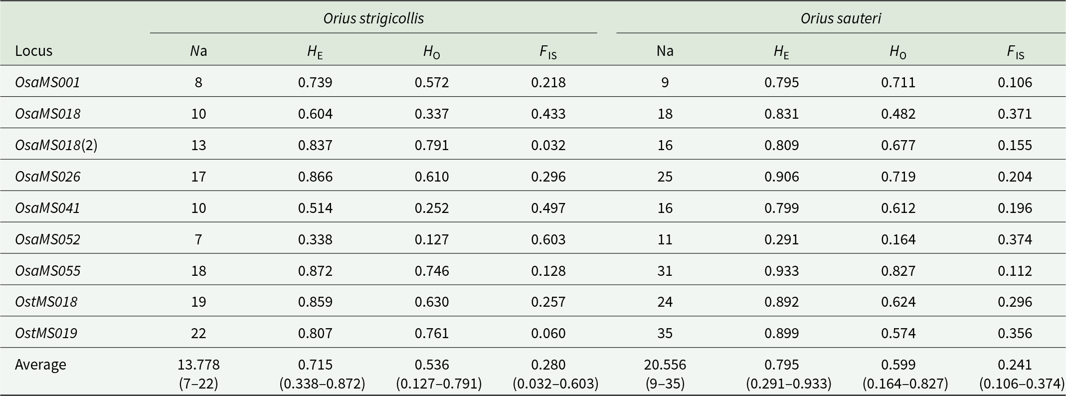
Table 4 reveals the genetic diversity parameters of the nine microsatellite loci in eight populations. For O. sauteri, the mean number of alleles (N a) for each locus, mean expected heterozygosity (H E), mean observed heterozygosity (H O), and mean inbreeding coefficient (F IS) were 20.556, 0.795, 0.599, and 0.241, respectively. The mean number of alleles (N a) for each locus, the mean expected heterozygosity (H E), the mean observed heterozygosity (H O), and the mean expected heterozygosity (F IS) were 13.778, 0.715, 0.536, and 0.28, respectively, for O. strigicollis.
Genetic diversity of the 9 microsatellite loci in 8 populations

Table 4 Long description
The table reports genetic diversity metrics for nine microsatellite loci in two species, listing number of alleles, expected heterozygosity, observed heterozygosity, and an inbreeding coefficient for each locus. Across loci, Orius sauteri generally has more alleles than Orius strigicollis, ranging from 9 to 35 versus 7 to 22, with the highest counts at OstMS019 in both species. Expected heterozygosity is typically higher in Orius sauteri, reaching 0.933 at OsaMS055, while Orius strigicollis peaks at 0.872 at OsaMS055. Observed heterozygosity varies by locus and is often lower than expected in both species; for example, Orius strigicollis is 0.127 at OsaMS052 and 0.791 at OsaMS018(2), while Orius sauteri ranges from 0.164 at OsaMS052 to 0.827 at OsaMS055. The inbreeding coefficient is positive at every locus for both species, indicating a consistent heterozygote deficit, with the largest values at OsaMS052 for Orius strigicollis (0.603) and OsaMS018 for Orius sauteri (0.371). On average, Orius sauteri has higher allele number and expected heterozygosity (20.556 and 0.795) than Orius strigicollis (13.778 and 0.715), while average observed heterozygosity is closer (0.599 versus 0.536) and average inbreeding is slightly lower in Orius sauteri (0.241 versus 0.280). Interpretation should consider that values are locus-specific summaries and do not by themselves identify causes such as sampling effects, population structure, or selection.
Note: Na, Number of alleles; H E, expected heterozygosity; H O, observed heterozygosity; and F IS, inbreeding coefficient.
The genetic diversity of O. sauteri was relatively high. The mean number of alleles (N a) and expected heterozygosity (H E) were significantly higher than those of O. strigicollis, as confirmed via t-tests (p = 0.001 for N a; p = 0.060 for H E, respectively). Although the observed heterozygosity (H O) of O. sauteri was higher than that of O. strigicollis, the difference was not statistically significant (p = 0.271 and 0.359, respectively). However, the expected heterozygosity of both species remained relatively moderate, indicating that a certain degree of inbreeding may have existed in the population. Additionally, the inbreeding coefficient (F IS) did not significantly differ between the two species (p > 0.49), indicating similar levels of population structures.
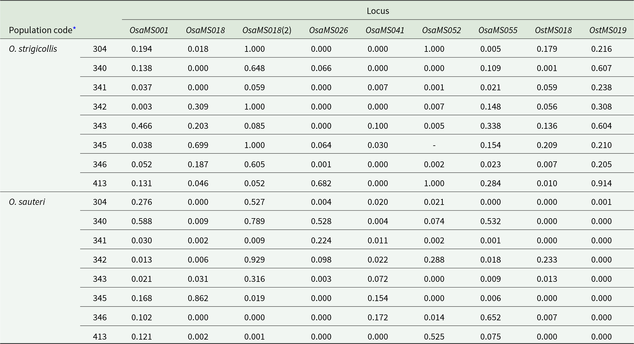
We performed Hardy–Weinberg equilibrium tests at nine microsatellite loci for two O. strigicollis and O. sauteri populations in central Japan (table 5). For the O. sauteri population, the p-values for all loci OsaMS001, OsaMS018, OsaMS018(2), OsaMS026, OsaMS041, OsaMS052, OsaMS055, OstMS018, and OstMS019 were <0.05, indicating that they did not conform to the Hardy–Weinberg equilibrium. Notably, loci OsaMS018, OsaMS018(2), and OstMS018 had extremely small p-values (p < 0.001), implying that the observed genotype frequencies at these three loci significantly deviated from the expected Hardy–Weinberg frequencies. Most of the loci in OsaMS018, OsaMS018(2), OsaMS026, OsaMS041, OsaMS052, OsaMS055, OstMS018, and OstMS019 showed p-values of <0.05 for O. strigicollis populations, suggesting that they also did not conform to the Hardy–Weinberg equilibrium. Particularly, loci OsaMS018, OsaMS018(2), and OsaMS041 demonstrated extremely low p-values (p < 0.001), implying that the observed genotype frequencies at these three loci significantly deviated from the expected Hardy–Weinberg ratios.
Hardy–Weinberg equilibrium test in each population of the Orius spp. in the Chubu region of Japan

Table 5 Long description
The table lists Hardy–Weinberg equilibrium test results (reported as p-values) for multiple microsatellite loci across population codes for two Orius species in Japan’s Chubu region. For O. strigicollis, several loci show very low values in many populations, especially OsaMS041 and OsaMS052 (often 0.000), while some loci reach 1.000 in specific populations (for example OsaMS026 in population 342 and OsaMS055 in population 304). O. strigicollis also has high values at OstMS019 in population 413 (0.914) and moderate to high values at OstMS018 in some populations (for example 0.209 in 345). For O. sauteri, many populations have values at or near 0.000 for OstMS018 and OstMS019, while some Osa loci show higher values in particular populations (for example OsaMS001 is 0.588 in 340 and OsaMS018 is 0.862 in 345). Across both species, results differ strongly by locus and population code, so any conclusion about equilibrium depends on the specific marker and sampling site. One cell is missing (shown as a dash) for O. strigicollis population 345 at OsaMS052, which limits comparisons for that locus in that population.
* Note: For population codes, see table 1.
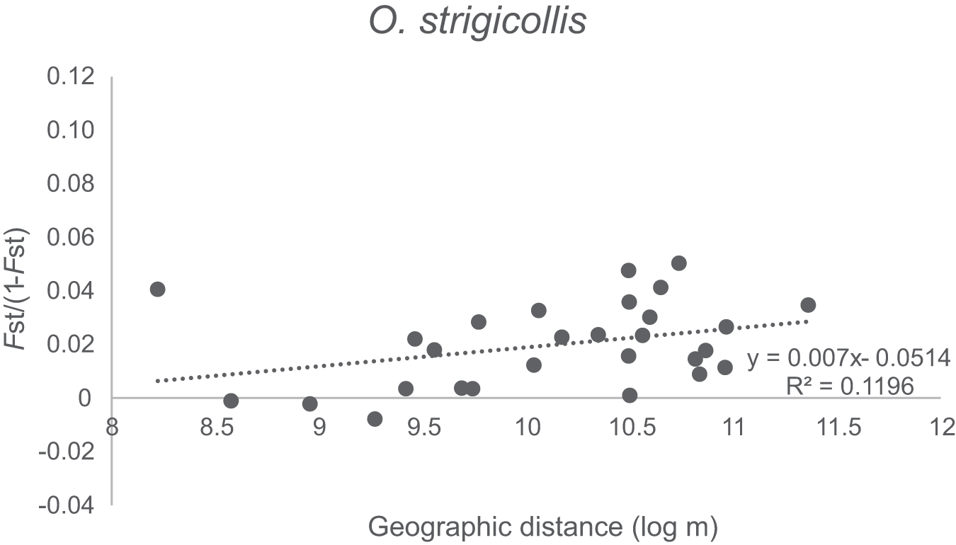
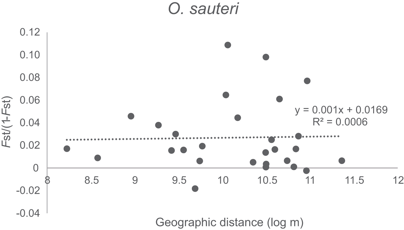
Furthermore, a significant positive correlation was observed between the geographic distance and pairwise-F ST in O. strigicollis (Spearman’s rank correlation, p = 0.04), indicating that genetic differentiation between populations increased with geographic distance (fig. 2). Additionally, no significant correlation was observed between distance and F ST in O. sauteri (p = 0.60) (fig. 3).
Regression analysis between the geographical and genetic distances among the eight Orius strigicollis populations in the Chubu region of Japan based on eight microsatellite loci. Positive correlation was noted (p = 0.04; one-tailed test).

Figure 2 Long description
O. strigicollis. The horizontal axis label is Geographic distance (log m). The horizontal axis range is 8 to 12. The vertical axis label is Fst over (1 minus Fst). The vertical axis range is negative 0.04 to 0.12. A dotted trend line is shown with the text y equals 0.007x minus 0.0514. The text R superscript 2 equals 0.1196 is shown. Scatter points are plotted across the graph, with points visible from about 8.2 to about 11.4 on the horizontal axis and from about negative 0.01 to about 0.05 on the vertical axis. A denser grouping of points appears around about 10 to 11 on the horizontal axis and about 0.01 to 0.04 on the vertical axis. A point appears near about 8.2 on the horizontal axis and about 0.04 on the vertical axis. No legend is shown.
Regression analysis between the genetic and geographical distances among the eight populations of Orius sauteri in the Chubu region of Japan based on eight microsatellite loci. No correlation was observed (p = 0.60; one-tailed test).

Figure 3 Long description
Scatter plot title: O. sauteri. The horizontal axis label is Geographic distance (log m). The horizontal axis shows tick labels 8, 8.5, 9, 9.5, 10, 10.5, 11, 11.5 and 12. The vertical axis label is Fst over (1 minus Fst). The vertical axis shows tick labels negative 0.04, negative 0.02, 0, 0.02, 0.04, 0.06, 0.08, 0.10 and 0.12. A dotted fitted line is drawn across the plot with the printed equation y equals 0.001x plus 0.0169 and R superscript 2 equals 0.0006. Points are plotted as filled circles. Many points lie between Geographic distance about 9.0 to 11.0 and Fst over (1 minus Fst) about 0 to 0.04. Several higher points appear around Fst over (1 minus Fst) about 0.06 to 0.11 near Geographic distance about 10.0 to 11.0. One point appears below 0 near Fst over (1 minus Fst) about negative 0.02 around Geographic distance about 9.7. No legend text is shown.
IBD
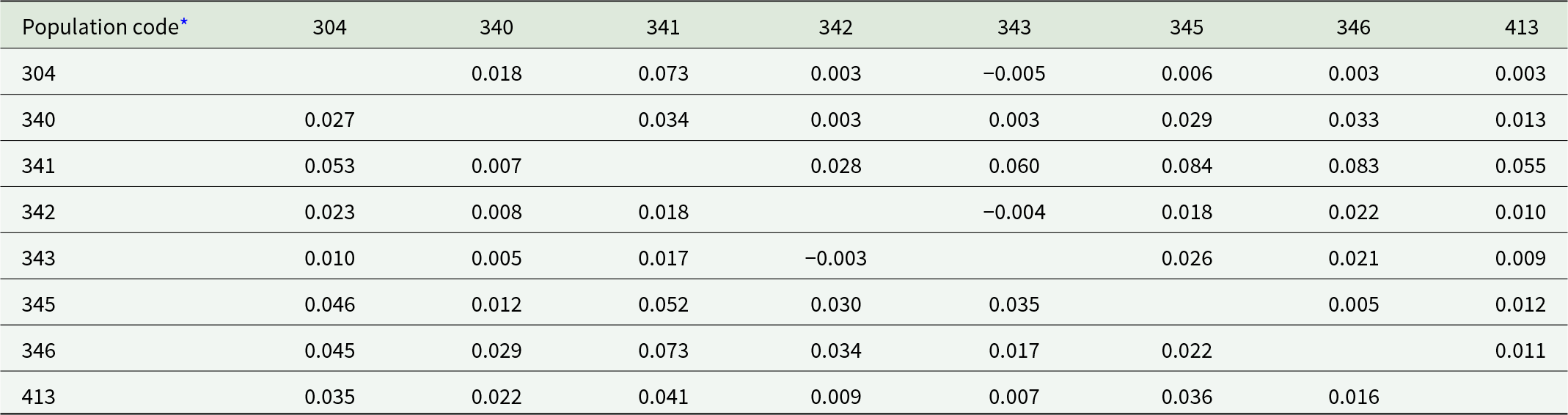
Based on the pairwise F ST values presented in table 6, genetic differentiation among O. strigicollis populations ranged from −0.003 to 0.073, indicating generally low levels of differentiation with a few population pairs exhibiting slightly higher divergence. Contrastingly, the O. sauteri populations revealed F ST values ranging from 0.003 to 0.084, suggesting a slightly broader range of genetic divergence. Thus, both species maintain relatively high levels of gene flow among populations, although O. sauteri tends to show slightly greater overall genetic structuring. No statistically significant difference was observed in the F ST values between the O. strigicollis and O. sauteri populations (Mann–Whitney U = 349.5, p = 0.811).
Pairwise F ST of Orius strigicollis (below diagonal) and Orius sauteri (above diagonal) among the 8 populations in the Chubu region of Japan

Table 6 Long description
The table reports pairwise FST values among eight population codes, with one species’ values in the upper-right half and the other species’ values in the lower-left half. Across both halves, most comparisons are small, indicating generally low genetic differentiation among populations. In the upper-right half, values range from −0.005 to 0.084, with the largest between 341 and 345 at 0.084 and other high values involving 341, such as 341 with 346 at 0.083 and 341 with 304 at 0.073. The smallest upper-right values include 304 with 343 at −0.005 and 342 with 343 at −0.004, with several near 0.003. In the lower-left half, values range from −0.003 to 0.073, with the largest between 341 and 346 at 0.073 and other relatively high values involving 341, such as 341 with 304 at 0.053 and 341 with 345 at 0.052. The smallest lower-left value is −0.003 between 343 and 342, and several other comparisons are near 0.005 to 0.013. Negative values can occur from sampling variation and should be interpreted as effectively no differentiation rather than true negative differentiation.
* Note: For population codes see table 1.
Discussion
This study compared the population genetic structures of O. strigicollis and O. sauteri in central Japan using microsatellite markers, with a special focus on IBD patterns. Although another congener, O. minutus, which is phylogenetically close relative to O. strigicollis (Honda et al., Reference Honda, Nakashima, Yanase, Kawarabata and Hirose1998), is also widely distributed in Japan, this species is mainly associated with arboreal habitats (Yasunaga, Reference Yasunaga1997; Hinomoto et al., Reference Hinomoto, Higaki and Noda2009). Since this study focuses on Orius populations associated with herbaceous vegetable crops (e.g. eggplant) in agricultural fields, we examined O. strigicollis and O. sauteri, which are the dominant species in these crop systems. A significant positive correlation between geographic distance and genetic differentiation (F ST) was detected in O. strigicollis, implying that limited dispersal and spatial separation contributed to the increased genetic divergence among the populations. Contrastingly, O. sauteri showed no significant IBD patterns, implying relatively higher gene flow and stronger population connectivity across its range.
The presence of an IBD pattern in O. strigicollis aligns with the theoretical expectation that species with restricted dispersal would demonstrate greater genetic differentiation in geographic space (Slatkin, Reference Slatkin1993; Rousset, Reference Rousset1997). Generally, IBD is pronounced in species with low dispersal abilities, small effective population sizes, and heterogeneous environments that create physical or ecological barriers to gene flow. Conversely, high dispersal ability, large population size, and habitat continuity tend to weaken or obscure IBD patterns (Broquet and Petit, Reference Broquet and Petit2009). Thus, our results imply that O. strigicollis is characterised by limited movement among its habitats, leading to greater spatial genetic structuring.
Contrastingly, O. sauteri maintains a relatively uniform genetic structure across various geographic locations, which is consistent with its higher gene flow and broader ecological adaptability. Species capable of dispersing over long distances or exploiting a wide range of habitats often show weak genetic differentiation across landscapes (Storfer et al., Reference Storfer, Murphy, Evans, Goldberg, Robinson, Spear, Dezzani, Delmelle, Vierling and Waits2007). The lack of an IBD pattern in O. sauteri may be due to its high mobility, large effective population size, and ability to occupy diverse environments, thereby decreasing the genetic effects of geographic separation.
These contrasting patterns between the two species provide crucial insights into how ecological and behavioural traits shape the population genetic structure. Particularly, differences in dispersal capabilities appear to be vital factors affecting the extent of genetic differentiation. Such knowledge is necessary for designing biological control strategies in which the enhancement and sustainability of indigenous natural enemy populations are prioritised (Eilenberg et al., Reference Eilenberg, Hajek and Lomer2001). Therefore, understanding natural dispersal dynamics is crucial.
From a practical standpoint, the higher genetic connectivity observed in O. sauteri suggests that this species may be more resilient to the alterations in the environment and more effective across broader geographical areas. Therefore, O. sauteri may be better suited for biological conservation control programs that rely on maintaining and improving naturally occurring populations without artificial augmentation. Contrastingly, O. strigicollis, with its stronger population structure and more sedentary activity, may necessitate region-specific management strategies, such as habitat enhancement targeted at local populations, to maximise biological control efficacy.
This study has several limitations. First, sampling was conducted during a limited time window, and temporal genetic variation could not be evaluated. Second, although microsatellite markers provided informative insights, the use of more genome-wide markers such as SNPs could enhance the resolution of population structure. Despite these limitations, our findings contribute valuable preliminary information on the genetic diversity and structure of Orius species in the studied region. Although this study provides valuable insights into the population genetics of O. strigicollis and O. sauteri, further studies are required to understand the ecological and environmental factors that affect their gene flow. Environmental heterogeneity, habitat fragmentation, and population density could all play roles in shaping these patterns. Future studies should incorporate broader geographic sampling and detailed ecological data and consider the use of high-resolution genomic techniques, such as whole-genome sequencing, to show fine-scale adaptive variation and dispersal barriers. Such efforts will contribute to optimising the use of Orius species for sustainable pest management strategies.
Acknowledgements
This work was partly supported by Cabinet Office, Government of Japan, Moonshot Research and Development Program for Agriculture, Forestry and Fisheries (funding agency: Bio-oriented Technology Research Advancement Institution) JPJ009237.
Competing interests
The authors declare no conflict of interest.
Ethical standards
Not applicable.