On the effective non-vanishing of Hecke–Maass L-functions at special points

Zhi Qi

doi:10.4153/S0008414X26102454

On the effective non-vanishing of Hecke–Maass L-functions at special points

Part of: Zeta and $L$-functions: analytic theory Discontinuous groups and automorphic forms

Published online by Cambridge University Press: 23 September 2026

Zhi Qi

Show author details

Zhi Qi*: Affiliation:
Zhejiang University , China
*: e-mail: zhi.qi@zju.edu.cn

Article contents

Abstract
Introduction
Kuznetsov trace formulas
Hecke–Maass L-functions
Analysis for the Bessel integrals
A useful unsmoothing lemma
Preliminaries
Setup
The twisted first moment
The twisted second moment
The mollified moments
Moments with no twist and smooth weight
Sums of variant Kloosterman sums
Further analysis for the Bessel integrals
The explicit formula
Proof of the density theorems
Proof of the non-vanishing results on the Riemann hypothesis
Footnotes
References

Rights & Permissions

Abstract

In this article, we consider the non-vanishing problem for the family of special Hecke–Maass L-values $ L (1/2+it_f, f) $ with $f (z)$ in an orthonormal basis of (even or odd) Hecke–Maass cusp forms of Laplace eigenvalue $1/4 + t_f^2$ ($t_f> 0$). We prove that 20% of $L (1/2+it_f, f)$ for $ t_f \leqslant T$ do not vanish as $T \rightarrow \infty $. For comparison, it is known that the non-vanishing proportion is at least 25% for the central L-values $L (1/2, f)$. Further, 20% may be raised to 50% conditionally on the generalized Riemann hypothesis. Moreover, we prove non-vanishing results on the short interval $|t_f-T| \leqslant T^{\mu }$ for any $0 < \mu < 1$.

Keywords

Maass forms L-functions Kuznetsov formula

MSC classification

Primary: 11F72: Spectral theory; Selberg trace formula 11M41: Other Dirichlet series and zeta functions

Information

Type: Article
Information: Canadian Journal of Mathematics , First View , pp. 1 - 41

DOI: https://doi.org/10.4153/S0008414X26102454 [Opens in a new window]
Copyright: © The Author(s), 2026. Published by Cambridge University Press on behalf of Canadian Mathematical Society

1 Introduction

1.1 Definitions

Let be an orthonormal basis of Hecke–Maass cusp forms on the modular surface $ \mathrm{SL}_2 (\mathbf{Z}) \backslash \mathbf{H} $ . Assume that each is either even or odd in the sense that $ f (-\overline {z}) = (-1)^{\delta _f} f (z)$ for $\delta _f = 0$ or $ 1$ . Let or be the subset of even or odd forms in respectively. 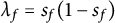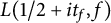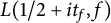For , let $\lambda _{f} = s_{f} (1-s_{f})$ be its Laplace eigenvalue, with $s_f = 1/2+ i t_f$ 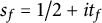( $t_f> 0$ ). The Fourier expansion of $f (z)$ reads

$$ \begin{align*} f (x+iy) = \sqrt{y} \sum_{n \neq 0} \rho_f (n) K_{i t_f} (2\pi |n| y) e (n x), \end{align*} $$

where, as usual, $K_{\nu } (x)$ is the K-Bessel function and $e (x) = \exp (2\pi i x)$ . Let $\lambda _f (n)$ ( $n \geqslant 1$ ) be the Hecke eigenvalues of $f (z)$ . It is well known that $\rho _f (\pm n) = \rho _f (\pm 1) \lambda _f (n) $ , while $\rho _f (-1) = (-1)^{\delta _f} \rho _f (1)$ . Define the harmonic weight

$$ \begin{align*} \omega_f = \frac {|\rho_f (1)|^2} {\cosh \pi t_f}. \end{align*} $$ omega Subscript f Baseline equals StartFraction StartAbsoluteValue rho Subscript f Baseline left parenthesis 1 right parenthesis EndAbsoluteValue squared Over hyperbolic cosine pi t Subscript f Baseline EndFraction period

The Hecke–Maass L-function of $f (z)$ is defined by

$$ \begin{align*} L (s, f) = \sum_{n =1}^{\infty}\frac{ \lambda_f (n) }{n^s} , \end{align*} $$ upper L left parenthesis s comma f right parenthesis equals sigma summation Underscript n equals 1 Overscript infinity Endscripts StartFraction lamda Subscript f Baseline left parenthesis n right parenthesis Over n Superscript s Baseline EndFraction comma

for $\mathrm {Re} (s)> 1$ , and by analytic continuation on the whole complex plane.

1.2 Effective non-vanishing results

As the motivation of this article, the author [Reference QiQi] recently established an effective refinement (recorded below) of the non-vanishing result of Luo [Reference LuoLuo3] for the Rankin–Selberg special L-values $L (s_f, Q \otimes f)$ . The non-vanishing condition for $L (s_f, Q \otimes f)$ arises in the Phillips–Sarnak deformation theory of Maass cusp forms [Reference Phillips and SarnakPS] and was studied by Deshouillers, Iwaniec, and Luo [Reference Deshouillers and IwaniecDI, Reference LuoLuo1, Reference LuoLuo3, Reference LuoLuo4].

Theorem [Reference QiQi]

Let $Q (z)$ be a fixed holomorphic cusp newform of even weight $2k$ and square-free level q. Let $3/4 < \mu < 1$ . We have

(1.1)

$lim inf as T approaches infinity of the fraction with numerator # { f in B : t sub f <= T, L(s sub f, Q tensor f) != 0 } all over denominator # { f in B : t sub f <= T } is greater than or equal to gamma(Q) all over 11.$

(1.2)

$lim inf as T approaches infinity of the fraction with numerator # { f in B : |t sub f - T| <= T^mu, L(s sub f, Q tensor f) != 0 } all over denominator # { f in B : |t sub f - T| <= T^mu } >= gamma(Q) times fraction 4mu - 3 all over 4mu + 7.$

where $\gamma (Q )$ is the Euler product:

(1.3) $$ \begin{align} \begin{aligned} \prod_{p \nmid q} \bigg(1 - \frac {a(p)^2} {p(p+1) } \bigg)^{-1} \bigg(1 + \frac {a(p)^2} {p+1 } \bigg) \bigg( 1 - \frac {a(p)^2 - 2} {p} + \frac 1 {p^2} \bigg) \bigg( 1 - \frac {1} { p } \bigg)^2 \cdot \prod_{p | q} \bigg( 1 - \frac 1 {p^2 } \bigg) , \end{aligned} \end{align} $$

with $a (p)$ the p-th Hecke eigenvalue of $Q (z)$ .

It is natural to consider the more fundamental family of Hecke–Maass L-functions $L (s, f)$ and to see how large a non-vanishing proportion at $s = s_f$ one might attain. It is also interesting to compare our non-vanishing results for $L (s_f, f)$ with those for central L-values $L(1/2, f)$ , with or without the Riemann hypothesis.

To be explicit, our main theorems for the non-vanishing statistic of the special L-values $L (s_f, f)$ are as follows.

Theorem 1 We have

(1.4)

$lim inf as T approaches infinity of the fraction with numerator # { f in B sub delta : t sub f <= T, L(s sub f, f) != 0 } all over denominator # { f in B sub delta : t sub f <= T } is greater than or equal to 2 all over pi-squared$

for $\delta = 0, 1$ ; (1.4) is also valid for the full family .

On the long interval $t_f \leqslant T$ , Theorem 1 manifests that at least $2 / \pi ^2 \approx 20 \%$ of the special L-values $L (s_f, f) $ do not vanish for , while it is proven in [Reference Balkanova, Huang and SödergrenBHS, Reference Liu and QiLQ2] that 25% of the central L-values $L(1/2, f)$ do not vanish for , although, in the latter case, $L (1/2, f) = 0$ 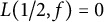trivially on the whole odd sub-basis as the root number $\epsilon _f = - 1$ .

Theorem 2 Let $ 0 < \mu < 1$ . We have

(1.5)

$lim inf as T approaches infinity of the fraction with numerator # { f in B sub delta : | t sub f - T | <= T super mu , L ( s sub f , f ) != 0 } all over denominator # { f in B sub delta : | t sub f - T | <= T super mu } >= 6 / pi^2 min { 1/3 , mu / ( mu + 1 ) }.$

This is an effective refinement of the result of Xu [Reference XuXu] in which he proved that (on the even sub-basis ) the ratio in (1.5) is bounded below by an unexplicit constant as $T \rightarrow \infty $ .

Theorem 3 Assume the Riemann hypothesis for every $L (s, f)$ with and for all Dirichlet L-functions (including the Riemann zeta function). Then,

(1.6)

$lim inf as T approaches infinity of the fraction with numerator # { f in B delta : t f <= T, L(s f, f) != 0 } all over denominator # { f in B delta : t f <= T } is greater than or equal to 1/2.$

Thus, on the Riemann hypothesis, for the non-vanishing percentage 20% for $ L (s_f, f) $ is raised drastically to 50%, but 25% for $L(1/2, f)$ is raised only to 28% (see Corollary A.1).

Theorem 4 Assume the Riemann hypothesis as in Theorem 3. Then,

(1.7)

$lim inf as T approaches infinity of the fraction with numerator # {f in B sub delta : |t sub f - T| <= T^mu, L(s sub f, f) != 0} all over denominator # {f in B sub delta : |t sub f - T| <= T^mu} >= min {mu / (mu + 1), (3mu - 1) / 3mu}.$

These conditional results will be deduced from the extended density theorem for $L (s, f)$ at $s = s_f$ .

Figure 1:

A comparison of the proportions in (1.5) and (1.7).

A line graph comparing two non-vanishing proportions across a horizontal axis labeled mu from 0 to 1. See long description.

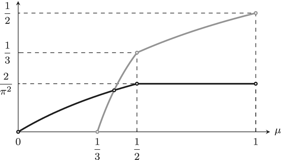
Figure 1. Long description

A line graph with a horizontal axis labeled mu and a vertical axis with fractional values. The horizontal axis has tick marks at 0, 1 over 3, 1 over 2, and 1. The vertical axis has tick marks at 2 over pi-squared, 1 over 3, and 1 over 2.

Two lines are plotted:

* A black line starts at the origin (0,0) and follows a concave curve upward until it reaches the point (1 over 2, 2 over pi-squared). From that point, it continues as a horizontal flat line to the right until mu equals 1.

* A grey line starts on the horizontal axis at (1 over 3, 0). It rises steeply in a linear fashion, intersecting the black line before reaching a vertex at (1 over 2, 1 over 3). From there, it continues to rise with a shallower linear slope until it terminates at the point (1, 1 over 2).

Horizontal and vertical dashed grid lines connect the key vertices of both plots to their respective values on the axes.

1.3 Twisted spectral moments

Our proof of Theorems 1 and 2 will rely on the asymptotic formulas for the twisted first and second moments of $ L (s_f , f ) $ .

Let $T, \varPi $ be large parameters such that $T^{\varepsilon } \leqslant \varPi \leqslant T^{1-\varepsilon }$ . Define the smoothly weighted twisted moments on the (even or odd) cuspidal spectrum:

(1.8)

(1.9)

Theorem 5 Let the notation be as above. We have

(1.10)

where $\delta (m ,1)$ is the Kronecker $\delta $ that detects $m = 1$ .

Theorem 6 Let the notation be as above. Assume that $m_1, m_2 < \varPi ^{1-\varepsilon }$ . Set

(1.11) $$ \begin{align} m = (m_1, m_2), \qquad r = \frac {m_1m_2} {m^2}. \end{align} $$

Then,

(1.12)

C sub 2 super delta (m sub 1, m sub 2) = Pi T all over pi square root of pi r times ( (log T over r + gamma sub delta) sigma sub -1 (m) - 2 sigma prime sub -1 (m) + O sub epsilon (T super epsilon (Pi square root of T + T over square root of r + Pi cubed over T square root of r) ) )

where

(1.13) $$ \begin{align} \gamma_{0 } = \gamma - \log 8 \pi^2 - \frac {\pi} 2 , \qquad \gamma_1 = \gamma - \log 8 \pi^2 + \frac {\pi} 2, \end{align} $$

with $\gamma $ the Euler constant, and

(1.14) $$ \begin{align} \sigma_{-1} ( m ) = {\sum_{d | m } } \frac {1} {d }, \qquad \sigma_{-1}' ( m ) = {\sum_{d | m } } \frac {\log d } {d }. \end{align} $$ StartLayout 1st Row sigma Subscript negative 1 Baseline left parenthesis m right parenthesis equals sigma summation Underscript d vertical bar m Endscripts StartFraction 1 Over d EndFraction comma sigma prime Subscript negative 1 Baseline left parenthesis m right parenthesis equals sigma summation Underscript d vertical bar m Endscripts StartFraction log d Over d EndFraction period EndLayout

Corollary 7 Let $T^{\varepsilon } \leqslant \varPi \leqslant T^{1-\varepsilon }$ . We have

(1.15)

(1.16)

Corollary 8 We have

(1.17) $$ \begin{align} \sideset{}{^{\delta}}\sum_{ t_f \leqslant T} \omega_f L (s_f, f ) = \frac {T^{2}} {2 \pi^2} + O_{ \varepsilon } \big(T^{3/2+\varepsilon }\big), \end{align} $$

(1.18) $$ \begin{align} \sideset{}{^{\delta}}\sum_{ t_f \leqslant T} \omega_f |L (s_f, f )|^2 = \frac {1 } {2 \pi^2} T^2 \log T + \frac {2\gamma_{\delta} - 1 } {4 \pi^2 } T^2 + O_{ \varepsilon } \big(T^{3/2+\varepsilon }\big), \end{align} $$

where the superscript $\delta $ indicates summation over .

1.4 Density theorems

Our proof of Theorems 3 and 4 will rely on the extended density theorem under the Riemann hypothesis for Dirichlet L-functions.

Let us denote the non-trivial zeros of $L (s, f)$ by

$$ \begin{align*}\rho_f = \frac 1 2 + i \gamma_f;\end{align*} $$

if the generalized Riemann hypothesis for $L (s, f)$ is assumed, then $\gamma _f$ are all real.

Definition 1.1 Define the $1$ -level density of $L (s, f)$ at $s_f = 1/2+ it_f$ 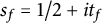to be

(1.19) $$ \begin{align} D (f; \unicode{x3c6}; T) = \sum_{\gamma_f} \unicode{x3c6} \bigg(\frac {\log T} {2\pi} (\gamma_f - t_f) \bigg) , \end{align} $$ upper D left parenthesis f semicolon phi semicolon upper T right parenthesis equals sigma summation Underscript gamma Subscript f Baseline Endscripts phi left parenthesis StartFraction log upper T Over 2 pi EndFraction left parenthesis gamma Subscript f Baseline minus t Subscript f Baseline right parenthesis right parenthesis comma

where T is a large scaling parameter and $\unicode{x3c6} : \mathbf {R} \rightarrow \mathbf {C}$ is an even Schwartz function such that its Fourier transform

$$ \begin{align*} \hat{\unicode{x3c6}} (y) = \int_{-\infty}^{\infty} \unicode{x3c6} (x) e (-xy) \mathrm{d} x \end{align*} $$

has compact support.

For $T, \varPi $ as above, define the smoothly averaged $1$ -level density

(1.20)

Theorem 9 Let the notation be as above. Assume the Riemann hypothesis (for the Riemann zeta function). Then, for $\hat {\unicode{x3c6} }$ of support in $(-1, 1)$ , we have

(1.21)

for any fixed $0 < \mu < 1$ .

Recall that $W (\mathrm {U}) (x) \equiv 1$ according to Katz and Sarnak [Reference Katz and SarnakKS].

Theorem 9 manifests that the symmetry types of $ L (s_f , f) $ on and are both unitary, while it is proven in [Reference Liu and QiLQ1, Appendix] that the symmetry types of $ L (1/2 , f) $ on and are orthogonal of different parity: $\mathrm {SO} (\mathrm {even})$ and $\mathrm {SO} (\mathrm {odd})$ , respectively. Note that for $\hat {\unicode{x3c6} }$ of support in $(-1, 1),$ one is unable to differentiate $\mathrm {SO} (\mathrm {even})$ and $\mathrm {SO} (\mathrm {odd})$ .

However, in order to obtain a non-trivial non-vanishing result for $ L (s_f , f) $ (as in Theorems 3 and 4), we must let the support of $ \hat {\unicode{x3c6} } $ go beyond $[-1, 1]$ as in the following extended density theorem.

Theorem 10 Define $v (\mu ) = \min \{ 3\mu , 1 + \mu \}$ . Then, for $1/3 < \mu < 1$ , we have

(1.22)

for $\hat {\unicode{x3c6} }$ of support in $(-v (\mu ) , v(\mu ) )$ if we assume, in addition, the Riemann hypothesis for Dirichlet L-functions.

Remark 1.1 We have the smoothly weighted harmonic Weyl law (see (2.13)):

(1.23)

Remark 1.2 Note that in Theorems 9 and 10, there is no need to assume the Riemann hypothesis for $L(s, f)$ since the definition in (1.19) makes sense even if $\gamma _f$ are not real as $\unicode{x3c6} $ is entire.

Notation

By or $X = O (Y),$ we mean that $|X| \leqslant c Y$ for some constant ${c> 0}$ , and by $X \asymp Y,$ we mean that and . We write 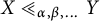or $ {X = O_{\alpha , \beta , \ldots } (Y)} $ if the implied constant c depends on $\alpha $ , $\beta $ , $\ldots $ .

By “negligibly small,” we mean $ O_A ( T^{-A} )$ for arbitrarily large but fixed $A $ .

The notation $x \sim X$ stands for $ X \leqslant x \leqslant 2 X $ .

Throughout the article, $\varepsilon $ is arbitrarily small and its value may differ from one occurrence to another.

2 Kuznetsov trace formulas

Let $h (t)$ be an even function satisfying the conditions:

(i) $h (t)$ is holomorphic in $|\mathrm {Im}(t)|\leqslant {1}/{2}+\varepsilon $ ;
(ii) in the above strip.

For $m, n \geqslant 1$ , define the cuspidal term

(2.1)

and the Eisenstein term

(2.2) $$ \begin{align} \Xi (m, n ) = \frac{1}{\pi} \int_{-\infty}^{\infty} \omega(t) h(t) \tau_{it}(m) \tau_{it} (n) \mathrm{d} t, \end{align} $$

where $\omega _f$ and $\lambda _{f} (n)$ are defined before in Section 1.1, and

(2.3) $$ \begin{align} \omega (t) = \frac {1 } {|\zeta (1 + 2it)|^2} , \qquad \tau_{\nu } (n) = \sum_{ a b = n} (a/b)^{ \nu }. \end{align} $$

On the other hand, define the Plancherel integral

(2.4) $$ \begin{align} H = \frac {1} { \pi^2} \int_{-\infty}^{\infty} h(t) { \tanh (\pi t) t \mathrm{d} t } , \end{align} $$

and the Kloosterman–Bessel sum

(2.5) $$ \begin{align} \mathrm{KB}^{ \pm} (m, n ) = \sum_{ c = 1 }^{\infty} \frac {S ( m , \pm n; c)} { c} H^{ \pm} \bigg( \frac {4\pi \textstyle \sqrt { m n } } { c} \bigg), \end{align} $$

where $S (m, \pm n; c)$ is the Kloosterman sum and $H^{\pm } (x)$ are the Bessel integrals

(2.6) $$ \begin{align} H^{ +} (x) &= \frac {2 i} {\pi} \int_{-\infty}^{\infty} h(t) J_{2it} ( x) \frac {t \mathrm{d} t } {\cosh (\pi t)},\end{align} $$

(2.7) $$ \begin{align} H^{ -} (x) &= \frac 4 {\pi^2 } \int_{-\infty}^{\infty} h(t) K_{2it} ( x) {\sinh (\pi t)} t \mathrm{d} t. \end{align} $$

By [Reference WatsonWat, Formula 3.7 (6)],

$$ \begin{align*}2 K_{\nu } (z) = \pi \frac {I_{-\nu } (z) - I_{\nu } (z)} {\sin (\pi \nu )} ,\end{align*} $$ StartLayout 1st Row 2 upper K Subscript nu Baseline left parenthesis z right parenthesis equals pi StartFraction upper I Subscript negative nu Baseline left parenthesis z right parenthesis minus upper I Subscript nu Baseline left parenthesis z right parenthesis Over sine left parenthesis pi nu right parenthesis EndFraction comma EndLayout

where $I_{\nu } (z)$ is the I-Bessel function. Hence, we may rewrite (2.7) in a form which is similar to (2.6):

(2.8) $$ \begin{align} H^{ -} (x) = \frac {2 i} {\pi} \int_{-\infty}^{\infty} h(t) I_{2it} ( x) \frac {t \mathrm{d} t } {\cosh (\pi t)}. \end{align} $$

The Kuznetsov trace formula for the even or odd cusp forms reads (see [Reference Conrey and IwaniecCI, Section 3]):

(2.9) $$ \begin{align} 2 \Delta_{ \delta } (m, n ) + 2 (1-\delta) \Xi (m, n) = \delta (m, n) H + \mathrm{KB}^{ +} (m, n) + (-1)^{\delta} \mathrm{KB}^{ -} (m, n) , \end{align} $$

where $\delta (m, n)$ is the Kronecker $\delta $ -symbol.

2.1 The Kloosterman sum

Recall that

(2.10) $$ \begin{align} S (m, n; c ) = \sideset{}{^\star}\sum_{ \alpha (\mathrm{mod} \, c) } e \bigg( \frac { \alpha m + \overline{\alpha } n} {c} \bigg) , \end{align} $$ StartLayout 1st Row upper S left parenthesis m comma n semicolon c right parenthesis equals sigma summation Superscript star Baseline Underscript alpha left parenthesis mod c right parenthesis Endscripts e left parenthesis StartFraction alpha m plus ModifyingAbove alpha With quotation dash n Over c EndFraction right parenthesis comma EndLayout

where the $\star $ indicates the condition $(\alpha , c) = 1$ and $ \overline {\alpha }$ is given by $\alpha \overline {\alpha } \equiv 1 (\mathrm {mod} \, c)$ . We have the Weil bound:

(2.11)

where, as usual, $\tau (c) = \tau _0 (c) $ 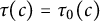is the number of divisors of c.

2.2 The Hecke relation

We have

(2.12) $$ \begin{align} \lambda_f (m) \lambda_f (n) = \sum_{d | (m, n)} \lambda_f (mn/d^2), \qquad \tau_{\nu } (m) \tau_{\nu } (n) = \sum_{d | (m, n)} \tau_{\nu } (mn/d^2). \end{align} $$

2.3 The Weyl law

Finally, we record here the harmonic-weighted Weyl law for :

(2.13)

By the method in [Reference LiLi2], this follows from the Kuznetsov trace formula for .

3 Hecke–Maass L-functions

For , define

(3.1) $$ \begin{align} L (s, f) = \sum_{n =1}^{\infty}\frac{ \lambda_f (n) }{n^s} , \end{align} $$ upper L left parenthesis s comma f right parenthesis equals sigma summation Underscript n equals 1 Overscript infinity Endscripts StartFraction lamda Subscript f Baseline left parenthesis n right parenthesis Over n Superscript s Baseline EndFraction comma

for $\mathrm {Re} (s)> 1$ . It is known that $L (s, f)$ has analytic continuation to the whole complex plane and satisfies the functional equation

(3.2) $$ \begin{align} \Lambda (s, f) = \epsilon_f \Lambda (1-s, f), \qquad \epsilon_f = (-1)^{\delta_f} , \end{align} $$

with

(3.3) $$ \begin{align} \Lambda (s, f) = \Gamma_{\mathbf{R}}^{\delta_f} (s - it_f) \Gamma_{\mathbf{R}}^{\delta_f} (s + it_f) L (s, f) , \end{align} $$

where

(3.4) $$ \begin{align} \Gamma_{\mathbf{R}}^{\delta} (s) = \pi^{-s/2} \Gamma ((s+\delta) /2). \end{align} $$

Note that, in parallel to (3.1), if we replace $\lambda _f (n)$ by $ \tau _{ it} (n) $ as defined in (2.3), then

(3.5) $$ \begin{align} \zeta (s -it ) \zeta (s + it ) = \sum_{n =1}^{\infty}\frac{ \tau_{it} (n )}{n^{s }}. \end{align} $$ zeta left parenthesis s minus i t right parenthesis zeta left parenthesis s plus i t right parenthesis equals sigma summation Underscript n equals 1 Overscript infinity Endscripts StartFraction tau Subscript i t Baseline left parenthesis n right parenthesis Over n Superscript s Baseline EndFraction period

Moreover, we have the Euler factorization

(3.6) $$ \begin{align} L (s, f) = \prod_{p} \bigg( 1 - \frac {\alpha_f (p)} {p^s} \bigg)^{-1} \bigg( 1 - \frac {\beta_f (p)} {p^s} \bigg)^{-1} , \end{align} $$

for $\mathrm {Re} (s)> 1$ , and the Kim–Sarnak bound [Reference KimKim]

(3.7) $$ \begin{align} |\alpha_f (p) |, \, |\beta_f (p) | \leqslant p^{\frac 7 {64}}. \end{align} $$

4 Analysis for the Bessel integrals

Let $T, \varPi $ be large parameters with $ T^{\varepsilon } \leqslant \varPi \leqslant T^{1-\varepsilon } $ . In this section, we consider the Bessel transforms of test functions in the form

(4.1) $$ \begin{align} h (t; y) = \unicode{x3b3} (t) y^{-2it} \unicode{x3D5} (t) + \unicode{x3b3} (- t) y^{2it} \unicode{x3D5} (- t), \end{align} $$

for $\unicode{x3b3} (t) $ in the function space $ \mathscr {Q}_{\kappa } $ or $ \mathscr {T}_{\tau } $ defined below in Definitions 4.1 or 4.2, and

(4.2) $$ \begin{align} \unicode{x3D5} (t) = \exp \bigg( \! - \frac {(t - T)^2 } {\varPi^2 } \bigg). \end{align} $$ normal phi left parenthesis t right parenthesis equals exp left parenthesis minus StartFraction left parenthesis t minus upper T right parenthesis squared Over upper Pi squared EndFraction right parenthesis period

In the case that $\unicode{x3b3} (t)$ is even, we also need to consider

(4.3) $$ \begin{align} h_2 (t; y) = h (t; y) + h (t; 1/y) = 2 \unicode{x3b3} (t) \cos (2 t \log y) (\unicode{x3D5} (t) + \unicode{x3D5} (-t)). \end{align} $$

Let $H^{\pm } (x, y)$ and $H^{\pm }_2 (x, y)$ denote the Bessel transforms of $h (t; y)$ and $ h_2 (t; y) $ as in (2.6) and (2.7) or (2.8). Note that

(4.4) $$ \begin{align} H_2^{\pm} (x, y) = H^{\pm} (x, y) + H^{\pm} (x, 1/y), \end{align} $$

so the results below for $H^{\pm } (x, y) $ will be valid for $H^{\pm }_2 (x, y) $ as well.

Definition 4.1 For fixed real $\kappa $ , let $ \mathscr {Q }_{\kappa } $ denote the space of holomorphic functions $\unicode{x3b3} (t) $ on the strip $ |\mathrm {Im} (t)| \leqslant 1/2 + \varepsilon $ such that

(4.5)

Definition 4.2 For fixed real $\tau $ , let $ \mathscr {T }_{\tau } \subset C^{\infty } (\mathbf {R})$ 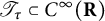denote the space of smooth functions on $ \mathbf {R} $ such that

(4.6)

for any $n \geqslant 0$ .

The Bessel integral $H^{+} (x, y)$ has been studied thoroughly in [Reference QiQi, Section 4]. The results therein may be extended to $ H^{-} (x, y) $ by literally the same proofs.

Lemma 4.1 Let $\unicode{x3b3} (t) $ be in the space $ \mathscr {Q}_{\kappa }$ . Set $u = xy +x/y$ 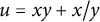. Then, for , we have $H^{\pm } (x, y) = O_{\kappa } ( \varPi T^{ \kappa } u )$ .

Proof This lemma follows from shifting the integral contour in (2.6) and (2.8) up to $\mathrm {Re} (it) = 1/2 + \varepsilon $ . For more details, see the proof of Lemma 4.1 in [Reference QiQi]. Note that for $\mathrm {Re}(\nu )> -1/2$ , we have the Poisson integral representation (see [Reference WatsonWat, Formula 3.71 (9)]):

$$ \begin{align*} I_{\nu } (x) = \frac { 2 ( x/2 )^{\nu }} {\sqrt{\pi} \Gamma (\nu + 1 / 2 ) } \int_0^{\frac 1 2 \pi} \cosh (x \cos \theta ) \sin^{2 \nu } \theta \, \mathrm{d} \theta.\\[-40pt] \end{align*} $$

For the rest of this section, let us assume that $ \unicode{x3b3} (t) $ lies in the space $ \mathscr {T}_{\tau }$ .

Lemma 4.2 Let $\unicode{x3b3} (t) $ be in the space $ \mathscr {T}_{\tau }$ . Let $A \geqslant 0$ . Then, for , we have

(4.7) $$ \begin{align} H^{\pm} (x, y) = \varPi T^{1+\tau} \int_{-\varPi^{\varepsilon }/\varPi}^{\varPi^{\varepsilon }/ \varPi} g ( \varPi r) \exp ( 2i T r) \cos ( f^{_{\phantom{i}}}_{^ \pm } (r; v, w) ) \mathrm{d} r + O \big(T^{-A}\big) , \end{align} $$

where

(4.8) $$ \begin{align} f^{_{\phantom{i}}}_{^ \pm } (r; v, w) = v \exp (r) \pm w \exp (- r) , \qquad v = \frac {xy} {2}, \quad w = \frac {x/y} 2, \end{align} $$

and $g (r)$ is a Schwartz function (namely, $ g^{(n)} (r) = O ( (|r|+1)^{-m})$ for any $m, n \geqslant 0$ ).

Later in our analysis, we shall always split

(4.9) $$ \begin{align} \cos ( f^{_{\phantom{i}}}_{^ \pm } (r; v, w) ) = \frac {\exp (i f^{_{\phantom{i}}}_{^ \pm } (r; v, w)) + \exp (- i f^{_{\phantom{i}}}_{^ \pm } (r; v, w) ) } {2}, \end{align} $$

so that we may extract the exponential factor $ \exp (\pm i v) $ or $\exp (\pm i w)$ , and we shall usually drop $g ( \varPi r) \exp ( 2i T r)$ as it does not involve $x, y$ or $v, w$ and is trivially $O (1)$ .

Proof This lemma follows essentially from inserting the Mehler–Sonine integrals (see [Reference WatsonWat, Formulas 6.21 (12) and 6.22 (13)])

$$ \begin{align*} {J_{2it} (x) - J_{-2it} (x)} & = \frac {2 \sinh ( \pi t) } {\pi i} \int_{-\infty}^{\infty} \cos (x \cosh r) \exp (2 i t r) \mathrm{d} r , \\ K_{2it} (x) & = \frac 1 {2 \cosh (\pi t)} \int_{-\infty}^{\infty} \cos (x \sinh r) \exp (2itr) \mathrm{d} r, \end{align*} $$

StartLayout 1st Row 1st Column upper J Subscript 2 i t Baseline left parenthesis x right parenthesis minus upper J Subscript minus 2 i t Baseline left parenthesis x right parenthesis 2nd Column equals StartFraction 2 hyperbolic sine left parenthesis pi t right parenthesis Over pi i EndFraction integral Subscript negative infinity Superscript infinity Baseline cosine left parenthesis x hyperbolic cosine r right parenthesis exp left parenthesis 2 i t r right parenthesis normal d r comma 2nd Row 1st Column upper K Subscript 2 i t Baseline left parenthesis x right parenthesis 2nd Column equals StartFraction 1 Over 2 hyperbolic cosine left parenthesis pi t right parenthesis EndFraction integral Subscript negative infinity Superscript infinity Baseline cosine left parenthesis x hyperbolic sine r right parenthesis exp left parenthesis 2 i t r right parenthesis normal d r comma EndLayout

into the Bessel integrals as in (2.6) and (2.7). For more details, see the proof of Lemma 4.3 in [Reference QiQi].

Moreover, Lemma 4.5 in [Reference QiQi] may be extended easily by applying stationary phase analysis to the integral in (4.7).

Lemma 4.3 Let $T^{\varepsilon } \leqslant \varPi \leqslant T^{1-\varepsilon }$ . Then, $H^{\pm } (x, y) = O (T^{-A} )$ if .

By Lemmas 4.1–4.3, we conclude that if $\unicode{x3b3} (t)$ is in $ \mathscr {Q}_{\tau } \cap \mathscr {T}_{\tau } $ , then the Bessel integrals $H^{\pm } (x, y)$ are negligibly small for .

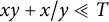Corollary 4.1 Let $\unicode{x3b3} (t)$ be in the space $ \mathscr {Q}_{\tau } \cap \mathscr {T}_{\tau } $ . Set $u = xy +x/y$ 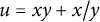as before. Then, for , we have

(4.10)

for any $A \geqslant 0$ .

Remark 4.1 Later, in practice, $ \unicode{x3b3} (t)$ will be those as defined in (6.8) and (6.9) for $|\mathrm {Im}(v)| \leqslant \log T$ or simply $\unicode{x3b3} (t) \equiv 1$ in Section 13. Note that Definition 4.1 requires $\unicode{x3b3} (t) $ to be holomorphic on the strip $ |\mathrm {Im} (t)| \leqslant 1/2 + \varepsilon $ . 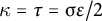For the odd case $\delta = 1$ , it follows from Lemma 6.4 that $ \unicode{x3b3} _{\sigma}^{1} (v, t) $ lies in $ \mathscr {Q}_{ \unicode{x3c3} \varepsilon /2} \cap \mathscr {T}_{ \unicode{x3c3} \varepsilon /2} $ 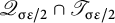if we let $\mathrm {Re} (v) = \varepsilon $ in (6.14), so we may just choose $\kappa = \tau = \unicode{x3c3} \varepsilon /2$ . For the even case $\delta = 0$ , however, it is slightly more subtle: In view of Lemma 6.4, we may apply Corollary 4.1 with $\mathrm {Re} (v) = 1$ and $ \tau = \unicode{x3c3} /2 $ say for , and use the integral representation (4.7) in Lemma 4.2 with $ \mathrm {Re} (v) = \varepsilon $ and $ \tau = \unicode{x3c3} \varepsilon /2$ for .

Remark 4.2 In [Reference QiQi, Section 4], we also studied the Bessel transform of a certain $h_{^ -}^{} (t; y)$ that contains the factor $\unicode{x3b5} ^{\delta } (t)$ defined similarly to (6.10), but here we shall not deal with this case (see the discussion at the end of Section 6.3).

Remark 4.3 In the study of related Maass central L-values, the $H^{+}$ and $H^{-}$ Bessel integrals have phases $x \cosh r$ and $x \sinh r$ , and hence behave quite differently in [Reference LiLi1] or [Reference YoungYou, Section 7]; but here, as we have just seen, the phases are $f^{_{\phantom {i}}}_{^ \pm } (r; v, w) = v \exp (r) \pm w \exp (- r)$ and may be analyzed more or less in the same way.

5 A useful unsmoothing lemma

As in (4.2), for large parameters $T, \varPi $ with $T^{\varepsilon } \leqslant \varPi \leqslant T^{1-\varepsilon }$ , define

(5.1) $$ \begin{align} \unicode{x3D5} (t) = \unicode{x3D5}_{T, \varPi} (t) = \exp \left( - \frac {(t-T)^2} {\varPi^2} \right)\!. \end{align} $$ StartLayout 1st Row normal phi left parenthesis t right parenthesis equals normal phi Subscript upper T comma upper Pi Baseline left parenthesis t right parenthesis equals exp left parenthesis minus StartFraction left parenthesis t minus upper T right parenthesis squared Over upper Pi squared EndFraction right parenthesis period EndLayout

In this section, we introduce a useful unsmoothing process as in [Reference Ivić and JutilaIJ, Section 3] by an average of the weight $\unicode{x3D5} _{T, \varPi } $ in the T-parameter.

Definition 5.1 Let $ H \leqslant T / 3 $ and $T^{\varepsilon } \leqslant \varPi \leqslant H^{1-\varepsilon } $ . Define

(5.2) $$ \begin{align} \unicode{x3c8} (t) = \unicode{x3C8}_{T, \varPi, H} (t) = \frac 1 { \sqrt{\pi} \varPi} \int_{\, T- H}^{T + H} \unicode{x3D5}_{K, \varPi} (t) \mathrm{d} K. \end{align} $$

The next lemma is essentially Lemma 5.3 in [Reference Liu and QiLQ2], adapted from the arguments in [Reference Ivić and JutilaIJ, Section 3].

Lemma 5.1 Let $\lambda $ be a real constant. Suppose that $a_f $ is a sequence such that

(5.3)

for any $\varPi $ with $ T^{\varepsilon } \leqslant \varPi \leqslant T^{1-\varepsilon } $ . Then, for $ \varPi ^{1+\varepsilon } \leqslant H \leqslant T / 3, $ we have

(5.4)

Later, we shall choose $a_f$ to be $\delta (L (s_f, f ) \neq 0)$ (the Kronecker $\delta $ that detects $L (s_f, f ) \neq 0$ ), $L (s_f, f ) $ , or $|L (s_f, f )|^2$ (see Sections 10.4, 11, and 16). Note that in all these cases, we may let $\lambda = 1$ or $ 1+\varepsilon $ in (5.3) in light of the (harmonic-weighted) Weyl law or the mean Lindelöf bounds.

Part I

Twisted and mollified moments

6 Preliminaries

6.1 Poisson summation formula

The following Poisson summation formula is essentially [Reference Iwaniec and KowalskiIK, Formula (4.25)].

Lemma 6.1 Let $\alpha , c $ be integers with $c \geqslant 1$ . Then, for $F (x) \in C_c^{\infty } (-\infty , \infty ),$ we have

(6.1) $$ \begin{align} \sum_{n } e \left ( \frac {\alpha n} c \right ) F (n) & = \sum_{n \equiv - \alpha (\mathrm{mod}\, c) } \hat {F} \Big( \frac {n} {c} \Big) , \end{align} $$

where $ \hat {F} (y)$ is the Fourier transform of $F (x)$ defined by

$$ \begin{align*} \hat {F} (y) = \int_{-\infty}^{\infty} F (x) e ( - x y) \mathrm{d} x. \end{align*} $$

6.2 Mean-value bounds for the Riemann $\zeta $ function

The best bound for the mean square of $ \zeta (1/2+it) $ on short intervals is due to Bourgain and Watt [Reference Bourgain and WattBW, Theorem 3]:

(6.2)

From this and the Cauchy–Schwarz inequality, we deduce easily the next lemma.

Lemma 6.2 Let $1 \leqslant H \leqslant T/3$ . We have

(6.3)

(6.4)

6.3 Approximate functional equations

Let $X> 1$ be a large parameter. By applying [Reference Iwaniec and KowalskiIK, Theorem 5.3] to $L ( s , f )$ at $s = s_f$ and to $ L (s+it_f , f ) L (s-it_f, f ) $ at $s = 1/2$ , we deduce, from (3.1) and (3.2), the approximate functional equations:

(6.5) $$ \begin{align} L ( s_f , f ) = \! \sum_{n=1}^{\infty} \! \frac{ \lambda_f (n) }{n^{1/2 + i t_f}} V_{1}^{\delta_f} ( n/X; t_f ) + (-1)^{\delta_f} \unicode{x3b5}^{\delta_f} (t_f) \! \sum_{n=1}^{\infty} \! \frac{ \lambda_f (n) }{n^{1/2 - i t_f}} V_{1}^{\delta_f} ( n X; - t_f ), \end{align} $$

(6.6) $$ \begin{align} \begin{aligned} |L ( s_f , f )|^2 = 2 \sum_{n_1=1}^{\infty} \sum_{n_2=1}^{\infty} \frac{ \lambda_f (n_1) \lambda_f (n_2) }{n_1^{1/2 + i t_f} n_2^{1/2 - i t_f}} V_{2}^{\delta_f} ( n_1 n_2; t_f ), \end{aligned} \end{align} $$

with

(6.7) $$ \begin{align} V_{\unicode{x3c3}}^{\delta} (y; t) = \frac 1 {2\pi i} \int_{(3)} \unicode{x3b3}_{\unicode{x3c3}}^{\delta} (v, t) y^{-v} \frac {\mathrm{d} v} {v} , \qquad \unicode{x3c3} = 1, 2, \end{align} $$

where

(6.8) $$ \begin{align} \unicode{x3b3}_{1}^{\delta} (v, t) = \exp (v^2) \frac {\Gamma_{\mathbf{R}}^{\delta} (1/2 + v ) \Gamma_{\mathbf{R}}^{\delta} (1/2 + v + 2 it) } {\Gamma_{\mathbf{R}}^{\delta} (1/2 ) \Gamma_{\mathbf{R}}^{\delta} (1/2 + 2 it) } , \end{align} $$

(6.9) $$ \begin{align} \unicode{x3b3}_{2}^{\delta} (v, t) = \exp (v^2) \frac {\Gamma_{\mathbf{R}}^{\delta} (1/2 + v )^2 \Gamma_{\mathbf{R}}^{\delta} (1/2 + v + 2 it) \Gamma_{\mathbf{R}}^{\delta} (1/2 + v - 2 it) } { \Gamma_{\mathbf{R}}^{\delta} (1/2 )^2 \Gamma_{\mathbf{R}}^{\delta} (1/2 + 2 it) \Gamma_{\mathbf{R}}^{\delta} (1/2 - 2 it) } , \end{align} $$

(6.10) $$ \begin{align} \unicode{x3b5}^{\delta} (t) = \frac {\Gamma_{\mathbf{R}}^{\delta} (1/2 - 2 it)} {\Gamma_{\mathbf{R}}^{\delta} (1/2 + 2 it)}. \end{align} $$ epsilon Superscript delta Baseline left parenthesis t right parenthesis equals StartFraction normal upper Gamma Subscript bold upper R Superscript delta Baseline left parenthesis 1 divided by 2 minus 2 i t right parenthesis Over normal upper Gamma Subscript bold upper R Superscript delta Baseline left parenthesis 1 divided by 2 plus 2 i t right parenthesis EndFraction period

Moreover, in parallel, we have

(6.11) $$ \begin{align} \zeta (1/2) \zeta (1/2+2it) = \sum_{n=1}^{\infty} \frac{ \tau_{ it} (n) }{n^{1/2 + i t}} V_{1}^{0} ( n/X; t ) + \unicode{x3b5}^{0} (t) \sum_{n=1}^{\infty} \frac{ \tau_{ it} (n) }{n^{1/2 - i t}} V_{1}^{0} ( n X; - t ), \end{align} $$

(6.12) $$ \begin{align} |\zeta (1/2) \zeta (1/2+2it) |^2 = 2 \sum_{n_1=1}^{\infty} \sum_{n_2=1}^{\infty} \frac{ \tau_{ it} (n_1) \tau_{ it} (n_2) }{n_1^{1/2 + i t} n_2^{1/2 - i t}} V_{2}^{0} ( n_1 n_2; t ), \end{align} $$

up to certain residual error terms of bounds $ O \big ( (|t| + 1)^{1/4+\varepsilon } X^{1/2} \big ) $ and $O \big (\exp (- t^2/2) \big ) $ 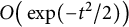, respectively.

The next two lemmas are standard consequences of the Stirling formula. Compare [Reference Iwaniec and KowalskiIK, Proposition 5.4], [Reference BlomerBlo, Lemma 1], and [Reference QiQi, Lemmas 3.6 and 3.7].

Lemma 6.3 Let and $\theta> 0$ . Then, for $\unicode{x3c3} = 1, 2$ , we have

(6.13)

for any $A \geqslant 0$ , and

(6.14) $$ \begin{align} {V}_{\unicode{x3c3}}^{\delta} (y; t) = \frac 1 {2\pi i} \int_{\theta - i U}^{\theta +i U} \unicode{x3b3}_{\unicode{x3c3}}^{\delta} (v, t) y^{-v} \frac {\mathrm{d} v} {v} + O_{\theta } \bigg( \frac {(|t|+1)^{\unicode{x3c3} \theta /2 } } {y^{\theta} \exp (U^2/2)} \bigg). \end{align} $$

Lemma 6.4 Let $\mathrm {Re}(v)> - 1/2$ be fixed. Then, for $|\mathrm {Re} (it)| < \mathrm {Re}(v/2) + 1/4 + \delta /2 $ , we have

(6.15)

and, for t real, we have

(6.16)

for any $n \geqslant 0$ .

The reader should compare Lemma 6.4 with Definitions 4.1 and 4.2.

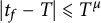
Later, the analysis will be restricted to the range $|t_f-T|, \, |t - T| \leqslant \varPi \log T$ , so it follows from (6.13) that the second sum in (6.5) or (6.11) (after $\unicode{x3b5} ^{\delta _f} (t_f)$ or $\unicode{x3b5} ^{0} (t) $ ) will be negligibly small if we choose

$$ \begin{align*}X = T^{1/2+\varepsilon },\end{align*} $$

while the first sum may be truncated effectively at $ n = T^{1+\varepsilon } $ . Moreover, the residual error term for (6.11) has bound $O (T^{1/2+\varepsilon })$ . Note that the error term in (6.14) is negligibly small if we choose

$$ \begin{align*}U = \log T.\end{align*} $$

6.4 Bi-variable notation

Subsequently, particularly in our study of the second twisted moment in Section 9, we shall use bold $\boldsymbol {m}$ , $\boldsymbol {n}$ , $\ldots $ for the (positive integral) pairs $(m_1, m_2)$ , $(n_1, n_2)$ , $\ldots $ . Define the norm $ \|\boldsymbol {n}\| = n_1 n_2 $ , the fraction $\langle \boldsymbol {n} \rangle = n_1/ n_2$ , the dual $\widetilde {\boldsymbol {n}} = (n_2, n_1)$ , the reduction $\boldsymbol {n}^{\star } = \boldsymbol {n} / \mathrm {gcd}(\boldsymbol {n}) $ , the product $ \boldsymbol {m n} = (m_1 n_1, m_2 n_2) $ , and the quotient $ {\boldsymbol {m}/ \boldsymbol {n} = (m_1 / n_1, m_2 / n_2)} $ . Let $\delta (\boldsymbol {n})$ be the Kronecker $\delta $ that detects $n_1 = n_2$ .

Define

(6.17) $$ \begin{align} \mathrm{c}_t ( \boldsymbol{n}) = \mathrm{Re} \big((n_1/n_2)^{it} \big) = \cos (t \log (n_1/n_2)). \end{align} $$

For an arithmetic function $a (n)$ , define

(6.18) $$ \begin{align} a (\boldsymbol{n}) = a (n_1) a (n_2). \end{align} $$

For instance, (1.9) now reads

(6.19)

Occasionally, we shall use $\boldsymbol {x} $ for the positive real pair $(x_1 , x_2)$ , and, similar to (6.18), for a smooth function $\textit {w} (x)$ write

(6.20) $$ \begin{align} \textit{w} (\boldsymbol{x}) = \textit{w} ( {x}_1 ) \textit{w} ({x}_2). \end{align} $$

7 Setup

For large parameters $T, \varPi $ with $T^{\varepsilon } \leqslant \varPi \leqslant T^{1-\varepsilon }$ , let us define

(7.1) $$ \begin{align} \unicode{x3D5} (t) = \exp \left( - \frac {(t-T)^2} {\varPi^2} \right)\!, \end{align} $$ normal phi left parenthesis t right parenthesis equals exp left parenthesis minus StartFraction left parenthesis t minus upper T right parenthesis squared Over upper Pi squared EndFraction right parenthesis comma

and consider

(7.2)

(7.3)

Note that or respectively, differs from or as in (1.8) or (1.9) (see also (6.19)) merely by an exponentially small error term. In parallel, the Eisenstein contributions read

(7.4)

(7.5)

where we have used the t-evenness of $\omega (t)$ , $ \tau _{it} (m) $ , and $ \mathrm {c}_{ t } (\boldsymbol {m}) $ .

Lemma 7.1 We have

(7.6)

(7.7)

Proof Since $ \omega (t) = O ( |t|^{\varepsilon } )$ by [Reference TitchmarshTit, Formula (3.11.10)], it is clear that (7.6) and (7.7) follow from (6.3) and (6.4) in Lemma 6.2, respectively, if we choose $H = \varPi \log T$ .

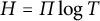
8 The twisted first moment

8.1 Application of the Kuznetsov formula

By the approximate functional equations (6.5) and (6.11), with

$$ \begin{align*}X = T^{1/2+\varepsilon },\end{align*} $$

we have

C sub 1 natural super delta (m) equals summation n=1 to infinity 1 all over square root n summation f in B sub delta omega sub f lambda sub f (m) lambda sub f (n) V sub 1 super delta (m, n; t sub f) + O(T^-A). E sub 1 (m) equals summation n=1 to infinity 1 all over square root n times 1 all over pi integral -infinity to infinity omega(t) tau sub it (m) tau sub it (n) V sub 1 super 0 (m, n; t) dt + O(Pi T^1/2+epsilon).

where the error terms are due to the discussions at the end of Section 6.3, and

(8.1) $$ \begin{align} {V}_{1}^{\delta} (m, n; t) = V_{1}^{\delta} ( n/ X; t ) (m n)^{ - i t} {\unicode{x3D5} (t)} + V_{1}^{\delta} ( n/X; - t ) (mn)^{ i t} {\unicode{x3D5} (- t)}. \end{align} $$

It follows from the Kuznetsov trace formula in (2.9) that

(8.2)

with the diagonal

(8.3)

where

(8.4) $$ \begin{align} H_1^{\delta} (m ) = \frac 1 {\pi^2 } \int_{-\infty}^{\infty} {V}_{1}^{\delta} (m, m; t) \tanh(\pi t) t \mathrm{d} t , \end{align} $$

and the off-diagonal

(8.5)

where

(8.6) $$ \begin{align} {H}_1^{\delta\, +} (x; m, n) & = \frac {2i} {\pi} \int_{-\infty}^{\infty} {V}_{1}^{\delta} (m, n; t) J_{2it} (x) \frac {t \mathrm{d} t} {\cosh (\pi t) } , \end{align} $$

(8.7) $$ \begin{align} {H}_1^{\delta\, -} (x; m, n) & = \frac {4} {\pi^2} \int_{-\infty}^{\infty} {V}_{1}^{\delta} (m, n; t) K_{2it} ( x) {\sinh (\pi t)} t \, \mathrm{d} t. \end{align} $$

8.2 Asymptotic for the diagonal term

In view of (8.1) and (8.4), we have

$$ \begin{align*} {H}_{1}^{\delta} (m ) = \frac {2} {\pi^2} \int_{-\infty}^{\infty} V_{1}^{\delta} ( m/ X; t ) m^{ - 2 i t} {\unicode{x3D5} (t)} \tanh(\pi t) t \mathrm{d} t. \end{align*} $$

Keep in mind that $\unicode{x3D5} (t)$ as in (7.1) is negligibly small unless $|t - T | \leqslant \varPi \log T$ . Thus, up to an exponentially small error, $\tanh (\pi t) $ is removable as $\tanh (\pi t) = 1 + O (\exp (-\pi T))$ on this range.

Let us first evaluate . By shifting the integral contour in (6.7) from $\mathrm {Re} (v) = 3$ down to $\mathrm {Re} (v) = \varepsilon -1/2 $ , we have

$$ \begin{align*} V_{1}^{\delta} (1/X; t) = 1 + O \bigg( \frac 1 { { (X \sqrt{|t|+1} )^{1/2 - \varepsilon }} } \bigg), \end{align*} $$ upper V 1 Superscript delta Baseline left parenthesis 1 divided by upper X semicolon t right parenthesis equals 1 plus upper O left parenthesis StartFraction 1 Over left parenthesis upper X StartRoot StartAbsoluteValue t EndAbsoluteValue plus 1 EndRoot right parenthesis Superscript 1 divided by 2 minus epsilon Baseline EndFraction right parenthesis comma

by the Stirling formula. Therefore,

$$ \begin{align*} {H}_{1}^{\delta} (1) = \frac {2} {\pi^2} \int_{-\infty}^{\infty} {\unicode{x3D5} (t)} t \mathrm{d} t + O (\varPi T^{1/2 +\varepsilon } ) , \end{align*} $$

as $X = T^{1/2+\varepsilon }$ , whereas

$$ \begin{align*} \int_{-\infty}^{\infty} {\unicode{x3D5} (t)} t \mathrm{d} t = \varPi T \int_{-\infty}^{\infty} \exp (-t^2) \mathrm{d} t = { \sqrt{\pi}} \varPi T. \end{align*} $$

Consequently,

Note that in the odd case of the error term may be improved into $O (\varPi / T^{1/2-\varepsilon })$ 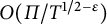by shifting the integral contour further down to $\mathrm {Re} (v) = \varepsilon -3/2 $ .

Next, we consider the case $m> 1$ . By inserting the integral in (6.14), with $\theta = \varepsilon $ and $U = \log T$ , we arrive at

$$ \begin{align*} {H}_{1}^{\delta} (m ) = \frac {1} {\pi^3 i} \int_{\varepsilon -i\log T}^{\varepsilon +i\log T} \int_{T-\varPi \log T}^{T+\varPi \log T} \frac { \unicode{x3b3}_{1}^{\delta} (v, t) {\unicode{x3D5} (t)} t } { m^{v+2it} / X^{v} } \frac { \mathrm{d} t \mathrm{d} v} { v} + O \big(T^{-A} \big). \end{align*} $$

For $t $ and $ v$ on the integral domains, in view of (6.8), it follows from the Stirling formula that

$$ \begin{align*} \unicode{x3b3}_{1}^{\delta} (v, t) = \unicode{x3b3}_{1}^{\delta} (v) \big( t^{v/2} + O ( {T^{\varepsilon } } / T ) \big) , \quad \unicode{x3b3}_{1}^{\delta} (v) = \exp \Big(v^2 + \frac {v} 2 \log ( i/\pi ) \Big) \frac {\Gamma_{\mathbf{R}}^{\delta} (1/2 + v ) } {\Gamma_{\mathbf{R}}^{\delta} (1/2 )}. \end{align*} $$

Therefore,

$$ \begin{align*} H_{1}^{\delta} (m) = \frac {1} {\pi^3 i} \int_{\varepsilon -i\log T}^{\varepsilon +i\log T} \frac {\unicode{x3b3}_{1}^{\delta} (v)} {(m/X)^{v} } \int_{T-\varPi \log T}^{T+\varPi \log T} { {\unicode{x3D5} (t)} t^{1+v/2} } m^{-2it} \mathrm{d} t \, \frac { \mathrm{d} v} { v} + O ( {\varPi T^{\varepsilon }} ). \end{align*} $$

For $m> 1$ , the inner t-integral is Fourier of phase $ - 2 t \log m$ ; so, by repeated partial integration, we infer that the integral is negligibly small. Consequently, we have $ H_1^{\delta } (m) = O (\varPi T^{\varepsilon }) $ , and hence

To summarize, we conclude with the following lemma for .

Lemma 8.1 We have

(8.8)

8.3 Estimation of the off-diagonal sums

Let us consider the off-diagonal sums given by (8.1) and (8.5)–(8.7).

By (6.13) in Lemma 6.3 (see also the discussion at the end of Section 6.3) along with a smooth dyadic partition, at the cost of a negligible error, we may confine the n-sum in (8.5) on the range $ n \sim N $ for dyadic (namely, N is of the form $2^{j/2}$ ). Next, we insert the expression of $ V_{1}^{\delta } ( n / X; t ) $ as in (6.14) in Lemma 6.3 into (8.1), (8.6), and (8.7). After this, there arise the Bessel transforms $H_1^{\delta \, \pm } (x, y; v)$ 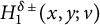of the function

$$ \begin{align*} h_{1}^{\delta} (t; y; v) = \unicode{x3b3}_{1}^{\delta} (v, t) y^{-2it} \unicode{x3D5} (t) + \unicode{x3b3}_{1}^{\delta} (v, - t) y^{2it} \unicode{x3D5} (- t), \end{align*} $$

as in Section 4, for

$$ \begin{align*} x = \frac {4\pi \sqrt{mn}} {c}, \qquad y = \sqrt{m n}. \end{align*} $$

Since $\delta $ and v are not essential in our analysis, they will usually be omitted in the sequel. By Corollary 4.1 and Remark 4.1, along with the Weil bound (2.11), we may further restrict the c-sum in (8.5) to the range . It follows that up to a negligible error, the off-diagonal sum has bound

(8.9)

where, if we omit $\delta $ and v from the notation,

(8.10)

with

$$ \begin{align*} \textit{w} (x) = \frac {\textit{v} (x)} {x^{1/2+v}}, \end{align*} $$

for a certain fixed smooth weight $\textit {v} \in C_c^{\infty }[1,2]$ . Note that v will not play a role since we have uniformly

Next, in (8.10), we open the Kloosterman sum $S (m, \pm n;c)$ (see (2.10)) and insert the formula of the Bessel integrals $H_1^{ \pm } (x, y)$ as in Lemma 4.2. For the latter, we have

$$ \begin{align*} v = \frac {2\pi m n} {c}, \qquad w = \frac {2\pi} {c}; \end{align*} $$

then, we split $\cos ( f^{_{\phantom {i}}}_{^{\pm } } (r; v, w) )$ as in (4.9) and extract the exponential factor $e (mn/ c)$ or $ e (- mn/ c) $ . It follows that

(8.11)

where

(8.12)

with

$$ \begin{align*}\unicode{x3c1} (r) = \exp (r) - 1,\end{align*} $$

$\textit {w}^{_{\phantom {i}}}_{^ +} (x) = \textit {w} (x) $ , and $\textit {w}^{_{\phantom {i}}}_{^ -} (x) = \overline {\textit {w} (x) }$ 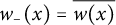. On applying to the n-sum the Poisson summation formula in Lemma 6.1, we have

O plus or minus (r; m, c; N) = N summation over alpha mod c of e (plus or minus alpha-bar m all over c) summation over n congruent to minus alpha minus m mod c of w-hat plus or minus (N(n minus m rho(r)) all over c).

Note that the Fourier transform $ \hat {\textit {w}}^{_{\phantom {i}}}_{^ \pm } ( N (n-m \unicode{x3c1} (r))/ c ) $ is negligibly small unless

(8.13) $$ \begin{align} | n-m \unicode{x3c1} (r) | < \frac {c T^{\varepsilon }} {N}. \end{align} $$

we may restrict the n-sum to the range . Consequently, up to a negligible error,

Now the r-integral may be confined further to the interval defined by (8.13) of length $ O (cT^{\varepsilon } / m N) $ 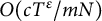, and hence

(8.14)

On inserting (8.14) into (8.11), we have

(8.15)

Note that the implicit constant in (8.15) depends on $\varepsilon $ but is uniform for all $ v \in [\varepsilon - i \log T, \varepsilon + i \log T]$ . Consequently, from (8.9) and (8.15), we deduce the following bound for .

Lemma 8.2 We have

(8.16)

8.4 Conclusion

In view of (8.2), Theorem 5 is a direct consequence of Lemmas 7.1, 8.1, and 8.2.

9 The twisted second moment

As the bi-variable notation will be used frequently in what follows, the reader is advised to read Section 6.4 before proceeding with this section.

9.1 Application of the Kuznetsov formula

First, in the bi-variable notation, by the approximate functional equations (6.6) and (6.12) (here, we need to expand $2 \mathrm {c}_t ( \boldsymbol {m} ) \mathrm {c}_t ( \boldsymbol {n}) = \mathrm {c}_t ( \boldsymbol {m} \boldsymbol {n}) + \mathrm {c}_t ( \boldsymbol {m} / \boldsymbol {n}) $ (see (6.17)) and use the symmetry in the $\boldsymbol {n}$ -sums), we obtain

C sub 2 natural super delta (m) equals summation over n of 1 all over square root of norm n times summation over f in B sub delta of omega sub f lambda sub f (m) lambda sub f (n) V sub 2 super delta (m, n; t sub f). E sub 2 (m) equals summation over n of 1 all over square root of norm n times 1 all over pi integral from minus infinity to infinity of omega (t) tau sub i t (m) tau sub i t (n) V sub 2 super 0 (m, n; t) d t plus O (T super minus A).

where $ \boldsymbol {n} = (n_1, n_2)$ and $ \| \boldsymbol {n}\| = n_1 n_2 $ as in Section 6.4, and

$$ \begin{align*} {V}_{2}^{\delta} (\boldsymbol{m}, \boldsymbol{n}; t) = 2 V_2^{\delta} ( \| \boldsymbol{n} \|; t) \mathrm{c}_t ( \boldsymbol{m} \boldsymbol{n}) ( \unicode{x3D5} (t) + \unicode{x3D5} (- t) ). \end{align*} $$

Note that $ {V}_{2}^{\delta } (\boldsymbol {m}, \boldsymbol {n}; t)$ is even in t and real-valued. By the Hecke relation (2.12),

C sub 2 natural super delta (m) equals summation over d h equals m summation over n of 1 all over square root of norm d n summation over f in B sub delta of omega sub f lambda sub f (h n) V sub 2 super delta (m, d n; t sub f).

where, according to the bi-variable notation in Section 6.4, the first summations are over $ \boldsymbol {d} = (d_1, d_2) $ and $ \boldsymbol {h} = (h_1, h_2)$ such that $ (d_1 h_1, d_2 h_2) = (m_1, m_2)$ . Now an application of the Kuznetsov trace formula in (2.9) yields

(9.1)

with the diagonal

(9.2)

where $ \delta (\boldsymbol {hn}) $ is the Kronecker $\delta $ that detects $ h_1 n_1 = h_2 n_2 $ , and since $ \mathrm {c}_{t} ( \boldsymbol {d^2 h n} ) = \mathrm {c}_{2t} ( \boldsymbol {d} ) $ if $\delta (\boldsymbol {hn}) = 1$ ,

(9.3) $$ \begin{align} {H}_2^{\delta } (\boldsymbol{d}, \boldsymbol{ n} ) = \frac 4 {\pi^2 } \int_{-\infty}^{\infty} V_2^{\delta } ( \| \boldsymbol{n} \|; t) \mathrm{c}_{2t} ( \boldsymbol{d} ) \unicode{x3D5} (t) \tanh(\pi t) t \mathrm{d} t , \end{align} $$

and the off-diagonal

(9.4)

where $\boldsymbol {1}_{\pm } = (1, \pm 1)$ ; hence, $S ( \boldsymbol {1}_{\pm } \boldsymbol {h n}; c) = S (h_1 n_1, \pm h_2 n_2; c)$ , and

(9.5) $$ \begin{align} {H}_2^{\delta\, +} ( x; \boldsymbol{m}, \boldsymbol{n} ) & = \frac {4 i} {\pi} \int_{-\infty}^{\infty} {V}_2^{\delta} ( \| \boldsymbol{n} \|; t) \mathrm{c}_t ( \boldsymbol{m n}) ( \unicode{x3D5} (t) + \unicode{x3D5} (- t) ) J_{2it} (x) \frac {t \mathrm{d} t} {\cosh (\pi t) }, \end{align} $$

(9.6) $$ \begin{align} {H}_2^{\delta\, -} ( x; \boldsymbol{m}, \boldsymbol{n} ) & = \frac {8} {\pi^2} \!\int_{-\infty}^{\infty}\!\! {V}_2^{\delta} ( \| \boldsymbol{n} \|; t) \mathrm{c}_t ( \boldsymbol{m n}) ( \unicode{x3D5} (t) + \unicode{x3D5} (- t) ) K_{2it} ( x) {\sinh (\pi t)} t \mathrm{d} t. \end{align} $$

9.2 Asymptotic for the diagonal sum

Set

$$ \begin{align*} h = \mathrm{gcd}(\boldsymbol{h}), \qquad \boldsymbol{h^{\star}} = \boldsymbol{h} / h; \end{align*} $$

then, $ \delta ({\boldsymbol {h n} }) = 1 $ if and only if there is n such that $ \boldsymbol {n} = n \widetilde {\boldsymbol {h^{\star } }}. $ Recall from Section 6.4 that $ \widetilde {\boldsymbol {h^{\star }}} $ is dual to $\boldsymbol {h^{\star }}$ . Therefore, (9.2) is turned into

(9.7)

In view of (6.13) and (9.3), the summation in (9.7) may be restricted effectively to $ n \sqrt {\| \boldsymbol {m} \|} / h \leqslant T^{1/2+\varepsilon }$ . It follows from (6.13) and (7.1) that $ H_2^{\delta } (\boldsymbol {d}, \boldsymbol {n}) = O (\varPi T) $ ; so trivial estimation yields

where $\boldsymbol {m^{\star }} = \boldsymbol {m} / \mathrm {gcd} (\boldsymbol {m})$ . However, our aim here is to derive an asymptotic formula for .

Lemma 9.1 We have

(9.8) $$ \begin{align} {H}_2^{\delta} (\boldsymbol{d}, \boldsymbol{ n} ) = O \bigg( \frac {\varPi T^{\varepsilon }} { \| \boldsymbol{n} \|^{\varepsilon }} \bigg), \end{align} $$ upper H 2 Superscript delta Baseline left parenthesis bold italic d comma bold italic n right parenthesis equals upper O left parenthesis StartFraction upper Pi upper T Superscript epsilon Baseline Over StartMetric bold italic n EndMetric Superscript epsilon Baseline EndFraction right parenthesis comma

(9.9) $$ \begin{align} | \langle \boldsymbol{d} \rangle - 1 |> \frac {\varPi^{\varepsilon }} {\varPi}, \qquad ( \langle \boldsymbol{d} \rangle = d_1/d_2). \end{align} $$

Proof By (6.14), with $\theta = \varepsilon $ and $U = \log T$ , we have

$$ \begin{align*} {H}_2^{\delta} (\boldsymbol{d}, \boldsymbol{ n} ) = \frac {2} {\pi^3 i} \int_{\varepsilon -i\log T}^{\varepsilon +i\log T} \int_{T-\varPi \log T}^{T+\varPi \log T} \frac { \unicode{x3b3}_{2}^{\delta} (v, t) \mathrm{c}_{2t} ( \boldsymbol{d} ) {\unicode{x3D5} (t)} t } { \| \boldsymbol{n} \|^v } \frac { \mathrm{d} t \mathrm{d} v} { v} + O \big(T^{-A} \big). \end{align*} $$

For t and v on the integral domains, in view of (6.9), we have by the Stirling formula that

$$ \begin{align*} \unicode{x3b3}_{2}^{\delta} (v, t) = \unicode{x3b3}_{2}^{\delta} (v) \big( t^{ v} + O ( {T^{\varepsilon } } / T ) \big) , \qquad \unicode{x3b3}_{2}^{\delta} (v) = \exp (v^2 ) \pi^{-v} \frac {\Gamma_{\mathbf{R}}^{\delta} (1/2 + v )^2 } {\Gamma_{\mathbf{R}}^{\delta} (1/2 )^2 }. \end{align*} $$

Consequently,

$$ \begin{align*} {H}_2^{\delta} (\boldsymbol{d}, \boldsymbol{ n} ) = \frac {2} {\pi^3 i} \int_{\varepsilon -i\log T}^{\varepsilon +i\log T} \frac { \unicode{x3b3}_{2}^{\delta} (v) } { \| \boldsymbol{n} \|^v } \int_{T-\varPi \log T}^{T+\varPi \log T} { \mathrm{c}_{2t} ( \boldsymbol{d} ) {\unicode{x3D5} (t)} t^{1+ v} } \mathrm{d} t \frac { \mathrm{d} v} { v} + O \bigg(\frac {\varPi T^{\varepsilon }} { \| \boldsymbol{n} \|^{\varepsilon }} \bigg). \end{align*} $$

The inner t-integral is a cosine Fourier integral of phase $ 2 t \log \, \langle \boldsymbol {d} \rangle $ (see (6.17)); so, by repeated partial integration, we infer that it is negligibly small since by (9.9).

By Lemma 9.1, the off-diagonal terms with $ \delta (\boldsymbol {d}) = 0 $ contribute $ O (\varPi T^{\varepsilon } / \sqrt {\|\boldsymbol {m^{\star }}\| }) $ since our assumption $ \max \{ \boldsymbol {m} \} < \varPi ^{1-\varepsilon }$ yields $ |\langle \boldsymbol {d} \rangle - 1|> \varPi ^{\varepsilon }/ \varPi $ .

It is left to consider those diagonal terms with $ \delta (\boldsymbol {d}) = 1 $ . Note that, in this case, $ \boldsymbol {h^{\star }} = \boldsymbol {m^{\star }} $ . More explicitly, (9.7) is turned into

(9.10)

where, after the removal of $\tanh (\pi t)$ ,

(9.11) $$ \begin{align} H_2^{\delta} ( x ) = \frac 4 {\pi^2 } \int_{-\infty}^{\infty} V_2^{\delta} ( x^2; t) \unicode{x3D5} (t) t \mathrm{d} t. \end{align} $$

As, in (1.11), we set

$$ \begin{align*} m = \mathrm{gcd}(\boldsymbol{m}), \qquad r = \| \boldsymbol{m^{\star} } \|. \end{align*} $$

It follows from (6.7), (9.10), and (9.11) that

(9.12)

Now we shift the integral contour from $\mathrm {Re}(v) = 3$ down to $\mathrm {Re} (v) = \varepsilon -1/2$ and collect the residue at the double pole $v = 0$ . In view of (6.9) and (6.15), the resulting integral has bound $O ((|t|+1)^{\varepsilon -1/2} )$ and it yields the error $O (\varPi T^{1/2+\varepsilon })$ , while we have Laurent expansions (at $v = 0$ ):

$$ \begin{align*} \unicode{x3b3}_2^{\delta} (v, t) = 1 + (\unicode{x3c3}_2^{\delta} (t) - 4\log \pi) \frac {v} 2 + \cdots, \qquad \zeta (1+2v) = \frac 1 {2 v} + \gamma + \cdots , \end{align*} $$

$$ \begin{align*} \unicode{x3c3}_2^{\delta} (t) = 2 \psi ( \kappa ) + \psi ( \kappa + it ) + \psi ( \kappa - it ) , \qquad \kappa = \frac {1+2 \delta} 4 , \end{align*} $$

where $\gamma $ is the Euler constant and $\psi (s) = \Gamma '(s)/\Gamma (s)$ is the di-gamma function, and it follows that the residue is equal to

$$ \begin{align*} \frac 1 {d \sqrt{r}}\bigg( \gamma + \frac 1 4 \unicode{x3c3}_2^{\delta} (t) - \log (\pi d \sqrt{r}) \bigg). \end{align*} $$ StartFraction 1 Over d StartRoot r EndRoot EndFraction left parenthesis gamma plus one fourth normal sigma 2 Superscript delta Baseline left parenthesis t right parenthesis minus log left parenthesis pi d StartRoot r EndRoot right parenthesis right parenthesis period

By the Stirling formula,

$$ \begin{align*} \unicode{x3c3}_2^{\delta} (t) = 2 \psi ( \kappa ) + 2 \log \sqrt{ \kappa ^2 + t^2 } + O \bigg(\frac 1 {1+t^2} \bigg). \end{align*} $$ normal sigma 2 Superscript delta Baseline left parenthesis t right parenthesis equals 2 psi left parenthesis kappa right parenthesis plus 2 log StartRoot kappa squared plus t squared EndRoot plus upper O left parenthesis StartFraction 1 Over 1 plus t squared EndFraction right parenthesis period

Next, the t-integrals may be evaluated easily by

$$ \begin{align*} \int_{-\infty}^{\infty} {\unicode{x3D5} (t)} t \mathrm{d} t = { \sqrt{\pi}} \varPi T , \qquad \int_{-\infty}^{\infty} {\unicode{x3D5} (t)} t \log \sqrt{\kappa ^2+ t^2} \mathrm{d} t = { \sqrt{\pi}} \varPi T \log T + O \bigg(\frac {\varPi^3} T \bigg). \end{align*} $$

It is clear that the error after this process is $O (\varPi ^3T^{\varepsilon }/ T {\displaystyle \sqrt {r }})$ , while the main term reads

$$ \begin{align*} \frac {4} {\pi\sqrt{\pi r}} \varPi T \sum_{d |m} \frac 1 {d} \bigg( \gamma + \frac 1 2 \psi (\kappa ) + \log \frac {\sqrt{T}} {\pi d \sqrt{r}}\bigg). \end{align*} $$ StartFraction 4 Over pi StartRoot pi r EndRoot EndFraction upper Pi upper T sigma summation Underscript d vertical bar m Endscripts StartFraction 1 Over d EndFraction left parenthesis gamma plus one half psi left parenthesis kappa right parenthesis plus log StartFraction StartRoot upper T EndRoot Over pi d StartRoot r EndRoot EndFraction right parenthesis period

Moreover, by the Gauss di-gamma formula in [Reference Magnus, Oberhettinger and SoniMOS, Section 1.2],

$$ \begin{align*} \psi \bigg(\frac 1 4 \bigg) = - \gamma - 3\log 2 - \frac {\pi} 2, \qquad \psi \bigg(\frac 3 4 \bigg) = - \gamma - 3\log 2 + \frac {\pi} 2. \end{align*} $$ StartLayout 1st Row psi left parenthesis one fourth right parenthesis equals negative gamma minus 3 log 2 minus StartFraction pi Over 2 EndFraction comma psi left parenthesis three fourths right parenthesis equals negative gamma minus 3 log 2 plus StartFraction pi Over 2 EndFraction period EndLayout

Finally, we conclude with the following asymptotic formula for .

Lemma 9.2 Set

(9.13) $$ \begin{align} m = (m_1, m_2), \qquad r = \frac {m_1m_2} {m^2}. \end{align} $$

Define

(9.14) $$ \begin{align} \gamma_{0 } = \gamma - \log 8 \pi^2 - \frac {\pi} 2 , \qquad \gamma_1 = \gamma - \log 8 \pi^2 + \frac {\pi} 2, \end{align} $$

(9.15) $$ \begin{align} \sigma_{-1} ( m ) = {\sum_{d | m } } \frac {1} {d }, \qquad \sigma_{-1}' ( m ) = {\sum_{d | m } } \frac {\log d } {d }. \end{align} $$ StartLayout 1st Row sigma Subscript negative 1 Baseline left parenthesis m right parenthesis equals sigma summation Underscript d vertical bar m Endscripts StartFraction 1 Over d EndFraction comma sigma prime Subscript negative 1 Baseline left parenthesis m right parenthesis equals sigma summation Underscript d vertical bar m Endscripts StartFraction log d Over d EndFraction period EndLayout

Then,

(9.16)

D sub 2 super delta (m) = 2 all over pi square root of pi r times capital Pi T ( (log T over r + gamma sub delta) sigma sub -1 (m) - 2 sigma prime sub -1 (m) + O (T super epsilon (capital Pi square root of T + T over square root of r + capital Pi cubed over T square root of r) ) ).

9.3 Estimation of the off-diagonal sums

Similar to the initial arguments for in Section 8.3, by applying Lemma 6.3, Corollary 4.1, and Remark 4.1 to (9.4)–(9.6), we have

(9.17)

where $\boldsymbol {N} $ are dyadic, and

(9.18)

in which

(9.19) $$ \begin{align} C = \frac { \max \{ \boldsymbol{ m N } \} } {T \|\boldsymbol{d}\| } , \end{align} $$ upper C equals StartFraction max left brace bold italic m bold italic upper N right brace Over upper T StartMetric bold italic d EndMetric EndFraction comma

the weight $\textit {w} (\boldsymbol {x})$ is of the product form as in (6.20) for the weight function $\textit {w} \in C_c^{\infty } [1, 2]$ 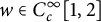as in Section 8.3, and $H_{2}^{ \pm } (x, y ) $ are the Bessel transforms of

$$ \begin{align*} h_{2} (t; y ) = 2 \unicode{x3b3}_{2}^{\delta} (v, t) \cos (2t \log y) (\unicode{x3D5} (t) + \unicode{x3D5} (- t)), \end{align*} $$

as in (4.3); here $\delta $ and v have been suppressed again from the notation.

By the formula of the Bessel integrals $H^{ \pm } (x, y ) $ as in Lemma 4.2, along with (4.4) and (4.9), it follows that splits into four similar parts, one of which is

(9.20)

with

(9.21)

where

(9.22) $$ \begin{align} T_{\pm} ( \boldsymbol{ n}; \boldsymbol{d}; c) = S(n_1, \pm n_2; c ) e \bigg(\frac {d_1 n_1} {c d_2 } \pm \frac {d_2 n_2} {c d_1 } \bigg), \end{align} $$ upper T Subscript plus or minus Baseline left parenthesis bold italic n semicolon bold italic d semicolon c right parenthesis equals upper S left parenthesis n 1 comma plus or minus n 2 semicolon c right parenthesis e left parenthesis StartFraction d 1 n 1 Over c d 2 EndFraction plus or minus StartFraction d 2 n 2 Over c d 1 EndFraction right parenthesis comma

(9.23) $$ \begin{align} \unicode{x3c1}^{_{\phantom{i}}}_{^ \pm} (r; \boldsymbol{ n} , \boldsymbol{d}; c) = \frac {d_1 n_1} {c d_2} \unicode{x3b3}_1 (r) \pm \frac {d_2 n_2} {c d_1} \unicode{x3b3}_2 (r), \end{align} $$

for

$$ \begin{align*} \unicode{x3b3}_{1} (r) = \exp ( r) - 1, \quad \unicode{x3b3}_{ 2} (r) = \exp (- r) - 1. \end{align*} $$

Note that the other are defined similarly with $ \textit {w} $ changed into $\textit {w}^{_{\phantom {i}}}_{^\pm } $ ( $\textit {w}^{_{\phantom {i}}}_{^+} = \textit {w} $ and $\textit {w}^{_{\phantom {i}}}_{^-} = \overline {\textit {w} }$ as in Section 8.3) or with $ \unicode{x3c1} _{1} $ and $ \unicode{x3c1} _{2} $ interchanged.

Now let us assume $ m_1 N_1 \geqslant m_2 N_2 $ , so that

(9.24) $$ \begin{align} C = \frac {m_1 N_1} {d_1 d_2 T}. \end{align} $$

Our strategy is to apply Poisson summation to the $n_1$ -sum but trivial estimation to the $n_2$ -sum. Note that in the worst-case scenario, the $n_2$ -sum could have bounded length, rendering trivial estimation optimal.

More explicitly, after opening the Kloosterman sum $S (n_1, \pm n_2; c)$ 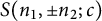in (9.22) into an $\alpha $ -sum modulo c (see (2.10)), the $\alpha $ - and $n_1$ -sums read

$$ \begin{align*} \sideset{}{^\star}\sum_{ \alpha (\mathrm{mod} \, c) } e \left ( \pm \frac {\overline{\alpha} h_2 n_2} {c} \right ) \sum_{n_1 \sim N_1 / d_1 } e \bigg( \frac {\alpha h_1 n_1} {c} + \frac {m_1 n_1} {c d_2 } \bigg) e \bigg( \frac {m_1 n_1} {c d_2 } \unicode{x3b3}_1 (r) \bigg) \textit{w} \bigg(\frac {d_1 n_1} {N_1} \bigg). \end{align*} $$

By applying the Poisson summation formula modulo $c d_2$ as in Lemma 6.1, this is turned into

(9.25) $$ \begin{align} \frac {N_1} {d_1} \, \sideset{}{^\star}\sum_{ \alpha (\mathrm{mod} \, c) } e \left ( \pm \frac {\overline{\alpha} h_2 n_2} {c} \right ) \sum_{n_1 \equiv - \alpha d_2 h_1 - m_1 (\mathrm{mod}\, c d_2)} \hat{\textit{w}} \bigg( \frac {N_1 (n_1 - m_1 \unicode{x3b3}_{1} (r))} {c d_1 d_2} \bigg). \end{align} $$

Note that the Fourier transform is negligibly small unless

(9.26) $$ \begin{align} | n_1-m_1 \unicode{x3b3}_1 (r) | < \frac {c d_1 d_2 T^{\varepsilon }} {N_1}. \end{align} $$

In view of (9.20) and (9.24),

so the $n_1$ -sum may be restricted effectively to the range . However, our assumption $ m_1 < \varPi /\varPi ^{\varepsilon } $ implies that only the zero frequency survives if we adjust $\varepsilon $ by our $\varepsilon $ -convention.

Given that $n_1 = 0$ , from (9.25) and (9.26), we obtain the congruence equation

$$ \begin{align*} \alpha d_2 h_1 \equiv - m_1 (\mathrm{mod}\, c d_2 ), \end{align*} $$

and the shrunk integral domain

(9.27) $$ \begin{align} | r | < \frac {c d_1 d_2 T^{\varepsilon }} {m_1 N_1 }. \end{align} $$

Note that the former has at most $ (c, h_1) $ many solutions of $\alpha $ modulo c. Moreover, a trivial estimation of the $n_2$ -sum yields a factor $O (N_2/d_2)$ . Consequently,

(9.28)

$Absolute value of script O sub plus-minus super plus-plus (r; c; d, h; N) is much less than the fraction with numerator N sub 1 N sub 2 (c, h sub 1) all over denominator d sub 1 d sub 2.$

Next, we insert this into (9.20) and bound the r-integral by $O (cd_1 d_2 T^{\varepsilon } / m_1 N_1)$ , which is the length of the new integral domain defined by (9.27). At any rate, we have

O plus plus sub plus minus (d, h; N) is much less than T epsilon dot Pi T dot N1 N2 all over d1 d2 dot d1 d2 all over m1 N1 summation over c much less than m1 N1 / d1 d2 T of (c, h1) which is much less than T epsilon Pi N1 N2 all over d1 d2.

Of course, the bound in the case $ m_1 N_1 < m_2 N_2 $ is the same, and hence

(9.29)

$Script O sub plus or minus (d, h; N) is much less than T to the epsilon power times the fraction with numerator Pi norm N all over denominator norm d.$

Thus, by (9.17) and (9.29), we conclude with the following estimate for .

Lemma 9.3 We have

(9.30)

9.4 Conclusion

In view of (9.1), Theorem 6 is a direct consequence of Lemmas 7.1, 9.2, and 9.3.

10 The mollified moments

Historically, the mollifier method was first used on zeros of the Riemann zeta function by Bohr, Landau, and Selberg [Reference Bohr and LandauBL, Reference SelbergSel]. In this section, we shall mainly follow the ideas and maneuvers in [Reference Iwaniec and SarnakIS, Reference Kowalski and MichelKM2].

10.1 Setup

We introduce the mollifier

(10.1) $$ \begin{align} M_f = \sum_{m \leqslant M} \frac {x_m \lambda_f (m)} {m^{1/2+it_f}}. \end{align} $$ upper M Subscript f Baseline equals sigma summation Underscript m less than or slanted equals upper M Endscripts StartFraction x Subscript m Baseline lamda Subscript f Baseline left parenthesis m right parenthesis Over m Superscript 1 divided by 2 plus i t Super Subscript f Superscript Baseline EndFraction period

Assume that the coefficients $ x_m $ are bounded, real-valued, and normalized so that

(10.2) $$ \begin{align} x_1 = 1, \end{align} $$

supported on square-free $m $ with $m \leqslant M$ . Note that

(10.3) $$ \begin{align} |M_f|^2 = \mathrm{Re} \mathop{\sum \sum}_{m_1, m_2 \leqslant M} \frac {x_{m_1} x_{m_2} \lambda_f (m_1) \lambda_f {(m_2)} } {\sqrt{m_1 m_2} (m_1/m_2)^{it_f} }. \end{align} $$

For $\unicode{x3D5} (t)$ given in (7.1), consider the mollified moments

(10.4)

(10.5)

By the Cauchy inequality,

(10.6) $$ \begin{align} \sideset{}{^{\delta}}\sum_{ L (s_f, f ) \neq 0} \omega_f \unicode{x3D5} (t_f) \geqslant \frac { \left| {\displaystyle \sideset{}{^{\delta}}\sum } \omega_f M_f L (s_f, f ) \unicode{x3D5} (t_f) \right|^2 } { {\displaystyle \sideset{}{^{\delta}}\sum } \omega_f \left|M_f L (s_f, f ) \right|^2 \unicode{x3D5} (t_f) } , \end{align} $$

StartLayout 1st Row sigma summation Underscript upper L left parenthesis s Subscript f Baseline comma f right parenthesis not equals 0 Overscript delta Endscripts omega Subscript f Baseline normal phi left parenthesis t Subscript f Baseline right parenthesis greater than or slanted equals StartFraction StartAbsoluteValue sigma summation Overscript delta Endscripts omega Subscript f Baseline upper M Subscript f Baseline upper L left parenthesis s Subscript f Baseline comma f right parenthesis normal phi left parenthesis t Subscript f Baseline right parenthesis EndAbsoluteValue squared Over sigma summation Overscript delta Endscripts omega Subscript f Baseline StartAbsoluteValue upper M Subscript f Baseline upper L left parenthesis s Subscript f Baseline comma f right parenthesis EndAbsoluteValue squared normal phi left parenthesis t Subscript f Baseline right parenthesis EndFraction comma EndLayout

where, of course, the $\delta $ indicates summation over . Our task is to calculate the mollified moments and and then carefully choose the coefficients $x_m$ to maximize the ratio .

10.2 The mollified first moment

By the definitions in (1.8), (10.1), and (10.4), we have

$M sub 1 super delta equals summation over m less than or equal to M of the fraction x sub m all over square root of m, times C sub 1 super delta (m).$

Thus, if we insert the asymptotic formula of in Theorem 5, then we obtain the main term $\varPi T /\pi \sqrt {\pi }$ , while, as $x_m$ are bounded, we estimate the error term by

Lemma 10.1 Let $\varPi = T^{ \nu }$ and $M = T^{\varDelta }$ . Then, for $\nu < 1$ and $\varDelta < (2\nu + 1)/3,$ there exists $\varepsilon = \varepsilon (\nu , \varDelta )> 0$ such that

(10.7)

10.3 The mollified second moment

In view of the definitions in (1.9), (10.3), and (10.5), we have

$M sub 2 super delta equals double summation over m sub 1, m sub 2 less than or equal to M of the fraction x sub m sub 1 x sub m sub 2 all over square root of m sub 1 m sub 2 times C sub 2 super delta (m sub 1, m sub 2).$

Assume that $ M < \varPi ^{1-\varepsilon }$ . Now we insert the asymptotic formula of 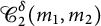in Theorem 6 and bound the error term by the sum of

and

Then, we arrive at the asymptotic formula for in the next lemma.

Lemma 10.2 Let $\varPi = T^{ \nu }$ and $M = T^{\varDelta }$ . Then, for $\nu < 1$ and $\varDelta < \min \{ 1/2, \nu \} $ , there exists $\varepsilon = \varepsilon (\nu , \varDelta )> 0$ such that

(10.8)

with

(10.9)

where $T_{\delta }$ is a multiple of T defined by

(10.10) $$ \begin{align} \log T_{\delta} = \log T + \gamma_{\delta}. \end{align} $$

By removing the co-primality condition $(m_1^{\star }, m_2^{\star }) = 1$ in (10.9) by the Möbius function, we have

By the definitions of $\sigma _{-1} (m)$ and $\sigma _{-1}' (m)$ in (1.14), some simple calculations yield

$$ \begin{align*} \sum_{d m = h} \frac{ \mu(d) \sigma_{-1} (m)}{d} = 1, \qquad \sum_{d m = h} \frac{ \mu(d) \sigma_{-1} (m )}{d} \log d + \sum_{d m = h} \frac{ \mu(d) \sigma_{-1}' (m )}{d} = 0. \end{align*} $$

Consequently,

(10.11)

$M sub 20 super delta equals triple summation over h, n sub 1, and n sub 2 of fraction x sub h n sub 1 times x sub h n sub 2 all over h n sub 1 n sub 2 times log of fraction T sub delta all over n sub 1 n sub 2.$

Thus, if we set

(10.12) $$ \begin{align} y_{h} = \sum_{n} \frac {x_{h n}} {n} , \qquad \breve{y}_h = \sum_{n} \frac {x_{h n} } {n} \log n , \end{align} $$

then (10.11) reads

(10.13)

By Möbius inversion, it follows from (10.12) that

(10.14) $$ \begin{align} x_n = \sum_{h} \frac { \mu (h)} {h} y_{h n}, \qquad \breve{y}_h = \sum_{n} \frac { \varLambda(n)} {n} y_{h n}, \end{align} $$ x Subscript n Baseline equals sigma summation Underscript h Endscripts StartFraction mu left parenthesis h right parenthesis Over h EndFraction y Subscript h n Baseline comma ModifyingAbove y With breve Subscript h Baseline equals sigma summation Underscript n Endscripts StartFraction upper Lamda left parenthesis n right parenthesis Over n EndFraction y Subscript h n Baseline comma

where $\varLambda (n) $ is the von Mangoldt function. Note that the assumption $x_1 = 1$ in (10.2) now becomes the linear constraint

(10.15) $$ \begin{align} \sum_{h} \frac { \mu (h)} {h} y_{h} = 1. \end{align} $$ sigma summation Underscript h Endscripts StartFraction mu left parenthesis h right parenthesis Over h EndFraction y Subscript h Baseline equals 1 period

By Cauchy, the optimal choice of $ y_{h} $ which minimizes the first quadratic form in (10.13) with respect to (10.15) is given by

(10.16) $$ \begin{align} y_h = \frac {\mu (h)} {\Xi (M) } , \qquad \Xi (M) = \sum_{h \leqslant M} \frac { \mu (h)^2 } {h}. \end{align} $$

We have

(10.17) $$ \begin{align} \Xi (M) = \frac {6} {\pi^2} \log M + O(1). \end{align} $$

Moreover, by (10.14) and (10.16), it is clear that our $x_{m}$ are indeed bounded.

By definition,

(10.18)

By the prime number theorem (see [Reference TitchmarshTit, Formula (3.14.3)]),

(10.19) $$ \begin{align} \sum_{ p \leqslant X} \frac { \log p } {p} = \log X + O (1), \end{align} $$ sigma summation Underscript p less than or slanted equals upper X Endscripts StartFraction log p Over p EndFraction equals log upper X plus upper O left parenthesis 1 right parenthesis comma

and, for h square-free,

(10.20) $$ \begin{align} \sum_{p | h} \frac {\log p} {p} = O (\log \log (3h)). \end{align} $$ sigma summation Underscript p vertical bar h Endscripts StartFraction log p Over p EndFraction equals upper O left parenthesis log log left parenthesis 3 h right parenthesis right parenthesis period

It follows from (10.14), (10.16), (10.19), and (10.20) that

$$ \begin{align*} {\breve{y}_h} /{y_h} = - \mathop{\sum_{p \nmid h }}_{ p \leqslant M/ h } \frac { \log p} { p } = - \log ( {M} /{h}) + O (\log \log (3 h)). \end{align*} $$

ModifyingAbove y With breve Subscript h Baseline divided by y Subscript h Baseline equals minus sigma summation Underscript p does not divide h Endscripts Underscript p less than or slanted equals upper M divided by h Endscripts StartFraction log p Over p EndFraction equals minus log left parenthesis upper M divided by h right parenthesis plus upper O left parenthesis log log left parenthesis 3 h right parenthesis right parenthesis period

Consequently,

and a partial summation using (10.17) yields

(10.21)

By (10.8), (10.13), (10.17), (10.18), and (10.21), we conclude with the following asymptotic formula for .

Lemma 10.3 Let $\varPi = T^{ \nu }$ and $M = T^{\varDelta }$ . Then, for $\varDelta < \min \{ 1/2, \nu \}, $ we have

(10.22)

10.4 Conclusion

For $0 < \nu < 1,$ let $\varPi = T^{ \nu }$ . By Lemmas 10.1 and 10.3, it follows from Cauchy in (10.6) that

(10.23) $$ \begin{align} \sideset{}{^{\delta}}\sum_{ L (s_f, f ) \neq 0} \omega_f \unicode{x3D5} (t_f) \geqslant \frac { \varPi T} {\pi \sqrt{\pi}} \bigg( \frac 6 {\pi^2} \min \bigg\{ \frac 1 3, \frac { \nu } { \nu + 1 } \bigg\} - \varepsilon \bigg) , \end{align} $$

as $T \rightarrow \infty $ for any $\varepsilon> 0$ . Next, we apply Lemma 5.1 with $a_n = \delta (L (s_f, f ) \neq 0)$ (namely, the Kronecker $\delta $ symbol) and $H = \varPi ^{1+\varepsilon }$ , obtaining

(10.24) $$ \begin{align} \mathop{\sideset{}{^{\delta}}\sum_{ |t_f - T| \leqslant H}}_{L (s_f, f ) \neq 0} \omega_f \geqslant \frac {2 H T} {\pi^2 } \bigg( \frac 6 {\pi^2} \min \bigg\{ \frac 1 3, \frac { \mu } { \mu + 1 } \bigg\} - \varepsilon \bigg) ,\qquad \mu = \frac {\log H} {\log T}, \end{align} $$

sigma summation Underscript StartAbsoluteValue t Subscript f Baseline minus upper T EndAbsoluteValue less than or slanted equals upper H Overscript delta Endscripts Underscript upper L left parenthesis s Subscript f Baseline comma f right parenthesis not equals 0 Endscripts omega Subscript f Baseline greater than or slanted equals StartFraction 2 upper H upper T Over pi squared EndFraction left parenthesis StartFraction 6 Over pi squared EndFraction min left brace one third comma StartFraction mu Over mu plus 1 EndFraction right brace minus epsilon right parenthesis comma mu equals StartFraction log upper H Over log upper T EndFraction comma

for any $ T^{ \varepsilon } \leqslant H \leqslant T/3$ . Recall the Weyl law (see (2.13)):

(10.25) $$ \begin{align} \sideset{}{^{\delta}}\sum_{ t_f \leqslant T} \omega_f = \frac {T^2} {2 \pi^2} + O (T); \end{align} $$ sigma summation Underscript t Subscript f Baseline less than or slanted equals upper T Overscript delta Endscripts omega Subscript f Baseline equals StartFraction upper T squared Over 2 pi squared EndFraction plus upper O left parenthesis upper T right parenthesis semicolon

as a consequence,

(10.26) $$ \begin{align} {\sideset{}{^{\delta}}\sum_{ |t_f - T| \leqslant H}} \omega_f = \frac {2 H T} {\pi^2 } + O (T). \end{align} $$ sigma summation Underscript StartAbsoluteValue t Subscript f Baseline minus upper T EndAbsoluteValue less than or slanted equals upper H Overscript delta Endscripts omega Subscript f Baseline equals StartFraction 2 upper H upper T Over pi squared EndFraction plus upper O left parenthesis upper T right parenthesis period

By (10.24)–(10.26), we deduce the following harmonic-weighted non-vanishing results.

Theorem 10.4 Let $\varepsilon> 0$ be arbitrarily small. As $T \rightarrow \infty $ , we have

(10.27) $$ \begin{align} \mathop{\sideset{}{^{\delta}}\sum_{ t_f \leqslant T}}_{L (s_f, f ) \neq 0} \omega_f \geqslant \bigg(\frac 2 {\pi^2} - \varepsilon \bigg) \sideset{}{^{\delta}}\sum_{ t_f \leqslant T} \omega_f , \end{align} $$

sigma summation Underscript t Subscript f Baseline less than or slanted equals upper T Overscript delta Endscripts Underscript upper L left parenthesis s Subscript f Baseline comma f right parenthesis not equals 0 Endscripts omega Subscript f Baseline greater than or slanted equals left parenthesis StartFraction 2 Over pi squared EndFraction minus epsilon right parenthesis sigma summation Underscript t Subscript f Baseline less than or slanted equals upper T Overscript delta Endscripts omega Subscript f Baseline comma

and, for $0 < \mu < 1$ ,

(10.28) $$ \begin{align} \mathop{\sideset{}{^{\delta}}\sum_{ |t_f - T| \leqslant T^{\mu}}}_{L (s_f, f ) \neq 0} \omega_f \geqslant \bigg( \frac {6} {\pi^2 } \min \bigg\{ \frac 1 3, \frac { \mu } { \mu + 1 } \bigg\} - \varepsilon \bigg)\, \sideset{}{^{\delta}}\sum_{ |t_f - T| \leqslant T^{\mu}} \omega_f , \end{align} $$

sigma summation Underscript StartAbsoluteValue t Subscript f Baseline minus upper T EndAbsoluteValue less than or slanted equals upper T Superscript mu Baseline Overscript delta Endscripts Underscript upper L left parenthesis s Subscript f Baseline comma f right parenthesis not equals 0 Endscripts omega Subscript f Baseline greater than or slanted equals left parenthesis StartFraction 6 Over pi squared EndFraction min left brace one third comma StartFraction mu Over mu plus 1 EndFraction right brace minus epsilon right parenthesis sigma summation Underscript StartAbsoluteValue t Subscript f Baseline minus upper T EndAbsoluteValue less than or slanted equals upper T Superscript mu Baseline Overscript delta Endscripts omega Subscript f Baseline comma

where the sums are over .

Note that (10.27) follows from (10.24) and (10.25) with $ H = T/3 $ along with a dyadic summation, while (10.28) follows directly from (10.24) and (10.26).

Since the harmonic weight

$$ \begin{align*} \omega_f = \frac {2} { L(1, \mathrm{Sym}^2 f )}, \end{align*} $$ omega Subscript f Baseline equals StartFraction 2 Over upper L left parenthesis 1 comma upper S y m squared f right parenthesis EndFraction comma

one may remove $\omega _f$ without compromising the strength of results by the method of Kowalski and Michel [Reference Kowalski and MichelKM1], adapted for the Maass-form case in [Reference Balkanova, Huang and SödergrenBHS] (see also the paragraph below (2.9) in [Reference Iwaniec and SarnakIS]). Thus, after the removal of $\omega _f$ , we obtain the non-vanishing results in Theorems 1 and 2.

11 Moments with no twist and smooth weight

Theorem 11.1 Let $ T^{ \varepsilon } \leqslant H \leqslant T/3$ . Then,

(11.1) $$ \begin{align} \sideset{}{^{\delta}}\sum_{ |t_f - T| \leqslant H } \omega_f L (s_f, f ) = \frac { 2 } {\pi^2} H T + O \big(T^{ \varepsilon } ( H \sqrt{T} + T ) \big). \end{align} $$

Proof By applying Lemma 5.1 to the first asymptotic formula in Corollary 7, we have

$$ \begin{align*} \sideset{}{^{\delta}}\sum_{ |t_f - T| \leqslant H } \omega_f L (s_f, f ) = \frac { 2 } {\pi^2} H T + O \big(T^{\varepsilon } (H \sqrt{T} + \varPi T) \big), \end{align*} $$

for any $T^{\varepsilon } \leqslant \varPi ^{1+\varepsilon } \leqslant H \leqslant T / 3 $ , and we obtain (11.1) on the choice $ \varPi = H / \sqrt {T} + T^{\varepsilon } $ .

Theorem 11.2 Let $ T^{ \varepsilon } \leqslant H \leqslant T/3$ . Then,

(11.2) $$ \begin{align} \sideset{}{^{\delta}}\sum_{ |t_f - T| \leqslant H } \omega_f |L (s_f, f )|^2 = \frac {1} {\pi^2} \! \int_{T-H}^{T+H} K ( \log K + \gamma_{\delta}) \mathrm{d} K + O \big(T^{ \varepsilon } ( {\textstyle H \sqrt{T} + \sqrt{H} T} ) \big). \end{align} $$

Proof By applying Lemma 5.1 to the second asymptotic formula in Corollary 7, we infer that the spectral second moment on the left of (11.2) equals

$$ \begin{align*} \frac {1} {\pi^2} \int_{T-H}^{T+H} K ( \log K + \gamma_{\delta}) \mathrm{d} K + O \bigg(T^{\varepsilon } \bigg(H\sqrt{T} + \frac {H T } {\varPi } + \varPi T \bigg)\bigg), \end{align*} $$

for any $\varPi ^{1+\varepsilon } \leqslant H \leqslant T/3$ , and we obtain (11.2) on the choice $\varPi = \sqrt {H}$ .

Corollary 8 is a direct consequence of the above asymptotics with $H = T/3$ along with a dyadic summation.

Part II

Density theorems

12 Sums of variant Kloosterman sums

Let us introduce the variant Kloosterman sum

(12.1) $$ \begin{align} V_{q} (m, n; c) = \mathop{\sum_{\alpha (\mathrm{mod}\, c)}}_{ (\alpha (q-\alpha ), c) = 1 } e \bigg( \frac { \overline{\alpha } m + \overline{(q - \alpha) } n } {c} \bigg). \end{align} $$

StartLayout 1st Row upper V Subscript q Baseline left parenthesis m comma n semicolon c right parenthesis equals sigma summation Underscript alpha left parenthesis mod c right parenthesis Endscripts Underscript left parenthesis alpha left parenthesis q minus alpha right parenthesis comma c right parenthesis equals 1 Endscripts e left parenthesis StartFraction ModifyingAbove alpha With quotation dash m plus ModifyingAbove left parenthesis q minus alpha right parenthesis With quotation dash n Over c EndFraction right parenthesis period EndLayout

The definition of $V_{q} (m, n; c)$ is essentially from Iwaniec and Li [Reference Iwaniec and LiIL, Formula (2.17)] and arose in the identity of Luo [Reference LuoLuo2, Section 3]:

(12.2) $$ \begin{align} S (m, n; c) e \Big(\frac {m+n} {c} \Big) = \sum_{r q = c } V_{q} (m, n; r). \end{align} $$ upper S left parenthesis m comma n semicolon c right parenthesis e left parenthesis StartFraction m plus n Over c EndFraction right parenthesis equals sigma summation Underscript r q equals c Endscripts upper V Subscript q Baseline left parenthesis m comma n semicolon r right parenthesis period

The purpose of this section is to prove the following analog of [Reference Iwaniec, Luo and SarnakILS, Lemma 6.1].

Lemma 12.1 Assuming the Riemann hypothesis for Dirichlet L-functions, for any $x \geqslant 2$ , we have

(12.3) $$ \begin{align} \mathop{\sum_{p \leqslant x} }_{p \nmid c} V_{q} (m p, n; c) \log p = \frac {x} {\varphi (c)} R (m; c) R_q (n; c) + O (\varphi (c) \sqrt{x} \log^2 (cx) ) , \end{align} $$

StartLayout 1st Row sigma summation Underscript p less than or slanted equals x Endscripts Underscript p does not divide c Endscripts upper V Subscript q Baseline left parenthesis m p comma n semicolon c right parenthesis log p equals StartFraction x Over phi left parenthesis c right parenthesis EndFraction upper R left parenthesis m semicolon c right parenthesis upper R Subscript q Baseline left parenthesis n semicolon c right parenthesis plus upper O left parenthesis phi left parenthesis c right parenthesis StartRoot x EndRoot log squared left parenthesis c x right parenthesis right parenthesis comma EndLayout

where $\varphi (c) $ is the Euler function, $R (m; c) = S (m, 0; c)$ , and $R_q (n; c) = V_q (0, n; c) $ .

Proof As in [Reference Iwaniec, Luo and SarnakILS, Section 6], we shall use the Riemann hypothesis for Dirichlet L-functions in the form

$$ \begin{align*} \sum_{p \leqslant x} \chi (p) \log p = \delta ({\chi }) \cdot x + O (\sqrt{x} \log^2 (c x)), \end{align*} $$

where $ \chi $ is any character to modulus c and $\delta ({\chi })$ is the indicator of the principal character. By definition,

$$ \begin{align*} \sum_{\alpha (\mathrm{mod}\, c)} \chi (\alpha) V_q (\alpha m, n; c) = \mathop{\mathop{\sum \sum}_{\alpha, \beta (\mathrm{mod}\, c)}}_{(\beta(q -\beta), c) = 1} \chi (\alpha) e \bigg( \frac { \alpha \overline{\beta } m + \overline{(q - \beta ) } n } {c} \bigg) , \end{align*} $$

StartLayout 1st Row sigma summation Underscript alpha left parenthesis mod c right parenthesis Endscripts chi left parenthesis alpha right parenthesis upper V Subscript q Baseline left parenthesis alpha m comma n semicolon c right parenthesis equals sigma summation sigma summation Underscript alpha comma beta left parenthesis mod c right parenthesis UnderUnderscript left parenthesis beta left parenthesis q minus beta right parenthesis comma c right parenthesis equals 1 Endscripts chi left parenthesis alpha right parenthesis e left parenthesis StartFraction alpha ModifyingAbove beta With quotation dash m plus ModifyingAbove left parenthesis q minus beta right parenthesis With quotation dash n Over c EndFraction right parenthesis comma EndLayout

and, on the change $ \alpha \rightarrow \alpha \beta , $ it splits into the product $ G (m; \chi ) G_{ q} (n; \chi )$ with

$$ \begin{align*} G (m; \chi ) = \sum_{\alpha (\mathrm{mod}\, c)} \chi (\alpha) e \Big( \frac { \alpha m } {c} \Big) , \qquad G_{ q} (n; \chi ) = \mathop{\sum_{\alpha (\mathrm{mod}\, c)}}_{ ( q-\alpha , c) = 1 } \chi (\alpha) e \bigg( \frac { \overline{(q - \alpha) } n } {c} \bigg). \end{align*} $$

StartLayout 1st Row upper G left parenthesis m semicolon chi right parenthesis equals sigma summation Underscript alpha left parenthesis mod c right parenthesis Endscripts chi left parenthesis alpha right parenthesis e left parenthesis StartFraction alpha m Over c EndFraction right parenthesis comma upper G Subscript q Baseline left parenthesis n semicolon chi right parenthesis equals sigma summation Underscript alpha left parenthesis mod c right parenthesis Endscripts Underscript left parenthesis q minus alpha comma c right parenthesis equals 1 Endscripts chi left parenthesis alpha right parenthesis e left parenthesis StartFraction ModifyingAbove left parenthesis q minus alpha right parenthesis With quotation dash n Over c EndFraction right parenthesis period EndLayout

Note that for the principal character, these (Gauss) sums become the (Ramanujan) sums $R (m; c)$ and $R_q (n; c)$ , and that by the orthogonality of characters,

$$ \begin{align*} \sum_{\chi (\mathrm{mod}\, c)} |G (m; \chi )|^2 = R (0; c)^2 , \qquad \sum_{\chi (\mathrm{mod}\, c)} |G_{ q} (m; \chi )|^2 = R (0; c) R_q (0; c). \end{align*} $$

Finally, from these formulas, we derive

$$ \begin{align*} \mathop{\sum_{p \leqslant x} }_{p \nmid c} \! V_{q} (m p, n; c) \log p & = \frac 1 {\varphi (c)} \! \sum_{\chi (\mathrm{mod}\, c)} \! \bigg( \sum_{\alpha (\mathrm{mod}\, c)} \! \! \chi (\alpha) V_q (\alpha m, n; c) \bigg) \bigg( \sum_{p \leqslant x} \overline{\chi } (p) \log p \bigg)\\ & = \frac 1 {\varphi (c)} \! \sum_{\chi (\mathrm{mod}\, c)} \! G (m; \chi ) G_{ q} (n; \chi ) \big( \delta {(\chi )} \cdot x + O (\sqrt{x} \log^2 (c x)) \big), \end{align*} $$

StartLayout 1st Row 1st Column sigma summation Underscript p less than or slanted equals x Endscripts Underscript p does not divide c Endscripts upper V Subscript q Baseline left parenthesis m p comma n semicolon c right parenthesis log p 2nd Column equals StartFraction 1 Over phi left parenthesis c right parenthesis EndFraction sigma summation Underscript chi left parenthesis mod c right parenthesis Endscripts left parenthesis sigma summation Underscript alpha left parenthesis mod c right parenthesis Endscripts chi left parenthesis alpha right parenthesis upper V Subscript q Baseline left parenthesis alpha m comma n semicolon c right parenthesis right parenthesis left parenthesis sigma summation Underscript p less than or slanted equals x Endscripts ModifyingAbove chi With quotation dash left parenthesis p right parenthesis log p right parenthesis 2nd Row 1st Column Blank 2nd Column equals StartFraction 1 Over phi left parenthesis c right parenthesis EndFraction sigma summation Underscript chi left parenthesis mod c right parenthesis Endscripts upper G left parenthesis m semicolon chi right parenthesis upper G Subscript q Baseline left parenthesis n semicolon chi right parenthesis left parenthesis delta left parenthesis chi right parenthesis dot x plus upper O left parenthesis StartRoot x EndRoot log squared left parenthesis c x right parenthesis right parenthesis right parenthesis comma EndLayout

and hence (12.3).

Later in our application, $m = 1$ and $n = \pm 1$ . It is well known that the Ramanujan sum

(12.4) $$ \begin{align} R (1; c) = \mu (c). \end{align} $$

By the Chinese remainder theorem, it is easy to prove

(12.5) $$ \begin{align} R_q (\pm 1; c) = O \big( \tau (c) \mu (c)^2 \big). \end{align} $$

13 Further analysis for the Bessel integrals

Set $\unicode{x3b3} (t) \equiv 1$ in (4.3) so that

$$ \begin{align*} h_2 (t; y) = 2 \cos (2 t \log y) (\unicode{x3D5} (t) + \unicode{x3D5} (-t)). \end{align*} $$

According to (4.4) and (4.7), up to a negligible error, we split $H_2^{\pm } (x, y) $ into four similar parts, one of which reads

(13.1) $$ \begin{align} \frac {\exp (- i (v \pm w) ) \cdot I^{_\pm}_{^{- +} } (v, w)} 2 , \qquad v = \frac {xy} {2}, \quad w = \frac {x/y} 2, \end{align} $$

with

(13.2) $$ \begin{align} I^{_\pm}_{^{- +} } (v, w) = \varPi T \int_{-\varPi^{\varepsilon }/\varPi}^{\varPi^{\varepsilon }/ \varPi} g ( \varPi r) \exp ( 2 i T r - i (\unicode{x3c1}(r) v \pm \unicode{x3c1} (-r) w ) ) \mathrm{d} r , \end{align} $$

for $ \unicode{x3c1} (r) = \exp (r) - 1. $ More explicitly, the pair of $\pm $ in the subscript of $I^{_\pm }_{^{\pm \pm } } (v, w) $ is determined by that in $ \pm i \unicode{x3c1} (\pm r) v $ contained in the integral. Later, we shall have

$$ \begin{align*} x = \frac {4\pi \sqrt{p}} {c}, \qquad y = \sqrt{p}, \end{align*} $$

and

$$ \begin{align*} v = \frac {2\pi p} {c}, \qquad w = \frac {2\pi} {c}; \end{align*} $$

so, in practice, $w $ is small and inessential and will be suppressed from the notation.

Lemma 13.1 Write

(13.3) $$ \begin{align} I^{_{\pm \natural}}_{^{- +} } (v, w) = \frac { \partial I^{_\pm}_{^{-+} } (v, w) } {\partial v}. \end{align} $$

Then, we have bounds

(13.4)

Moreover, if $ w < \varPi $ , then $I^{_\pm }_{^{-+} } (v, w), I^{_{\pm \natural }}_{^{-+} } (v, w) = O (T^{-A})$ unless .

Proof Note that $I^{_{\pm \natural }}_{^{-+} } (v, w) $ is very similar to $I^{_{\pm }}_{^{-+} } (v, w) $ :

(13.5) $$ \begin{align} I^{_{\pm \natural}}_{^{-+} } (v, w) = - i \varPi T \int_{-\varPi^{\varepsilon }/\varPi}^{\varPi^{\varepsilon }/ \varPi} g ( \varPi r) \cdot \unicode{x3c1} (r) \exp ( 2 i T r - i (\unicode{x3c1}(r) v \pm \unicode{x3c1} (-r) w ) ) \mathrm{d} r. \end{align} $$

Clearly, (13.4) follows from (13.2) and (13.5) by trivial estimation. As for the second statement, we use the method of stationary phase. By $w < \varPi $ , we may as well absorb the factor $ \exp (\mp i \unicode{x3c1} (-r)w)$ into the weight $g (\varPi r)$ so that the phase function is $ 2 T r - \unicode{x3c1} (r) v $ , while its derivative equals

$$ \begin{align*} 2 T - \exp(r) v = 2 T - v + O ( v \varPi^{\varepsilon }/ \varPi ). \end{align*} $$

Thus, in the case , by an application of Lemma B.1 in [Reference QiQi] with $S = 1$ , $ P = 1/\varPi $ , $Q = 1$ , $Z = T $ , and $ R = \varPi ^{\varepsilon } ( \varPi +T / \varPi ) $ , we infer that the integrals in (13.2) and (13.5) are negligibly small. Note here that $R $ is larger than both $ \varPi ^{1+\varepsilon }$ and $ T^{1/2+\varepsilon }$ . However, for 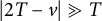, the integrals are always negligibly small if we apply Lemma B.1 in [Reference QiQi] with $S = 1$ , $ P = 1/\varPi $ , $Q = 1$ , $Z = v$ , and $ R = v + T $ .

Remark 13.1 As for the other three integrals $I^{_\pm }_{^{+-} } (v, w) $ , $I^{_\pm }_{^{+ +} } (v, w) $ , and $I^{_\pm }_{^{- -} } (v, w) $ , the first one is similar, while the latter two are always negligible.

14 The explicit formula

By applying [Reference Rudnick and SarnakRS, Proposition 2.1] with

$$ \begin{align*} g (u) = \frac 1 {\log T} {e \left ( - \frac { u t_f } {2\pi} \right )} \hat{\unicode{x3c6}} \bigg( \frac {u} {\log T}\bigg), \qquad h (r) = \unicode{x3c6} \bigg(\frac {\log T} {2\pi} (r-t_f) \bigg), \end{align*} $$

we obtain the explicit formula

(14.1) $$ \begin{align} D (f; \unicode{x3c6}; T) = H (f; \unicode{x3c6}; T) - P (f; \unicode{x3c6}; T), \end{align} $$

with

(14.2) $$ \begin{align} D (f; \unicode{x3c6}; T) = \sum_{\gamma_f } \unicode{x3c6} \bigg(\frac {\log T} {2\pi} (\gamma_f-t_f) \bigg) , \end{align} $$ upper D left parenthesis f semicolon phi semicolon upper T right parenthesis equals sigma summation Underscript gamma Subscript f Baseline Endscripts phi left parenthesis StartFraction log upper T Over 2 pi EndFraction left parenthesis gamma Subscript f Baseline minus t Subscript f Baseline right parenthesis right parenthesis comma

as defined before in (1.19), and

(14.3) $$ \begin{align} H ( f; \unicode{x3c6}; T) = \frac 1 {\pi} \! \int_{-\infty}^{\infty} \! \! \unicode{x3c6} \bigg(\frac {\log T} {2\pi} r \bigg) \bigg\{ \frac {\Gamma_{\mathbf{R}}' } {\Gamma_{\mathbf{R}} } \big(2\kappa _f + i r \big) + \mathrm{Re}\, \frac {\Gamma_{\mathbf{R}}' } {\Gamma_{\mathbf{R}} } \big(2\kappa _f + 2 it_f + ir \big) \bigg\} \mathrm{d} r , \end{align} $$

(14.4) $$ \begin{align} P (f; \unicode{x3c6}; T) = 2 \sum_{n=1}^{\infty} \frac {\Lambda (n) a_f (n) \cos (t_f \log n)} { \sqrt{n} \, {\log T} } \hat{\unicode{x3c6}} \bigg( \frac {\log n} {\log T}\bigg), \end{align} $$

where

$$ \begin{align*} \kappa _f = \frac {1+2\delta_f} {4} \end{align*} $$

(see (3.3) and (3.4)), as usual, $\Gamma _{\mathbf {R}} (s) = \pi ^{-s/2} \Gamma (s/2) $ , $\Lambda (n) $ is the von Mangoldt function ( $\Lambda (n) = \log p$ 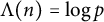if $n = p^{\nu }$ and $0$ otherwise), and

$$ \begin{align*} a_f (p^{\nu } ) = \alpha_f (p)^{\nu } + \beta_f (p)^{\nu }, \end{align*} $$

for $\alpha _f (p)$ and $ \beta _f (p)$ defined as in the Euler product (3.6).

Lemma 14.1 Let $\mathrm {Re} (s) \geqslant \delta> 0$ . Then, for , we have

(14.5) $$ \begin{align} \frac 1 {\pi} \int_{-\infty}^{\infty} \unicode{x3c6} \bigg(\frac {\log T} {2\pi} r \bigg) \frac {\Gamma_{\mathbf{R}}' } {\Gamma_{\mathbf{R}} } ( 2 s + i r ) \mathrm{d} r = \frac {\log (s/\pi)} {\log T} \hat{\unicode{x3c6}} (0) + O_{\delta} \bigg(\frac 1 { \log T} \bigg). \end{align} $$

Proof By definition, $\Gamma _{\mathbf {R}} (s) = \pi ^{-s/2} \Gamma (s/2) $ , and by the change $r \rightarrow 2\pi r/ \log T$ , the integral in (14.5) is turned into

$$ \begin{align*} \frac {1} {\log T} \int_{-\infty}^{\infty} \unicode{x3c6} (r) \left ( \frac {\Gamma'} {\Gamma } \bigg( s + \frac { \pi i r } {\log T} \bigg) -\log \pi \right ) \mathrm{d} r. \end{align*} $$ StartFraction 1 Over log upper T EndFraction integral Subscript negative infinity Superscript infinity Baseline phi left parenthesis r right parenthesis left parenthesis StartFraction normal upper Gamma prime Over normal upper Gamma EndFraction left parenthesis s plus StartFraction pi i r Over log upper T EndFraction right parenthesis minus log pi right parenthesis normal d r period

It follows from the Stirling formula

$$ \begin{align*} \frac {\Gamma'(s)} {\Gamma (s) }= \log s + O \left ( \frac 1 {|s|} \right ), \end{align*} $$ StartLayout 1st Row StartFraction normal upper Gamma prime left parenthesis s right parenthesis Over normal upper Gamma left parenthesis s right parenthesis EndFraction equals log s plus upper O left parenthesis StartFraction 1 Over StartAbsoluteValue s EndAbsoluteValue EndFraction right parenthesis comma EndLayout

and the crude uniform bound

$$ \begin{align*} \log (s + w) - \log s = O_{\delta} \left ( \left|\frac {w} {s} \right| \log (|w|+2) \right ), \qquad (\mathrm{Re}(s) \geqslant \delta> 0, \, \mathrm{Re}(w) \geqslant 0) , \end{align*} $$

that the integral above equals

$$ \begin{align*} & \frac {1} {\log T} \int_{-\infty}^{\infty} \unicode{x3c6} (r) \log \bigg( \frac s {\pi} + \frac { i r } {\log T} \bigg) \mathrm{d} r + O \bigg(\frac 1 { \log T} \bigg) \\ &\quad = \frac {1} {\log T} \int_{-\infty}^{\infty} \unicode{x3c6} (r) \bigg(\log \left ( \frac s {\pi} \right ) + O \bigg(\frac {|r| \log (|r|+2)} {|s| \log T} \bigg) \bigg) \mathrm{d} r + O \bigg(\frac 1 { \log T} \bigg) \\ &\quad = \frac {\log (s/\pi) } {\log T} \int_{-\infty}^{\infty} \unicode{x3c6} (r) \mathrm{d} r + O \bigg(\frac 1 { \log T} \bigg), \end{align*} $$

StartLayout 1st Row 1st Column Blank 2nd Column StartFraction 1 Over log upper T EndFraction integral Subscript negative infinity Superscript infinity Baseline phi left parenthesis r right parenthesis log left parenthesis StartFraction s Over pi EndFraction plus StartFraction i r Over log upper T EndFraction right parenthesis normal d r plus upper O left parenthesis StartFraction 1 Over log upper T EndFraction right parenthesis 2nd Row 1st Column Blank 2nd Column equals StartFraction 1 Over log upper T EndFraction integral Subscript negative infinity Superscript infinity Baseline phi left parenthesis r right parenthesis left parenthesis log left parenthesis StartFraction s Over pi EndFraction right parenthesis plus upper O left parenthesis StartFraction StartAbsoluteValue r EndAbsoluteValue log left parenthesis StartAbsoluteValue r EndAbsoluteValue plus 2 right parenthesis Over StartAbsoluteValue s EndAbsoluteValue log upper T EndFraction right parenthesis right parenthesis normal d r plus upper O left parenthesis StartFraction 1 Over log upper T EndFraction right parenthesis 3rd Row 1st Column Blank 2nd Column equals StartFraction log left parenthesis s divided by pi right parenthesis Over log upper T EndFraction integral Subscript negative infinity Superscript infinity Baseline phi left parenthesis r right parenthesis normal d r plus upper O left parenthesis StartFraction 1 Over log upper T EndFraction right parenthesis comma EndLayout

as desired.

Remark 14.1 By modifying the proof of Lemma 14.1, one may improve the error term $O_{\delta } (1/\log T)$ 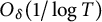into $ O_{\delta , \varepsilon } (1 / |s| \log T) $ if .

By applying Lemma 14.1 with $s = \kappa _f$ or $s = \kappa _f + it_f$ to (14.3), we have

(14.6) $$ \begin{align} H ( f; \unicode{x3c6}; T) = \frac {\log |\kappa _f + it_f| } {\log T} \hat{\unicode{x3c6}} (0) + O \bigg(\frac 1 { \log T} \bigg). \end{align} $$ upper H left parenthesis f semicolon phi semicolon upper T right parenthesis equals StartFraction log StartAbsoluteValue kappa Subscript f Baseline plus i t Subscript f Baseline EndAbsoluteValue Over log upper T EndFraction ModifyingAbove phi With caret left parenthesis 0 right parenthesis plus upper O left parenthesis StartFraction 1 Over log upper T EndFraction right parenthesis period

Lemma 14.2 Assume the Riemann hypothesis (for the Riemann zeta function). Let $ s = 1 + it $ and . Then,

(14.7) $$ \begin{align} \sum_{p < x} \frac {\log p} {p^s} = O( \log \log t), \end{align} $$ sigma summation Underscript p less than x Endscripts StartFraction log p Over p Superscript s Baseline EndFraction equals upper O left parenthesis log log t right parenthesis comma

for $ x < t$ , where the implied constant is absolute.

Proof As usual, write $s = \sigma + it$ . By [Reference TitchmarshTit, Sections 14.5 and 14.33], under the Riemann hypothesis, we have

(14.8) $$ \begin{align} \frac {\zeta' (s)} {\zeta (s)} = O \big( ({\log t})^{2-2\sigma} \big), \end{align} $$ StartLayout 1st Row StartFraction zeta prime left parenthesis s right parenthesis Over zeta left parenthesis s right parenthesis EndFraction equals upper O left parenthesis left parenthesis log t right parenthesis Superscript 2 minus 2 sigma Baseline right parenthesis comma EndLayout

uniformly for $1/2 < \sigma _0 \leqslant \sigma \leqslant \sigma _1 < 1$ , while

(14.9) $$ \begin{align} \frac {\zeta' (s)} {\zeta (s)} = O (\log \log t), \end{align} $$ StartLayout 1st Row StartFraction zeta prime left parenthesis s right parenthesis Over zeta left parenthesis s right parenthesis EndFraction equals upper O left parenthesis log log t right parenthesis comma EndLayout

for $ \sigma = 1$ . By (14.8), it follows from the Perron formula in [Reference TitchmarshTit, Lemma 3.12] and the contour-shift argument in [Reference TitchmarshTit, Sections 3.14 and 3.15] with $c = 1/ \log x$ and $\delta = 1 - \sigma _0 $ that

$$ \begin{align*} \sum_{n < x} \frac {\Lambda (n)} {n^{s}} + \frac {\zeta' (s)} {\zeta (s)} - \frac {x^{1-s}} {1-s} = O \bigg( \frac {\log^2 x} {T} + \frac {\log T \cdot \log^{ 2\delta} t} {x^{\delta}} + \frac {\log^{2 \delta} t} {T} \bigg) , \end{align*} $$

in the case that $\sigma = 1$ and $T < t/2$ ; here, one may let x be half-integral. For $x < t$ , on choosing $\sqrt {T} = \log x + \log ^{\delta } t$ , we obtain

(14.10) $$ \begin{align} \sum_{p < x} \frac {\log p} {p^{s}} + \frac {\zeta' (s)} {\zeta (s)} = O \bigg( 1 + \frac {\log \log t \cdot \log^{ 2\delta} t} {x^{\delta}} \bigg). \end{align} $$

Note here that

$$ \begin{align*} \sum_{n < x} \frac {\Lambda (n)} {n^{s}} = \sum_{p < x} \frac {\log p} {p^s} + O (1). \end{align*} $$ sigma summation Underscript n less than x Endscripts StartFraction normal upper Lamda left parenthesis n right parenthesis Over n Superscript s Baseline EndFraction equals sigma summation Underscript p less than x Endscripts StartFraction log p Over p Superscript s Baseline EndFraction plus upper O left parenthesis 1 right parenthesis period

Also, trivially, we have

(14.11) $$ \begin{align} \sum_{p < x} \frac {\log p} {p^{s}} = O (\log x). \end{align} $$ sigma summation Underscript p less than x Endscripts StartFraction log p Over p Superscript s Baseline EndFraction equals upper O left parenthesis log x right parenthesis period

Accordingly, as $x> \log ^2 t$ or not, the bound (14.7) follows from (14.9), (14.10), or (14.11).

Now we turn to the sum $P ( f; \unicode{x3c6}; T)$ as defined in (14.4): unlike the cases of central L-values in [Reference Alpoge and MillerAM, Reference Iwaniec, Luo and SarnakILS, Reference Liu and QiLQ1], this will not contribute a main term. Suppose that $\hat {\unicode{x3c6} }$ has support in $(-2, 2)$ , say, and $ t_f $ is close to T.

Firstly, we may discard those terms with $n = p^{\nu }$ for $\nu \geqslant 3$ since $|a_f (p^{\nu }) | \leqslant 2 p^{\frac 7 {64} \nu }$ 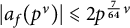by the Kim–Sarnak bound (3.7), and hence their contribution is $O (1/\log T)$ . Next, by partial summation, it follows from Lemma 14.2 that

(14.12) $$ \begin{align} \sum_{p} \frac { \cos (2 t_f \log p ) \log p} {p \log T} \hat{\unicode{x3c6}} \bigg(\frac {2 \log p} {\log T} \bigg) = O_{\unicode{x3c6}} \bigg( \frac {\log \log T} {\log T} \bigg). \end{align} $$

Since $a_f (p) = \lambda _{f} (p)$ 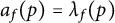and $ a_f (p^2) = \lambda _{f} (p^2) - 1 $ , we conclude that

(14.13) $$ \begin{align} P ( f; \unicode{x3c6}; T) = P_1 (f; \unicode{x3c6}; T) + P_2 (f; \unicode{x3c6}; T) + O_{\unicode{x3c6}} \bigg( \frac {\log \log T} {\log T} \bigg) , \end{align} $$

with

(14.14) $$ \begin{align} P_{\nu } (f; \unicode{x3c6}; T) = 2 \sum_{p} \lambda_f (p^{\nu }) \frac {\cos (\nu t_f \log p ) \log p} {p^{\nu /2} \log T} \hat{\unicode{x3c6}} \bigg(\frac {\nu \log p} {\log T} \bigg). \end{align} $$

Finally, we obtain the following asymptotic formula by combining (14.1), (14.6), and (14.13).

Lemma 14.3 We have

(14.15) $$ \begin{align} D (f; \unicode{x3c6}; T) \!= \! \frac {\log |\kappa _f + it_f| } {\log T} \hat{\unicode{x3c6}} (0) - P_1 (f; \unicode{x3c6}; T) - P_2 (f; \unicode{x3c6}; T) + O_{\unicode{x3c6}} \! \bigg( \frac {\log \log T} {\log T} \bigg) , \end{align} $$

if $\hat {\unicode{x3c6} }$ has support in $(-2, 2)$ .

15 Proof of the density theorems

As in (4.2), let us define

(15.1) $$ \begin{align} \unicode{x3D5} (t) = \unicode{x3D5}_{T, \varPi} (t) = \exp \left( - \frac {(t-T)^2} {\varPi^2} \right)\!, \end{align} $$ StartLayout 1st Row normal phi left parenthesis t right parenthesis equals normal phi Subscript upper T comma upper Pi Baseline left parenthesis t right parenthesis equals exp left parenthesis minus StartFraction left parenthesis t minus upper T right parenthesis squared Over upper Pi squared EndFraction right parenthesis comma EndLayout

and consider the -averaged $1$ -level density

(15.2)

Clearly, 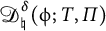differs from 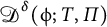as in (1.20) only by an exponentially small error term. By inserting (14.15), we have

(15.3)

with

(15.4)

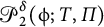
Note here that the main term $ \varPi T \hat {\unicode{x3c6} } (0) / \pi \sqrt {\pi } $ 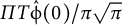is due to the Weyl law as in (2.13). Therefore, Theorems 9 and 10 are deducible easily from the following bounds for 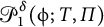and .

Lemma 15.1 We have

(15.5)

if $\hat {\unicode{x3c6} }$ has support in $(-1, 1)$ .

Lemma 15.2 Let $\varPi = T^{\mu }$ for $0 < \mu < 1$ . Assume the Riemann hypothesis for Dirichlet L-functions. Define

(15.6) $$ \begin{align} v (\mu) = \left\{ \begin{aligned} & 1, & & \text{ if }\ 0 < \mu \leqslant 1/3,\\ & 3 \mu, & & \text{ if }\ 1/3 < \mu \leqslant 1/2, \\ & 1 + \mu, & & \text{ if }\ 1/2 < \mu < 1. \end{aligned}\right. \end{align} $$

v left parenthesis mu right parenthesis equals StartLayout Enlarged left brace 1st Row 1st Column Blank 2nd Column 1 comma 3rd Column Blank 4th Column if 0 less than mu less than or slanted equals 1 divided by 3 comma 2nd Row 1st Column Blank 2nd Column 3 mu comma 3rd Column Blank 4th Column if 1 divided by 3 less than mu less than or slanted equals 1 divided by 2 comma 3rd Row 1st Column Blank 2nd Column 1 plus mu comma 3rd Column Blank 4th Column if 1 divided by 2 less than mu less than 1 period EndLayout

Then, we have

(15.7)

if $\hat {\unicode{x3c6} }$ has support in $(- v(\mu ), v (\mu ))$ .

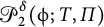
Subsequently, we shall focus on 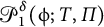as the treatment of is much easier and yields a better bound.

Notation

Suppose $\hat {\unicode{x3c6} }$ has support in the closed interval $ [-v, v] $ , say for $v < 2$ . Let $\varPi = T^{\mu }$ and $P = T^{v}$ .

For brevity, let us write $ \unicode{x3D5} (t) = \unicode{x3D5} _{T, \varPi } (t)$ as before and suppress $T, \varPi $ from the notation like .

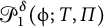15.1 Application of the Kuznetsov formula

By (14.14) and (15.4), we may write

where, as in (4.3),

$$ \begin{align*} h_2 (t; y) = 2 \cos (2t \log y) (\unicode{x3D5} (t) + \unicode{x3D5} (-t)). \end{align*} $$

By applying the Kuznetsov trace formula in (2.9), we have

(15.8)

where

(15.9)

(15.10)

First of all, the Eisenstein term is indeed small. Since the integral in (15.9) is trivially $O (\varPi \log ^2 T)$ 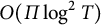(by [Reference TitchmarshTit, (3.11.10)]), we have

(15.11)

Note that the similar Eisenstein term is even smaller: $ O (\varPi \log ^2 T) $ .

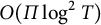It is now left to consider the off-diagonal sums as in (15.10).

15.2 Proof of Lemma 15.1

It follows from Corollary 4.1 that the Bessel integral $ H_2^{\pm } ( {4\pi \sqrt {p}} / {c} , \sqrt {p} )$ in (15.10) is negligibly small for . Therefore, is negligible for $v < 1$ so that $ p / T = o (1) $ for all $p \leqslant P = T^{v}$ . Similarly, the off-diagonal contribution to is also negligible for $v < 1$ .

Note that, in the odd case, and are actually negligibly small as there is no Eisenstein contribution.

15.3 Proof of Lemma 15.2

In light of (15.8) and (15.11), it suffices to prove for any $v < v (\mu )$ . As in Section 13, let us split into four similar parts, one of which contains $ I^{_\pm }_{^{- +} } (2\pi p/c, 2\pi / c) $ as in (13.1) and (13.2) and reads

For brevity, let us write $ I^{_\pm }_{^{- +} } ( 2\pi p/c ) = I^{_\pm }_{^{- +} } (2\pi p/c, 2\pi / c) $ . By the Luo identity (12.2),

Next, we change the order of summations and truncate the c- and q-sums at (again by Corollary 4.1), obtaining

(15.12)

where

(15.13)

In the asymptotic formula (12.3), we drop the condition $p \nmid c$ and change $\log p$ into $ \log p /\sqrt {p}$ by partial summation, and it follows that

(15.14) $$ \begin{align} \sum_{p \leqslant x} V_{q} ( p, \pm 1; c)\frac { \log p } {2 \sqrt{p}} = \frac {R (1; c) R_q (\pm 1; c) } {\varphi (c)} \sqrt{x} + O ( c (cx)^{\varepsilon } ). \end{align} $$

By (15.13) and (15.14), we get

On partial integration for the main-term integral and the change of variable ${v = 2\pi x/ cq}$ , in view of (12.4) and (12.5), we deduce that

where $ I^{_{\pm \natural }}_{^{- +} } ( v ) $ is the (partial) derivative of $ I^{_\pm }_{^{- +} } ( v ) $ defined as in (13.3). By Lemma 13.1, the domain of integration may be restricted to , and it yields the bound:

(15.15)

Now we insert (15.15) into (15.12),

O sub plus minus super minus plus of phi is much less than T super epsilon (Pi + T all over Pi) times a double summation over c and q of 1 all over cq (square root of qT all over square root of c + cT all over Pi), which is bounded by T super epsilon (Pi + T all over Pi) (square root of P + P all over Pi).

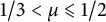
Finally, we verify in various cases. Keep in mind that $\varPi = T^{\mu }$ and ${P = T^{v}}$ . For $1/2 < \mu < 1$ , and this is $o (\varPi T)$ as long as ${v < 1 + \mu }$ . For $1/3 < \mu \leqslant 1/ 2$ , and this is satisfactory for $v < 3 \mu $ . For $0 < \mu \leqslant 1/3$ , is negligible for $v < 1$ as the c-sum is void (of course, in this case, (15.7) also follows from (15.5) in Lemma 15.1). Moreover, in view of Remark 13.1, one may treat the other in a similar or easier manner.

16 Proof of the non-vanishing results on the Riemann hypothesis

Let us modify the argument in [Reference Iwaniec, Luo and SarnakILS] as follows. Put

(16.1)

where the $\delta $ in the sum is the Kronecker $\delta $ -symbol (not to be confused with the parity $\delta $ in ). Clearly,

(16.2) $$ \begin{align} \sum_{m=0}^{\infty} p^{\delta}_{m} (T, \varPi) = 1. \end{align} $$ sigma summation Underscript m equals 0 Overscript infinity Endscripts p Subscript m Superscript delta Baseline left parenthesis upper T comma upper Pi right parenthesis equals 1 period

On the other hand, we choose, as in [Reference Iwaniec, Luo and SarnakILS, Formula (1.42)], the Fourier pair

(16.3) $$ \begin{align} \unicode{x3c6} (x) = \bigg(\frac {\sin (\pi v x)} {\pi v x} \bigg)^2 , \quad \hat{\unicode{x3c6}} (y) = \frac 1 {v} \bigg(1 - \frac {|y|} {v} \bigg), \qquad \text{(|y| < v)}, \end{align} $$

for every $v < v (\mu )$ (see (15.6)). By the definition in (1.19), it follows from $ \unicode{x3D5} (0) = 1 $ and the non-negativity of $\unicode{x3c6} $ that

$$ \begin{align*} D (f; \unicode{x3c6}; T) \geqslant \mathop{\mathrm{ord}}_{ s = s_f} L (s, f). \end{align*} $$

Also note that

$$ \begin{align*}\hat{\unicode{x3c6}} (0) = \frac 1 {v} .\end{align*} $$

Thus, for $ 1/3 < \mu < 1$ , we derive from (1.20), (1.22), and (1.23) that

(16.4) $$ \begin{align} \sum_{m=1}^{\infty} m p^{\delta}_{m} (T, \varPi) < \frac 1 {v (\mu)} + \varepsilon , \qquad \varPi = T^{\mu}, \end{align} $$ sigma summation Underscript m equals 1 Overscript infinity Endscripts m p Subscript m Superscript delta Baseline left parenthesis upper T comma upper Pi right parenthesis less than StartFraction 1 Over v left parenthesis mu right parenthesis EndFraction plus epsilon comma upper Pi equals upper T Superscript mu Baseline comma

for any $\varepsilon> 0$ , provided that T is sufficiently large. By subtracting (16.4) from (16.2), we obtain the lower bound

(16.5) $$ \begin{align} p^{\delta}_{0} (T, T^{\mu})> 1 - \frac 1 {v (\mu)} -\varepsilon. \end{align} $$

Note that (16.5) is non-trivial only if $ v (\mu )> 1 $ ; so, we do need $ 1/3 < \mu < 1$ as above. In view of (15.6) and (16.1), let us reinterpret (16.5) as

(16.6)

Similar to the argument in Section 10.4, we may remove the smooth and harmonic weights by Lemma 5.1 and the technique of Kowalski and Michel [Reference Kowalski and MichelKM1]. Consequently, we arrive at (1.6) and (1.7) in Theorems 3 and 4.

A Addendum: Non-vanishing of central L-values on the Riemann hypothesis

In this addendum, we take the opportunity to improve Theorem A.3 in [Reference Liu and QiLQ1] as follows, with the restriction $\mu> 1/3$ removed, and also to establish conditional non-vanishing results by (1.40)–(1.45) in [Reference Iwaniec, Luo and SarnakILS] for the central L-values $L (1/2 , f)$ or $L' (1/2, f)$ in the even or odd case.

Theorem A.1 Let the notation be as in the Appendix in [Reference Liu and QiLQ1]. Assume the Riemann hypothesis for Dirichlet L-functions. Let $ T, M> 1$ be such that $M = T^{\mu }$ with $0 < \mu < 1$ . Define

(A.1) $$ \begin{align} v (\mu) = \left\{ \begin{aligned} & 1, & & \text{ if }\ 0 < \mu \leqslant 1/4,\\ & 4 \mu, & & \text{ if }\ 1/4 < \mu \leqslant 1/3, \\ & 1 + \mu, & & \text{ if }\ 1/3 < \mu < 1. \end{aligned}\right. \end{align} $$

Let $\unicode{x3c6} $ be an even Schwartz function with the support of $\hat {\unicode{x3c6} }$ in $(-v (\mu ), v (\mu ) )$ . Then,

(A.2)

(A.3)

Proof It only requires minor modifications to the proof of Theorem A.3 (indeed, Lemmas A.8 and A.9 in [Reference Liu and QiLQ1]).

As in (A.21) and (A.23) in [Reference Liu and QiLQ1], we need to analyze integrals of the form:

$$ \begin{align*} H_{T, M}^{- \sharp} (x) &= \frac {2 M T } {\pi^2} \int_{-M^{\varepsilon }/M}^{M^{\varepsilon }/ M} \widehat{k} (-Mr/\pi) e ( T r / \pi) \cos ( 4 \pi x \sinh r ) \mathrm{d} r,\\H_{T, M}^{- \natural} (x) &= - \frac {8 M T } {\pi} \int_{-M^{\varepsilon }/M}^{M^{\varepsilon }/ M} \widehat{k} (-Mr/\pi) \sinh r \cdot e ( T r / \pi) \sin ( 4 \pi x \sinh r ) \mathrm{d} r, \end{align*} $$

StartLayout 1st Row 1st Column upper H Subscript upper T comma upper M Superscript negative normal sharp Baseline left parenthesis x right parenthesis 2nd Column equals StartFraction 2 upper M upper T Over pi squared EndFraction integral Subscript minus upper M Superscript epsilon Baseline divided by upper M Superscript upper M Superscript epsilon Baseline divided by upper M Baseline ModifyingAbove k With caret left parenthesis minus upper M r divided by pi right parenthesis e left parenthesis upper T r divided by pi right parenthesis cosine left parenthesis 4 pi x hyperbolic sine r right parenthesis normal d r comma 2nd Row 1st Column upper H Subscript upper T comma upper M Superscript negative normal natural Baseline left parenthesis x right parenthesis 2nd Column equals minus StartFraction 8 upper M upper T Over pi EndFraction integral Subscript minus upper M Superscript epsilon Baseline divided by upper M Superscript upper M Superscript epsilon Baseline divided by upper M Baseline ModifyingAbove k With caret left parenthesis minus upper M r divided by pi right parenthesis hyperbolic sine r dot e left parenthesis upper T r divided by pi right parenthesis sine left parenthesis 4 pi x hyperbolic sine r right parenthesis normal d r comma EndLayout

where $ \widehat {k} (- r/\pi ) $ is a Schwartz function similar to the $g ( r )$ as in Lemma 4.2. As in the second statement of Lemma A.8 in [Reference Liu and QiLQ1], under the condition $ \mu> 1 / 3 $ , it is proven that $H_{T, M}^{- \sharp } (x) $ and $ H_{T, M}^{- \natural } (x) $ are negligibly small unless $ |T-2\pi x| \leqslant M^{1+\varepsilon } $ . The reader should compare these integrals with those in (13.2) and (13.5). Note that the derivatives of the phase functions here satisfy

$$ \begin{align*} T / \pi - 2 x \cosh r = T /\pi - 2 x + O (xM^{\varepsilon } / M^2), \qquad T / \pi + 2 x \cosh r> T/\pi. \end{align*} $$

For this theorem, it suffices to remove the condition $\mu> 1/3$ but weaken the range $ |T-2\pi x| \leqslant M^{1+\varepsilon } $ into $ |T-2\pi x| \leqslant M^{\varepsilon } (M + T/M^2) $ . To this end, we may apply Lemma B.1 in [Reference QiQi] with $S = 1$ , $ P = 1/ M $ , $Q = M^{\varepsilon } / M$ , $Z = T / M^3 $ , and $ R = M^{\varepsilon } ( M +T / M^2 ) $ . This is essentially in the spirit of our Lemma 13.1. Now, for $P = T^{2v}$ , it is easy to verify that the error bound $O (\sqrt {P} T^{\varepsilon })$ becomes $ O (\sqrt {P} (1+T/M^3) T^{\varepsilon }) $ (for ; otherwise, the c-sum is void) in the first part of the proof of Lemma A.9 in [Reference Liu and QiLQ1].

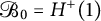
Note that in the notation of this article, , , and $\varPi = M$ .

Next, we assume the Riemann hypothesis for every $L (s, f)$ with $ f \in H^{\pm } (1) $ and for all Dirichlet L-functions. The following results may be derived from Theorem A.1 by adapting the arguments from Sections 10.4 and 16 and also [Reference Iwaniec, Luo and SarnakILS]. The reader may compare Corollary A.1 with Corollary 1.7 in [Reference Iwaniec, Luo and SarnakILS].

Corollary A.1 We have

(A.4) $$ \begin{align} \liminf_{T \rightarrow \infty} \frac {\mathrm{\boldsymbol \#} \big\{ f \in H^{+} (1) : t_f \leqslant T , \, L (1/2 , f ) \neq 0 \big\}} {\mathrm{\boldsymbol \#} \big\{ f \in H^{+} (1) : t_f \leqslant T \big\} }> \frac 9 {16} , \end{align} $$

(A.5) $$ \begin{align} \liminf_{T \rightarrow \infty} \frac {\mathrm{\boldsymbol \#} \big\{ f \in H^{-} (1) : t_f \leqslant T , \, L ' (1/2 , f ) \neq 0 \big\}} {\mathrm{\boldsymbol \#} \big\{ f \in H^{-} (1) : t_f \leqslant T \big\} }> \frac {15} {16}. \end{align} $$

Corollary A.2 We have

(A.6) $$ \begin{align} \liminf_{T \rightarrow \infty} \frac {\mathrm{\boldsymbol \#} \big\{ f \in H^{+} (1) : |t_f - T| \leqslant T^{\mu} , \, L (1/2 , f ) \neq 0 \big\}} {\mathrm{\boldsymbol \#} \big\{ f \in H^{+} (1) : |t_f - T| \leqslant T^{\mu} \big\} } \geqslant \frac 1 {4} , \end{align} $$

(A.7) $$ \begin{align} \liminf_{T \rightarrow \infty} \frac {\mathrm{\boldsymbol \#} \big\{ f \in H^{-} (1) : |t_f - T| \leqslant T^{\mu} , \, L ' (1/2 , f ) \neq 0 \big\}} {\mathrm{\boldsymbol \#} \big\{ f \in H^{-} (1) : |t_f - T| \leqslant T^{\mu} \big\} } \geqslant \frac {3} {4} , \end{align} $$

if $ 0 < \mu \leqslant 1/4$ , and

(A.8) $$ \begin{align} & \liminf_{T \rightarrow \infty} \frac {\mathrm{\boldsymbol \#} \big\{ f \in H^{+} (1) : |t_f - T| \leqslant T^{\mu} , \, L (1/2 , f ) \neq 0 \big\}} {\mathrm{\boldsymbol \#} \big\{ f \in H^{+} (1) : |t_f - T| \leqslant T^{\mu} \big\} }> 1 - \frac 1 {v (\mu )} + \frac 1 {4 v (\mu )^2} , \end{align} $$

(A.9) $$ \begin{align} & \quad \liminf_{T \rightarrow \infty} \frac {\mathrm{\boldsymbol \#} \big\{ f \in H^{-} (1) : |t_f - T| \leqslant T^{\mu} , \, L ' (1/2 , f ) \neq 0 \big\}} {\mathrm{\boldsymbol \#} \big\{ f \in H^{-} (1) : |t_f - T| \leqslant T^{\mu} \big\} }> 1 - \frac 1 {4 v (\mu )^2} , \end{align} $$

if $1/4 < \mu < 1$ , for

(A.10) $$ \begin{align} v (\mu ) = \min \{ 4\mu, 1+\mu \}. \end{align} $$

Acknowledgments

The author gratefully acknowledges the referees for identifying several errors in the manuscript and offering numerous valuable suggestions that substantially improved the exposition.

Footnotes

The author was supported by the National Key R&D Program of China (Grant No. 2022YFA1005300).

References

Alpoge, L. and Miller, S. J., Low-lying zeros of Maass form $L$

-functions . Int. Math. Res. Not. IMRN 10(2015), 2678–2701.Google Scholar

Balkanova, O., Huang, B., and Södergren, A., Non-vanishing of Maass form $L$

-functions at the central point . Proc. Amer. Math. Soc. 149(2021), no. 2, 509–523.10.1090/proc/15208CrossRef Google Scholar

Blomer, V., Subconvexity for twisted $L$

-functions on $\mathrm{GL}(3)$

. Amer. J. Math. 134(2012), no. 5, 1385–1421.10.1353/ajm.2012.0032CrossRef Google Scholar

Bohr, H. and Landau, E., Sur les zéros de la fonction $\zeta (s)$

de Riemann . C. R. Acad. Sci. Paris 158(1914), 106–110.Google Scholar

Bourgain, J. and Watt, N., Decoupling for perturbed cones and the mean square of $|\zeta (\frac{1}{2} + \textit{it})|$

. Int. Math. Res. Not. IMRN 17(2018), no. 17, 5219–5296.10.1093/imrn/rnx009CrossRef Google Scholar

Conrey, J. B. and Iwaniec, H., The cubic moment of central values of automorphic $L$

-functions . Ann. of Math. (2) 151(2000), no. 3, 1175–1216.10.2307/121132CrossRef Google Scholar

Deshouillers, J.-M. and Iwaniec, H., The nonvanishing of Rankin-Selberg zeta-functions at special points . In: D. A. Hejhal, P. Sarnak, and A. A. Terras (eds.), The Selberg trace formula and related topics (Brunswick, Maine, 1984), Contemporary Mathematics, 53, American Mathematical Society, Providence, RI, 1986, pp. 51–95.10.1090/conm/053/853553CrossRef Google Scholar

Ivić, A. and Jutila, M., On the moments of Hecke series at central points. II . Funct. Approx. Comment. Math. 31(2003), 93–108.10.7169/facm/1538186641CrossRef Google Scholar

Iwaniec, H. and Kowalski, E., Analytic number theory, American Mathematical Society Colloquium Publications, 53, American Mathematical Society, Providence, RI, 2004.10.1090/coll/053CrossRef Google Scholar

Iwaniec, H. and Li, X., The orthogonality of Hecke eigenvalues . Compos. Math. 143(2007), no. 3, 541–565.10.1112/S0010437X07002679CrossRef Google Scholar

Iwaniec, H., Luo, W., and Sarnak, P., Low lying zeros of families of $L$

-functions . Inst. Hautes Études Sci. Publ. Math. 91(2000), 55–131.10.1007/BF02698741CrossRef Google Scholar

Iwaniec, H. and Sarnak, P., The non-vanishing of central values of automorphic $L$

-functions and Landau-Siegel zeros . Israel J. Math. 120(2000), 155–177. (Part A).10.1007/s11856-000-1275-9CrossRef Google Scholar

Katz, N. M. and Sarnak, P., Random matrices, Frobenius eigenvalues, and Monodromy, American Mathematical Society Colloquium Publications, 45, American Mathematical Society, Providence, RI, 1999.Google Scholar

Kim, H. H., Functoriality for the exterior square of $\mathrm{GL}_4$

and the symmetric fourth of $\mathrm{GL}_2$

. J. Amer. Math. Soc. 16(2003), no. 1, 139–183. With appendix 1 by Dinakar Ramakrishnan and appendix 2 by Kim and Peter Sarnak.10.1090/S0894-0347-02-00410-1CrossRef Google Scholar

Kowalski, E. and Michel, P., The analytic rank of ${J}_0(q)$

and zeros of automorphic $L$

-functions . Duke Math. J. 100(1999), no. 3, 503–542.10.1215/S0012-7094-99-10017-2CrossRef Google Scholar

Kowalski, E. and Michel, P., A lower bound for the rank of ${J}_0(q)$

. Acta Arith. 94(2000), no. 4, 303–343.10.4064/aa-94-4-303-343CrossRef Google Scholar

Li, X., Bounds for $\mathrm{GL}(3) \times \mathrm{GL}(2)\ L$

-functions and $\mathrm{GL}(3)\ L$

-functions . Ann. of Math. (2) 173(2011), no. 1, 301–336.10.4007/annals.2011.173.1.8CrossRef Google Scholar

Li, X., A weighted Weyl law for the modular surface . Int. J. Number Theory 7(2011), no. 1, 241–248.10.1142/S1793042111003995CrossRef Google Scholar

Liu, S.-C. and Qi, Z., Low-lying zeros of $L$

-functions for Maass forms over imaginary quadratic fields . Mathematika 66(2020), no. 3, 777–805.10.1112/mtk.12041CrossRef Google Scholar

Liu, S.-C. and Qi, Z., Moments of central $L$

-values for Maass forms over imaginary quadratic fields . Trans. Amer. Math. Soc. 375(2022), no. 5, 3381–3410.Google Scholar

Luo, W., On the nonvanishing of Rankin-Selberg $L$

-functions . Duke Math. J. 69(1993), no. 2, 411–425.10.1215/S0012-7094-93-06918-9CrossRef Google Scholar

Luo, W., The spectral mean value for linear forms in twisted coefficients of cusp forms . Acta Arith. 70(1995), no. 4, 377–391.10.4064/aa-70-4-377-391CrossRef Google Scholar

Luo, W., Nonvanishing of $L$

-values and the Weyl law . Ann. of Math. (2) 154(2001), no. 2, 477–502.10.2307/3062104CrossRef Google Scholar

Luo, W., Refined asymptotics for second spectral moment of Rankin-Selberg $L$

-functions at the special points . Int. Math. Res. Not. IMRN 23(2012), 5457–5483.10.1093/imrn/rnr243CrossRef Google Scholar

Magnus, W., Oberhettinger, F., and Soni, R. P., Formulas and theorems for the special functions of mathematical physics. 3rd enlarged ed., Die Grundlehren der mathematischen Wissenschaften, 52, Springer-Verlag New York, Inc., New York, NY, 1966.10.1007/978-3-662-11761-3CrossRef Google Scholar

Phillips, R. S. and Sarnak, P., On cusp forms for co-finite subgroups of $\mathrm{PSL}(2,\mathbf{R})$

. Invent. Math. 80(1985), no. 2, 339–364.10.1007/BF01388610CrossRef Google Scholar

Qi, Z., On the effective non-vanishing of Rankin–Selberg $L$

-functions at special points. Peking Math. J. (accepted).Google Scholar

Rudnick, Z. and Sarnak, P., Zeros of principal $L$

-functions and random matrix theory . Duke Math. J. 81(1996), no. 2, 269–322.10.1215/S0012-7094-96-08115-6CrossRef Google Scholar

Selberg, A., On the zeros of Riemann’s zeta-function . In: Collected papers. Vol. I, Springer-Verlag, Berlin, 1989, pp. 85–141.Google Scholar

Titchmarsh, E. C., The theory of the Riemann zeta-function. 2nd ed., The Clarendon Press, Oxford University Press, New York, NY, 1986. Edited and with a preface by D. R. Heath-Brown.Google Scholar

Watson, G. N., A treatise on the theory of Bessel functions, Cambridge University Press, The Macmillan Company, Cambridge, New York, NY, 1944.Google Scholar

Xu, Z., Nonvanishing of automorphic $L$

-functions at special points . Acta Arith. 162(2014), no. 4, 309–335.10.4064/aa162-4-1CrossRef Google Scholar

Young, M. P., Weyl-type hybrid subconvexity bounds for twisted $L$

-functions and Heegner points on shrinking sets . J. Eur. Math. Soc. (JEMS) 19(2017), no. 5, 1545–1576.10.4171/jems/699CrossRef Google Scholar

Figure 1: A comparison of the proportions in (1.5) and (1.7).Figure 1. long description.

Article contents

On the effective non-vanishing of Hecke–Maass L-functions at special points

Abstract

Keywords

MSC classification

Information

1 Introduction

1.1 Definitions

1.2 Effective non-vanishing results

Theorem [Reference QiQi]

1.3 Twisted spectral moments

1.4 Density theorems

Notation

2 Kuznetsov trace formulas

2.1 The Kloosterman sum

2.2 The Hecke relation

2.3 The Weyl law

3 Hecke–Maass L-functions

4 Analysis for the Bessel integrals

5 A useful unsmoothing lemma

6 Preliminaries

6.1 Poisson summation formula

6.2 Mean-value bounds for the Riemann $\zeta $ function

6.3 Approximate functional equations

6.4 Bi-variable notation

7 Setup

8 The twisted first moment

8.1 Application of the Kuznetsov formula

8.2 Asymptotic for the diagonal term

8.3 Estimation of the off-diagonal sums

8.4 Conclusion

9 The twisted second moment

9.1 Application of the Kuznetsov formula

9.2 Asymptotic for the diagonal sum

9.3 Estimation of the off-diagonal sums

9.4 Conclusion

10 The mollified moments

10.1 Setup

10.2 The mollified first moment

10.3 The mollified second moment

10.4 Conclusion

11 Moments with no twist and smooth weight

12 Sums of variant Kloosterman sums

13 Further analysis for the Bessel integrals

14 The explicit formula

15 Proof of the density theorems

Notation

15.1 Application of the Kuznetsov formula

15.2 Proof of Lemma 15.1

15.3 Proof of Lemma 15.2

16 Proof of the non-vanishing results on the Riemann hypothesis

A Addendum: Non-vanishing of central L-values on the Riemann hypothesis

Acknowledgments

Footnotes

References

Save article to Kindle

Save article to Dropbox

Save article to Google Drive

Reply to: Submit a response

Your details

You have entered the maximum number of contributors

Conflicting interests