1. Introduction and results
In this article we deal with conservative maps on the two-torus
 $\mathbb {T}^2$
, that is, maps preserving the Lebesgue (Haar) measure
 $\mu$
. In smooth ergodic theory one is typically interested in the asymptotic behavior exhibited by the system under consideration, and a basic (but nonetheless powerful) mechanism for the analysis is provided by the Lyapunov exponents. For completeness we will recall the definition below, but we assume some familiarity of the reader with these concepts, as covered for example in [Reference Barreira and PesinBP13]. We will, however, focus on the two-dimensional case and discuss this setting only.
Definition 1.1. For a differentiable map
 $f:\mathbb {T}^2\to \mathbb {T}^2$
and a vector
 $(x,v)\in T\mathbb {T}^2$
with
 $v\neq 0$
, the quantity
 \begin{align*} \bar {\chi }(x,v)=\limsup _{n\to \infty }\frac {\log \left \Vert D_xf^n(v)\right \Vert }{n} \end{align*}
is the Lyapunov exponent of
 $f$
at
 $(x,v)$
.
Classical results (see, for example, [Reference Furstenberg and KestenFK60]) show that one can find a full area set
 $M'$
such that for points
 $x\in M'$
the previous limit exists (we denote it by
 $\chi (x,v)$
) for every
 $v\neq 0$
and coincides with one of the following two quantitiesFootnote
1
:
 \begin{align*} \chi ^+(x)&=\lim _{n\to +\infty }\frac {\log \left \Vert D_xf^n\right \Vert }{n},\\ \chi ^-(x)&=\lim _{n\to +\infty }\frac {\log \mathrm {m}\left (D_xf^n\right )}{n}. \end{align*}
In fact, as a result of Oseledets’ theorem [Reference OseledetsOse68] there exists a measurable bundle
 $E^-$
defined on a full measure set
 $M_0$
such that for
 $x\in M_0, 0\neq v\in E^{-}(x)\Rightarrow \chi (x,v)=\chi ^{-}(x), v\in {\mathbb {R}^2}\setminus E^{-}(x)\Rightarrow \chi (x,v)=\chi ^{+}(x)$
. One can check that
 \begin{equation*} \int (\chi ^{+}(x)+\chi ^{-}(x))\, d\mu (p)=\int \log |\!\det D_xf|\, d\mu (x)\gt 0, \end{equation*}
so
 $\chi ^{+}(x)\gt 0$
almost everywhere.
Definition 1.2. The map
 $f$
is non-uniformly hyperbolic (NUH) if
 $\chi ^-\lt 0\lt \chi ^+$
 $\mu$
-almost everywhere.
Non-uniform hyperbolicity means that there is exponential divergence of orbits, both in the past and in the future. This notion, introduced by Y. Pesin, generalizes classical hyperbolicity, and it is difficult to overemphasize its importance in modern dynamics.
A basic feature of NUH diffeomorphisms is that, even though they can be found on any surface [Reference KatokKat79] (and indeed, on any closed manifold of dimension larger than one [Reference Dolgopyat and PesinDP02]), they are typically fragile in the following sense: any conservative surface diffeomorphism
 $f$
can be approximated in the
 $\mathcal {C}^1$
topology by a diffeomorphism having zero exponents, unless
 $f$
is Anosov. This is a consequence of the Bochi–Mañé theorem [Reference BochiBoc02], and reveals a rigidity phenomena for such systems.
It is remarkable that the corresponding question for endomorphisms has not been addressed before, but this can be explained by the surplus of additional difficulties presented by the non-invertible case, leading to a much less developed theory than for the corresponding invertible counterpart. The aim of this paper is to make a contribution to the ergodic theory of non-invertible endomorphisms of
 $\mathbb {T}^2$
, and present interesting new phenomena that will perhaps motivate additional research.
In contrast to the case of diffeomorphisms, we will establish the existence of
 $\mathcal C^1$
robust NUH endomorphisms in
 $\mathbb {T}^2$
, without essentially any topological obstruction. These examples share several similarities with hyperbolic diffeomorphisms. On the one hand, their integrated Lyapunov exponents (and therefore their exponents in the ergodic case) depend continuously on the map. We point out to the reader that, as a consequence of the Bochi–Mañé theorem cited above, this is not true for diffeomorphisms except for Anosov ones. On the other hand, assuming transitivity of their linear part (which can easily be checked by looking at the eigenvalues of the associated matrix), they are ergodic (and even Bernoulli, see § 1.3), and they remain so under
 $\mathcal C^2$
perturbations. Therefore, the class of systems introduced in this article seems to have enough robustness to permit a thorough analysis, and we hope to motivate the reader to explore this new realm.
1.1 Existence of robust NUH endomorphisms
Any map
 $f:\mathbb {T}^2\to \mathbb {T}^2$
is homotopic to a linear endomorphism
 $E$
induced by an integer matrix that we denote by the same letter. In this work, we are interested in non-invertible local diffeomorphisms and will therefore only consider the case when
 $|\!\det E | \geq 2$
. Considering the projective action
 ${\mathbb {P}} E: {\mathbb {P}} {\mathbb {R}^2} \to {\mathbb {P}} {\mathbb {R}^2}$
that induces
 $E$
, we have four possibilities:
-
–
 ${\mathbb {P}} E=\mathrm {Id}$
;
-
– there exists a parabolic fix point
$p\in {\mathbb {P}} {\mathbb {R}^2}$
that is repelling on one side and attracting on the other; -
– there exist two hyperbolic fix points
$p,q\in {\mathbb {P}} {\mathbb {R}^2}$
, and the dynamics is of the north pole–south pole type; or -
–
${\mathbb {P}} E$
is conjugated to a rotation.


Note that the first corresponds to the case when
 $E$
is a homothety.
If
 $f:\mathbb {T}^2\to \mathbb {T}^2$
is of class
 $\mathcal C^1$
we consider the class of
 $\mathcal C^1$
smoothly homotopic maps to
 $f$
,
 \begin{equation*} [f]=\{g:\mathbb {T}^2\to \mathbb {T}^2: \text {there exists a }\mathcal C^1\text { homotopy between $f$ and $g$}\}. \end{equation*}
We denote by
 $\mathrm {End}_{\mu }^r(\mathbb {T}^2)$
the set of
 $\mathcal C^r$
local diffeomorphisms of
 $\mathbb {T}^2$
preserving the Lebesgue measure
 $\mu$
that are not invertible. For
 $f\in \mathrm {End}^1_{\mu }(\mathbb {T}^2), (x,v)\in T^1\mathbb {T}^2$
we define
 \begin{equation} I(x,v;f^n)=\sum _{y\in f^{-n}(x)}\frac {\log \|(D_yf^n)^{-1}v\|}{|\!\det (D_yf^n)|}, \end{equation}
and let
 \begin{equation} C_{\chi }(f)=\sup _{n\in \mathbb N}\frac 1n\inf _{(x,v)\in T^1\mathbb {T}^2}I(x,v;f^n). \end{equation}
The set
 \begin{equation} \mathcal U:=\{f\in \mathrm {End}^1_{\mu }(\mathbb {T}^2):\ C_{\chi }(f)\gt 0\} \end{equation}
is open in the
 $\mathcal C^1$
topology: indeed, if
 $f\in \mathcal U$
then for some
 $n$
it follows that
 $(1/n)\inf _{(x,v)\in T^1\mathbb {T}^2}I(x,v;f^n)\gt {C_{\chi }(f)}/{2}$
, and hence taking a sufficiently small
 $\mathcal C^1$
neighborhood
 $\mathcal V$
of
 $f$
we can guarantee that any
 $g\in \mathcal V$
is an endomorphism and satisfies
 $(1/n)\inf _{(x,v)\in T^1\mathbb {T}^2}I(x,v;g^n)\gt {C_{\chi }(f)}/{4}$
, thus implying that
 $g\in \mathcal U$
.
Our first main result is the following.
Theorem A.
Any
 $f\in \mathcal U$
is non-uniformly hyperbolic. Moreover, if
 $E=(e_{ij})\in \mathrm {M}_{2 \times 2}(\mathbb {Z})$
is not a homothety and
 $|\!\det E|/\gcd {e_{ij}}\gt 4$
, then the intersection
 $[E]\cap \mathcal U$
is non-empty, and in fact contains maps that are real analytically homotopic to
 $E$
.
This, in particular, establishes the existence of
 $\mathcal C^1$
open sets of NUH endomorphisms. The above is a flexibility theorem: unlike the diffeomorphism case, there are no topological obstructions to the existence of robust NUH endomorphisms in
 $\mathbb {T}^2$
. We also point out that this is the first robustly NUH (area-preserving) example of an endomorphism, that it is not expanding, and that it does not admit an invariant distribution.
Remark 1.1. If
 $\tau _1(E)=\gcd {e_{ij}}, \tau _2(E)=|\!\det E|/\tau _1(E)$
, then the Smith Normal Form of
 $E$
is the diagonal matrix with entries
 $\tau _1(E)$
and
 $\tau _2(E)$
(see § 2.4). The condition on
 $\tau _2(E)$
from Theorem
A is valid for all pairs
 $(\tau _1(E),\tau _2(E))$
with the exception of those in
 \begin{equation*} \{(1,2), (1,3), (1,4), (2, 2), (2,4), (3,3), (4,4)\}. \end{equation*}
This requirement on
 $\tau _2(E)$
and the non-homothety assumption are made to avoid some technical difficulties, and we expect that with additional work this restriction can be lifted to any (non-invertible) endomorphism; see § 1.5. Let us also point out that our methods give effective bounds for the
 $\mathcal {C}^1$
distance between constructed elements
 $f\in [E]\cap \mathcal U$
and
 $E$
.
Observe the following curious consequence.
Corollary 1.1.
If
 $F:\mathbb {T}^2\to \mathbb {T}^2$
is a
 $\mathcal {C}^1$
uniformly expanding map of degree larger than
 $16$
that is not homotopic to a homothety, then it is a factor (semi-conjugate) of a smooth conservative map
 $f$
that is non-uniformly hyperbolic with one positive and one negative Lyapunov exponent.
Proof.
By [Reference ShubShu69]
 $F$
is conjugate to its linear part
 $E$
, and
 $E$
is a factor of the map
 $f$
constructed in Theorem A.
For any such expanding map, both its exponents are necessarily positive (in fact, this is the case with respect to any of its invariant measures). Nevertheless, it can be obtained as a quotient of a system which has contracting direction at Lebesgue almost every point of its phase space.
1.2 Continuity of the exponents
A natural question which arises is how the Lyapunov exponents depend on the map
 $f$
. Since we do not know a priori that
 $f$
is ergodic, it makes sense to ask about the regularity of the maps
 $f\mapsto \int _{\mathbb {T}^2}\chi ^-(f)\,d\mu$
,
 $f\mapsto \int _{\mathbb {T}^2}\chi ^+(f)\,d\mu$
, for
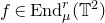 $f\in \mathrm {End}^r_{\mu }(\mathbb {T}^2)$
,
 $r\geq 1$
.
The classical results of Mañe, Bochi and Viana show that one cannot expect continuity in the
 $\mathcal C^1$
topology for diffeomorphisms without dominated (Oseledets) splitting. Continuity in finer topologies is known for certain restricted classes of diffeomorphism, but the general panorama is still not clear. The reader is referred to [Reference Liang, Marin and YangLMY18] and references therein for a discussion in the diffeomorphism (partially hyperbolic) setting. For continuity of Lyapunov exponents for cocycles over homeomorphisms, the reader can check the survey in [Reference VianaVia18].
On the other hand, the results in [Reference Viana and YangVY19] for cocycles over endomorphisms suggest that we may be able to obtain better regularity than in the invertible counterpart. Indeed, we obtain the following result.
Define
 \begin{equation*} C_{\det }(f)=\sup _{n\in \mathbb N}\frac 1n\inf _{x\in M}\log |\!\det (Df_x^n)|\gt 0 \end{equation*}
and
 \begin{equation} \mathcal U_1=\left \{ f\in \mathrm {End}^1_{\mu }(\mathbb {T}^2): C_{\chi }(f)\gt -\tfrac 12C_{\det }(f)\right \}, \end{equation}
where
 $C_{\chi }(f)$
is defined in (2). Clearly
 $\mathcal U_1$
is open and contains the set
 $\mathcal U$
of NUH endomorphisms constructed in Theorem A.
Theorem B.
The maps
 $\mathcal U_1\ni f\mapsto \int _{\mathbb {T}^2}\chi ^-(f)\,d\mu$
,
 $\mathcal U_1\ni f\mapsto \int _{\mathbb {T}^2}\chi ^+(f)\,d\mu$
are continuous in the
 $\mathcal C^1$
topology.
An immediate consequence of the Pesin formula for endomorphisms [Reference Qian and ZhuQZ02] is the result below.
Corollary 1.2.
The map
 $\mathcal U\ni f\mapsto h_{\mu }(f)$
is continuous in the
 $\mathcal C^1$
topology. Here
 $h_{\mu }(f)$
denotes the metric entropy of
 $f$
with respect to
 $\mu$
.
1.3 Stable ergodicity
Some of the examples constructed can be shown to be stably ergodic.
Definition 1.3. We say that an endomorphism
 $f$
is stably ergodic (for
 $\mu$
) if there exists a
 $\mathcal C^1$
neighborhood
 $\mathcal U'$
of
 $f$
in
 $\mathrm {End}^1_{\mu }(\mathbb {T}^2)$
such that every
 $g\in \mathcal {U'}$
of class
 $\mathcal {C}^{2}$
is also ergodic.
The study of stably ergodic diffeomorphisms (that are not uniformly hyperbolic) was initiated by the results of Grayson, Pugh and Shub [Reference Grayson, Pugh and ShubGPS94], and was promoted by Pugh and Shub to a theory which is currently attracting a large amount of research. Citing all this literature would lead us astray, so we will content ourselves by indicating some significant recent articles and referring the reader to them for additional information: [Reference Burns and WilkinsonBW10, Reference Hertz, Hertz and UresHHU08, Reference Avila, Crovisier and WilkinsonACW21].
Despite its popularity in the context of invertible dynamics, stable ergodicity for endomorphisms has never been given serious attention. In fact, we are unaware of any earlier attempt to give examples outside the realm of uniformly expanding systems. On the other hand, there are quite a few studies of physical measures for endomorphisms, and some of these can be translated into results about stable ergodicity. Most notably, for maps that are non-uniformly expanding in the sense of [Reference Alves, Bonatti and VianaABV00], the basins of physical measures are open. In a conservative context, this translates into the statement that ergodic components of Lebesgue measure are open (modulo sets of zero Lebesgue measure). Therefore, robust almost everywhere non-uniform expansion, together with robust transitivity, implies stable ergodicity.
For partially hyperbolic endomorphisms we have a very complete picture in the dissipative setting thanks to the seminal work of Tsujii [Reference TsujiiTsu05]:
 $\mathcal C^2$
-generic partially hyperbolic local diffeomorphisms on
 $\mathbb {T}^2$
have a finite number of physical measures whose basins cover a set of full Lebesgue measure of the manifold. One of the curious facts is that these measures are absolutely continuous with respect to Lebesgue, even if the central Lyapunov exponent is slightly negative. In their recent paper [Reference Tsujii and ZhangTZ24] Tsujii and Zhang construct smooth families of endomorphisms that are non-uniformly hyperbolic with respect to the physical measure. These works seem to require regularity higher than
 $\mathcal C^2$
. In the conservative setting it is likely that one can generalize the concept of accessibility to partially hyperbolic endomorphisms (by looking at the inverse limit and considering
 $\pi _{\mathrm {ext}}(x)$
as the strong stable manifold of
 $x$
) and then adapt the Grayson–Pugh–Shub program to obtain stable ergodicity.
For partially hyperbolic endomorphisms having only admissible measures (the analog of Gibbs
 $u$
-states for non-invertible maps) and negative central Lyapunov exponents, the first author proved in [Reference AnderssonAnd10] that having a single physical measure is a
 $\mathcal C^2$
open property. For conservative maps, this translates into the statement that ergodicity implies (
 $\mathcal C^2$
) stable ergodicity. We find it very likely that such maps are indeed
 $\mathcal C^1$
stably ergodic, meaning that the map is ergodic and that every
 $\mathcal C^2$
map
 $\mathcal C^1$
close to it is also ergodic. This was proved by Yang [Reference YangYan21] in the analogous setting for diffeomorphisms, and we see no reason why his proof should not work for endomorphisms as well.
In this work we produce examples of stably ergodic endomorphisms of a rather exotic kind: robustly non-uniformly ergodic maps without any dominated splitting. This stands in sharp contrast to the invertible case. Indeed, it was shown by Bochi, Fayad and Pujals [Reference Bochi, Fayad and PujalsBFP06] that any stably ergodic diffeomorphism can be approximated by one having a dominated splitting.
Our contribution to the theory is the following.
Theorem C.
For any linear endomorphism
 $E$
as in Theorem
A
, if
 $\pm 1$
is not an eigenvalue of
 $E$
then
 $[E]\cap \mathcal U$
contains stably ergodic endomorphisms.
In fact,
 $[E]\cap \mathcal U$
consists of stably Bernoulli
Footnote
2
endomorphisms (and, in particular, maps that are mixing of all orders).
Thus, we obtain examples of stably ergodic non-uniformly hyperbolic endomorphisms that do not admit any invariant distribution, and therefore are not partially hyperbolic.
Theorem C above will be obtained as a consequence of the following general result, which is of independent interest. For the discussion of global stable manifolds and Pesin theory see § 5.
Theorem D.
Let
 $f$
be a
 $\mathcal C^2$
transitive area-preserving non-uniformly hyperbolic endomorphism on a surface. Suppose there exists
 $\lambda \gt 0$
such that for, almost every point, the diameter
Footnote
3
of the global stable manifold of
 $x$
is larger than
 $\lambda$
. Then
 $f$
is ergodic.
If, furthermore,
 $f^n$
is transitive for any positive natural number
 $n$
, then
 $f$
is Bernoulli.
1.4 Comments on the proofs
We will make some comments on the ideas of the proofs involved in this article.
A fundamental tool is the natural extension of the endomorphism
 $f$
: this is the space
 $\mathbf {L}_{f}$
of the backward orbits, with a natural projection
 $\pi _{\mathrm{ext}}$
to the torus. The endomorphism
 $f$
lifts to an invertible map
 $\hat {f}$
and the area
 $\mu$
lifts to an invariant measure
 $\hat {\mu }$
. The Lyapunov exponents of
 $f$
coincide with the Lyapunov exponents of the
 $Df$
cocycle lifted to
 $\mathbf {L}_{f}$
. An important observation is that
 $\lim _{n\rightarrow \infty } ({1}/{n})I(x,v;f^n)$
is exactly the integral of the Lyapunov exponents of the lifted cocycle at
 $(\hat {x},v)$
on the fiber
 $\pi _{\mathrm{ext}}^{-1}(x)$
with respect to the disintegration of
 $\hat {\mu }$
on
 $\pi _{\mathrm{ext}}^{-1}(x)$
. This will ultimately imply that any map in
 $\mathcal U$
must be non-uniformly hyperbolic.
Let us mention that the property defining
 $\mathcal U$
has a similar counterpart in the setting of random maps, namely the ‘uniform expansion property’ of Dolgopyat and Krikorian [Reference Dolgopyat and KrikorianDK07]. This property has several nice consequences for the properties of stationary measures, and was investigated in a series of papers including [Reference Dolgopyat and KrikorianDK07, Reference Brown and Rodriguez HertzBRH17, Reference ChungChu20, Reference LiuLiu16].
The basic ideas in the construction of the specific examples in the homotopy class of
 $E$
are the following. We modify
 $E$
such that we make the map (strongly) hyperbolic in some ‘good’ region
 $\mathcal G$
, which is chosen to be large enough that most of the backward orbits spend a substantial time inside it. In general, without some further control this may not be enough to obtain hyperbolicity, because even if one obtains a relatively good expansion on some large piece of orbit, it is possible that, once we loosen the control, the next entry in the good region is such that the expanding direction goes to the contracting direction, and thus all the hyperbolicity which we gained is lost. In order to avoid this we have to make some kind of non-degeneracy assumption; in particular, we construct the map with slightly different hyperbolicity in different parts of the good region
 $\mathcal G$
. Thus we may lose the hyperbolicity for some particular orbits, but we will maintain it for other ones, and this turns out to be enough to obtain the conclusion.
The proof of the continuity of the exponents is based on methods developed for the study of the Lyapunov exponents for cocycles with holonomies. The definition of
 $\mathcal U_1$
guarantees that the Lyapunov spectrum is simple at almost every point. We consider the projectivization of the cocycle over
 $\hat {f}$
, and the invariant measure
 $\hat {\mu }$
lifts to convex combinations of Dirac measures supported at the Oseledets subspaces at almost every point. Assume that a sequence
 $f_n$
converges to
 $f$
in the
 $\mathcal C^1$
topology. The only way the continuity of the exponents can fail is if a sequence of stable lifts of
 $\hat {\mu }$
for
 $f_n$
(lifts supported at the subspaces corresponding to the smallest Lyapunov exponent) does not converge to the stable lift of
 $\hat {\mu }$
for
 $f$
, or, in other words, the limit contains some parts of the unstable lift of
 $\hat {\mu }$
for
 $f$
. The stable lifts are invariant under the holonomy given by the projection
 $\pi _{\mathrm{ext}}$
, and this property can be passed to the limit. This would imply that there is a nontrivial part of the unstable lift of
 $\hat {\mu }$
for
 $f$
which is invariant under the
 $\pi _{\mathrm{ext}}$
holonomy. It turns out that this is impossible because of the definition of
 $\mathcal U_1$
, which already implies that the (strong) unstable Oseledets subspaces cannot be independent of the past, so they cannot be constant on
 $\pi _{\mathrm {ext}}$
fibers. This condition is reminiscent of the ‘non-random stable bundle’ case appearing in the classification theorem of Brown and Rodriguez Hertz [Reference Brown and Rodriguez HertzBRH17] of hyperbolic stationary measures for random diffeomorphisms of surfaces.
For the proof of the stable ergodicity we rely on the classical Hopf argument. In order to obtain the intersections between the stable and the unstable manifolds we introduce a new method: we first prove that the stable manifolds at almost every point have large diameter. This is different from the classical notion of ‘large Pesin manifolds’, because we do not have control on how the manifolds turn inside the torus. However, we can use ideas from Rodriguez Hertz, Rodriguez Hertz, Tahzibi and Ures [Reference Hertz, Hertz, Tahzibi and UresHHTU11] to show that in the case of endomorphisms on surfaces, large stable manifolds in our sense imply that the ergodic components are open modulo zero sets. In order to conclude the proof we use a result of Andersson [Reference AnderssonAnd16] on the transitivity of area-preserving endomorphisms on
 $\mathbb {T}^2$
.
1.5 Further questions
Here we make some comments and we ask some further questions related to this work.
-
(1) Non-uniformly hyperbolic endomorphisms in all homotopy classes: We proved that the
$\mathcal {C}^1$
open set
$\mathcal U$
of non-uniformly hyperbolic endomorphisms intersects most of the homotopy classes of endomorphisms.Question 1. Is it true that
$\mathcal U$
intersects all the homotopy classes of endomorphisms on
$\mathbb {T}^2$
?It is reasonable to expect that this is true. However, if the endomorphism
$E$
is a homothety then one has to construct a more complicated good hyperbolic region
$\mathcal G$
, and if the degree of
$E$
is very small then one should take into consideration the position of several pre-images of every point, in order that most of them fall into the good region. -
(2) Stable ergodicity in a more general setting: We can obtain the stable ergodicity of the non-uniformly hyperbolic endomorphisms under various restrictions. One of them is a restriction of the homotopy class (the eigenvalues must have absolute value different from one) in order to apply Andersson’s result on the transitivity of endomorphisms.
Question 2. Are there stably ergodic non-uniformly hyperbolic endomorphisms in every homotopy class of endomorphisms on
$\mathbb {T}^2$
?Another restriction comes from the proof of the existence of large stable manifolds: we need the good region to be large enough, with good hyperbolicity, and the critical region to be small. On the other hand, because of the area expansion, the unstable manifolds of a non-uniformly hyperbolic endomorphism are always large.
Question 3. Is it true that every transitive non-uniformly hyperbolic endomorphism on a surface is stably ergodic?
Our methods cannot be applied directly to large unstable manifolds, because they do not form a lamination, so one cannot immediately obtain intersections of stable and unstable manifolds. One does, however, obtain intersections between different unstable manifolds, and, with some further work, this may be enough to obtain the ergodicity. If the Jacobian of the endomorphism is constant, the proof of the ergodicity is straightforward from the absolute continuity of the
$\pi _{\mathrm{ext}}$
holonomy, so the difficult question is when the Jacobian is not constant. -
(3) More continuity of the exponents: In general the continuity of the exponents may fail if parts of the stable lift of the measure to the projectivization of the cocycle move in the limit to parts of the unstable lift. However, this would imply that the strong unstable subspaces are invariant under the
$\pi _{\mathrm{ext}}$
holonomy, and this seems to be a rigid situation.Question 4. Is it true that the average Lyapunov exponents are continuous in (an open dense subset of) the space of
$\mathcal C^1$
area-preserving endomorphisms of surfaces?One may also ask how the Lyapunov exponents depend on the invariant measure, not necessarily the Lebesgue measure.
Question 5. Can we say something about the continuity of the Lyapunov exponents of maps in
$\mathcal U_1$
with respect to the invariant measure, in a neighborhood of the Lebesgue measure? -
(4) Flexibility of Lyapunov exponents for endomorphisms on
$\mathbb {T}^2$
: Bochi, Katok and Rodriguez Hertz proposed in [Reference Bochi, Katok and HertzBKH22] a program regarding the flexibility of Lyapunov exponents for diffeomorphisms. The same questions can be addressed in the case of endomorphisms:Question 6 (Weak flexibility on
$\mathbb {T}^2$
). Given any two real numbers
$\lambda _1,\lambda _2$
with
$\lambda _1+\lambda _2\gt 0$
, does there exist an ergodic measure-preserving (smooth) endomorphism of
$\mathbb {T}^2$
with Lyapunov exponents
$\lambda _1$
and
$\lambda _2$
?Question 7 (Strong flexibility on
$\mathbb {T}^2$
). Given a linear endomorphism
$E$
of
$\mathbb {T}^2$
and
$\lambda _1,\lambda _2\in {\mathbb {R}^2}$
with
$0\lt \lambda _1+\lambda _2$
$\leq \log (|\!\det (E)|)$
, does there exist an ergodic measure-preserving (smooth) endomorphism of
$\mathbb {T}^2$
, isotopic to
$E$
, with Lyapunov exponents
$\lambda _1$
and
$\lambda _2$
?Our results answer the second question for many isotopy classes and for
$\lambda _1\ll 0\ll \lambda _2$
,
$\lambda _1+\lambda _2$
close to
$\log (|\!\det (E)|)$
. Any progress on Questions 1–5 above would also contribute to the flexibility program for endomorphisms on
$\mathbb {T}^2$
. -
(5) Dissipative examples: In our paper we consider endomorphisms which preserve the Lebesgue measure on the torus. We could similarly consider other invariant measures, once we have some control on the disintegrations of the lift to the natural extension along the fibers of
$\pi _{\mathrm{ext}}$
. A natural question is the following.Question 8. Can we deduce non-uniform hyperbolicity and ergodicity for other meaningful invariant measures of our examples and dissipative perturbations of them and, in particular, non-uniform hyperbolicity and uniqueness of equilibrium states for some specific potentials?
Of special interest is the existence and uniqueness of SRB measures.
Question 9. Can we construct (robust) examples of dissipative endomorphisms on surfaces having (unique) non-uniformly hyperbolic SRB measures and no dominated splitting?
-
(6) Weak partially hyperbolic diffeomorphisms with a two-dimensional center-unstable bundle: Our examples can be seen (in the natural extension) as weak partially hyperbolic attractors of diffeomorphisms having a (super-)strong stable bundle and a center-unstable bundle of dimension two. It is therefore natural to ask how far our results can be transferred to the setting of weak partially hyperbolic diffeomorphisms with a two-dimensional area-expanding center-unstable bundle (or with a two-dimensional area-contracting center-stable bundle, taking the inverse map).
Question 10. Can one construct examples of
$\mathcal C^2$
stably ergodic non-uniformly hyperbolic diffeomorphisms with a stable bundle and a two-dimensional center-unstable bundle, such that the center-unstable bundle has a positive and a negative exponent and no dominated (sub) splitting? How about dissipative examples with SRB measures?Somewhat similar examples of non-uniformly hyperbolic diffeomorphisms with two-dimensional center-stable and center-unstable bundles were constructed in [Reference Berger and CarrascoBC14], and ergodicity was proved in [Reference ObataOba20]. The stable holonomy for the natural extension of endomorphisms is given by
$\pi _{\mathrm{ext}}$
which is very nice, and we make strong use of this fact in our proofs. In the case of weak partially hyperbolic diffeomorphisms one would have to assume better regularity of the map and maybe a bunching condition, in order to obtain some good properties of the stable holonomy. -
(7) Higher-dimensional examples: Another natural question is whether similar examples can be constructed for higher-dimensional endomorphisms with a given number of positive and negative exponents. Furthermore, it would be interesting to see if such examples could be adapted to weak partially hyperbolic diffeomorphisms.








1.6 Organization of the article
The rest of the article is organized as follows. In the next section we introduce some notation and discuss some prerequisites for the rest of the work; in particular, we review the concept of inverse limit and prove that every endomorphism in
 $\mathcal U$
must be non-uniformly hyperbolic (Proposition 2.2). The third section is devoted to the proof of the second part of Theorem A, and we construct examples of maps in
 $[E]\cap \mathcal U$
for most homotopy classes
 $[E]$
. At the end of this section we include a specific computation of an example to convince the reader of the controllability of all constants. This example is a so-called ‘expanding’ standard map, which has additional interest and has recently received some attention. The fourth section contains the proof of Theorem B, and includes a discussion about measures with product disintegrations. In the fifth section we review some facts of Pesin theory for our context, particularly the notion of stable and unstable manifolds for endomorphisms. This is used in the last part to establish the stable ergodicity and the Bernoulli property of the examples. In Appendix A we discuss the inverse limit space, and how the area lifts to an invariant measure on it.
1.7 Added in proof
There have been some advances while this article was under review that are worth mentioning. Concerning Question
 $1$
of 1.5, it has been proved by Janeiro [Reference JaneiroJan23] that for degree
 $\geq 5^2$
the requirement that the linear part is not a homothety is not necessary. On the other hand, Ramírez and Vivas [Reference Ramírez and VivasRV23] improved the requirement for the degree in the non-homothety case, requiring only that the determinant is (in absolute value) larger than
 $2$
. This paper also addresses Question 2, considering the case when the linear part is not transitive, provided that the degree is large enough. Complementary to this, the work of Lima, Obata and Poletti [Reference Lima, Obata and PolettiLOP24] shows that, under the transitivity condition, every element in
 $\mathcal U$
is stably ergodic (Bernoulli). This latter paper also deals with Question
 $8$
, establishing the uniqueness of the measure of maximal entropy in some subset of
 $\mathcal U$
.
2. Preparations and preliminary material
In this part we collect some facts that will be used in the proofs, and we show that the endomorphisms in
 $\mathcal U$
are non-uniformly hyperbolic.
2.1 Natural extension
Given a continuous map
 $f: \mathbb {T}^2 \to \mathbb {T}^2$
, we consider its natural extension
 \begin{equation*}{\mathbf {L}_{f}} = \{ (x_0, x_1, x_2, \ldots ) \in (\mathbb {T}^2)^{\mathbb {Z}_+}: f(x_{i+1}) = x_{i} \ \forall i \geq 0 \},\end{equation*}
endowed with the (weak) product topology inherited from
 $(\mathbb {T}^2)^{\mathbb {N}}$
. We denote by
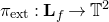 $\pi _{\mathrm {ext}}: {\mathbf {L}_{f}} \to \mathbb {T}^2$
the projection onto the first coordinate. The map
 \begin{align*} {\hat {f}}: {\mathbf {L}_{f}} & \to {\mathbf {L}_{f}} \\ (x_0, x_1, x_2, \ldots ) & \mapsto (f(x_0), x_0, x_1, \ldots ) \end{align*}
is then a homeomorphism on
 $\mathbf {L}_{f}$
satisfying
 $\pi _{\mathrm {ext}} \circ {\hat {f}} = f \circ \pi _{\mathrm {ext}}$
. In the case where
 $f$
is a self-cover (as is the case for local diffeomorphisms), the set
 $\mathbf {L}_{f}$
has an interesting structure: it is a solenoidal
 $2$
-manifold, meaning that it is locally homeomorphic to the product of a two-dimensional disk with a Cantor set. More specifically,
 $\mathbf {L}_{f}$
is a fiber bundle whose fibers
 $\pi _{\mathrm {ext}}^{-1}(x)$
are Cantor sets. This structure will be of importance when proving the continuity of Lyapunov exponents (§ 4), and is explained in some detail in Appendix A.
Given any
 $f$
-invariant Borel measure
 $\mu$
on
 $\mathbb {T}^2$
, there exists a unique
 $\hat {f}$
-invariant Borel measure
 $\hat {\mu }$
on
 $\mathbf {L}_{f}$
such that
 $(\pi _{\mathrm{ext}})_* {\hat {\mu }} = \mu$
. This is called the
 $\textit {lift}$
of
 $\mu$
. According to Rokhlin’s disintegration theorem,
 $\hat {\mu }$
can be disintegrated along the partition into fibers
 $\{\pi _{\mathrm {ext}}^{-1}(x): x \in \mathbb {T}^2 \}$
, yielding a family of conditionals. These conditionals are determined by their measures on cylinders in the following way.
Proposition 2.1.
Let
 $\mu$
be the Haar measure on
 $\mathbb {T}^2$
and
 $\hat {\mu }$
its lift on
 $\mathbf {L}_{f}$
. Then
 \begin{equation} {\hat {\mu }}(A) = \int {\hat {\mu }}_x(A) \, d\mu (x), \end{equation}
for every Borel set
 $A \subset {\mathbf {L}_{f}}$
, where
 ${\hat {\mu }}_x$
is the unique measure on
 $\pi _{\mathrm {ext}}^{-1}(x)$
satisfying
 \begin{equation} {\hat {\mu }}_x(\{(\xi _0, \xi _1, \ldots ) \in \pi _{\mathrm {ext}}^{-1}(x): \xi _i = x_i\}) = |\!\det Df^i(x_i)|^{-1}. \end{equation}
We refer to Appendix A.5 for a proof.
2.2 Lyapunov exponents for the natural extension
Given a cocycle
 $A:X\to \textrm {GL}_2({\mathbb {R}})$
over a map
 $h:X\to X$
, we denote, for
 $x\in X, v\in {\mathbb {R}^2}\setminus \{0\}$
,
 \begin{align*} \chi _{(h,A)}(x,v)&=\lim _{n\to +\infty }\frac {\log \Vert A^{(n)}(x)\cdot v\Vert }{n},\\[5pt] \chi _{(h,A)}^+(x)&=\lim _{n\to +\infty }\frac {\log \Vert A^{(n)}(x)\Vert }{n},\\[5pt] \chi _{(h,A)}^-(x)&=\lim _{n\to +\infty }\frac {\log \mathrm {m}\big(A^{(n)}(x)\big)}{n}, \end{align*}
provided that these limits exist.
The differential of the endomorphism
 $f:\mathbb {T}^2\to \mathbb {T}^2$
defines a cocycle over
 $f$
, and we denote the associated exponents by
 $\chi _f(x,v), \chi _f^{+}(x), \chi _f^{-}(x)$
. We also define a cocycle
 $D{\hat {f}}$
over
 $\hat {f}$
by
 \begin{equation*} D_{\hat {x}}{\hat {f}}=D_{x_0}f, \end{equation*}
where
 $\hat {x}=(x_n)_{n\geq 0}$
, which behaves naturally and, in particular, with the usual notation,
 \begin{align*} D_{\hat {x}}{\hat {f}}^{(n)}=\begin{cases} D_{{\hat {f}}^{n-1}\hat {x}}{\hat {f}}\circ \cdots D_{{\hat {f}}\hat {x}}{\hat {f}}\circ D_{\hat {x}}{\hat {f}}, & n\gt 0,\\[5pt] \mathrm{Id}, & n=0,\\[5pt] (D_{{\hat {f}}^{-n}\hat {x}}{\hat {f}})^{-1}\circ \cdots (D_{{\hat {f}}^{-2}\hat {x}}{\hat {f}})^{-1}\circ (D_{{\hat {f}}^{-1}\hat {x}}{\hat {f}})^{-1}, & n\lt 0, \end{cases} \end{align*}
one gets, by the chain rule,
 $D_{\hat {x}}{\hat {f}}^{(n)}=D_{\hat {x}}({\hat {f}}^{n})$
, i.e.
 \begin{align*} D_{\hat {x}}{\hat {f}}^n=\begin{cases} D_{x_0}f^n, & n\gt 0,\\ \mathrm{Id}, & n=0,\\ (D_{x_n}f^n)^{-1}, & n\lt 0. \end{cases} \end{align*}
The exponents of this cocycle are denoted by
 $\chi _{{\hat {f}}}(\hat {x},v), \chi _{{\hat {f}}}^{+}(\hat {x}), \chi _{{\hat {f}}}^{-}(\hat {x})$
. From the formula above it is evident that
 \begin{align*} \chi _f(\pi _{\mathrm {ext}}(\hat {x}),v)&=\chi _{{\hat {f}}}(\hat {x},v),\\[3pt] \chi _f^{+}(\pi _{\mathrm {ext}}(\hat {x}))&=\chi _{{\hat {f}}}^{+}(\hat {x}),\\[3pt] \chi _f^{-}(\pi _{\mathrm {ext}}(\hat {x}))&=\chi _{{\hat {f}}}^{-}(\hat {x}); \end{align*}
that is, if one quantity is defined then the other is defined as well and the two coincide. We can now apply Oseledets’ theorem (see, for example, the discussion in [Reference RuelleRue79]) to the cocycle
 $D{\hat {f}}$
, and use the fact that these coincide almost everywhere with minus the exponents of
 $D{\hat {f}}^{-1}$
, and hence, from the discussion above, we can compute the exponents of
 $f$
using
 ${\hat {f}}^{-1}$
. Together with the decomposition of
 $\hat {\mu }$
in terms of
 $\{{\hat {\mu }}_x\}$
given in Proposition 2.1, we get the following facts, which for convenience we record below.
Lemma 2.1.
There exists a completely
 $\hat {f}$
-invariant set
 $\hat {\mathcal {R}} \subset {\mathbf {L}_{f}}$
of full
 $\hat {\mu }$
measure such that, for every
 $\hat {x}\in \hat {\mathcal {R}}, x=\pi _{\mathrm {ext}}(\hat {x})$
, the following hold:
-
(1)
$\chi _{{\hat {f}}}^{+}(\hat {x})=-\chi _{{\hat {f}}^{-1}}^{-}(\hat {x})=\chi ^+_f(x)$
; -
(2)
$\chi _{{\hat {f}}}^{-}(\hat {x})=-\chi _{{\hat {f}}^{-1}}^{+}(\hat {x})=\chi ^-_f(x)$
.


Moreover, there exists a completely
 $f$
-invariant set
 $\mathcal {R} \subset \pi _{\mathrm {ext}}(\hat {\mathcal {R}})$
of full
 $\mu$
measure such that, for every
 $x\in \mathcal {R}$
,
 ${\hat {\mu }}_x(\hat {\mathcal {R}})=1$
.
In fact, from Oseledets’ theorem it also follows that, for
 $\hat {x} \in \hat {\mathcal {R}}$
, there exist subspaces
 $E^{-}_{\hat {x}}, E^{+}_{\hat {x}}$
of
 $\mathbb {R}^2$
such that, for
 $v\in E^{\pm }_{\hat {x}}\setminus \{0\}$
,
 \begin{equation*} \chi _{{\hat {f}}}^{\pm }(\hat {x})=\chi _{{\hat {f}}}(\hat {x},v)=-\chi _{{\hat {f}}^{-1}}(\hat {x},v)=-\chi _{{\hat {f}}^{-1}}^{\mp }(\hat {x}). \end{equation*}
Remark 2.1. The bundle
 $(\pi _{\mathrm {ext}})_{*}E^{-}$
defines a measurable bundle over
 $\mathcal {R}$
, since it depends only on the forward orbit of the point. However,
 $E^{+}$
does not project under
 $\pi _{\mathrm {ext}}$
to a bundle on
 $\mathbb {T}^2$
because
 $E^{+}$
may be different at different points on the same fiber.
2.3 Relation between Lyapunov exponents and
$C_{\chi }(f), C_{\det }(f)$

The strategy for the proof of Theorem A is to estimate
 $\chi _{{\hat {f}}^{-1}}^{+}$
. More precisely, we want to get explicit lower bounds for
 \begin{equation*}\int _{\pi _{\mathrm{ext}}^{-1}(x)} \chi _{{\hat {f}}^{-1}}^{+}\ d{\hat {\mu }}_x, \end{equation*}
at
 $\mu$
-almost every (a.e.)
 $x \in \mathbb {T}^2$
, which by the previous Lemma gives us analogous bounds for
 $\chi ^+_f(x)$
and
 $\chi ^-_f(x)$
 $\mu$
-almost everywhere.
Recall the definition of
 $I(x,v;f^n)$
from (1). Using the description of the disintegrations of
 ${\hat {\mu }}_x$
from Proposition 2.1, we obtain that, for
 $x\in \mathbb {T}^2$
and a unit vector
 $v\in \mathbb S^1\subset {\mathbb {R}^2}$
(or equivalently any
 $(x,v)\in T^1\mathbb {T}^2$
),
 \begin{equation} I(x,v;f^n)=\sum _{y\in f^{-n}(x)}\frac {\log \|(D_yf^n)^{-1}v\|}{|\!\det (D_yf^n)|}=\int _{\pi _{\mathrm{ext}}^{-1}(x)} \log \big\Vert D_{{\hat {y}}}{\hat {f}}^{-n}(v)\big\Vert \ d{\hat {\mu }}_x({\hat {y}}). \end{equation}
Let us fix the following notation. For any unit tangent vector
 $(x,v)$
at
 $x\in \mathbb {T}^2$
and for any
 $y\in f^{-i}(x)$
, we define
 $F_y^{-i}v= {(D_yf^i)^{-1}v}/{\|(D_yf^i)^{-1}v\|}$
, so that
 $(y,F_y^{-i}v)$
is the unit tangent vector at
 $y$
obtained by pulling back
 $v$
under
 $Df^i$
and normalizing.
Lemma 2.2.
For any
 $n\in \mathbb N$
we have
 \begin{equation*} I(x,v;f^n)=\sum _{i=0}^{n-1}\sum _{y\in f^{-i}(x)}\frac 1{|\!\det (D_yf^i)|}I(y,F_y^{-i}v;f). \end{equation*}
In other words,
 $(1/n)I(x,v;f^n)$
is a convex combination of other
 $I(y,w;f)$
.
Proof.
We will argue by induction. Assume that the formula holds for
 $n$
, so then
 \begin{align*} I(x,v;f^{n+1})&=\sum _{y\in f^{-n-1}(x)}\frac {\log \|(D_yf^{n+1})^{-1}v\|}{|\!\det (D_yf^{n+1})|}\\[5pt] &=\sum _{y\in f^{-n}(x)}\sum _{z\in f^{-1}(y)}\frac {\log \|(D_zf)^{-1}(D_yf^n)^{-1}v\|}{|\!\det (D_zf)\det (D_yf^n)|}\\[5pt] &=\sum _{y\in f^{-n}(x)}\sum _{z\in f^{-1}(y)}\frac {\log \|(D_zf)^{-1}F_y^{-n}v\|+\log \|(D_yf^n)^{-1}v\|}{|\!\det (D_zf)\det (D_yf^n)|}\\[5pt] &=\sum _{y\in f^{-n}(x)}\frac 1{|\!\det (D_yf^n)|}\sum _{z\in f^{-1}(y)}\frac {\log \|(D_zf^{n})^{-1}F_y^{-n}v\|}{|\!\det (D_zf)|}\\[5pt] &\quad +\sum _{y\in f^{-n}(x)}\frac {\log \|(D_yf^n)^{-1}v\|}{|\!\det (D_yf^n)|}\sum _{z\in f^{-1}(y)}\frac 1{|\!\det (D_zf)|}\\[5pt] &=\sum _{y\in f^{-n}(x)}\frac 1{|\!\det (D_yf^n)|}I(y,F_y^{-n}v;f)+\sum _{y\in f^{-n}(x)}\frac {\log \|(D_yf^n)^{-1}v\|}{|\!\det (D_yf^n)|}\\[5pt] &=I(x,v;f^n)+\sum _{y\in f^{-n}(x)}\frac 1{|\!\det (D_yf^n)|}I(y,F_y^{-n}v;f). \end{align*}
This concludes the proof of the formula.
Observe that the sum of the coefficients of
 $\sum _{y\in f^{-i}(x)} (1/{|\!\det (D_yf^i)|})I(y,F_y^{-i}v;f)$
is equal to one for every
 $i$
, so the sum of the coefficients of
 $I(x,v;f^n)$
is equal to
 $n$
. Then indeed
 $(1/n)I(x,v;f^n)$
is a convex combination of other
 $I(y,w;f)$
.
Corollary 2.1.
For any
 $(x,v)\in T^1\mathbb {T}^2$
and any natural numbers
 $n,m$
, we have that
 $(1/n)I(x,v;f^{nm})$
is a convex combination of other
 $I(y,w;f^m)$
.
Remember that
 \begin{equation*} C_{\chi }(f)=\sup _{m\in \mathbb N}\frac 1m\inf _{(x,v)\in T^1\mathbb {T}^2}I(x,v;f^m). \end{equation*}
A straightforward consequence of the definition and of Corollary 2.1 is that the definition of
 $C_{\chi }(f)$
is actually independent of the election of the norm on
 $T\mathbb {T}^2$
, and can be rewritten as
 \begin{equation*} C_{\chi }(f)=\lim _{m\rightarrow \infty }\frac 1m\inf _{(x,v)\in T^1\mathbb {T}^2}I(x,v;f^m). \end{equation*}
We also have that
 \begin{equation*} C_{\det }(f)=\sup _{n\in \mathbb N}\frac 1n\inf _{x\in M}\log (|\!\det (Df_x^n)|)=\lim _{n\rightarrow \infty } \frac 1n \inf _{x\in M}\log (|\!\det (Df_x^n)|). \end{equation*}
The following proposition gives bounds on the Lyapunov exponents at almost every point in terms of
 $C_{\chi }(f)$
and
 $C_{\det }(f)$
, and establishes the first part of Theorem A.
Proposition 2.2.
For
 $\mu$
-a.e.
 $x\in \mathbb {T}^2$
we have
 $\chi ^{-}_f(x)\leq -C_{\chi }(f)$
and
 $\chi ^{+}_f(x)\geq C_{\chi }(f)+C_{\det }(f)$
. In particular:
-
(1) if
$C_{\chi }(f)\gt 0$
(
$f\in \mathcal U$
), then
$\chi _f^-(x)\lt 0\lt \chi _f^+(x)$
for almost every
$x\in \mathbb {T}^2$
; -
(2) if
$C_{\chi }(f)\gt - \tfrac{1}{2}C_{\det }(f)$
(
$f\in \mathcal U_1$
), then
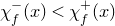
$\chi _f^-(x)\lt \chi _f^+(x)$
for almost every
$x\in \mathbb {T}^2$
.







Proof.
Observe that for
 $\mu$
-a.e.
 $x\in \mathbb {T}^2$
we have
 \begin{equation*} \chi ^{+}_f(x)+\chi ^{-}_f(x)=\lim _{n\rightarrow \infty }\frac 1n \log |\!\det D_xf^n|\geq C_{\det }(f), \end{equation*}
and thus if
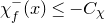 $\chi ^{-}_f(x)\leq -C_{\chi }$
 $\mu$
-almost everywhere, this immediately implies that also
 $\chi ^{+}_f(x)\geq C_{\chi }(f)+C_{\det }(f)$
.
Let
 $C_m= (1/m)\inf _{(x,v)\in T^1\mathbb {T}^2}I(x,v;f^m)$
. From Corollary 2.1 we have that, for every
 $n,m\geq 1$
and unit tangent vector
 $(x,v)$
,
 \begin{equation*} \frac {I(x,v;g^{nm})}{nm}=\frac {1}{nm}\int _{\pi _{\mathrm{ext}}^{-1}(x)} \log \left \Vert D_{{\hat {y}}}{\hat {f}}^{-nm}v\right \Vert \ d{\hat {\mu }}_x({\hat {y}})\geq C_m. \end{equation*}
By Lemma 2.1 and the dominated convergence theorem it follows that, for almost every
 $x$
and any unit vector
 $v$
,
 \begin{equation*} \int _{\pi _{\mathrm{ext}}^{-1}(x)} \chi _{{\hat {f}}^{-1}}({\hat {y}},v)\ d{\hat {\mu }}_x({\hat {y}})\geq C_m, \end{equation*}
and therefore
 \begin{align*} -\chi ^-_f(x)&=\int _{\pi _{\mathrm{ext}}^{-1}(x)} \chi _{{\hat {f}}^{-1}}^{+}({\hat {y}})\ d{\hat {\mu }}_x({\hat {y}})\geq \int _{\pi _{\mathrm{ext}}^{-1}(x)} \chi _{{\hat {f}}^{-1}}({\hat {y}},v)\ d{\hat {\mu }}_x({\hat {y}})\geq \sup _{m\in \mathbb N}C_m\\ &=C_{\chi }(f). \end{align*}
Remark 2.2. Let us make some remarks on the constant
 $C_{\chi }(f)$
and the NUH property. The fact that we have a negative exponent
 $\chi ^-(\hat {x})\leq -\chi$
at
 $\hat {\mu }$
-a.e. point is equivalent to the fact that, for
 $\mu$
-a.e.
 $x\in \mathbb {T}^2$
and for all unit vectors
 $v$
with the possible exception of countably many vectors, we have
 \begin{equation*} \lim _{n\rightarrow \infty }\frac 1nI(x,v;f^n)\geq \chi . \end{equation*}
The possible exceptional vectors come from the possibility of having the following degenerate situation: the
 $E^+(\hat {x})$
spaces coincide for a set of positive
 $\hat {\mu }_x$
measures on the fiber
 $\pi _{\mathrm{ext}}^{-1}(x)$
.
In other words, the NUH property with uniform bound on the exponents is equivalent to
 \begin{equation*} C_{\chi }'(f)= \mathop{ess\,inf}\limits_{(x,v)\in T^1\mathbb {T}^2}\left (\lim _{n\rightarrow \infty }\frac 1nI(x,v;f^n)\right )\geq \chi \gt 0, \end{equation*}
where
 $C_{\chi }'(f)\gt C_{\chi }(f)$
would be an optimal bound. We could reformulate the results using
 $C_{\chi }'(f)$
and a similar
 $C_{\det }'(f)$
instead of
 $C_{\chi }(f)$
and
 $C_{\det }(f)$
, but these constants seem to be difficult to estimate, and may not depend semi-continuously on
 $f$
, so the corresponding sets of endomorphisms would not be open.
Suppose that, furthermore,
 $E^+$
is independent of the past: for
 $\mu$
-a.e.
 $x$
, for any subspace
 $E\subset \mathbb R^2$
,
 $\hat {\mu }_x\left (\{\hat {x}\in \pi _{\mathrm{ext}}^{-1}(x):\ E^+(\hat {x})=E\}\right )=0$
. Then, for
 $\mu$
-a.e.
 $x\in \mathbb {T}^2$
and for any unit vector
 $v$
we have
 \begin{equation*} \lim _{n\rightarrow \infty }\frac 1nI(x,v;f^n)\geq \chi . \end{equation*}
Remark 2.3. As we mentioned before, a related approach for establishing the positivity of the top Lyapunov exponent (with respect to the stationary measure) in the context of random surface diffeomorphisms appears in [Reference ChungChu20, Reference LiuLiu16].
2.4 Some algebra
Denote
 \begin{align} \mathscr {H}_{NH}(\mathbb {T}^2)=\{E\in \mathrm {M}_{2 \times 2}(\mathbb {Z}):\det E \neq 0, E\neq k\cdot \mathrm{Id}, k\in \mathbb {Z}\}. \end{align}
For
 $E\in \mathscr {H}_{NH}(\mathbb {T}^2)$
, let
 $\tau _1(E)$
be the largest common factor of the entries of
 $E$
; that is,
 \begin{align} \tau _1(E) = \max \{ k \in \mathbb {N}: E = k\cdot G \text { for some }G \in \mathrm {M}_{2 \times 2}(\mathbb {Z})\}. \end{align}
Let
 $\tau _2(E) = |\!\det (E)|/\tau _1(E)$
: then
 $\tau _2(E)$
is an integer, and since
 $E=\tau _1(E)\cdot G$
for some integer matrix
 $G$
,
 $|\!\det (E)|=\tau _1(E)^2|\!\det (G)|$
and
 $\tau _1(E) | \tau _2(E)$
. The numbers
 $\tau _1(E), \tau _2(E)$
are the elementary divisors of
 $E$
. The quantity
 \begin{equation*} \mathrm {d}=|\!\det E |= \tau _1\cdot \tau _2 \end{equation*}
coincides with the topological degree of the induced endomorphism
 $E:\mathbb {T}^2\to \mathbb {T}^2$
. We need the following result from linear algebra (see, for example, [Reference JacobsonJac09]).
Theorem 2.1 (Smith Normal Form). There exist
 $L, R \in \textrm {GL}_2(\mathbb {Z})$
such that
 $E = L\cdot D\cdot R$
, where
 \begin{equation*}D = \bigg(\begin{matrix} \tau _1 & \quad 0 \\[2pt] 0 & \quad \tau _2 \end{matrix} \bigg ) .\end{equation*}
For
 $E:\mathbb {T}^2\to \mathbb {T}^2$
, the pre-images of
 $x\in \mathbb {T}^2$
are of the form
 \begin{equation*} E^{-1}(x)=y+\pi _{\mathrm {cov}}(E^{-1}({\mathbb {Z}^2})), \end{equation*}
where
 $E(y)=x$
: we are thus interested in understanding the lattice
 $E^{-1}({\mathbb {Z}^2})$
.
Proposition 2.3.
With the hypotheses above, there exists
 $P \in \textrm {GL}_2(\mathbb {Z})$
such that the matrix
 $G = P^{-1}\cdot E \cdot P$
satisfies
 \begin{equation} G^{-1}({\mathbb {Z}^2}) = \bigg \{ \bigg ( \begin{matrix} ({i}/{\tau _2}) \\[5pt] ({j}/{\tau _1}) \end{matrix} \bigg ) : i, j \in \mathbb {Z} \bigg \}. \end{equation}
Moreover, if
 $E$
is not a homothety, then
 $P$
may be chosen so that
 $e_2=(0,1)$
is not an eigenvector of
 $G$
.
Proof.
Let
 $L,R \in \textrm {GL}_2(\mathbb {Z})$
be such that
 $E = L\cdot D\cdot R$
, where
 $D$
is the Smith Normal Form of
 $E$
. Denote by
 \begin{equation*}J = \bigg ( \begin{matrix} 0 & \quad 1 \\[2pt] 1 & \quad 0 \end{matrix}\bigg ) \end{equation*}
the involution which permutes
 $e_1$
and
 $e_2$
, and let
 $P = R^{-1}J$
. We claim that the matrix
 $G = P^{-1}\cdot E\cdot P$
satisfies (10). Indeed,
 $G$
can be written as
 \begin{equation*} G = J\cdot R\cdot L\cdot D\cdot R\cdot R^{-1}\cdot J = J\cdot R\cdot L\cdot D\cdot J = M\cdot D\cdot J, \end{equation*}
where
 $M = J\cdot R\cdot L\in \textrm {GL}$
. Hence
 \begin{equation*} G^{-1}({\mathbb {Z}^2}) = J^{-1}D^{-1}({\mathbb {Z}^2}), \end{equation*}
which is clearly in the form expressed in (10).
If we further assume that
 $E\in \mathscr {H}_{NH}(\mathbb {T}^2)$
, then it has at most two eigenvectors in
 $\mathbb {Z}^2$
. In particular, there is some
 $k \in \mathbb {Z}$
such that
 $k\cdot e_1+e_2$
is not an eigenvector of
 $E$
. Let
 \begin{equation*}S = \left (\begin{matrix} 1 & \quad k \\[2pt] 0 & \quad 1 \end{matrix} \right ),\end{equation*}
and take
 $ P' = P\cdot S$
. It follows that
 $e_2$
is not an eigenvector of
 \begin{equation*} G' = {P'}^{-1}\cdot E \cdot P' = S^{-1}\cdot G\cdot S. \end{equation*}
Moreover, since
 $\tau _1$
divides
 $\tau _2$
,
 $S$
acts as a permutation on
 $G^{-1}({\mathbb {Z}^2})$
. Hence (10) holds with
 $G'$
in place of
 $G$
.
3. Construction of non-uniformly hyperbolic endomorphisms
In this section we will show that
 $\mathcal U$
has elements in almost all the homotopy classes of endomorphisms.
3.1 Endomorphisms
Fix
 $E\in \mathscr {H}_{NH}(\mathbb {T}^2)$
with elementary divisors
 $\tau _1, \tau _2$
, and denote by
 $\mathrm {d}=\tau _1\cdot \tau _2$
its degree. We assume that
 $\tau _2\geq 5$
. By making the linear change of coordinates indicated in Proposition 2.3 we can assume that
 ${\mathbb {P}} E$
does not fix
 $[(0,1)]$
and
 $E^{-1}\mathbb Z^2= (1/{\tau _2})\mathbb Z\times 1/{\tau _1}\mathbb Z$
.
Let
 $\delta \lt 1/{4\tau _2}$
. Choose points
 $x_1,x_2,x_3,x_4\in \mathbb T^1$
, in this order, such that:
-
–
$I_1=[x_1,x_2]$
and
$I_3=[x_3,x_4]$
have size
$2\delta$
; -
– the translation of
$I_1$
by a multiple of
$1/{\tau _2}$
does not intersect
$I_3$
; -
–
$I_2=(x_2,x_3)$
and
$I_4=(x_4,x_1)$
have size strictly larger than
$(1/{\tau _2}) \left [({\tau _2-1})/2\right ]$
.Footnote
4



Remark 3.1. If
 $\tau _2$
is odd then the points can be
 $\{1/4-\delta ,1/4+\delta , 3/4-\delta ,3/4+\delta \}$
.
Definition 3.1.
-
(1) The critical region is
$\mathcal {C}=(I_1\cup I_3)\times \mathbb T^1\subset \mathbb {T}^2$
, and its complement
$\mathcal G$
is the good region. -
(2) The good region is divided into
$\mathcal G^+=I_4\times \mathbb T^1$
and
$\mathcal G^-=I_2\times \mathbb T^1$
.




Remark 3.2. Observe that
 $\mathcal C$
is closed and
 $\mathcal G^+$
and
 $\mathcal G^-$
are open.
Lemma 3.1.
For every
 $x\in \mathbb {T}^2$
,
 $E^{-1}(x)$
has
 $\mathrm {d}$
points. At least
 $\tau _1\left [({\tau _2-1})/2\right ]$
pre-images are inside each of
 $\mathcal G^+$
and
 $\mathcal G^-$
, and at most
 $\tau _1$
of them are inside
 $\mathcal C$
.
Furthermore, at least one pre-image of
 $x$
is inside
 $\mathcal G$
, and
 $d(x,\mathcal C)\gt 1/{10}$
.
Proof.
The first part follows from Proposition 2.3 and the construction of the regions. The last statement is a consequence of the fact that at least one good region has size greater than
 ${(1-4\delta })/2\gt ({\tau _2-1})/{2\tau _2}$
, and if we take a band of size
 $ 1/{\tau _2}$
in the middle of this good region, at least one pre-image has to fall in the middle band. Then the distance to the boundary is greater than
 $\tfrac{1}{2}\left (({\tau _2-1})/{2\tau _2}- 1/{\tau _2}\right )= ({\tau _2-3})/{4\tau _2}\geq 1/{10}$
because
 $\tau _2\geq 5$
.
3.2 Shears
We start studying the dynamics of a family of shears that we will use to deform the original endomorphism. Let
 $s:\mathbb T^1\rightarrow \mathbb R$
. Consider the family of conservative diffeomorphisms of the torus
 \begin{equation} h_t(x_1,x_2)=(x_1, x_2+ts(x_1)). \end{equation}
Remark 3.3. If
 $U:\mathbb {T}^2\to \mathbb {T}^2$
is the Dehn twist given by
 $U(x_1,x_2)=(x_1+x_2,x_1)$
, and
 $s(x_1)=\sin (2\pi x_1)$
, then
 $\{s_t=U\circ h_t\}_{t\gt 0}$
is the famous standard family [Reference Chirikov and ShepelyanskyCS08] and has the formula
 $s_t(x_1,x_2)=(x_1+x_2+t\sin (2\pi x_1), x_2+t\sin (2\pi x_1))$
.
We observe that
 \begin{equation} D_{(x_1,x_2)}h_t=\bigg(\begin{matrix} 1 & \quad 0\\[3pt] ts'(x_1) & \quad 1 \end{matrix}\bigg). \end{equation}
As we mentioned before,
 $C_{\chi }(f)$
is independent of the choice of the norm on the tangent bundle of
 $\mathbb {T}^2$
. In order to simplify the computations, we will choose the maximum norm:
 \begin{equation*} \|(v_1,v_2)\|=\max \{|v_1|,|v_2|\}. \end{equation*}
All the computations in this section are performed using this norm. We will try to keep track of the constants involved; this will make the exposition a bit more technical but will help us to give some concrete examples in § 3.5.
A first observation is the following:
 \begin{equation*} \left \|\begin{pmatrix} 1 & \quad 0\\ a & \quad 1\\ \end{pmatrix}\right \|= 1\bigg/\left({\mathrm {m}\left (\begin{pmatrix} 1 & \quad 0\\ a & \quad 1\\ \end{pmatrix}\right )}\right)=a+1. \end{equation*}
Let
 $0\lt a\lt b$
. There exists an analytic map
 $s$
which satisfies the following conditions:
-
(1) If
$u\in I_4$
then
$a\lt s'(u)\lt b$
; -
(2) If
$u\in I_2$
then
$-b\lt s'(u)\lt -a$
; -
(3) If
$u\in I_1\cup I_3$
then
$|s'(u)|\lt b$
.





Remark 3.4. If
 $\tau _2$
is odd, then in view of Remark
3.1 we can take
 $s(u)=\sin (2\pi u)$
, with
 $a=2\pi \sin (2\pi \delta )-\epsilon$
and
 $b=2\pi +\epsilon$
, for any
 $\epsilon \gt 0$
.
As a consequence we get, for every
 $x\in \mathbb {T}^2$
,
 \begin{align} \|D_xh_t\|= \frac{1}{{\mathrm {m}\left (D_xh_t\right )}}\lt bt+1. \end{align}
Definition 3.2. Given any
 $\alpha \gt 0$
, the corresponding horizontal cone is
 $\Delta _{\alpha }^h=\{(u_1,u_2)\in {\mathbb {R}}^2: |u_2|\leq \alpha |u_1|\}$
, while the corresponding vertical cone is its complement
 $\Delta _{\alpha }^v={\mathbb {R}}^2\setminus \Delta _{\alpha }^h$
.
Since
 $E$
does not fix the vertical vector
 $(0,1)$
, there exists
 $\alpha \gt 1$
such that
 $E^{-1}\Delta _{\alpha }^v\subset \overline {E^{-1}\Delta _{\alpha }^v}\subset \textrm{Int}(\Delta _{\alpha }^h)\subset \Delta _{\alpha }^h$
, and from now on we fix such an
 $\alpha$
. Observe that
 $\Delta _{\alpha }^v$
is open and
 $\Delta _{\alpha }^h$
is closed.
Remark 3.5. For a Dehn twist (eventually multiplied with a homothety) we have
 $\alpha =2+\epsilon$
.
Lemma 3.2.
For every
 $t\gt {2\alpha }/a$
and for every unit vector
 $v\in T_x\mathbb {T}^2$
the following holds.
-
(1) If
$v\in \Delta _{\alpha }^h$
and
-
(a)
$x\in \mathcal G$
, then
-
–
$(D_xh_t)^{-1}v\in \Delta _{\alpha }^v$
(
$D_xh_t^{-1}\Delta _{\alpha }^h\subset \Delta _{\alpha }^v$
),
-
–
$\Vert (D_xh_t)^{-1}v\Vert \gt {({at-\alpha })}/{\alpha }= t((a-(\alpha/t))\alpha)$
;
-
-
(b)
$x\in \mathcal C$
, then
-
–
$\Vert (D_xh_t)^{-1}v\Vert \gt {1}/{\alpha }$
.
-
-
-
(2) If
$v=\pm (v_1,1)\in \Delta _{\alpha }^v$
then
-
(a) either for every
$x\in \mathcal G^+$
(if
$v_1\leq 0$
) or for every
$x\in \mathcal G^-$
(if
$v_1\geq 0$
) the following hold:
-
–
$(D_xh_t)^{-1}v\in \Delta _{\alpha }^v$
, -
–
$\Vert (D_xh_t)^{-1}v\Vert \gt 1$
;
-
-
(b) for all the other
$x$
, we have
-
–
$\Vert (D_xh_t)^{-1}v\Vert \gt {1}/({bt+1})$
.
-
-














Proof.
For the boundary vectors
 $v=(1,\alpha ), w=(1,-\alpha )$
we compute
 \begin{align*} (D_xh_t)^{-1}v=(1,-ts'(x_1) +\alpha ),\quad (D_xh_t)^{-1}w=(1,-ts'(x_1) -\alpha ). \end{align*}
It follows that if
 $x\in \mathcal {G}$
then
 \begin{equation*} |{-}ts'(x_1) +\alpha |\geq ta-\alpha \gt \alpha \end{equation*}
if
 $t\gt {2\alpha }/a$
. The same is true for
 $w$
, which shows that
 $(D_xh_t)^{-1}\Delta _{\alpha }^h\subset \Delta _{\alpha }^v$
.
We also remark that the minimal expansion of
 $D_xh_t^{-1}$
on
 $\Delta _{\alpha }^h$
for
 $x\in \mathcal G$
is realized on
 $v$
or on
 $w$
. Then for every
 $v\in \Delta _{\alpha }^h$
and for every
 $x\in \mathcal {G}$
we have
 \begin{equation*} \Vert (D_xh_t)^{-1}v\Vert \gt \frac{\|(1,ta-\alpha )\|}{\|(1,\alpha )\|}\geq \frac{ta-\alpha }{\alpha }. \end{equation*}
Part (b) is similar and left as an exercise.
The last part follows by noting that
 $s'$
has constant sign in
 $\mathcal {G}^+, \mathcal {G}^-$
, and
 \begin{equation*} \mathrm {m}((D_xh_t)^{-1})= \frac{1}{{\|D_xh_t\|}}\gt \frac{1}{bt+1},\quad \forall x\in \mathbb {T}^2. \end{equation*}
3.3 Endomorphisms and shears
We now consider the analytic maps
 \begin{equation*} f_t=E\circ h_t; \end{equation*}
clearly
 $f=f_t$
is an area-preserving endomorphism isotopic to
 $E$
.
The regions
 $\mathcal C$
,
 $\mathcal G^+$
and
 $\mathcal G^-$
are invariant under
 $h_t$
, and furthermore
 $\mathcal C$
is closed while
 $\mathcal G^+$
and
 $\mathcal G^-$
are open. A direct consequence of Lemma 3.1 is the following.
Lemma 3.3.
For every
 $x\in \mathbb {T}^2$
,
 $f^{-1}(x)$
has
 $\mathtt {d}$
points. At least
 $\tau _1[{(\tau _2-1)}/2]$
pre-images are inside each one of
 $\mathcal G^+$
and
 $\mathcal G^-$
, and at most
 $\tau _1$
of them are inside
 $\mathcal C$
.
Furthermore, at least one pre-image of
 $x$
is inside
 $\mathcal G$
and
 $d(x,\mathcal C)\gt 1/{10}$
.
Let
 $e_v=\inf _{v\in \Delta _{\alpha }^v,\ \|v\|=1}\|E^{-1}v\|$
,
 $e_h=\inf _{v\in \Delta _{\alpha }^h,\ \|v\|=1}\|E^{-1}v\|$
. From Lemma 3.2 we get the following lemma.
Lemma 3.4.
For
 $t\gt {2\alpha }/a$
the following hold.
-
(1) If
$x\in \mathcal G$
then
$(D_xf)^{-1}\Delta _{\alpha }^v\subset \overline {(D_xf)^{-1}\Delta _{\alpha }^v}\subset \Delta _{\alpha }^v$
(it is strictly invariant).
-
(2) If
$v\in \Delta _{\alpha }^v$
is a unit vector, then
\begin{align*} \|(D_xf)^{-1}v\|\gt \begin{cases} \dfrac {e_v\left(a-({\alpha }/t)\right)}{\alpha } t, & x\in \mathcal {G},\\[6pt] \dfrac {e_v}{\alpha }, & x\in \mathcal {C}. \end{cases} \end{align*}
-
(3) If
$v\in \Delta _{\alpha }^h$
and
$E^{-1}v=(v_1,v_2)$
, let
$*(v)$
be the sign of
$- {v_1}/{v_2}$
(0 and
$\pm \infty$
have both + and – signs). Then for all
$x\in \mathcal G^{*(v)}$
we have
$(D_xf)^{-1}(v)\in \Delta _{\alpha }^v$
. -
(4) If
$v\in \Delta _{\alpha }^h$
is a unit vector, then
\begin{align*} \|(D_xf)^{-1}v\|\gt \begin{cases} e_h, & x\in \mathcal G^{*(v)},\\[6pt] \dfrac {e_h}{b+(1/t)}t^{-1}, & x\notin \mathcal G^{*(v)}. \end{cases} \end{align*}










3.4 Non-uniform hyperbolicity
In this part we will establish the remaining part of Theorem A and prove that, for
 $t$
sufficiently large, the map
 $f=f_t$
is NUH. The arguments are inspired by the abstract methods used in [Reference Carrasco and SaghinCS22] (see also [Reference CarrascoCar20]), but with the additional difficulty that we have to work in the natural extension instead of directly in the manifold. We rely on Proposition 2.2.
Proof of Theorem A. (
 $\mathcal U$
intersects the isotopy class of
 $E$
). For any
 $(x,v)\in T\mathbb {T}^2, v\neq 0$
and
 $n\geq 0$
, denote by
 $Df^{-n}(x,v)$
all the pre-images of
 $(x,v)$
under
 $Df$
:
 \begin{equation*}Df^{-n}(x,v)=\{(y,w)\in T\mathbb {T}^2:\ f^n(y)=x,\ D_yf^nw=v\}.\end{equation*}
For any nonzero tangent vector
 $(x,v)$
, define
 \begin{align} &\mathcal {G}_n=\{(z,w)\in Df^{-n}(x,v):\ w\in \Delta _{\alpha }^v\},\\[-9pt]\nonumber \end{align}
 \begin{align} &\mathcal {B}_n=Df^{-n}(x,v)\setminus \mathcal G_n,\\[-9pt]\nonumber \end{align}
 \begin{align} &g_n=\#\mathcal {G}_n,\\[-9pt]\nonumber \end{align}
 \begin{align} &b_n=\#\mathcal {B}_n=\mathtt d^{n}-g_n. \end{align}
From Lemmas 3.3 and 3.4 one deduces the following.
Lemma 3.5.
Let
 $(x,v)\in T\mathbb {T}^2$
.
-
(1) If
$v\in \Delta _{\alpha }^v$
then at least
$\tau _1(\tau _2-1)$
of its pre-images under
$Df$
are also in
$\Delta _{\alpha }^v$
. -
(2) If
$v\in \Delta _{\alpha }^h$
then at least
$\tau _1\left [({\tau _2-1})/2\right ]$
of its pre-images under
$Df$
are in
$\Delta _{\alpha }^v$
.





By the lemma above one can compute
 \begin{align*} g_{n+1}&\geq \tau _1(\tau _2-1)\cdot g_n+\tau _1\left [\frac{\tau _2-1}{2}\right ]\cdot b_n= \tau _1(\tau _2-1)\cdot g_n\\ &\quad+\tau _1\left [\frac{\tau _2-1}{2}\right ]\cdot (\mathrm d^n-g_n)\\ &=\tau _1\left (\tau _2-1-\left [ \frac {\tau _2-1}{2}\right ]\right )g_n+\tau _1\left [\frac {\tau _2-1}{2}\right ]\cdot \mathrm d^n\\ &\Rightarrow \frac {g_{n+1}}{\mathrm d^{n+1}}\geq \frac 1\tau _2\left (\tau _2-1-\left [ \frac {\tau _2-1}{2}\right ]\right )\frac {g_n}{d^n}+\frac 1{\tau _2}\left [\frac {\tau _2-1}{2}\right ]. \end{align*}
Let us define
 $a_n={g_n}/{\mathrm d^{n}}$
and
 \begin{align*} c&=\frac 1\tau _2\left (\tau _2-1-\left [ \frac {\tau _2-1}{2}\right ]\right ),\\[5pt] e&=\frac 1{\tau _2}\left [\frac {\tau _2-1}{2}\right ]. \end{align*}
The inequality above becomes
 \begin{equation*} a_{n+1}\geq c\cdot a_n+e. \end{equation*}
Recall that we are assuming
 $\tau _2\geq 5$
, so we get the following lemma.
Lemma 3.6.
For every
 $(x,v)\in T\mathbb {T}^2, v\neq 0$
and
 $n\geq 0$
the following holds:
 \begin{equation*} a_n\geq \frac {\left [({\tau _2-1})/2\right ]}{1+\left [({\tau _2-1})/2\right ]}(1-c^n). \end{equation*}
In particular,
 \begin{equation*} \liminf _n a_n\geq \frac {\left [({\tau _2-1})/2\right ]}{1+\left [({\tau _2-1})/2\right ]}\geq \frac {2}{3}, \end{equation*}
uniformly in
 $(x,v)$
.
Proof. By induction we obtain
 \begin{equation*} a_{n}\geq e\sum _{k=0}^{n-1}c^k+c^{n}a_0 \end{equation*}
and therefore
 \begin{align*} a_n&\geq \frac {e(1-c^n)}{1-c}=\frac {\left [({\tau _2-1})/2\right ]}{1+\left [({\tau _2-1})/2\right ]}(1-c^n). \end{align*}
Recall the definition of
 $I(x,v;f)$
from (7). We have the following direct consequence of Lemma 3.4.
Corollary 3.1.
If
 $t\geq {2\alpha }/a$
then the following hold.
-
(1) If
$v\in \Delta _{\alpha }^v$
then
\begin{equation*} I(x,v;f)\geq \left (1-\frac {1}{\tau _2}\right )\log t+\log \frac {e_v}{\alpha } \left (a-\frac {\alpha }t\right )^{1-(1/{\tau _2})}. \end{equation*}
-
(2) If
$v\in \Delta _{\alpha }^h$
then
\begin{equation*} I(x,v;f)\geq -\bigg (1-\frac 1{\tau _2}\bigg [\frac {\tau _2-1}2\bigg ]\bigg )\log t+\log e_h\bigg (b+\frac 1t\bigg )^{-\left (1-(1/{\tau _2})\left [({\tau _2-1}/2)\right ]\right )}. \end{equation*}


Now we will use Lemma 2.2:
 \begin{equation*} I(x,v;f^n)=\sum _{i=0}^{n-1}\sum _{y\in f^{-i}(x)}\frac 1{\det (D_yf^i)}I(y,F_y^{-i}v;f):=\sum _{i=0}^{n-1}J_i, \end{equation*}
where
 \begin{equation*} J_i=\sum _{y\in f^{-i}(x)}\frac 1{\det (D_yf^i)}I(y,F_y^{-i}v;f). \end{equation*}
Since the determinant of
 $Df$
is constant and equal to
 $\mathtt d$
, we obtain
 \begin{equation*} J_i=\frac {1}{\mathtt d^i}\sum _{y\in f^{-i}(x)}I(y,F_y^{-i}v;f)=\frac {1}{\mathtt d^i}\sum _{(y,w)\in \mathcal {G}_i} I(y,w;f)+\frac {1}{\mathtt d^i}\sum _{(y,w)\in \mathcal {B}_i} I(y,w;f). \end{equation*}
It follows that, for
 $t\geq {2\alpha }/{a}$
,
 \begin{align*} \lim _{i\rightarrow \infty }J_i\geq &\frac{\left [({\tau _2-1})/2\right ]}{1+\left [({\tau _2-1})/2\right ]}\bigg (\bigg (1-\frac {1}{\tau _2}\bigg )\log t+\log \frac {e_v}{\alpha } \bigg (a-\frac {\alpha }t\bigg )^{\!1-(1/{\tau _2})}\bigg )\\ & + \frac 1{1+\left [({\tau _2-1})/2\right ]}\bigg ( -\bigg (1-\frac 1{\tau _2}\bigg [\frac {\tau _2-1}2\bigg ]\bigg )\log t\\ &+\log e_h\bigg (b+\frac 1t\bigg )^{-\left (1-(1/{\tau _2})\left [({\tau _2-1})/2\right ]\right )}\bigg )=\frac {\left [({\tau _2-1})/2\right ]-1}{\left [({\tau _2-1})/2\right ]+1}\log t+C(t), \end{align*}
where
 \begin{align*} C(t) & =\log \left (\frac {e_v}{\alpha }\right )^{{\left [({\tau _2-1})/2\right ]}/{(1+\left [({\tau _2-1})/2\right ])}}e_h^{1/({1+\left [({\tau _2-1})/2\right ]})}\left (a-\frac {\alpha }t \right )^ {{(\tau _2-1)\left [({\tau _2-1})/2\right ]}/{(\tau _2\left (1+\left [({\tau _2-1})/2\right ]\right ))}}\\& \quad\times \bigg (b+\frac 1t\bigg )^{{(-\tau _2+\left [({\tau _2-1})/2\right ])}/{(\tau _2\left (1+\left [({\tau _2-1})/2\right ]\right ))}} \end{align*}
is uniformly bounded from below by some constant
 $C$
. Since
 $\tau _2(E)\geq 5$
the following holds:
 \begin{equation*} \frac {\left [({\tau _2-1})/2\right ]-1}{\left [({\tau _2-1})/2\right ]+1}\geq \frac 13\gt 0. \end{equation*}
Since all the bounds above are uniform for all nonzero tangent vectors
 $(x,v)$
, we find that, for
 $t$
sufficiently large, for all
 $i$
greater than some
 $i_0$
, and for all nonzero tangent vectors
 $(x,v)$
we have
 $J_i(x,v)\gt k\gt 0$
. This implies that there exists some
 $n_0$
such that
 \begin{equation*} \frac 1{n_0}I(x,v;f^{n_0})=\frac 1{n_0}\sum _{i=0}^{n_0-1}J_i(x,v)\gt \frac k2\gt 0, \end{equation*}
for all nonzero tangent vectors
 $(x,v)$
. This implies that
 $C_{\chi }(f)\gt 0$
, and Proposition 2.2 implies that
 $f$
is NUH. This finishes the proof of Theorem A.
Remark 3.6. Observe that the asymptotic bound on the Lyapunov exponent is
 \begin{equation*} \lambda _f^-(x)\leq \approx -\frac {\left [({\tau _2-1})/2\right ]-1}{\left [({\tau _2-1})/2\right ]+1}\log t, \end{equation*}
which approaches
 $-\!\log t$
when
 $\tau _2$
is large.
3.5 A concrete example
As mentioned in Remark 1.1 our methods provide effective bounds for the
 $\mathcal C^1$
distance between
 $f=f_t$
and
 $E$
, which amounts to estimating
 $t$
in terms of
 $E$
. This follows directly from the arguments of the previous section. Of course, without any information about the linear map there is no possibility of obtaining a concrete number, so we present an example of this computation here mostly to convince the reader that the bounds obtained are manageable.
Let us start by considering the linear expanding map
 $E_k:\mathbb {T}^2\to \mathbb {T}^2$
induced by the matrix
 \begin{equation*} \begin{pmatrix} 2k+1 & \quad 2k+1\\ 0 & \quad 2k+1 \end{pmatrix}, \end{equation*}
and the corresponding deformation
 $f_t=E_k\circ h_t$
. Then
 $E_k$
has degree
 $(2k+1)^2$
and does not fix the vertical direction: in fact
 $E_k(0,1)=(2k+1)(1,1)$
. From this we see that we can take
 $\alpha =2$
. We also have
 $e_v= 1/({2k+1})$
and
 $e_h=1/{(2(2k+1))}$
.
Note that
 $\tau _1=\tau _2=2k+1$
, so
 $\left [({\tau _2-1})/2\right ]=k$
. Furthermore
 \begin{align*} \frac {\left [({\tau _2-1})/2\right ]-1}{\left [({\tau _2-1})/2\right ]+1}&=\frac {k-1}{k+1},\\ \left (\frac {e_v}{\alpha }\right )^{{\left [({\tau _2-1})/2\right ]}/({1+\left [({\tau _2-1})/2\right ]})}e_h^{1/({1+\left [({\tau _2-1})/2\right ]})}&=\frac 1{2(2k+1)}. \end{align*}
For
 $\delta =1/({4(2k+1)})$
we have
 $b=2\pi$
and
 $a=2\pi \sin ({\pi }/({2(2k+1)}))$
.
Then
 \begin{equation*} C(t)= \log \frac 1{2(2k+1)}\left (2\pi \sin \frac {\pi }{2(2k+1)}-\frac 2t\right )^{{2k^2}/{(k+1)(2k+1)}}\left (2\pi +\frac 1t\right )^{-1/({2k+1})}. \end{equation*}
In order to obtain NUH we need
 \begin{equation*} t\gt \left (2(2k+1)\right )^{({k+1})/({k-1})}\left (2\pi \sin \frac {\pi }{2(2k+1)}-\frac 2t\right )^{-{2k^2}/{(k-1)(2k+1)}}\left (2\pi +\frac 1t\right )^{{k+1}/{(k-1)(2k+1)}}. \end{equation*}
-
– For
$k=2$
(multiplication by
$5$
) we can take
$t=1042$
. -
– For
$k=3$
(multiplication by
$7$
) we can take
$t=216$
. -
– For
$k=5$
(multiplication by
$11$
) we can take
$t=151$
.


On the other hand, in this case
 $C_{\det }(f)=2\log (2k+1)$
, so in order to have
 $f=f_t\in \mathcal U_1$
and obtain continuity of the exponents, the condition on
 $t$
is much better. We need
 \begin{equation*} t\gt 2^{({k+1})/({k-1})}\left (2\pi \sin \frac {\pi }{2(2k+1)}-\frac 2t\right )^{-{2k^2}/{(k-1)(2k+1)}}\left (2\pi +\frac 1t\right )^{({k+1})/{(k-1)(2k+1)}}. \end{equation*}
-
– For
$k=2$
(multiplication by
$5$
) we can take
$t=10.02$
. -
– For
$k=3$
(multiplication by
$7$
) we can take
$t=6.29$
.


We definitely do not claim that these bounds are optimal, and we are sure that they can be considerably improved. Our estimates do not take into consideration a better description of the distribution inside the torus of pre-images of higher order, or better bounds for the expansion of the pre-images of higher order of tangent vectors.
Observe the following interesting consequence: we can write
 \begin{equation*} f_t=E_2\circ h_t= 5s_t \end{equation*}
where
 $s_t:\mathbb {T}^2\to \mathbb {T}^2$
is the standard family, and, in particular,
 $Ds_t$
defines a cocycle over
 $5s_t$
. Defining
 $S_t=(5s_t,Ds_t)$
it follows that the exponents of
 $f_t$
and
 $S_t$
are related by
 \begin{equation*} \chi _{f_t}^{\pm }=\chi ^{\pm }_{S_t}+\log 5. \end{equation*}
Corollary 3.2 (‘Expanding’ Standard Map). For
 $t\geq 1043$
the cocycle
 $S_t$
is non-uniformly hyperbolic.
Proving the existence of parameters for which
 $s_t$
is non-uniformly hyperbolic is one of the most important problems in smooth ergodic theory. Some related results (for skew-products) are in [Reference Berger and CarrascoBC14, Reference Blumenthal, Xue and YoungBXY17].
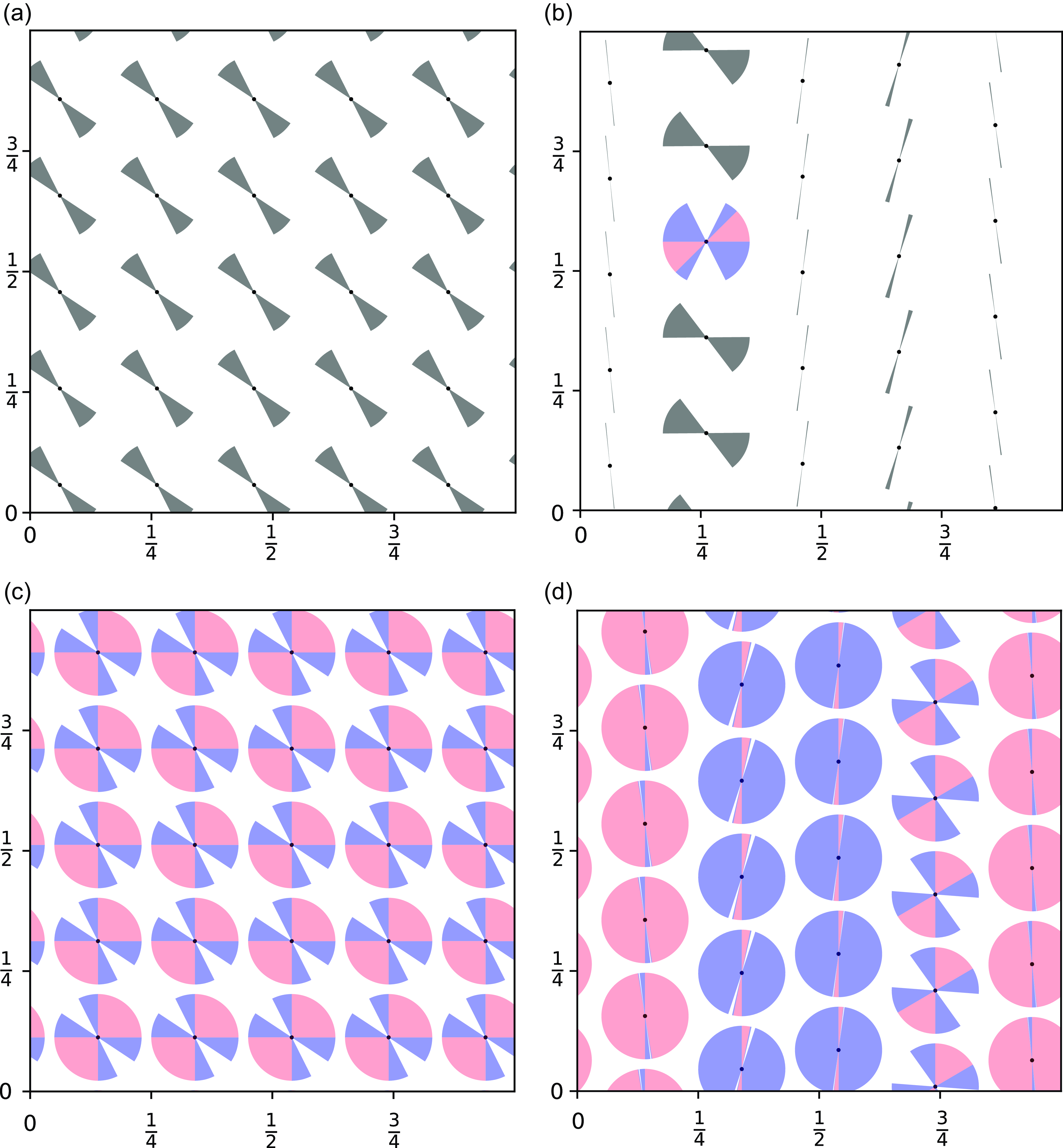
Panel (a) shows the
 $25$
pre-images of a randomly chosen point
 $x = (0.594, 0.287)$
under the map
 $E_k$
when
 $k=2$
, together with the cones
 $E_k^{-1} \Delta _\alpha ^v$
with
 $\alpha = 2$
. Panel (b) shows the pre-images of these points under the map
 $S_t^{-1} = S_{-t}$
for
 $t=1.5$
, together with the corresponding cones. (Taking a bigger
 $t$
would make some of the cones hard to see because they would be too thin.) In this example we see that
 $(Df_{y})^{-1} \Delta _\alpha ^v \subset \Delta _\alpha ^v$
for
 $20$
choices of
 $y \in f^{-1}(x)$
. At one of the points
 $y$
(say
 $y_0$
) for which this fails, the illustration shows the horizontal cone
 $\Delta _\alpha ^h$
instead of
 $(Df_{y_0})^{-1}\Delta _\alpha ^v$
. The horizontal cone at
 $y_0$
is divided into two parts, reflecting the quadrant to which it is mapped under
 $E^{-1}$
. The pre-images of this horizontal cone are shown in panel (c). Finally, in panel (d) we see
 $(Df_z)^{-1}\Delta _\alpha ^h$
for every
 $z \in f^{-1}(y_0)$
. For
 $10$
choices of
 $z$
, vectors in
 $\Delta _\alpha ^h$
which lie in the second and fourth quadrant get mapped into
 $\Delta _\alpha ^v$
while, for
 $10$
other choices, vectors in the first and third quadrant get mapped into
 $\Delta _\alpha ^v$
.

4. Continuity of the characteristic exponents
In this part we prove Theorem B. Recall that from Proposition 2.2 we already know that if
 $f\in \mathcal U_1$
then for
 $\mu$
-a.e. point
 $x\in \mathbb {T}^2$
(or
 $\hat {\mu }$
-a.e.
 $\hat {x}\in {\mathbf {L}_{f}}$
) the two Lyapunov exponents at
 $x$
(resp.
 $\hat {x}$
) are different.
Let us spell out some of the facts used in the proof. The first lemma is well known in the theory (cf. [Reference VianaVia14]).
Lemma 4.1 (Projectivized cocycles). Assume that
 $A$
is a two-dimensional cocycle over the invertible map
 $f:M\rightarrow M$
with invariant measure
 $\mu$
. Let
 ${\mathbb {P}} f:{\mathbb {P}} M\rightarrow {\mathbb {P}} M$
be its projectivization, which is a bundle map over
 $f$
. Assume that the two Lyapunov exponents
 $\lambda ^+(x)$
and
 $\lambda ^-(x)$
are different at
 $\mu$
-a.e. point, with the corresponding Lyapunov subspaces
 $E^+(x)$
and
 $E^-(x)$
. Then we have the following.
-
– If
$\mu$
is ergodic there are exactly two ergodic lifts of
$\mu$
to
$PM$
,
$\mu ^{p+}$
and
$\mu ^{p-}$
. The disintegrations of
$\mu ^{p+}$
along the fibers of
${\mathbb {P}} M$
are exactly the Dirac measures at the Lyapunov spaces
$E^+$
, and a similar statement holds for
$\mu ^{p-}$
. -
– Suppose that
$\mu ^p$
is a lift of
$\mu$
(not necessarily ergodic) to
${\mathbb {P}} M$
. Then there is a measurable
$f$
-invariant function
$\rho :M\rightarrow [0,1]$
such that the disintegrations of
$\mu ^p$
along the fibers of
${\mathbb {P}} M$
are
$\rho (x)\delta _{E^+(x)}+(1-\rho (x))\delta _{E^-(x)}$
.






4.1 Product measures
We will be concerned with measures which have product disintegrations. The following has a direct analog in the so-called ‘cocycles with continuous holonomy’, and ‘
 $s$
-states and
 $u$
-states’, in previous work. We state the results in the general case of products of metric spaces: the existence of holonomy translates in our setting to the product structure of the spaces involved, while the invariance of the disintegrations of measures under holonomies translates to the product structure of the corresponding measures.
The next result is a characterization of product measures. Let us note that what we call a ‘product measure’ is stronger than the notion of a ‘measure with product structure’ which is common in the literature; more precisely we ask that the density is constant, so the measure on the product space is exactly the product of two measures on the two factor spaces.
Lemma 4.2 (Product measures). Let
 $X$
,
 $Y$
be compact metric spaces and
 $\mu$
a Borel probability measure on
 $X\times Y$
. Then
 $\mu$
is a product measure (i.e.
 $\mu =(\pi _{X})_*\mu \times (\pi _{Y})_* \mu$
) if and only if, for any
 $f\in C(X,\mathbb R)$
and
 $g\in C(Y,\mathbb R)$
, we have
 \begin{align} \nonumber \int _{X\times Y}f\circ \pi _X \cdot g\circ \pi _Y \, d\mu &= \int _{X\times Y} f \circ \pi _X \, d\mu \int _{X\times Y } g \circ \pi _Y \, d\mu \\ & = \int _X f\ d(\pi _{X})_* \mu \cdot \int _Y g \, d(\pi _{Y})_* \mu . \end{align}
Proof.
The condition on the integrals is equivalent to the fact that any pair of measurable functions
 $f:(X,(\pi _{X})_*\mu ) \to {\mathbb {R}}$
and
 $g:(Y,(\pi _{Y})_* \mu ) \to {\mathbb {R}}$
are independent, and this is equivalent to
 $\mu$
being a product measure.
The next result says that the property of being a product measure is closed under weak* limits.
Corollary 4.1 (Limits of product measures). A weak* limit of Borel product probability measures is a Borel product probability measure.
Proof.
The proof is a direct application of Lemma 4.2, using the observation that if
 $(\mu ^k)_k$
converges weakly to
 $\mu$
then the same happens for its marginals on
 $X$
and
 $Y$
.
We are interested in the case when a measure has disintegrations which are product measures. For simplicity we consider products of metric spaces, but similar results can be obtained for continuous bundles. We first give a characterization of measures with product disintegrations.
Lemma 4.3 (Measures with product disintegrations). Let
 $X,Y,Z$
be compact metric spaces and let
 $\mu$
be a Borel probability measure on
 $W = X \times Y \times Z$
. Denote by
 $\mu _x$
the conditionals of
 $\mu$
along
 $\{x\} \times Y \times Z$
for
 $x\in X$
. Then
 $\mu _x$
is a product measure for
 $(\pi _{X})_*\mu$
-a.e.
 $x\in X$
if and only if, for every
 $f\in C(X,\mathbb R),\ g\in C(Y,\mathbb R)$
and
 $h\in C(Z,\mathbb R)$
, we have
 \begin{equation} \int _W f(x)\cdot g(y)\cdot h(z)\, d\mu (x,y,z)=\int _W \left (\int _Y g \, d(\pi _{Y})_* \mu _x\right )\cdot f(x) \cdot h(z)\, d\mu (x,y,z). \end{equation}
Proof.
Consider the probability kernel induced by
 $\{\mu _z:z\in X\}$
: that is, for
 $F\in C(Y \times Z, {\mathbb {R}})$
,
 $ KF(x)=\int _{Y \times Z} F(y,z)\, d\mu _x(y,z)$
. By the previous lemma,
 $\mu _x$
is a product if and only if for every
 $g \in C(Y,\mathbb R), h\in C(Z,\mathbb R)$
the following holds:
 \begin{equation*} K(gh)(x)=\int _Y g \, d(\pi _{Y})_* \mu _x \cdot \int _Z h \ d(\pi _{Z})_*\mu _x. \end{equation*}
Since continuous functions are separating in
 $L^1(X,(\pi _{X})_*\mu )$
, the previous equality holds for
 $(\pi _{X})_*\mu$
-a.e.
 $x\in X$
if and only if for every
 $f\in C(X,\mathbb R)$
the following holds:
 \begin{align} \int _X K(gh) \cdot f \ d(\pi _{X})_*\mu = \int _X f(x) \cdot \int _Y g \, d(\pi _{Y})_* \mu _x \cdot \int _Z h \ d(\pi _{Z})_*\mu _x \ d(\pi _X)_* \mu (x). \end{align}
But
 $\int _Z h \ d(\pi _Z)_* \mu _x = \int _{Y \times Z} h(z) \, d\mu _x(y,z)$
, so the right-hand side of (20) can be written as
 \begin{align*} &\int _X f(x) \cdot \left (\int _Y g \, d(\pi _{Y})_*\mu _x \int _{Y \times Z} h(z)\, d\mu _x(y, z)\right ) d(\pi _{X})_*\mu (x)\\ & \quad =\int _X f(x) \left (\int _{Y \times Z} \int _Y g(y') d(\pi _{Y})_*\mu _x(y')\cdot h(z) \, d\mu _x(y, z)\right )d(\pi _{X})_*\mu (x)\\ & \quad =\int _W \int _Y g \, d(\pi _{Y})_* \mu _x \cdot f(x) \cdot h(z) \, d\mu (x,y,z). \end{align*}
By the definition of conditionals,
 \begin{equation*}\int _P K(fg)(z) h(z)\,d\pi _{P*}\mu (z)=\int _X f(x)g(y)h(z)\,d\mu (x,y,z), \end{equation*}
and the claim follows.
We would like to pass to the limit the property of having product disintegrations. Unfortunately this is not always the case, and one can easily construct examples of a sequence of measures with product disintegrations which converges in the weak* topology to a measure without product disintegrations. We therefore have to add some extra conditions in order to be able to pass to the limit. We have the following result.
Lemma 4.4 (Limits of measures with product disintegrations). Let
 $X, Y, Z$
be compact metric spaces. Let
 $\mu ^k$
be a sequence of Borel probability measures on
 $W =X \times Y \times Z$
such that
 $\mu ^k$
converges to
 $\mu$
in the weak* topology, and for
 $(\pi _{X})_* \mu ^k$
-a.e.
 $x \in X$
, the disintegration
 $\mu _x^k$
is a product measure on
 $Y \times Z$
. Suppose that one of the following two conditions is verified.
-
(1) Given any
$g \in C(Y, {\mathbb {R}})$
, the functions
$\alpha ^k(x) = \int _Y g \, d(\pi _Y)_* \mu _x^k$
and
$\alpha (x) =$
$\int _Y g \, d(\pi _Y)_* \mu _x$
can be extended continuously to all of
$X$
and, moreover,
$\alpha ^k(x)$
converges uniformly to
$\alpha (x)$
. -
(2) The measures
$(\pi _{X})_* \mu ^k$
are equivalent to
$(\pi _{X})_* \mu$
with the Jacobian
$J^k= {d(\pi _{X})_* \mu ^k}/{d(\pi _{X})_* \mu }$
uniformly bounded from above, and
$(\pi _Y)_*\mu _x^k$
converges in the weak* topology to
$(\pi _Y)_*\mu _x$
for
$(\pi _{X})_*\mu$
-a.e.
$x\in X$
.









Then the disintegrations
 $\mu _x$
of
 $\mu$
are product measures for
 $(\pi _{X})_* \mu$
-a.e.
 $x\in X$
.
Proof.
Fix
 $f\in C(X,{\mathbb {R}}), g \in C(Y,{\mathbb {R}})$
and
 $h\in C(Z,{\mathbb {R}})$
. By Lemma 4.3 we have
 \begin{equation*} \int _W f(x)\cdot g(y)\cdot h(z)\, d\mu ^k(x,y,z)=\int _W \left (\int _Y g\, d(\pi _{Y})_*\mu _x^k \right )\cdot f(x) \cdot h(z) \, d\mu ^k(x,y,z). \end{equation*}
The left-hand side converges to
 $ \int _W f(x)\cdot g(y)\cdot h(z)\, d\mu (x,y,z)$
when
 $k$
goes to infinity and hence, by the same lemma, to prove the result it suffices to show that the right-hand side converges to
 $\int _W \left ( \int _Y g \, d(\pi _{Y})_*\mu _x\right )\cdot f(x)\cdot h(z)\, d\mu (x,y,z)$
.
Consider the functions
 $\alpha ^k, \alpha : X \rightarrow {\mathbb {R}}$
,
-
–
$\alpha ^k(x)=\int _Y g \, d(\pi _{Y})_* \mu _x^k$
and
$\alpha (x)=\int _Y g \, d(\pi _{Y})_* \mu _x$
,


which are defined for
 $(\pi _{X})_* \mu ^k\text{-} \text{ and } (\pi _{X})_* \mu $
-a.e.
 $x\in X$
, respectively, and
 $\beta ^k, \beta : W \to {\mathbb {R}}$
,
-
–
$\beta ^k(x,y,z)=\alpha ^k(x)\cdot f(x) \cdot h(z)$
and
$\beta (x,y,z)=\alpha (x)\cdot f(x) \cdot h(z)$
.


Then
 \begin{align*} \left |\int _W \beta ^k\, d\mu ^k-\int _W \beta \, d\mu \right |\leq &\left |\int _W \beta \, d\mu ^k-\int _W \beta \, d\mu \right |\\ &+|g|_{\infty }\cdot |h|_{\infty }\int _X |\alpha ^k-\alpha |\ d (\pi _X)_* \mu _k. \end{align*}
If condition (1) from the hypothesis is satisfied, then the functions
 $\alpha ^k$
are continuous and converge uniformly to
 $\alpha$
, and hence both terms above converge to zero. On the other hand, if condition (2) is satisfied, then there exists
 $X'\subset X$
with
 $(\pi _{X})_*\mu (X')=1$
such that, for
 $x\in X', \alpha ^k(x), \alpha (x)$
are well defined and
 $\lim _{k\to \infty }\alpha ^k(x)=\alpha (x)$
. Since
 $\alpha ^k,\alpha , J^k$
are uniformly bounded, we also get
 \begin{equation*} \lim _{k\rightarrow \infty }\int _X |\alpha -\alpha _k|\ d(\pi _{X})_* \mu ^k=\lim _{k\rightarrow \infty }\int _X |\alpha -\alpha _k|\cdot J^k \ d(\pi _{X})_* \mu =0. \end{equation*}
That
 $\left |\int _W \beta \, d\mu ^k-\int _W \beta \, d\mu \right |$
converges to
 $0$
as
 $k\to \infty$
can be seen as follows. Take
 $(\tilde \alpha _m)_m$
, a sequence of continuous functions converging in
 $L^1(\pi _{X\ast }\mu )$
to
 $\alpha$
and consider the corresponding
 $\tilde \beta ^m=\alpha ^m\cdot g\cdot h$
. Then
 \begin{align*} &\left |\int _W \beta \, d\mu ^k-\int _W \beta \, d\mu \right | \\ &\quad \leq \left |\int _W \beta -\tilde \beta ^m\, d\mu ^k\right |+\left |\int _W \tilde \beta ^m\, d\mu ^k-\tilde \beta ^m\, d\mu \right |+\left |\int _W \tilde \beta ^m-\beta \, d\mu \right |\\ &\quad \leq |g|_{\infty }\cdot |f|_{\infty }\cdot \left(\sup _k|J_k|_{\infty }+1\right)\int _X|\tilde \alpha ^m-\alpha |\ d\pi _{X\ast }\mu +\left |\int _W \tilde \beta ^m\, d\mu ^k-\tilde \beta ^m\, d\mu \right |. \end{align*}
For large
 $m$
the first term is arbitrarily small, and then we can take
 $k$
to be large so that the second term is also small. This concludes the proof.
Remark 4.1. The conditions of Lemma
4.4 in fact mean that one of the two factors of the product disintegrations (corresponding to M) converges weakly to the factor of the disintegrations of the limit measure (uniformly or pointwise). However the other factor of the disintegrations (corresponding to
 $N$
) may not converge.
4.2 Proof of continuity
Before digging into the proof of Theorem B, let us make a technical comment on it.
Let
 $(f_n)$
be a sequence in
 $\mathcal U_1$
converging to
 $f\in \mathcal U_1$
in the
 $\mathcal C^1$
topology. For each
 $n$
let
 ${\hat {\mu }}_n$
be the unique
 ${\hat {f}}_n$
-invariant measure on
 ${\mathbf {L}_{f}}[f_n]$
projecting on
 $\mu$
. By Proposition 2.2 we know that all these cocycles have different Lyapunov exponents at almost every point. Let
 $\hat {\mu }_n^{p-}$
be the lift of
 $\hat {\mu }_n$
to
 ${\mathbb {P}} \hat {f}_n$
such that the disintegrations of
 $\hat {\mu }_n^{p-}$
along the projective fibers are Dirac measures at the Lyapunov subspaces (
 $\delta _{E^-_n}$
) for
 $\hat {\mu }_n$
-a.e. point. Similarly, the corresponding objects for
 $f$
are
 ${\mathbf {L}_{f}},\ \hat {\mu },\ {\mathbb {P}}\hat {f}$
and
 $\hat {\mu }^{p-}$
.
Denoting by
 $v^s(x)$
the unit vector in the Lyapunov subspace
 $E^-(x)$
, we have
 \begin{align} \int _{\mathbb T^2}\chi ^-(f_n)\,d\mu =\int _{{\mathbf {L}_{f}}[f_n]}\chi ^-({\hat {f}}_n)\,d{\hat {\mu }}_n&=\int _{{\mathbf {L}_{f}}[f_n]}\log \|D(f_n)_{\hat {x}}v^s\|\,d{\hat {\mu }}_n(\hat {x})\nonumber\\ &=\int _{{\mathbb {P}} {\mathbf {L}_{f}}[f_n]}\log \|D(f_n)_{\hat {x}}v\|\,d{\hat {\mu }}_n^{p-}(\hat {x},v), \end{align}
and similarly for
 $f$
.
To prove the continuity of the negative Lyapunov exponent (which indeed implies the continuity of the positive Lyapunov exponent), we would like to pass the right-hand side of (21) to the limit, saying that
 ${\hat {\mu }}_n^{p-}$
converges to
 ${\hat {\mu }}^{p-}$
in the weak* topology. However, there’s a technical nuisance here: the space
 $\mathbf {L}_{f}$
depends on
 $f$
, so that the measures
 ${\hat {\mu }}_n$
live on different spaces. The same is true for the measures
 ${\hat {\mu }}_n^{p-}$
. For this reason, it is more convenient to work on an abstract solenoidal manifold
 $\operatorname {Sol}$
whose construction is outlined in Appendix A. Indeed, each
 ${\mathbf {L}_{f}}[f_n]$
is homeomorphic to
 $\operatorname {Sol}$
in a canonical fashion. Thus (21) may be rewritten as
 \begin{equation} \int _{\mathbb T^2}\chi ^-(f_n)\,d\mu =\int _{\operatorname {Sol}}\chi ^-(Sf_n)\,d{\boldsymbol {\mu }}_n= \int _{{\mathbb {P}} \operatorname {Sol}}\|D f_n({{\mathbf {x}}}) v\|\,d{\boldsymbol {\mu }}_n^{p-}({\mathbf {x}},v), \end{equation}
where
 ${\boldsymbol {\mu }}_n$
is the unique
 $Sf_n$
-invariant measure in
 $\operatorname {Sol}$
projecting on
 $\mu$
and
 ${\boldsymbol {\mu }}_n^{p-}$
is the corresponding stable measure on
 $P Sf_n$
.
Remark 4.2. We could dispense with
 $\mathbf {L}_{f}$
altogether and replace it with
 $\operatorname {Sol}$
throughout this paper. Indeed,
 $\mathbf {L}_{f}$
can be seen simply as an embedding of
 $\operatorname {Sol}$
into
 $(\mathbb {T}^2)^{\mathbb {Z}+}$
with the disadvantages that it depends on
 $f$
and that its solenoidal structure is somewhat hidden. However, we have decided to stick to
 $\mathbf {L}_{f}$
in all sections except this one, because it is more familiar. We hope that this helps the casual reader.
Proof of Theorem B. Let
 $(f_n)$
be a sequence in
 $\mathcal U_1$
converging to
 $f\in \mathcal U_1$
in the
 $\mathcal C^1$
topology, and let
 ${\boldsymbol {\mu }}_n$
and
 ${\boldsymbol {\mu }}_n^{p-}$
be the lifts to
 $\operatorname {Sol}$
and
 ${\mathbb {P}} \operatorname {Sol}$
as above. By virtue of (22), to prove Theorem B it suffices to prove that
 ${\boldsymbol {\mu }}_n^{p-}$
converges weakly* to
 ${\boldsymbol {\mu }}^{p-}$
as
 $n \to \infty$
. By Proposition A.5, this is equivalent to saying that
 $\tilde {{\boldsymbol {\mu }}}_n^{p-}$
converges weakly* to
 $\tilde {{\boldsymbol {\mu }}}^{p-}$
, where
 $\tilde {{\boldsymbol {\mu }}}_n^{p-}$
and
 $\tilde {{\boldsymbol {\mu }}}^{p-}$
are, respectively, the lifts of
 ${\boldsymbol {\mu }}_n^{p-}$
and
 ${\boldsymbol {\mu }}^{p-}$
to
 ${\mathbb {P}} ({\mathbb {R}^2} \times \Sigma )$
.Footnote
5
Suppose, for the purposes of contradiction, that
 ${\boldsymbol {\mu }}_n^{p-}$
converges to some
 ${\boldsymbol {\mu }}^p$
different from
 ${\boldsymbol {\mu }}^{p-}$
. We are going to show that
 ${\boldsymbol {\mu }}^p$
has product disintegrations, that is, that it can be written as
 \begin{equation} {\boldsymbol {\mu }}^p = \int _{\mathbb {T}^2} {\boldsymbol {\mu }}_x \times \nu _x \, d\mu (x) \end{equation}
for some (measurable) family of measures
 $\nu _x$
on
 ${\mathbb {P}} {\mathbb {R}^2}$
. To do this, we have to analyze the convergence of
 ${\boldsymbol {\mu }}_n^{p-}$
to
 ${\boldsymbol {\mu }}^p$
in more detail, but instead of analyzing this convergence directly, we analyze the convergence of a sequence of measures on
 $[0,1]^2 \times \Sigma \times {\mathbb {P}} {\mathbb {R}^2}$
which mirrors this sequence. The advantage of this is that the underlying space is then a product space, allowing us to apply Lemma 4.4.
Let us write
 \begin{equation*} \begin{array}{lll} Q = [0,1]^2, & \quad \tilde {\boldsymbol {\eta }}_n = \tilde {{\boldsymbol {\mu }}}_n \vert Q \times \Sigma , & \quad \tilde {\boldsymbol {\eta }}_n^{p-} = \tilde {{\boldsymbol {\mu }}}_n^{p-} \vert Q \times \Sigma \times {\mathbb {P}} {\mathbb {R}^2}, \\ \tilde {\eta } = \tilde {\mu } \vert Q, & \tilde {\boldsymbol {\eta }} = \tilde {{\boldsymbol {\mu }}} \vert Q \times \Sigma , & \tilde {\boldsymbol {\eta }}^{p} = \tilde {{\boldsymbol {\mu }}}^{p} \vert Q \times \Sigma \times {\mathbb {P}} {\mathbb {R}^2}. \end{array} \end{equation*}
Note that the boundary of
 $Q \times \Sigma \times {\mathbb {P}} {\mathbb {R}^2}$
has zero
 $\tilde {{\boldsymbol {\mu }}}^{p}$
-measure,
 $(\pi _G,i)_* \tilde {\boldsymbol {\eta }}_n^{p-} = {\boldsymbol {\mu }}_n^{p-}$
, and
 $(\pi _G,i)_* \tilde {\boldsymbol {\eta }}^p = {\boldsymbol {\mu }}^p$
. (See Appendix A for notation.) We are now in the following situation.
-
(1) The projection of
$\tilde {\boldsymbol {\eta }}_n^{p-}$
to
$Q \times \Sigma$
is
$\tilde {\boldsymbol {\eta }}_n$
. The disintegrations of
$\tilde {\boldsymbol {\eta }}_n^{p-}$
along
$ \{(\tilde {x}, \boldsymbol {\omega }) \} \times {\mathbb {P}} {\mathbb {R}^2}$
are
$\delta _{E^-_n(\pi _{\mathrm {cov}}(\tilde {x}))}$
(see Lemma 4.1). -
(2) The projection of
$\tilde {\boldsymbol {\eta }}_n$
to
$Q$
is
$\tilde {\eta }$
(the restriction of Lebesgue to the unit square). The disintegrations of
$\tilde {\boldsymbol {\eta }}_n$
along
$\{\tilde {x}\}\times \Sigma$
are
$\tilde {{\boldsymbol {\mu }}}_{n,\tilde {x}}$
(defined as in (39)). -
(3) The projection of
$\tilde {\boldsymbol {\eta }}_n^{p-}$
to
$Q$
is also
$\tilde {\eta }$
. The disintegrations of
$\tilde {\boldsymbol {\eta }}_n^{p-}$
along
$\{\tilde {x}\} \times \Sigma \times {\mathbb {P}} {\mathbb {R}^2}$
are
$\delta _{E^-_n(\pi _{\mathrm {cov}}(\tilde {x}))}\times \tilde {{\boldsymbol {\mu }}}_{n,\tilde {x}}$
. (This is because
$E^-_n$
is constant on the fibers.) -
(4) The disintegrations
$\tilde {{\boldsymbol {\mu }}}_{n,\tilde {x}}$
vary continuously with respect to
$\tilde {x}\in Q$
. Furthermore
$\tilde {{\boldsymbol {\mu }}}_{n,\tilde {x}}$
converge (uniformly) to
$\tilde {{\boldsymbol {\mu }}}_x$
(see Remark 4.1 and Proposition A.4).









All these considerations show that we are within the hypotheses of Lemma 4.4, with
 $Q$
in place of
 $X$
,
 $\Sigma$
in place of
 $Y$
,
 ${\mathbb {P}} {\mathbb {R}^2}$
in place of
 $Z$
,
 $\tilde {\boldsymbol {\eta }}_k^{p-}$
in place of
 $\mu ^k$
, and
 $\tilde {\boldsymbol {\eta }}^{p}$
in place of
 $\mu$
. (In fact, both condition (1) and condition (2) are satisfied.) As a consequence, we have that
 \begin{equation} \tilde {\boldsymbol {\eta }}^p=\int _{ Q} \tilde {{\boldsymbol {\mu }}}_{\tilde {x}} \times \tilde {\nu }_{\tilde {x}} \ d\tilde {\eta }, \end{equation}
where
 $\tilde {\nu }_{\tilde {x}}$
,
 $\tilde {x} \in Q$
, are measures on
 ${\mathbb {P}} {\mathbb {R}^2}$
(depending measurably on
 $x$
). Writing
 $\nu _x = \tilde {\nu }_{\tilde {x}}$
when
 $\pi _{\mathrm {cov}}(\tilde {x}) = x$
(which is well-defined
 $\tilde {\eta }$
-almost everywhere) and applying
 $(\pi _G,i)^*$
to both sides of (24) gives (23).
For the remainder of the proof we will abandon the space
 $\operatorname {Sol}$
in favor of
 $\mathbf {L}_{f}$
and apply Lemma 4.1. Thus, writing
 ${\hat {\mu }}^p = (\phi ,i)_* {\boldsymbol {\mu }}^p$
and applying
 $(\phi ,i)_*$
to both sides of (23) we see that
 \begin{equation*} {\hat {\mu }}^p = \int _{\mathbb {T}^2} \hat {\mu }_x \times \nu _x \, d\mu (x). \end{equation*}
Since
 ${\boldsymbol {\mu }}_n^p$
are invariant under
 $PS f_n$
, and
 $PS f_n$
converges to
 $PS f$
, we have that
 ${\boldsymbol {\mu }}^p$
is invariant under
 $PS f$
. Consequently,
 ${\hat {\mu }}^p$
is invariant under
 $P {\hat {f}}$
. Lemma 4.1 tells us that there exists an
 $\hat {f}$
-invariant function
 $\hat {\rho }:{\mathbf {L}_{f}}\rightarrow [0,1]$
such that
 \begin{equation*} \hat {\mu }^p=\int _{{\mathbf {L}_{f}}}\hat {\rho }\delta _{E^+}+(1-\hat {\rho })\delta _{E^-}\ d\hat {\mu }. \end{equation*}
Since the ergodic components of
 $\hat {f}$
are exactly the pre-images under
 $\pi _{\mathrm{ext}}$
of the ergodic components of
 $f$
, we have in fact that
 $\hat {\rho }$
is constant on the fibers
 $\pi _{\mathrm{ext}}^{-1}(x)$
. In other words, there exists a measurable
 $f$
-invariant function
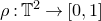 $\rho :\mathbb T^2\rightarrow [0,1]$
such that
 $\hat {\rho }=\rho \circ \pi _{\mathrm{ext}}$
. Remembering that
 $E^-$
is also constant on the fibers, we have that
 \begin{eqnarray*} \int _{{\mathbf {L}_{f}}}\rho \circ \pi _{\mathrm{ext}}\delta _{E^+}\,d\hat {\mu }&=&\hat {\mu }^p-\int _{{\mathbf {L}_{f}}}(1-\rho \circ \pi _{\mathrm{ext}})\delta _{E^-}\,d\hat {\mu }\\ &=&\int _{\mathbb T^2}\nu _x\times {\hat {\mu }}_x\,d\mu -\int _{\mathbb T^2}(1-\rho )\delta _{E^-}\times {\hat {\mu }}_x\,d\mu \\ &=&\int _{\mathbb T^2}\left (\nu _x-(1-\rho )\delta _{E^-}\right )\times {\hat {\mu }}_x\,d\mu \\ &=&\int _{{\mathbf {L}_{f}}}\nu _{\pi _{\mathrm{ext}}(\hat {x})}-(1-\rho \circ \pi _{\mathrm{ext}})\delta _{E^-}\,d\hat {\mu }. \end{eqnarray*}
Then for
 $\hat {\mu }$
-a.e.
 $\hat {x}$
we have that
 \begin{equation*}\rho (\pi _{\mathrm{ext}}(\hat {x}))\delta _{E^+(\hat {x})}=\nu _{\pi _{\mathrm{ext}}(\hat {x})}-(1-\rho (\pi _{\mathrm{ext}}(\hat {x})))\delta _{E^-(\hat {x})}. \end{equation*}
If
 $\hat {\mu }^p$
is different from
 $\hat {\mu }^{p-}$
then
 $\rho$
is nonzero on a set of positive measure. Then there exists a set of points of positive
 $\mu$
-measure
 $x\in \mathbb T^2$
such that
 $\rho (x)\gt 0$
and
 $\rho (x)\delta _{E^+(\hat {x})}=\nu _{x}-(1-\rho (x))\delta _{E^-(\hat {x})}$
holds for
 ${\hat {\mu }}_x$
-a.e
 $\hat {x}\in \pi _{\mathrm{ext}}^{-1}(x)$
. Since the right-hand side depends only on
 $x$
, we have that, for
 ${\hat {\mu }}_x$
-a.e.
 $\hat {x}$
, the unit vector
 $v^+(\hat {x})$
inside
 $E^+(\hat {x})$
is constant, equal to say
 $v^+(x)$
. Since almost every
 $x\in \mathbb {T}^2$
has the property that
 ${\hat {\mu }}_x$
-a.e. point is Lyapunov regular, then there exists a set
 $A\subset \mathbb {T}^2$
of positive
 $\mu$
-measure such that for every
 $x\in A$
we have
 \begin{eqnarray*} \lim _{n\rightarrow \infty }\frac {I(x,v^+;f^n)}n&=&\lim _{n\rightarrow \infty }\frac 1n\int _{\pi _{\mathrm{ext}}^{-1}(x)}\log \|(D_{\hat {x}}\hat {f})^{-n}(v^+)\|\,d{\hat {\mu }}_x\\ &=&\int _{\pi _{\mathrm{ext}}^{-1}(x)}\lim _{n\rightarrow \infty }\frac 1n\log \|(D_{\hat {x}}\hat {f})^{-n}(v^+)\|\,d{\hat {\mu }}_x\\ &=&\int _{\pi _{\mathrm{ext}}^{-1}(x)}-\chi ^+\,d{\hat {\mu }}_x. \end{eqnarray*}
This implies that for
 $\mu$
-a.e.
 $x\in A$
we have
 \begin{equation*}\chi ^+(x)=-\lim _{n\rightarrow \infty }\frac {I(x,v^+;f^n)}n\leq -C_{\chi }(f).\end{equation*}
But, on the other hand, we know from Proposition 2.2 that for
 $\mu$
-a.e.
 $x\in \mathbb {T}^2$
we have
 \begin{equation*} \chi ^-(x)\leq -C_{\chi }(f), \end{equation*}
so for
 $\mu$
-a.e.
 $x\in A$
we have
 \begin{equation*} -2C_{\chi }(f)\geq \chi ^+(x)+\chi ^-(x)=\lim _{n\rightarrow \infty }\log (\det Df^n(x))\geq C_{\det }(f), \end{equation*}
which is a contradiction of the definition of
 $\mathcal U_1$
. This finishes the proof.
5. Pesin theory for endomorphisms
Here we collect some facts about non-uniformly hyperbolic endomorphisms that will be used in the forthcoming section to prove (stable) ergodicity. Throughout this part
 $f:M\to M$
denotes an endomorphism of the compact surface
 $M$
; the distance on
 $M$
(induced by a Riemannian metric) between
 $x,y\in M$
is denoted by
 $d(x,y)$
. It is assumed that
 $f$
is non-uniformly hyperbolic with respect to a smooth area
 $\mu$
, and we maintain the notation
 ${\mathbf {L}_{f}}, {\hat {f}},{\hat {\mu }}$
, etc. as before (see § 2.1). We point out that in our notation
 $x_n$
(and not
 $x_{-n}$
) is a pre-image of
 $x_0$
for
 $f^n$
. Recall also the definition of the set of regular points
 $\mathcal {R}$
(cf.
 $\hat {\mathcal {R}}$
) given in Lemma 2.1. We will use the following definitions of [Reference LiuLiu08] and [Reference Qian and ZhuQZ02].
Definition 5.1. Let
 $\hat {x}\in \hat {\mathcal {R}}, x=\pi _{\mathrm {ext}}(\hat {x})$
.
-
(1) A
$\mathcal C^{1,1}$
embedded interval
$W^{u}_{\mathrm {loc}}(\hat {x}) \subset M$
is a local unstable manifold at
$\hat {x}$
if there exist constants
$\lambda \gt 0, 0\lt \varepsilon \lt {\lambda }/{200}, 0\lt C_1\leq 1\lt C_2$
such that
$y_0\in W^{u}_{\mathrm {loc}}(\hat {x})$
if and only if there exists a unique
${\hat {y}}\in {\mathbf {L}_{f}}, y_0=\pi _{\mathrm {ext}}(\hat {y})$
satisfying, for every
$n\geq 0$
,(25)
\begin{align} d(x_n,y_n)\leq C_1 e^{-n\varepsilon }, \end{align}
(26)
\begin{align} d(x_n,y_n)\leq C_2 e^{-n\lambda }. \end{align}
The lift of
$W^{u}_{\mathrm {loc}}(\hat {x})$
to
$\mathbf {L}_{f}$
using
$\pi _{\mathrm {ext}}$
is denoted by
$\hat {W}^{u}_{\mathrm {loc}}(\hat {x})$
. -
(2) The unstable manifold of
$f$
at
$\hat {x}$
isThe lift of
\begin{equation*} W^u(\hat {x})=\left\{y_0=\pi _{\mathrm {ext}}({\hat {y}}):\limsup _{n\to \infty }\frac {1}{n}\log d(x_n,y_n)\lt 0\right\}. \end{equation*}
$W^u(\hat {x})$
to
$\mathbf {L}_{f}$
using
$\pi _{\mathrm {ext}}$
is denoted by
$\hat{W}^u(\hat {x})$
.
-
(3) A
$\mathcal C^{1,1}$
embedded interval
$W^{s}_{\mathrm {loc}}(x) \subset M$
is a local stable manifold at
$x$
if there exist constants
$\lambda \gt 0, 0\lt \varepsilon \lt {\lambda }/{200}, 0\lt C_1\leq 1\lt C_2$
such that
$y\in W^{s}_{\mathrm {loc}}(x)$
if and only if, for every
$n\geq 0$
,(27)
\begin{align} d(f^n(x),f^n(y))\leq C_1 e^{-n\varepsilon }, \end{align}
(28)
\begin{align} d(f^n(x),f^n(y))\leq C_2 e^{-n\lambda }. \end{align}
The lift of
$W^{s}_{\mathrm {loc}}(x)$
to
$\mathbf {L}_{f}$
using
$\pi _{\mathrm {ext}}$
is denoted by
$\hat {W}^{s}_{\mathrm {loc}}(\hat {x})$
. -
(4) The stable manifold of
$f$
at
$x$
is
\begin{equation*} W^s(x)=\pi _{\mathrm {ext}}\bigg(\bigcup _{n=0}^{\infty } {\hat {f}}^{-n}\hat {W}^{s}_{\mathrm {loc}}({\hat {f}}^n \hat {x})\bigg). \end{equation*}







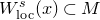




Remark 5.1. Observe that
 \begin{equation*} W^s(x) \subset \left\{y: \limsup \frac {1}{n}d(f^nx,f^ny)\lt 0\right\}=\bigcup _{k=0}^{\infty } f^{-k}(f^kW^s(x)). \end{equation*}
We record the following basic properties of stable and unstable manifolds.
Theorem 5.1 [Reference Qian and ZhuQZ02, Proposition 2.3]. There exists an increasing countable family
 $\{\hat {\Lambda }_k\}_{k\geq 0}$
of subsets of
 $\hat {\mathcal {R}}$
satisfying
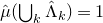 ${\hat {\mu }}(\bigcup _k \hat {\Lambda }_k)=1$
and such that we have the following.
-
(1) For every
$k$
there exists a continuous family of local unstable manifolds
$\{W^{u}_{\mathrm {loc}}(\hat {x}):\hat {x}\in \hat {\Lambda }_k\}$
such that, for every
$\hat {x}\in \hat {\Lambda }_k$
:-
(a)
$T_{x_0}W^{u}_{\mathrm {loc}}(\hat {x})=E^{+}(\hat {x})$
and, in particular,
$E^{+}(\hat {x})$
depends continuously on
$\hat {x}\in \hat {\Lambda }_k$
; -
(b) there exists a sequence of
$\mathcal C^{1,1}$
intervals
$\{W^u(\hat {x},-n)\}_{n\geq 0}$
in
$M$
with
-
–
$W^u(\hat {x},0)=W^{u}_{\mathrm {loc}}(\hat {x})$
, -
–
$fW^u(\hat {x},-n)\supset W^u(\hat {x},-n+1), \forall n\geq 1$
, -
–
$W^u(\hat {x})=\bigcup _{n\geq 0} f^nW^u(\hat {x},-n)$
.
-
-
-
(2) If
$\Lambda _k=\pi _{\mathrm {ext}}(\hat {\Lambda }_k)$
, then:
-
for every
$k$
there exists a continuous family of local stable manifolds
$\{W^{s}_{\mathrm {loc}}(x):x\in \Lambda _k\}$
such that, for every
$x\in \Lambda _k$
:-
–
$T_{x}W^{s}_{\mathrm {loc}}(x)=E^{-}(x)$
and, in particular,
$E^{-}(x)$
depends continuously on
$x\in \Lambda _k$
, -
–
$fW^{s}_{\mathrm {loc}}(x) \subset W^{s}_{\mathrm {loc}}(fx)$
.
-
-

















Proof. See [Reference Qian and ZhuQZ02, Proposition 2.3] and [Reference LiuLiu08].
Definition 5.2. The sets
 $\Lambda _k, \hat {\Lambda }_k$
above will be referred to as Pesin blocks.
It follows, in particular, that
 $W^{u}_{\mathrm {loc}}(\hat {x})$
has diameter uniformly bounded from below, for points in the same
 $\hat {\Lambda }_k$
, while the local stable manifolds have sizes uniformly bounded from below, for points in the same
 $\Lambda _k$
. Also,
 $fW^{s}_{\mathrm {loc}}(x)\subset W^{s}_{\mathrm {loc}}(fx)$
; it follows that
 $W^s(x)$
is an immersed submanifold of
 $M$
, and moreover that these manifolds
 $W^s$
(or
 $\hat {W}^s$
) form an invariant lamination of
 $M$
(respectively, of
 $\mathbf {L}_{f}$
). The global unstable manifolds
 $W^u$
do not form a lamination of
 $M$
(they may intersect), but the
 $\hat {W}^u$
do form an invariant lamination of
 $\mathbf {L}_{f}$
.
We will also need the following two results.
Proposition 5.1 (See [Reference LiuLiu08]). The stable lamination
 $W^s$
is absolutely continuous in the following sense. Given any Pesin block
 $\Lambda _k$
, the holonomy of local stable manifolds of points in
 $\Lambda _k$
between any two transversals is absolutely continuous (with respect to the Lebesgue measure of the two transversals). As a consequence, given any partition of
 $\mathbb {T}^2$
subordinated to the stable lamination, the disintegration of the Lebesgue measure on
 $\mathbb {T}^2$
along the elements of the partition is absolutely continuous with respect to the Lebesgue measure on stable manifolds.
Proposition 5.2 (See [Reference Liu and ShuLS11]). The unstable lamination
 $\hat {W}^u$
is absolutely continuous in the following sense. Given any partition of
 $\mathbf {L}_{f}$
subordinated to the Pesin unstable lamination
 $\hat {W}^u$
, the disintegrations
 $\hat {\mu }$
along the elements of the partition are absolutely continuous with respect to the Lebesgue measure on the unstable manifolds.
Here the Lebesgue measure on
 $\hat {W}^u(\hat {x})$
is given by the Lebesgue measure on
 $W^u(\hat {x})$
, since
 $\pi _{\mathrm {ext}}$
is a local homeomorphism between the two unstable manifolds.
6. Stable ergodicity
6.1 Large stable manifolds
The goal of this subsection is to prove that almost every (Lyapunov regular) point for the examples constructed in § 3 has a large stable manifold, in terms of diameter. We keep the notation from that section:
 $f_t=h_t\circ E, \delta \lt 1/{10}, \mathcal G, \alpha \gt 1, \Delta _{\alpha }^{v,h}, 0\lt a\lt b, e_v$
and
 $e_h$
.
If
 $\gamma :I\subset \mathbb R\rightarrow \mathbb {T}^2$
is a
 $\mathcal C^1$
curve, then
 $l(\gamma )$
is its (euclidean) length. Since in § 3 we used the maximum norm for the estimates, we will also consider the length of the curve in the maximum norm:
 \begin{equation*} l_m(\gamma ):=\int _I\max \{|\gamma _1'(t)|,|\gamma _2'(t)|\}\,dt. \end{equation*}
We clearly have
 $l_m(\gamma )\leq l(\gamma )\leq \sqrt 2l_m(\gamma )$
.
Let
 $l= {\alpha }/{5e_v}$
.
Definition 6.1. A
 $v$
-segment is a
 $\mathcal C^1$
curve on
 $\mathbb {T}^2$
which is a tangent to the vertical cone
 $\Delta _{\alpha }^v$
and whose length in the maximum norm is equal to
 $l$
.
Remark 6.1. Since
 $\alpha \gt 1$
, if
 $\gamma$
is a
 $v$
-segment then in fact the length of the projection of
 $\gamma$
on the vertical axis is
 $l$
.
Lemma 6.1.
Assume that
 $t\gt \max \{{2\alpha }/a, ({4\alpha ^2+\alpha e_v})/{e_va}\}$
. There exists
 $\mathcal U_2$
, a
 $\mathcal C^1$
open neighborhood of
 $f_t$
, such that any
 $f\in\mathcal U_2$
satisfies the following property: if
 $\gamma$
is a curve in
 $\mathbb {T}^2$
such that
 $f(\gamma )$
is a
 $v$
-segment, then
 $\gamma$
contains a
 $v$
-segment.
In other words, any pre-image of a
 $v$
-segment contains a
 $v$
-segment.
Proof. From § 3 we have the following.
-
(1) Action of
$E^{-1}$
:
$E^{-1}\Delta _{\alpha }^v\subset \Delta _{\alpha }^h$
and
$\mathrm {m} (E^{-1}|_{\Delta _{\alpha }^v})=e_v$
(
$E^{-1}$
takes
$\Delta _{\alpha }^v$
strictly inside
$\Delta _{\alpha }^h$
, expanding by more than
$e_v$
); -
(2) Action of
$Dh_t^{-1}$
: if
$t\gt {2\alpha }/a$
then for any
$x\in \overline {\mathcal G}$
we have
$D_xh_t^{-1}\Delta _{\alpha }^h\subset \overline {D_xh_t^{-1}\Delta _{\alpha }^h}\subset \Delta _{\alpha }^v$
and
$\mathrm {m}(D_xh_t^{-1}|_{\Delta _{\alpha }^h})\gt ({at-\alpha })/{\alpha }$
(
$D_xh_t^{-1}$
takes
$\Delta _{\alpha }^h$
strictly inside
$\Delta _{\alpha }^v$
, expanding by strictly more than
$({at-\alpha })/{\alpha }$
).









The second property is clearly
 $\mathcal C^1$
open, so we choose
 \begin{align*} \mathcal U_2:=&\{f=h\circ E:\ h \hbox { is a }\mathcal C^1\hbox { diffeomorphism of }\mathbb {T}^2\hbox { satisfying the above}\\ &\; \hbox { property 2}\}. \end{align*}
Let
 $\gamma$
be a curve in
 $\mathbb R^2$
such that
 $f(\gamma )$
is a
 $v$
-segment. Then
 $h(\gamma )$
is a pre-image of
 $f(\gamma )$
under some inverse branch of
 $E$
, so it is a curve inside the horizontal cone
 $\Delta _{\alpha }^h$
such that
 $l_m(h(\gamma ))\geq e_vl= {\alpha }/5$
. Since
 $h(\gamma )$
is inside
 $\Delta _{\alpha }^h$
we obtain that
 $l(\pi _1h(\gamma ))\geq 1/5$
(the length of the projection of
 $h(\gamma )$
on the horizontal direction is at least
 $1/5$
).
Recall that the critical intervals
 $I_1$
and
 $I_3$
have sizes
 $2\delta \lt 1/{2\tau _2}\leq 1/{10}$
, which implies that there exists a piece
 $\gamma _1$
inside
 $h(\gamma )$
which is inside
 $\mathcal G$
and has the length of the projection on the horizontal direction strictly greater than
 $1/{20}$
. Then our hypothesis implies that
 $h^{-1}(\gamma _1)$
will be inside the vertical cone
 $\Delta _{\alpha }^v$
and
 $l_m(h^{-1}(\gamma _1))\geq ({at-\alpha })/{20\alpha }$
. Since
 $t\gt ({4\alpha ^2+\alpha e_v})/{e_va}$
, we obtain that
 $l_m(h^{-1}(\gamma _1))\geq {\alpha }/{5e_v}=l$
, so
 $h^{-1}(\gamma _1)\subset \gamma$
contains a
 $v$
-segment.
Lemma 6.2.
Assume that
 $t\gt \max \{{2\alpha }/a,({4\alpha ^2+\alpha e_v})/{e_va}\}$
. There exists
 $\mathcal U_3\subset \mathcal U_2$
, a
 $\mathcal C^1$
open neighborhood of
 $f_t$
, such that any
 $f\in \mathcal U_3$
satisfies the following property: for any
 $x\in \mathbb {T}^2$
and any
 $\mathcal C^1$
curve
 $\gamma$
passing through
 $x$
, there exist
 $n\in \mathbb {N}$
,
 $y\in \mathbb {T}^2$
and a
 $v$
-segment
 $\gamma '$
passing through
 $y$
such that
 $f^n(y)=x$
and
 $f^n(\gamma ')=\gamma$
(some pre-image of
 $\gamma$
contains a
 $v$
-segment).
Proof.
We recall that Lemma 3.3 tells us that
 $f_t$
satisfies the following two properties:
-
(1) for any
$(x,v)\in T\mathbb {T}^2$
, there exists a pre-image
$(y,w)\in \mathcal G\times \Delta _{\alpha }^v$
; -
(2) for any
$x\in \mathbb {T}^2$
, there exists a pre-image
$y\in \mathcal G$
such that
$d(y,\mathcal C)\gt 1/{10}$
.





These are clearly
 $\mathcal C^1$
open properties, so we choose
 $\mathcal U_3\subset \mathcal U_2$
such that every
 $f\in \mathcal U_3$
satisfies them.
Let
 $x\in \mathbb {T}^2$
and
 $\gamma$
be a
 $\mathcal C^1$
curve passing through
 $x$
, and let
 $v$
be the vector tangent to
 $\gamma$
in
 $x$
. There exists a pre-image
 $x_1$
of
 $x$
such that
 $v_1=(D_{x_1}f_t)^{-1}v\in \Delta _{\alpha }^v$
and
 $x_1\in \mathcal G$
. Furthermore we can construct inductively a sequence of pre-images
 $(x_n)_{n\in \mathbb N}$
of
 $x$
such that:
-
(1)
$f(x_{n+1})=x_n$
,
$f^n(x_n)=x$
; -
(2)
$x_n\in \mathcal G$
,
$d(x_n,\mathcal C)\gt 1/{10}$
, for all
$n\geq 2$
.





Let
 $\gamma '_1$
be the pre-image of
 $\gamma$
passing through
 $x_1$
. Since the vector tangent to
 $\gamma '_1$
in
 $x_1\in \mathcal G$
is
 $v_1\in \Delta _{\alpha }^v$
, and
 $\gamma '_1$
is
 $\mathcal C^1$
, we can find a curve
 $\gamma _1$
inside
 $\gamma '_1$
which contains
 $x_1$
, is tangent to the vertical cone
 $\Delta _{\alpha }^v$
and is inside
 $\mathcal G$
. Taking the corresponding pre-images of
 $\gamma _1$
we obtain a sequence of curves
 $\gamma _n$
.
If all
 $\gamma _n$
stay inside
 $\mathcal G$
, then they will stay tangent to the vertical cone and will grow exponentially, so we eventually obtain a
 $v$
-segment.
If not, there exists
 $n\in \mathbb N$
such that
 $\gamma _{n+1}$
is not in
 $\mathcal G$
and
 $\gamma _n=f(\gamma _{n+1})$
is in
 $\mathcal G$
. But this implies that the length of the horizontal projection of the part of
 $\gamma _{n+1}$
inside
 $\mathcal G$
is greater than
 $1/{10}$
, and the considerations from the previous lemma imply that
 $\gamma _{n+1}$
must contain a
 $v$
-segment. This finishes the proof.
Let us now consider
 $f\in \mathcal U\cap \mathcal U_3$
, so
 $f$
is
 $\mathcal C^{1+\epsilon }$
, preserves the area and is non-uniformly hyperbolic. Let
 $A=\{x\in \mathbb {T}^2:\ W^s(x) \text { contains a } v\hbox{-}\text {segment}\}$
. The two previous lemmas show that:
-
–
$f^{-1}(A)\subset A$
; -
–
$\bigcup _{n=0}^{\infty }f^n(A)$
has full Lebesgue measure.


The next lemma says that a set with these properties has full measure.
Lemma 6.3.
Assume that
 $f$
preserves the probability measure
 $\mu$
, and the set
 $A$
satisfies
 $f^{-1}(A)\subset A$
and
 $\mu (\bigcup _{n=0}^{\infty }f^n(A))=1$
. Then
 $A$
has full
 $\mu$
-measure.
Proof.
Observe that the second condition implies that
 $A$
has positive measure.
Let
 $B\subset A$
be the set of recurrent points,
 $B=\{x\in A:\ \forall n\in \mathbb {N},\ \exists m\in \mathbb {N}, m\gt n, f^m(x)\in A\}$
. Then
 $\mu (B)=\mu (A)$
, and therefore
 $\bigcup _{n=0}^{\infty }f^n(B)$
has full measure.
We claim that
 $\bigcup _{n=0}^{\infty }f^n(B)\subset A$
. Let
 $x\in \bigcup _{n=0}^{\infty }f^n(B)$
. Then there exists
 $n\in \mathbb {N}$
such that
 $f^n(x)\in A$
, and therefore the first property gives us that
 $x\in A$
. This finishes the proof.
Putting the three lemmas above together we obtain the following proposition.
Proposition 6.1.
For any
 $t\gt \max \{{2\alpha }/a, ({4\alpha ^2+\alpha e_v})/{e_va}\}$
there exists a
 $\mathcal C^1$
open set of area-preserving non-uniformly hyperbolic endomorphisms
 $\mathcal U_3\cap \mathcal U$
containing
 $f_t$
such that any
 $f\in \mathcal U_3\cap \mathcal U$
of class
 $C^{1+\epsilon }$
satisfies the following property: Lebesgue almost every point
 $x\in \mathbb {T}^2$
has a large stable manifold, in the sense that
 $W^s(x)$
contains a
 $v$
-segment.
6.2 Local ergodicity
In this subsection we prove a general result from which both Theorems C and D can be deduced.
Proposition 6.2.
Let
 $f:\mathbb {T}^2 \to \mathbb {T}^2$
be a conservative non-uniformly hyperbolic endomorphism. Suppose there exists
 $\delta \gt 0$
such that the global stable manifold of almost every point has a diameter greater than
 $\delta$
. Then
 $f$
is locally ergodic.
Here, a conservative map
 $f$
is called locally ergodic if its ergodic components are open modulo sets of measure zero. That is, there exists a finite collection of open sets
 $U_i$
such that:
-
(1)
$\mu _i = {\mu \vert U_i}/{\mu (U_i)}$
is ergodic for every
$i$
; and -
(2)
$\mu (\bigcup _{i} U_i) = 1$
.



Recall (see § 2.1) that
 $\mathbf {L}_{f}$
is the natural extension of
 $f$
, with the lift
 $\hat {f}$
of
 $f$
and the lift
 $\hat {\mu }$
of
 $\mu$
. Let
 $\hat {\mathcal {R}}$
be the set of Lyapunov regular points of
 $\mathbf {L}_{f}$
, which has full
 $\hat {\mu }$
measure. The set of regular points
 $\mathcal {R}=\pi _{\mathrm {ext}}(\hat {\mathcal {R}})$
is a full area set in
 $\mathbb T^2$
, and
 $\mathcal {R}=\bigcup _{k=0}^{\infty }\Lambda _k$
is the corresponding filtration into Pesin blocks.
Let
 $\hat {\mathcal {R}}_0\subset \hat {\mathcal {R}}$
be the points
 $\hat {x}\in \mathcal {R}$
with the property that the Birkhoff averages of the Dirac measure
 $\delta _{\hat {x}}$
converge to the same limit for both
 $\hat {f}$
and
 ${\hat {f}}^{-1}$
. Then
 $\hat {\mathcal {R}}_0$
has full
 $\hat {\mu }$
measure, and in fact consists of the points which are situated inside the basins of attraction (both forward and backward) of the measures which are in the ergodic decomposition of
 $\hat {\mu }$
. Let
 $\hat {\mathcal {R}}_1\subset \hat {\mathcal {R}}$
be the points with the property that for any
 $\hat {x}\in \hat {\mathcal {R}}_1$
, Lebesgue almost every point in
 $\hat {W}^u(\hat {x})$
is in
 $\hat {\mathcal {R}}_0$
. The absolute continuity of the unstable foliation (from Proposition
5.2) implies that
 $\hat {\mathcal {R}}_1$
has full
 $\hat {\mu }$
measure. Both
 $\hat {\mathcal {R}}_0$
and
 $\hat {\mathcal {R}}_1$
are invariant under
 $\hat {f}$
. Furthermore
 $\mathcal {R}_0=\pi _{\mathrm {ext}}(\hat {\mathcal {R}}_0)$
and
 $\mathcal {R}_1=\pi _{\mathrm {ext}}(\hat {\mathcal {R}}_1)$
are forward invariant under
 $f$
and have full Lebesgue measure on
 $\mathbb {T}^2$
.
Definition 6.2. An
 $su$
-rectangle is a piecewise smooth simple closed curve in
 $\mathbb T^2$
consisting of two pieces of local stable manifolds and two pieces of local unstable manifolds.
An
 $su$
-rectangle is
 $\mu _0$
-regular if the two pieces of unstable manifolds are contained in
 $\hat {\mathcal {R}}_1$
and Lebesgue almost every point in the unstable pieces are in the basin of the measure
 $\mu _0$
.
The ergodic Pesin block
 $\Lambda _{k, \mu _0}$
is the intersection of
 $\Lambda _{k}$
with the basin of
 $\mu _0$
.
The next lemma says that if
 $f$
is conservative non-uniformly hyperbolic then the ergodic components of the positive Lebesgue measure cover all the manifold. This is a well-known result that goes back to Pesin (at least for diffeomorphisms); we include a proof for the convenience of the reader. Compare with [Reference Pugh and ShubPS89].
Lemma 6.4.
Suppose that the Lebesgue measure is hyperbolic, then Lebesgue almost every point in
 $\mathbb {T}^2$
belongs to an ergodic Pesin block of positive Lebesgue measure.
Proof. We have that
 \begin{equation*} \mu \bigg(\bigcup _{\mu (\Lambda _k)\gt 0}\Lambda _k\bigg)=1. \end{equation*}
Assume that
 $\Lambda _k$
has positive Lebesgue measure, and let
 $\Lambda '_k$
be the points of
 $\Lambda _k$
which are Lebesgue density points of
 $\Lambda _k$
; then
 $\mu (\Lambda '_k)=\mu (\Lambda _k)$
. We will show that, in fact, all the points in
 $\bigcup _{\mu (\Lambda _k)\gt 0}\left (\Lambda _k'\cap \Lambda _k\cap \mathcal {R}_1\right )$
satisfy the conclusion of the Lemma.
Let
 $x\in \Lambda _k'\cap \Lambda _k\cap \mathcal {R}_1$
. Then there exists
 $\hat {x}\in \hat {\mathcal {R}}_1$
such that
 $\pi _{\mathrm {ext}}(\hat {x})=x$
. We have that
 $W^u_{\mathrm{loc}}(\hat {x})$
is transversal to
 $W^s_{\mathrm{loc}}(x)$
, so for some small
 $r\gt 0$
and for every
 $y\in B(x,r)\cap \Lambda _k$
we have that
 $W^u_{\mathrm{loc}}(\hat {x})$
is transverse to
 $W^s_{\mathrm{loc}}(y)$
.
Since
 $\mu (B(x,r)\cap \Lambda _k)\gt 0$
and the local stable lamination is absolutely continuous, we have that the Lebesgue measure (along
 $W^u_{\mathrm{loc}}(\hat {x})$
) of
 $\bigcup _{y\in B(x,r)\cap \Lambda _k}\left (W^u_{\mathrm{loc}}(\hat {x})\cap W^s_{\mathrm{loc}}(y)\right )$
is positive.
Since
 $\hat {x}\in \hat {\mathcal {R}}_1$
we have that Lebesgue almost every point in
 $W^u_{\mathrm{loc}}(\hat {x})$
is in the basin of the same ergodic component
 $\mu _0$
of
 $\mu$
. Since the basin of
 $\mu _0$
is saturated by stable manifolds, it must contain Lebesgue almost every point in
 $B(x,r)\cap \Lambda _k$
, so we get that
 $\Lambda _{k,\mu _0}$
has positive Lebesgue measure and
 $x$
is a density point of
 $\Lambda _{k,\mu _0}$
.
Now, in order to finish the proof, we just observe that
 \begin{equation*}\bigcup _{\mu (\Lambda _k)\gt 0}\left (\Lambda _k'\cap \Lambda _k\cap \mathcal {R}_1\right )\end{equation*}
has full Lebesgue measure on
 $\mathbb {T}^2$
.
Remark 6.2. We have that the ergodic components of
 $\mu$
with positive Lebesgue measure cover almost all the torus. Furthermore, if
 $\mu _0$
is an ergodic component of
 $\mu$
with positive Lebesgue measure, then the basin of
 $\mu _0$
contains (and is in fact equal to, modulo zero measure)
 $\bigcup _{k\gt 0}\bigcup _{x\in \Lambda _{k,\mu _0}}W^s(x)$
.
Lemma 6.5.
Suppose that the Lebesgue measure is hyperbolic, then Lebesgue almost every point in
 $\mathbb {T}^2$
is in the interior of an arbitrarily small regular
 $su$
-rectangle.
Proof.
We consider the regular points with the property that almost all the points on the local stable manifold are in
 $\mathcal {R}_1$
:
 \begin{equation*} \mathcal {R}_2=\{x\in \mathcal {R}:\ \mathrm {Leb}_{W^s_{\mathrm{loc}}(x)}(W^s_{\mathrm{loc}}(x)\setminus \mathcal {R}_1)=0\} \end{equation*}
where
 $\mathrm {Leb}_{W^s_{\mathrm{loc}}(x)}$
denotes the induced Lebesgue measure on the submanifold
 $W^{s}_{\mathrm {loc}}(x)$
. Since the stable manifolds form an absolutely continuous lamination, the conditional measures of
 $\mu$
with respect to any measurable partition subordinated to the stable lamination are equivalent to the corresponding induced Lebesgue measure (see Proposition 5.1), and hence we have that
 $\mathcal {R}_2$
has full Lebesgue measure. Let
 $x\in \Lambda _k'\cap \Lambda _k\cap \mathcal {R}_2$
, for some
 $k\gt 0$
with
 $\mu (\Lambda _k)\gt 0.$
Since
 $x\in \mathcal {R}_2$
, there exist
 $y,z\in W^s_{\mathrm{loc}}(x)\cap \mathcal {R}_1$
such that
 $y$
and
 $z$
are arbitrarily close to
 $x$
and
 $x$
is between
 $y$
and
 $z$
. There exist
 $\hat {y},\hat {z}\in \hat {\mathcal {R}}_1$
such that
 $y=\pi _{\mathrm {ext}}(\hat {y}), z=\pi _{\mathrm {ext}}(\hat {z})$
. Furthermore
 $W^{u}_{\mathrm {loc}}(\hat {y})$
and
 $W^{u}_{\mathrm {loc}}(\hat {z})$
are transverse to
 $W^{s}_{\mathrm {loc}}(x)$
.
This implies that for all sufficiently small
 $r\gt 0$
we have that, for all
 $x'\in \Lambda _k\cap B(x,r)$
,
 $W^{s}_{\mathrm {loc}}(x')$
is transverse to
 $W^{u}_{\mathrm {loc}}(\hat {y})$
and
 $W^{u}_{\mathrm {loc}}(\hat {z})$
. We know that
 $x$
is a density point of
 $\Lambda _k$
, and
 $\Lambda _k\cap B(x,r)$
has positive measure, so we have a positive measure set of stable manifolds inside the Pesin block
 $\Lambda _k$
cutting transversely both
 $W^{u}_{\mathrm {loc}}(\hat {y})$
and
 $W^{u}_{\mathrm {loc}}(\hat {z})$
. The stable lamination is absolutely continuous, and
 $\hat {y},\hat {z}\in \mathcal {R}_1$
, so we conclude that both
 $\hat {y}$
and
 $\hat {z}$
are in the basin of the same ergodic component
 $\mu _0$
of
 $\mu$
.
Since
 $x$
is a density point of
 $\Lambda _k$
, we can indeed construct an arbitrarily small
 $su$
-rectangle with
 $x$
in its interior and the unstable pieces in
 $W^{u}_{\mathrm {loc}}(\hat {y})$
and
 $W^{u}_{\mathrm {loc}}(\hat {z})$
. In consequence,
 $x$
is in the interior of an arbitrarily small regular
 $su$
-rectangle.
In order to conclude the proof we remark that
 $\bigcup _{k\gt 0}(\Lambda _k'\cap \Lambda _k\cap \mathcal {R}_2)$
has full Lebesgue measure on
 $\mathbb {T}^2$
.
Lemma 6.6.
Suppose that the Lebesgue measure is hyperbolic and that almost every stable manifold has diameter larger than
 $\delta \gt 0$
. Given a
 $\mu _0$
-regular
 $su$
-rectangle with diameter smaller than
 $\delta$
, Lebesgue almost every point in the interior of it is also inside the basin of
 $\mu _0$
.
Proof.
Let
 $R=W^s_1\cup W^u_1\cup W^s_2\cup W^u_2$
be a regular
 $su$
-rectangle of diameter smaller than
 $\delta$
, formed by the stable segments
 $W^s_1$
and
 $W^s_2$
and the unstable segments
 $W^u_1$
and
 $W^u_2$
. Let
 $V$
be the interior of
 $R$
.
From Lemma 6.4 we know that we can cover almost all
 $V$
with ergodic Pesin blocks of positive measure, so what we have to prove is that all these blocks correspond to the same ergodic component
 $\mu _0$
of
 $R$
.
Suppose that this is not true: then there exists an ergodic component
 $\mu _1$
of
 $\mu$
different from
 $\mu _0$
such that
 $B=\Lambda _{k,\mu _1}\cap V$
has positive Lebesgue measure. Let
 $B'$
be the set of Lebesgue density points of
 $B$
and
 $\mathrm {Rec}(B\cap B')$
the recurrent points of
 $B\cap B'$
, i.e. the points coming back to
 $B\cap B'$
infinitely many times. Then
 $\mathrm {Rec}(B\cap B')$
has full measure in
 $B$
, so we can find a point
 $x\in \mathrm {Rec}(B\cap B')$
with the property that the diameter of its stable manifold is larger than
 $\delta$
. This implies that
 $W^s(x)$
intersects one of the unstable pieces of the
 $su$
-rectangle, say
 $W^u_1$
. Let
 $y\in W^s(x)\cap W^u_1$
be a point where the intersection is topologically transversal.
The point
 $x$
is recurrent to
 $B\cap B'$
, and the piece of stable manifold between
 $x$
and
 $y$
is contracting under iterates of
 $f$
. Then there exists
 $n\geq 0$
such that
 $f^n(x)\in B\cap B'$
and
 $f^n(y)\in W^s_{\mathrm{loc}}(f^n(x))$
. Furthermore the intersection between
 $f^n(W^u_1)$
and
 $W^{s}_{\mathrm {loc}}(f^n(x))$
is topologically transversal.
In conclusion
 $f^n(W^u_1)$
is a
 $\mathcal C^1$
curve which crosses transversely a local stable manifold of a density point in
 $B=\Lambda _{k,\mu _1}\cap V$
. We are now in the condition to apply the same argument of Proposition
 $5.1$
in [Reference Hertz, Hertz, Tahzibi and UresHHTU11] for the lamination of local stable manifolds of points in
 $B$
and the curve
 $f^n(W^u_1)$
, and from there we obtain that there exists a Lebesgue positive set of points in
 $f^n(W^u_1)$
which intersect this local stable lamination.
Let us briefly explain this argument. The lamination of stable manifolds of points in
 $B$
can be extended locally to a
 $\mathcal C^1$
foliation box. We can choose a smooth transversal
 $T$
to the foliation, and sliding along the holonomy we can define a map from a piece of
 $f^n(W^u_1)$
to
 $T$
. The map is
 $\mathcal C^1$
, and Sard’s theorem implies that the critical values have zero Lebesgue measure. Critical values correspond to tangencies between
 $f^n(W^u_1)$
and the foliation, so there is a full measure set of leaves which are transverse to
 $f^n(W^u_1)$
in a small neighborhood of the density point. Because we have a density point of the lamination and the foliation is absolutely continuous, we obtain a positive set of leaves of the lamination (local stable manifolds) which will intersect
 $f^n(W^u_1)$
in a set of positive Lebesgue measure.
But this means that a Lebesgue positive set of points in
 $f^n(W^u_1)$
are in the basin of
 $\mu _1$
, and this is a contradiction because we know from the hypothesis that Lebesgue almost all the points in
 $W^u_1$
are in the basin of
 $\mu _0$
. This finishes the proof.
Proof of Proposition 6.2. Let
 $\mathbf {R}$
be the collection of all regular
 $su$
-rectangles. Let
 $\sim$
be the equivalence relation on
 $\mathbf {R}$
defined by
 $R_1 \sim R_2$
iff
 $R_1 \cap R_2$
has non-empty interior. Denote by
 $\{\mathbf {R}_i\}_{i \in I}$
the equivalence classes of
 $\mathbf {R}$
and write
 \begin{equation*} U_i = \bigcup _{R \in \mathbf {R}_i} R.\end{equation*}
Then
 $\{U_i\}_{i \in I}$
is a family of non-empty pairwise disjoint open sets, so there are at most countably many of them. By Lemma 6.5,
 $\mu (\bigcup _{i \in I} U_i) = 1$
, and by Lemma 6.6, the normalized restriction of
 $\mu$
to each
 $U_i$
is ergodic.
6.3 Bernoulli property
Now we will explain how to deduce a stronger property than ergodicity, namely, the Bernoulli property, for the maps considered in Theorem D.
Definition 6.3. Let
 $f:M\to M$
be an endomorphism preserving a measure
 $\mu$
, and consider the corresponding lifts
 $\hat {f}:{\mathbf {L}_{f}}\to {\mathbf {L}_{f}}$
and
 $\hat {\mu }$
. We say that
 $(f,\mu )$
is Bernoulli if
 $(\hat {f},\hat {\mu })$
is metrically isomorphic to a Bernoulli process.
For the rest of this part we fix
 $f$
as in the hypothesis of Theorem D: in particular, it is
 $C^2$
, NUH and ergodic for the area. To take advantage of the previous technology for diffeomorphisms, we will use the existence of a smooth model for
 $\mathbf {L}_{f}$
; that is, there exists a smooth manifold
 $L=M\times D^n$
, where
 $D^n$
is an
 $n$
-dimensional disk for some
 $n\gt 0$
, and a
 $C^2$
skew-product diffeomorphism
 $F:L\to L$
over
 $f$
so that there exists an attractor
 $\Lambda =\bigcap _{n\in \mathbb Z} F^n(L)$
, with
 $F|\Lambda$
topologically conjugate to
 $\hat {f}$
. See, for example, Appendix A in [Reference Viana and YangVY19]. One can make the construction in our case so that
 $\dim L=5$
. Let
 $\nu$
be the corresponding measure to
 $\hat {\mu }$
, which projects to
 $\mu$
on
 $\mathbb {T}^2$
; note that
 $\mathrm {supp }(\nu ) = \Lambda$
.
Because
 $L$
is a contraction on the fibers
 $\{x\}\times D^n$
, one obtains that the Lyapunov exponents of
 $F$
for
 $\nu$
are exactly
 $\lambda ^+(f),\lambda ^-(f)$
and other
 $n$
negative exponents. Since the Pesin formula holds for the endomorphism
 $f$
and
 $\mu$
[Reference Qian and ZhuQZ02], and
 $h_{\mu }(f)=h_{\hat {\mu }}(\hat {f})=h_{\nu }(F)$
, we obtain that the Pesin formula also holds for
 $F$
and
 $\nu$
. Then the classical results of Ledrappier and Young [Reference Ledrappier and YoungLY85] tell us that the measure
 $\nu$
has the SRB property (absolutely continuous disintegrations along unstable manifolds). Note that when
 $f$
satisfies the hypothesis of Theorem D, so does
 $f^n$
for every
 $n \geq 1$
. In particular,
 $\nu$
is an ergodic SRB measure for
 $F^n$
. We are then in the hypotheses of the following theorem.
Theorem 6.1 (Ledrappier). Let
 $\nu$
be a hyperbolic ergodic SRB measure for some diffeomorphism
 $F:L\to L$
of class
 $\mathcal C^2$
. If
 $(F^n,\nu )$
is ergodic for every
 $n\geq 1$
then
 $(F,\nu )$
is Bernoulli.
See Theorem
 $5.10$
in [Reference LedrappierLed84]. To conclude, if
 $f$
is area-preserving,
 $C^2$
, and NUH, and the area
 $\mu$
is ergodic for all the positive iterates of
 $f$
, then
 $(f,\mu )$
is Bernoulli.
6.4 Proofs of Theorems C and D
We are now in a position to conclude the proofs of Theorems C and D. We start with the latter.
Proof of Theorem D. Proposition 6.2 says that when
 $f$
is non-uniformly hyperbolic with an almost everywhere uniform lower bound on the diameter of the stable manifold, then
 $f$
is locally ergodic. That is,
 $\mu$
is a finite or countable convex combination of measures of the form
 $\mu _i = ({\mu \vert U_i})/{\mu (U_i)}$
, where
 $U_i$
are non-empty pairwise disjoint open sets and each
 $\mu _i$
is ergodic. Ergodicity of the
 $\mu _i$
implies that
 $\mu (U_i \Delta f^{-1}(U_i)) = 0$
for every
 $i$
. Transitivity then implies that the decomposition is trivial, so
 $\mu$
is ergodic. Finally, if
 $f$
is non-uniformly hyperbolic with an almost everywhere uniform lower bound for the diameter of the stable manifold, the same holds for any positive iterate
 $f^n$
of
 $f$
. Therefore, transitivity of
 $f^n$
implies ergodicity of
 $f^n$
. Hence, by Theorem 6.1,
 $f$
is Bernoulli.
Proof of Theorem C. The fact that
 $\pm 1$
are not in the spectrum of
 $E$
permits us to use [Reference AnderssonAnd16] to deduce the transitivity of any area-preserving endomorphism isotopic to
 $E$
. By Proposition 6.1 we have a
 $\mathcal C^1$
open subset of
 $[E]\cap \mathcal U$
of endomorphisms satisfying the hypotheses of Proposition 6.2, which are thus stably ergodic by Theorem D.
Note also that, since
 $E$
is real with
 $|\!\det E | \gt 1$
, if
 $\pm 1$
are not in the spectrum of
 $E$
, they must also not be in the spectrum of
 $E^n$
for
 $n \geq 1$
. Indeed, if that were the case, then
 $E$
would have a conjugate pair of non-real eigenvalues on the unit circle. But that would mean that
 $|\!\det E| = 1$
, a contradiction. It follows from [Reference AnderssonAnd16] that
 $f^n$
is transitive for every
 $n \geq 1$
. Hence, by Theorem D,
 $f$
is Bernoulli.
Appendix A. The solenoid and its invariant measures
It is well known among dynamicists that the inverse limit of an expanding circle map is homeomorphic to a so-called solenoidal attractor, as introduced by Smale [Reference SmaleSma67] and later studied in depth by Williams [Reference WilliamsWil74]. The solenoidal attractor is an example of a solenoidal manifold, i.e. a topological space which is locally a product of a disk by a Cantor set. What is less well known is that all this remains true for non-invertible maps in general, be they expanding or not, as long as they are covering maps from the manifold to itself. In particular, given any surjective
 $C^1$
map
 $f: M \to M$
without critical points, its inverse limit is a solenoidal manifold.
Although the literature on the topological aspects of solenoidal manifolds is comprehensive (see [Reference VerjovskyVer23] and the references therein), an elementary and dynamic-centered exposition, including a description of invariant measures, seems to be missing. The present work relies quite heavily on the solenoidal nature of
 $\mathbf {L}_{f}$
, and we think the time is ripe for a more detailed exposition. In particular, we wish to describe what
 $f$
-invariant measures on
 $\mathbb {T}^2$
‘look like’ when lifted to
 $\mathbf {L}_{f}$
. Another thing we want to emphasize is that when
 $f$
and
 $g$
are homotopic, the spaces
 $\mathbf {L}_{f}$
and
 $\mathbf {L}_g$
are homeomorphic; and if
 $f$
and
 $g$
are close, then
 $\mathbf {L}_{f}$
and
 $\mathbf {L}_g$
are also close in some sense. This is particularly useful in § 4, where we consider how measures on the projective bundles
 ${\mathbb {P}} {\mathbf {L}_{f}}$
vary with the dynamics. Our exposition revolves around the construction of an abstract space ‘
 $\operatorname {Sol}$
’, depending on the homotopy class of
 $f$
, to which
 $\mathbf {L}_{f}$
is homeomorphic. Although our presentation deals specifically with maps on
 $\mathbb {T}^2$
, most of the construction can be carried over effortlessly to covering maps of other manifolds.
A.1 The solenoid as a quotient space
Let
 $E \in \mathrm {M}_{2 \times 2}(\mathbb {Z})$
with
 $ d = |\!\det E| \geq 2$
. Let
 $\Sigma = \{1, \ldots , d\}^{\mathbb {N}}$
be the set of one-sided sequences of symbols in
 $\{ 1, \ldots , d\}$
endowed with the (weak) product topology induced by the discrete topology on
 $\{1, \ldots , d\}$
. Fix vectors
 $w_1, \ldots , w_d \in {\mathbb {Z}^2}$
such that
 $\{[w_1], \ldots , [w_d]\} = {\mathbb {Z}^2} / E({\mathbb {Z}^2})$
, where
 $[w_i]$
denotes the element of
 ${\mathbb {Z}^2} / E({\mathbb {Z}^2})$
containing
 $w_i$
. After a possible reordering, we may (and do) assume that
 $w_1 \in E({\mathbb {Z}^2})$
, i.e.
 $[w_1] = [\underline {0}]$
is the identity element of
 ${\mathbb {Z}^2} / E({\mathbb {Z}^2})$
.
We shall define a group
 $G$
of transformations on
 ${\mathbb {R}^2} \times \Sigma$
. In fact,
 $G$
is a group action of
 $\mathbb {Z}^2$
on
 ${\mathbb {R}^2} \times \Sigma$
and, as such, it acts freely and properly discontinuously. We may thus form a space
 \begin{equation*} \operatorname {Sol} = ({\mathbb {R}^2} \times \Sigma ) / G,\end{equation*}
called the solenoid of
 $E$
. It is a solenoidal 2-manifold, meaning that it is locally a product of the Cantor set
 $\Sigma$
and a two-dimensional disk. We denote the orbit of
 $G$
of
 $(\tilde {x}, \boldsymbol {\omega }) \in {\mathbb {R}^2} \times \Sigma$
by
 $[(\tilde {x}, \boldsymbol {\omega })]_G$
and the quotient map
 $(\tilde {x}, \boldsymbol {\omega }) \mapsto [(\tilde {x}, \boldsymbol {\omega })]_G$
by
 $\pi _G$
. As we shall see, the space
 $\operatorname {Sol}$
has the property that whenever
 $f: \mathbb {T}^2 \to \mathbb {T}^2$
is a self-cover homotopic to
 $E$
, the natural extension
 $\mathbf {L}_{f}$
of
 $f$
is homeomorphic to
 $\operatorname {Sol}$
. Furthermore, once we fix a lift
 $\tilde {f}: {\mathbb {R}^2} \to {\mathbb {R}^2}$
of
 $f$
, a canonical homeomorphism
 $\phi : \operatorname {Sol} \to {\mathbf {L}_{f}}$
exists for which the map
 $Sf = \phi ^{-1}\circ {\hat {f}} \circ \phi$
has a particularly nice expression. Thus
 $\operatorname {Sol}$
can be used as a replacement for
 $\mathbf {L}_{f}$
as a tool for analyzing the dynamics of
 $f$
itself.
Remark A.1. In foliation theory, the previous construction is called the suspension construction. See, for example, [Reference Moore and SchochetMS12, Chapter 3].
A.2 Definition of
$G$

The group
 $G$
consists of maps
 \begin{equation*}(\tilde {x}, \boldsymbol {\omega }) \mapsto (\tilde {x}+v, \psi _v(\boldsymbol {\omega })), \quad v \in {\mathbb {Z}^2}\end{equation*}
where
 $\psi _v: \Sigma \to \Sigma$
are homeomorphisms which we now describe.
Fix some
 $v \in {\mathbb {Z}^2}$
. Let
 $\boldsymbol {\omega } = (\omega _1, \omega _2, \ldots )$
. Set
 $u_0 = v$
and, for
 $n \geq 1$
:
-
– let
$\tau _n$
be the unique number in
$\{1, \ldots , d\}$
such thatand
\begin{equation*}w_{\tau _n}-w_{\omega _n}+u_{n-1} \in E({\mathbb {Z}^2}),\end{equation*}
-
– let
$u_n$
be the unique element of
$\mathbb {Z}^2$
such that
\begin{equation*}w_{\tau _n}-w_{\omega _n}+u_{n-1} = E u_n.\end{equation*}


Finally set
 $\psi _v(\boldsymbol {\omega }) = (\tau _1, \tau _2, \ldots )$
.
In order to understand what this group does, let us introduce some notation. Fix a lift
 $\tilde {f}: {\mathbb {R}^2} \to {\mathbb {R}^2}$
of
 $f$
. For
 $i \in \{1, \ldots , d\}$
, let
 $T_i: {\mathbb {R}^2} \to {\mathbb {R}^2}$
be the translation
 $\tilde {x} \mapsto \tilde {x}+w_i$
, and write
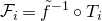 $\mathcal {F}_i = \tilde {f}^{-1}\circ T_i$
. The following can be checked by straightforward induction on
 $n$
.
Proposition A.1.
Let
 $\tilde {x} \in {\mathbb {R}^2}$
,
 $v \in {\mathbb {Z}^2}$
, and
 $\boldsymbol {\omega }, \boldsymbol {\tau } \in \Sigma$
. Then the following are equivalent:
-
(1)
$\psi _v(\boldsymbol {\omega }) = \boldsymbol {\tau }$
; -
(2)
$\mathcal {F}_{\tau _n} \circ \cdots \circ \mathcal {F}_{\tau _1} (\tilde {x}+v) -\mathcal {F}_{\omega _n} \circ \cdots \circ \mathcal {F}_{\omega _1}(\tilde {x}) \in {\mathbb {Z}^2}$
for every
$n\geq 1$
; -
(3)
$\mathcal {F}_{\tau _n} \circ \cdots \circ \mathcal {F}_{\tau _1} (\tilde {x}+v) -\mathcal {F}_{\omega _n} \circ \cdots \circ \mathcal {F}_{\omega _1}(\tilde {x}) = u_n$
for every
$n\geq 1$
.





In other words, calculating pre-orbits of a point
 $x \in \mathbb {T}^2$
can be done using a representative
 $\tilde {x} \in {\mathbb {R}^2}$
and an appropriate sequence of maps
 $\mathcal {F}_1, \dots , \mathcal {F}_d$
. However, the sequence of maps to be used depends on the representative
 $\tilde {x}$
, and the map
 $\psi _v$
describes how the sequence changes when using the representative
 $\tilde {x}+v$
instead of
 $\tilde {x}$
.
A.3 A canonical homeomorphism
$\operatorname {Sol} \to {\mathbf {L}_{f}}$

We define a map
 $\tilde {\phi }: {\mathbb {R}^2} \times \Sigma \to {\mathbf {L}_{f}}$
by setting
 \begin{equation*}\tilde {\phi } (\tilde {x}, \omega _1, \omega _2, \ldots ) = (x_0, x_1, x_2, \ldots ),\end{equation*}
where
 \begin{equation} x_i = \pi _{cov} \circ \mathcal {F}_{\omega _i} \circ \cdots \circ \mathcal {F}_{\omega _1} (\tilde {x}). \end{equation}
It follows from (29) that
 $\tilde {\phi }$
is
 $G$
-invariant, i.e.
 \begin{equation*}\tilde {\phi }(\tilde {x}, \boldsymbol {\omega }) = \tilde {\phi }(\tilde {x}+v, \psi _{v}(\boldsymbol {\omega }))\end{equation*}
for every
 $v \in {\mathbb {Z}^2}$
. Hence
 $\tilde {\phi }$
induces a map
 $\phi : \operatorname {Sol} \to {\mathbf {L}_{f}}$
such that
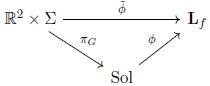
commutes.
Proposition A.2.
The map
 $\phi$
is a homeomorphism.
Proof.
Proposition A.1 implies that
 $\tilde {\phi }(\tilde {x}, \boldsymbol {\omega }) = \tilde {\phi }(\tilde {y}, \boldsymbol {\tau })$
if and only if
 $(\tilde {x}, \boldsymbol {\omega })$
and
 $(\tilde {y}, \boldsymbol {\tau })$
lie in the same
 $G$
-orbit. Moreover, it is clear that
 $\tilde {\phi }$
is a continuous surjection. Hence (see [Reference RotmanRot88, Corollary 1.10 and Example 1.5]) it suffices to show that
 $\tilde {\phi }$
is an open mapping. To see why
 $\tilde {\phi }$
is open it suffices to check that the image under
 $\tilde {\phi }$
of open rectangles of the form
 \begin{equation} U \times C(\omega _1, \ldots , \omega _n) \end{equation}
are open, as these form a basis of the topology on
 ${\mathbb {R}^2} \times \Sigma$
. Now, the image of (31) under
 $\tilde {\phi }$
is
 \begin{equation} {\mathbf {L}_{f}} \cap \{ (x_1, x_2, \ldots ) \in (\mathbb {T}^2)^{\mathbb {N}}: x_i \in U_i \text { for }1\leq i \leq n\}, \end{equation}
where
 \begin{equation} U_i = \pi _{\mathrm {cov}} \circ \mathcal {F}_{\omega _n} \circ \cdots \circ \mathcal {F}_{\omega _1}(U). \end{equation}
Since the right-hand side of (33) is a composition of open mappings, it follows that (32) is open in
 $\mathbf {L}_{f}$
.
In view of Proposition A.2, the natural extension
 ${\hat {f}} : {\mathbf {L}_{f}} \to {\mathbf {L}_{f}}$
induces a homeomorphism
 $Sf: \operatorname {Sol} \to \operatorname {Sol}$
by setting
 $Sf = \phi ^{-1} \circ {\hat {f}} \circ \phi$
. It turns out that
 $Sf$
itself has a very natural expression, which we now describe.
Let
 $F, F^{\sharp }: {\mathbb {R}^2} \times \Sigma \to {\mathbb {R}^2} \times \Sigma$
be the maps
 \begin{align*} (\tilde {x}, \omega _1, \omega _2, \ldots ) & \overset {F}{\mapsto } (\tilde {f}(\tilde {x}), 1, \omega _1, \omega _2, \ldots ), \\ (\tilde {x}, \omega _1, \omega _2, \ldots ) & \overset {F^\sharp }{\mapsto } (\mathcal {F}_{\omega _1}(\tilde {x}), \omega _2, \omega _3, \dots ). \end{align*}
(Recall that we have chosen the
 $w_i$
so that
 $[w_1]= [\underline {0}]$
.) The map
 $F$
is not surjective and the map
 $F^\sharp$
is not injective, but
 $F^\sharp \circ F$
is the identity on
 ${\mathbb {R}^2} \times \Sigma$
. The following proposition follows straight from the definitions of
 $\phi$
and
 $Sf$
.
Proposition A.3.
The map
 $Sf$
is given by
 \begin{equation*}Sf([(\tilde {x}, \boldsymbol {\omega })]_G) = [F(\tilde {x}, \boldsymbol {\omega })]_G.\end{equation*}
The inverse of
 $Sf$
is given by
 \begin{equation*}Sf^{-1}([(\tilde {x}, \boldsymbol {\omega })]_G) = [F^\sharp (\tilde {x}, \boldsymbol {\omega })]_G.\end{equation*}
The construction of
 $\operatorname {Sol}$
and its dynamics
 $Sf$
is clarified by the following commuting diagram.
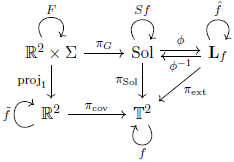
A.4 Invariant measures on
$\operatorname {Sol}$

Generally speaking, if
 $(\tilde {X}, p)$
is a covering spaceFootnote
6
of
 $X$
, then any (Borel) measure
 $\mu$
on
 $X$
induces a unique (Borel) measure
 $\tilde {\mu }$
on
 $ \tilde {X}$
by setting
 $\tilde {\mu }(A) = \mu (p(A))$
whenever
 $p \vert A$
is injective, and extending it accordingly. We refer to
 $\mu$
as the lift of
 $\mu$
. Such a measure is necessarily invariant under any deck transformation of the covering.
Conversely, any measure
 $\tilde {\mu }$
on
 $\tilde {X}$
invariant under deck transformations is the lift of a unique measure
 $\mu$
on
 $X$
. We say that
 $\tilde {\mu }$
descends to
 $\mu$
whenever this is the case. Note that
 $\tilde {\mu }$
descends to
 $\mu$
if and only if
 $\mu = p_*(\tilde {\mu } \vert D)$
where
 $D$
is a fundamental domain of the covering space.
Now suppose we have a second covering space
 $(\tilde {Y}, q)$
of some space
 $Y$
and maps
 $\tilde {\pi }: \tilde {Y} \to \tilde {X}$
,
 $\pi : Y \to X$
such that
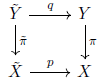
commutes. If
 $\nu$
is a measure on
 $Y$
which lifts to
 $\tilde {\nu }$
on
 $\tilde {Y}$
, then
 $\tilde {\pi }_* \tilde {\nu } = \tilde {\mu }$
if and only if
 $\pi _*\nu = \mu$
.
It is well known that, given any
 $f$
-invariant measure, there is precisely one
 $\hat {f}$
-invariant measure which projects on
 $\mathbb {T}^2$
by
 $\pi _{\mathrm {ext}}$
. Now, since
 $Sf$
is conjugated to
 $\hat {f}$
and
 $\pi _{\mathrm {ext}} \circ \phi = \pi _{\operatorname {Sol}}$
, it follows that there is precisely one
 $Sf$
-invariant measure
 $\boldsymbol {\mu }$
on
 $\operatorname {Sol}$
which projects to
 $\mu$
through
 $\pi _{\operatorname {Sol}}$
. One of the advantages of working with
 $\operatorname {Sol}$
rather than with
 $\mathbf {L}_{f}$
is that
 $\boldsymbol {\mu }$
has a particularly intuitive description.
Let
 $\tilde {{\boldsymbol {\mu }}}$
be the lift of
 $\boldsymbol {\mu }$
to
 ${\mathbb {R}^2} \times \Sigma$
and
 $\tilde {\mu }$
the lift of
 $\mu$
on
 $\mathbb {R}^2$
. Since
 $(\pi _{\operatorname {Sol}})_*{\boldsymbol {\mu }} = \mu$
we must have that
 $(\operatorname {proj}_1)_* \tilde {{\boldsymbol {\mu }}} = \tilde {\mu }$
. In other words,
 \begin{equation*}\tilde {{\boldsymbol {\mu }}}(A \times \Sigma ) = \tilde {\mu }(A)\end{equation*}
for every measurable
 $A \subset {\mathbb {R}^2}$
. Invariance of
 $\boldsymbol {\mu }$
under
 $Sf$
, together with Proposition A.3, implies that
 \begin{equation} \tilde {{\boldsymbol {\mu }}}(A \times C(\omega _1, \ldots , \omega _n)) = \tilde {\mu }(\mathcal {F}_{\omega _n} \circ \cdots \circ \mathcal {F}_{\omega _1}(A)). \end{equation}
Here
 $C(\omega _1, \ldots , \omega _n)$
denotes the cylinder set
 \begin{equation*}\{(\tau _1, \tau _2, \ldots ) \in \Sigma : \tau _i = \omega _i \text { for } 1 \leq i \leq n \}.\end{equation*}
Sets of the form
 $A \times C(\omega _1, \ldots , \omega _n)$
form a semi-ring which generates the Borel
 $\sigma$
-algebra on
 ${\mathbb {R}^2} \times \Sigma$
. Hence (35) determines
 $\tilde {{\boldsymbol {\mu }}}$
.
Remark A.2. If we did not already know about the existence of
 $\boldsymbol {\mu }$
, we could simply lift
 $\mu$
to
 $\tilde {\mu }$
and use (35) to define
 $\tilde {{\boldsymbol {\mu }}}$
on
 ${\mathbb {R}^2} \times \Sigma$
. This measure, by construction, is
 $G$
-invariant and descends to an
 $Sf$
-invariant measure
 $\boldsymbol {\mu }$
on
 $\operatorname {Sol}$
, which in turn projects to
 $\mu$
through
 $\pi _{\operatorname {Sol}}$
. Again, since any such measure must satisfy (35), it is the unique
 $Sf$
-invariant measure with this property.
Below is a schematic illustration of how
 $\mu$
,
 $\hat {\mu }$
,
 $\tilde {\mu }$
,
 $\boldsymbol {\mu }$
, and
 $\tilde {{\boldsymbol {\mu }}}$
are related. A filled arrow (
 $\rightarrow$
) indicates that measures are related by push-forward, whereas a dashed arrow (
 $\dashrightarrow$
) indicates that the former descends to the latter.
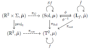
Remark A.3. The maps
 $\tilde {f}: {\mathbb {R}^2} \to {\mathbb {R}^2}$
and
 $F: {\mathbb {R}^2} \times \Sigma \to {\mathbb {R}^2} \to \Sigma$
have been left out from (36) as they are not measure-preserving. Indeed
 $\tilde {f}$
is invertible on
 $\mathbb {R}^2$
and has a Jacobian strictly larger than
 $1$
with respect to
 $\tilde {\mu }$
. The push-forward of
 $\tilde {{\boldsymbol {\mu }}}$
under
 $F$
is the restriction of
 $\tilde {{\boldsymbol {\mu }}}$
to
 ${\mathbb {R}^2} \times C(\omega _1)$
(the image of
 $F$
).
A.5 Lifting the Haar measure to
$\operatorname {Sol}$

We now turn to the particular case in which
 $\mu$
is the Haar measure on
 $\mathbb {T}^2$
. Its lift
 $\tilde {\mu }$
on
 $\mathbb {R}^2$
is the Lebesgue measure. Hence (35) can be written as
 \begin{align} \tilde {{\boldsymbol {\mu }}}(A\times C(\omega _1, \dots , \omega _n)) & = \int _{A} |\!\det D (\mathcal {F}_{\omega _n} \circ \cdots \circ \mathcal {F}_{\omega _1})(\tilde {x})| \ d\tilde {\mu }(\tilde {x}) \end{align}
 \begin{align} & = \int _A \tilde {{\boldsymbol {\mu }}}_{\tilde {x}} (C(\omega _1, \ldots \omega _n))\, d\tilde {\mu }(\tilde {x}), \end{align}
where
 $\tilde {{\boldsymbol {\mu }}}_{\tilde {x}}$
is the unique measure on
 $\Sigma$
such that
 \begin{equation} \tilde {{\boldsymbol {\mu }}}_{\tilde {x}} (C(\omega _1, \ldots \omega _n)) = |\!\det D (\mathcal {F}_{\omega _n} \circ \cdots \circ \mathcal {F}_{\omega _1})(\tilde {x}) | \end{equation}
for each cylinder
 $C(\omega _1, \ldots , \omega _n)$
.
The right-hand side of (39) is a
 $G$
-invariant function on
 ${\mathbb {R}^2} \times \Sigma$
. Hence
 \begin{equation*}(\psi _v)_* \tilde {{\boldsymbol {\mu }}}_{\tilde {x}} = \tilde {{\boldsymbol {\mu }}}_{\tilde {x} + v}\end{equation*}
for every
 $v \in {\mathbb {Z}^2}$
, and
 $\tilde {{\boldsymbol {\mu }}}_{\tilde {x}}$
descends to a measure
 ${\boldsymbol {\mu }}_{x}$
on
 $\operatorname {Sol}$
, where
 $x = \pi _{\mathrm {cov}}(\tilde {x})$
. The push-forward
 ${\hat {\mu }}_x$
of this measure under
 $\phi$
is the same as the push-forward of
 $\tilde {{\boldsymbol {\mu }}}_{\tilde {x}}$
under
 $\tilde {\phi }$
. Of course, for every
 $(\tilde {x}, \omega _1, \omega _2, \ldots ) \in \tilde {\phi }^{-1}(x_0, x_1, \ldots )$
and every
 $n \geq 1$
we have
 \begin{equation*}|\!\det D (\mathcal {F}_{\omega _n} \circ \cdots \circ \mathcal {F}_{\omega _1})(\tilde {x})| = |\!\det D f^n(x_n)|^{-1},\end{equation*}
so that
 \begin{equation} {\hat {\mu }}_x(\{ (\xi _1, \xi _2, \ldots ) \in {\mathbf {L}_{f}} : \xi _n = x_n \}) = |\!\det Df^n(x_n)|^{-1}. \end{equation}
Extending (37) to the full
 $\sigma$
-algebra on
 ${\mathbb {R}^2} \times \Sigma$
and descending to
 $\operatorname {Sol}$
gives
 \begin{equation} {\boldsymbol {\mu }}(A) = \int _{\mathbb {T}^2} {\boldsymbol {\mu }}_x(A) \, d\mu (x) \end{equation}
for every measurable
 $A \subset \operatorname {Sol}$
. Similarly,
 \begin{equation} \mu (A) = \int _{\mathbb {T}^2} {\hat {\mu }}_x(A) \, d\mu (x) \end{equation}
for every measurable
 $A \subset {\mathbf {L}_{f}}$
.
A.6 Continuity
The measures
 $\hat {\mu }$
,
 ${\hat {\mu }}_x$
,
 ${\boldsymbol {\mu }}_x$
,
 $\tilde {{\boldsymbol {\mu }}}_{\tilde {x}}$
,
 $\boldsymbol {\mu }$
and
 $\tilde {{\boldsymbol {\mu }}}$
all depend on the map
 $f$
. Let us stress this dependence by calling them
 ${\hat {\mu }}^f$
,
 ${\hat {\mu }}_x^f$
,
 ${\boldsymbol {\mu }}_x^f$
,
 $\tilde {{\boldsymbol {\mu }}}_{\tilde {x}}^f$
 ${\boldsymbol {\mu }}^f$
and
 $\tilde {{\boldsymbol {\mu }}}^f$
instead. The following is obvious from (37), (39), (40) and (41).
Proposition A.4.
The measures
 ${\hat {\mu }}_x^f$
,
 ${\boldsymbol {\mu }}_x^f$
,
 $\tilde {{\boldsymbol {\mu }}}_{\tilde {x}}^f$
 ${\boldsymbol {\mu }}^f$
and
 $\tilde {{\boldsymbol {\mu }}}^f$
depend continuously on
 $f$
in the weak* topology in their respective spaces, when seen as maps from
 $\operatorname {End}_\mu ^1(\mathbb {T}^2)$
. Moreover, the measures
 ${\hat {\mu }}_x^f$
,
 ${\boldsymbol {\mu }}_x^f$
and
 $\tilde {{\boldsymbol {\mu }}}_{\tilde {x}}$
vary continuously with
 $x$
in the weak* topology in their respective spaces, when seen as maps from
 $\mathbb {T}^2$
and
 $\mathbb {R}^2$
, respectively.
If we consider the measure
 ${\hat {\mu }}^f$
as a measure on
 $(\mathbb {T}^2)^{\mathbb {Z}_+}$
, supported on
 $\mathbf {L}_{f}$
, rather than a measure on
 $\mathbf {L}_{f}$
itself, then this measure also varies continuously with
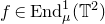 $f \in \operatorname {End}_\mu ^1(\mathbb {T}^2)$
.
A.7 Projective bundles
Each of the spaces
 $\mathbf {L}_{f}$
,
 $\operatorname {Sol}$
and
 ${\mathbb {R}^2} \times \Sigma$
comes with a trivial bundle
 \begin{align*} & {\mathbb {P}} {\mathbf {L}_{f}} = {\mathbf {L}_{f}} \times {\mathbb {P}} {\mathbb {R}^2}, \\ & {\mathbb {P}} \operatorname {Sol} = \operatorname {Sol} \times {\mathbb {P}} {\mathbb {R}^2}, \\ & {\mathbb {P}} ({\mathbb {R}^2} \times \Sigma ) = {\mathbb {R}^2} \times \Sigma \times {\mathbb {P}} {\mathbb {R}^2}. \end{align*}
On each of these bundles, the derivative of
 $f$
induces bundle maps
 $P{\hat {f}}$
,
 $PSf$
and
 $PF$
given, respectively, by
 \begin{align*} (\hat {x}, [v]) & \overset {{\scriptstyle{P{\hat {f}}}}}{\mapsto } ({\hat {f}}(\hat {x}), [Df_{\pi _{\mathrm {ext}}(\hat {x})} v]), \\ ([\tilde {x}, \boldsymbol {\omega }]_G, [v]) & \overset {PSf}{\mapsto } (Sf ([\tilde {x}, \boldsymbol {\omega }]_G), [Df_{\tilde {x}} v]), \\ (\tilde {x}, \boldsymbol {\omega }, [v]) & \overset {PF}{\mapsto } (F(\tilde {x}, \boldsymbol {\omega }), [Df_{\tilde {x}} v]) \end{align*}
Let
 $i$
be the identity map on
 ${\mathbb {P}} {\mathbb {R}^2}$
. Then the following diagram commutes.
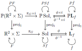
A
 $PS f$
-invariant measure
 ${\boldsymbol {\mu }}^p$
corresponds to a
 $P {\hat {f}}$
-invariant measure
 ${\hat {\mu }}^p = (\phi , i)_*{\boldsymbol {\mu }}^p$
and vice versa. Moreover,
 ${\boldsymbol {\mu }}^p$
lifts to a unique measure
 $\tilde {{\boldsymbol {\mu }}}^p$
on
 ${\mathbb {P}}({\mathbb {R}^2} \times \Sigma )$
through
 $\pi _G \times i$
, which is the same as the lift of
 ${\hat {\mu }}^p$
through
 $\tilde {\phi }\times i$
. This measure is not invariant under
 $PF$
(see Remark A.3). However, we have the following proposition.
Proposition A.5.
Given a measure
 ${\boldsymbol {\mu }}^{p}$
on
 ${\mathbb {P}} \operatorname {Sol}$
and a sequence of measures
 ${\boldsymbol {\mu }}_n^{p}$
on
 ${\mathbb {P}} \operatorname {Sol}$
with corresponding lifts
 $\tilde {{\boldsymbol {\mu }}}^{p}$
and
 $\tilde {{\boldsymbol {\mu }}}_n^{p}$
on
 ${\mathbb {P}} ({\mathbb {R}^2} \times \Sigma )$
, we have that
 ${\boldsymbol {\mu }}_n^{p}$
converges (weakly*) to
 ${\boldsymbol {\mu }}^{p}$
if and only if
 $\tilde {{\boldsymbol {\mu }}}_n^{p}$
converges (weakly*) to
 $\tilde {{\boldsymbol {\mu }}}^{p}$
.
Now,
 $\tilde {{\boldsymbol {\mu }}}_n^p$
and
 $\tilde {{\boldsymbol {\mu }}}^p$
are all
 $G \times \{i\}$
-invariant. Therefore, to say that
 $\tilde {{\boldsymbol {\mu }}}_n^p$
converges to
 $\tilde {{\boldsymbol {\mu }}}^p$
it suffices to show that
 $\tilde {{\boldsymbol {\mu }}}_n^p \vert Q$
converges to
 $\tilde {{\boldsymbol {\mu }}}^p \vert Q$
, where
 $Q \subset {\mathbb {P}} ({\mathbb {R}^2} \times \Sigma )$
is any set containing a fundamental domain of the action
 $G \times \{ i \}$
and satisfying
 $\tilde {{\boldsymbol {\mu }}}^p( \partial Q)=0.$
In the proof of Theorem C we do this by taking
 $Q = [0,1] \times \Sigma \times {\mathbb {P}} {\mathbb {R}^2}$
.
Acknowledgment
We thank the anonymous referee for the useful comments and suggestions.
Conflicts of interest
None.
Financial support
MA was partially supported by AMSUD220029, PDC was partially supported by CNPq 403041/2021-0 and AMSUD220029, and RS was partially supported by Fondecyt 1230632 and AMSUD220029.
Journal information
Compositio Mathematica is owned by the Foundation Compositio Mathematica and published by the London Mathematical Society in partnership with Cambridge University Press. All surplus income from the publication of Compositio Mathematica is returned to mathematics and higher education through the charitable activities of the Foundation, the London Mathematical Society and Cambridge University Press.