





Impact Statement
Reinforced concrete shear walls are widely used in seismic regions to provide lateral stiffness and control structural deformations during earthquakes. Accurate estimation of drift capacity is critical for seismic assessment and design because it is directly related to damage levels, safety evaluation, and collapse prevention. Traditional empirical formulas are often based on limited datasets and simplified assumptions, which may reduce their accuracy for walls with different geometries and reinforcement configurations. This study develops tree-based machine learning models for predicting drift capacity using an experimental database of 208 reinforced concrete shear walls. The models capture nonlinear relationships governing deformation capacity and show strong predictive performance, supporting data-driven approaches as complementary tools for seismic assessment and performance-based design.
1. Introduction
Reinforced concrete (RC) shear walls are widely used as primary lateral force-resisting elements in seismic regions. In earthquake-prone countries, wall-type structural systems are frequently adopted because of their high stiffness and their ability to control lateral displacements. By limiting inter-story drifts, shear walls contribute significantly to preventing excessive structural damage or collapse.
In Romania, structural walls became common especially in the post-war period. Many residential buildings constructed between the 1960s and 1977 relied on wall-type systems, including both cast-in-place and prefabricated solutions (Balan et al., Reference Balan, Cristescu and Cornea1982). The 4 March 1977 Vrancea earthquake provided a country-wide verification of their performance. Due to the lack of available data, the design provisions at that time were based on response spectra that, following the earthquake, were found to be inconsistent with the specific characteristics of Vrancea subcrustal ground motions, particularly in Bucharest and the surrounding areas of south-eastern Romania. Although some buildings with reinforced concrete structural walls exhibited satisfactory overall performance, others sustained severe damage, and a newly constructed multistory shear wall building in Bucharest even collapsed. The design and construction practices at that time, constrained by the contemporary state of knowledge, also contributed to these effects (Berg et al., Reference Berg, Bolt, Sozen and Rojahn1980).
Currently, RC shear walls continue to be widely used as a lateral force-resisting system not only in the design of new structures, but also in seismic retrofitting. In Romania, the addition of new RC shear walls is one of the most frequently used strengthening measures for existing buildings, mainly to increase stiffness and reduce inter-story drift demands. Given that a significant portion of the building stock consists of wall-type systems, understanding their deformation capacity is essential. Drift capacity is a key parameter in both assessment and design; however, predicting it is not straightforward. The response of RC shear walls depends on geometry, axial load, reinforcement detailing, material properties, and failure mode. Flexure-dominated, shear-dominated, and mixed mechanisms may develop, sometimes leading to abrupt degradation. Experimental evidence shows that similar drift ratios may correspond to very different damage states (Yahyapour et al., Reference Yahyapour, Azhari and Hamidia2026), which highlights the limits of simplified deformation-based criteria. Netrattana et al. (Reference Netrattana, Taleb, Watanabe, Kono, Mukai, Tani and Sakashita2017) showed, through a parametric fiber-based investigation, that the ultimate drift capacity of RC shear walls is particularly sensitive to axial load ratio, while concrete strength, transverse reinforcement, and boundary region dimensions also affect the response. Their results further emphasized that increasing axial load can significantly reduce drift capacity, whereas improved confinement and larger boundary regions may enhance it.
Over the past decades, several empirical and analytical expressions have been proposed to estimate deformation capacity. While they are practical, they are often derived from limited datasets and rely on simplified assumptions. When applied to walls with different geometries or reinforcement layouts, their accuracy may decrease. In the present study, the predictive capability of the well-known empirical formulation proposed by Abdullah and Wallace (Reference Abdullah and Wallace2019) is also examined and compared with data-driven approaches. Related studies have also pointed out that deformation capacity differs markedly between wall classes. Pavel et al. (Reference Pavel, Panfilii and Farsangi2020) evaluated the displacement capacity of RC shear walls using both experimental and analytical data. Their study showed that squat walls have mean and median ultimate drift ratios approximately half of those of slender walls. Segura and Wallace (Reference Segura and Wallace2018) further showed that, for slender walls, drift capacity is strongly influenced not only by confinement detailing but also by wall thickness, wall length, and compression depth, with thin walls being particularly prone to limited deformation capacity.
Machine learning (ML) techniques have recently been used to model complex structural behavior directly from data. Yahyapour et al. (Reference Yahyapour, Azhari and Hamidia2026) proposed a multi-criteria seismic damage evaluation framework for RC columns using a combination of unsupervised clustering and supervised learning. Their study showed that damage states cannot be reliably defined using drift ratio alone, since stiffness and strength degradation may vary significantly at the same drift level. Although focused on RC columns, the conclusions of the cited work are also relevant to shear walls, as they exhibit quite similar nonlinear degradation under cyclic loading.
For RC shear walls, Solórzano and Plevris (Reference Solorzano and Plevris2022) developed artificial neural network surrogate models to estimate lateral load capacity, with accuracy comparable to nonlinear finite element analyses while significantly reducing computational cost. Aladsani et al. (Reference Aladsani, Burton, Abdullah and Wallace2022) applied Extreme Gradient Boosting (XGBoost) to predict the drift capacity of RC shear walls and combined it with SHAP analysis to interpret model predictions. Luo and Paal (Reference Luo and Paal2019) proposed a locally weighted support vector machine model for predicting the plastic rotational capacity of RC columns, while Nguyen et al. (Reference Nguyen, Thai and Kim2020) used artificial neural networks to develop an empirical equation for predicting the axial capacity of circular CFST columns, demonstrating improved accuracy compared to traditional equations proposed by the current design codes. Yu et al. (Reference Yu, Chen, Liao, Wang, Zhang, Kang and Lu2025) introduced a data-driven framework for RC shear wall design by training generative adversarial network (GAN) models based on building plan geometry and seismic code criteria, and combined it with SHAP analysis to identify the most influential parameters. Machine learning has also been applied more broadly in earthquake engineering. Damikoukas and Lagaros (Reference Damikoukas and Lagaros2025) improved seismic response prediction of building systems using deep learning. Logistic regression has been used for seismic fragility assessment of bridges (Kameshwar and Padgett, Reference Kameshwar and Padgett2017), soil-structure systems (Koutsourelakis, Reference Koutsourelakis2010), and reinforced concrete shear walls (Yazdi et al., Reference Yazdi, Haukaas, Yang and Gardoni2016). Reviews by Xie et al. (Reference Xie, Sichani, Padgett and DesRoches2020) underline the increasing role of ML in modeling complex seismic behavior. Barkhordari et al. (Reference Barkhordari, Qi and Khoshnazar2025) showed that hybrid machine learning models can predict the shear strength of flanged squat RC shear walls more accurately than conventional code-based equations. Their results also highlighted the important role of wall geometry, concrete strength, reinforcement ratios, and axial load in controlling the predicted response.
However, limitations still persist. Existing datasets for RC shear walls are often limited or heterogeneous, while the reliability of machine learning predictions also depends strongly on the adopted model-development and validation strategy. In particular, a clear separation between hyperparameter optimization and final model assessment is required to obtain a reliable estimate of predictive performance on unseen data. More robust validation strategies are therefore needed to reduce model-selection bias and improve confidence in model generalization. In a previous study conducted by the authors (Kadhim and Craifaleanu, Reference Kadhim and Craifaleanu2025), machine learning models were applied to both RC columns and shear walls. The results showed that prediction performance depends strongly on dataset consistency and cross-sectional topology.
Beyond their use as standalone prediction tools, data-driven models may also support performance-based assessment and structural optimization procedures in which multiple structural configurations need to be evaluated efficiently. Recent research on performance-based optimization of frame-wall systems has highlighted the role of shear-wall characteristics in controlling structural response and has considered wall configuration within the optimization process (Olivo et al., Reference Olivo, Cucuzza, Domaneschi, Gao and Marano2025). In this context, rapid estimates of wall deformation capacity could provide an additional screening tool for comparing candidate structural configurations before more computationally demanding analyses are performed.
Based on these observations, the present study focuses exclusively on RC shear walls with rectangular and I-shaped cross-sections, for which a sufficiently large and consistent experimental database is available. A dataset of 208 cyclically tested RC shear walls was derived from the ACI 445B Shear Wall Database (Pujol et al., Reference Pujol, Song, Wang, Puranam and Usta2019). The target variable is the drift capacity, derived from the displacement corresponding to 80% of the maximum lateral strength on the descending portion of the load–displacement envelope and normalized by the corresponding lateral loading height. The objective of this paper is to develop and evaluate tree-based machine learning models for predicting the drift capacity of RC shear walls. Three individual learners, that is, Extra Trees (Extremely Randomized Trees), Random Forest, and XGBoost (Extreme Gradient Boosting), are optimized using nested cross-validation within the model development subset. To further enhance predictive accuracy and stability, a stacking ensemble is constructed by combining the outputs of the individual models.
The complete dataset is divided once into an 80% development subset and a 20% independent hold-out test subset, with the split stratified using quantile-based groups of the target variable to maintain an adequate representation of the drift-capacity range. Model development and hyperparameter optimization are performed exclusively within the development subset using a nested fivefold cross-validation framework, while the hold-out subset remains unseen until the final evaluation. Model performance is assessed using R 2, MAE, and RMSE. In addition, the predictive performance of the machine learning models is compared with the empirical formulation proposed by Abdullah and Wallace. This comparison provides a practical reference point for evaluating the relative behavior of traditional empirical expressions and data-driven approaches when applied to reinforced concrete shear walls.
2. Database
2.1. Shear wall experimental database
The present study focuses exclusively on RC shear walls with rectangular and I-shaped cross-sections. Studies were performed using data derived from the ACI 445B Shear Wall Database (Pujol et al., Reference Pujol, Song, Wang, Puranam and Usta2019).
From this database, a processed subset of 231 RC shear wall specimens containing the parameters required for the present analysis was considered, including walls with rectangular, I-shaped, T-shaped, and general cross-sectional configurations. Only walls with rectangular and I-shaped sections were retained. Walls with T-shaped or general cross-sections were excluded due to their limited representation in the available experimental data, which could introduce bias and increase uncertainty in the training of machine learning models. This filtering resulted in a final database of 208 RC shear wall specimens, consisting of 106 rectangular walls and 102 I-shaped walls. The complete processed database, including the identifiers linking each specimen to the corresponding records in the ACI 445B Shear Wall Database and the assignment of each specimen to the development and hold-out test subsets, is provided as Supplementary Material and is also openly available on Zenodo (Kadhim and Craifaleanu, Reference Kadhim and Craifaleanu2026).
All selected specimens were subjected to quasi-static cyclic lateral loading, typically applied at the top of the wall while maintaining a constant axial load. Boundary conditions were generally idealized as fixed at the base, consistent with standard experimental configurations for cantilever-type shear wall testing. Only specimens with complete geometric, mechanical, and reinforcement data were included in the final database to ensure uniformity during model training and evaluation.
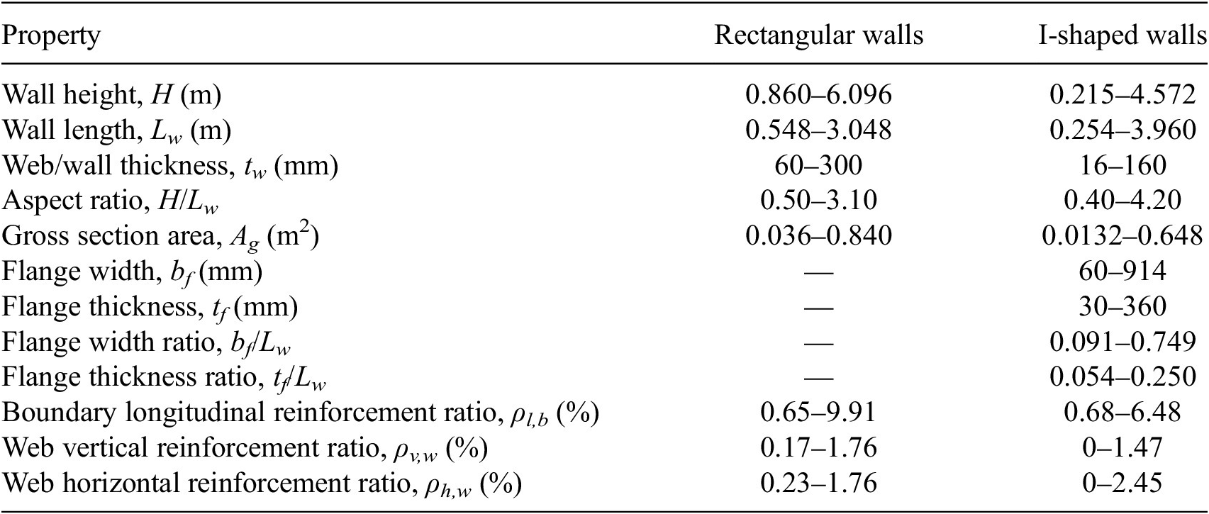
To provide a more direct physical characterization of the final dataset, Table 1 summarizes the ranges of the main geometric dimensions and reinforcement ratios separately for rectangular and I-shaped walls. For I-shaped specimens, flange dimensions and their proportions relative to the total wall length are also reported.
Geometric and reinforcement characteristics of the final RC shear wall database

Table 1. Long description
The table lists 12 properties with minimum-maximum ranges for two categories: Rectangular walls and I-shaped walls.
* Wall height, H (m): Rectangular 0.860 to 6.096; I-shaped 0.215 to 4.572.
* Wall length, L sub w (m): Rectangular 0.548 to 3.048; I-shaped 0.254 to 3.960.
* Web or wall thickness, t sub w (mm): Rectangular 60 to 300; I-shaped 16 to 160.
* Aspect ratio, H over L sub w: Rectangular 0.50 to 3.10; I-shaped 0.40 to 4.20.
* Gross section area, A sub g (m super 2): Rectangular 0.036 to 0.840; I-shaped 0.0132 to 0.648.
* Flange width, b sub f (mm): Rectangular is not applicable; I-shaped 60 to 914.
* Flange thickness, t sub f (mm): Rectangular is not applicable; I-shaped 30 to 360.
* Flange width ratio, b sub f over L sub w: Rectangular is not applicable; I-shaped 0.091 to 0.749.
* Flange thickness ratio, t sub f over L sub w: Rectangular is not applicable; I-shaped 0.054 to 0.250.
* Boundary longitudinal reinforcement ratio, rho sub l,b (percent): Rectangular 0.65 to 9.91; I-shaped 0.68 to 6.48.
* Web vertical reinforcement ratio, rho sub v,w (percent): Rectangular 0.17 to 1.76; I-shaped 0 to 1.47.
* Web horizontal reinforcement ratio, rho sub h,w (percent): Rectangular 0.23 to 1.76; I-shaped 0 to 2.45.
Note. Values are reported as minimum-maximum ranges. bf and tf denote flange width and flange thickness, respectively.
2.2. Input parameters and output variable
The input parameters used in this study were selected based on their documented influence on the seismic response and deformation capacity of RC shear walls, as observed in prior experimental and analytical research. The following variables were adopted as predictors:
-
• ratio between wall length and thickness (Lw/tw);
-
• normalized shear coefficient (V/Agfc);
-
• axial load ratio (P/Agfc);
-
• maximum ratio of transverse reinforcement spacing to vertical bar diameter (s/db);
-
• ratio of ultimate to yield strength of boundary longitudinal reinforcement (fu/fy);
-
• longitudinal reinforcement ratio in boundary regions and web (ρ l);
-
• transverse reinforcement ratio (ρw);
-
• cross-sectional shape (rectangular or I-shaped).
These parameters collectively describe the geometric slenderness, loading conditions, reinforcement detailing, and material strength characteristics governing the nonlinear response of RC shear walls under cyclic loading.
Failure mode was not included as an input variable in the present model. Although the deformation capacity of RC shear walls is strongly influenced by whether the response is predominantly flexural, shear-controlled, or governed by a mixed mechanism, a consistent three-class failure-mode classification was not available for the complete dataset. The source database provides a binary “Shear Damage” field indicating whether the original researcher attributed the cause of failure to shear, but this information is unavailable for a substantial portion of the retained specimens and does not distinguish consistently between flexural and mixed flexure-shear mechanisms.
The output variable considered in this study is the drift capacity, defined as the lateral displacement at the intersection of the horizontal line corresponding to 80% of the maximum lateral strength, 0.8Vmax, with the descending branch of the load–displacement envelope, as defined in the ACI 445B Shear Wall Database (Pujol et al., Reference Pujol, Song, Wang, Puranam and Usta2019). The displacement capacity reported in the source database was normalized by the corresponding lateral loading height and expressed as a percentage.
2.3. Statistical ranges and exploratory data analysis
The statistical characteristics and variability of the input parameters were investigated using histograms and scatter plots illustrating their relationship with the drift capacity, as summarized in Figures 1 and 2.
Statistical distributions of the input parameters for RC shear walls, shown as histograms.

Figure 1. Long description
The figure consists of eight panels labeled a through h. Each panel plots Frequency on the y-axis against a specific structural parameter on the x-axis.
* Panel a: L w forward slash t w. A bimodal distribution with peaks near 12 and 22, ranging from 5 to 45.
* Panel b: Shear coefficient. A right-skewed distribution peaking between 0.05 and 0.10, extending to 0.25.
* Panel c: Axial ratio. A highly skewed distribution with a dominant peak near 0.00, tapering off significantly by 0.15.
* Panel d: Maximum s forward slash d b. An irregular distribution with peaks at 0.0, 5.0, 8.0, and a final spike at 20.0.
* Panel e: f u forward slash f y vertical reinforcement. A distribution with a primary peak at 1.4 and smaller clusters between 1.1 and 1.7.
* Panel f: Boundary vertical reinforcement ratio. A right-skewed distribution with a major peak at 0.015 and a secondary peak at 0.025, trailing off toward 0.10.
* Panel g: Web vertical reinforcement ratio. A right-skewed distribution peaking at 0.0025, with most data points below 0.0100.
* Panel h: Web horizontal reinforcement ratio. A right-skewed distribution peaking between 0.002 and 0.006, with a long tail extending to 0.025.
Relationships between the input parameters and drift capacity for RC shear walls, shown as scatter plots.

Figure 2. Long description
The figure consists of eight panels arranged in a two-column by four-row grid. All panels share a common x-axis labeled Drift capacity percentage, ranging from 0 to 9.
* Panel a: Y-axis is L w forward slash t w, ranging from 5 to 45. Data points are concentrated between 0 and 4 percent drift, showing a slight downward trend as drift increases.
* Panel b: Y-axis is Shear coefficient, ranging from 0.00 to 0.25. Data is densest at low drift values with a wide vertical spread.
* Panel c: Y-axis is Axial ratio, ranging from 0.00 to 0.25. Many points are clustered at the 0.00 baseline.
* Panel d: Y-axis is Maximum s forward slash d b, ranging from 0 to 20. Data points are distributed in horizontal bands corresponding to integer values.
* Panel e: Y-axis is f u forward slash f y vertical reinforcement, ranging from 1.1 to 1.7. The distribution is relatively uniform across the drift range.
* Panel f: Y-axis is Boundary vertical reinforcement ratio, ranging from 0.00 to 0.10. Most points are below 0.06.
* Panel g: Y-axis is Web vertical reinforcement ratio, ranging from 0.0000 to 0.0175. Data is concentrated below 0.0075.
* Panel h: Y-axis is Web horizontal reinforcement ratio, ranging from 0.000 to 0.025. Data shows a slight positive correlation with drift capacity.
The wall length-to-thickness ratio (Lw/tw) ranges approximately from 5 to 45, with most of the specimens exhibiting values between 10 and 25 (Figure 1a). The corresponding scatter plot indicates a highly dispersed relationship with drift capacity, which ranges from below 1% to values exceeding 8–9% across nearly the entire Lw/tw interval (Figure 2a). No clear monotonic trend is observed, indicating that wall slenderness alone does not control deformation capacity.
The normalized shear coefficient (V/Agfc) varies roughly between 0.02 and 0.26, with most specimens clustered below 0.10 (Figure 1b). Higher shear coefficients are generally associated with lower drift capacities, typically below 3%, while low shear demand corresponds to a wide range of drift values, from <1% up to ~9%, possibly indicating significant interaction effects with other parameters (Figure 2b).
The axial load ratio (P/Agfc) is predominantly concentrated at very low values, with a large number of specimens tested at axial ratio ≈ 0, and fewer walls subjected to axial load ratios up to ~0.28 (Figure 1c). The scatter plot (Figure 2c) suggests a weak inverse relationship with drift capacity, as higher axial load ratios are mostly associated with drift values below 4%, while low axial load cases exhibit a broad dispersion.
The maximum transverse reinforcement spacing-to-bar diameter ratio (s/db) ranges from ~0 to 21, with several clusters between 2 and 8 (Figure 1d). Larger drift capacities, including values exceeding 5%, are predominantly observed for spacing ratios below 8, whereas higher spacing ratios are mainly associated with reduced drift capacity, although substantial scatter remains (Figure 2d).
The ultimate-to-yield strength ratio of vertical reinforcement (fu/fy) spans from ~1.07 to 1.72, with most values concentrated between 1.3 and 1.5 (Figure 1e). The corresponding scatter plot (Figure 2e) shows no clear linear relationship with drift capacity, as similar drift levels are observed across the full range of strength ratios.
The boundary region vertical reinforcement ratio varies approximately between 0.007 and 0.10, with most specimens concentrated below 0.05 (Figure 1f). High drift values are observed at both low and moderate reinforcement ratios, indicating that increased boundary reinforcement does not directly translate into increased drift capacity (Figure 2f). Similarly, the web vertical reinforcement ratio (Figure 1g) ranges from near 0 up to ~0.018, while the web horizontal reinforcement ratio (Figure 1h) spans roughly from 0 to 0.025. For both parameters, the scatter plots (Figure 2g and Figure 2h) reveal significant dispersion and no evident monotonic relationship with drift capacity.
To further quantify the statistical relationships between the input parameters and the drift capacity, a Pearson correlation matrix was computed and is presented in Figure 3. The results confirm that the linear correlations between individual predictors and drift capacity are generally weak to moderate. Among the geometric and loading-related parameters, the wall length-to-thickness ratio (Lw/tw) shows a moderate negative correlation with drift capacity (r = −0.29), while the normalized shear coefficient exhibits a slightly stronger negative correlation (r = −0.34). The axial load ratio presents an almost negligible linear relationship with drift capacity (r = 0.02), indicating that its influence cannot be captured through linear dependence alone.
Pearson correlation matrix illustrating the linear relationships between input parameters and drift capacity for RC shear walls.

Figure 3. Long description
A square correlation matrix with 11 variables on both the x and y axes. A vertical color scale on the right ranges from negative 1.00 in dark blue to 1.00 in dark red, with 0.00 in light gray.
Variables include I shape, Rectangular, L w over t w, Shear coefficient, Axial ratio, Maximum s over d b, f u over f y Vertical Reinforcement, Boundary Region Vertical Reinforcement Ratio, Web Vertical Reinforcement Ratio, Web Horizontal Reinforcement Ratio, and Drift percentage.
Key data points:
* The diagonal from top-left to bottom-right shows a perfect positive correlation of 1.00 for each variable with itself.
* I shape and Rectangular have a perfect negative correlation of negative 1.00.
* Web Vertical Reinforcement Ratio and Web Horizontal Reinforcement Ratio show a strong positive correlation of 0.81.
* Drift percentage shows its strongest positive correlation with Web Horizontal Reinforcement Ratio at 0.36 and its strongest negative correlation with Maximum s over d b at negative 0.35.
* Most other intersections show weak correlations between negative 0.30 and 0.30, indicated by lighter shades of blue, red, and gray.
Regarding reinforcement-related parameters, the maximum transverse reinforcement spacing-to-bar diameter ratio (s/db) shows a moderate negative correlation with drift capacity (r = −0.35), consistent with reduced deformation capacity for less effective confinement. In contrast, weak positive correlations are observed for the boundary region vertical reinforcement ratio (r = 0.18), web vertical reinforcement ratio (r = 0.19), and web horizontal reinforcement ratio (r = 0.36), although none of these parameters exhibits a dominant linear influence. The ultimate-to-yield strength ratio of vertical reinforcement shows an almost negligible correlation with drift capacity (r = 0.05).
Strong correlations are observed between some input parameters themselves, most notably between the web vertical and web horizontal reinforcement ratios (r = 0.81), indicating multicollinearity within the reinforcement detailing variables. However, these strong inter-parameter correlations do not translate into similarly strong relationships with the drift capacity.
Overall, the exploratory distributions and scatter plots presented in Figure 1 and 2, together with the Pearson correlation analysis in Figure 3, confirm that no single parameter governs the drift capacity of RC shear walls through a simple linear relationship. The generally low correlation coefficients, combined with strong interdependencies among predictors, highlight the inherently nonlinear and multivariate nature of drift capacity. These findings further justify the adoption of advanced nonlinear machine learning models capable of capturing complex interaction effects and higher-order dependencies that cannot be adequately represented through linear statistical analysis.
3. Regressors
The prediction of drift capacity in reinforced concrete (RC) shear walls requires modeling complex nonlinear relationships between geometric, material, and reinforcement-related parameters, as evidenced by the weak linear correlations observed in Section 2.3. To address this complexity, the present study adopts supervised machine learning regressors following the framework previously applied by the authors to deformation capacity prediction of RC columns (Kadhim et al., Reference Kadhim, Craifaleanu and Lozincă2025), where tree-based ensemble models and stacking techniques demonstrated high predictive accuracy and robustness when applied to experimental structural databases.
3.1. Tree-based regressors
Tree-based methods are particularly suited for structural engineering applications due to their ability to capture nonlinear relationships, interaction effects between variables, and nonuniform data distributions without requiring explicit functional assumptions. In the authors’ previous work on RC columns (Kadhim et al., Reference Kadhim, Craifaleanu and Lozincă2025), Random Forest (RF) and Extreme Gradient Boosting (XGBoost) showed superior performance compared to single learners, especially when dealing with heterogeneous experimental data and multicollinearity among predictors.
Random Forest is a bagging-based ensemble algorithm that aggregates the predictions of multiple decision trees trained on bootstrap samples of the dataset. This approach reduces variance and improves model stability, making RF particularly robust for experimental databases characterized by large scatter and measurement uncertainty (Verikas et al., Reference Verikas, Gelzinis and Bacauskiene2011).
XGBoost is a gradient boosting algorithm that constructs trees sequentially, with each tree correcting the residuals of the previous ensemble. Through regularization mechanisms such as shrinkage and column subsampling, XGBoost effectively controls overfitting while maintaining high predictive accuracy (Chen and Guestrin, Reference Chen and Guestrin2016).
In addition to RF and XGBoost, the Extremely Randomized Trees (Extra Trees) regressor was included in this study. Extra Trees (ET) is a tree-based ensemble method that shares conceptual similarities with Random Forest (RF) but introduces a higher degree of randomness during model construction. As discussed by Yahyapour et al. (Reference Yahyapour, Azhari and Hamidia2026), while RF relies on bootstrap sampling and locally optimized split selection, ET typically uses the entire training dataset for each tree and enforces randomness by selecting split thresholds at random rather than through optimization. For each candidate feature, multiple random split points are generated, and the best among these randomly proposed splits is selected.
Compared to RF, this additional randomization reduces variance more aggressively and decreases the correlation among individual trees, which can improve generalization performance in problems governed by strong nonlinearities and interaction effects. Furthermore, because ET avoids both bootstrap resampling and computationally intensive split optimization, it is generally faster to train than RF, especially for medium to large-sized datasets.
3.2. Stacking ensemble framework
While individual ensemble regressors can achieve strong predictive performance, combining multiple models through stacking has been shown to further improve accuracy and robustness. Stacking ensemble learning integrates the predictions of several base learners by using them as inputs to a higher-level meta-model. This strategy allows the ensemble to exploit the complementary strengths of different algorithms, particularly when individual models capture different aspects of the underlying nonlinear behavior.
Following the general framework adopted in the authors’ previous study on RC columns (Kadhim et al., Reference Kadhim, Craifaleanu and Lozincă2025), RF, XGBoost, and Extra Trees were employed as base learners, while a Ridge regression model was selected as the meta-learner. Ridge regression was chosen due to its L2 regularization capability, which mitigates multicollinearity among the predictions of base learners and ensures stable coefficient estimation (Scikit-learn Developers, 2025a). This property is particularly important in stacking frameworks relying on tree-based models, whose outputs are often highly correlated.
4. Model implementation
4.1. Data preparation and preprocessing
All analyses were conducted using the reinforced concrete (RC) shear wall database described in Section 2, with drift capacity adopted as the prediction target. The input feature set consists primarily of continuous variables describing geometry, loading, and reinforcement detailing, and includes a categorical variable describing the cross-sectional shape (rectangular or I-shaped). In the database, the cross-sectional shape was numerically encoded and treated as a binary input feature, and the same representation was preserved throughout model training and evaluation to ensure consistent processing across all regressors.
Given that all the selected base regressors are tree-based algorithms (Extra Trees, Random Forest, and XGBoost), no scaling or normalization was applied to the predictors. Tree-based models do not require standardized inputs and are robust to different variable magnitudes. Consequently, all numerical predictors were passed directly to the models without transformation.
Prior to model development, the dataset was split once into a development subset comprising 80% of the specimens and an independent hold-out test subset comprising the remaining 20%. To ensure that low, moderate, and high drift-capacity values were adequately represented in both subsets, the train-test split was stratified using five quantile-based groups of the target variable. These groups were used only for data partitioning and were not included as predictors. A fixed random state of 42 was used to ensure reproducibility, resulting in 166 specimens in the development subset and 42 specimens in the independent test subset. The test subset was kept completely separate from all subsequent hyperparameter tuning and model-selection procedures and was used only for the final evaluation of the trained models.
4.2. Nested cross-validation framework
A nested cross-validation (CV) strategy was adopted to reduce bias in model selection and to obtain reliable generalization estimates under limited experimental data. Model development was performed exclusively within the 166-specimen development subset, using a two-level CV framework:
-
• Outer loop (fivefold KFold): used to estimate the expected generalization performance during model selection
-
• Inner loop (fivefold KFold): used for hyperparameter tuning via exhaustive grid search.
Both CV loops were implemented with shuffled KFold partitions (Scikit-learn Developers, 2025b). The inner CV loop optimized hyperparameters by maximizing the coefficient of determination R 2. For each regressor, the outer loop produced five validation predictions and corresponding scores, and the mean outer-loop R 2 value was recorded as the nested CV performance indicator.
After nested evaluation, the final hyperparameter configuration for each model was selected using grid search fitted on the full development subset (with the same inner fivefold CV), and the resulting optimized model was then evaluated once on the independent test set. The test subset was not involved in either hyperparameter optimization or model selection. This separation between model development and final testing is consistent with recent machine-learning applications in structural engineering in which hyperparameter tuning is conducted within the training data and performance is subsequently assessed on a separate test set (Calò et al., Reference Calò, Nettis, Di Mucci, Nettis, Ruggieri, Uva and Dall’Asta2026).
4.3. Hyperparameter tuning of individual regressors
The three above-mentioned base regressors were considered: Extra Trees (ET), Random Forest (RF), and Extreme Gradient Boosting (XGBoost). Each model was embedded in a scikit-learn Pipeline consisting of the preprocessing transformer followed by the corresponding regressor, ensuring that the same feature selection and data flow were preserved during cross-validation and grid search.
Hyperparameters were optimized using GridSearchCV (Scikit-learn Developers, 2025c) with fivefold inner CV, using R 2 (the coefficient of determination) as the scoring function. The tuned hyperparameters were selected to control both model complexity and generalization, as follows.
-
• Extra Trees (ET): number of trees, maximum depth, minimum samples required to split, and number of features considered at each split.
-
• Random Forest (RF): the same hyperparameter set shown above was tuned, enabling a consistent comparison with ET under similar model capacity controls.
-
• XGBoost: number of boosting rounds, maximum depth, learning rate, subsampling ratio, and column subsampling ratio.
The final optimal hyperparameter configuration for each regressor was determined using the complete development subset and was stored and reported for transparency, together with the nested CV and independent test-set performance metrics.
4.4. Stacking ensemble implementation
To leverage complementary predictive strengths across tree-based learners, a stacking ensemble was constructed using the optimized ET, RF, and XGBoost models as base estimators. The stacking model was implemented through StackingRegressor (Scikit-learn Developers, 2025d), where the base learners generate first-level predictions that serve as inputs to a second-level meta-model.
A Ridge regression meta-learner (RidgeCV) (Scikit-learn Developers, 2025a) was selected to combine base model predictions. Ridge regression provides L2 regularization, which is beneficial because base learner outputs are typically correlated; the regularization stabilizes coefficient estimation and improves generalization.
The stacking model was trained exclusively using the development subset and was subsequently evaluated on the same independent 42-specimen hold-out test subset used for the individual regressors, enabling a direct comparison under identical testing conditions. The hold-out test subset was not used during the construction or training of the stacking ensemble.
4.5. Performance metrics and visual assessment
Model performance was assessed on the independent test set using three complementary metrics: the coefficient of determination, R 2, the mean absolute error, MAE, and the root mean squared error, RMSE. The R 2 coefficient was defined as:

where
$ {y}_i $
 is the true value;
$ {\hat{y}}_i $
 is the predicted value;
$ \overline{y} $
 is the mean of the observed values.
MAE and RMSE were computed as:


For each regression model, R 2, MAE, and RMSE were computed on the same independent 42-specimen hold-out test subset, using the implementations available in scikit-learn (Scikit-learn Developers, 2025e, 2025f, 2025g). The reported test metrics therefore correspond to a single evaluation on data that remained unseen throughout model development, hyperparameter optimization, and model selection.
To further assess whether model performance remained consistent across the range of observed drift capacities, prediction errors on the independent test subset were also evaluated within four drift-capacity intervals: ≤1%, 1–2%, 2–3%, and >3%. For each interval, the number of specimens, MAE, RMSE, and mean prediction bias were determined. In addition to the numerical evaluation, model behavior was examined visually using observed-versus-predicted scatter plots.
Using the fixed independent test subset, the observed-versus-predicted responses of Extra Trees, Random Forest, XGBoost, and the stacking ensemble were combined into a single 2 × 2 composite panel, enabling a direct visual comparison between individual regressors and the ensemble model. A complementary graphical assessment of prediction errors across the defined drift-capacity intervals is presented in the Results section to examine possible systematic variations in model accuracy over the response range.
5. Results
Figure 4 presents the observed versus predicted drift capacity obtained for the four regression models considered in this study (Extra Trees in Figure 4a, Random Forest in Figure 4b, XGBoost in Figure 4c, and the stacking ensemble in Figure 4d) on the fixed independent 42-specimen hold-out test subset. Because the same previously unseen specimens were used for all models, the figure provides a direct comparison of their predictive behavior under identical testing conditions.
Observed versus predicted drift capacity for the four regression models (ET, RF, XGB, and Stacking) on the independent hold-out test subset.

Figure 4. Long description
A four-panel scatter plot grid. Each panel shares the same axes: the horizontal X-axis represents Observed drift capacity in percent, and the vertical Y-axis represents Predicted drift capacity in percent, both ranging from 0 to 9. A dashed diagonal line represents the ideal identity line where predicted equals observed. Blue circular data points are clustered along this line, with higher dispersion at values above 4 percent.
* Panel a, Extra Trees: R super 2 equals 0.78, M A E equals 0.49 percent, R M S E equals 0.74 percent.
* Panel b, Random Forest: R super 2 equals 0.80, M A E equals 0.51 percent, R M S E equals 0.71 percent.
* Panel c, XGBoost: R super 2 equals 0.78, M A E equals 0.50 percent, R M S E equals 0.74 percent.
* Panel d, Stacking Ensemble: R super 2 equals 0.84, M A E equals 0.44 percent, R M S E equals 0.64 percent.
The Stacking Ensemble shows the highest correlation and lowest error metrics among the four models.
For most data points, a reasonable agreement between predicted and observed drift capacity values can be observed, especially within the low to moderate drift range, where most of the experimental results are concentrated. Among the individual regressors, Random Forest achieved the highest test-set R 2, while Extra Trees and XGBoost provided closely comparable predictive accuracy. The stacking ensemble produced the best overall agreement with the experimental results, showing the highest R 2 and the lowest MAE and RMSE among the four considered models. Nevertheless, the scatter remains more pronounced for specimens exhibiting larger drift capacities, indicating that prediction accuracy is not uniform across the full response range. This aspect is examined separately below through a drift-interval-based error analysis.
Table 2 summarizes the nested cross-validation performance obtained within the development subset and the final predictive performance evaluated on the independent hold-out test subset. Among the individual regressors, Random Forest achieved the highest mean nested CV R 2 (0.58) and the highest test-set R 2 (0.80). Extra Trees and XGBoost yielded similar test-set performance, both reaching R 2 = 0.78. The stacking ensemble achieved the best overall performance on the independent test subset, with R 2 = 0.84, MAE = 0.44%, and RMSE = 0.64%. These results indicate that combining the individual tree-based regressors improved the final predictive accuracy for the present shear wall database.
Nested cross-validation and independent hold-out test performance of the considered regression models

Table 2. Long description
The table consists of six columns: Model, Nested C V R super 2 mean, Nested C V R super 2 std, Test R super 2, Test M A E (percentage), and Test R M S E (percentage).
* ExtraTrees: Nested C V R super 2 mean 0.54, std 0.10; Test R super 2 0.78, M A E 0.49 percent, R M S E 0.74 percent.
* RandomForest: Nested C V R super 2 mean 0.58, std 0.09; Test R super 2 0.80, M A E 0.51 percent, R M S E 0.71 percent.
* XGBoost: Nested C V R super 2 mean 0.52, std 0.08; Test R super 2 0.78, M A E 0.50 percent, R M S E 0.74 percent.
* Stacking: Nested C V metrics are not provided; Test R super 2 0.84, M A E 0.44 percent, R M S E 0.64 percent.
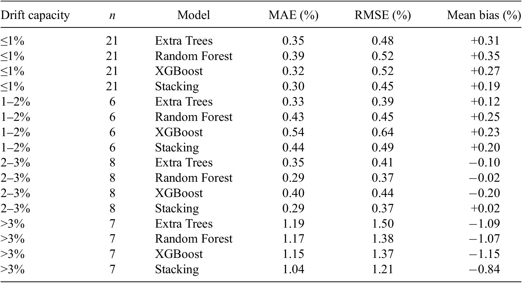
To examine whether the predictive accuracy remained uniform across the observed drift-capacity range, the errors obtained on the independent hold-out subset were further evaluated within four drift-capacity intervals: ≤1%, 1–2%, 2–3%, and >3%. The corresponding results are summarized in Table 3. The test subset contains 21 specimens with drift capacities ≤1%, 6 specimens within 1–2%, 8 specimens within 2–3%, and 7 specimens with drift capacities exceeding 3%. The variation of MAE across the four drift-capacity intervals is illustrated in Figure 5a, while the corresponding mean prediction bias is shown in Figure 5b.
Prediction errors within different drift-capacity intervals on the independent hold-out test subset

Table 3. Long description
The table contains six columns: Drift capacity, n, Model, M A E (%), R M S E (%), and Mean bias (%).
* For Drift capacity less than or equal to 1% (n = 21):
- Extra Trees: M A E 0.35, R M S E 0.48, Mean bias +0.31.
- Random Forest: M A E 0.39, R M S E 0.52, Mean bias +0.35.
- XGBoost: M A E 0.32, R M S E 0.52, Mean bias +0.27.
- Stacking: M A E 0.30, R M S E 0.45, Mean bias +0.19.
* For Drift capacity 1-2% (n = 6):
- Extra Trees: M A E 0.33, R M S E 0.39, Mean bias +0.12.
- Random Forest: M A E 0.43, R M S E 0.45, Mean bias +0.25.
- XGBoost: M A E 0.54, R M S E 0.64, Mean bias +0.23.
- Stacking: M A E 0.44, R M S E 0.49, Mean bias +0.20.
* For Drift capacity 2-3% (n = 8):
- Extra Trees: M A E 0.35, R M S E 0.41, Mean bias -0.10.
- Random Forest: M A E 0.29, R M S E 0.37, Mean bias -0.02.
- XGBoost: M A E 0.40, R M S E 0.44, Mean bias -0.20.
- Stacking: M A E 0.29, R M S E 0.37, Mean bias +0.02.
* For Drift capacity greater than 3% (n = 7):
- Extra Trees: M A E 1.19, R M S E 1.50, Mean bias -1.09.
- Random Forest: M A E 1.17, R M S E 1.38, Mean bias -1.07.
- XGBoost: M A E 1.15, R M S E 1.37, Mean bias -1.15.
- Stacking: M A E 1.04, R M S E 1.21, Mean bias -0.84.
Prediction errors across drift-capacity intervals for the four regression models on the independent hold-out test subset.

Figure 5. Long description
Two side-by-side grouped bar charts labeled a and b. A shared legend at the bottom identifies four models: Extra Trees (dark blue), Random Forest (light blue), XGBoost (dark orange), and Stacking Ensemble (light orange).
Panel a, titled M A E by drift interval:
* The y-axis is M A E in percent, ranging from 0.0 to 1.2.
* The x-axis has four drift-capacity intervals: less than or equal to 1 percent, 1 to 2 percent, 2 to 3 percent, and greater than 3 percent.
* For the first three intervals, M A E remains relatively low, between 0.3 and 0.5 percent.
* In the greater than 3 percent interval, M A E sharply increases for all models to between 1.0 and 1.2 percent.
Panel b, titled Bias by drift interval:
* The y-axis is Bias in percent, ranging from negative 1.2 to 0.4, with a horizontal zero line.
* In the less than or equal to 1 percent and 1 to 2 percent intervals, all models show positive bias between 0.1 and 0.4 percent.
* In the 2 to 3 percent interval, bias fluctuates near zero, with XGBoost showing a negative bias of approximately negative 0.2 percent.
* In the greater than 3 percent interval, all models show a significant negative bias, with Extra Trees, Random Forest, and XGBoost dropping to between negative 1.0 and negative 1.2 percent, while Stacking Ensemble is slightly higher at approximately negative 0.8 percent.
For drift capacities up to 3%, prediction errors remain relatively limited for all four models, although differences among the regressors are observed across the individual intervals. A different behavior is evident for specimens with drift capacities exceeding 3%, where all models exhibit substantially higher MAE and RMSE values and a negative mean bias. This indicates a systematic tendency to underpredict the upper range of drift capacity. The stacking ensemble provides the lowest errors in this interval, with MAE = 1.04% and RMSE = 1.21%, and reduces the magnitude of the mean bias to −0.84%, compared with values ranging from −1.07% to −1.15% for the individual regressors. Nevertheless, the upper-tail underprediction is not eliminated.
This behavior is likely related to the comparatively limited representation of high-drift specimens in the available experimental data. Only 7 of the 42 specimens in the independent test subset exhibit drift capacities above 3%, whereas half of the test specimens have drift capacities ≤1%. Consequently, the models are trained predominantly on lower and moderate drift-capacity responses and have less information available to learn the combinations of geometric, loading, and reinforcement parameters associated with unusually high deformation capacities. The global performance metrics should therefore be interpreted together with the interval-based results, particularly when the models are applied to walls expected to develop large drift capacities.
In addition to the comparison between machine learning models, the predictive performance of the well-known empirical formulation proposed by Abdullah and Wallace (Reference Abdullah and Wallace2019), shown in Equation (4), was evaluated on a subset for which all parameters required by the Abdullah and Wallace formulation were available.

where δc/hw represents the drift capacity, expressed as a percentage; λb is defined as the product of cross-sectional slenderness (lw/b) and compression zone slenderness (c/b); α is the boundary confinement factor (60 for overlapping hoops; 45 for a single perimeter hoop with crossties); ν max is the maximum shear stress, defined as the maximum shear force divided by the effective shear area; and fc′ is the concrete compressive strength.
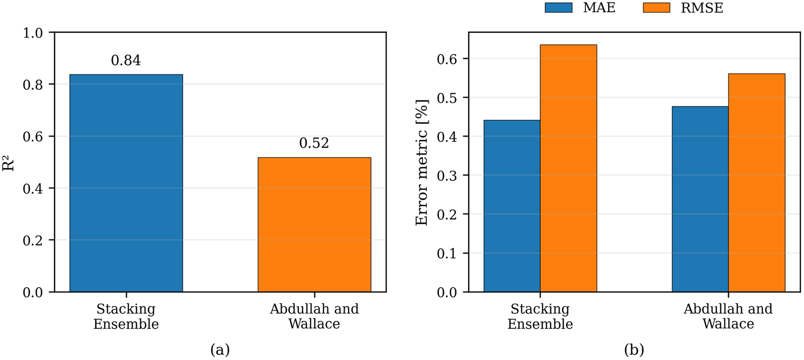
Figure 6 compares the predictive performance of the Stacking Ensemble and the Abdullah and Wallace empirical formula, with the R 2 values presented in Figure 6a and the MAE and RMSE values compared in Figure 6b. The Stacking Ensemble provides a substantially higher coefficient of determination, with R 2 = 0.84 compared with 0.52 for the empirical formulation, and a slightly lower MAE of 0.44% compared with 0.48%. The RMSE values are 0.64% and 0.56%, respectively. The comparison therefore indicates a considerably stronger overall correlation between predicted and experimental drift capacities for the machine learning model, while the error-based metrics remain of comparable magnitude.
Comparison of predictive performance metrics for the Stacking Ensemble and the Abdullah and Wallace empirical formula: (a) predictive accuracy expressed in terms of R 2; (b) prediction errors expressed in terms of MAE and RMSE.

Figure 6. Long description
A multi-panel figure with two side-by-side bar charts labeled a and b.
Panel a is a bar chart showing predictive accuracy. The y-axis is labeled R super 2 with a scale from 0.0 to 1.0. The x-axis lists two models. The Stacking Ensemble model is represented by a blue bar reaching a value of 0.84. The Abdullah and Wallace model is represented by an orange bar reaching a value of 0.52.
Panel b is a grouped bar chart showing prediction errors. The y-axis is labeled Error metric [%] with a scale from 0.0 to 0.6. A legend at the top indicates blue bars represent M A E and orange bars represent R M S E.
* For the Stacking Ensemble model, the blue M A E bar is approximately 0.44 and the orange R M S E bar is approximately 0.63.
* For the Abdullah and Wallace model, the blue M A E bar is approximately 0.48 and the orange R M S E bar is approximately 0.56.
This behavior is further illustrated in Figure 7, which presents the observed versus predicted drift capacity obtained using the Abdullah and Wallace formulation. The predictions obtained with the Stacking Ensemble on the independent hold-out test subset are additionally shown in grey in the background using the same axis limits. The scatter plot shows a noticeable dispersion of the empirical predictions around the ideal diagonal. While the general trend is captured, deviations increase for certain specimens, particularly at higher drift levels.
Observed versus predicted drift capacity using the Abdullah and Wallace formulation, with Stacking Ensemble predictions shown in grey in the background.

Figure 7. Long description
A scatter plot on a grid with the X axis labeled Observed drift capacity [%] and the Y axis labeled Predicted drift capacity [%], both ranging from 0 to 8.
* Statistical Box: Located in the top-left corner, it lists R super 2 = 0.52, M A E = 0.48%, and R M S E = 0.56%.
* Reference Line: A blue dashed diagonal line represents the Ideal prediction where observed equals predicted.
* Data Series:
- Abdullah and Wallace: Represented by red circular markers. These points are concentrated between 1.5 and 4.5 on the X axis, generally following the ideal line but showing a slight under-prediction bias as values increase.
- Stacking Ensemble: Represented by grey circular markers in the background. These points are more widely distributed across the entire range from 0 to 8 on the X axis.
* Trends: Both datasets show a positive linear correlation. The red markers are more tightly clustered around the 2 to 4 percent range, while the grey markers show higher variance, including an outlier near X = 8 and Y = 5.8.
* Legend: Located in the bottom-right corner, identifying the grey dots as Stacking Ensemble, red dots as Abdullah and Wallace, and the blue dashed line as Ideal.
Overall, the substantially higher coefficient of determination obtained by the Stacking Ensemble indicates a closer representation of the observed variability in drift capacity, although the comparison of MAE and RMSE shows that the relative performance of the two approaches also depends on the error metric considered.
6. Conclusion
This study examined the use of tree-based machine learning models for predicting the drift capacity of reinforced concrete shear walls with rectangular and I-shaped cross-sections. A database comprising 208 experimental tests was analyzed using Extra Trees, Random Forest, XGBoost, and a stacking ensemble, with model performance evaluated using nested cross-validation within the development subset followed by a single evaluation on an independent hold-out test subset.
Statistical distributions, scatter plots, and correlation analyses revealed generally weak linear relationships between individual input parameters and drift capacity, confirming that the drift capacity of reinforced concrete shear walls is governed by nonlinear interactions among multiple variables rather than by isolated predictors.
This conclusion becomes clearer when comparing the results with those obtained using the empirical formulation proposed by Abdullah and Wallace. The empirical formulation resulted in a considerably lower R 2 value than the best-performing machine learning model, while the error-based metrics were of comparable magnitude. Although the formulation captures part of the general trend, the substantially higher coefficient of determination obtained by the machine learning approach indicates a better representation of the observed variability in drift capacity. The machine learning models showed good predictive capability on the independent hold-out subset. Among the individual regressors, Random Forest achieved the highest test-set R 2, equal to 0.80, while Extra Trees and XGBoost yielded comparable performance, both reaching R 2 = 0.78. The Stacking Ensemble provided the best overall performance, reaching R 2 = 0.84, MAE = 0.44%, and RMSE = 0.64%. The improvement obtained by combining the individual regressors indicates that, for the present dataset, their complementary predictive patterns can be exploited more effectively than when the models are used independently. A similar benefit of stacking was observed in the authors’ previous study on reinforced concrete columns. However, the fact that the ensemble performs favorably in both applications should not be interpreted as evidence that a single modeling strategy is universally optimal. The relative performance of the individual regressors, the magnitude of the ensemble improvement, and the prediction errors remain dependent on the structural typology, the available predictors, and the statistical characteristics of the experimental database. The interval-based error analysis nevertheless revealed that predictive accuracy is not uniform across the entire drift-capacity range. For specimens with drift capacities exceeding 3%, all considered models exhibited increased errors and a systematic tendency toward underprediction. The Stacking Ensemble reduced this tendency compared with the individual regressors but did not eliminate it. This behavior is associated with the limited representation of high-drift specimens in the available experimental data and indicates that predictions within the upper range should be interpreted with additional caution.
Overall, this study reinforces the potential of machine learning as a complementary data-driven approach to traditional empirical models for drift capacity prediction, while also highlighting the importance of rigorous model validation and adequate representation of the response range in the available experimental data. In this sense, the present work complements the previous study on reinforced concrete columns and provides a consistent framework for understanding how different machine learning approaches perform across different reinforced concrete structural elements. The developed models may support preliminary seismic assessment and performance-based applications in which rapid estimates of wall deformation capacity are required, while detailed structural analysis remains necessary for final design and safety assessment.
Supplementary material
The supplementary material for this article can be found at http://doi.org/10.1017/dce.2026.10080.
Acknowledgments
OpenAI ChatGPT was used during manuscript revision for language editing and improvement of textual clarity. All scientific content was reviewed and approved by the authors, who take full responsibility for the manuscript.
Data availability statement
The experimental data analyzed in this study were derived from the publicly available ACI 445B Shear Wall Database (Pujol et al., Reference Pujol, Song, Wang, Puranam and Usta2019), Version 1.0 (https://doi.org/10.7277/EESD-J453). The processed dataset of 208 specimens, including source identifiers and the fixed development/hold-out assignment used for model evaluation, is openly available on Zenodo (https://doi.org/10.5281/zenodo.22938143) and is also provided as Supplementary Material.
Author contribution
Conceptualization: A.O.K. and I-G.C.; Data curation: A.O.K.; Data visualization: A.O.K.; Formal analysis: A.O.K.; Investigation: A.O.K. and I-G.C.; Methodology: A.O.K. and I-G.C.; Writing—original draft: A.O.K. and I-G.C.; Writing—review and editing: A.O.K. and I-G.C.
Funding statement
There are no funders to report for this submission.
Competing interests
The authors declare none.
Ethical standards
The research meets all ethical guidelines, including adherence to the legal requirements of the study country.






 Open access


Comments
No Comments have been published for this article.