





Impact Statement
This work introduces the Hierarchical Fourier Neural Operator (HFNO) architecture, which decomposes the flow field into multiple spectral scales that are learned and processed independently. This hierarchical treatment of scales significantly reduces model complexity while maintaining predictive accuracy in turbulent flow simulations and providing interpretability across various scales. Compared to standard Fourier Neural Operators, the HFNO achieves comparable statistical performance with five times fewer parameters.
1. Introduction
Modeling high-dimensional dynamical systems governed by partial differential equations (PDEs), such as incompressible fluid flows or reactive transport phenomena, remains a central challenge in scientific computing. These systems exhibit complex nonlinear dynamics and span a broad range of spatial and temporal scales. Accurately resolving all relevant scales requires extremely high resolutions in both space and time, resulting in numerical models that routinely involve billions of degrees of freedom. As a result, high-fidelity simulations—such as Direct Numerical Simulations (DNS; Moin and Mahesh, Reference Moin and Mahesh1998) or Large Eddy Simulations (LES; Piomelli, Reference Piomelli1999)—become prohibitively expensive, particularly at high Reynolds numbers (Pope, Reference Pope2000). Even on modern high-performance computing infrastructures, such simulations often require massive parallelization and remain mostly restricted to limited time horizons or simplified geometries.
Recent advances in neural operator learning have opened new avenues for data-driven surrogate modeling of PDEs. Traditional neural network–based approaches, such as Physics-Informed Neural Networks (PINNs; Raissi et al., Reference Raissi, Perdikaris and Karniadakis2019), model the solution by taking spatial and temporal coordinates as input and enforcing the governing equations through a loss function. While effective for low-dimensional problems, these methods require retraining for each new geometry or discretization, which limits their scalability. More recently, neural operator frameworks have been introduced to learn mappings directly between infinite-dimensional function spaces rather than pointwise quantities. Among them, DeepONet (Lu et al., Reference Lu, Jin and Karniadakis2021) represents an operator using two subnetworks: a branch network sampling the input function at sensor points and a trunk network depending on the output coordinates. Although DeepONet provides theoretical guarantees for a universal operator approximation, its accuracy can be sensitive to the choice and number of sensor points, as well as to the sampling of the training functions.
In contrast, the Fourier Neural Operator (FNO; Li et al., Reference Li, Kovachki, Azizzadenesheli, Liu, Bhattacharya, Stuart and Anandkumar2021) achieves mesh and resolution invariance by parameterizing integral kernels in the Fourier domain. This formulation enables the learned operator to generalize across different discretizations of the same underlying function space, making FNOs particularly attractive for scalable, resolution-independent surrogate modeling of complex dynamical systems (Choubineh et al., Reference Choubineh, Chen, Wood, Coenen and Ma2023; Serrano et al., Reference Serrano, Migus, Yin, Mazari and Gallinari2023; Wang et al., Reference Wang, Li, Yuan, Peng, Liu and Wang2024). Since its introduction, the FNO framework has inspired a wide family of variants, among them the Adaptive FNO (AFNO; Guibas et al., Reference Guibas, Mardani, Li, Tao, Anandkumar and Catanzaro2022) and the Amortized FNO (AM-FNO; Xiao et al., Reference Xiao, Kou, Hao, Lin and Deng2024). Other classes of neural operators have also been developed, such as the Wavelet Neural Operator (WNO; Tripura and Chakraborty, Reference Tripura and Chakraborty2023), which improves multiscale feature representations through localized wavelet bases, and the Graph Neural Operator (GNO; Li et al., Reference Li, Kovachki, Azizzadenesheli, Liu, Bhattacharya, Stuart and Anandkumar2020), which extends operator learning to irregular domains and unstructured meshes. Despite their strong learning capabilities, Fourier Neural Operators (FNOs) remain deep architectures characterized by limited interpretability. Although they embed physical knowledge through the use of Fourier transforms, it is still difficult to assign a clear physical meaning to the learned parameters after training.
This limitation motivates the design of a new architecture, inspired by FNOs, that retains the advantages of a spectral representation while promoting a more interpretable and scale-aware structure. Turbulent flows are inherently multiscale phenomena, characterized by a broad range of interacting spatial and temporal structures. Traditional modeling approaches in fluid mechanics, such as the Reynolds-Averaged Navier–Stokes equations (RANS; Launder and Spalding, Reference Launder and Spalding1974; Pope, Reference Pope2000) and Large-Eddy Simulations (LES; Meneveau and Katz, Reference Meneveau and Katz2000; Pope, Reference Pope2000; Sagaut, Reference Sagaut2006), explicitly exploit this separation of scales to design different modeling strategies for the small- and large-small dynamics—for instance, resolving the energy-containing eddies while modeling the subgrid-scale dynamics. This principle of scale separation has long proven effective in promoting both interpretability and consistency across models operating at different resolutions. Inspired by this idea, the present work aims at designing a neural architecture that can automatically identify and model these scales separately, bridging physical insight from turbulence theory with modern operator-learning techniques. The primary objective of this study is therefore to enforce a clear separation of scales across the parallel layers of the network, both at the input and output levels. This design choice is deliberate, as it enables (i) the explicit reconstruction of the contribution associated with each scale, and (ii) the selective removal of specific wavenumbers when constructing reduced-order representations.
To this end, this contribution introduces the Hierarchical Fourier Neural Operator (HFNO), a novel deep learning architecture inspired by FNOs, designed both to learn mappings between infinite-dimensional function spaces and to decompose predictions across different scales. Our model divides the Fourier domain into disjoint wavenumber bins, each of which is processed by a dedicated Fully Connected Neural Network (FCNN; Hornik et al., Reference Hornik, Stinchcombe and White1989). This approach enables the model to learn scale-specific nonlinear transformations, leading to improved generalization and physical interpretability. A final correction model—implemented as either a CNN (Lecun et al., Reference Lecun, Bottou, Bengio and Haffner1998; Goodfellow et al., Reference Goodfellow, Bengio and Courville2016) or an Echo State Network (Jaeger, Reference Jaeger2010)—further refines the output via residual modeling.
This article is organized as follows. Section 2 presents the general framework of operator learning, with a focus on FNOs. Section 3 introduces the HFNO architecture proposed in this study. Section 4 presents the results of our architecture compared to baseline methods when applied to several cases of variable complexity. Finally, conclusions of the work are discussed in Section 5.
2. Neural operator
In the general case of operator learning, the goal is to learn a mapping between two infinite-dimensional function spaces. Let
$ \mathbf{\mathcal{D}}\subset {\unicode{x211D}}^d $
 be a bounded open set, and let
$ \mathbf{\mathcal{U}}=\mathbf{\mathcal{F}}\left(\mathbf{\mathcal{D}};{\unicode{x211D}}^{d_u}\right) $
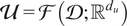 and
$ \mathbf{\mathcal{Y}}=\mathbf{\mathcal{F}}\left(\mathbf{\mathcal{D}};{\unicode{x211D}}^{d_y}\right) $
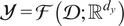 be Banach spaces of functions taking values in
$ {\unicode{x211D}}^{d_u} $
 and
$ {\unicode{x211D}}^{d_y} $
 , respectively. Here, D denotes the subset of the domain where the function is observed, and
$ \mathbf{\mathcal{U}} $
 and
$ \mathbf{\mathcal{U}} $
 represent the input and output function spaces, respectively. The objective is therefore to learn a nonlinear mapping
$ \mathbf{\mathcal{M}}:\mathbf{\mathcal{U}}\to \mathbf{\mathcal{Y}} $
 , which may represent, for example, the solution of a PDE or the evolution of a trajectory, that we usually call an operator.
To this end, we introduce Neural Operators, which are parametric numerical models denoted by
$ {\mathbf{\mathcal{M}}}_{\theta }:\mathbf{\mathcal{U}}\to \mathbf{\mathcal{Y}} $
 . Suppose we are given a dataset of observation pairs
$ {\left({u}_i,{y}_i\right)}_{i=1}^N\in {\left(\mathbf{\mathcal{U}}\times \mathbf{\mathcal{Y}}\right)}^N $
 , such that
$ {y}_i=\mathbf{\mathcal{M}}\left({u}_i\right) $
 . The goal is to find parameters
$ \theta $
 such that
$ {\mathbf{\mathcal{M}}}_{\theta } $
 approximates the true operator M as accurately as possible, in the sense of minimizing a cost functional
$ J:\mathbf{\mathcal{Y}}\times \mathbf{\mathcal{Y}}\to {\unicode{x211D}}_{+} $
 . This setup defines a supervised learning problem.
In the present case, the function spaces involved are continuous. To enable numerical treatment, the domain D is discretized using a Cartesian mesh. Functions
$ u\in \mathbf{\mathcal{U}} $
 or
$ y\in \mathbf{\mathcal{Y}} $
 are then represented by their evaluations at a set of points
$ \mathbf{\mathcal{G}}={\left({\mathbf{x}}_j\right)}_{j=1}^n\subset \mathbf{\mathcal{D}} $
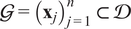 , which sample the domain
$ \mathbf{\mathcal{D}} $
 . For a Cartesian mesh, we typically define
$ {n}_k $
 as the number of discretization points along each dimension
$ k\in \left\{1,\dots, d\right\} $
 , so that the total number of grid points is given by
$ n={\prod}_k{n}_k $
 . The coordinates of the grid points in each dimension are specified by vectors
$ {x}^{(k)}\in {\unicode{x211D}}^{n_k} $
 . Thus, any grid point can be identified by its multi-index
$ \left({i}_1,\dots, {i}_d\right)\in \left\{1,\dots, {n}_1\right\}\times \cdots \times \left\{1,\dots, {n}_d\right\} $
 .
In most cases, the learning process depends on the chosen discretization, and the evaluation of solutions is restricted to the discrete points
$ {\mathbf{x}}_j $
 , as is the case with DeepONets (Lu et al., Reference Lu, Jin and Karniadakis2021). These points are commonly referred to as sensors. As we will see later, the use of the Fourier transform helps mitigate this dependence on specific sensor locations, enabling the design of mesh-invariant solvers.
One architecture that has shown remarkable performance and impact in recent years is the Fourier Neural Operator (FNO, Li et al., Reference Li, Kovachki, Azizzadenesheli, Liu, Bhattacharya, Stuart and Anandkumar2021). This architecture is defined iteratively through a sequence of mappings
$ {v}_0\mapsto {v}_1\mapsto \dots \mapsto {v}_T $
 , where
$ {v}_j\in \mathbf{\mathcal{F}}\left(\mathbf{\mathcal{D}};{\unicode{x211D}}^{d_v}\right) $
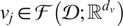 . The input field u is first lifted to a higher-dimensional representation by a local transformation P, such that
$ \forall x,{v}_0(x)=P\left(u(x)\right) $
 . The lifting operator P is typically implemented as a shallow, fully connected neural network (FCNN). Each transformation
$ {v}_t\mapsto {v}_{t+1} $
 , referred to as a Fourier layer, is defined as:

where
$ \sigma $
 is a nonlinear activation function (typically a
$ \tanh $
 or ReLU),
$ {W}_t\in {\unicode{x211D}}^{d_v\times {d}_v} $
 is a local linear transformation, and
$ {K}_t $
 is an integral operator acting on the functional space
$ \mathbf{\mathcal{F}}\left(\mathbf{\mathcal{D}};{\unicode{x211D}}^{d_v}\right) $
 , defined by

where
$ \mathcal{F} $
 and
$ {\mathbf{\mathcal{F}}}^{-1} $
 denote the Fourier and inverse Fourier transforms, respectively. The tensor
$ {R}_t $
 parametrizes the operator
$ {K}_t $
 and is defined by
$ {R}_t(k)\in {\unicode{x2102}}^{d_v\times {d}_v} $
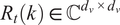 . To better understand Equation 2.2, we can write explicitly

which shows that the operation consists of a channel-wise multiplication in Fourier space. Finally, the output of the last layer
$ {v}_T $
 is projected onto the output space through another shallow FCNN
$ Q $
 , yielding the final output
$ y(x)=Q\left({v}_T(x)\right) $
 . The reader is referred to the original article (Li et al., Reference Li, Kovachki, Azizzadenesheli, Liu, Bhattacharya, Stuart and Anandkumar2021) for more information regarding the details of the procedure.
As mentioned previously, a key advantage of the FNO architecture lies in its mesh invariance: the operator acts globally over the entire spatial domain rather than locally on discrete points. All operations are either performed in physical space—independent of the specific spatial coordinates—or in Fourier space, where the low-frequency Fourier coefficients remain consistent across discretizations that satisfy the Nyquist–Shannon sampling criterion.
3. Hierarchical Fourier Neural Operator
The Hierarchical Fourier Neural Operator (HFNO) operates on a latent space that differs from that of a classical autoencoder or a variational autoencoder (Hinton and Salakhutdinov, Reference Hinton and Salakhutdinov2006; Kingma and Welling, Reference Kingma and Welling2022); instead, the latent space is defined in the Fourier domain to exploit physical structure, particularly in periodic problems. This choice not only aligns with the underlying structure of periodic problems but also guarantees exact and lossless reconstruction of signals via analytically defined Fourier transform and inverse Fourier transform operations. In addition, the architecture treats the scales separately by performing a different transformation for different ranges of Fourier coefficients. The aim is to learn how to model phenomena specific to each range of scales, and to reduce the complexity of each component’s task.
Beyond its spectral formulation, the HFNO remains intrinsically meshless. It operates independently of spatial discretization and is thus adaptable to complex or irregular geometries. Although its design naturally aligns with periodic problems, several extensions have demonstrated its ability to handle nonperiodic boundary conditions effectively (Li et al., Reference Li, Kovachki, Azizzadenesheli, Liu, Bhattacharya, Stuart and Anandkumar2021; Pathak et al., Reference Pathak, Subramanian, Harrington, Raja, Chattopadhyay, Mardani, Kurth, Hall, Li, Azizzadenesheli, Hassanzadeh, Kashinath and Anandkumar2022; Kovachki et al., Reference Kovachki, Li, Liu, Azizzadenesheli, Bhattacharya, Stuart and Anandkumar2024).
The architecture proposed in this work is divided into two components: (i) the spectral block, which processes low-frequency modes grouped into blocks of submodes and predicts coarse-scale behavior, and (ii) the residual block, which processes the remaining modes in order to predict a correction term, that is, a residual closure. The second component will be discussed for different design choices. A visualization of the generic HFNO architecture is shown in Figure 1. Each component will be further described in what follows.
Generic HFNO architecture proposed in this work.

Figure 1. Long description
The flowchart begins on the far left with input u of x, represented by three vertical white rectangles. A green arrow labeled P points to a second set of blue rectangles labeled a of x. A second green arrow labeled F F T points to a grid-like blue structure labeled a hat of k.
From a hat of k, the data splits into three paths:
1. The top path leads to a set of blue rectangles with a spiral icon above them, entering a green box containing a neural network diagram with nodes and connections. This is labeled open parenthesis A sub l close parenthesis super p with l equals 1. The output passes through yellow rectangles to a yellow grid labeled a double-hat of k.
2. The middle path mirrors the top path, entering a second green neural network box labeled open parenthesis A tilde sub l close parenthesis super p with l equals 1, also feeding into the yellow grid a double-hat of k.
3. The bottom path branches from the initial a hat of k to a label Last modes a sub res of x, which enters a green box labeled Residual Predictor.
On the right side, the yellow grid a double-hat of k passes through a red arrow labeled I F F T to become red rectangles labeled a tilde of x. Simultaneously, the Residual Predictor outputs red rectangles labeled a tilde sub res of x. Both red data streams converge at a green circle containing a plus sign. The final output, y tilde, is represented by three red rectangles on the far right.
3.1. Spectral block
As in the case of the FNO, we first apply a lifting layer P that projects the input u into a higher-dimensional space, yielding
$ a\in \mathbf{\mathcal{F}}\left(\mathbf{\mathcal{D}};{\unicode{x211D}}^{d_a}\right) $
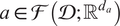 with
$ {d}_a>{d}_u $
 , such that
$ \forall x\in \mathbf{\mathcal{D}},a(x)=P\left(u(x)\right) $
 . The lifting operator P is typically implemented as a shallow Fully Connected Neural Network (FCNN) without nonlinear activation, which amounts to a linear transformation from
$ {\unicode{x211D}}^{d_u} $
 to
$ {\unicode{x211D}}^{d_a} $
 .
The function
$ x\mapsto a(x) $
 is then transformed into the frequency domain using a Fast Fourier Transform (FFT) over the spatial variable
$ x\in \mathbf{\mathcal{D}} $
 . Using the previously introduced Cartesian grid notation, we numerically obtain
$ \hat{a} $
 , the Fourier representation of
$ a $
 , defined by
$ \mathbf{k}\mapsto \hat{a}\left(\mathbf{k}\right)\in {\unicode{x2102}}^{d_a} $
 for
$ \mathbf{k}\in {\mathrm{\mathbb{Z}}}^d $
 . The frequency modes k are then partitioned into blocks. We select a sequence of positive real numbers
$ 0={c}_0<{c}_1<\dots <{c}_p $
 , and define the
$ l $
 -th block of modes by

The choice of norm
$ \parallel \cdot \parallel $
 is arbitrary, but the
$ {\mathrm{\ell}}_2 $
 -norm is typically used in practice. Examples of partitioning strategies are shown in Figure 2. Since we use an increasing sequence of thresholds to define the blocks, each block corresponds to a range of modes associated with progressively finer scales. This construction enables a flexible separation of scales, where the thresholds
$ {c}_l $
 act as hyperparameters of the model.
Three different partitioning strategies are shown from left to right: based on the
$ {L}_2 $
 -norm, the
$ {L}_{inf} $
 norm, and a semi-norm depending on a single axis.
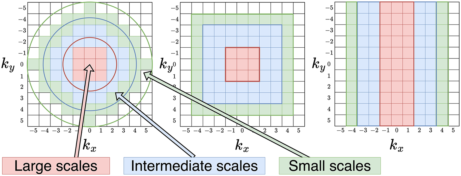
Figure 2. Long description
The figure consists of three panels, each featuring a 10 by 10 grid with axes labeled k sub x and k sub y ranging from negative 5 to 5.
In the first panel, the partitioning is circular. At the center, a red circle encloses a 3 by 3 block of red-shaded cells labeled Large scales. Moving outward, a blue ring encloses a larger area of blue-shaded cells labeled Intermediate scales. The outermost layer is a green circle enclosing green-shaded cells labeled Small scales.
In the second panel, the partitioning is square-shaped. The innermost region is a red 3 by 3 square. This is surrounded by a larger blue square frame, which is in turn enclosed by a green square frame at the perimeter.
In the third panel, the partitioning is based on vertical bands along the k sub x axis. The central band from k sub x equals negative 1 to 1 is shaded red. Flanking this are two blue bands from negative 3 to negative 2 and 2 to 3. The outermost bands from negative 5 to negative 4 and 4 to 5 are shaded green.
Three color-coded labels at the bottom point to their respective regions across the panels. A red box labeled Large scales points to the center. A blue box labeled Intermediate scales points to the middle layer. A green box labeled Small scales points to the outer layer.
The Fourier-transformed function
$ \hat{a} $
 can now be divided into bins of Fourier modes according to the previously defined partitioning of Fourier space. These are defined as
$ {\mathbf{\mathcal{A}}}_l=\left\{\hat{a}\left(\mathbf{k}\right)|\mathbf{k}\in {\mathbf{\mathcal{K}}}_l\right\} $
 for
$ l\in \left\{1,\dots, p\right\} $
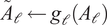
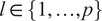 . A nonlinear transformation is then applied independently to each of these bins, within a space that preserves the same Fourier modes but maps them to a new function valued in the output space. Concretely, each bin is flattened into a C-valued vector of size
$ {s}_l=\operatorname{card}\left({\mathbf{\mathcal{K}}}_l\right)\cdot {d}_a $
 and is mapped to a C-valued vector of size
$ {q}_l=\operatorname{card}\left({\mathbf{\mathcal{K}}}_l\right)\cdot {d}_y $
 using a mapping
$ {g}_l:{\unicode{x2102}}^{s_l}\to {\unicode{x2102}}^{q_l} $
 . We choose these mappings to be fully connected neural networks (FCNNs), for which we can configure hyperparameters such as depth and width. By allowing each mapping to be tuned independently, we can assign greater representational capacity to specific bins as needed. The output of each transformation now represents a bin of Fourier modes of a new function
$ \tilde{a} $
 , following the same partitioning used previously. We define this as
$ {\tilde{\mathbf{\mathcal{A}}}}_l=\left\{\hat{\tilde{a}}\left(\mathbf{k}\right)|\mathbf{k}\in {\mathbf{\mathcal{K}}}_l\right\} $
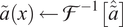
 . These bins are then aggregated using the inverse of the partitioning mapping, resulting in the complete Fourier representation of
$ \tilde{a} $
 . We finally inverse-Fourier transform using an IFFT to revert into the output space to obtain
$ \tilde{a} $
 that will be the first part of the output, representing the lowest scales of the prediction. In the following, we refer to each scale-independent transform as a “Fourier layer.”
As mentioned previously, this architecture is particularly well suited for periodic problems. However, it is possible to extend its applicability to non-periodic signals using the padding strategy. This involves applying zero-padding to the input signal, effectively enlarging the domain by adding zeros around the original data. By doing so, the signal can be treated as approximately periodic within the extended domain, enabling the model to exploit the Fourier-based latent space while mitigating boundary artifacts.
An important distinction between HFNO and FNO lies in the placement of activation functions, which play a crucial role in deep learning architectures by enhancing their expressive power. In the case of HFNO, activation functions are applied directly in the Fourier domain. This design choice enables the model to produce outputs that are naturally separated, interpretable, and additive, as each intermediate mapping directly corresponds to the Fourier transform of the final layer output. Indeed, representing a function in the Fourier domain is equivalent to representing it in the physical domain, since the Fourier transform is a bijective mapping, and therefore, this choice should not fundamentally alter the model’s learning capabilities.
3.2. Residual block
The second part of the architecture serves as a residual corrector targeting the finest scales. We explore two different approaches. The first applies corrections directly in physical space, rather than in Fourier space as done in the previous stage. The second employs a Recurrent Neural Network (RNN) in Fourier space to incorporate memory and enhance the model’s ability to capture high-frequency components more effectively.
3.2.1. Prediction in physical space
The goal is to apply a transformation in physical space to account for the scales not handled by the first part of the model. To do so, we extract the Fourier modes that were not included in the previous partitioning, up to a user-defined threshold
$ {c}_{max} $
 . These modes define an additional block in the partition, given by
$ {\mathbf{\mathcal{K}}}_{res}=\left\{\mathbf{k}\in {\mathrm{\mathbb{Z}}}^d|{c}_p\le \parallel \mathbf{k}\parallel <{c}_{max}\right\} $
 . We thus consider a truncated version of
$ \hat{a} $
 defined as
$ {\hat{a}}_{res}:{\mathbf{\mathcal{K}}}_{res}\to {\unicode{x2102}}^{d_a} $
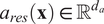
 . This representation is brought back to physical space via the inverse Fourier transform, yielding
$ {a}_{res} $
 with values in
$ {\unicode{x211D}}^{d_a} $
 , that is,
$ {a}_{res}\left(\mathbf{x}\right)\in {\unicode{x211D}}^{d_a} $
 .
The final step consists of mapping this latent-space representation to the output space. This transformation is of the form
$ \mathbf{\mathcal{W}}:\mathbf{\mathcal{F}}\left(\mathbf{\mathcal{D}};{\unicode{x211D}}^{d_a}\right)\to \mathbf{\mathcal{F}}\left(\mathbf{\mathcal{D}};{\unicode{x211D}}^{d_y}\right) $
 . We investigate two types of transformations. The first is a simple linear map
$ W:{\unicode{x211D}}^{d_a}\to {\unicode{x211D}}^{d_y} $
 , constant in space, such that
$ \forall x\in \mathbf{\mathcal{D}},{Wa}_{res}(x)={\tilde{a}}_{res}(x) $
 . Due to its limited expressiveness, we also explore a more flexible model based on a Convolutional Neural Network (CNN), which operates directly on the full field
$ {a}_{res} $
 rather than pointwise on
$ {a}_{res}(x) $
 .
Finally, the two contributions are summed to produce the final prediction:
$ \tilde{y}=\tilde{a}+{\tilde{a}}_{\mathrm{res}} $
 . The complete process is described in Algorithm 1.
Algorithm 1 HFNO with Residual Prediction
Require: Input field
$ u(x) $
 on domain
$ D $

Ensure: Prediction
$ \tilde{y}(x) $

1: Lifting:
$ a(x)\leftarrow P\left(u(x)\right) $

2: FFT:
$ \hat{a}(k)\leftarrow \mathbf{\mathcal{F}}\left[a(x)\right] $

3: Partition Fourier modes: define
$ {\left({K}_{\mathrm{\ell}}\right)}_{\mathrm{\ell}=1}^p $

4: for
$ \mathrm{\ell}=1 $
 to
$ p $
 do
5: Extract bin
$ {A}_{\mathrm{\ell}}=\left\{\hat{a}(k)\;|\;k\in {K}_{\mathrm{\ell}}\right\} $

6: Flatten
$ {A}_{\mathrm{\ell}} $
 into vector
7: Apply nonlinear map
$ {\tilde{A}}_{\mathrm{\ell}}\leftarrow {g}_{\mathrm{\ell}}\left({A}_{\mathrm{\ell}}\right) $
8: end for
9: Reconstruction in Fourier space: assemble
$ \hat{\tilde{a}} $
 from
$ \left({\tilde{A}}_{\mathrm{\ell}}\right) $

10: IFFT:
$ \tilde{a}(x)\leftarrow {\mathbf{\mathcal{F}}}^{-1}\left[\hat{\tilde{a}}\right] $
11: Residual modes: define
$ {K}_{\mathrm{res}} $

12: Extract
$ {\hat{a}}_{\mathrm{res}}(k) $
 for
$ k\in {K}_{\mathrm{res}} $

13:
$ {a}_{\mathrm{res}}(x)\leftarrow {\mathbf{\mathcal{F}}}^{-1}\left[{\hat{a}}_{\mathrm{res}}\right] $

14: Residual mapping:
15: either
$ {\tilde{a}}_{\mathrm{res}}(x)\leftarrow W\left({a}_{\mathrm{res}}(x)\right) $
 (linear)
16: or
$ {\tilde{a}}_{\mathrm{res}}(x)\leftarrow \mathrm{CNN}\left({a}_{\mathrm{res}}(x)\right) $

17: Output:
$ \tilde{y}(x)\leftarrow \tilde{a}(x)+{\tilde{a}}_{\mathrm{res}}(x) $

3.2.2. Prediction in wave-number space
Echo State Networks (ESNs, Jaeger, Reference Jaeger2010) are a specific class of Recurrent Neural Networks (RNNs) belonging to the reservoir computing paradigm. They seek to simplify the training of recurrent architectures while preserving their capability to model complex temporal dynamics. Unlike traditional RNNs, where all recurrent weights are trained, ESNs employ a large, randomly connected, and fixed recurrent layer known as the reservoir. Only the output connections are learned, resulting in efficient and numerically stable training. ESNs have been widely employed in the scientific community to predict dynamical trajectories, both in full and reduced-order spaces (Heyder and Schumacher, Reference Heyder and Schumacher2021; Özalp and Magri, Reference Özalp and Magri2025). Their proven ability to capture complex temporal dependencies motivates their consideration for future extensions of the proposed model, particularly in the context of predicting dynamical trajectories.
An ESN is composed of three key components, illustrated in Figure 3: an input layer, which projects the external input signal into the high-dimensional reservoir space; a reservoir, that is, a sparsely connected recurrent network providing rich nonlinear dynamics; and an output layer, which linearly combines the reservoir states to generate the network output.
Architecture of an Echo State Network (ESN).

Let
$ \mathbf{u}(t)\in {\unicode{x211D}}^{N_u} $
 denote the input vector at time step
$ t $
 ,
$ \mathbf{x}(t)\in {\unicode{x211D}}^{N_x} $
 the reservoir state vector, and
$ \mathbf{y}(t)\in {\unicode{x211D}}^{N_y} $
 the output vector. The ESN dynamics are governed by the following discrete-time equations:


where
-
• $ {W}_{\mathrm{in}}\in {\unicode{x211D}}^{N_x\times {N}_u} $
 is the input weight matrix,
-
• $ W\in {\unicode{x211D}}^{N_x\times {N}_x} $
is the recurrent (reservoir) weight matrix, -
• $ {W}_{\mathrm{fb}}\in {\unicode{x211D}}^{N_x\times {N}_y} $
is an optional feedback matrix, -
• $ {W}_{\mathrm{out}}\in {\unicode{x211D}}^{N_y\times \left({N}_x+{N}_u+1\right)} $
is the trainable output matrix, -
• $ f\left(\cdot \right) $
is a nonlinear activation function, typically
$ \tanh $
, -
• $ \alpha $
is the leaking rate.






During training, the internal weights (
$ {W}_{\mathrm{in}} $
 ,
$ W $
 ,
$ {W}_{\mathrm{fb}} $
 ) remain fixed, while
$ {W}_{\mathrm{out}} $
 is optimized using linear or ridge regression to minimize the prediction error. The matrices
$ {W}_{\mathrm{in}} $
 and
$ W $
 are typically initialized randomly, with
$ {W}_{\mathrm{in}} $
 that can be either dense or sparse and
$ W $
 sparse (Lukoševičius, Reference Lukoševičius, Montavon, Orr and Müller2012).
The reservoir acts as a nonlinear dynamical system that maps the input sequence into a high-dimensional state space. Its key property, the echo state property (ESP), ensures that the influence of past inputs on the current state vanishes over time. Formally, the ESP requires that, for any bounded input sequence
$ \left\{\mathbf{u}(t)\right\} $
 , the difference between two state trajectories
$ {\mathbf{x}}_1(t) $
 and
$ {\mathbf{x}}_2(t) $
 , initialized differently but driven by the same input, converges to zero as
$ t\to \infty $
 . A sufficient (though not necessary) condition for the ESP is that the spectral radius
$ {\rho}_{spectral}(W) $
 of the reservoir weight matrix satisfies

which guarantees that the internal dynamics are contractive and stable. ESNs thus provide an efficient and robust framework for modeling temporal and sequential data. Their main advantages include fast training, numerical stability, and the ability to capture complex temporal dependencies through high-dimensional nonlinear reservoir dynamics. They have been successfully applied to time-series prediction, signal processing, system identification, and control tasks.
Echo State Networks (ESNs) are particularly well suited for low-dimensional data, meaning that the input and output spaces, where u and y lie, should have relatively small dimensions. This is because the expressive power of ESNs relies on the large size of the reservoir compared to the input and output spaces. Moreover, the trainable parameters are obtained through a least-squares optimization, whose computational complexity grows linearly with the output dimension. For this reason, ESNs cannot be applied directly in the physical space, which typically involves an extremely high number of degrees of freedom, often reaching billions in practical fluid dynamics problems. A reduced representation of the data is thus required. Following the methodology introduced in the previous section, the Fourier transform of the physical-space data provides a suitable reduced representation. Consequently, we use the remaining high-frequency modes—those not already employed in the Fourier layers—as the input for the ESN residual predictor.
3.3. Training process
Regarding the different nature of the two architectures, we adopt distinct training procedures for each. In both cases, the cost functional
$ \mathbf{\mathcal{J}} $
 is defined as the
$ {L}^2 $
 -norm integrated over the domain
$ \mathbf{\mathcal{D}} $
 . Given two fields
$ y $
 and
$ \tilde{y} $
 , the loss is expressed as

where
$ \parallel \cdot \parallel $
 denotes the Euclidean norm in the codomain of
$ y, $
 and
$ \left|\mathbf{\mathcal{D}}\right| $
 stands for the volume of
$ \mathbf{\mathcal{D}} $
 .
Due to the limited number of trainable parameters in the ESN and the linearity of its output layer, training can be efficiently performed using a least-squares approach, which is both faster and more accurate than the gradient-based methods commonly employed in standard deep learning models. Consequently, the residual component is trained separately using the ESN. In cases where the ESN is not used, all model components are trained jointly in an end-to-end manner.
In cases where the residual corrector is either linear or implemented as a CNN, we are given a dataset of input/output pairs
$ {\left({u}_j,{y}_j\right)}_{j=1}^{N_{data}} $
 and aim to approximate the operator M mapping u to y using a parameterized model
$ {\mathbf{\mathcal{M}}}_{\theta } $
 , constructed as previously described. The objective is to minimize the loss
$ {\sum}_j\mathbf{\mathcal{J}}\left({y}_j,{\mathbf{\mathcal{M}}}_{\theta}\left({u}_j\right)\right) $
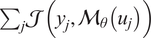 over the parameter space of
$ \theta $
 . The model was trained using the Adam optimizer, which belongs to the family of stochastic gradient-based optimization methods.
In the case where the residual corrector is an ESN, the training procedure differs slightly. Let
$ {\mathbf{\mathcal{M}}}^{spec} $
 denote the spectral binned component of the model, and
$ {\mathbf{\mathcal{M}}}^{res} $
 the residual correction component. We first train
$ {\mathbf{\mathcal{M}}}^{spec} $
 by minimizing the cost functional. Once trained, we use it to compute predictions
$ {y}_{pred,j}={\mathbf{\mathcal{M}}}^{spec}\left({u}_j\right) $
 . The ESN-based corrector
$ {\mathbf{\mathcal{M}}}^{res} $
 is then trained to predict the residual
$ {y}_j-{y}_{pred,j} $
 using the ESN training procedure.
4. Results
Results are presented for three distinct cases, each selected to reflect varying levels of complexity and application objectives. The first case involves the Kuramoto–Sivashinsky (KS) equation, providing a simplified scenario that facilitates a baseline comparison of the proposed method. In the second case, involving the Kolmogorov flow, the model is employed as an emulator to predict subsequent snapshots in a time-resolved sequence, thereby demonstrating the suitability of Echo State Networks (ESNs) for temporal forecasting tasks. The model’s sole purpose is to predict the mapping from the current snapshot to the next; it is not used in an autoregressive fashion. Finally, in the turbulent channel flow case, the model is utilized to map filtered data from an off-wall plane to wall shear stress, serving as an a priori test for wall model implementations in large-eddy simulations.
4.1. Kuramoto–Sivashinsky equation
We first evaluate our model on the one-dimensional Kuramoto–Sivashinsky (KS) equation, a standard benchmark in nonlinear dynamics due to its ease of numerical simulation and its rich nonlinear behavior. The KS equation is formulated as follows:

where L denotes the length of the one-dimensional domain, v controls the dissipative properties of the system, and g represents the prescribed initial condition. The first equation can be reorganized as

where

is the material derivative. Our objective is to predict the material derivative as a function of u. In particular, we seek to learn the operator

which is a linear operator parameterized by v.
To generate the datasets, 10 numerical simulations of the Kuramoto–Sivashinsky (KS) equation are performed using different initial conditions. The first eight trajectories are used for training and the last two remaining for testing. The initial conditions are periodic signals that are represented as weighted sums of sine and cosine functions, and different simulations are generated by varying these coefficients. The spatial domain is defined by
$ L=22 $
 , and the viscosity parameter is set to
$ \nu =0.7 $
 . Each simulation produces a trajectory consisting of
$ {N}_t=2000 $
 temporal snapshots on a spatial grid with
$ {n}_x=1024 $
 points. The system is spatio-temporally chaotic with a Lyapunov exponent
$ \lambda \approx 0.08 $
 and a Lyapunov time
$ {t}_l\approx 12.5 $
 computed as recommended in Edson et al. (Reference Edson, Bunder, Mattner and Roberts2019). In all the figures presented in the following, we non-dimensionalize the time using
$ {t}_l $
 .
We employ an HFNO architecture composed of two parallel Fourier layers coupled with a linear residual predictor. The architectural design, particularly the number of layers and the allocation of Fourier modes, is treated as a hyperparameter optimization problem, where model capacity must be carefully balanced against performance degradation. Empirical observations indicate that, beyond an optimal depth, increasing the number of layers leads to a decline in predictive accuracy. This behavior is attributed to the progressive loss of effective intermodal interactions, which disrupts the underlying dependencies governing the flow dynamics, as shown in Appendix A.
Accordingly, a two-layer configuration is retained as it provides an effective compromise between scale separation and overall model performance. In this setting, the first 16 Fourier modes are considered and partitioned between the two layers: the first layer processes the lowest 6 modes, while the second handles the remaining 10. This choice is guided by the observed elbow in Figure 4, where a separation at mode 6 yields a favorable trade-off between minimizing error and preserving coherent groupings of modes. Each Fourier layer is parameterized by a multilayer perceptron composed of two fully connected layers with 64 neurons and GeLU activation functions, and the lifting dimension is fixed at 64. The remaining architectural details are provided in Appendix A, along with those of the FNO architecture used as a baseline for comparison.
Relative MSE depending on the separation mode for two-layer HFNO models. The red dot indicates the number of modes used in the selected architecture.

Figure 4. Long description
The horizontal X axis is labeled Layer configuration (k underscore sep, 16) with integer markers from 1 to 15. The vertical Y axis is labeled Relative error (%) with markers from 4 to 8.
Data points are connected by a blue line.
* From x equals 1 to 4, the error slightly decreases from approximately 3.8 to a minimum of 3.4.
* At x equals 6, a data point is highlighted with a red circle at approximately 3.7 percent error.
* From x equals 6 to 7, there is a sharp increase to nearly 5 percent.
* The error remains stable at x equals 8 before rising steeply to a peak of approximately 7.9 percent at x equals 13.
* After x equals 13, the error drops sharply to approximately 5.8 percent at x equals 15.
The trained HFNO model is subsequently evaluated against a standard FNO baseline using relative root mean square error (RMSE) and relative mean absolute error (MAE) metrics, along with model size, as summarized in Table 1. The results indicate that the HFNO exhibits slightly higher prediction errors compared to the baseline, which is consistent with its deliberately shallow architecture. Nevertheless, this reduction in depth yields a substantial decrease in the number of parameters and, more importantly, enables a clearer interpretation of scale-dependent contributions to the flow representation. These properties provide a meaningful trade-off, where improved efficiency and interpretability offset the modest loss in predictive accuracy.
KS equation: comparison between FNO and HFNO in terms of relative errors and number of parameters

Table 1. Long description
The table consists of three columns and four rows. The columns are labeled F N O and H F N O.
* The first row shows Relative R M S E in percent. F N O has a value of 1.54 and H F N O has a value of 3.70.
* The second row shows Relative M A E in percent. F N O has a value of 1.20 and H F N O has a value of 3.61.
* The third row shows the Number of parameters. F N O has 850k parameters while H F N O has 36k parameters.
Figure 5 shows the model predictions in a spatiotemporal representation, compared to the ground truth. The corresponding error field is also reported. The last three plots show the contributions of each component of the architecture to the final prediction. As expected, the first Fourier layer predominantly captures the large-scale structures, the second layer resolves the smaller-scale features, while the residual predictor accounts for the remaining discrepancies.
KS equation: contour plots of
$ \frac{Du}{Dt} $
 .

Figure 5. Long description
A six-panel grid of contour plots. All plots share an x-axis from 0.0 to 11.2 and a y-axis from 0 to 20.
* Panel a, Target flow. Shows wavy horizontal bands of red (positive) and blue (negative) values ranging from -5 to 5. The bands exhibit periodic oscillations and downward shifts.
* Panel b, Contribution of first Fourier layer. Displays a similar wavy pattern but with a smaller magnitude range from -1 to 1, showing more diffuse color gradients.
* Panel c, Prediction. Visually identical to panel a, showing the model’s reconstruction of the target flow with a scale of -5 to 5.
* Panel d, Contribution of second Fourier layer. Shows high-frequency oscillations within the wavy bands, with a magnitude scale of -5 to 5, capturing finer structural details than the first layer.
* Panel e, Absolute value of total error. A dark plot using a purple-to-yellow scale from 0.0 to 0.4. Most of the area is dark purple (low error), with thin vertical streaks of yellow indicating localized discrepancies.
* Panel f, Contribution of linear residual predictor. Shows very fine, dense vertical oscillations across the entire domain with a small magnitude range from -0.1 to 0.1.
In order to provide further context, Figure 6 presents the phase-space density in the (
$ {u}_x $
 –
$ {u}_{xx} $
 ) plane, illustrating the distribution of states for both the ground truth and the predictions from different models. Each subplot corresponds to the trajectory in phase space as reconstructed by the respective model. We observe that the first Fourier layer, which represents the low-wavenumber modes, captures the densest regions of the plane. Incorporating the second layer and the residual predictor progressively refines this distribution, resulting in a phase-space representation that more closely resembles the ground truth.
KS equation: density plot in the (
$ {u}_x $
 -
$ {u}_{xx} $
 ) phase plane for different predictions.

Figure 6. Long description
A four-panel density plot series. Each panel shares the same axes. The horizontal x-axis is u sub x ranging from negative 10 to 6. The vertical y-axis is u sub x x ranging from negative 20 to 20. A logarithmic color scale on the right of each plot indicates density from 10 super 1 to 10 super 3 using a purple to yellow gradient.
* Panel a, Ground truth. Shows a complex, crescent-shaped distribution with a dense yellow core at u sub x equals 2 and u sub x x equals 0. A secondary outer ring of lower density purple points extends from u sub x equals negative 10 to 2.
* Panel b, First layer only. Displays a very limited, small elliptical cluster centered at u sub x equals 0 and u sub x x equals 0. It lacks the outer structure seen in the ground truth.
* Panel c, First two layers. Shows a significant increase in complexity compared to panel b. It captures the central dense core and a partial crescent shape, though the outer edges are less defined than the ground truth.
* Panel d, Full model. Closely resembles the ground truth in panel a. It shows the full crescent distribution and the dense central core, indicating high predictive accuracy for the complete model.
To complement these results, Figure 7 shows the energy spectrum of the Kuramoto–Sivashinsky test trajectory, together with the energy spectra predicted by each component of the model (the two Fourier layers and the linear residual predictor). As illustrated, each Fourier layer primarily reconstructs the flow features within its targeted spectral range, effectively capturing the corresponding structures at those characteristic scales. Notably, the residual predictor also contributes to these modes; although it is slightly less accurate than the Fourier layers, it successfully recovers the high-wavenumber portion of the energy spectrum, ensuring a faithful representation of the smaller-scale dynamics. These observations substantiate that the HFNO architecture achieves the intended scale separation: different layers operate on complementary regions of the energy spectrum, collectively enabling an accurate multi-scale representation of the chaotic flow dynamics.
KS equation: energy spectrum of the reference solution and the contributions of each component of the model. The spectra corresponding to the ground truth, the first Fourier layer, the second Fourier layer, and the linear residual predictor are displayed in black, red, blue, and orange, respectively.

Figure 7. Long description
The x-axis represents Wavenumber k Spatial mode on a logarithmic scale from 10 super 0 to approximately 5 times 10 super 1. The y-axis represents Energy E k on a logarithmic scale from 10 super -14 to 10 super 0.
* The ground truth reference solution is a solid black line that rises from 10 super -3 at k equals 1, peaks near 10 super -1 between k equals 5 and 10, and then decays sharply toward 10 super -14 as k approaches 40.
* The first Fourier layer, shown as a dashed red line, perfectly overlaps the ground truth from k equals 1 to approximately k equals 6, where it then drops vertically toward 10 super -14.
* The second Fourier layer, shown as a dashed blue line, rises sharply from 10 super -14 at k equals 5 to meet the ground truth peak, overlapping it until approximately k equals 15, where it then drops vertically.
* The linear residual predictor, shown as a dashed orange line, rises sharply at k equals 15 to meet the ground truth and follows its decay until k equals 30. Beyond k equals 30, the orange line flattens into a noisy plateau around 10 super -12, while the black ground truth line continues its steep descent.
4.2. Kolmogorov flow
In this section, we analyze the performance of our model on Kolmogorov flow. We apply it to two distinct simulations conducted at different Reynolds numbers. Kolmogorov flow describes the motion of an incompressible fluid in a two-dimensional periodic domain, driven by a sinusoidal forcing. The flow is governed by the incompressible Navier–Stokes equations:

where
$ \mathbf{u} $
 denotes the velocity field,
$ p $
 is the pressure,
$ \nu $
 represents the kinematic viscosity, and
$ \mathbf{f} $
 stands for the external forcing term. In the classical Kolmogorov setup, the forcing is unidirectional and sinusoidal in space:

where
$ {F}_0 $
 is the forcing amplitude and
$ k=\frac{2\pi }{L} $
 is the wavenumber corresponding to the periodicity length L of the domain in the
$ x $
 -direction. The domain is typically taken as a two-dimensional square periodic domain,
$ \Omega ={\left[0,L\right]}^2 $
 , with periodic boundary conditions in both directions. This setup allows for the study of transition to turbulence, nonlinear energy transfer, and the behavior of turbulence models within a controlled setting. In our case,
$ L=2\pi $
 and the Reynolds number is
$ \mathit{\operatorname{Re}}=90 $
 .
The overall objective of our model is to predict the velocity field at time
$ t+1 $
 given the configuration at time t. To do so, we generate simulations of Kolmogorov flow using a pseudospectral solver based on a Fourier–Galerkin approach (Canuto et al., Reference Canuto, Hussaini, Quarteroni and Zang1988; Magri, Reference Magri2021; Kelshaw and Magri, Reference Kelshaw and Magri2024). The initialization is chosen randomly, and the simulation is run without saving snapshots during the transient phase. We then gather a sequence of snapshots
$ {\mathbf{u}}_0,\dots, {\mathbf{u}}_N $
 , where
$ {\mathbf{u}}_0 $
 corresponds to the state recorded at time
$ {t}_0=0 $
 (i.e., the end of the transient phase). For all i,
$ {\mathbf{u}}_i $
 denotes the snapshot recorded at time
$ {t}_i=i\times \Delta t $
 . The total simulation time is
$ T=N\times \Delta t $
 . All the details regarding the simulation can be found in Appendix B.
For all HFNO architectures considered in this study, we employ two parallel spectral layers without attempting to optimize this hyperparameter. The scale-separation thresholds are selected based on the energy spectrum of the reference simulations. Specifically, the first layer is designed to capture ~95% of the total energy, while the second layer extends the representation to reach 99%. The corresponding energy spectrum and cutoff values are reported in Appendix B. We have at our disposal seven simulations that are used for training and one simulation that is used to evaluate the models.
Accordingly, Fourier modes k such that
$ \parallel \mathbf{k}\parallel \in \left[0,3\right] $
 are assigned to the first layer, whereas modes with
$ \parallel \mathbf{k}\parallel \in \left(4,5\right] $
 are allocated to the second layer. As discussed in Section 3.1, several definitions of the wavenumber norm
$ \parallel \cdot \parallel $
 can be considered to perform this spectral partitioning. We therefore conduct a comparative analysis of these different norm choices. Figure 8 presents the energy spectra obtained with different HFNO models. All models share the same layer configuration described above, while differing only in the choice of separation norm:
$ \parallel \cdot {\parallel}_{L_2} $
 ,
$ \parallel \cdot {\parallel}_{L_1} $
 , and
$ \parallel \cdot {\parallel}_{L_{\infty }} $
 . In addition, semi-norms based solely on the x- and y-directions are also considered. We do not use any residual predictor for this experiment. For reference, a standard FNO model using five modes is included in the comparison. The reconstruction errors are reported in Table 2, which provides both the relative root mean square error (RMSE) and the relative mean absolute error (MAE).
Kolmogorov flow: energy spectrum of HFNO models with different wavenumbers norm separation and a classical FNO.

Figure 8. Long description
A six-panel grid of log-log line graphs labeled a through f. Each graph plots Energy E of k on the y-axis from 10 super 0 to 10 super minus 10 against Wavenumber k (Spatial mode) on the x-axis from 10 super 0 to 10 super 2.
Common features across all panels include a solid black line representing True data, a blue vertical dashed line at k equals 3 (95 percent energy), and a green vertical dashed line at k equals 5 (99 percent energy).
Panel a (L sub 1), b (L sub 2), and c (L sub infinity): The red dashed Predicted line follows the True line closely until k equals 5, where it drops sharply to zero, indicating a hard cutoff at the 99 percent energy threshold.
Panel d (Directional Mode Partitioning k sub y Semi-Norm) and e (Directional Mode Partitioning k sub x Semi-Norm): The red dashed Predicted line follows the True line until approximately k equals 6, then levels off into a horizontal plateau at 10 super minus 4 before dropping vertically at k equals 60.
Panel f (F N O model with k sub max equals 5): The red dashed Predicted line follows the True line until k equals 5, then deviates significantly, remaining higher than the True line and showing an upward tail at high wavenumbers near k equals 100.
Kolmogorov flow: comparison between different wavenumbers norm separation and FNO in terms of relative errors

Table 2. Long description
The table consists of seven columns and three rows.
Header Row:
- Model
- L sub 1
- L sub 2
- L sub inf
- Full x modes
- Full y modes
- F N O
Data Row 1 (Rel. R M S E in percent):
- L sub 1: 16.15
- L sub 2: 11.53
- L sub inf: 9.15
- Full x modes: 8.40
- Full y modes: 8.22
- F N O: 2.35
Data Row 2 (Rel. M A E in percent):
- L sub 1: 14.83
- L sub 2: 10.57
- L sub inf: 8.36
- Full x modes: 7.65
- Full y modes: 7.45
- F N O: 2.05
The data shows that the F N O model has the lowest relative error across both metrics compared to the wavenumber norm separation models.
We first observe that the choice of norm directly impacts the number of Fourier modes retained. In particular, the
$ \parallel \cdot {\parallel}_{L_{\infty }} $
 norm covers a broader set of modes than
$ \parallel \cdot {\parallel}_{L_2} $
 , while the semi-norms selecting all modes along a given spatial direction also result in a significantly larger set of retained modes. This explains the lower reconstruction errors observed for some of these configurations. However, a closer inspection of the energy spectra reveals important differences. The models based on
$ \parallel \cdot {\parallel}_{L_1} $
 and
$ \parallel \cdot {\parallel}_{L_2} $
 do not accurately follow the reference spectrum up to the maximum resolved wavenumber (
$ k=5 $
 ), whereas the
$ \parallel \cdot {\parallel}_{L_{\infty }} $
 -based model provides a much closer match. The semi-norm configurations are discarded in the following analysis, as they rely on an excessively large number of modes and exhibit significant deviations at high wavenumbers.
Finally, the FNO model shows a very good agreement with the reference spectrum. Interestingly, although it is restricted to five modes, it is still able to approximate the energy distribution at higher wavenumbers, which can be attributed to the presence of skip connections in the physical space.
For the following experiments, we compare several choices for the residual predictor. As in the previous configurations, all HFNO architectures are composed of two Fourier layers, responsible respectively for the first three modes and the subsequent two modes. Models employing linear and CNN-based residual predictors are trained according to the procedure described in Section 3.2.1. In contrast, the model using an ESN-based residual predictor is trained a posteriori, that is, after training the HFNO model without any residual correction. For comparison, we also include results obtained with a standard FNO architecture composed of multiple stacked Fourier layers. The detailed architectures used in this comparison are provided in Appendix B. Figure 9 presents the energy spectra computed from the predictions of the four models. In all plots, the ground truth is shown in black, while the predictions are displayed as red dashed curves. For the HFNO-based models, the blue and green vertical lines indicate the cutoff wavenumbers associated with the two Fourier layers. For the FNO model and the HFNO model with ESN residual, an additional light blue vertical line denotes the maximum retained mode. The linear residual predictor is observed to reconstruct the energy spectrum remarkably well. The CNN and ESN-based predictors also provide accurate reconstructions, although their agreement with the reference spectrum deteriorates slightly at higher wavenumbers. However, these observations should be interpreted in light of the results reported in Table 3. In terms of pointwise error metrics, the ESN-based model achieves slightly better performance than both the CNN and linear predictors. From a complexity standpoint, all HFNO variants yield significantly more compact representations than the FNO model, requiring more than an order of magnitude fewer parameters. It is also worth noting that the ESN is trained a posteriori, outside of the standard deep learning optimization pipeline, making it computationally efficient compared to the fully trained FNO model. In light of these observations, we select the HFNO model with an ESN-based residual predictor for the following analysis. Figure 10 shows the vorticity fields computed from the predictions of each component of the model, namely the two Fourier layers and the ESN residual predictor. These predictions are visually compared with the ground truth at different time snapshots. As in the previous case, the results clearly illustrate how the different components of the model effectively separate and reconstruct the spatial scales of the flow.
Kolmogorov flow: energy spectrum of HFNO models with different residual predictor choice and a classical FNO.

Figure 9. Long description
A four-panel grid of log-log plots. Each plot shares the same axes: the x-axis is Wavenumber k (Spatial mode) ranging from 10 super 0 to approximately 40, and the y-axis is Energy E(k) ranging from 10 super 0 down to 10 super negative 10.
* Panel a (Linear residual): A solid black line (True) and a dashed red line (Predicted Linear) overlap perfectly across the entire spectrum, showing a steady power-law decay. Vertical dashed lines mark 95% energy at k=3 and 99% energy at k=5.
* Panel b (C N N residual): Similar to panel a, but the dashed red line (Predicted C N N) begins to deviate slightly upward from the black line at high wavenumbers (k > 20).
* Panel c (E S N residual): The dashed red line (Predicted esn) follows the black line until k=16, where a light blue vertical line marks the E S N end mode. Beyond k=16, the red line drops sharply toward zero, while the black line continues its gradual decay.
* Panel d (F N O): The dashed red line (Predicted F N O) follows the black line until k=16 (marked by a light blue vertical line k max = 16). Beyond this point, the red line flattens out and stays significantly higher than the true black line, indicating an overestimation of energy at high frequencies.
Kolmogorov flow: comparison between different residual predictor choice and a classical FNO

Table 3. Long description
The table consists of five columns and four rows.
Column headers from left to right are: Model, Linear residual, C N N residual, E S N residual, and F N O.
Row 1: Rel. R M S E (percentage). Values are 6.75 for Linear residual, 6.83 for C N N residual, 6.52 for E S N residual, and 2.10 for F N O.
Row 2: Rel. M A E (percentage). Values are 5.74 for Linear residual, 5.74 for C N N residual, 5.44 for E S N residual, and 1.72 for F N O.
Row 3: Number of parameters. Values are 203k for Linear residual, 245k for C N N residual, 203k for E S N residual, and 3.2M for F N O.
Vorticity predicted by each part of the model compared to the ground truth for different snapshots; Kolmogorov flow at
$ \mathit{\operatorname{Re}}=90 $
 .

Figure 10. Long description
A multi-panel grid displays 20 square heatmaps arranged in five rows and four columns.
* The vertical axis on the left labels the rows: Ground truth, Full pred dot, F N O 1st lay, F N O 2nd lay, and E S N.
* The horizontal axis represents four different snapshots in time from left to right.
* A vertical color scale bar on the right ranges from negative 0.4 in dark blue to 0.0 in white and positive 0.4 in bright red.
Row-by-row breakdown:
1. Ground truth: Shows high-contrast, sharp turbulent structures with distinct red positive and blue negative vorticity filaments.
2. Full pred dot: Closely matches the ground truth in structure and intensity across all four snapshots.
3. F N O 1st lay: Displays much smoother, lower-frequency blobs with significantly less detail and lower color intensity than the ground truth.
4. F N O 2nd lay: Shows finer, more repetitive diagonal wave patterns but lacks the large-scale structural accuracy of the full prediction.
5. E S N: Displays very faint, low-contrast patterns that are mostly white and light blue, failing to capture the intensity of the ground truth features.
4.3. Turbulent channel flow at Reτ = 180
We next address a more challenging problem involving turbulent channel flow, with a specific focus on wall modeling. In this context, the objective is to infer accurate wall shear stresses from filtered flow data obtained in an off-wall plane, which can then serve as a boundary condition at the wall, thereby enabling coarser near-wall resolution in simulations. Direct Numerical Simulation (DNS) of wall-bounded turbulence becomes intractable at high Reynolds numbers, as the near-wall structures require extremely fine grids. Large-Eddy Simulation (LES) reduces the computational cost by resolving only the large scales, but the near-wall region remains too demanding to capture explicitly (Choi and Moin, Reference Choi and Moin2012). Wall models provide an efficient remedy by replacing the no-slip condition with a closure that accounts for the unresolved part of the boundary layer (Cabot and Moin, Reference Cabot and Moin2000; Bae et al., Reference Bae, Lozano-Durán, Bose and Moin2019). Using the HFNO architecture, our goal is to learn the underlying operator that maps off-wall filtered data to the corresponding wall shear stress. The broader motivation is that, by successfully learning this operator, we can parameterize it and generalize its application to varying flow conditions. This approach represents a significant advancement beyond traditional data-driven models, offering a more general and physically informed framework than simple input–output mappings.
To evaluate the performance of our proposed HFNO model, we first reproduce the experimental setup and results of Dupuy et al. (Reference Dupuy, Odier and Lapeyre2023), ensuring that our implementation closely follows their architecture, training procedure, and data preprocessing. The reproduced results are consistent with those reported in the original work, providing a reliable baseline for comparison. We then compare our model’s predictions to this baseline to explore improvements in accuracy and scale-specific interpretability under an a priori test condition. The baseline model selected for comparison is a Multilayer Perceptron (MLP), which predicts the wall shear stress
$ \tau $
 locally. Specifically, it uses the velocity field sampled at a given distance from the wall and within a local neighborhood surrounding each target point to produce the corresponding
$ \tau $
 prediction.
The data considered in this numerical experiment consist of snapshots of the DNS of a channel flow at a friction Reynolds number
$ {\mathit{\operatorname{Re}}}_{\tau }=180 $
 . The numerical simulations were performed using the SIMSON flow software, a pseudo-spectral solver for the incompressible Navier–Stokes equations (Chevalier, Reference Chevalier2007). The domain size is
$ 8 h\pi \times 2h\times 4 h\pi, $
 the geometry is periodic in the streamwise and spanwise directions, and the Cartesian mesh furnishes snapshots with dimensionality
$ {n}_x\times {n}_y\times {n}_z $
 where
$ {n}_x=193 $
 ,
$ {n}_y=65, $
 and
$ {n}_z=193 $
 .
For each snapshot, we compute the wall shear stress tensor defined as

where

Our objective is to predict the norm of the wall shear stress,

The model is designed to predict
$ \tau $
 using as input the velocity field evaluated at any distance
$ \Delta y $
 from the wall. To this end, from a single snapshot we generate multiple velocity fields corresponding to different distances from the wall, but restricted to the range
$ \Delta {y}^{+}\in \left[25,50\right] $
 , where the notation
$ {\left(\cdot \right)}^{+} $
 refers to wall units. The conversion from physical units to wall units is given by

Since we do not wish to explicitly provide the model with the information about the distance
$ \Delta y $
 , we instead normalize the pairs
$ \left(u\left(\Delta y\right),\tau \right) $
 with respect to
$ \Delta y $
 , such that

Figure 11 provides a schematic representation of the wall model, showing a side view of the instantaneous velocity field u, a top view of the velocity field at a distance
$ \Delta {y}^{+} $
 from the wall used as input to the model, and the corresponding wall shear stress
$ \tau $
 to be predicted. The wall model thus represents a mapping from the velocity field to the wall shear stress. In this setting, we employ an HFNO architecture with two parallel Fourier layers: one retaining the first eight modes, the other the subsequent six modes, while a CNN residual predictor accounts for the remaining scales. The modal ranges are selected in order to isolate flow structures associated with different streak lengths. In particular, we determine these ranges by inspecting the energy spectrum (see Appendix C) and identifying distinct levels of energy concentration across scales. We further adopt a directional partitioning of Fourier modes along the z-axis, consistent with the underlying physics of the flow. Indeed, the streaks are predominantly oriented along the x-axis, and their characteristic variations therefore occur primarily in the spanwise (z) direction. All architectural details are provided in Appendix C (Table C1 and Table C2). A classical FNO model with three sequential Fourier layers is also trained in order to compare the obtained results.
Representation of the wall model (side view of the channel flow at a given snapshot; top view of the velocity field u off the wall and the corresponding shear stress field
$ \tau $
 ).

Figure 11. Long description
The diagram consists of three panels connected by arrows.
1. Top Panel: A side view cross-section of a turbulent channel flow. The top region is dominated by red-orange hues representing higher velocity, while the bottom boundary shows blue plumes indicating lower velocity. A horizontal black line is drawn near the bottom boundary, labeled with a vertical double-headed arrow as Delta y super plus.
2. Bottom-Left Panel: A top-down plan view of the velocity field u at the height Delta y super plus. It shows a streaky pattern of elongated red and blue regions. A curved arrow points from the horizontal line in the top panel down to this panel.
3. Bottom-Right Panel: A top-down plan view of the shear stress field tau at the wall. It displays a similar streaky pattern to the velocity field but with different local intensities. A curved arrow points from the bottom edge of the top panel to this panel.
4. Central Connection: A thick horizontal arrow points from the velocity field panel to the shear stress field panel. Above this arrow is the word Mapping and below it is the equation tau equals f(u).
As illustrated in Figure 12, we can clearly observe that each layer captures the corresponding scales, consistent with the behavior observed in the Kuramoto–Sivashinsky and Kolmogorov flow cases. Figure 13 shows the
$ {u}^{+}\left(\Delta {y}^{+}\right) $
 distributions obtained from different predictions of
$ \tau $
 . To generate these curves, we convert the velocity u and the wall-normal distance
$ \Delta y $
 into wall units using the corresponding shear stress
$ \tau $
 . The transformations are given by
A random snapshot of
$ \tau $
 at the wall, its prediction by the HFNO model, and each part of the model.

Figure 12. Long description
The figure consists of five panels arranged in two rows. All panels share an X-axis from 0 to 25 and a Z-axis from -6 to 6. A color scale bar on the right ranges from -1.0 (dark blue) to 2.0 (dark red), with 0.0 as white.
Top Row:
* Panel a, Shear stress tau: Shows the ground truth data with horizontal streaks of red (positive values) and light orange.
* Panel b, Model prediction: Shows the H F N O model’s total prediction, which closely matches the patterns in panel a.
Bottom Row:
* Panel c, Large scale prediction (1-8 modes): Displays broad, smooth orange and red regions representing low-frequency components.
* Panel d, Small scale prediction (9-14 modes): Shows a finer, oscillating pattern of light blue and light orange horizontal bands.
* Panel e, Noise prediction: Displays a high-frequency, granular pattern of very light blue and white, representing residual noise or fine-scale fluctuations.
$ {u}^{+}\left(\Delta {y}^{+}\right) $
 graphs for different predictions of
$ \tau $
 ; the red curve represents Reichardt’s profile and the pink points the mean profile computed from the point cloud.

Figure 13. Long description
The figure consists of six panels labeled a through f. Each graph has a logarithmic x-axis labeled y super plus ranging from 10 super 0 to 10 super 2 and a linear y-axis labeled u super plus ranging from 0 to 25. Two vertical dashed lines mark y super plus equals 25 and y super plus equals 50. A solid red curve representing Reichardt’s profile rises from the bottom left and curves toward the top right. A series of pink dots representing the mean profile follows the red curve closely between the dashed lines.
* Panel a Ground truth: Shows a dense, vertically elongated blue point cloud concentrated between the dashed lines.
* Panel b M L P base model: Shows a much tighter, rectangular blue point cloud with significantly less vertical spread than the ground truth.
* Panel c F N O: Shows a blue point cloud that is more dispersed than the M L P but slightly less dense at the edges compared to ground truth.
* Panel d H F N O first layer only: Shows a point cloud similar in shape and density to the ground truth.
* Panel e H F N O two Fourier layers: Shows a point cloud that closely matches the ground truth distribution.
* Panel f Complete H F N O: Shows a point cloud that is nearly identical in density and spread to the ground truth panel.

We perform this conversion using the true
$ \tau $
 , the values predicted by the MLP baseline model, the classical FNO model, and the predictions of the HFNO model. We additionally include two intermediate configurations of the HFNO model: one using only the first Fourier layer, and another using the first two layers. We also compare all results to the Reichardt law (Reichardt, Reference Reichardt1951), which has the following analytical expression:

with
$ \kappa =0.41 $
 as the Von Kármán constant. For both models, the mean profiles (shown as pink points) appear to follow the Reichardt law reasonably well, even though a significant variance is observed, similar to that obtained using the true
$ \tau $
 distribution. It is worth noting that the FNO and HFNO models exhibit a wider variance compared to the local MLP model, which allows it to capture a broader range of flow behaviors. We also note that truncated HFNO models, utilizing only the initial layers, remain competitive with the MLP baseline. While they exhibit some loss in variance prediction relative to the full HFNO or FNO models, their mean predictions are still satisfactory.
It is also instructive to examine the parity plot of the wall shear stress
$ \tau $
 , which compares the model predictions with the ground truth. Figure 14 presents these parity plots for our model in comparison with the local MLP baseline. Each point corresponds to the predicted value of
$ \tau $
 at a grid location for a single snapshot, and the red line represents the reference line
$ y=x $
 . The closer the point cloud lies to this line, the more accurate the model predictions are. We again include the two intermediate configurations of the HFNO model. The results clearly show how the prediction accuracy improves as additional layers and modes are incorporated. Notably, even when using only the first set of modes, our model achieves performance comparable to that of the MLP model. As expected, the FNO achieves very high accuracy. As mentioned earlier, this can be explained in part by the loss of generality caused by the decorrelation between scales in the HFNO. However, this behavior can be partly attributed to the greater depth of the FNO compared to the HFNO, which remains relatively shallow, as well as to the intrinsic design of the HFNO, where transformations are constrained to the Fourier space. In contrast, the FNO preserves connections to the physical space at each layer. Table 4 reports several quantitative metrics that quantify and confirm the visual observations drawn from the different figures. For the MLP baseline, the classical FNO, and the HFNO together with its intermediate variants (HFNO(1) uses only the first layer, and HFNO(1 + 2) the first two layers), we compute five different metrics.
Parity plots for several predictions of
$ \tau $
 ; the red curve represents
$ y=x $
 .

Figure 14. Long description
The figure consists of six panels arranged in two rows and three columns. Each panel is a parity plot with the x-axis labeled tau sub ref and the y-axis labeled tau sub pred, both ranging from 0 to 10. A solid red diagonal line represents the ideal y equals x relationship.
* Panel a, Reichardt’s Law. Shows a wide, amorphous cloud of blue data points concentrated between 2 and 6 on both axes, showing poor correlation with the red line.
* Panel b, M L P base model. The data points form a tighter cluster but still show significant spread and a slight horizontal bias below the red line.
* Panel c, F N O. The data points are tightly aligned along the red diagonal line, indicating high predictive accuracy.
* Panel d, H F N O, first layer only. The data forms a moderately tight elliptical cluster centered around the red line between values 2 and 6.
* Panel e, H F N O, two Fourier layers. The cluster is more elongated and follows the red line more closely than panel d.
* Panel f, Complete H F N O. The data points are very closely packed along the red diagonal line, showing a performance similar to panel c but with slightly more variance at higher values.
Comparison of five models across five metrics (bold values indicate the best result for each metric)
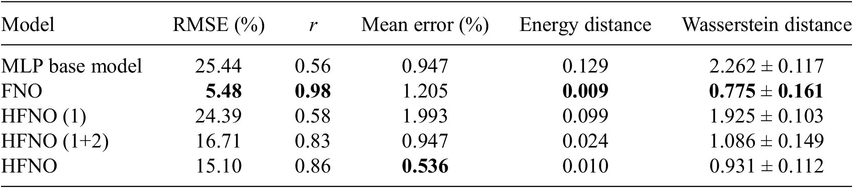
Table 4. Long description
The table consists of six columns and six rows.
Columns from left to right:
1. Model
2. R M S E (percent)
3. r
4. Mean error (percent)
5. Energy distance
6. Wasserstein distance
Data rows:
- M L P base model: R M S E 25.44, r 0.56, Mean error 0.947, Energy distance 0.129, Wasserstein distance 2.262 plus or minus 0.117.
- F N O: R M S E 5.48, r 0.98, Mean error 1.205, Energy distance 0.009, Wasserstein distance 0.775 plus or minus 0.161. (Note: F N O shows the best performance in R M S E, r, Energy distance, and Wasserstein distance).
- H F N O (1): R M S E 24.39, r 0.58, Mean error 1.993, Energy distance 0.099, Wasserstein distance 1.925 plus or minus 0.103.
- H F N O (1 plus 2): R M S E 16.71, r 0.83, Mean error 0.947, Energy distance 0.024, Wasserstein distance 1.086 plus or minus 0.149.
- H F N O: R M S E 15.10, r 0.86, Mean error 0.536, Energy distance 0.010, Wasserstein distance 0.931 plus or minus 0.112. (Note: H F N O shows the lowest Mean error).
The first two metrics assess the model performance in terms of pointwise prediction accuracy, which corresponds to what the models are directly trained for. The relative root mean square error (RMSE) is defined as

and the correlation coefficient r is given by

where
$ \left\langle \cdot \right\rangle $
 denotes the spatial mean over the domain.
The remaining three metrics quantify differences in the distributions of points in the
$ {u}^{+}\left({y}^{+}\right) $
 diagrams shown in Figure 13. For each model, we obtain a distribution in
$ {\unicode{x211D}}^2 $
 that we compare with the ground truth. The mean error corresponds to the RMSE between the mean profiles; the energy distance (Rizzo and Székely, Reference Rizzo and Székely2016) measures the discrepancy between two probability distributions
$ \mu $
 and
$ \nu $
 , and is defined as

where
$ X $
 and
$ {X}^{\prime } $
 are i.i.d. random variables following
$ \mu $
 , and
$ Y $
 and
$ {Y}^{\prime } $
 are i.i.d. random variables following
$ \nu $
 . Finally, the Wasserstein distance (Villani, Reference Villani, Berger, Eckmann, De La Harpe, Hirzebruch, Hitchin, Hörmander, Kupiainen, Lebeau, Ratner, Serre, Sinai, Sloane, Vershik and Waldschmidt2009; Peyré and Cuturi, Reference Peyré and Cuturi2020) quantifies the optimal transport cost required to transform one distribution into the other.
These results indicate that, although the FNO remains the most accurate model in terms of pointwise prediction, the HFNO achieves statistically comparable performance. On average, the HFNO yields slightly better results than the FNO, which appears to exhibit a higher mean error, while both models perform similarly in terms of distributional metrics. Moreover, these results were obtained with a significantly more compact architecture: the trained FNO contains ~5 million parameters, compared to only 1 million for the HFNO. Interestingly, this number can be further reduced by considering truncated versions of the HFNO (HFNO(1) and HFNO(1+2) in Table 4), which remain competitive and satisfactory depending on the desired level of accuracy.
5. Conclusion
In this work, we have presented a Hierarchical Fourier Neural Operator (HFNO) architecture tailored to dynamical systems with multiscale spatial structures. By decomposing the Fourier modes into separate layers corresponding to physically meaningful ranges—energy-containing, inertial, and dissipative scales—the model is able to capture the dominant dynamics at each scale. The use of MLPs for each Fourier layer, complemented by a residual predictor that can take on different forms, allows the network to faithfully reconstruct both large-scale coherent structures and small-scale fluctuations.
Applications to the Kuramoto–Sivashinsky equation, the Kolmogorov flow, and wall modeling in a turbulent channel flow demonstrate the effectiveness of the proposed approach: each Fourier layer predominantly contributes to its assigned wavenumber range, leading to accurate predictions and satisfying generalization capabilities. The hierarchical design not only improves interpretability by linking model components to physical scales but also enhances efficiency by reducing the complexity of each subtask.
Overall, these results highlight the potential of HFNOs for modeling complex turbulent flows in a meshless and physics-informed manner. Future work will focus on extending this framework to higher Reynolds numbers and more realistic three-dimensional flows, as well as exploring adaptive strategies for mode separation to further optimize performance across a broader range of dynamical regimes.
Data availability statement
Replication data and code can be found at https://github.com/marcocayuela/HFNO.
Acknowledgments
The authors gratefully acknowledge Ardeshir Hanifi, Ricardo Vinuesa, and Arivazhagan Geetha Balasubramanian from the Division of Fluid Mechanics, KTH Royal Institute of Technology (Sweden), for kindly providing the open-channel dataset used in this study. The authors also acknowledge the use of the generative AI tool ChatGPT (OpenAI, GPT-5.1, accessed in October 2025) to assist with correcting typographical and grammatical errors in the manuscript. All suggestions generated by the tool were reviewed and validated by the authors.
Author contributions
M.C.: Conceptualization, data curation, data visualization, formal analysis, methodology, validation, and writing original draft. V.L.C.: Resources, supervision, validation, and writing—review and editing. P.J.S.: Resources, supervision, validation, and writing—review and editing. T.S.: Conceptualization, formal analysis, methodology, resources, supervision, validation, and writing—review and editing. All authors approved the final submitted draft.
Funding statement
This research was supported by a grant from the Agence Nationale de la Recherche (ANR), under the funding ID: ANR-22-CE94-0001; EDNNForest.
Competing interests
The authors declare none.
Ethical standard
The research meets all ethical guidelines, including adherence to the legal requirements of the study country.
Appendix A. Kuramoto–Sivashinsky
In this case, the spatial domain is defined by
$ L=22 $
 , and the viscosity parameter is set to
$ \nu =0.7 $
 . Each simulation produces a trajectory consisting of
$ {N}_t $
 = 2000 temporal snapshots on a spatial grid with
$ {n}_x $
 = 1024 points. The simulation time is
$ T=150 $
 and
$ dt=0.075 $
 . For training, we discard the first 150 points that correspond to the transient phase.
In order to select an appropriate number of parallel layers, we trained several HFNO models with different layer configurations. The total number of modes was kept fixed, and the architectures were designed with 1, 2, 4, 8, and 16 layers, yielding the following configurations: [16], [8,16], [4,8,12,16]. … Figure A1 reports the relative RMSE on the test data for each of these models. We select the model corresponding to the knee of the curve, as it provides a good trade-off between overall reconstruction error and effective mode separation.
Relative MSE depending on the number of layers. The red dot indicates the number of layers used in the selected architecture.

A.1. Hyperparameters of the HFNO and FNO models
Tables A1 and A2 report the hyperparameterizations of the FNO used as baseline and the final selected HFNO trained for the KS equation case.
FNO
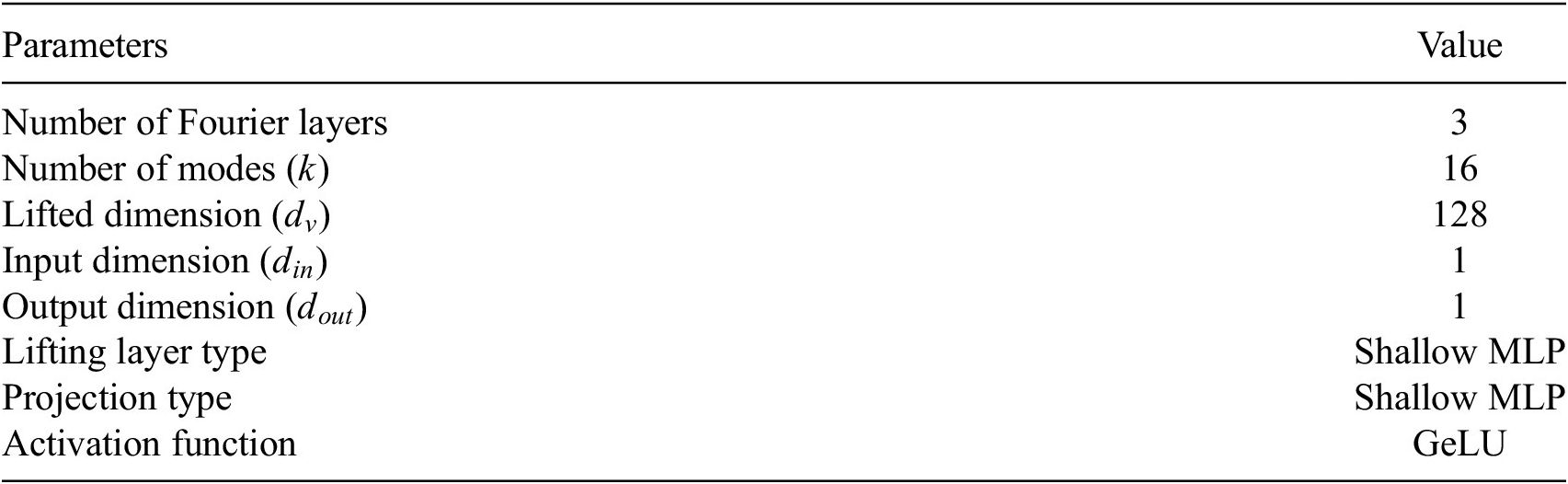
Table A1. Long description
The table consists of two columns titled Parameters and Value.
* Number of Fourier layers: 3.
* Number of modes k: 16.
* Lifted dimension d sub v: 128.
* Input dimension d sub in: 1.
* Output dimension d sub out: 1.
* Lifting layer type: Shallow M L P.
* Projection type: Shallow M L P.
* Activation function: GeLU.
HFNO

Table A2. Long description
The table consists of two columns: Parameters and Value.
* Number of parallel layers: 2.
* Repartition of modes (k): 1 to 6 and 7 to 16.
* Lifted dimension (d sub model): 32.
* Input dimension (d sub in): 1.
* Output dimension (d sub out): 1.
* Lifting layer type: Shallow M L P.
* M L P characteristics: layers: 2; width: 32.
* Activation function: Ge L U.
Appendix B. Kolmogorov flow
In this case, the spatial domain is defined as a square
$ \left[0,2\pi \right]\times \left[0,2\pi \right] $
 . The Reynolds number is set to
$ \mathit{\operatorname{Re}}=90 $
 , and the forcing frequency is
$ {n}_f=4 $
 . The dynamical system is solved using a pseudospectral solver based on a Fourier–Galerkin approach (Canuto et al., Reference Canuto, Hussaini, Quarteroni and Zang1988; Magri, Reference Magri2021; Kelshaw and Magri, Reference Kelshaw and Magri2024). The computational grid is a Cartesian grid of size
$ {n}_x\times {n}_y $
 , with
$ {n}_x={n}_y=128 $
 . Each simulation is initialized with a random velocity field, followed by an initial transient period of 180 time units, after which the subsequent 120 time units are recorded. The simulation time step is set to
$ \Delta t=0.001 $
 , and the number of retained Fourier modes is
$ {n}_k=32 $
 . The resulting trajectories are then preprocessed. They are downsampled in the physical space by a factor of 2 in both spatial directions, and in time by a factor of 60, yielding an effective time step of
$ \Delta t=0.06 $
 for the data used by the models.
B.1. Hyperparameters and architecture of the HFNO and FNO models
In this section, we summarize the architectures used for our experiments. All HFNO models share the same base structure consisting of multiple Fourier layers that are responsible for capturing specific spectral modes. The HFNO variants differ only in the type of residual predictor employed: Linear, CNN, or ESN. The FNO model is composed of stacked Fourier layers without any residual predictor. Tables B1 and B2 below provide a concise description of each component and its parameters.
FNO: classical Fourier Neural Operator architecture
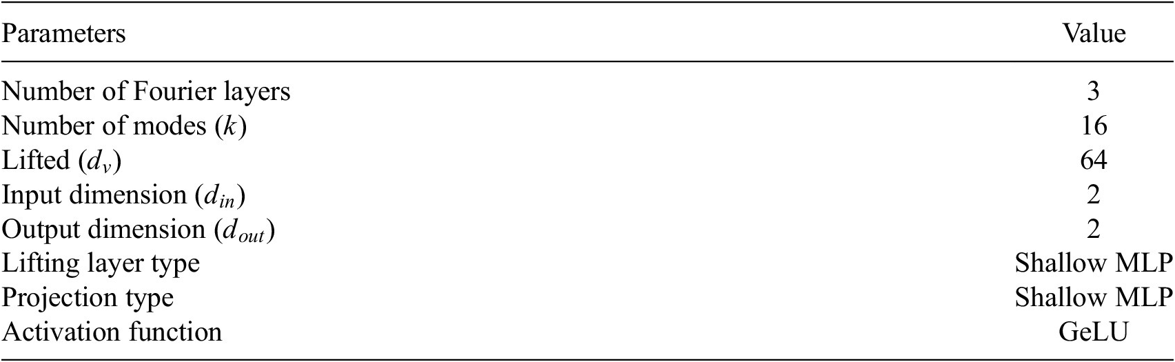
Table B1. Long description
The table consists of two columns: Parameters and Value.
* Number of Fourier layers: 3.
* Number of modes (k): 16.
* Lifted (d sub v): 64.
* Input dimension (d sub in): 2.
* Output dimension (d sub out): 2.
* Lifting layer type: Shallow M L P.
* Projection type: Shallow M L P.
* Activation function: GeLU.
HFNO: base architecture shared by all residual predictor variants

Table B2. Long description
The table consists of two columns: Parameters and Value.
* Number of parallel Fourier layers: 2.
* Repartition of modes (k): 1 to 3 and 4 to 5.
* Separation norm: L sub infinity.
* Lifted dimension (d sub model): 8.
* Input dimension (d sub in): 2.
* Output dimension (d sub out): 2.
* Lifting layer type: Shallow M L P.
* M L P characteristics: layers: 1; width: 128.
* Activation function: GeLU.
B.2. Residual predictors of the Kolmogorov flow
The HFNO variants use different residual predictors. Below are the parameters of each residual predictor.
-
• Linear residual predictor: A simple linear mapping applied to the HFNO output. Key parameters:
-
– Input dimension: $ {d}_{\nu } $
(the lifted dimension) -
– Output dimension: $ {d}_{out} $
(matches HFNO output) -
– Training: end-to-end with HFNO base
-
-
• CNN residual predictor: A shallow convolutional network applied to the HFNO output.
-
– 5 convolutional layers, all with kernel size 3 and padding “same”
-
– Channels per layer: [input → 32 → 64 → 32 → 8 → output]
-
– Activation: default PyTorch (or specify if applied)
-
– Input/Output: matches HFNO output dimensions
-
– Training: end-to-end with HFNO base
-
-
• ESN residual predictor: An Echo State Network applied to the HFNO output to capture temporal dependencies in the residuals. Key parameters:
-
– Reservoir size: 10 k
-
– Spectral radius: 0.9
-
– Input dimension: 2054 (size of the mask used to cut modes × input dimension × 2)
-
– Output dimension: 2054
-
– Training: a posteriori, after the HFNO base has been trained
-


Appendix C. Channel flow
Figure C1 shows the ranges used to select the wavenumber of each Fourier layer. The first line corresponds to the cutoff of the first layer and the second to the second Fourier layer.
Energy spectrum of the channel flow data. The colored dashed vertical lines indicate, from left to right, the 80% and 95%.

Figure C1. Long description
The line graph uses logarithmic scales for both axes. The horizontal x-axis is labeled k sub z and ranges from 10 super 0 to 10 super 2. The vertical y-axis is labeled E (k sub z) and ranges from 10 super -3 to 10 super 1.
* Data Curve: A thick black line begins at the top left at approximately (1, 15) and follows a downward asymptotic curve. The slope becomes steeper as k sub z increases, reaching a value near 10 super -3 at k sub z equals 100. There is a small upward tick at the very end of the curve near k sub z equals 100.
* Vertical Markers: Two dashed vertical lines intersect the curve.
- An orange dashed line is positioned at approximately k sub z equals 8.
- A red dashed line is positioned further to the right at approximately k sub z equals 15.
* Legend: Located in the bottom-left quadrant, it identifies the orange dashed line as the 1st Fourier layer and the red dashed line as the 2nd Fourier layer.
C.1. Hyperparameters and architecture of the HFNO and FNO models
HFNO architecture details

Table C1. Long description
The table consists of two columns: Parameter and Value.
* Number of parallel Fourier layers: 2.
* Mode allocation: 1 to 8 and 9 to 14.
* Separation norm: Directional Mode Partitioning along z axis.
* Lifted dimension (d sub model): 8.
* Input dimension (d sub in): 2.
* Output dimension (d sub out): 2.
* Lifting layer type: Shallow M L P.
* M L P characteristics: layers: 2; width: 128.
* Activation function: Ge L U.
* Residual predictor: C N N (same as for Kolmogorov part).
FNO architecture details

Table C2. Long description
The table consists of two columns: Parameter and Value.
* Number of fourier layers: 3.
* Number of modes (k sub x times k sub y): 24 times 24.
* Lifted dimension (d sub v): 128.
* Input dimension (d sub in): 2.
* Output dimension (d sub out): 2.
* Lifting layer type: Shallow M L P.
* Projection layer type: Shallow M L P.
* Activation function: GeLU.


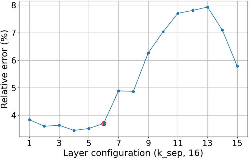

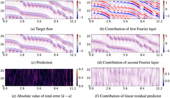


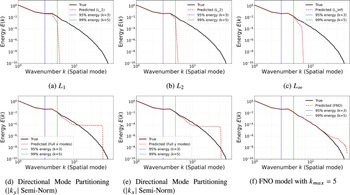





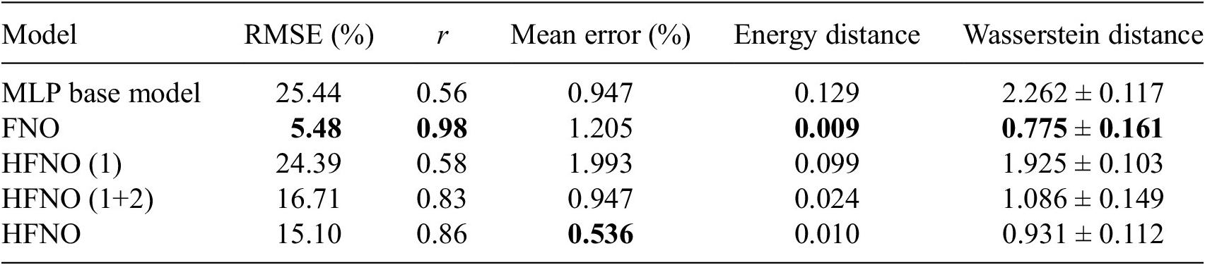
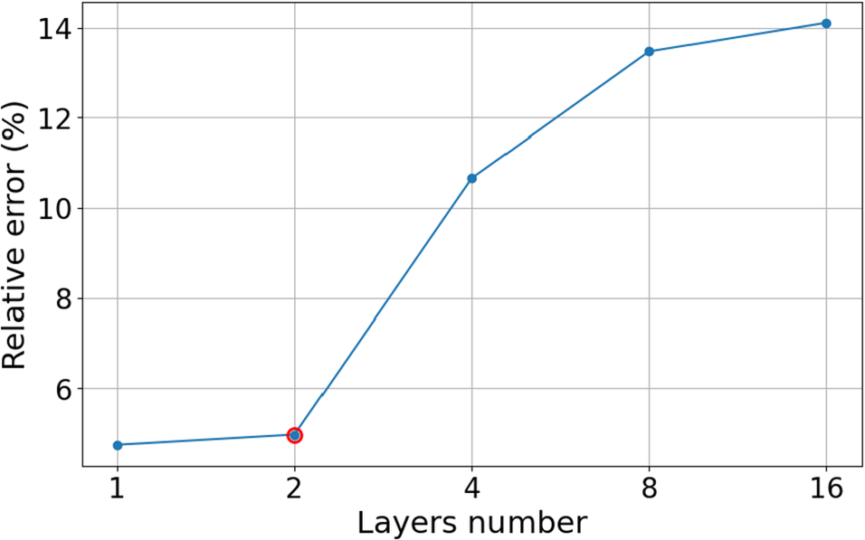
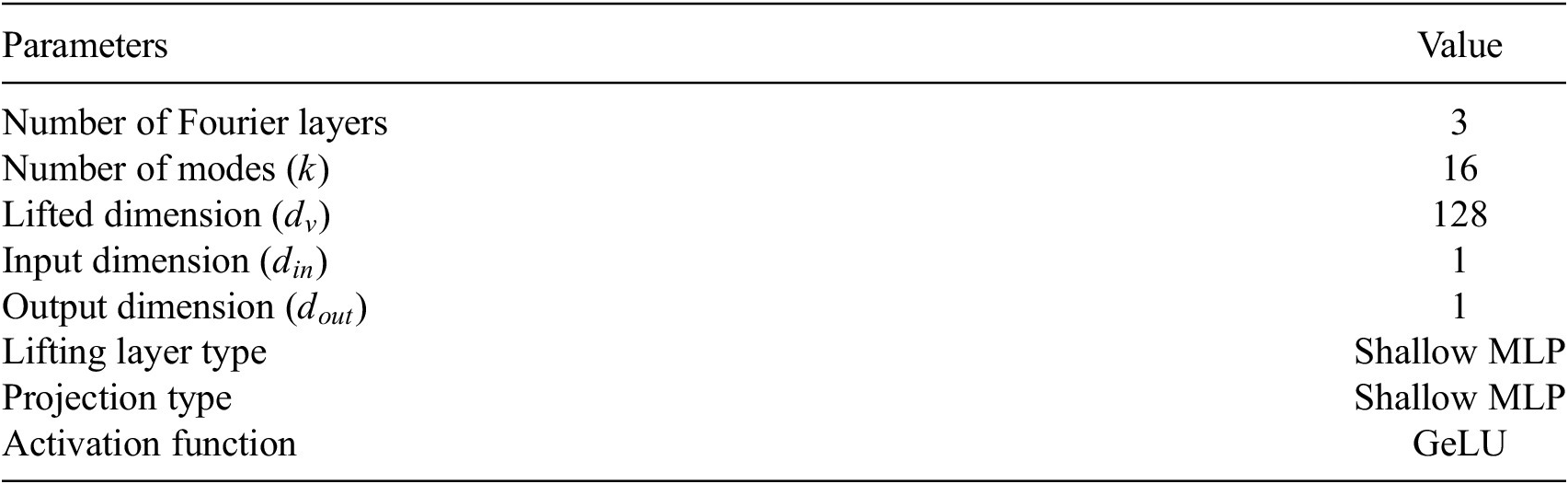
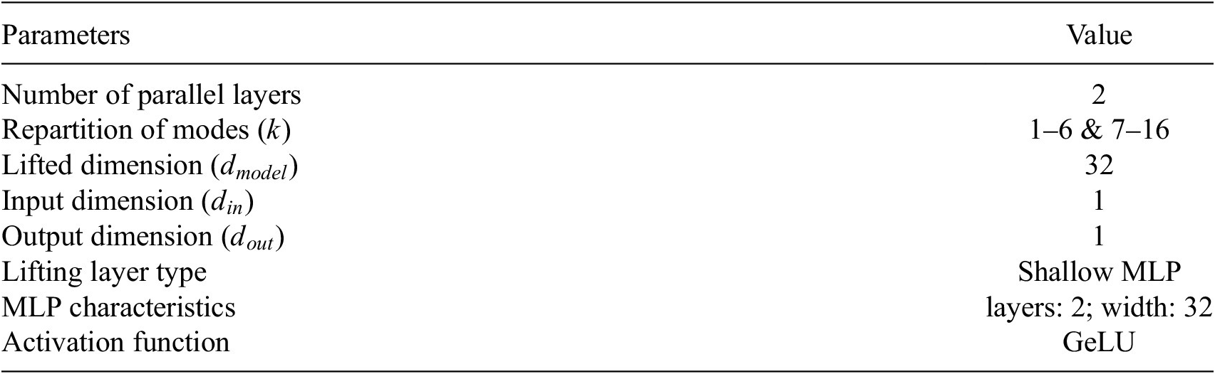
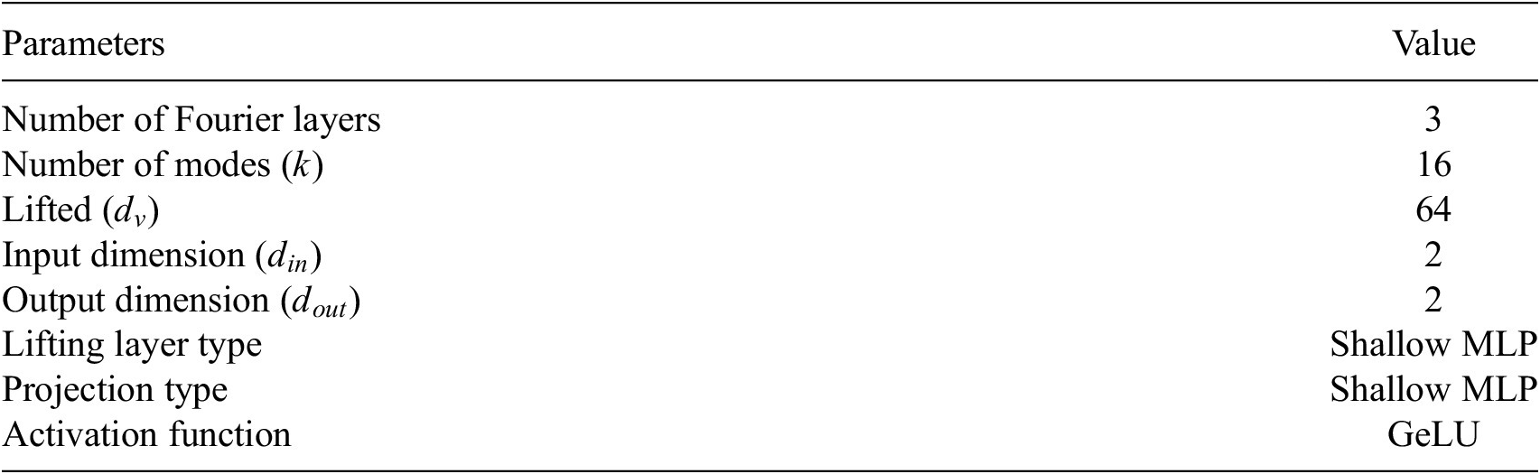
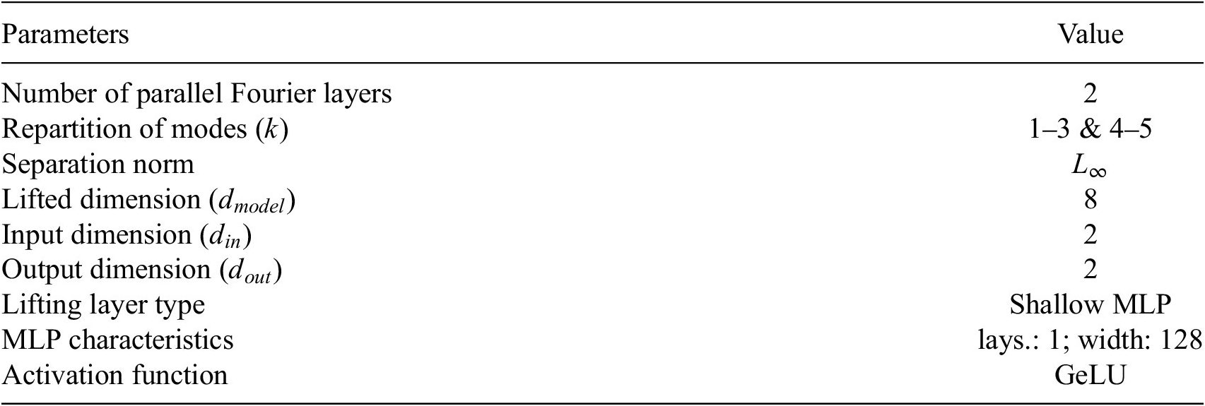

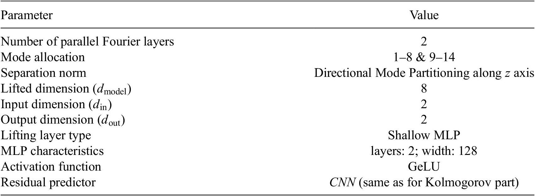
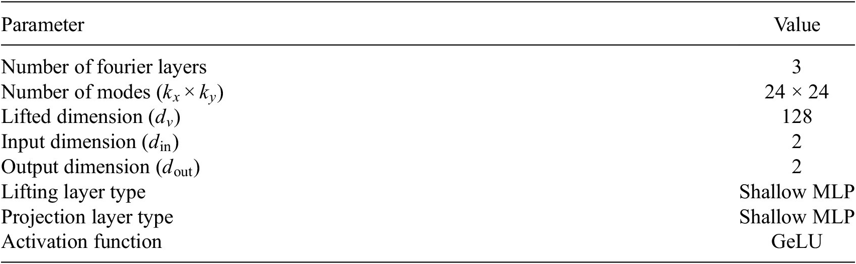

 Open access


Comments
No Comments have been published for this article.