

The holistic-interactionistic view (e.g., Bergman & Magnusson, Reference Bergman and Magnusson1997; Magnusson, Reference Magnusson2001) on individual functioning has influenced several developmental theories that study adaption and maladaption in individuals (Cairns, Reference Cairns1979; Cairns, Elder, & Costello, Reference Cairns, Elder and Costello1996; Cicchetti & Schneider-Rosen, Reference Cicchetti, Schneider-Rosen, Rutter, Izard and Read1986; Ford & Lerner, Reference Ford and Lerner1992; Kagan, Reference Kagan1994; Magnusson, Reference Magnusson1985; Magnusson, Stattin, Damon, & Lerner, Reference Magnusson, Stattin, Damon and Lerner1998; Magnusson & Allen, Reference Magnusson, Allen, Magnusson and Allen1983). This view implies that when studying interrelated factors of individual behavior only in isolation (i.e., ignoring their potentially complex interactions), the factors may lose their meaning and consequence for individual behavior. Developmental psychopathology researchers have greatly benefited from incorporating person-oriented and ideographic approaches in their (variable-orientation dominated) methodological toolbox (Daukantaitė, Lundh, & Wångby-Lundh, Reference Daukantaitė, Lundh and Wångby-Lundh2019; Greenberg, Speltz, Deklyen, & Jones, Reference Greenberg, Speltz, Deklyen and Jones2001; Keller, Spieker, & Gilchrist, Reference Keller, Spieker and Gilchrist2005; Molenaar, Reference Molenaar2010; Mun, Bates, & Vaschillo, Reference Mun, Bates and Vaschillo2010; Sterba & Bauer, Reference Sterba and Bauer2010; von Eye, Reference von Eye2010; von Eye & Bergman, Reference von Eye and Bergman2003). The person-oriented approach (Bergman & Magnusson, Reference Bergman and Magnusson1997) emphasizes the individual as an integrated psychological, biological, and social organism and focuses on individual characteristics of persons, their dynamic development over time, and their variation across contexts. This view has methodological implications which have been discussed by, for example, Bergman (Reference Bergman2001), Bergman, Magnusson, and El Khouri (Reference Bergman, Magnusson and El Khouri2003), and Molenaar and Campbell (Reference Molenaar and Campbell2009), as it requires moving from a variable-oriented “aggregate, then analyze” to a person-oriented “analyze, then aggregate” perspective (cf., Rose, Reference Rose2015). Over the course, various statistical methods have been identified as being ideally suited to evaluate person-oriented research questions (see, e.g., Bergman & Magnusson, Reference Bergman and Magnusson1997; Sterba & Bauer, Reference Sterba and Bauer2010; von Eye, Bergman, & Hsieh, Reference von Eye, Bergman, Hsieh, Overton and Molenaar2015; for a discussion of recent advances in person-oriented statistical methods see Wiedermann, Bergman, & von Eye, Reference Wiedermann, Bergman and von Eye2016).
One of the characteristic features of the person-oriented approach is that research questions are asked in person terms and operationalized as well as analyzed in terms of patterns of events or values of variables (Magnusson & Stattin, Reference Magnusson, Stattin, Damon and Lerner1998). In the domain of categorical variables, configural frequency analysis (CFA; Lienert, Reference Lienert1968; von Eye, Reference von Eye1990) is therefore a prime method for evaluating hypotheses that are compatible with the person-oriented approach (von Eye, Reference von Eye2010). CFA has been successfully applied in a number of fields. We present two examples.
In a study on violent offenders, Hildebrand Karlén, Nilsson, Wallinius, Billstedt, and Hofvander (Reference Hildebrand Karlén, Nilsson, Wallinius, Billstedt and Hofvander2020) used exploratory CFA, in combination with variable-oriented analyses, to identify potential configurations of early-onset externalizing problems in adolescence that are predictive of problem aggregation patterns in early adulthood in criminal behavior, substance abuse, and psychiatric comorbidity. Two types resulted. The first describes patterns of physical assault, threats and robbery with later sexual delinquency and arson. The second describes patterns of physical assault, threats, and robbery, which are later followed by murder, sexual delinquency, and arson. This result supports Stattin and Magnusson's (Reference Stattin and Magnusson1996) theory according to which patterns of externalizing problems tend to gravitate to clusters of behavior problems, and that concentration of several problem areas is prognostic for adjustment problems in adulthood.
The second example, which leads us directly to the topic of this article, can be found in psychophysiological research (Müller, Netter, & von Eye, Reference Müller, Netter and von Eye1997). The authors performed a two-group CFA in which they examined bivariate catecholamine response curves in normo- and hypertensive patients under stress. Results suggested in the form of types and antitypes that hypertensives respond to stress with decreases in their high tonic adrenaline values. In a two-group comparison, the authors found that hypertensives and normotensives also differ in that maladaptive patterns of response to stress are more frequent in hypertensives than in normotensives – a statement that cannot be justified by standard CFA; configural group comparison is required.
Configural frequency modeling has been extended in a number of ways, including CFA for longitudinal data (von Eye, Mun, & Bogat, Reference von Eye, Mun and Bogat2008) and mediational processes (von Eye, Mun, & Mair, Reference von Eye, Mun and Mair2009). Although both of these models are person-oriented in nature, they still assume that identified extreme patterns (so-called CFA types and antitypes; Lienert, Reference Lienert1968) hold for the entire population under study. The study of subpopulations, for example, through the inclusion of moderator variables, constitutes a continuing methodological challenge in configural frequency modeling. In the presence of variability of effects – that is, in the presence of moderation – models of CFA have been developed by von Eye, Mair, and Mun (Reference von Eye, Mair and Mun2010). In addition, decision tree techniques have been incorporated in configural frequency modeling by Lautsch and Ninke (Reference Lautsch and Ninke2000) as well as Melcher, Lautsch, and Schmutz (Reference Melcher, Lautsch and Schmutz2012). These authors suggested to combine chi-squared automatic interaction detectors (CHAID; Kass, Reference Kass1980) with prediction CFA (P-CFA; Lienert & Krauth, Reference Lienert, Krauth and Eckensberger1973). In their approach, CHAID is used to detect heterogenous configurations with respect to the occurrence of an event of interest (the outcome variable), that is, a binary outcome variable is partitioned into several subgroups and covariates (partitioning variables) are used to characterize the subgroups. In a second step, P-CFA is then used to validate potential extreme cells as CFA types or antitypes (to be defined in detail below). More recently, von Eye, Wiedermann, and von Weber (Reference von Eye, Wiedermann and von Weber2019) proposed configural and log-linear models for the analysis of decision tree structures. In essence, the authors make use of special contrasts corresponding to the decision made in a tree, and the so-called Schuster transformation (von Eye, Schuster, & Rogers, Reference von Eye, Schuster and Rogers1998; Wiedermann & von Eye, Reference Wiedermann and von Eye2020b) is used to guarantee that specified contrasts can be interpreted as intended. In a second step, CFA is used to identify extreme patterns that represent the sequence of decisions. For an application see Stemmler, Heine, and Wallner (Reference Stemmler, Heine and Wallner2019).
The present study continues the development of methods for the analysis of moderation effects in configural frequency modeling by making use of model-based recursive partitioning (MOB; Zeileis, Hothorn, & Hornik, Reference Zeileis, Hothorn and Hornik2008). Based on recursively partitioned generalized linear models (GLMs) (Rusch & Zeileis, Reference Rusch and Zeileis2013), we present the specification of CFA trees. The proposed approach differs from the previous attempts to combine tree-based methods and CFA. Instead of using tree methods to determine configurations of interest, we use MOB to recursively partition the CFA model itself. The MOB CFA algorithm results in a regression tree. Each terminal node of the tree is defined by a separate CFA model with potentially varying type/antitype patterns. While the MOB CFA algorithm can be applied to a large family of CFA models (the method can be applied as long as the base model can be written as a log-linear model), in the present article, we present applications for first-order CFA (Lienert, Reference Lienert1968) and P-CFA (Lienert & Krauth, Reference Lienert, Krauth and Eckensberger1973) in the presence of complex moderation. The moderation process is described in the form of a tree leading to subgroups for which unique CFA pattern results are possible. Subgroup-specific CFA type/antitype patterns open the door to identify population types/antitypes (i.e., type/antitype patterns that hold for the entire set of data) and subpopulation types/antitypes (i.e., patterns that are specific to certain subgroups in the population). We use two empirical data examples from the field of school mental health research for illustrative purposes. In the first example, first-order MOB CFA is applied to detect (sub)population types/antitypes in student problem behavior patterns. In the second example, we apply MOB P-CFA in the context of evaluating the intervention effect of a teacher classroom management program on students’ internalization problems. To demonstrate the statistical performance of the method, we present the results from two Monte Carlo simulation studies suggesting that CFA trees can be detected with sufficient statistical power in particular in the context of large samples and large variability of effects.
The article is structured as follows: First, we introduce CFA and discuss the steps taken when analyzing a cross-classification table with respect to the occurrence of configurations. Second, we provide a nontechnical introduction into recursive partitioning (MOB). Third, we discuss MOB in the context of a Poisson GLM (McCullagh & Nelder, Reference McCullagh and Nelder1989) to estimate a first-order CFA, present results of a simulation study, and illustrate the method using data from school mental health. Fourth, we present CFA tree models for P-CFA, present simulation results, and give an empirical example. Fifth, we discuss sensitivity analysis methods to evaluate the stability of CFA model trees and demonstrate their application using the two data examples. Finally, the article closes with a discussion on the implications of the findings for school mental health, potential extensions, and potential limitations of the presented approach.
An Overview of Configural Frequency Analysis
CFA (Lienert, Reference Lienert1968; von Eye, Reference von Eye1990; von Eye et al., Reference von Eye, Mair and Mun2010; von Eye & Gutiérrez Peña, Reference von Eye and Gutiérrez Peña2004) is a widely applied method to analyze configurations of categorical variables. Here, configurations are characterized as ensembles of categories that define the cells of cross-classification tables (Lienert, Reference Lienert1968). In configural frequency modeling one asks whether the number of times the configurations occur in the data can be expected under a specific model, the so-called base model (von Eye, Reference von Eye2004). The orientation of deviations from expectancy classifies the deviating cell as either a CFA type (i.e., the configuration occurs more often than expected under the base model) or a CFA antitype (i.e., the configuration occurs less often than expected under the base model). Conducting CFA consists of four steps: (a) specification of a CFA base model, (b) selection of a significance procedure for type/antitype detection, (c) performing CFA under protection of the nominal significance level (protection is needed because of multiple testing), and (d) interpretation of the types/antitypes. In the following paragraphs, we give a summary of each of the steps.
Step 1: Specification of CFA base model
The CFA base model is a theory-driven probability model used to estimate expected frequencies of the configurations. Here, it is important to note that the base model contains all effects that are not of interest. If this model is rejected, the effects of interest (i.e., the effects that are not part of the base model) are needed to explain the data. Therefore, CFA identifies sectors in the data space where effects are particularly noticeable. Such data regions are expressed in terms of CFA types and antitypes. The majority of CFA base models can be written as log-linear models log(E[m]) = X λ with E[m] being the expected frequencies, X is the design matrix, and λ is the vector of model parameters (for an exception see, for example, symmetry models discussed in von Eye, Reference von Eye2002). Base models can be global (e.g., first-order CFA), regional (e.g., k-group CFA), they can incorporate special effects (e.g., CFA with covariates), and they can come in the form of multistep models (e.g., mediation CFA; for a classification of CFA base model see von Eye & Wiedermann, Reference von Eye and Wiedermann2021). Instead of searching for the most parsimonious model to explain variable associations (a perspective usually taken in log-linear modeling; Christensen, Reference Christensen1997), CFA identifies configurations that contradict the base model the strongest. Three characteristics are of central importance when formulating CFA base models: (a) interpretability, (b) parsimony, and (c) the sampling scheme. Interpretability refers to the fact that every base model must be specified in a way that there exists only one reason why CFA types and antitypes can occur; this reason is the effect of interest that is not part of the CFA base model. Parsimony implies that the number of parameters of the base model must be as small as possible while, at the same time, as complete as needed to guarantee that the emerging types/antitypes can be interpreted as intended. Finally, decisions concerning base models need to take into account the sampling scheme of the study (von Eye & Schuster, Reference von Eye and Schuster1998). Here, one distinguishes between Poisson, multinomial, and product-multinomial sampling. Under Poisson sampling, neither the sample size nor the frequencies are determined a priori by the researcher. In the case of multinomial sampling, the sample size is fixed a priori, and under product-multinomial sampling, the number of observations in variable categories are determined a priori. The sampling scheme has implications for the selection of base models and significance tests discussed in the next section.
Before we move on with the second step of configural frequency modeling, selection of significance tests, we want to emphasize one important feature of log-linear model specification in the context of recursive partitioning. Application of MOB requires that the log-linear model of interest is specified on the individual level. That is, instead of regressing aggregated cell counts on the design matrix, one regresses a vector m i (with i = 1, …, n indexing the participants), with m i = 1 if the configuration is observed for subject i and m i = 0 otherwise (also called the expanded-data method; Hunt, Friesen, Sama, Ryan, & Milton, Reference Hunt, Friesen, Sama, Ryan and Milton2015). The reason for this is that often continuous splitting variables (e.g., age) are included in addition to categorical splitting variables (such as gender). When all splitting variables are categorical, individual level data are no longer required. Here, however, we treat the more general individual-level case. An individual-level log-linear model can be written as

with i = 1, …, n referring the ith subject; ${\bf X}_i$ represents the subject-level design matrix consisting of 2J × n rows (with J being the number of binary variables and n representing the sample size), and λ being the subject-level vector of parameters. Case-wise and standard aggregated log-linear models give similar parameter and standard error estimates (except for the intercept parameter which depends on the sample size; Christensen, Reference Christensen1997). Example specifications of (case-wise) subject-level design matrices are given below. Case-wise definitions of design matrices have been used, for example, in the context of modeling continuous subject-specific effects of choice behavior in the context of log-linear Bradley Terry models (Hatzinger & Dittrich, Reference Hatzinger and Dittrich2012) and in modeling covariate effects on inter-rater agreement (Hunt et al., Reference Hunt, Friesen, Sama, Ryan and Milton2015). In the present context, we make use of the expanded-data method to describe CFA base models on the level of the individual.
Step 2: Selection of significance tests
Significance tests in CFA evaluate the CFA null hypothesis $H_0\colon m_k = \hat{m}_k$ where m k are the observed cell frequencies and $\hat{m}_k = E[ {m_k} ]$
 denote the expected cell frequencies (k indexes the configurations and E indicates expectancy) estimated under some CFA base model. CFA types emerge when $m_k \gt \hat{m}_k$
 and CFA antitypes emerge when $m_k \lt \hat{m}_k$
 . If the null hypothesis is retained, configuration k is neither a type nor an antitype. In the present study, we focus on the binomial test as one of the first tests that have been suggested in the context of CFA (Lienert & Krauth, Reference Lienert, Krauth and Eckensberger1973). The test has the advantage that it can be applied under any sampling scheme. Further, the test is nonparametric and exact (thus, there is no need to assume that a test statistic is sufficiently close to the sampling distribution). The binomial test, however, comes with lower power compared to some alternatives such as the local Pearson χ2 test or von Eye and Mair's (Reference von Eye and Mair2008) procedure based on standardized Pearson residuals. The power disadvantage of the binomial test disappears for large sample scenarios (von Eye & Wiedermann, Reference von Eye and Wiedermann2021) which are arguably preferable when searching for population subgroups that differ qualitatively from each other.
Step 3: Performing CFA under alpha protection
To determine whether a cell significantly differs from expectation, one needs to select a nominal significance level α. Because significance tests are repeatedly performed under the same null hypothesis, α protection methods are required to avoid inflated Type I error rates (i.e., inflated rates of false positive results). The issue is further exacerbated by the fact that, in CFA, significance tests depend on each other. For example, von Weber, Lautsch, and von Eye (Reference von Weber, Lautsch and von Eye2003) demonstrated that, when analyzing a simple 2 × 2 cross-classification with a first-order CFA, the four significance tests are completely dependent upon one another.
Several approaches are available for α adjustment. Bonferroni α correction, that is, using a nominal significance level of α* = α/k with k indicating the number of significance tests performed, is widely accepted for this endeavor. However, several alternative α adjustment techniques (see, e.g., Dunnett & Tamhane, Reference Dunnett and Tamhane1992; Hochberg, Reference Hochberg1988; Holland & Copenhaver, Reference Holland and Copenhaver1987; Olejnik, Li, Supattathum, & Huberty, Reference Olejnik, Li, Supattathum and Huberty1997) can be used which are known to be more powerful than Bonferroni adjustment. In the following applications of CFA, we make use of the more conservative Bonferroni procedure with the understanding that the performance of MOB CFA can potentially be improved by selecting more liberal α adjustment techniques.
Step 4: Interpretation of CFA types/antitypes
Following von Eye et al. (Reference von Eye, Mair and Mun2010), the interpretation of CFA types/antitypes is based on four sources of information. The first of these is the meaning of the variable categories that define a configuration. The second source are the implications of the applied base model. For example, when the base model only includes the main effects of the variables that span the cross-classification (a so-called first-order CFA), CFA types/antitypes show where in the data space variable interactions are located (or most visible). When the base model excludes the relations between predictor and outcome variables, CFA types/antitypes indicate the predictor configurations that are particularly strongly related to specific configurations of the outcome variable(s). The third source of information is the sampling scheme (e.g., Poisson, multinomial, product-multinomial). The sampling scheme places constraints on the specification of a base model which have implications for the hypotheses that can be tested in the base model. The fourth source is information that is carried by variables that are not part of those that span the cross-classification under study (e.g., explicitly distinguishing between classification indicators used to separate independent variables). This information can be used, for instance, by including variables as covariates or moderator variables. Covariates have the potential that CFA types/ antitypes emerge or disappear. Moderators can identify type/antitype patterns that differ across groups. In the present approach, these separate independent variables come in the form of splitting variables used to partition the data. In the following section, we introduce principles of recursive partitioning in the context of log-linear CFA base models.
Model-based Recursive Partitioning
Tree-based methods, valuable alternatives to standard parametric methods, have extensively been discussed in the past (see, e.g., Breiman, Friedman, Olshen, & Stone, Reference Breiman, Friedman, Olshen and Stone1984; Hothorn, Hornik, & Zeileis, Reference Hothorn, Hornik and Zeileis2006; Quinlan, Reference Quinlan1993; Morgan & Sonquist, Reference Morgan and Sonquist1963; Strobl, Malley, & Tutz, Reference Strobl, Malley and Tutz2009; Zhang & Singer, Reference Zhang and Singer2010). In conventional classification and regression tree (CART) and CHAID algorithms, it is the aim to recursively partition the covariate space to identify subgroups with different values of an outcome variable. In contrast, MOB (Zeileis et al., Reference Zeileis, Hothorn and Hornik2008) uses parameters of a predefined parametric model as the basis for recursive partitioning. The MOB algorithm partitions a set of predefined covariates (so-called splitting variables) by evaluating parameter instabilities of a parametric model. More specifically, a parametric model is formulated to represent an empirical question of interest. In the present study, the parametric model of interest is a log-linear model that defines the meaning of CFA types/antitypes, should they exist. This log-linear model is then fed into the MOB algorithm to evaluate whether covariates (splitting variables) exist which alter the parameters of the log-linear model. Making use of the GLM framework, we specify the log-linear model as Poisson regression. That is, let Y be the count response of interest with the mean E[Y] = μ (E being the expected value operator) and X defines a matrix collecting independent variables . The mean of Y is modeled using a linear predictor η = Xβ using g(μ) = η with g referring to the link function and β defines the vector of regression coefficients. In the context of log-linear modeling, one often replaces β with the parameter vector λ indicating the effects associated with contrasts in the design matrix X. We can write the log-linear model in the form of a Poisson regression model using a log-link,

Identifying a parameter instability in λ with respect to a partitioning covariate implies that subgroup-specific conditional effects exist in the data. The (score-based) generalized M-fluctuation test (Zeileis & Hornik, Reference Zeileis and Hornik2007) is used to assess the stability of (log-linear) model parameters along selected splitting variables. To protect the global significance level, score tests are used with Bonferroni α correction. The type of M-fluctuation test depends on the measurement level of the splitting variable. For continuous variables, the supLM statistic (Andrews, Reference Andrews1993) is employed; for categorical splitting variables χ2 statistics by Hjort and Koning (Reference Hjort and Koning2002) are applied. A parameter instability is captured by fitting separate models for each subgroup. To split the sample along the selected covariate, the cut-point with the largest model fit improvement is used. The algorithm terminates in end nodes when no parameter instabilities are found or when the size of the subsample is smaller than an a priori selected minimum (Rusch & Zeileis, Reference Rusch and Zeileis2013; Zeileis et al., Reference Zeileis, Hothorn and Hornik2008). To avoid overfitting (in particular, when sample sizes are very large), post-pruning strategies based on information criteria (such as, e.g., the Akaike information criterion; AIC) have been suggested to prune back splits that do not improve model fit (Zeileis et al., Reference Zeileis, Hothorn and Hornik2008). Each end node consists of a local log-linear model

with g indexing the detected subgroups (g = 1, …, G). Subsequently, these G local log-linear models are treated as subgroup-specific CFA base models. Before we move on and present model tree specifications for first-order CFA (as one of the most important CFA models) and P-CFA (in which one distinguishes between predictor and outcome variables), we briefly introduce a graphical visualization of the MOB CFA end nodes.
Mosaic displays as data visualization
Regression trees offer a representation of potentially complex moderation mechanisms in the form of accessible tree structures. In addition, depending on the models displayed in the end nodes, differences in model parameters can be visualized using graphical methods as well. In the context of configural frequency modeling, partitions found via MOB CFA can be represented as n-way contingency tables. Thus, mosaic plots (or mosaic displays; Hartigan & Kleiner, Reference Hartigan and Kleiner1984; Friendly, Reference Friendly1994, Reference Friendly1995; for an example see Figure 5) constitute an attractive graphical method to summarize partition-specific CFA results (for a discussion of the use of mosaic displays in the CFA context see Mun, von Eye, Fitzgerald, & Zucker, Reference Mun, von Eye, Fitzgerald and Zucker2001).
Mosaic plots have become the primary method to visualize frequencies of a n-way contingency tables and to analyze structures of log-linear models (Friendly, Reference Friendly1994, Reference Friendly1995). In mosaic plots, cell frequencies are represented by tiles (rectangles) that are proportional to the cell frequencies of the cross-table. The idea is best introduced using a simple two-way table. The expected frequencies under independence can be displayed as tiles whose widths are proportional to the total frequency in each column (the first variable), and whose heights are proportional to the total frequency in each row (the second variable). Then, the area of the tile is proportional to the cell frequency. Specifically, a unit area is divided into bars with width equal to the marginal frequencies (probabilities) of the first variable, and these bars are divided into tiles with heights being equal to the conditional frequencies (probabilities) of the second variable. The resulting area reflects the total quantity (cell frequencies) in the cross-table of the variables. When two variables are independent, the tiles of the mosaic plot will align (i.e., all tiles in each row have the same height). Not aligning tiles indicate dependency structures between the two variables. Several pattern detection approaches can be imposed on the mosaic plot through making use of coloring and shading of tiles (Friendly, Reference Friendly1994).
In the present context, feasibility of mosaic plots depends on the number of variables involved and the complexity of the base model. Here, the maximum number of variables to meaningfully use mosaic displays simply depends on the readers’ familiarity with interpreting mosaic plots. When the model is too complex to be visualized in an accessible way, simple CFA summary tables can be used instead of mosaic plots. In the first empirical example given below, we use CFA summary tables, in the second example, we give an example using mosaic displays. Although readers may be required to familiarize themselves with decoding statistical information from mosaic displays first, this type of visualization is ideally suited to display MOB CFA differences across partitions. In its simplest form, mosaic plots can be generated for the gth contingency table. In addition, each partition-specific mosaic plot can be shaded according to the status of the configuration as “no deviation” (marked gray in the plots given in Figures 5 and 6), type (marked green), or antitype (marked red), that is, the pattern detection method is the presence/absence of types/antitypes itself. However, more complex representations that take into account fit information of partition-specific log-linear models can be used as well (cf. Friendly, Reference Friendly1994, Reference Friendly1995).
First-order CFA Trees
The first CFA tree model discussed here builds on the first-order CFA base model. This model constitutes the classic version of CFA and was originally proposed by Lienert (Reference Lienert1968). The model only takes main effects of all variables into account and, thus, assumes independence of variables. If CFA types/antitypes exist, they can only emerge due to the presence of interactions (of any order) among variables. For J variables (Xj, j = 1, …, J), the first-order base model can be written as

with λ being the intercept and $\lambda ^{X_j}$ being the main effect parameter for Xj. For J = 3 binary variables (i.e., in case of a 2 × 2 × 2 cross contingency table), the effect coded design matrix X for this model is

The first column of the design matrix represents the intercept, the second column specifies the main effect for the first variable (X 1), and the third and fourth column give the main effects for the second and third variable (X 2 and X 3). Each column contrasts the two categories of each variable (e.g., the presence of a symptom is coded with 1 and the absence of the symptom is indicated by −1).
In CFA trees, we assume that parameters of the base model can vary across subgroups (partitions) of the data. Formally, the first-order MOB CFA model for g = 1, …, G subgroups and j = 1, …, J indicators is given by

with λ g being the subgroup-specific intercept and $\lambda _g^{X_j}$ specifying the subgroup-specific main effects. Varying log-linear model parameters across subgroups open the door to the presence of subgroup-specific CFA types and antitypes. Splitting variables of CFA trees can be conceptualized as moderators. Tree estimation is based on a reformulation of the log-linear model as a Poisson count regression model (often referred to as the “Poisson trick”) making use of the fact that Poisson counts are jointly multinomially distributed (Agresti, Reference Agresti2002). To apply the MOB algorithm, one requires a case-wise design matrix for the Poisson regression model. To give an example, consider the case of two individuals, three binary classification variables (X 1–X 3; 0 = symptom absence, 1 = symptom present), and two continuous splitting variables U and V. For Person 1, suppose we observe X 1 = X 2 = X 3 = 0 (i.e., the configuration {0 0 0}) as well as U = u 1 and V = v 1. In contrast, for Person 2, we obtain the configuration {1 0 0} together with U = u 2 and V = v 2. The corresponding case-wise design matrix for the two participants then takes the form

where m gives the observed frequencies for all possible patterns based on the three X indicators (the intercept is implied). Because {0 0 0} was observed for the first person, we use m = 1 for this particular configuration, and m = 0 for the remaining seven configurations. Similarly, for Person 2, we use m = 1 for {1 0 0} and m = 0 otherwise. For both participants, values of the splitting values U and V (u 1, u 2, v 1, and v 2) are each repeated eight times according to the number of configurations. The resulting design matrix contains 16 rows (eight possible patterns for each of two participants). More generally, for n participants and J binary indicators, the number of rows of the case-wise design matrix is given by n ⋅ 2J. In the corresponding MOB Poisson regression model, m is treated as the response, the dummy variables for X 1–X 3 are used as independent variables (effect coding could be applied as well), and U and V serve as splitting variables. Within MOB, generalized M-fluctuation tests (Zeileis & Hornik, Reference Zeileis and Hornik2007) are used to assess stability of model parameters for the indicators X 1, X 2, and X 3 along the splitting variables U and V. The resulting partitions can be interpreted as terminal nodes of a CFA tree containing separate first-order CFA models with varying parameters and (potentially) partition-specific types and antitypes. In the following section, we illustrate the performance of first-order MOB CFA using Monte Carlo simulations.
Simulation Study I
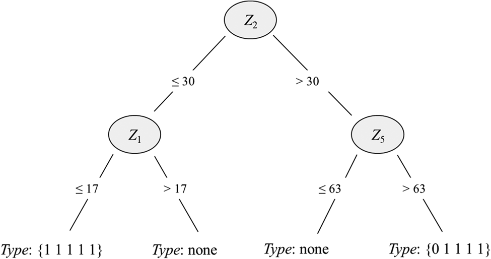
To illustrate the performance of MOB CFA in the context of a first-order base model, a simulation study was performed using the R statistical programing environment (R Core Team, 2020). The data generating mechanism is summarized in Figure 1. Four subgroups based on three relevant partitioning variables, Z 1, Z 2, and Z 5, among a set of ncov covariates were generated. The number of covariates (Z 1, …, Zncov) was either ncov = 5 or 10. Following Dusseldorp and Van Mechelen (Reference Dusseldorp and Van Mechelen2014), Fokkema, Smits, Zeileis, Hothorn, and Kelderman (Reference Fokkema, Smits, Zeileis, Hothorn and Kelderman2018), and van Wie, Li, and Wiedermann (Reference van Wie, Li and Wiedermann2019), all covariates were randomly drawn from a multivariate normal distribution with means for Z 1, Z 2, Z 4, and Z 5 of 10, 30, −40, and 70. The means of the remaining covariates (Z 3 and depending on the value of ncov, Z 6, …, Z 10) were randomly generated from the uniform distribution on the interval [−70, 70]. The standard deviation of all covariates was set to 10 and pairwise correlations of all covariates were fixed at 0.3. Following Schrepp (Reference Schrepp2006), simulated configurations were based on a set of dichotomous indicators, for example, representing the absence or presence of symptoms that occur randomly in the underlying population (0 = symptom absent, 1 = symptom present). In the simulation, the number of indicators was set to 5 and the probabilities of observing the symptoms were randomly drawn from a uniform distribution with a minimum of 0.05 and a maximum of 0.15. To simulate the occurrence of CFA types, in the next step, observed (individual-level) symptom configurations were replaced with predefined type configurations with probabilities δ = 0.20, 0.25, 0.30, and 0.35. The predefined type configurations varied across subgroups. In Subgroup 1 (individuals for which Z 1 ≤ 17 and Z 2 ≤ 30), the configuration {1 1 1 1 1} constitutes a CFA type, in Subgroups 2 (Z 1 > 17 and Z 2 ≤ 30) and 3 (Z 2 > 30 and Z 5 ≤ 63) no types occurs, and in Subgroup 4 (Z 2 > 30 and Z 5 > 63) the configuration {0 1 1 1 1} is a CFA type. In other words, in one subgroup, a CFA type was characterized by the occurrence of all five symptoms, and in a second subgroup, a CFA type is characterized by the absence of the first symptom and the presence of the remaining four symptoms. Sample sizes were set to n = 500, 1,000, and 1,500. The simulation design was fully crossed resulting in 2 (number of covariates) × 3 (sample size) × 4 (effect size δ) = 24 simulation conditions. For each simulation condition, 100 samples were generated.
Data-generating mechanism of simulated first-order configural frequency analysis (CFA) trees based on three splitting variables Z 1, Z 2, and Z 5.

For each generated sample, we computed the subject-specific (effect coded) design matrix of a first-order CFA for the five binary indicators to explain the observed configuration frequencies. MOB was used to identify (potentially) better fitting local first-order CFA models. Bonferroni-corrected parameter stability tests were performed using a nominal significance level of 5%. Regression trees were estimated with a maximal depth of three, limiting the number of terminal nodes to eight. The function GLM tree of the R package partykit (Hothorn & Zeileis, Reference Hothorn and Zeileis2015) was used for MOB estimation. Next, for each subgroup identified through MOB, we performed a separate first-order CFA with Bonferroni-corrected binomial tests (implemented in the R package confreq, Stemmler & Heine, Reference Stemmler and Heine2017) to evaluate the presence of types and antitypes.
Results
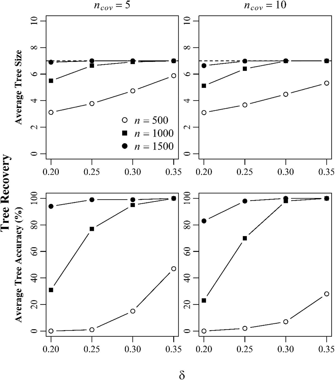
Figure 2 summarizes the performance of the MOB CFA algorithm to identify the correct tree structure. We focus on the size and the overall accuracy of the estimated trees. Following Fokkema et al. (Reference Fokkema, Smits, Zeileis, Hothorn and Kelderman2018) and van Wie et al. (Reference van Wie, Li and Wiedermann2019), we defined an accurately recovered tree as one that (a) consists of seven nodes in total (three splitting and four terminal nodes), (b) uses Z 2 as the first splitting variable with a value of 30 ± 5 (i.e., ± half the population standard deviations of the partitioning covariates), (c) identifies Z 1 as the next split on the left with 17 ± 5, and (d) uses Z 5 as the final splitting variable on the right side of the tree with a value of 63 ± 5.
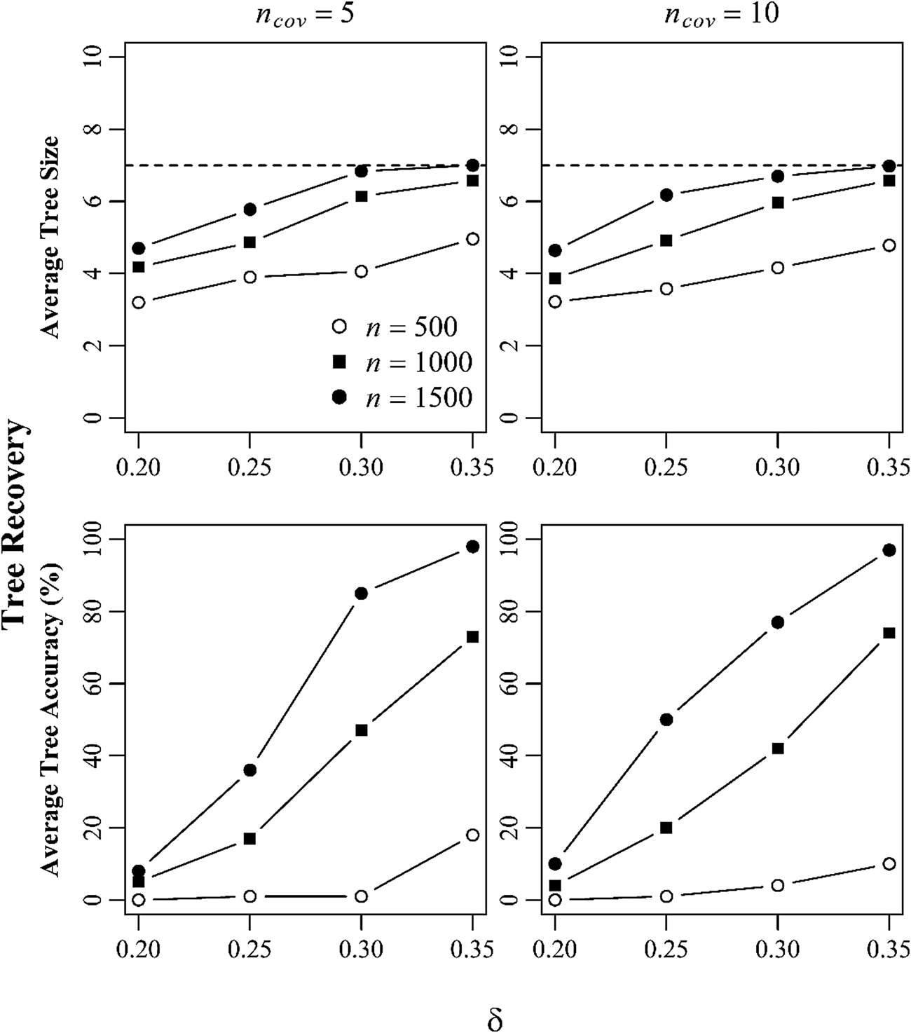
Average tree size and accuracy of recursively partitioned first-order configural frequency analysis (CFA) as a function of sample size (n), number of covariates (ncov), and probability of CFA types (δ).

The upper panel of Figure 2 gives the average tree size as a function of the number of covariates, sample size, and the probability to observe a subgroup-specific CFA type (δ). For large sample sizes (n = 1,500), the average tree size is close to the true one, independent of the number of covariates and the level of δ. For smaller sample sizes, the average tree size tends to be smaller, in particular, when the probability of CFA types is small as well. For example, for n = 1,000 and δ = 0.20, we obtain an average tree size of 6.77 (SD = 0.70). For n = 500 and δ = 0.20, the average tree size declines to 3.11 nodes on average (SD = 1.10). Similarly, a large number of covariates also slightly decreases the average tree size. This effect is, however, mitigated for larger samples. For n = 500, 1,000, and 1,500, we observe an average tree sizes of 4.38 (SD = 1.57), 6.52 (SD = 0.98), and 6.98 (SD = 0.22) if ncov = 5, and 4.15 (SD = 1.49), 6.38 (SD = 1.15), and 6.91 (SD = 0.47) if the number of covariates increases to ncov = 10.
Next, we focus on the tree accuracy (cf. Figure 2 lower panel). As expected, accuracy heavily depends on sample size and the probability of CFA types (δ). For n = 1,500, for example, tree accuracy is close to 100% across all level of δ, except for ncov = 10 and δ = 0.20 (however, tree accuracy is still larger than 80% in this data condition). For n = 1,000, larger effect sizes (δ > 0.25) are needed to achieve adequate accuracy. In contrast, tree accuracy tends to be low for small samples (n = 500) and slightly decreases with the number of covariates (again the latter effect is mitigated by larger samples). Overall, we can conclude that the MOB CFA is able to identify the true data-generating model, however, larger samples are generally preferable when studying CFA tree structures.
Finally, we focus on the percentage of correctly identified CFA types per subgroup. Here, we focus on cases in which MOB CFA correctly returned four subgroups. In Subgroup 1, the percentage of detecting the configuration {1 1 1 1 1} as a CFA type ranged from 96.2% to 100% across all simulation conditions. In Subgroup 4, the configuration {0 1 1 1 1} was detected in 100% of the cases. Here, the case of a small sample size (n = 500), a small effect size (δ = 0.20), and a large number of covariates (ncov = 10) constitutes an exception. In this extreme case, MOB CFA correctly identified the four subgroups in only one simulated sample (in 70% of the simulated samples, a two-group solution was preferred) and the binomial test for the configuration {0 1 1 1 1} was nonsignificant in this sample. Overall, however, we can conclude that MOB CFA is able to determine subgroup-specific CFA types with high probability.
Empirical Example 1
Next, we illustrate the application of first-order MOB CFA using a real-world example. The data we use come from a large-scale randomized controlled trial (RCT) that evaluates the impact of the Incredible Years Teacher Classroom Management (IY TCM) program on student social–emotional, disruptive behavior, and academic outcomes (cf. Reinke, Herman, & Dong, Reference Reinke, Herman and Dong2018). The IY TCM program is designed to promote effective classroom management practices for preschool and early elementary teachers and focuses on promoting students’ prosocial skills, increasing parents’ involvement, and positive teacher–parent relationships (Webster-Stratton, Reid, & Hammond, Reference Webster-Stratton, Reid and Hammond2004). The original study focused on evaluating the effectiveness of the IY TCM program in students in kindergarten to third grade from nine schools in a school district in the Midwestern part of the United States. In the following re-analysis, we focus on students’ behavior at study baseline using data obtained from 1,630 students (104 teachers) with valid baseline and post-treatment measures (Wiedermann, Reinke, & Herman, Reference Wiedermann, Reinke and Herman2020).
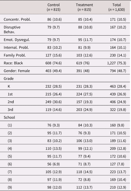
Student behavior, that is concentration problems (C), disruptive behavior (D), emotional dysregulation (E), internalization problems (I), and family problems (F), was assessed with the Teacher Observation of Classroom Adaptation-Checklist (TOCA-C; Koth, Bradshaw, & Leaf, Reference Koth, Bradshaw and Leaf2009). Internal consistency (evaluated via Cronbach's alpha) for the subscales ranged from 0.70 to 0.94. To evaluate potential patterns of students’ problematic behavior, we dichotomized subscale-specific mean composite scores. Problematic behavior was defined as subscale scores at or beyond the 90th sample percentile (0 = TOCA-C subscale score <90th percentile, 1 = TOCA-C subscale score ≥90th percentile). Binary problem behavior indicators were analyzed using MOB CFA with a first-order base model, assuming independence between problem behavior indicators. Gender (0 = male, 1 = female), grade (K-3rd grade), race (1 = black, 0 = others), and school membership were used as splitting variables. Descriptive statistics of all variables for the overall sample and by treatment status are given in Table 1.
Demographic statistics. Values in parentheses give percentages

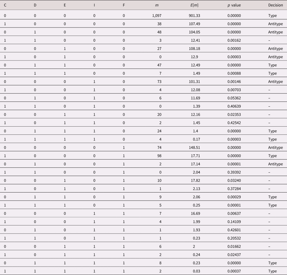
Before using recursive partitioning to find subgroups of problem behavior patterns, we estimate a first-order CFA for the total sample without considering splitting variables as a benchmark. The LR goodness of fit test rejects the model of independence for the total sample (χ2(26) = 809.27, p < .001). Therefore, we expect types and/or antitypes to occur. Table 2 gives the expected frequencies, p values of cell-wise binomial tests, and CFA decisions based on a Bonferroni-corrected significance level of 0.05/32 = 0.00156. Overall, we observe 10 types and seven antitypes. We refrain from a detailed interpretation of these 17 extreme cells. Instead, we highlight some important aspects of the results and use them as a benchmark for comparison with results obtained from first-order MOB CFA. Some aspects of the results in Table 2 are quite typical for CFA. For example, the largest cell describing the absence of any problem behavior {0 0 0 0 0} constitutes a CFA type. Here, 901.3 cases (55.3% of the sample) were expected but 1,097 (67.3%) were observed. The second largest cell, configuration {1 0 0 0 1} describing students with severe concentration problems and family issues, also constitutes a CFA type; about 17.7 (1.2%) were expected and 98 (6.0%) were observed. Interestingly, the third and fourth largest cells in the cross-table determine CFA antitypes. These are the configurations {0 0 0 0 1} (i.e., severe family problems only; expected to be observed in about 148.5 cases [9.1%], but only observed for 74 students [4.5%]) and {0 0 0 1 0} (i.e., internalization problems only; expected for about 101.3 students [6.2%], however, only observed for 73 students [4.5%]). Other important CFA types are the configurations {0 1 1 0 0} and {0 1 1 1 0}. The first one describes students with severe disruptive behavior as well as severe emotional dysregulation which occurred in 47 cases (2.9%). However, according to the independence model, one would expect only 12.5 cases (0.8%). The second configuration describes students with severe disruptive behavior, emotional dysregulation, and internalization problems. Here, only 1.4 cases (0.09%) were expected, but 24 students (1.5%) were observed.
First-order configural frequency analysis (CFA) results for the total sample (n = 1,630)

Note. C = concentration problems, D = disruptive behavior, E = emotional dysregulation, I = internalization problems, F = family problems, m = observed frequencies, E[m] = expected frequencies. Bonferroni-corrected α = 0.00156.
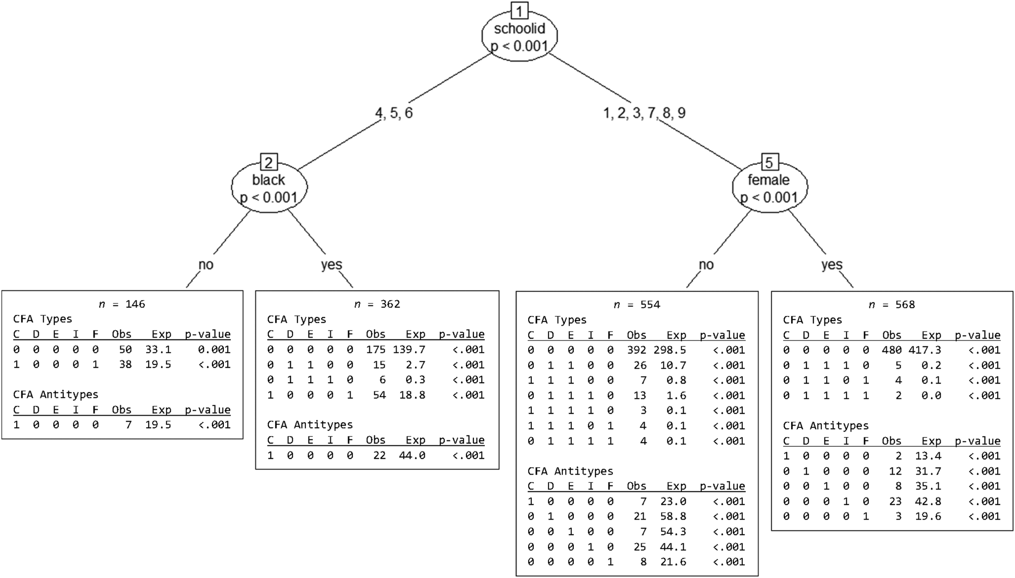
Figure 3 gives the estimated MOB CFA tree using similar specifications as in Simulation Study 1. Three of the four covariates were identified as important splitting variables: school membership, race, and gender. First, MOB separates three schools (Schools 4, 5, and 6) from the remaining six (Schools 1, 2, 3, 7, 8, and 9). Further, in the three separated schools, students’ race constitutes an important moderating factor. In contrast, for the remaining six schools, gender instead of race proves to be an important influence. The estimated tree results in four subgroups (terminal nodes). Subgroup 1 consists of non-black students in Schools 4, 5, 6 (n = 146, 9.0%), Subgroup 2 are black students in the same schools (n = 362, 22.2%), Subgroup 3 describes male students in the Schools 1, 2, 3, 7, 8, and 9 (n = 554, 34.0%), and the last subgroup consists of female students in one of the six schools (n = 568, 34.8%). Each terminal node consists of a separate first-order CFA base model. Bonferroni-corrected binomial tests were used to test whether types or antitypes are present per subgroup. The LR goodness of fit test rejects the model of independence in all four subgroups (LR χ2 statistics ranged from 75.98 to 337.78 with 26 degrees of freedom and all ps < .001). Therefore, as expected, types and antitypes emerge in every subgroup and, more important, type/antitype patterns vary across subgroups where some patterns can be observed in every subgroup and some patterns are unique to specific subgroups. In the following, we interpret some of the results presented in Figure 3 with respect to the occurrence of types/antitypes at the population and subpopulation levels. The type pattern {0 0 0 0 0}, describing the absence of problem behavior, occurs in every subgroup indicating that this is a population type (i.e., one that is observed across all partitions of the sample). Similarly, the antitype pattern {1 0 0 0 0} is also observed in every subgroup and can, thus, be conceptualized as a population antitype. The second largest type for the total sample, {1 0 0 0 1}, is specific to the Subgroups 1 and 2 (i.e., students in the Schools 4, 5, and 6), and, therefore, describes a subpopulation type (i.e., a type that occurs in specific partitions of the data). In other words, the occurrence of severe concentration problems and family issues are specific to the three schools described above. The largest antitype according to the CFA results based on the total sample – family issues only ({0 0 0 0 1}) – is, in fact, specific to Subgroups 3 and 4 and constitutes a subpopulation antitype. In other words, family issues only occur with lower probability than expected in the remaining six schools. This effect does not depend on students’ gender.
Recursively partitioned first-order configural frequency analysis of student problem behavior indicators (C = concentration problems, D = disruptive behavior, E = emotional dysregulation, I = internalization problems, F = family problems) based on n = 1,630 students.

Prediction CFA Trees
P-CFA has been proposed by Lienert and Krauth (Reference Lienert, Krauth and Eckensberger1973) and extended by von Eye and Bogat (Reference von Eye and Bogat2005) and von Eye, Mair, and Bogat (Reference von Eye, Mair and Bogat2005). The main difference between standard CFA and P-CFA concerns the status of the variables involved. In standard CFA (e.g., the first-order CFA discussed above) all variables are treated as exploratory variables. In contrast, in P-CFA one explicitly distinguishes between predictor (independent) and outcome (dependent) variables with the goal to identify predictor patterns that are associated with certain outcomes. Outcomes can come in the form of specific single events (e.g., receiving a clinical diagnosis) or in the form of specific patterns associated with multiple outcome variables (e.g., showing a clinically relevant behavior pattern). Similar to standard CFA, P-CFA does not ask whether predictor variables are related to outcome variables (these types of questions are usually addressed using (multinomial) logistic regression models). Instead, P-CFA asks whether specific patterns of categorical predictors go hand-in-hand with specific outcome patterns (von Eye et al., Reference von Eye, Mair and Bogat2005). To introduce P-CFA, let Y be a binary outcome variable and X 1 and X 2 are two binary predictors. Crossed, the three variables span a 2 × 2 × 2 cross contingency table. The P-CFA base model proposed by Lienert and Krauth (Reference Lienert, Krauth and Eckensberger1973) has the following characteristics: (a) the base model is saturated in the predictor variables (thus, types/antitypes cannot emerge due to the association among predictors), (b) the base model is saturated in the outcome variables (thus, types/antitypes cannot emerge due to the association among outcome variables), and (c) the base model assumes independence between predictor and outcome variables. In other words, types/antitypes can only emerge due to the presence of a predictor–outcome association. Specifically, if, for a specific predictor pattern, more cases are observed than expected under the P-CFA base model, the predictor pattern is said to predict the occurrence of the outcome pattern and, thus, constitutes a prediction type. In contrast, if fewer cases are observed, the predictor pattern is said to predict the nonoccurrence of outcome patterns and constitutes a prediction antitype. For the three variables (Y, X 1, and X 2), the corresponding base model is

with λ being the intercept, $\lambda ^{X_1}$ , $\lambda ^{X_2}$
 , and λ Y being the main effects of the three variables, and $\lambda ^{X_1X_2}$
 specifies the two-way interaction on the predictor side of the model. Terms that are missing in the base model are those that link the predictors (X 1 and X 2) to the outcome Y. The corresponding effect coded design matrix of the model is

where the first column represents the intercept (λ), columns 2–4 indicate the three main effects for X 1, X 2, and Y, and the last column represents the interaction term X 1X 2.
In contrast to standard P-CFA, the proposed P-CFA tree approach assumes that subgroups (g = 1, …, G) exist for which potentially different prediction type/antitype patterns occur. P-CFA types/antitypes that exist for all G subgroups constitute population prediction types/antitypes and types/antitypes that are unique to specific subgroups describe subpopulation prediction types/antitypes. Again, the P-CFA tree is constructed using a priori specified splitting variables which can be categorical or continuous in nature. Formally, for three binary variables (X 1, X 2, and Y), the MOB P-CFA model for g = 1, …, G subgroups can be written as

with λ g representing the subgroup-specific intercept, $\lambda _g^{X_1}$ , $\lambda _g^{X_2}$
 , $\lambda _g^Y$
 referring to the subgroup-specific main effects, and $\lambda _g^{X_1X_2}$
 being the subgroup-specific interaction effect. Because log-linear model parameters are allowed to vary across subgroups, the algorithm is able to identify subgroup-specific prediction types and antitypes. To implement MOB P-CFA, one requires a case-wise design matrix. Consider two individuals, three binary variables (two predictors X 1 and X 2 and one outcome Y; 0 = event not observed, 1 = event observed), and two continuous splitting variables U and V. For Person 1, suppose we observe X 1 = X 2 = Y = 1, that is the configuration {1 1 1}, together with U = u 1 and V = v 1. For Person 2, we observe the configuration {0 1 0} and U = u 2 and V = v 2. Then, the corresponding case-wise design matrix for the two participants is (the intercept is implied in the model matrix)

with m being the observed frequencies for all possible patterns. For Person 1, one uses m = 1 for the observed pattern {1 1 1} and m = 0 for the remaining configurations. In a similar fashion, for Person 2, one uses m = 1 for the configuration {0 1 0} and m = 0 otherwise. Similar to the first-order MOB CFA described above, values of the splitting values U and V are each repeated eight times for each person. To estimate the MOB P-CFA, one uses a MOB Poisson regression model where m serves as the response, the four dummy variables for X 1, X 2, Y, and X 1X 2 are the independent variables, and U and V serve as MOB splitting variables. Again, generalized M-fluctuation tests (Zeileis & Hornik, Reference Zeileis and Hornik2007) are used to detect instabilities of model parameters along the splitting variables. Parameter instabilities are captured by fitting separate Poisson regression models per subgroup. The resulting partitions represent terminal nodes of a P-CFA tree. Each terminal node contains a separate P-CFA model with partition-specific parameters and (potentially) prediction types and antitypes. To evaluate the performance of MOB P-CFA, we performed a second Monte Carlo simulation experiment.
Simulation Study 2
In the second Monte Carlo simulation experiment, we focus on a data scenario in which both, a variable- and a person-oriented effect exist simultaneously. Specifically, we focus on a pre–post comparison for two experimental groups, a treatment group and a business as usual group, and a binary outcome variable Y (0 = event not observed, 1 = event observed). The data-generating mechanism followed a logistic regression model with one outcome and two predictors, that is, log(p/[1 − p]) = β0 + β1T + β2X with p being the probability of the event occurring (Y = 1), T being a treatment indicator (0 = business as usual, 1 = treatment), and X being a continuous covariate (representing continuous pre-treatment scores). T was randomly drawn from a binomial distribution with a probability of T = 1 of 50% and X was generated from a standard normal distribution. Mimicking properties of a successful random assignment of subjects to either the control or treatment group, T and X were generated independently with Cor(T, X) = 0. Following Huang (Reference Huang2019), the intercept β0 was set to zero (representing the predicted probability in the reference group of 50%), the treatment effect was set to β1 = 0.5, and the covariate effect was β2 = 1. The outcome was sampled from a Bernoulli distribution with probability p = exp(β0 + β1T + β2X)/[1 + exp(β0 + β1T + β2X)].
Data were generated using the same regression tree as in Simulation Study 1 (cf. Figure 1). That is, four subgroups were simulated using the three partitioning variables Z 1, Z 2, and Z 5 among a set of ncov covariates. The overall number of covariates was ncov = 5 or 10. Because P-CFA assumes that variables are categorical in nature, the continuous X variable was dichotomized at the mean. In the first subgroup (i.e., if Z 1 ≤ 17 and Z 2 ≤ 30), observed configuration of X, T, and Y were replaced with the type configuration {1 1 1} with probabilities δ = 0.20, 0.25, 0.30, and 0.35. In the second and third subgroups (i.e., if Z 1 > 17 and Z 2 ≤ 30 or if Z 2 > 30 and Z 5 ≤ 63) no types occurred. In the fourth subgroup (Z 2 > 30 and Z 5 > 63), the type configuration was {0 1 1} occurred with probability δ. In other words, in Subgroup 1, the occurrence of Y = 1 is associated with T = 1 and X = 1 (i.e., X scores above the sample mean) which is also in line with the overall variable-oriented effect (i.e., large X scores and T = 1 increase the chance of Y = 1). In contrast, in Subgroup 4, Y = 1 is likely to occur together with T = 1 and X = 0 (i.e., X scores below the sample mean). Note that the latter person-oriented effect contradicts the global variable-oriented effect. Here, lower X scores and T = 1 is likely to be observed together with Y = 1. Overall sample sizes were set to n = 500, 1,000, and 1,500. The simulation design was fully crossed resulting in 2 (number of covariates) × 3 (sample size) × 4 (effect size δ) = 24 simulation conditions. One hundred samples were generated per condition.
For each sample, the case-specific design matrix of the P-CFA was generated to predict the observed configuration frequencies. Next, MOB was employed to identify P-CFA subgroups. MOB estimation was based on a GLM tree with a log link and a Poisson error distribution. The variables Z 1, …, Zncov were used as potential splitting variables. Bonferroni-corrected parameter stability tests were performed with a familywise nominal significance level of 5%. Similar to Simulation Study 1, regression trees were estimated with a maximal depth of three, limiting the number of terminal nodes to eight. Finally, for each identified subgroup, we estimated a separate P-CFA with Bonferroni-corrected binomial tests to test for the presence of prediction types and antitypes.
Results
Figure 4 summarizes the performance of the MOB P-CFA approach as a function of sample size, number of covariates, and probability of CFA types (δ). The upper panel of Figure 4 gives the average tree size per simulation condition, the lower panel summarizes tree accuracy (using the same definition as in Simulation Study 1). For smaller sample sizes and δ effects, the estimated trees tend to be smaller than the “true” tree structure. However, for large samples and δ ≥ 0.30, the average tree size is close to the “true” value. For n = 500, 1,000, and 1,500, we observe average tree sizes of 4.03 (SD = 1.35), 5.44 (SD = 1.53), and 6.08 (SD = 1.34) for ncov = 5, and 3.94 (SD = 1.37), 5.33 (SD = 1.62), and 6.13 (SD = 1.35) for ncov = 10. Similarly, large sample sizes (n = 1,500) and larger δ effects (δ ≥ 0.30) are required to obtain tree accuracy rates larger than 80% (see Figure 4 lower panel). Overall, we conclude that, similar to the first-order MOB CFA, MOB P-CFA is able to identify the underlying data-generating tree structure. However, again, larger samples are preferable when studying P-CFA tree structures.
Average tree size and accuracy of recursively partitioned prediction configural frequency analysis (P-CFA) as a function of sample size (n), number of covariates (ncov), and probability of CFA types (δ).

Finally, we now focus on the percentage of correctly identified prediction types per subgroup. Again, we restrict our analysis to cases in which the MOB P-CFA algorithm correctly identified four subgroups. For Subgroup 1, we focus on the percentages to detect the prediction type {1 1 1}; for subgroup 4, we focus on the configuration {0 1 1}. Percentages to correctly identify {1 1 1} as a CFA type of Subgroup 1 ranged from 33.3% to 100% across all simulation conditions with an average of 89.5% (SD = 18.4%). Note that percentages larger than 80% were observed for 19 out of 24 simulation conditions. The remaining five simulation conditions describe data scenarios involving small sample sizes and small δ effects. For example, the minimum of 33.3% occurred for n = 500, δ = 0.25, and ncov = 5. Percentages of correctly identifying {0 1 1} as a CFA type in Subgroup 4 were lower than the corresponding percentages in Subgroup 1. This can be explained by the fact that the configuration {0 1 1} contradicts the underlying variable-oriented effect. Large percentages were only observed for n = 1,500 and δ = 0.35. Here, for ncov = 5, {0 1 1} was correctly identified in 80.8% of the cases; for ncov = 10, the type configuration was detected in 73.0% of the cases. Thus, overall, we can conclude that MOB P-CFA is able to detect subgroup-specific prediction types. Detection, however, is more accurate for type configurations that are in line with the global variable-oriented effect (such as {1 1 1} in the present context). When prediction type patterns contradict the global variable-oriented effect (such as {0 1 1}), large samples and large δ effects are required to detect these patterns with sufficient accuracy.
Empirical Example 2
In the following section, we illustrate the application of the MOB P-CFA approach again using the IY TCM data from Reinke et al. (Reference Reinke, Herman and Dong2018). Now, we focus on the effectiveness of the IY TCM program to reduce teacher-rated internalization problems of students. Pre- and post-treatment internalization problems were measured using the TOCA-C (Koth et al., Reference Koth, Bradshaw and Leaf2009). Scores were dichotomized at the 90th percentile. The binary internalization indicators were then analyzed using MOB P-CFA. Treatment status (T; 0 = business as usual; 1 = IY TCM) and pre-treatment internalization status (I 1; 0 = <90th percentile; 1 = ≥90th percentile) were used as predictors and post-treatment internalization problems (I 2; 0 = <90th percentile; 1 = ≥90th percentile) was treated as outcome variable. The corresponding base model was saturated in the predictors and assumed independence between outcome and predictors. Formally, the model can be written as $\log \lpar {E[ m ] } \rpar = {\rm \lambda } + {\rm \lambda }^{I_1} + {\rm \lambda }^T + {\rm \lambda }^{I_2} + {\rm \lambda }^{I_1T}$ . The covariates gender (0 = male, 1 = female), grade (K-3rd grade), race (1 = black, 0 = others), and school membership were used as splitting variables in the MOB algorithm.
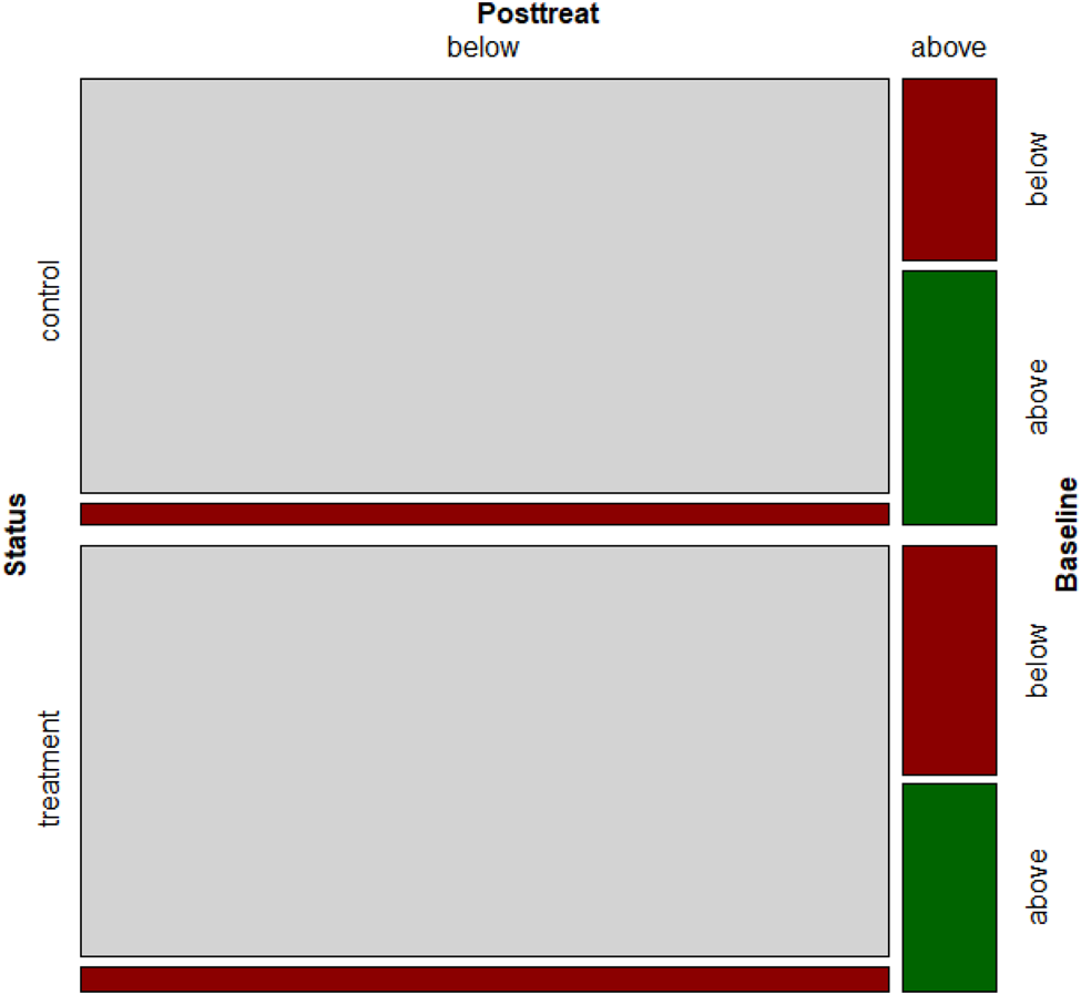
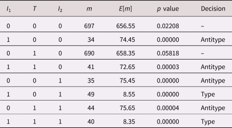
First, we again focus on the P-CFA results of the total sample of 1,630 students given in Table 3 (the corresponding mosaic display is given in Figure 5). According to the LR goodness-of-fit test, the model does not fit the data well (χ2(3) = 244.68, p < .001) and we can conclude that prediction types/antitypes may exist. Again, we use the binomial test to evaluate whether cell frequencies significantly deviate from expectation. We used Bonferroni correction to protect the nominal significance level leading to an adjusted significance level of 0.05/8 = 0.00625. Overall, we observe two prediction types and four prediction antitypes. Interestingly, the two largest cells describing the absence of internalization problems in both treatment groups ({0 0 0} and {0 1 0}) do not deviate from expectation under the P-CFA model. Prediction types describe patterns of continuing internalization problems for both experimental groups. For the control group, that is for the cell {1 0 1}, we observed 49 (3.0%) students although only 8.6 (0.5%) had been expected. In the treatment condition, we observed 40 (2.5%) students with pre- and post-treatment internalization problems while only expecting 8.4 (0.5%) cases. The first two out of the four prediction antitypes, {1 0 0} and {1 1 0}, describe decreasing internalization problems in both groups. Here, only 34 cases (2.1%) were observed in the control group but 74.5 (4.6%) had been expected. Similarly, in the treatment group, 41 cases (2.5%) have been observed and 72.7 (4.5%) had been expected. Finally, the last two prediction antitypes describe an increase of internalization problems for both groups, {0 0 1} and {0 1 1}. Thirty-five control participants (2.2%) have been observed but 75.5 (4.6%) had been expected. In the treatment group, 44 students (2.7%) showed this pattern while 75.7 (4.6%) should have been observed according to the base P-CFA model.
Mosaic plot of teacher-rated internalization problems for the total sample (n = 1,630 students); Status (left dimension) = control versus Incredible Years Teacher Classroom Management (IY TCM) treatment, posttreat (top dimension) = post-treatment internalization problems, baseline (right dimension) = pre-treatment internalization problems; red = configural frequency analysis (CFA) antitype, green = CFA type, gray = no deviation from expectation.

Prediction configural frequency analysis (P-CFA) results for the total sample (n = 1,630)

Note. I 1 = pre-treatment internalization problems, I2 = post-treatment internalization problems, m = observed frequencies, E[m] = expected frequencies. Bonferroni-corrected α = 0.00625.
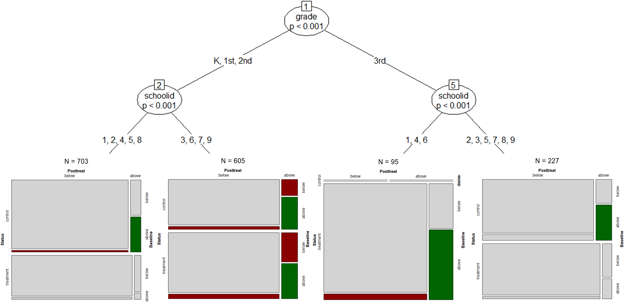
Next, we ask whether the existing prediction types/antitypes hold on the population level or whether some prediction types/antitypes are specific to certain subpopulations. In addition, we evaluate whether the two patterns that did not significantly deviate from model expectation constitute prediction types/antitypes in a subpopulation. The MOB P-CFA algorithm can be used to address both questions. Figure 6 summarizes the MOB P-CFA tree for the splitting variables gender, grade, race, and school membership. Out of the four splitting variables two proved to be useful to partition the data, grade and school membership. Note that school membership was selected as a splitting variable for both grade partitions. Thus, the resulting regression tree consists of four terminal nodes. The first subgroup (n = 703, 43.1%) consists of K-, first- or second-grade students in Schools 1, 2, 4, 5, or 8. Students in the second subgroup (n = 605, 37.1%) are in K-, first, or second grade in Schools 3, 6, 7, or 9. The third subgroup is characterized as third-grade students in Schools 1, 4, or 6 (n = 95, 5.8%), and the last subgroup consists of third-grade students in Schools 2, 3, 5, 7, 8 or 9 (n = 227, 13.9%). For all four subgroups Bonferroni-corrected binomial tests suggest that types/antitypes exist.
MOB P-CFA tree of teacher-rated internalization problems based on n = 1,630 students. Status (left dimension) = control versus Incredible Years Teacher Classroom Management (IY TCM) treatment, posttreat (top dimension) = post-treatment internalization problems, baseline (right dimension) = pre-treatment internalization problems; red = CFA antitype, green = CFA type, gray = no deviation from expectation.

In contrast to Empirical Example 1, we use mosaic displays to summarize end nodes (cf. Figure 6). In the mosaic plots, we use green areas to indicate P-CFA types, red areas to indicate P-CFA antitypes, and gray areas when no significant discrepancies exist. First, in comparison with the mosaic plot for the total sample (Figure 5), only Subgroup 2 shows similar dependency structures (interestingly, this is not the largest subgroup in the sample). Next, we observe different mosaic structures and, therefore, different dependencies between variables, across partitions, as expected. Overall, we observe the same type/antitype patterns as for the total sample. That is, using the order {baseline, status, post-treatment} to indicate baseline internalization problems (0 = below, 1 = above), status (0 = control, 1 = IY TCM treatment), and post-treatment internalization problems (0 = below, 1 = above), the configurations {1 0 1} and {1 1 1} constitute CFA types and {1 0 0}, {1 1 0}, {0 0 1}, and {0 1 1} are CFA antitypes. None of these patterns, however, hold on a population level. The type pattern {1 0 1} for example (i.e., high baseline scores – control group – high post-treatment scores), holds for the subpopulation of Subgroups 1, 2 and 4, and the CFA type {1 1 1} (high baseline scores – IY TCM treatment – high post-treatment scores) is only observed for Subgroups 2 and 3. Similarly, the antitype {1 0 0} (high baseline scores – control group – low post-treatment scores) holds in Subgroups 1 and 2, {1 1 0} is only observed in Subgroups 2 and 3, and {0 0 1} and {0 1 1} only exists in Subgroup 2.
Evaluating the Stability of CFA Trees
Tree structures found in the data can be unstable and highly sample dependent, that is, small changes in the input data can have tremendous effects on the resulting tree structure (Philipp, Rusch, Hornik, & Strobl, Reference Philipp, Rusch, Hornik and Strobl2018). Thus, carefully evaluating the stability of a regression tree constitutes an important element of every MOB application. Nonparametric bootstrapping has for example been suggested to quantify the robustness of the initial tree results (Philipp et al., Reference Philipp, Rusch, Hornik and Strobl2018). Because different tree structures can lead to equivalent partitions and interpretation (Turney, Reference Turney1995), instead of evaluating the structure of re-sampled trees, one can focus on two elements of a tree: (a) variable selection and (b) cut-point selection.
Let b = 1, …, B denote the index of the B bootstrap samples (i.e., sampling with replacement from the original data) and j = 1, …, J indicates the variables (Zj) considered for partition. Further, let sbj be an indicator that takes value 1 if Zj is selected for partitioning and 0 otherwise. Then, the variable selection percentage is defined as $B^{{-}1}\sum\nolimits_b {s_{bj} \times 100}$ and is expected to be close to 100% for those partitioning variables that had been selected in the original tree. To evaluate potential variability of cut-points, two strategies are available depending on the measurement scale of the partitioning variable Zj. For categorical splitting variables, cut-point selection percentages of the B re-samples can be used. In case of a continuous splitting variable, descriptive statistics such as means and standard deviations can be used to summarize the distribution of cut-points obtained from B re-samples (e.g., average cut-points of Zj are expected to be close to the corresponding cut-point in the initial tree).
To illustrate MOB stability analysis in the context of configural frequency trees, we again use the data of the two empirical examples. For the first data example, we generated 100 re-samples of the five baseline student behavior indicators (concentration problem, disruptive behavior, emotional dysregulation, internalization problems, and family problems) and estimated a first-order MOB CFA for each re-sample. In line with the initial tree (cf. Figure 3), school membership was selected in 100% of the re-samples. Race was selecting in 57% and gender was selected in 38% of the re-samples. In addition, grade was identified as being a relevant splitting variable in 12% of the re-samples. In other words, with respect to the stability of the initial configural frequency tree, we observe mixed results. While school membership is identified as a stable component of the trees, race and gender show instabilities. Further, cut-point selection analysis of school membership suggests that the observed partition in Figure 3, [4, 5, 6] and [1, 2, 3, 7, 8, 9] was replicated in 68% of the re-samples. However, the most prevalent school membership partition (replicated in 82% of the re-samples) was one where School 6 is member of the other partition, that is, [4, 5][1, 2, 3, 6, 7, 8, 9]. This indicates that partitioning can be considered stable for Schools 4 and 5, but selection variability exists for School 6.
For the second data example, we generated 100 re-samples using pre- and post-treatment internalization and treatment status indicators. For each re-sample, we used MOB P-CFA to detect potential subgroups. The two splitting variables of the initial tree (school membership and grade) were selected in 100% of the re-samples indicating that, in contrast to the tree in Example 1, this configural frequency tree can be considered stable (note that, in addition, gender was selected as a splitting variable in 3% of the re-samples). Further, cut-point analysis suggests that in the majority of re-samples (68%) MOB P-CFA separated K-, first and second graders from third graders (which is in line with the initial tree), followed by partitions of the form [K, 3rd][1st, 2nd] (18%) and [K, 1st, 3rd][2nd] (17%). Further, the two school membership partitions of the initial tree, that is, [1, 2, 4, 5, 8][3, 6, 7, 9] for K-, first, and second graders and [1, 4, 6][2, 3, 5, 7, 8, 9] for third graders was selected in the majority of re-samples (27% and 24% respectively), followed by the partitions [1, 2, 3, 4, 5, 7, 8][6, 9] (22%). The remaining partitions were less likely to occur (all ≤8%). Thus, overall, we can conclude that the initial configural frequency tree is sufficiently stable with respect to the selected cut-points.
Discussion
The present study introduced principles of configural frequency modeling and recursive partitioning and proposed a combination of the two methods to study moderation processes from a person-oriented (i.e., a pattern) perspective. CFA identifies the location of a categorical data space for which effects can be observed and MOB identifies subgroups for which model parameters significantly vary. Combining the two approaches leads to a powerful algorithm to evaluate moderation processes while preserving a person-oriented perspective. Configural frequency trees can be used to identify population-level and subpopulation-level types and antitypes. Application of the proposed configural frequency tree framework was illustrated focusing on first-order CFA and P-CFA trees. For both applications, Monte Carlo simulation results suggested that MOB CFA is able to recover true tree structures with adequate probability in particular for large sample sizes and large effect sizes. Further, two real-world empirical examples from school mental health research were presented for illustrative purposes. In both examples, MOB CFA identified four subgroups (partitions) that differ with respect to the likelihood of observing specific CFA type/antitype patterns.
The findings highlight the promise of CFA for identifying meaningful heterogeneity within populations and in response to interventions. The empirical example identified common patterns of youth behavior problems in relation to their expected occurrence. Youth with no behavior problems and those with co-occurring problems (concentration and family problems as well as emotional dysregulation and disruptive behaviors with and without internalization) were over-represented types. Those with family problems alone and internalization problems alone emerged as underrepresented antitypes. These findings are consistent with extensive research showing the common co-occurrence of youth behavior problems which arise rarely in isolation or as singular symptoms (Angold, Costello, & Erkanli, Reference Angold, Costello and Erkanli1999; Herman, Ostrander, Walkup, Silva, & March, Reference Herman, Ostrander, Walkup, Silva and March2007). For instance, one study found that 80% of youth with major depressive disorder had clinically significant levels of other symptoms including concentration problems and disruptive behaviors (Herman et al., Reference Herman, Ostrander, Walkup, Silva and March2007). In addition, much prior research has highlighted family problems as a strong risk factor for youth mental health concerns (Dishion & Patterson, Reference Dishion, Patterson, Cicchetti and Cohen2006; George, Herman, & Ostrander, Reference George, Herman and Ostrander2006; Rothenberg, Hussong, & Chassin, Reference Rothenberg, Hussong and Chassin2016), so it is not surprising that an antitype of family problems without youth behavior problems emerged from these analyses. CFA offers a parsimonious method for characterizing patterns of co-occurring symptoms, environmental contexts, and timing of risk conditions in line with a developmental psychopathology perspective (Cicchetti & Toth, Reference Cicchetti, Toth, Cicchetti and Cohen1995).
Subsequent analyses that included school, race, and gender as partitioning variables, suggested that particular schools were associated with higher risk for youth behavior problems, especially the concentration plus family problems type. School contexts influence student risk and how family risk (e.g., the percentage of families with economic challenges) intersects with school risk to influence negative youth outcomes (Biglan, Flay, Embry, & Sandler, Reference Biglan, Flay, Embry and Sandler2012; Reinke & Herman, Reference Reinke and Herman2002). That the family-only antitype was most common in the other six schools is consistent with the importance of school context in the likelihood of youth expressing emotional and behavior symptoms. These schools may have provided a protective buffer for youth in them that reduced their risk of mental health concerns, at least as observed and reported by their teachers, in the presence of family problems. It was also noteworthy that the “no problems” pattern emerged as an overrepresented population type, again suggesting that the collective school environment in this district may have provided a protective buffer that mitigated expected levels of youth mental health concerns.
The CFA of treatment effects highlights the promise of the method in uncovering contextual factors associated with youth outcomes in response to intervention that does not have the downside or complexities of using multiple moderation analyses. In this example, both treatment conditions experienced comparable trends. MOB findings highlight the promise of CFA in helping understanding the generalizability and replication of RCT findings. Recent research has suggested that treatment effects may be contingent on unspecified and unexamined contextual factors that are inherent to any study. For instance, Kaplan et al. (Reference Kaplan, Cromley, Perez, Dai, Mara and Balsai2020) conducted a multisite study that involved 10 RCTs of the same design and found widely discrepant effect sizes based on the context of each study. These authors argued that causal mechanisms need to be contextualized and that future studies need to include careful elaboration and evaluation of potential contextual moderators of study effects. Recently, Herman, Dong, Reinke, and Bradshaw (Reference Herman, Dong, Reinke and Bradshaw2020) also found the findings of an educational RCT varied before and after a prominent historical event based on both participant race and treatment condition. Both Kaplan et al. (Reference Kaplan, Cromley, Perez, Dai, Mara and Balsai2020) and Herman et al. (Reference Herman, Dong, Reinke and Bradshaw2020) used moderation analyses to identify these contextual variations of study effects. MOB CFA offers a more sophisticated and powerful tool to detect and summarize multiple contextual processes simultaneously.
The presented MOB CFA framework can be extended in various ways. In essence, any CFA model that can be cast as a log-linear model can serve as a candidate for MOB CFA. Here, we want to focus on two potential extensions that seem particularly relevant for developmental psychopathology: k-sample CFA and longitudinal CFA. k-sample CFA has been suggested to test whether configurations of categorical variables (so-called discrimination variables) differ across the categories of a grouping variable. In this approach, the grouping variable can be considered a moderator. MOB CFA could be used to investigate the effects that additional continuous or categorical moderators have, and to determine whether population-based group differences hold when additional moderators are the basis of finer-grained classifications. Similarly, longitudinal CFA can be used to determine whether patterns of development are predictive of endpoints of development. Here, MOB CFA can be used to find finer-grained endpoint patterns as well as finer-grained developmental trajectories. In other words, MOB CFA can be used to determine whether a population is homogeneous in type/antitype patterns of development.
Another extension concerns sensitivity analyses associated with MOB CFA applications. Previous studies have emphasized that single decision trees can provide low predictive performance and that ensemble techniques such as bagging (Breiman, Reference Breiman1996), boosting (Freund & Schapire, Reference Freund and Schapire1995), and random forests (Breiman, Reference Breiman2001) can overcome some of these issues (Fokkema & Strobl, Reference Fokkema and Strobl2020; Strobl et al., Reference Strobl, Malley and Tutz2009). We expect that making use of ensemble methods in the context of MOB CFA can also lead to model improvements.
Although CFA is usually presented for “true” categorical variables, that is, variables that measure constructs in the form of (un)ordered distinct categories (taxa), configural frequency modeling can also be useful in the context of categorized continuous variables (e.g., a dichotomized composite measure) leading to a broad area of potential applications in developmental psychopathology research. In the presented real-world data examples, for instance, composite measures of student behavior were dichotomized at the 90th percentile to indicate problem behavior. It is important to note that data categorization is not free of limitations and has been hotly debated in quantitative methods research. Some authors argue that dichotomization should be avoided due to the tremendous loss of information affecting the validity of subsequent statistical models (Cohen, Reference Cohen1983; DeCoster, Iselin, & Gallucci, Reference DeCoster, Iselin and Gallucci2009; MacCallum, Zhang, Preacher, & Rucker, Reference MacCallum, Zhang, Preacher and Rucker2002; Maxwell & Delaney, Reference Maxwell and Delaney1993; Rucker, McShane, & Preacher, Reference Rucker, McShane and Preacher2015), others argue that the cost of dichotomization is comparatively low given potential benefits in clarity and communicability of results (Iacobucci, Posavac, Kardes, Schneider, & Popovich, Reference Iacobucci, Posavac, Kardes, Schneider and Popovich2015; von Eye & Mair, Reference von Eye, Mair, Barragan, Martínez, Barajas and Covarrubias2012; Westfall, Reference Westfall2011; Wiedermann & von Eye, Reference Wiedermann and von Eye2020a). Furthermore, and most important for the present context, all previous studies have discussed benefits and costs of dichotomization from a purely variable-oriented perspective. Less is known about the effects of dichotomization when research hypotheses are tested in terms of patterns, that is, in the person-oriented research context. Although further studies are needed to evaluate the gains and losses of data categorization in person-oriented analyses, our results of Simulation Study 2 may provide some preliminary insights. In the second simulation experiment, we simulated a continuous covariate that was subsequently dichotomized at the mean. Simulation results indicate that MOB identifies underlying partitions with high accuracy even when a dichotomized variable is included in the model. Thus, in the present context, adverse effects of categorization can be expected to be low in configural frequency modeling.
MOB CFA does not come without some limitations. Both simulation studies suggested that large sample sizes are preferable to detect tree structures. The requirement of sufficiently large sample sizes will often be fulfilled in cross-sectional research that adopts a person-oriented/pattern perspective. In precision public health and precision prevention science (Khoury, Iademarco, & Riley, Reference Khoury, Iademarco and Riley2016; Supplee, Parekh, & Johnson, Reference Supplee, Parekh and Johnson2018), for example, it is well-recognized that large samples are needed to take individual variability into account and to make valid statements about subgroups or clients. That is, since collected information of people is more informative when diverse people of the underlying population are included and large enough subgroup-specific sample sizes are necessary to guarantee an accurate representation of the corresponding subpopulation, the overall sample sizes can be expected to be sufficiently large for applying MOB CFA. However, often, person-oriented studies focus on intensive longitudinal individual data (e.g., daily diary data) with moderate samples sizes. Configural frequency modeling of intensive longitudinal data has been discussed by von Eye et al. (Reference von Eye, Mair and Mun2010). Here, CFA models are available to evaluate runs (asking whether adjacent scores are equal or different) and lags of a series (e.g., relating information from one time point to information from the next). Information that describes runs and lags can then be categorized and crossed with other categorial indicators (e.g., demographic variables). The benefit of ideographic data information usually comes at the cost of small to moderate sample sizes. Although, our simulation studies clearly indicated that, in a cross-sectional data setting, large samples are preferable, the ability of MOB CFA to detect heterogenous subgroups will also depend on the complexity of the tree and the magnitude of the effects. For example, extreme groups may also be detectable in the form of a two-group MOB solution even when sample sizes are moderate – apparently, ultimate statements about the performance of MOB CFA under such extreme conditions require further studies.
The requirement of larger sample sizes also puts constraints on the number of variables that can be incorporated to define configurations of interest. For example, with 1,500 subjects and 10 binary variables the case-wise data for MOB has 210 × 1,500 = 1,536,000 rows. Thus, if the number of indicators is large, researchers should consider the application of a data reduction method prior to MOB CFA. For example, latent class analysis techniques (Collins & Lanza, Reference Collins and Lanza2010; Lazarsfeld & Henry, Reference Lazarsfeld and Henry1968) can be used to summarize potentially complex profiles of subgroups of indicators in the form of a small number of latent classes. Latent class membership information across subgroups of indicators can then be used for recursive partitioning (for a discussion of latent class analysis in the context of CFA modeling see Wiedermann & von Eye, Reference Wiedermann and von Eye2016).
Overall, MOB CFA can be a powerful tool to study moderation processes from a pattern perspective provided that sample sizes are sufficiently large, and one takes effort in critically evaluating the robustness of the findings. To make MOB CFA accessible to researchers, we provide an implementation of the discussed models in R in the online supplement to this article.
Supplementary Material
The supplementary material for this article can be found at https://doi.org/10.1017/S0954579421000018.
Financial Statement
This work was supported by the US Department of Education, Institute of Education Sciences (KH and WR, grant number R305A100342).
Conflicts of Interest
None.