1. INTRODUCTION
The task of modeling multivariate distributions has always been
challenging. For this reason, it is very common to use elliptic
distributions because of the fact that these are simple to
characterize. However, in many cases of interest in economics, it is
found that this simple characterization contrasts with empirical
evidence. A typical example is returns distributions in financial
economics and the complex range of dependence that they exhibit. Among
many references, the reader should look at Embrechts, McNeil, and
Straumann (1999).
When dealing with vectors of random variables, the copula function
becomes a very useful object because it allows us to model the
dependence between the variables separately from their marginals. In
practice we may have a clear idea of what the marginals are, although
knowledge of their joint dependence could be limited. Therefore, being
able to use a two-step procedure may be advantageous. Further, computer
estimation can be speeded up. Though this may result in a loss of
efficiency, corrections for the estimators have been proposed (e.g.,
White, 1994).
For example, in the first step we may model unconditional marginal
distributions or may model conditional distributions as in the case of
generalized autoregressive conditional heteroskedasticity (GARCH)
models. Then, cross dependence of the marginal distributions could be
modeled in the second step. The same approach is valid in the case of
stationary time series when we want to model their joint distribution
given their unconditional marginals (when the series is Markovian, see
Darsow, Nguyen, and Olsen, 1992).
Although the copula function is a fairly new concept in econometrics,
there has been growing interest in financial econometrics (Hu, 2002; Bouyé, Gaussel,
and Salmon, 2001; Patton, 2001; Rockinger and Jondeau, 2001; Longin and Solnik, 2001). The last authors deal
with multivariate extreme value theory in the context of financial
assets and use a dependence function equivalent to the copula function.
The copula has been considered elsewhere for studying extreme values
(for a list of extreme value copulas, see Joe,
1997).
We introduce a family of copulas defined in terms of Bernstein
polynomials. We call a copula from this family a Bernstein copula (BC).
After defining a new class of copulas, we show how the BC can be used
as an approximation to known and unknown copulas. When the
approximation is used as an approximation for known copulas, we call it
the approximate Bernstein copula (ABC) representation. This new
representation leads to a general approach in estimation and also to
simplification of many operations whenever a parametric copula is
given. Moreover, for parametric copulas, the Bernstein representation
is useful in studying properties of the copula function itself. When
the same approach is used to approximate unknown copulas, we call this
the empirical Bernstein copula (EBC).
There are many possible representations of continuous functions in
terms of polynomials: e.g., Hermite polynomials (the Edgeworth
expansion) and Padé approximations (the extended rational
polynomials in Phillips, 1982, 1983). However, none of these polynomial
representations share the same properties of Bernstein polynomials in
the context of the copula function. It is important that Bernstein
polynomials are closed under differentiation; for simple restrictions
on the coefficients they always lead to a proper copula function, and
when used as empirical estimators, they have lower variance than
commonly used nonparametric estimators.
The plan for the paper is as follows. Section 2 introduces the BC and
derives some of its mathematical and statistical properties. In Section
3 we introduce the important extension of the Bernstein representation
of given copulas. Issues related to making the polynomial
representation operational are considered in Section 4, where, as
mentioned previously, it is shown that empirical estimation of the BC
density has remarkably good properties in terms of its asymptotic
variance. Moreover, a short simulation is provided to highlight some of
the theoretical results in a finite sample. Other estimation procedures
are possible, and we discuss some, but by no means all, of the issues
in Section 5. Proofs of some results appear in the Appendix.
2. THE BERNSTEIN COPULA
We first recall Sklar's representation for multivariate
distributions. Let H be a k-dimensional distribution
function with one-dimensional marginals
F1,…,Fk; then
there exists a function C from the unit k-cube to the
unit interval such that
Here C is referred to as the k-copula. If each
Fj is continuous, the copula is unique.
For more details see Sklar (1973).
We list some properties of the copula function C.
(1) C is nondecreasing in all its
arguments;
(2) C satisfies the Fréchet bounds
which implies that C is grounded: i.e.,
C(u1,…,uk)
= 0 if uj = 0 for at least one j, and
C(1,…,1,uj,1,…,1) =
uj, ∀j;
(3)
is a copula for independent random
variables, which is called the product copula;
(4) C is Lipschitz with constant one;
i.e.,
Properties (1) and (2) are necessary and sufficient for the
definition of the copula function.
Let α(v1
/m1,…,vk
/mk) be a real-valued constant indexed
by (v1,…,vk),
such that
.
We could also use
αv1,…,vk,
0 ≤ vj ≤
mj, ∀j. Let
Define the following map, CB :
[0,1]k → [0,1], where
Under specific conditions on α(v1
/m1,…,vk
/mk), (2) can be shown to be a copula.
In particular, (2) is defined in terms of k-dimensional
Bernstein polynomials. We state the following definition.
DEFINITION 1. A Bernstein polynomial approximation to f
∈ C[0,1]k
(C[0,1]k is the
space of continuous bounded functions on
[0,1]k) is obtained by applying a linear
operator Bmk to
f ∈
C[0,1]k such
that
or in the more general singular integral representation via the
Stieltjes integral,
for the kernel
which is constant for v/m ≤ t <
(v + 1)/m and has jumps of
at points
t = v/m.
The singular integral representation establishes some clear parallels
to kernel density estimation in statistics. One important property of
multivariate Bernstein polynomials is given next (e.g., DeVore and Lorentz, 1993, p. 10).
LEMMA 1. Let
C[0,1]k be the space of
bounded continuous functions in the k-dimensional hypercube
[0,1]k. Then, the set of Bernstein
polynomials defined in (3) is dense in
C[0,1]k.
Further, the derivatives of a Bernstein polynomial approximation
converge to the approximand whenever this is differentiable (see, e.g.,
(12) and (13), which follow). This concept and its usefulness will
become clear in Section 2.2.
Throughout the paper, we reserve the symbols
CB, Cn, and
C for the BC, the empirical copula based on n
observations, and a general copula, respectively, and use
cB for the BC density; definitions will be
given in due course. The letters m and n will only be
used to define the order of polynomial and the sample size,
respectively.
2.1. The Definition of Bernstein Copula
To restrict (2) to be a copula function, we need to impose some
conditions on α(v1
/m1,…,vk
/mk).
THEOREM 1.
CB(u1,…,uk)
is a copula function if
letting 0 ≤ vj ≤
mj − 1, j =
1,…,k, and
in particular
and
Proof. See the Appendix. █
As a result of (7) in Theorem 1, we could take 1 ≤
vj ≤ mj,
∀j, in (2). Theorem 1 gives sufficient conditions that
are necessary only if m → ∞.
Therefore, we can define the object to be studied in this paper.
DEFINITION 2. If α(v1
/m1,…,vk
/mk) satisfies (5) and (6), we call
CB(u1,…,uk)
in (2) the BC.
From Theorem 1 we see that a BC is a genuine copula, and by Lemma 1,
we know that the BC may serve as an approximation to a given arbitrary
parametric copula. By the properties of Bernstein polynomials, the
coefficients of the BC have a direct interpretation as the points of
some arbitrary approximated copula. In this approach, we use the terms
ABC or EBC (see Sections 3 and 4).
The BC belongs to the family of polynomial copulas. Polynomial
copulas are special cases of copulas with polynomial sections in one or
more variables (details on copulas with polynomial sections can be
found in Nelsen, 1998, Ch. 3).
In some cases, it is useful to consider the following representation
of the BC as the sum of the product copula and a perturbation term,
where
The equality follows from the fact that
2.2. The Bernstein Density
Any BC has a copula density; this is because the BC is absolutely
continuous. Define Δ1,…,k as the
k-dimensional forward difference operator, i.e.,
where for the ease of notation, we set
mj = m ∀j. By the
properties of Bernstein polynomials, the BC density has the following
appealing structure:
where cB =
(∂kCB)/∂u1···∂uk
and the expression is obtained by direct differentiation of (2) with
respect to each variable and rearranging (for the univariate case, see
Lorentz, 1953). Differentiating, a term in
the summation is lost, and the coefficients of the polynomial are
written in difference form that is directly linked to the
k-dimensional rectangle inequality in (5); i.e., the copula
density is always positive.
For convenience, we use the following definition for the BC density:
where β(v1
/m,…,vk
/m) is defined accordingly; i.e.,
Notice that Δα(v/m) =
α(v/m + 1/m) −
α(v/m) so that
(when the derivative exists) and similarly in higher dimensions; i.e.,
(when this exists).
2.3. Spearman's Rho and the Moment Generating
Function of the Bernstein Copula
We consider the moments of the BC. Many operations find convenient
representation in terms of hypergeometric functions. For an
introduction to hypergeometric functions for economists and many of the
symbols we use, the reader is referred to Abadir (1999).
The copula is
and its bivariate marginal distribution, say, for
u1 and u2, is
We now calculate Spearman's rho (ρS).
Using well-known properties of the uniform distributions on
[0,1], namely, that it has mean ½ and variance
where
using integration by parts. It should be noted that
ρS is independent of the definition of the
marginals, whereas Pearson's correlation coefficient (i.e.,
conventional correlation) does depend upon the marginal distributions
(for further discussion, see Schweizer and Wolff,
1981). Random variables, which have zero covariance, could have
nonzero ρS. The use of
ρS in financial economics could be advocated on
the basis of the documented nonlinearities and its simple estimation.
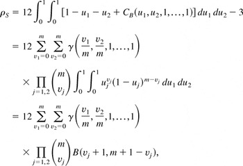
For the BC ρS can be derived as follows:
where γ was defined in (10) and B(a,b)
is the beta function. The first equality follows by writing the BC as
the sum of the product copula and the perturbation term. Notice that
Even when the BC is used as an approximation (see the next section),
the preceding Spearman's rho can be used as an approximation to
the true Spearman's rho of any copula. If enough terms of our
proposed Bernstein approximation are included, Spearman's rho can
be easily found to any degree of accuracy without the need for
evaluating complicated integrals.
We derive the moment generating function (m.g.f.)of the density in
(12). We do it for the one variable case, and then we just extend it to
the k-dimensional case.
where β(v/m) is given by (13) for
k = 1. Before proceeding any further, we notice the following
(see Marichev, 1983, p. 87):
Re c > Re a > 0, where
1F1(a;c; z)
is Kummer's confluent hypergeometric function and
Γ(c) is the gamma function. For a ≡
v + 1, c ≡ m + 2, and z
≡ t this implies
Therefore,
To obtain the m.g.f. for the k-dimensional BC density, we
replace the univariate result in the multivariate definition. Defining
Mc(t) as the m.g.f. of (12), for
t a k × 1 vector,
where [bull ] is the inner product. These results can be used to
further investigate the properties of the BC and its approximations.
Deriving results for the joint moments of the BC is quite easy in
virtue of its incomplete beta function representation. The joint
moments are important for studying the scale-free dependence properties
of the variables.
3. ABC: BERNSTEIN REPRESENTATION OF
ARBITRARY COPULAE
Although the BC should be regarded as a copula in its own right, it
is particularly suited to problems where a parametric copula is
available but in a very complicated form. In this case, the BC can be
used in place of the original copula. As mentioned in Section 1, we
call this the approximate Bernstein copula (ABC) representation. By the
approximation properties of Bernstein polynomials, the coefficients are
simple to find. One may object that Bernstein polynomials have a slower
rate of convergence as compared to other polynomial approximations (see
Theorem 2, which follows). However, they have the best rate of
convergence within the class of all operators with the same shape
preserving property (see Berens and DeVore,
1980).
To give an example of the viability of the Bernstein approximation
and its range of dependence we approximate the Kimeldorf and Sampson
(KS) copula (see, e.g., Joe, 1997, p. 141),
which is equal to
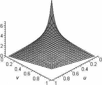
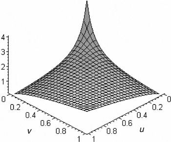
Notice that this copula has unbounded density. Figure 1 shows the three-dimensional graph of the
KS copula density.
KS copula density, θ = 1.06.
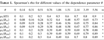
In Table 1, we report the values of
Spearman's rho as a function of the dependence parameter θ in
the approximation for m = 10, 30, 50, 100, 200, 300, and the
corresponding values for the KS copula. Because of computational
difficulties we do not calculate the approximation when the dependence
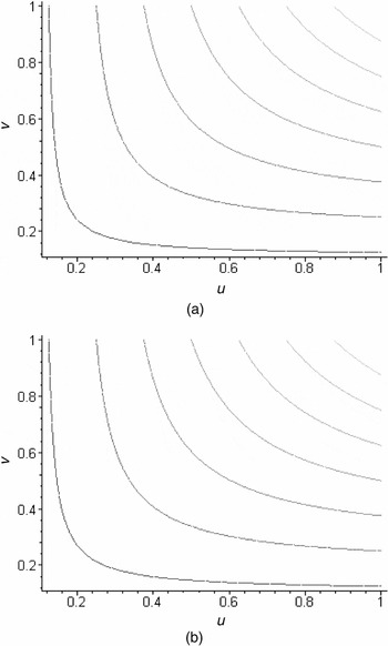
parameter achieves its limiting value (∞). Figure 2 shows the contour plot of the two copulas
when θ = 1.06 and m = 30. These seem to be
indistinguishable.
Spearman's rho for different values of the dependence parameter
θ
(a) KS copula density, θ = 1.06. (b) ABC for the KS copula
(θ = 1.06, m = 30).
All differences are due to polynomials being fairly slow in adjusting
at turning points. Improvements can be achieved by increasing the order
of the polynomial, keeping all computations manageable and
straightforward. Integral evaluation for the computation of
Spearman's rho for the KS copula can only be done numerically.
To lend some rigor to this numerical example, we state the following
theorem.
THEOREM 2. Let f ∈
C[0,1]k and
∂f/∂xj be
Lipschitz ∀j; then
where Bmk is the
k-dimensional Bernstein operator and M is a constant.
Proof. See the Appendix. █
This rate of approximation can be improved using linear combinations
of Bernstein polynomials (see Butzer, 1953).
Let f(2l) (i.e., the 2l
derivative of f) be Lipschitz of order γ; then Butzer
(1953) shows that one can construct a linear
combination of one-dimensional Bernstein polynomials of order
m such that the error is
O(m−l−γ) compared
with O(n−2l−γ)
for the best approximating polynomials of order m (Jackson,
1930, p. 18). However, the coefficients of
Bernstein polynomials have clear interpretations in the case of both
the copula and the copula density. Further, all the derivatives of
Bernstein polynomials converge to the true derivatives of the
approximated function when the latter is differentiable. Other optimal
properties of Bernstein polynomials in connection with the copula
function and joint continuity of Markov operators are discussed in Li,
Mikusiński, and Taylor (1998) and
Kulpa (1999).
A limitation of the BC is that it cannot be used to model extreme
tail behavior defined in terms of the coefficient of tail
dependence.1
Lower and upper tail dependence
are, respectively, defined as
where λL and λU are
between zero and one. No tail dependence corresponds to these
probabilities being exactly zero.
This happens because convergence
under the sup norm is not sufficient for ensuring that the BC and its
approximand converge to an arbitrary limit at the same speed. Nevertheless,
the BC can capture increasing dependence as we move to the tails. In fact, the
KS copula in (14) exhibits lower tail dependence, and the BC can approximate
arbitrarily well the tail behavior of this copula inside the cube.
4. EMPIRICAL BERNSTEIN COPULA: AN
ESTIMATION PROCEDURE
There are several possible estimation procedures that can be employed
to make the BC operational. However, the BC might also be used as an
estimator for unknown copulas. In this case, we would use the BC
density as an estimator, where the coefficients of the copula are given
by the empirical copula and the order of polynomial would be related to
the smoothing properties of the estimator. As mentioned in Section 1,
we call this the empirical Bernstein copula (EBC) density.
4.1. The Empirical Bernstein Copula Density
Let Cn(v1
/m,…,vk
/m) be the empirical copula at (v1
/m,…,vk
/m), i.e.,
where
is the indicator of the set
and tvj
≡ vj /m. By
construction, the empirical copula is a valid distribution function.
However, it has marginals that are uniform only asymptotically;
i.e.,
for j = 1,…,k. Therefore it is a valid
copula only asymptotically.
2 Clearly we could
easily impose the boundary condition
However, this will not ensure that Cn is
monotonically increasing in a finite sample.
The EBC, say,
,
is defined as the usual BC where
Differentiating, it is easy to see that the coefficients of the
polynomial are equivalent to a k-dimensional histogram
estimator (for details of the histogram estimator, see Scott, 1992),
where we use
to stress
that it is a particular estimator and
[utri ]1,…,k is the k-dimensional
difference operator; i.e.,
The optimal choice of m depends on the topology we use. We
choose m to minimize the mean square error (MSE) of the
density; i.e.,
where
∥…∥2 is the L2 norm under
the true probability measure and c is the true copula density.
Just increasing m will reduce the bias but increase the
variance of
.
4.2. Consistency in Mean Square Error of the Estimated
Bernstein Copula Density
We want to choose (16) such that it is optimal under the
L2 norm. The asymptotic properties of this
estimator under the L2 norm have been studied in
detail in Sancetta (2003) under the following
condition.
Condition 1.
u1,…,un is a
sequence of independent strictly stationary uniform
[0,1]k random vectors with copula
C(u) and copula density c(u) that
has finite first derivatives everywhere in the k-cube.
Remark. The independence condition is not required, but we use it to
shorten the proof as much as possible. From the proof of Theorem 3 it can
be seen that the results are still valid under appropriate mixing conditions
by use of known coupling results.
We use [lsim ] to indicate greater or equal up to a multiplicative
absolute constant; e.g., a [lsim ] b implies
∃C, 0 < C < ∞, such that a
≤ Cb. (This notation is commonly used in the empirical
process literature; see, e.g., van der Vaart and
Wellner, 2000.)
THEOREM 3. Let
be the
k-dimensional BC density. Under Condition 1,
The proof of Theorem 3 is given in the next section. The weak limit
implies that convergence is uniform: if a class of functions is
Donsker, then it is Glivenko–Cantelli; i.e., convergence holds
uniformly over the class (see, e.g., van der Vaart and
Wellner, 2000, p. 82). Therefore, the results of Theorem 3 hold
uniformly.
For comparison purposes, let h ≡
m−1 be the smoothing factor in the usual
sense. The bias is of the same order as the bias for the histogram
estimator. In this respect, kernel smoothers would lead to a bias not
higher than O(m−2), as opposed to
O(m−1) in our case. Notice that it
is not possible to reduce the bias to
O(m−2) by shifting the histogram,
i.e., using frequency polygons (for details on frequency polygons, see,
e.g., Scott, 1992, Ch. 4). In this case the
first term in the expansion would vanish, but other terms of the same
order would not. Further, the O(k/m)
rate of approximation of k-dimensional Bernstein polynomials
imposes a lower bound on the bias unless linear combinations of
Bernstein polynomials are used (see the discussion at the end of
Section 3).
Although the bias is of the same order as the histogram estimator,
the variance is of smaller order (except at the edges of the
hypercube):
instead of
O(mk) as is the case for the
histogram and kernel estimators. On the other hand, for
uj = 0,1, for all j's, the
variance is of the same order as for common nonparametric estimators.
The case uj = 0,1 for only some j
is not included because the result is just a mixture of the two extreme
cases: the variance goes down by a factor that is
O(m1/2) for all the coordinates inside
the k-hypercube, whereas for the coordinates on the boundaries
the contribution to the variance is O(m).
As m and n go to infinity, it follows that this
estimator has a rate of consistency
mk/2/n → 0 inside
the hypercube versus mk/n
→ 0 for other common nonparametric estimators, e.g., the Gaussian
kernel. Inside the hypercube, the optimal order of smoothing is
m = O(n2/(k+4)) in
MSE sense versus m =
O(n1/(k+2)) for the histogram
and m = O(n1/(k+4))
for a first-order kernel.
This implies that the Bernstein polynomials require very little
smoothing (i.e., a large order of polynomial, which implies a less
smooth graph). This is due to the fact that Bernstein polynomials are
fairly slow to adjust, as already mentioned in Section 3.
4.3. Simulation
In this section, we use some short simulations to investigate the
finite sample properties of the EBC density. We choose the KS copula in
(14) as the true one. In particular, we let θ = 0.6. This
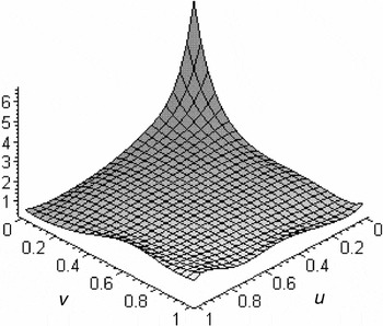
corresponds to ρS = 0.34. Figure 3 shows the plot for the copula density of
the KS copula with dependence parameter θ = 0.6. The KS copula is
singular at the origin. As a condition in Theorem 3 we used the fact
that the copula density is nonsingular. Therefore, comparing this
copula density with the EBC will be of interest for several reasons.
KS copula density, θ = 0.6.
We notice that this copula density exhibits lower tail dependence.
This means specifically that random variables become more dependent on
the left side of their support. This appears to be an important
property when modeling joint financial returns: asset returns are more
dependent when they are negative (for the case of daily financial
returns, see Silvapulle and Granger, 2001;
Fortin and Kuzmics, 2002). By the properties
of the copula function we are not concerned with the marginal
distributions: these either could be known or could be estimated using
a parametric specification or the empirical distribution function.
Assuming the marginals are correctly specified, then, by definition,
the copula is the joint distribution of uniform
[0,1]k marginals. For example, if we were
to model daily financial returns parametrically, the modified Weibull
distribution or the double gamma could be a good choice (e.g., Knight et al., 1995; Laherrère and Sornette, 1998). Therefore,
the copula allows us to divide the estimation problem into two steps,
which are independent. In this simulation, we only consider the
performance of our estimator, so that the marginals are uniform. This
corresponds to the case of marginals being known. Carrying out a
simulation of the whole joint distribution (i.e., copula and marginals)
might be of interest also. However, in this case, the error in the
parametric estimation of the marginal would confound the error in the
estimation of the copula. On the other hand, the purpose of this
simulation is to provide a brief direct illustration of the small
sample properties of our estimator and their link to the theoretical
asymptotic results of Theorem 3.
The realism of the simulation needs to be discussed. We have
arbitrary marginals that could reflect skewness and kurtosis and a
copula that has, as mentioned previously, lower tail dependence in line
with current empirical research on financial returns. It is the latter
we are focusing on in our simulation.
We generate 100 samples of n = 500 observations from the KS
copula with θ = 0.6; the value of n corresponds to the
number of our daily observations (for details on simulating data from
multivariate distributions and copulas, see Li,
Scarsini, and Shaked, 1996). We consider estimation of the BC
density for m = 4,6,…,40. This boils down to finding
the histogram estimator with bin width equal to
m−1 and then applying the Bernstein operator
to it. We plot the estimated copula for m = 12 in Figure 4.
To study the global performance of our estimator, we should look at
the integrated mean square error (IMSE); i.e.,
For each m, we use our 100 samples of 500 observations from
the KS copula to compute an approximate bias squared and variance, say,
.
Both
are obtained by evaluating
at
10,000 uniform [0,1]2 pseudorandom points (for
each m, we just use the same points). Therefore, we
approximate the preceding integral by averaging over these 10,000
points; i.e.,
where
{(uj,vj)}j=110000
is our uniform [0,1]2 sample of points where both
the KS copula density and the EBC density are evaluated. We summarize
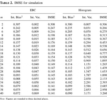
our results in Table 2.3
The results in Table 2 should be
considered purely illustrative. A larger number of Monte Carlo simulations
would be required in order to achieve more accurate convergence.
Unfortunately, our calculations were labor-intensive, and a larger
number of simulations would require more investment in programming to
obtain results within a reasonable time. Another problem is caused by
the use of Monte Carlo integration in place of integration over the
unit square. In this case, more advanced approaches could have been
used, such as quasi-random numbers to bound the error by a quantity
O(ln(n)k/n) (for
k = 2 dimensions in our case) instead of the usual
for the Monte Carlo integration approach (for further details, see, e.g.,
Spanier and Maize, 1994).
We also
report the same results when the copula is estimated using the
two-dimensional histogram estimator. Because the EBC density is
obtained from the histogram, it is natural to make comparisons with the
two-dimensional histogram.
The main result of Table 2 is that applying
the Bernstein operator to the two-dimensional histogram estimator
allows us to decrease the size of the mesh and, consequently the bias,
keeping the uncertainty (i.e., the variance) low. Further, the results
for the ECB do not seem to be particularly sensitive to m as
opposed to the histogram.
The results agree with the asymptotic results in Theorem 3 in the
sense that the variance grows linearly in m as opposed to the
histogram estimator, whose variance appears to be quadratic in
m. The biases also agree with Theorem 3 (the EBC and the
histogram have similar biases), though not as accurately in small
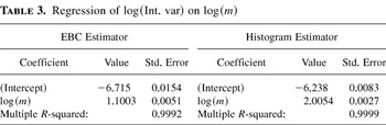
samples. In Table 3 we report the results
from regressing the log of the integrated variance of the two
estimators (the EBC and the histogram) on the log of m. We use
m = 4,5,…,41 with the corresponding estimated variances
(i.e., 38 observations). The slopes of the regression support the
conclusions of Theorem 3. For the sake of conciseness, we do not report
results from the regression of the biases because the coefficients of
log m are similar for the two estimators (as implied by
Theorem 3) but very sensitive to the choice of range of m due
to the influence of higher order terms.
Regression of log(Int. var) on log(m)
4.4. Proof of Theorem 3
The proof of part ii of Theorem 3 is based on the normal
approximation to the binomial distribution (e.g., see Stuart and Ord, 1994, pp. 138–140). In
particular, let
and
Then
A formal proof may be given through the Edgeworth expansion for
z = (v/m − u) to prove
that the error is uniform. Taking squares of the two distributions
(i.e., the binomial and the Gaussian),
where again the error holds uniformly. With this remark, we can prove
Theorem 3.
Notation. We use
u1,…,un to
indicate n copies of k-dimensional uniform random vectors in
[0,1]k. On the other hand u =
(u1,…,uk)
denotes a fixed, but arbitrary, k-dimensional vector.
Following Abadir and Magnus (2000), we define
Di c(u) ≡
(∂c(us)/∂ui)|us=u.
Proof of Theorem 3.
,
which we can rewrite as
Clearly,
where the second inequality follows from the same argument as in the
previous proof. Because the Bernstein operator is bounded, by
Fubini's theorem, it is sufficient to consider
i.e., the bias for a histogram estimator. Therefore (e.g., Scott,
1992, p. 81; or just use (22), which follows,
where no Taylor expansion is required),
Therefore,
For the variance, notice that the probability of one observation
falling inside a subset of the hypercube is equal to the probability of
a success in a Bernoulli trial. We know that the probability of
n successes, where n is the sample size, is given by
a binomial distribution. By the variance of n independent
Bernoulli trials
where
Consider the following simple identity for any differentiable
function f:
where the left-hand side can be recovered by simple integration of
the second term on the right-hand side. By direct application of (20)
we have
Now, by Condition 1, D1
c(u1s,u2s,…,uks)
≤ M for some M < ∞. Therefore, the last
term in (21) is bounded by
Substituting in (21),
Applying (20) repeatedly, we have
Because
ps,v1···vk
≤ 1, it follows that
(ps,v1···vk)2
=
o(ps,v1···vk).
Therefore, substituting (22) in (19), we have that
We use (18) to approximate (23). By Condition 1,
c(tv1,…,tvk)
is bounded, say, by M < ∞. Recall that
tvj ≡
vj /m, j =
1,…,k. Consequently, solve the following type of
integral:
Simply make the following change of variable,
,
with Jacobian
.
Then
Therefore, Γj =
O(m−1/2). This shows that
integration leads to a drop in asymptotic magnitude equal to
m−1/2 for each dimension. Let
λj ≡
[uj(1 −
uj)]1/2; then
At the edges of the hypercube, i.e., u = 0,1,
(Pvj,m−1(u))2
=
Pvj,m−1(u);
then
The MSE convergence simply follows by considering the leading terms
for the square bias and the variance for the two distinct cases:
.
The optimal order of
the polynomial follows by minimization of asymptotic MSE with respect
to m. Inside the hypercube we have
which implies m(k+4)/2 =
O(n). Similarly, for the density at the boundaries of
the k-cube,
which implies mk+2 =
O(n).
The finite-dimensional distributions of the EBC density converge to a
normal distribution. This follows from the fact that it is the sum of
bounded random variables and Condition 1 (weaker conditions than i.i.d.
are clearly sufficient for the central limit theorem). But the BC
density has m − 1 bounded derivatives (recall that
Bernstein polynomials are closed under differentiation), and any
Bernstein polynomial is Lipschitz. By Theorem 2.7.1 in van der Vaart
and Wellner (2000, p. 155) the class of functions
that satisfy the properties just mentioned has finite ε bracketing
numbers of order
exp{ε−(k/(m−1))}. It
follows that their entropy integral with bracketing is finite. This is
enough to show (for the i.i.d. case, see Ossiander,
1987; for generalizations, see Pollard,
2001) that the BC density converges to a Gaussian process with
continuous sample paths. The
term is required for the leading term in the variance expansion to be
independent of n; i.e., m → ∞ as
n → ∞ (as usual for nonparametric estimators). The
same condition applies to the copula because it is m times
differentiable together with the same properties of the density.
Clearly, the simple root-n standardization is employed in this case
(integration absorbs the smoothing parameter). █
From the proof it is clear that what drives the variance down is the
fact that approximating the square of
Pv,m−1(u) leads to
a normal approximation times an extra term that is
O(m−1/2). To provide more
intuition on this result and the difference between the edges of the
box and the points inside it, we provide the following heuristic
explanation. Bernstein polynomials average the information about the
function throughout its support; recall the singular integral
representation in (4). On the other hand, the result at the corners of
the hypercube is clear: the approximation at these points is exact, and
it is not influenced by the behavior of the function in its domain;
i.e., it is exactly local so that we just recover the properties of the
histogram estimator.
5. CONCLUSION AND SOME FURTHER EXTENSIONS
We studied a new object in multivariate analysis called the Bernstein
copula (BC). Furthermore, we showed that, subject to regularity, any
copula can be represented (approximated) by some BC. This copula
representation should allow us to take advantage of the properties of
the copula function whenever multivariate normality is not a good
assumption.
We made the procedure operational by providing an empirical
estimation procedure with its rates of consistency and an interesting
result for the variance. The result for the variance may provide a
partial solution to the curse of dimensionality, particularly in
semiparametric estimation, i.e., when the marginals are known.
The study of the BC led us to consider many topics all at once. It is
clear that much has been omitted from this paper. We did not discuss
joint continuity of the BC under the *-product defined by Darsow et al.
(1992) (see Kulpa,
1999; Li et al., 1998). The *-product
is a powerful tool that allows us to define Markov processes and
general time series dependence concepts. The BC is closed under this
operation.
The consistency results for the EBC have been derived under the
condition of i.i.d. observations. Although the more general case of
stationary random variables could be dealt with (under suitable mixing
conditions), for the sake of conciseness we refrained from doing so. We
restricted m to be the same for all coordinates. This is not
necessary, but the notation would have been cumbersome. What seems more
relevant in practice is the actual choice of m (possibly
different in each coordinate) in empirical work. We did not discuss
this issue because it is a common problem for similar (nonparametric)
estimators to the EBC. As shown in our example, one may consider some
metric and minimize it in terms of m. The results in Table 2 show that the error is not particularly
sensitive to the choice of m as opposed to the histogram
estimator. In practice we may use cross validation or some modified
version of it (the true estimator would be approximated using the
jackknife). For more details on this and related limitations of this
approach, the reader is referred to Scott (1992). We could have compared our estimator with
the Genest and Rivest (1993) nonparametric
procedure for selecting the best bivariate archimedean copulas (e.g.,
for details on archimedean copulas, see Joe, 1997, p. 86). These authors derive an estimator,
say, Kn(v), for a function
K(v), which is closely related to the generator of an
archimedean copula. Therefore, their approach could be used to estimate
empirically the generator of a bivariate archimedean copula and from
that to obtain an estimator for a bivariate archimedean copula.
However, using the words of these authors: their approach “often
proves more convenient in application to use … as a tool for
identifying the parametric family of Archimedean copulas that provides
the best possible fit to the data”; further, “one may be
tempted to determine directly from
Kn(v) the Archimedean
copula” (p. 1035). “Though this would be formally possible,
whenever v −
Kn(v−) < 0
for all 0 < v < 1, it generally will be theoretically
more meaningful—as well as computationally more
convenient—to use Kn as a tool to
help identify the parametric family of Archimedean copulas that
provides the best possible fit to the data” (p. 1038). Indeed, we
experienced computational difficulties estimating empirically an
archimedean copula using this approach. Although the KS copula used in
our simulation as the true model belongs to the class of bivariate
archimedean copulas, our estimator is not restricted to this class, has
wider application, and is easier to compute.
Finally, alternative estimation procedures have not been considered
in detail. Although the paper provides a promising result for the
variance of the empirical estimator, this is one among many others that
could be studied. For example, one could look at the following
estimation problems:
where Pn is the empirical measure,
Cn is the empirical copula,
λn is a smoothing parameter going to zero as
n → ∞, the unqualified integral is a Lebesgue
integral,
is the differential operator of
order α, i.e.,
.
However, unlike the case of the EBC density, these estimators will not
automatically lead to a copula unless constraints are imposed.
Nevertheless, under suitable constraints, it seems plausible that the
study of these estimators may lead to analogous results in virtue of
the kernel representation of the BC. Some of the issues omitted from
this paper are the subject of current research.
APPENDIX: PROOFS
Proof of Theorem 1. Consider the BC
CB(u1,…,uk)
as an approximation to a copula
C(u1,…,uk),
i.e.,
Then (5) and (6) are sufficient for C(v1
/m,…,vk
/m) to be a copula. Because Bernstein polynomials do not
interpolate exactly, (5) and (6) are not necessary for
CB(u1,…,uk)
to be a copula. █
Proof of Theorem 2.
∇f ≡
[f′1(s1,…,sk),…,f′k(s1,…,sk)],
where
f′j(s1,…,sk)
≡ ∂f
(s1,…,sk)/∂sj
and r is a vector valued function that defines the path
between the end points of the integral. By definition,
∇f is a conservative vector field, and so the path of
integration is irrelevant. The preceding line integral can be split
into k integrals along any paths parallel to the axis and
perpendicular to each other. For example, we can write
Now, considering the jth term,
From here the crude result of the theorem can be obtained assuming
that f′j ∈
LipMj1, i.e.,
f′j satisfies the Lipschitz condition
with constant Mj and exponent 1:
It follows that the last integral in (A.1) does not exceed
.
Therefore,
for any X, where the first term on the right-hand side of
(A.1) is exactly zero when the Bernstein operator is applied to
(vj /mj
− xj). █