


1 INTRODUCTION
Checking the correct specification of a model is empirically relevant, as a misspecified model can yield inconsistent estimates and provide a misleading counterfactual analysis. In this article, we contribute to the literature by providing a specification test for semiparametric models with nonparametrically generated regressors. Such regressors are not observed by the researcher but are nonparametrically identified and estimable. Examples of semiparametric models with generated variables are common in empirical frameworks. They include endogenous regressors models with control functions (Newey, Powell, and Vella, Reference Newey, Powell and Vella1999; Blundell and Powell, Reference Blundell and Powell2004), semiparametric sample selection models, extension of tobit models (Escanciano, Jacho-Chávez, and Lewbel, Reference Escanciano, Jacho-Chávez and Lewbel2016), or semiparametric empirical games with incomplete information (Aradillas-Lopez, Reference Aradillas-Lopez2012; Lewbel and Tang, Reference Lewbel and Tang2015).
Let
$Y\in \mathbb R $
 ,
$Z\in \mathbb R ^p$
 , and
$X\in \mathbb R^{p_X} $
 . Our goal is to test the null hypothesis

for some real vector
$\beta _0\in B$
 and a nonparametric function
$G_0$
 , against its logical complement
$\mathcal H _1$
 , where
$q:B\times \mathbb {R}^{p_X+1}\mapsto \mathbb {R}^d$
 is a known vector-valued function, B is a finite-dimensional parameter space, and

is a nonparametric function, with
$D\in \mathbb {R}$
 . The null hypothesis is featured by the presence of the generated variable
$H(Z)$
 . This means that
$H(Z)$
 is latent, but it is identified and estimable in the first-step nonparametric regression (2). The conditional moment restriction in (1) arises from the above-mentioned empirical models, see Section 4 for details. In typical applications
$d<p_X+1$
 , although we do not require this condition to hold.
Our main contributions are twofold. First, we develop a test for the null hypothesis in (1) featured by the presence of generated variables. Due to the presence of generated variables, the null hypothesis in (1) cannot be tested using existing methods. Our test statistic is based on bias-corrected nonparametric estimators, so their tuning parameters do not require undersmoothing. Second, we construct and show the validity of a novel wild bootstrap procedure to compute the critical values. Our wild bootstrap procedure (i) uses the information under the null hypothesis and (ii) unlike existing procedures for inference in the presence of generated variables, does not require estimating nonparametric derivatives.
Our first main contribution is thus to propose a test for the conditional moment restriction in (1). If this moment condition did not contain the generated variable
$H(Z)$
 , a specification test could be based on procedures already available in the literature for models where all regressors are observed (see, e.g., Delgado and Manteiga, Reference Delgado and Manteiga2001; Xia et al., Reference Xia, Li, Tong and Zhang2004). However, since the generated variable
$H(Z)$
 is not observed, these tests cannot be implemented in the setting considered here.
To construct our test statistic, we proceed in three steps: in a first step we estimate the generated variable
$H(Z)$
 , in a second step we estimate the parameter
$\beta _0$
 , and in a third step we estimate the nonparametric function
$G_0$
 . This allows us to compute the residuals of the semiparametric model. Our test statistic is then based on an empirical process involving the estimated residuals, see Section 2 for details. A specific feature of this setting is that replacing the generated regressor
$H(Z)$
 with its estimate in the first step introduces an estimation error that affects the asymptotic behavior of our test statistic. Hence, it needs to be taken into account.
A distinguishing feature of our test is the presence of bias corrections for the nonparametric estimators of the first and third steps. We show that, in our setting, these bias corrections guarantee a small bias property of our test statistic. This means that the bias of our test statistic converges to zero faster than the bias of the nonparametric estimators on which it is based (see also Newey, Hsieh, and Robins, Reference Newey, Hsieh and Robins2004). Such a feature allows us to avoid using undersmoothed tuning parameters for the nonparametric estimators of the first and third steps. To the best of our knowledge, this is a novel approach in semiparametric models with generated variables.
Our second main contribution is to construct a novel wild bootstrap procedure to compute valid critical values for our test. We show that asymptotically our statistic converges to an intricate distribution depending on unknown features of the data-generating process (DGP). Therefore, the asymptotic distribution cannot be directly employed to obtain the critical values. This problem also arises in the semiparametric specification tests of, for example, Delgado and Manteiga (Reference Delgado and Manteiga2001) and Xia et al. (Reference Xia, Li, Tong and Zhang2004) who develop bootstrap procedures to obtain the critical values. However, their bootstrap procedures are not valid in our context due to the presence of generated regressors: since their bootstrap procedures are developed for settings without generated variables, they cannot replicate the estimation error arising from the generated regressors.
Other procedures are developed in the literature to adjust testing methods for the presence of generated variables (see Wooldridge, Reference Wooldridge2010, Chap. 6; Hahn and Ridder, Reference Hahn and Ridder2013; Hahn, Liao, and Ridder, Reference Hahn, Liao and Ridder2018). Such procedures consist of estimating the adjustment terms due to the generated variables in the influence function representation (IFR) of the statistic, and then correcting the standard errors of the test. Using this approach in our testing problem would be difficult, as the adjustment terms in our context involve nonparametric derivatives. Since nonparametric derivatives are hard to estimate, such an approach would not be practically appealing.
Thus, in this article, we construct a novel wild bootstrap procedure for obtaining valid critical values. In particular, our contribution is to develop a wild bootstrap method that does not require estimating nonparametric derivatives and can replicate the estimation error coming from the generated variables. To the best of our knowledge, this is a novel contribution in the literature on generated regressors. The bootstrap we develop here imposes the null hypothesis when resampling the observations. This feature is attractive, as it means that we are using all the information available when constructing the critical values for testing. We develop the wild bootstrap test so that also the bootstrapped statistic has a small bias property, as well as the sample statistic.
1.1 Related Literature
Beyond the studies already cited, there is a large literature analyzing the problem of estimation with generated variables. Early work includes Pagan (Reference Pagan1984). More recent results are presented in Rothe (Reference Rothe2009), Sperlich (Reference Sperlich2009), Mammen, Rothe, and Schienle (Reference Mammen, Rothe and Schienle2012), Gutknecht (Reference Gutknecht2016), Mammen, Rothe, and Schienle (Reference Mammen, Rothe and Schienle2016), and Bravo, Escanciano, and Van Keilegom (Reference Bravo, Escanciano and Van Keilegom2020). Within a semiparametric context, Hahn and Ridder (Reference Hahn and Ridder2013) analyze the impact of generated regressors on the asymptotic distribution of a finite-dimensional estimator. Escanciano, Jacho-Chávez, and Lewbel (Reference Escanciano, Jacho-Chávez and Lewbel2014) obtain an expansion of the residuals from a regression involving variables estimated in a preliminary step. These papers focus on estimation and do not address specification testing in the presence of generated regressors.
From a statistical point of view, our work is related to Escanciano et al. (Reference Escanciano, Jacho-Chávez and Lewbel2014) with two important distinctions. First, in this article, we develop a wild bootstrap test, while Escanciano et al. (Reference Escanciano, Jacho-Chávez and Lewbel2014) are not concerned with constructing a bootstrap procedure. Second, the residuals entering our statistic involve bias correction terms which are not present in their context. This allows us to avoid undersmoothing and to obtain a small bias property of our statistic.
Finally, our work is related to the extensive literature on specification testing in semiparametric models (see, e.g., Bierens, Reference Bierens1982). The distinctive feature of our work is the presence of generated variables that introduce extra terms in the asymptotic expansion of our statistic.
1.2 Organization of the Article
Section 2 constructs the test statistic, sets up the assumptions, and obtains the asymptotic behavior of our statistic. Section 3 details the construction of our wild bootstrap procedure and shows its validity for computing the critical values. The main applications of our test are presented in Section 4. Section 5 describes the practical implementation of our test, provides evidence about its finite-sample performance, and finally shows its application to a real data set. The Appendix contains the proofs of the main results, additional technical lemmas, and an extension to models with semiparametrically generated regressors.
2 THE TEST
For the sake of generality, we test a generalized version of Equation (1), namely,

against its logical complement
$\mathcal {H}_1$
 , where
$\nu :\mathbb {R}^{p_X+1}\mapsto \mathbb {R}^{p_\nu }$
 ,
$q:B\times \mathbb {R}^{p_X+1}\mapsto \mathbb {R}^d$
 ,
$\nu $
 and q are known functions,
$H(Z)$
 is as in Equation (2), and the
$\sigma $
 -field generated by
$q(\beta ,X,H(Z))$
 is contained in the
$\sigma $
 -field generated by
$\nu (X,H(Z))$
 for all
$\beta \in B$
 .Footnote
1
Note that Equation (3) encompasses (1) as a special case.Footnote
2
To use a more compact notation, we define

Let us assume that
$W(\beta )$
 is continuously distributed for any
$\beta \in B$
 , and let
$f_{W(\beta )}$
 be the density function of
$W(\beta )$
 with respect to the Lebesgue measure. Since the
$\sigma $
 -field generated by
$W(\beta _0)$
 is a subset of the
$\sigma $
 -field generated by
$\nu (X,H(Z))$
 , the null hypothesis in (3) is equivalent to

for some
$\beta _0\in B$
 . We have introduced the density function
$f_{W(\beta _0)}$
 to avoid a random denominator in the estimation of
$G_{\beta _0}$
 (see Section 2.1 for details). Equation (5) is a conditional moment restriction. To test such an equation, we consider an equivalent continuum of unconditional moments. Let us assume that
$[Y-G_{\beta _0}(W(\beta _0))] \, f_{W(\beta _0)}(W(\beta _0))$
 has finite second moments and that
$\nu (X,H(Z))$
 is a bounded random variable.Footnote
3
Then, by Bierens (Reference Bierens2017, Thm. 2.2), the null hypothesis in (5) is equivalent to

and for some
$\beta _0\in B$
 , where
$\mathcal S$
 is a set containing a neighborhood of the origin,
$\varphi _s(X,H(Z)):=\varphi (s^T \nu (X,H(Z)))$
 , and
$\varphi $
 is an analytic non-polynomial function with
$\partial ^{l}\varphi (0)\neq 0$
 for all
$l\in \mathbb {N}$
 . Examples of
$\varphi $
 include
$\exp (\cdot )$
 ,
$\cos (\cdot )+\sin (\cdot )$
 , and
$\exp (\sqrt {-1}\cdot )$
 (see Bierens, Reference Bierens2017). Now, the formulation of the null hypothesis into a continuum of unconditional moments is quite convenient, as it allows us to construct a test without estimating
$\mathbb E \{Y|\nu (X,H(Z))\}$
 . Differently, constructing a test based on the conditional moments in (5) or (3) would require estimating
$\mathbb E \{Y|\nu (X,H(Z))\}$
 . From a practical point of view, this would complicate the implementation of the test, as we should select additional smoothing parameters, say bandwidths.
Suppose we observe an independent and identically distributed (i.i.d.) sample
$\{Y_i,X_i,Z_i,D_i\}_{i=1}^n$
 from
$(Y,X,Z,D)$
 . Let us denote by
$\mathbb P_n$
 the empirical mean operator, that is,
$\mathbb P_n g(Y,X,Z,D)=n^{-1}\sum _{i=1}^n g(Y_i,X_i,Z_i,D_i)$
 for any function g. Also, let
$\mu $
 be a finite measure supported on
$\mathcal S$
 and let
$\beta _0=\arg \min _{\beta \in B}\mathbb {E}[Y-G_{\beta }(W(\beta ))]^2$
 be the pseudo-true value of the finite-dimensional parameter.Footnote
4
Note that the null hypothesis in (6) is equivalent to

Thus, if we knew
$ G_\beta(W(\beta))$
 ,
$f_{W(\beta)}(W(\beta))$
 , and
$\beta _0$
 , we could test (6) using the Cramér–von Mises functional

However, such an “oracle” statistic cannot be used in practice, as
$G_{\beta }$
 ,
$f_{W(\beta )}$
 , and
$\beta _0$
 are unknown and must be estimated. Now, if we could observe the generated regressor
$H(Z)$
 , a test for (6) could be constructed in two steps. In the first step, we could estimate
$\beta _0$
 by, say,
$\widehat \beta $
 . In the second step, given
$W(\widehat \beta )=q(\widehat \beta ,X,H (Z))$
 , we could regress nonparametrically Y on
$W(\widehat \beta )$
 to get an estimate of
$G_{\beta _0}$
 , and we could construct a nonparametric density estimator of
$f_{W(\beta _0)}$
 based on
$W(\widehat \beta )$
 . Then, a statistic as in (7) based on such estimators could be used for testing (6). A test of this type is proposed in Xia et al. (Reference Xia, Li, Tong and Zhang2004) and Delgado and Manteiga (Reference Delgado and Manteiga2001) who develop bootstrap tests for equations similar to (6) when all regressors are observed. However, since the generated variable
$H(Z)$
 is not observed, such tests cannot be implemented in our context.
Due to the presence of the generated variable
$H(Z)$
 , we compute a feasible test statistic by a three-step estimation. In the first step, based on (2), we regress nonparametrically D on Z to get an estimate of H, say
$\widetilde H$
 . In the second step, we obtain an estimator of
$\beta _0$
 , say
$\widehat \beta $
 . Finally, in the third step, given
$\widetilde W(\widehat \beta ):=q(\widehat \beta , X, \widetilde H (Z))$
 , we regress nonparametrically Y on
$\widetilde W(\widehat \beta )$
 to get an estimate of
$G_{\beta _0}$
 , and we construct a nonparametric density estimator of
$f_{W(\beta _0)}$
 based on
$\widetilde W (\widehat \beta )$
 . Plugging these estimators into (7) gives a feasible test statistic. In the next section, we detail such a three-step estimation procedure.
2.1 The Test Statistic
2.1.1 First-Step Estimation
Let
$K_H$
 be a kernel on
$\mathbb {R}^p$
 and
$h_H$
 be a bandwidth. We define

The estimation of the generated variable
$H(Z)$
 could be based on
$\widehat {H}(z):=\widehat {T}^{D}_Z(z)/\widehat {f}_Z(z)$
 . However, a test based on the first-step estimator
$\widehat H$
 would necessitate some undersmoothing, see Section 2.2 for details. This would complicate the implementation of the test, as it would make tricky the choice of the first-step bandwidth. Newey et al. (Reference Newey, Hsieh and Robins2004) develop an approach based on twicing kernels to avoid undersmoothing and achieve a small bias property in the context of semiparametric estimators when all regressors are observed. Here, to avoid undersmoothing and obtain a small bias property of our test statistic, we instead use an
$L_2$
 boosted or, equivalently, a bias-corrected estimator in the first step. These types of estimators have been introduced in Di Marzio and Taylor (Reference Di Marzio and Taylor2008) and Park, Lee, and Ha (Reference Park, Lee and Ha2009) for kernel smoothing estimation. Xia et al. (Reference Xia, Li, Tong and Zhang2004) and Lapenta and Lavergne (Reference Lapenta and Lavergne2025) used similar bias corrections for tests when all regressors are observed. The procedure works as follows. Given the initial estimator
$\widehat H$
 , we compute the residuals
$D_i-\widehat H (Z_i)$
 for
$i=1,\ldots ,n$
 . Then, we construct a kernel estimator
$\widehat {T}^{D-\widehat H}_Z(z)/\widehat f_Z (z)$
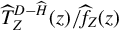 , where
$\widehat {T}^{D-\widehat H}_Z$
 is defined similarly as in (8), with the difference that the projected variable is
$D-\widehat {H}(Z)$
 instead of D. Here,
$-\widehat {T}^{D-\widehat H}_Z(z)/\widehat f_Z (z)$
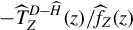 is an estimate of the bias of
$\widehat H(z)$
 (see Xia et al., Reference Xia, Li, Tong and Zhang2004). Finally, we consider the updated or bias-corrected estimator
$\widehat H + \widehat {T}^{D-\widehat H}_Z/\widehat f_Z $
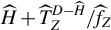 . Such a procedure can be iterated a finite number of times, as proposed in Di Marzio and Taylor (Reference Di Marzio and Taylor2008) and Park et al. (Reference Park, Lee and Ha2009). Here, we restrict ourselves to a one-step boosting: this is enough for our purpose to avoid undersmoothing and guarantee a small bias property of the test statistic.
To precisely define the estimator, let us denote with
$\mathbb I \{\mathcal {A}\}$
 the indicator function of the event
$\mathcal {A}$
 , and let us assume that
$(X,Z)$
 admits a joint density f with respect to the Lebesgue measure. We define

where
$(\tau _n)_n$
 is a sequence of positive numbers converging to zero, whose features are specified in Section 2.2. Indeed,
$K_0$
 and
$h_0$
 denote a kernel and a bandwidth, while
$\widehat f$
 is the kernel estimator of the joint density of
$(X,Z)$
 . We introduce the trimming factor
$\widehat t$
 in
$\widehat {T}^{D - \widehat H}_Z$
 to control for the random denominator of
$\widehat H$
 and trim the most extreme observations.Footnote
5
Then, we estimate H by

As noted in Xia et al. (Reference Xia, Li, Tong and Zhang2004),
$-\widehat T ^{D-\widehat H}_Z/\widehat f_Z$
 can be interpreted as an estimator of the bias of
$\widehat H$
 . So,
$\widetilde H$
 can be thought of as a bias-corrected estimator. Similar nonparametric bias corrections are studied in Di Marzio and Taylor (Reference Di Marzio and Taylor2008) and Park et al. (Reference Park, Lee and Ha2009) for estimation purposes. In our case, we do not apply these bias corrections for estimation purposes. As we argue in Section 2.2, our motivation for using these bias corrections is to obtain a small bias property of the test statistic and to avoid undersmoothing.
2.1.2 Second-Step Estimation
In the second step, we estimate
$\beta _0$
 on the basis of the estimator of the generated variable
$H(Z)$
 . Let
$\widetilde W_i (\beta ):=q(\beta ,X_i, \widetilde {H}(Z_i))$
 for
$i=1,\ldots ,n$
 , and let us recall that d is the dimension of
$\widetilde W(\beta )$
 . For a kernel K and a bandwidth h, we define

Once again, the trimming factor
$\widehat t$
 is used in the above expressions to control for a random denominator in
$\widetilde W(\beta )$
 , that is, in
$\widetilde H$
 , and trim the most extreme observations. Then, an estimator of
$\mathbb E \{Y|W(\beta )=w\}$
 is

We estimate
$\beta _0$
 by a semiparametric least squares (SLS) principle:

We remark that in the above objective function only the first-step estimator
$\widetilde H$
 is bias corrected, while
$\widehat G _{\widetilde W (\beta )}$
 does not contain bias corrections. As we show in Lemma B.2 in the Supplementary Material, this is enough to obtain a small bias property of our test statistic.
An SLS estimator is also used in the specification test proposed by Xia et al. (Reference Xia, Li, Tong and Zhang2004), where all variables are observed. Unlike Xia et al. (Reference Xia, Li, Tong and Zhang2004), our context is characterized by the generated variable
$H(Z)$
 , so the SLS estimator used in our test is based on the first-step nonparametric estimator
$\widetilde H$
 . This implies that the estimation error from
$\widetilde H$
 will appear in the IFR of
$\widehat \beta $
 (see Lemma B.2 in the Supplementary Material). An SLS estimator for index models with generated variables was also proposed in Escanciano et al. (Reference Escanciano, Jacho-Chávez and Lewbel2016). However, in our case,
$\widehat \beta $
 is based on the bias-corrected estimator
$\widetilde H$
 : this allows us to avoid undersmoothing in the first-step estimation and to obtain a small bias property of the test statistic. Furthermore, Escanciano et al. (Reference Escanciano, Jacho-Chávez and Lewbel2016) do not consider specification testing or bootstrap procedures.
2.1.3 Third-Step Estimation
For
$\widehat \varepsilon _i := Y_i - \widehat {G}_{\widetilde W (\widehat \beta )}(\widetilde W _i (\widehat \beta ))$
 , we let

The role of the trimming
$\widehat t$
 in the above display is to control for a random denominator in
$\widehat G _{\widetilde W (\widehat \beta )}$
 and
$\widetilde W(\widehat \beta )$
 . Similarly to the first-step estimation,
$-\widehat {T}^{\widehat \varepsilon }_{\widetilde W (\widehat \beta )}/\widehat f _{\widetilde W (\widehat \beta )}$
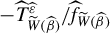 is an estimate of the bias of
$\widehat G _{\widetilde W (\widehat \beta )}$
 . Thus, we define the bias-corrected estimator of
$G_{\beta _0}$
 as

Let us denote the bias-corrected residuals as
$\widetilde \varepsilon _i :=Y_i-\widetilde {G}_{\widetilde W (\widehat \beta )}(\widetilde W_i (\widehat \beta ))$
 , for
$i=1,\ldots ,n$
 . Our feasible statistic is given by

Let us comment on the above expression. The weighting by the estimated density
$\widehat f_{\widetilde W(\widehat \beta )}$
 allows us to get rid of the random denominator in
$\widetilde G _{\widetilde W (\widehat \beta )}$
 . This has a double role. First, it “stabilizes” the behavior of
$S_n$
 by avoiding a denominator that can be close to zero if observations on the “tails” are included in the computation of
$S_n$
 . Second, avoiding a random denominator in
$\widetilde G _{\widetilde W (\widehat \beta )}$
 simplifies our proofs for obtaining the asymptotic behavior of
$S_n$
 . However, due to the presence of generated variables, we still have to control for a random denominator in
$\widetilde W (\widehat \beta )$
 , that is, in
$\widetilde H (Z)$
 . This is the reason why we include the trimming
$\widehat t$
 in the computation of
$S_n$
 so as to trim the most extreme observations. Since
$\widehat t$
 tends to one asymptotically (see Appendix E of the Supplementary Material), the range of values of
$(X,Z)$
 used for the test tends to its support.
The asymptotic behavior of
$S_n$
 is determined by the empirical process
$\sqrt {n} \, \mathbb P _n\, \widetilde \varepsilon \,\,\, \widehat f_{\widetilde W (\widehat \beta )}(\widetilde W (\widehat \beta ))\ \varphi _s(X,\widetilde H (Z))\,\,\widehat t$
 . As mentioned earlier, a Cramér–von Mises statistic similar to
$S_n$
 has already been used for testing equations similar to (6) without generated variables, see Xia et al. (Reference Xia, Li, Tong and Zhang2004) and Delgado and Manteiga (Reference Delgado and Manteiga2001). Differently, our context is featured by the presence of the generated regressors
$H(Z)$
 that are replaced by the first-step estimates
$\widetilde H (Z)$
 . Such a replacement introduces an estimation error that needs to be taken into account. So, when obtaining the IFR of the empirical process underlying
$S_n$
 , we are faced with the challenge of controlling for an estimation error that is not present in Xia et al. (Reference Xia, Li, Tong and Zhang2004) and Delgado and Manteiga (Reference Delgado and Manteiga2001). The estimation error from
$\widetilde H (Z)$
 is non-negligible, since it appears in the IFR of the empirical process underlying
$S_n$
 . See the next section for details.
Beyond the Cramér–von Mises functional in (15), other transformations of the empirical process
$\sqrt {n} \, \mathbb P _n\, \widetilde \varepsilon \ \widehat f_{\widetilde W (\widehat \beta )}(\widetilde W (\widehat \beta ))\ \varphi _s(X,\widetilde H (Z))\,\,\widehat t$
 could be used as test statistics. One of these options is the Kolmogorov–Smirnov functional which takes the following form:

Our results in Sections 2.2 and 3 directly extend to this statistic also. However, throughout this article, we prefer focusing on the Cramér–von Mises statistic
$S_n$
 in (15) for two main reasons. First, as we show in Section 5.1, the Cramér–von Mises statistic in (15) has a simple closed-form expression that can be easily computed. Differently, the Kolmogorov–Smirnov statistic in (16) does not have a closed-form expression. Second, the Kolmogorov–Smirnov statistic requires a numerical maximization that is computationally costly.
2.2 Assumptions and Asymptotic Behavior of the Test Statistic
Let us start by introducing some definitions. We define the differential operator

Definition 2.1. (a)
$\mathcal {G}_\lambda (\mathcal {A}) = \left \{g:\mathcal {A}\mapsto \mathbb {R} : \sup _{a\in \mathcal {A}}|\partial ^l g(a)|< M \text { for all } |l|\leq \lambda \right \}$
 , where M is a fixed constant.Footnote
6
(b)
$\mathcal {K}_{\lambda }^{r}(\mathbb R ^d)\ :=\{(u_1,\ldots ,u_d)\mapsto \prod _{j=1}^d k(u_j)$
 : k is a univariate kernel of order r,
$\lambda $
 times continuously differentiable with uniformly bounded derivatives, symmetric about zero, and with bounded support
$\}$
 .
We next introduce the assumptions and then we comment on them.
Assumption A. (i)
$\{Y_i, X_i, Z_i, D_i\}_{i = 1}^n$
 is an i.i.d. sample of bounded random variables defined on the probability space
$(\Omega ,\mathcal {O},P)$
 . (ii)
$\mathbb {E}\{Y|X,Z\}=\mathbb {E}\{Y|\nu (X,H(Z))\}$
 . (iii) The
$\sigma $
 -field generated by
$\nu (X,H(Z))$
 contains the
$\sigma $
 -field generated by
$W(\beta )$
 for every
$\beta \in B$
 . (iv)
$\mathcal S \subset \mathbb {R}^{p_\nu }$
 is a compact set containing a neighborhood of the origin. (v)
$\varphi _s(x,H(z))=\varphi (s^T\,\nu (x,H(z)))$
 with
$s\in \mathcal {S}$
 and
$\varphi $
 analytic non-polynomial function such that
$\partial ^l \varphi (0)\neq 0$
 for all
$l\in \mathbb {N}$
 .
Let us recall that
$G_\beta (w)=\mathbb {E}\{Y|W(\beta )=w\}$
 with
$W(\beta )=q(\beta ,X,H(Z))$
 . We denote by
$\partial _{\beta _j}$
 the differential operator with respect to the jth component of
$\beta $
 and let
$\partial _\beta G_\beta (w):=(\,\partial _{\beta _1} G_\beta (w),\ldots , \partial _{\beta _{\dim (\beta )}} G_\beta (w))^T\in \mathbb {R}^{\dim (\beta )}$
 . We denote by
$\partial _{w_j}$
 the differential operator with respect to the jth component of w and let
$\partial _{w} G_\beta (w):=(\,\partial _{w_1} G_\beta (w), \ldots ,\partial _{w_d} G_\beta (w)\,)^T\in \mathbb {R}^d$
 . A similar notation holds for
$\partial _\beta f_{W(\beta )}(w)$
 and
$\partial _w f_{W(\beta )}(w)$
 . We denote by
$\partial ^2_{\beta w^T}G_\beta (w):=[\partial _{\beta _j}\partial _{w_l}\,G_\beta (w)\,:j=1,\ldots ,\text {dim}(\beta );\, l=1,\ldots ,d]$
 the
$\text {dim}(\beta )\times d$
 matrix of cross derivatives. The operators
$\partial ^2_{\beta \beta ^T}$
 and
$\partial ^2_{w w^T}$
 are similarly defined. For the function
$(\beta ,x,u)\mapsto q(\beta ,x,u)\in \mathbb {R}^d$
 , we define
$\partial _{\beta }q(\beta ,x,u)^T:=[\partial _{\beta _j} q_l(\beta ,x,u): j=1,\ldots ,\text {dim}(\beta ); l=1,\ldots ,d]$
 as the
$\text {dim}(\beta )\times d$
 matrix of partial derivatives, where
$q_l(\beta ,x,u)$
 denotes the lth component of
$q(\beta ,x,u)$
 . We also say that “
$f_{W(\beta )}\in \mathcal {G}_r(\mathbb {R}^d)$
 uniformly in
$\beta \in B$
 ” if
$\{f_{W(\beta )}:\beta \in B\}\subset \mathcal {G}_r(\mathbb {R}^d)$
 , with
$\mathcal {G}_r(\mathbb {R}^d)$
 from Definition 2.1.
Let us denote by
$\nabla _\beta G_{\beta _0}(W(\beta _0))$
 the gradient of
$\beta \mapsto G_\beta (W(\beta ))$
 computed at
$\beta _0$
 . Note that
$\beta $
 enters
$G_\beta (W(\beta ))$
 in two ways. Once into the conditioning variables, and thus affecting the distribution of Y conditional on
$W(\beta )$
 , and once as an argument of
$G_\beta (W(\cdot ))$
 . Thus,
$\nabla _\beta G_{\beta _0}(W(\beta _0)):=\partial _\beta G_\beta (w)|_{\beta =\beta _0,w=W(\beta _0)}+\partial _{\beta } q(\beta _0,X,H(Z))^T\partial _{w} G_{\beta _0}(w)|_{w=W(\beta _0)}\ \in \mathbb {R}^{\text {dim}(\beta )}$
 .
For notational convenience, let us set
$\nabla _{\beta ^T} G_{\beta _0}(W(\beta _0)):=[\nabla _{\beta } G_{\beta _0}(W(\beta _0))]^T$
 ,
$\partial _{w^T}G_{\beta _0}\, (W(\beta _0)){\kern-1pt}:={\kern-1pt}[\partial _w G_{\beta _0}(w)|_{w=W(\beta _0)}]^T$
 ,
$\partial _{\beta ^T}q(\beta ,X,H(Z)):=[\partial _\beta q(\beta ,X,H(Z))^T]^T $
 , and
$\partial _H q(\beta ,X,H(Z)):=\partial _u q(\beta ,X,u)|_{u=H(Z)}$
 . Then, we let

where, for simplicity, we omit the argument of each function.Footnote 7 , Footnote 8
Assumption B. (i)
$f_{W(\beta )}\, ,\, \partial _{\beta _j} f_{W(\beta )}\,,\, G_\beta \, , \partial _{\beta _j} G_\beta \, \in \mathcal {G}_{r}({\mathbb {R}^d})$
 uniformly in
$\beta \in B$
 (for
$j=1,\ldots ,\dim (\beta )$
 ) with
$r\geq \lceil (d+1)/2\rceil +1$
 .Footnote
9
(ii)
$\mathbb {E}\{\varphi _s(X,H(Z))|W(\beta )=\cdot \}\in \mathcal {G}_{r}(\mathbb {R}^d)$
 uniformly in
$s \in {\mathcal {S}}$
 and
$\beta \in B$
 , with
$r\geq \lceil (d+1)/2\rceil +1$
 . (iii)
$f_Z\, , H\,,a_s\,,b_s^2 \in \mathcal {G}_{r_H}(\mathbb {R}^p)$
 uniformly in
$s\in \mathcal {S}$
 with
$r_H \geq \lceil (p+1)/2 \rceil $
 . (iv)
$f \in \mathcal {G}_{r_0}(\mathbb {R} ^{\dim (X,Z)})$
 with
$r_0\geq 2$
 . (v)
$\nu (x,u)$
 ,
$\partial _u \nu (x,u)$
 ,
$q(\beta ,x,u)$
 ,
$\partial _u q(\beta ,x,u)$
 ,
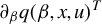
$\partial _\beta q(\beta ,x,u)^T$
 ,
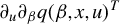
$\partial _u \partial _{\beta } q(\beta ,x,u)^T$
 , and
$\partial _{\beta _j} \partial _{\beta } q(\beta ,x,u)^T$
 (for
$j=1,\ldots ,\dim (\beta )$
 ) are Lipschitz in
$(\beta ,x,u)$
 . (vi)
$\partial _w G_\beta (w)$
 ,
$\partial _\beta G_\beta (w)$
 ,
$ \partial ^2_{\beta w^T} G_\beta (w)$
 ,
$\partial ^2_{w w^T} G_\beta (w)$
 ,
$\partial ^2_{\beta \beta ^T}G_\beta (w)$
 ,
$f_{W(\beta )}(w)$
 ,
$\mathbb {E}\{\varphi _s(X,H(Z))| W(\beta )=w\}$
 , and
$\partial _w\mathbb {E}\{\varphi _s(X,H(Z))|W(\beta )=w\}$
 are Lipschitz in
$(\beta ,w,s)$
 .
Assumption C. (i)
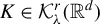
$K\in \mathcal {K}^r_{\lambda }(\mathbb R ^d)$
 with
$\lambda \geq \lceil (d+1)/2\rceil +6 $
 . (ii)
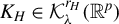
$K_H\in \mathcal {K}^{r_H}_\lambda (\mathbb R^p)$
 with
$\lambda \geq \lceil (p+1)/2 \rceil $
 . (iii)
$K_0\in \mathcal {K}^{r_0}_0(\mathbb R ^{\dim (X,Z)})$
 .
Let us define the following convergence rates:

The rate
$d_0$
 denotes the uniform convergence rate of the kernel density estimator
$\widehat {f}$
 . The rate
$d_H$
 is the uniform convergence rate of the first-step kernel density estimator
$\widehat {f}_Z$
 . Finally,
$d_G$
 is the uniform convergence rate of the third-step kernel density estimator if
$H(Z)$
 were observed.
Assumption D. (i)
$d_G h^{-1} \tau _n^{-3}=o(n^{-1/4})$
 and
$d_G h^{-|l|}\tau _n^{-2|l|}=o(1)$
 for
$|l|=\lceil (d+1)/2 \rceil +2$
 . (ii)
$d_H \tau _n^{-7} h^{-2}=o(n^{-1/4})$
 and
$d_H h_H^{-|l|}\tau _n^{-3-|l|}=o(1)$
 for
$|l|=\lceil (p+1)/2 \rceil $
 .
Since the framework is featured by generated regressors, we need some conditions on the rates at which the densities of the variables go to zero on the tails. So, let
$p_n^{W(\beta _0)}:=\Pr (f_{W(\beta _0)}(W(\beta _0))\leq 3 \tau _n /2)$
 ,
$p_n^Z:=\Pr (f_Z(Z)\leq 3 \tau _n /2)$
 ,
$p_n^{X,Z}:=\Pr (f(X,Z)\leq 3 \tau _n /2)$
 , and
$p_n:=\max (p_n^{W(\beta _0)}, p_n^Z, p_n^{X,Z})$
 . Also, let us define the sets

Assumption E. (i) For any
$\delta>0,$
 there exist
$\eta (\delta )>0$
 and
$N(\delta )$
 such that for all
$n\geq N(\delta )\ \mathcal {U}_n^\delta \subset \{(x,z)\,:\,q(\beta ,x,H(z))\in \mathcal {W}_{n,\beta }^{\eta (\delta )}\}$
 for all
$\beta \in B$
 and
$\mathcal {U}_n^\delta \subset \{(x,z)\,:\, z\in \mathcal {Z}_n^{\eta (\delta )}\}$
 . (ii)
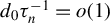
$d_0 \tau _n^{-1}=o(1)$
 ,
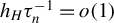
$h_H \tau _n^{-1}=o(1)$
 , and
$h \tau _n^{-1}=o(1)$
 . (iii)
$p_n=o(n^{-1/2})$
 ,
$p_n h^{-d-1}\tau _n^{-3}=o(n^{-1/4})$
 ,
$p_n h^{-|l|-d}\tau _n^{-1-|l|}=o(1)$
 , and
$p_n h_H^{-p} h^{-1-|l|}\tau _n^{-4-|l|}=o(1) $
 for
$|l|=\lceil (d+1)/2 \rceil +2 $
 . (iv)
$p_n h_H^{-p}h^{-2}\tau _n^{-6}=o(n^{-1/4})$
 and
$p_n h^{-p-|l|}_H\tau _n^{-2-|l|}=o(1)$
 for
$|l|=\lceil (p+1)/2 \rceil $
 . (v) For any
$\delta ,$
 there exists
$N(\delta )$
 such that
$\mathcal {W}_{n,\beta _0}^\delta $
 and
$\mathcal {Z}_n^\delta $
 are convex for all
$n\geq N(\delta )$
 .
Assumption F. (i) B is a compact convex set with non-empty interior, and
$\arg \min _{\beta \in B} \mathbb {E}\{Y-G_\beta (W(\beta ))\}^2=\{\beta ^*\}$
 for some
$\beta ^*\in \mathrm {Int}(B)$
 . (ii)
$\mathbb {E}\{G_{\beta _1}(W(\beta _1))| W(\beta _2)=w\}$
 is Lipschitz and uniformly bounded in
$(\beta _1,\beta _2,w)$
 . (iii)
$\Sigma $
 is full rank.
Let us now comment on the assumptions. Assumption A(ii) is an index restriction satisfied in the applications of our test described in Section 4. In general, such an index restriction is implied by distributional assumptions on unobservables that can be justified by economic arguments (see Section 4 for details). Note that under Assumption A(ii), the null in (3) is equivalent to
$\mathbb {E}\{Y|X,Z\}=\mathbb {E}\{Y|q(\beta _0,X,H(Z))\}$
 . We focus on the formulation in (3) because it helps reduce the curse of dimensionality in the test statistic, since typically
$\mathrm {dim}(\nu(X,H(Z)))$
 . Assumption A(iii) implies that, conditional on
$\nu (X,H(Z))$
 ,
$W(\beta )$
 is deterministic. Such an assumption holds in the applications of our test described in Section 4.
Assumption A(iv) and (v) set the conditions that the set
$\mathcal {S}$
 and the weighting function
$\varphi _s$
 must satisfy to guarantee the equivalence between the conditional moment restriction in (5) and the continuum of unconditional moment restrictions in (6). Bierens (Reference Bierens2017, Thm. 2.2) shows that Assumption A(iv) and (v) and the boundedness of
$\nu (X,H(Z))$
 (implied by Assumptions A(i), B(iii), and B(v)) are sufficient for such an equivalence to hold. Several choices of
$\varphi _s$
 have already been discussed in Section 2. Alternatively, the equivalence between the conditional moment restriction in (5) and the continuum of unconditional moment restrictions in (6) can be obtained by the results in Andrews and Shi (Reference Andrews and Shi2013), who construct weighting functions to transform conditional moment inequalities into unconditional moment inequalities. For simplicity and space reasons, we only consider weighting functions satisfying Assumption A(iv) and (v).Footnote
10
Assumption B imposes smoothness conditions that are common in the literature on semi and nonparametric testing.
Assumption D sets the main conditions on the bandwidths for the first-step estimation of H and the third-step estimation of
$G_{\beta _0}$
 . These conditions have a twofold role. First, together with Assumptions B and C, they imply that the first-step estimator of H and the third-step estimator of
$G_{\beta _0}$
 belong, with probability approaching one, to a smooth class of functions with a bounded entropy. This is needed to obtain the asymptotic stochastic equicontinuity of the empirical process underlying the statistic
$S_n$
 . Second, the bandwidth conditions in Assumption D guarantee that the first-step estimator
$\widetilde H$
 , the third-step estimator
$\widehat G _{\widetilde W (\widehat \beta )}$
 , and its first-order derivative
$\partial _w \widehat G _{\widetilde W (\widehat \beta )}$
 have an
$n^{-1/4}$
 convergence rate toward their targets. While the
$n^{-1/4}$
 consistency of the nonparametric estimators is common in the literature on semiparametric testing, the
$n^{-1/4}$
 consistency of the first-order derivative of
$\widehat G _{\widetilde W (\widehat \beta )}$
 is specific to our framework with generated regressors. Heuristically, to handle the estimation error from the generated regressor
$\widetilde H(Z)$
 , we combine the
$n^{-1/4}$
 consistency of the first-step estimator
$\widetilde H$
 with the
$n^{-1/4}$
 consistency of the third-step derivative
$\partial_w \widehat G _{\widetilde W (\widehat \beta )}$
 to obtain a first-order approximation of the type

The above expansion allows us to disentangle the estimation error coming from the third step and the estimation error due to the generated variable
$\widetilde H(Z)$
 .
An important aspect is that Assumption D avoids undersmoothing and allows for a small bias property of the empirical process underlying
$S_n$
 . To explain these features, let us abstract from the trimming rate
$\tau _n$
 . Then, Assumption D requires that
$n h^{4(r-1)}=o(1)$
 and
$n h_H^{4 r_H}=o(1)$
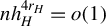 . These conditions have two consequences. First, we avoid undersmoothing, in the sense that the test can be implemented with bandwidths that are “optimal” for estimation.Footnote
11
Second, the empirical process
$ \mathbb{P}_n \,\widetilde{\varepsilon}\,\widehat{f}_{\widetilde{W}(\widehat{\beta})}(\widetilde{W}(\widehat{\beta}))\,\varphi_s(X,\widetilde{H}(Z))\,\widehat{t}$
 underlying the statistic has a small bias property. This means that such an empirical process remains
$\sqrt {n}$
 -consistent although the biases of the nonparametric estimators on which it is based do not vanish at an
$n^{-1/2}$
 rate. See Proposition 2.2(i) below and Newey et al. (Reference Newey, Hsieh and Robins2004). This feature is possible thanks to the bias corrections (or, equivalently, the
$L_2$
 boosting corrections) used in the first- and third-step estimation. Without such bias corrections, the conditions
$n h^{4(r-1)}=o(1)$
 and
$n h_H^{4 r_H}=o(1)$
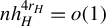 should be “augmented” by
$n h^{2\,r}=o(1)$
 and
$n h_H^{2 r_H}=o(1)$
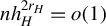 to guarantee that the bias of the empirical process vanishes quickly enough (see, e.g., Delgado and Manteiga, Reference Delgado and Manteiga2001; Escanciano et al., Reference Escanciano, Jacho-Chávez and Lewbel2014). With such rates, we would have to use undersmoothed bandwidths, and the empirical process underlying
$S_n$
 would no longer have a small bias property without undersmoothed bandwidths.
As highlighted earlier, Newey et al. (Reference Newey, Hsieh and Robins2004) develop a technique based on twicing kernels to achieve a small bias property in the context of semiparametric estimation when all regressors are observed. The bias corrections used here are similar to those used in Xia et al. (Reference Xia, Li, Tong and Zhang2004) and Lapenta and Lavergne (Reference Lapenta and Lavergne2025) who develop tests where all regressors are observed. Here, we show that these bias corrections (or, equivalently, the
$L_2$
 boosting corrections) guarantee a small bias property in a semiparametric context characterized by the presence of nonparametrically generated regressors.Footnote
12
The small bias property of the empirical process does not only have a theoretical appeal, but it is also attractive from a practical point of view: as we show in Section 5.2, this property implies that when the bandwidth is perturbed our test is more stable in terms of size than a test without the small bias property (see also Xia et al., Reference Xia, Li, Tong and Zhang2004). In other words, from a practical standpoint, thanks to the small bias property, we avoid an excessive sensitivity of the test with respect to the smoothing parameter.
Assumption E(i) is similar to Assumption 7 in Escanciano et al. (Reference Escanciano, Jacho-Chávez and Lewbel2014). It has a technical nature and essentially avoids the introduction of multiple trimmings. Specifically, to control for the random denominators present in
$\widetilde H$
 ,
$\widetilde G_{\widetilde W(\beta )}$
 , and
$\widehat G_{\widetilde W(\beta )}$
 , we should have introduced multiple trimmings, one for each random denominator in each estimator. By avoiding the introduction of multiple trimmings, Assumption E(i) dramatically simplifies the proofs.Footnote
13
Assumption E(ii)–(iv) gathers the conditions guaranteeing that the trimming disappears fast enough to avoid a bias coming from trimming. Similar conditions can be found in Escanciano et al. (Reference Escanciano, Jacho-Chávez and Lewbel2014). Assumption E(v) implies a convexity feature needed to limit the entropy of the class of functions that asymptotically contains the nonparametric estimators.
Finally, Assumption F imposes the existence of a unique pseudo-true value of the finite-dimensional parameter
$\beta _0$
 . Such a condition is common to any specification test for nonlinear models where the finite-dimensional parameter is estimated by optimizing a nonlinear objective function (see Bierens, Reference Bierens1982). Assumption F plays a double role: under
$\mathcal H _0$
 , it ensures the identification of
$\beta _0$
 , while, under
$\mathcal H _1$
 , it ensures that the estimator
$\widehat \beta $
 has a well-defined limit in probability. Now, under
$\mathcal H_0$
 , Assumption F can be verified using normalization conditions on B and support conditions on
$(X,Z)$
 . A common normalization condition is that the first component of
$\beta _0$
 , or, equivalently, the first coordinate of B, is normalized to one (see Blundell and Powell, Reference Blundell and Powell2004; Rothe, Reference Rothe2009; Escanciano et al., Reference Escanciano, Jacho-Chávez and Lewbel2016). Differently, under
$\mathcal H_1$
 , what is needed for our test to have power is a well-defined limit in probability of
$\widehat \beta $
 . We could directly impose these conditions, but we choose to keep Assumption F for presentation purposes.
The following proposition shows the IFR of the empirical process underlying the statistic
$S_n$
 .
Proposition 2.2. Let Assumptions A–F hold. Then, under
$\mathcal H _0$
 ,

uniformly in
$s \in {\mathcal {S}}$
 .
The above proposition is proved in Appendix A. A similar IFR is obtained in Escanciano et al. (Reference Escanciano, Jacho-Chávez and Lewbel2014), but under different conditions on the bandwidths and using different estimators. In particular, compared with Escanciano et al. (Reference Escanciano, Jacho-Chávez and Lewbel2014), our estimators include bias corrections and our empirical process exhibits a small bias property. Accordingly, the way we handle the bias terms appearing in the expansion of our empirical process is fundamentally different from the methods used in Escanciano et al. (Reference Escanciano, Jacho-Chávez and Lewbel2014).
The IFR obtained in Proposition 2.2 allows us to get more insights on the connection between the small bias property of our empirical process and the presence of generated variables. The second term in the IFR of the empirical process is due to the generated variable: the fact that we replace the unobserved regressor
$H(Z)$
 with the generated regressor
$\widetilde H (Z)$
 introduces additional terms in the first-order asymptotics of our empirical process. Thus, the initial empirical process is not locally robust with respect to the first-step estimation, in the sense that the Gateaux derivative of the moment condition in (6) with respect to H is nonzero. In other words, such a moment condition is not Neyman-orthogonal with respect to the first-step estimation (see Chernozhukov et al., Reference Chernozhukov, Escanciano, Ichimura, Newey and Robins2022). Now, as an alternative to the bias (or
$L_2$
 boosting) corrections, we could obtain a small bias property for our empirical process using a “locally robust” approach, as proposed in Chernozhukov et al. (Reference Chernozhukov, Escanciano, Ichimura, Newey and Robins2022). This would require estimating the second term appearing in the IFR of Proposition 2.2 (due to the generated variable) and adding this adjustment term to the empirical process underlying
$S_n$
 . The new empirical process would be “locally robust,” in the sense that it would be the empirical counterpart of a moment condition whose Gateaux derivative with respect to H is zero. Then, as a test statistic, we could consider the Cramér–von Mises functional of such a locally robust empirical process. This new empirical process would exhibit a small bias property like ours (see Chernozhukov et al., Reference Chernozhukov, Escanciano, Ichimura, Newey and Robins2022, for further details). However, the implementation of such a locally robust approach in our semiparametric framework with generated variables would be difficult. Constructing a locally robust empirical process would require estimating the terms
$a_s$
 ,
$b_s^1$
 , and
$b_s^2$
 . This, in turn, would require (i) selecting additional smoothing parameters and (ii) estimating the nonparametric derivatives
$\partial _w G _{\beta _0}$
 and
$\partial _\beta G _{\beta _0}$
 . Since, in practice, it is not convenient to estimate nonparametric derivatives, such an estimation would complicate the practical implementation of the test. Differently, our
$L_2$
 boosting procedure does not require estimating nonparametric derivatives. Thus, we are proposing an attractive and convenient method to achieve the small bias property in a semiparametric context with generated variables.
From Proposition 2.2, we obtain the asymptotic distribution of
$S_n$
 under
$\mathcal H _0$
 . Since
$\varphi _s$
 is Lipschitz in s, the class of functions indexing the IFR in Proposition 2.2 is Donsker. Hence, the empirical process underlying the statistic will converge weakly to a tight zero-mean Gaussian process
$\{\mathbb G_s\}_{s\in \mathcal {S}}$
 valued in
$\ell ^\infty (\mathcal S)$
 , with
$\ell ^{\infty }(\mathcal S)$
 denoting the space of uniformly bounded functionals over
$\mathcal S$
 . The Gaussian process
$\{\mathbb{G}_s\}_{s\in \mathcal {S}}$
 is characterized by the collection of covariances

Hence, by the continuity of the Cramér–von Mises functional, we obtain that, under
$\mathcal H _0$
 ,

A similar result also holds for the Kolmogorov–Smirnov statistic in (16), so that
$S_n^{KS}{\mathop {\longrightarrow }\limits ^{{d}}}\ \sup _{s\in \mathcal {S}}|\mathbb {G}_s|$
 . From the previous two displays, the asymptotic distribution of
$S_n$
 depends on the unknown DGP, and we cannot use it for testing.
This problem is often encountered in semiparametric testing. As noted in the previous section, Delgado and Manteiga (Reference Delgado and Manteiga2001) and Xia et al. (Reference Xia, Li, Tong and Zhang2004) test an equation similar to (6), but without generated variables. Their test statistics also converge to a functional of a zero-mean Gaussian process, and to obtain critical values they propose a bootstrap procedure. Differently from theirs, our context is featured by the presence of generated regressors. As shown in Proposition 2.2, the generated variables introduce an estimation error that affects the asymptotic behavior of our test statistic. Thus, the bootstrap procedures proposed in Delgado and Manteiga (Reference Delgado and Manteiga2001) and Xia et al. (Reference Xia, Li, Tong and Zhang2004) cannot be applied in our testing problem, as they cannot reproduce the estimation error induced by the generated regressors. Hence, in the next section, we motivate and develop a novel bootstrap procedure to construct the critical values.
3 THE BOOTSTRAP TEST
Before developing our bootstrap test, we discuss alternative methods that could be used to construct the critical values. This allows us to better motivate our bootstrap procedure. There are general methods available in the literature to adjust semiparametric tests for the presence of generated covariates (see Pagan, Reference Pagan1984; Wooldridge, Reference Wooldridge2010, Chap. 6; Hahn and Ridder, Reference Hahn and Ridder2013; Hahn et al., Reference Hahn, Liao and Ridder2018). They essentially work in two steps: (i) estimate the adjustment terms in the IFR of the statistic that are due to the generated variables and (ii) use these estimated adjustment terms to correct the “standard errors” of the test statistic and construct the critical values for the test. We could adapt such a procedure to our framework, but this would be difficult for two reasons. First, this general procedure applies to tests whose critical values are obtained from the asymptotic null distribution of the test statistic. However, obtaining the critical values from the asymptotic null distribution is not convenient in our framework, as it requires estimating an intricate collection of covariances (see the end of Section 2 for details). Second, given the IFR in Proposition 2.2, implementing such a procedure in our context requires estimating the weighting functions
$a_s$
 ,
$b_s^1$
 , and
$b_s^2$
 defined in (17). As noted in the previous section, this requires selecting additional smoothing parameters and estimating nonparametric derivatives. So, such a procedure would be practically difficult to implement in our context for the reasons discussed earlier.
A second alternative would be to construct a weighted bootstrap procedure, see Delgado and Manteiga (Reference Delgado and Manteiga2001). By letting
$\{\zeta _i\,:\,i=1,\ldots ,n\}$
 be a sequence of i.i.d. weights with mean zero, unit variance, and with a known distribution, the weighted bootstrap would be based on

where the “hatted” elements stand for estimated objects. The above process is a re-weighted version of the IFR in Proposition 2.2. Conditional on the sample data, the above process is expected to mimic the null behavior of the empirical process underlying our statistic. Thus, the idea would be to use it to construct valid critical values. However, this procedure is not attractive in our case: due to the presence of generated variables,
$a_s$
 ,
$b_s^1$
 , and
$b_s^2$
 involve nonparametric derivatives that must be estimated (see Equation (17)).Footnote
14
In view of the previous remarks, our goal in this section is to develop a bootstrap method that (i) does not require estimating nonparametric derivatives, (ii) reproduces the estimation error due to the generated regressors, (iii) resamples the observations by imposing the null hypothesis in the resampling scheme, and (iv) is based on an empirical process with a small bias property.
Let
$\{\xi _i\,:\,i=1,\ldots ,n\}$
 be i.i.d. copies of a random variable
$\xi $
 having a known distribution with
$\mathbb E \xi =0$
 and
$\mathbb E \xi ^2=1$
 , and let
$\{\xi _i\,:\,i=1,\ldots ,n\}$
 be independent from the sample data
$\{Y_i,X_i,Z_i,D_i\}_{i=1}^n$
 . The bootstrap DGP is

for
$i=1,\ldots ,n$
 . In the “bootstrap world,” only the weights
$\{\xi _i\,:\,i=1,\ldots ,n\}$
 are random and the sample data are fixed. The bootstrap sample is
$\{Y_i^*,D_i^{*},X_i,Z_i\}_{i=1}^n$
 . Below, we describe how to construct the bootstrap version of the statistic by using such a sample. For now, let us highlight some important features of the bootstrap DGP in (21). First, the bootstrap DGP consists of two equations. If there were no generated variables, the first equation alone would be enough to construct valid critical values. However, due to the presence of generated variables, a bootstrap DGP based only on the first equation would provide a misspecified inference, as it could not mimic the estimation error coming from the generated regressors. This is the reason for introducing the second equation in (21): its role is to reproduce the estimation error from the generated variable
$\widetilde H (Z)$
 , and to mimic the behavior of the second term in the IFR of Proposition 2.2.
Second, in some of the applications described in Section 4, the variable D is a component of X. Thus, D enters the true variable
$W(\beta _0)=q(\beta _0,X,H(Z))$
 in the population DGP. However, in the bootstrap DGP, the variable
$\widetilde W (\widehat \beta )=q(\widehat \beta ,X,\widetilde H (Z))$
 does not contain the bootstrap version of D, that is,
$D^*$
 , but only D. As we show in Proposition 3.1, this is sufficient to provide a valid bootstrap inference.
Third, the observations
$Y^*_i$
 and
$D^{*}_i$
 cannot be resampled independently, but they must be generated by the same bootstrap weight
$\xi _i$
 . This is an important feature, as it guarantees that the covariance of the bootstrap errors
$[Y^*_i-\widetilde G _{\widetilde W (\widehat \beta )}(\widetilde W _i (\widehat \beta )) , D^*_i - \widetilde H (Z_i)]$
 has the same structure as the covariance of the population errors
$[\,Y_i-G_{\beta _0}(W_i(\beta _0))\,,D_i-H(Z_i)\,]$
 . Since the former errors determine the behavior of the bootstrap version of
$S_n$
 and the latter errors determine the null behavior of
$S_n$
 , such a feature is fundamental to guarantee the validity of the bootstrap inference. See Proposition 3.1 ahead.
Fourth, unlike Xia et al. (Reference Xia, Li, Tong and Zhang2004), the bootstrap DGP in (21) involves the bias-corrected estimators. With this bootstrap DGP, we obtain a small bias property of the bootstrapped statistic since we bootstrap the bias corrections applied in the first- and third-step estimation; see below for details. By contrast, if we followed the approach of Xia et al. (Reference Xia, Li, Tong and Zhang2004) and did not bootstrap the bias corrections, we would need to include the uncorrected estimators in the bootstrap DGP of (21) to preserve the small bias property of the bootstrapped statistic.Footnote 15
Finally, we note that the bootstrap DGP in (21) guarantees the validity of the null hypothesis in the “bootstrap world.” In particular, let us denote with
$\mathbb E ^*$
 the expectation in the bootstrap world, where only the weights
$\{\xi _i\,:\,i=1,\ldots ,n\}$
 are random while the sample data are fixed. Then, (21) implies that
$\mathbb E ^* \{Y^*|\nu (X,\widetilde H (Z))\}=\mathbb E ^* \{Y^*|q(\widehat \beta , X,\widetilde H (Z))\}$
 . This equality represents the bootstrap version of
$\mathcal H _0$
 . The fact that we impose the null hypothesis in the bootstrap world is an attractive feature, as it means that we are using all the “available information” when resampling our observations. It also implies that, under the alternative, the critical values remain bounded, thus enhancing the power properties of the test.
Note that when D is discrete, its bootstrap counterpart
$D^*$
 from the bootstrap DGP in (21) will no longer be discrete. However, our bootstrap scheme remains valid.
In what follows, we show how to construct the bootstrap version of
$S_n$
 . Similarly to Section 2, this is done using a three-step procedure.
3.1 First-Step Estimation for the Bootstrap
Let

We use the trimming
$\widehat t$
 in the above expressions to control for the random denominators in
$D^{*}$
 and
$\widehat H^*$
 , see (21). Then, the bootstrap counterpart of
$\widetilde H$
 is

3.2 Second-Step Estimation for the Bootstrap
Let
$\widetilde W ^* _i (\beta ):=q(\beta ,X_i,\widetilde H ^* (Z_i))$
 . We define

and let
$\widehat f_{\widetilde W ^* (\beta )}$
 be defined similarly to Equation (11), with
$\widetilde W ^* (\beta )$
 replacing
$\widetilde W (\beta )$
 . Again, we use the trimming
$\widehat t$
 to control for the random denominator in
$Y^*$
 and
$\widetilde W ^*(\beta )$
 . Then, the bootstrap counterpart of
$\widehat G _{\widetilde W (\beta )}$
 is

Thus, we let the bootstrap counterpart of
$\widehat \beta $
 be

3.3 Third-Step Estimation for the Bootstrap
Let us define
$\widehat \varepsilon ^* _i := Y_i^* - \widehat G ^* _{\widetilde W ^* (\widehat \beta ^*)}(\widetilde W ^* _i (\widehat \beta ^*))$
 for
$i=1,\ldots ,n$
 . Let
$\widehat T ^{\widehat \varepsilon ^*}_{\widetilde W ^* (\beta )}$
 be defined similarly as in (24), obviously with
$\widehat \varepsilon ^*$
 replacing
$Y^*$
 . Then, the bootstrap counterpart of
$\widetilde G _{\widetilde W (\widehat \beta )}$
 is

The bootstrap counterpart of the bias-corrected residual is
$\widetilde \varepsilon ^*_i:=Y_i^*-\widetilde G ^*_{\widetilde W ^* (\widehat \beta ^*)} (\widetilde W ^*_i (\widehat \beta ^*))$
 . Hence, the bootstrap counterpart of the statistic is

Let us denote by
$\Pr ^*$
 the probability measure under which only the bootstrap weights
$\{\xi _i\,:\,i=1,\ldots ,n\}$
 are random, while the sample data are fixed. A test at the
$\alpha $
 nominal level is based on the quantile

In practice, one can compute
$\widehat c_{1-\alpha }$
 by a Monte Carlo procedure as follows:
-
1. Generate n i.i.d. bootstrap weights $\{\xi _i\,:\,i=1,\ldots ,n\}$
 from the distribution of
$\xi $
, and compute the observations
$\{Y_i^*,D^{*}_i\,:\,i=1,\ldots ,n\}$
as in (21).
-
2. Given the bootstrap sample $\{Y_i^*,D^{*}_i,X_i,Z_i\}_{i=1}^n$
, compute the test statistic
$S_n^*$
according to the three-step procedure described above. -
3. Repeat steps 1 and 2 $B^*$
times, with
$B^*$
large, and obtain the collection of bootstrapped statistics
$\{S^*_{n,b}\,:\,b=1,\ldots ,B^*\}$
. -
4. Compute $\widehat c_{1-\alpha }$
as the
$1-\alpha $
quantile of
$\{S^*_{n,b}\,:\,b=1,\ldots ,B^*\}$
.









If the statistic
$S_n$
 is larger than
$\widehat c_{1-\alpha }$
 , then the null hypothesis
$\mathcal H _0$
 is rejected at the
$\alpha $
 nominal level. We recommend choosing
$B^*$
 such that
$(1-\alpha )B^*$
 is an integer. The same procedure can be used to construct the bootstrap test based on the Kolmogorov–Smirnov statistic in (16).
The proposition below shows the validity of the bootstrap test just proposed. For brevity, we focus on the test based on the Cramér–von Mises statistic, but the same result holds for the test based on the Kolmogorov–Smirnov statistic
$S_n^{KS}$
 in (16).
Proposition 3.1. Let
$\{\xi _i\,:\,i=1,\ldots ,n\}$
 be an i.i.d. sequence of bounded random variables independent of the sample, with
$\mathbb E \xi =0$
 and
$\mathbb E \xi ^2=1$
 , and let Assumptions A–F hold. Then,
-
(i) under $\mathcal H _0$
, $$ \begin{align*} \sqrt{n}\, \mathbb P _n\, \widetilde \varepsilon^* \, \widehat f_{\widetilde W^*(\widehat \beta^*)}(\widetilde W^*(\widehat \beta^*))\, &\varphi_s(X,\widetilde H^*(Z))\, \widehat t\\&= \sqrt{n} \mathbb P _n\, \xi\,\varepsilon \, \left[f_{W(\beta_0)}(W(\beta_0))\,\varphi^\perp_s(X,Z) - b_s^1(X,Z) \right]\\&\quad - \sqrt{n} \mathbb P _n \, \xi\,(D - H(Z))\,\left[a_s(Z) - b_s^2(Z)\right] + o_P(1)\, \end{align*} $$
uniformly in $s\in \mathcal S$
, where the probability space is the joint probability on the random bootstrap weights and the sample data. -
(ii) Under $\mathcal H _0$
,
$\Pr (S_n> \widehat c_{1-\alpha })\rightarrow \alpha $
. -
(iii) Under $\mathcal H _1$
,
$\Pr (S_n> \widehat c_{1-\alpha })\rightarrow 1$
.





The above result is proved in Appendix C of the Supplementary Material. Let us comment on the bootstrap expansion obtained in Part
$(i)$
 .Footnote
16
The IFR of the bootstrapped empirical process is a reweighted version of the population IFR obtained in Proposition 2.2. The weights are represented by the bootstrap weights
$\{\xi _i\,:\,i=1,\ldots ,n\}$
 . Note that the covariance function of the bootstrapped IFR coincides with the covariance function in (19). This guarantees that, under
$\mathcal H _0$
 , the bootstrapped IFR will have the same behavior as the population IFR of Proposition 2.2. Thus, the bootstrapped statistic
$S_n^*$
 mimics the null behavior of
$S_n$
 , and the bootstrap inference is valid. For this property to hold, it is essential that the bootstrap weights in the two equations in (21) are the same.
Finally, we note that Proposition 3.1 is obtained under the bandwidth conditions of Assumption D. Thus, also the bootstrapped empirical process
$\mathbb{P}_n \,\widetilde{\varepsilon}^*\,\widehat{f}_{\widetilde{W}^*(\widehat{\beta}^*)}(\widetilde{W}^*(\widehat{\beta}^*))\,\varphi_s(X,\widetilde{H}^*(Z))\,\widehat{t}$
 underlying
$S_n^*$
 has a small bias property, in the sense that it remains
$\sqrt {n}$
 -consistent although the biases of the nonparametric estimators on which it is based do not vanish at an
$n^{-1/2}$
 rate.
4 MAIN APPLICATIONS
In this section, we present the main semiparametric models our test can be applied to.
4.1 Binary Choice Models with Control Functions
Control function methods are popular in econometrics for estimating binary choice models with endogenous regressors. They were first introduced by Rivers and Vuong (Reference Rivers and Vuong1988). They consider

where Y denotes the binary choice of an agent,
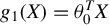
$g_1(X)=\theta _0^T X$
 for a parameter
$\theta _0$
 ,
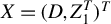
$X=(D,Z_1^T)^T$
 , and the unobserved error u is independent from
$Z_1$
 but correlated with D. To handle such a correlation, Rivers and Vuong (Reference Rivers and Vuong1988) assume that there exists an instrument
$Z_2$
 such that, for
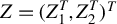
$Z=(Z_1^T,Z_2^T)^T$
 and an unobserved error ϵ,

The residual V is called control function, as it allows controlling for the endogeneity of D, and
$g_2(V,\epsilon )=-\gamma _0 V + \epsilon $
 . In addition to this structure, Rivers and Vuong (Reference Rivers and Vuong1988) assume that
$(\epsilon ,V)$
 are jointly normal and
$\mathbb E \{D|Z\}$
 is a linear function of Z. See also Section 4 in Wooldridge (Reference Wooldridge2015). More generally, one could consider a model given by (30) and (31), without imposing the normality of
$(\epsilon ,V)$
 and the linearity of
$\mathbb E \{D|Z\}$
 . This could be seen as a semiparametric version of Rivers and Vuong’s (Reference Rivers and Vuong1988) setting. This semiparametric version implies that
$\mathbb E \{Y|X,Z\}=\mathbb E \{Y|X,V\}$
 and that

The equation
$\mathbb E \{Y|X,Z\}=\mathbb E \{Y|X,V\}$
 is an exclusion restriction that is a direct consequence of (30) and the control function assumption in (31). It is obtained without imposing the parametric restrictions on
$g_1$
 and
$g_2$
 , and it can be justified by economic arguments. By contrast, the equation in the above display is implied by the parametric restrictions on
$g_1$
 and
$g_2$
 introduced to limit the curse of dimensionality. Our test can be applied to check the correct specification of such an equation. In particular, the equation in the previous display is a special case of Equation (3), where
$\nu (X,H(Z))=(X,D-H(Z))$
 ,
$q((\theta _0,\gamma _0),X,H(Z))=\theta _0^T X + \gamma _0(D-H(Z))$
 , and the generated variable is
$H(Z)=\mathbb E \{D|Z\}$
 .
In the same spirit, Blundell and Powell (Reference Blundell and Powell2004) consider a model given by Equation (30),
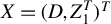
$X=(D,Z_1^T)^T$
 ,
$Z=(Z_1^T,Z_2^T)^T$
 , and the following exclusion restrictions:

where
$\sim $
 stands for equality in distribution, and V is as in (31). Moreover, they assume that
$g_1(X)=\theta _0^T X$
 for a parameter
$\theta _0$
 . The above display, (30), and the parametric structure of
$g_1$
 imply that
$\mathbb E \{Y|X,Z\}=\mathbb E \{Y|X,V\}$
 and that

The equation
$\mathbb E \{Y|X,Z\}=\mathbb E \{Y|X,V\}$
 is a direct consequence of (30) and the conditional independence restrictions in (32). It does not need the linear structure of
$g_1$
 . Hence, it can be justified by economic arguments. Differently, the parametric restriction on
$g_1$
 implies Equation (33). Such a restriction is introduced for convenience (i.e., to limit the curse of dimensionality) and cannot be justified by economic arguments. Our test can be used to check the validity of such a restriction. In particular, this restriction is a special case of (3), with
$\nu (X,H(Z))=(X,D-H(Z))$
 ,
$q(\theta _0,X,H(Z))=(\theta _0^T X,D-H(Z))$
 , and
$H(Z)=\mathbb E \{D|Z\}$
 , which is the generated variable.
4.2 Separable Single Index Models with Endogenous Regressors
Let Y be a continuous variable,
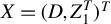
$X=(D,Z_1^T)^T$
 , and
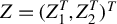
$Z=(Z_1^T,Z_2^T)^T$
 . Newey et al. (Reference Newey, Powell and Vella1999) consider the model

and
$V=D-\mathbb E \{D|Z\}$
 . Here,
$\epsilon $
 is an unobserved error term,
$G_0$
 is a nonparametric function,
$\beta _0$
 is a vector of parameters of interest, and D is an endogenous variable possibly correlated with
$\epsilon $
 . The second part of the above display is a mean-independence condition allowing to control for the endogeneity of D. Identification of
$G_0$
 and
$\beta _0$
 is discussed in Newey et al. (Reference Newey, Powell and Vella1999). Similarly to the previous section, this model implies that
$\mathbb E \{Y|X,Z\}=\mathbb E \{Y|X,V\}$
 and that
$\mathbb E \{Y|X,V\}=\mathbb E \{Y|X^T\beta _0,V\}$
 . The equation
$\mathbb E \{Y|X,Z\}=\mathbb E \{Y|X,V\}$
 does not depend on the index restriction on
$G_0$
 and is a direct consequence of the mean-independence condition in (34). Hence, it can be justified by economic arguments. By contrast, the equation
$\mathbb E \{Y|X,V\}=\mathbb E \{Y|X^T\beta _0,V\}$
 is a semiparametric restriction that can be checked by using our test, with
$\nu (X,H(Z))=(X,D-H(Z))$
 ,
$q(\beta _0,X,H(Z))=(\beta _0^T X,D-H(Z))$
 , and
$H(Z)=\mathbb E \{D|Z\}$
 , which is the generated variable.
4.3 Models with Sample Selection
Escanciano et al. (Reference Escanciano, Jacho-Chávez and Lewbel2016) consider a semiparametric model with sample selection and possibly truncation on the response variable. Let
$\widetilde Y \in \mathbb R$
 be a scalar random variable denoting an agent’s decision,
$(X,Z)$
 be a vector of covariates,
$D\in \{0,1\}$
 be a selection variable, and
$(\epsilon ,u)$
 be unobserved error terms. The model is

where
$\psi $
 is a known function,
$g(X)=\beta _0^T X$
 , but H is nonparametric. Without loss of generality, we can assume
$u\sim U[0,1]$
 , so H is identified as
$H(Z)=\mathbb E \{D|Z\}$
 and denotes the propensity score. Because of selection, only
$Y=\widetilde Y D$
 is observed. Let us denote by F the joint distribution of
$(\epsilon ,u)$
 . With F nonparametric, this setup is a semiparametric generalization of Heckman’s sample selection model. Setting
$\psi (g(X) ,\epsilon )=\mathbb I \{g(X) \geq \epsilon \}$
 yields a binary choice model with sample selection. If instead
$\psi (g(X) ,\epsilon )=\max \{0,g(X) + \epsilon \}$
 , we obtain a truncated regression model with sample selection. This model is also known as double hurdle model (see Escanciano et al., Reference Escanciano, Jacho-Chávez and Lewbel2016). Using the independence between
$(\epsilon ,u)$
 and
$(X,Z)$
 , we obtain
$\mathbb E \{Y|X,Z\}=\int \psi (g(X), \epsilon )\, \mathbb I \{H(Z)\geq u\} d\,F(u,\epsilon )$
 . Hence, the model implies
$\mathbb E \{Y|X,Z\}= \mathbb E \{Y|X,H(Z)\}$
 and

The equation
$\mathbb E \{Y|X,Z\}= \mathbb E \{Y|X,H(Z)\}$
 is obtained from (35) without assuming the linear structure of g. Differently, the equation in the above display comes from the parametric restriction on g. Such an equation can be tested using our procedure. Using the notation of Section 2, our test can be applied to this framework by setting
$\nu (X,H(Z))=(X,H(Z))$
 ,
$q(\beta _0,X,H(Z))=(\beta _0^T X, H(Z))$
 , and defining the generated variable as
$H(Z)=\mathbb E \{D|Z\}$
 .
4.4 Semiparametric Games with Incomplete Information
Aradillas-Lopez (Reference Aradillas-Lopez2012) and Lewbel and Tang (Reference Lewbel and Tang2015) study identification and estimation in binary games with incomplete information and linear payoffs. For simplicity, let us consider two players indexed by
$j\in \{1,2\}$
 . Each of them must take a binary decision, say
$a_j\in \{0,1\}$
 . Let
$X_j$
 be the vector of observed covariates entering agent j’s payoff function, and let
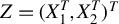
$Z=(X_1^T,X_2^T)^T$
 . Each player has a private information
$u_j$
 that neither the other player nor the researcher can observe. It is assumed that
$(u_1,u_2) \perp \!\!\!\perp Z$
 and
$u_1 \perp \!\!\!\perp u_2$
 . The payoff function of player j is

with
$g_j(X_j)=\gamma _j^T X_j $
 . We let
$H_j(Z)=\mathbb E \{a_j|Z\}$
 . Under the hypothesis that a unique Bayesian–Nash equilibrium is played, the model implies that
$\mathbb E \{a_j |X_1,X_2\}=\mathbb E \{a_j|X_j,H_{-j}(Z)\}$
 and that

for
$j=1,2$
 . The equation
$\mathbb E \{a_j |X_1,X_2\}=\mathbb E \{a_j|X_j,H_{-j}(Z)\}$
 follows directly from the assumption that a unique Bayesian–Nash equilibrium is played and does not need the linearity of the payoff function
$g_j$
 . Such an equation can be justified by economic arguments. Differently, the equation in the above display follows from a parametric restriction on
$g_j$
 . Our test can be used to check such a condition. In terms of the notation of Section 2, our test can be applied to this model by setting
$\nu (X,H(Z))=(X_j,H_{-j}(Z))$
 ,
$q((\gamma _j,\alpha _j), X_j,H_{-j}(Z))=\gamma _j^T X _j + \alpha _j \, H_{-j}(Z)$
 ,
$D=a_{-j}$
 , and
$H_{-j}(Z)=\mathbb {E}\{a_{-j}|Z\}$
 , which is the generated variable.
5 EMPIRICAL IMPLEMENTATION AND APPLICATIONS
In the first part of this section, we show how to implement our test in practice. In the second part, we study its behavior in small samples. Finally, in the third part, we apply our test to a real data example.
5.1 Implementation of the Test
To show the practical implementation of our test, we provide the computational details for the three-step procedure described in Section 2.1. Let us begin with the first step. The bandwidth for
$\widetilde H $
 is set according to Silverman’s rule of thumb, so
$h_H=\widehat {\sigma }_Z\, n^{-1/(2 r_H + p)}$
 , with
$\widehat \sigma _Z$
 denoting the estimated standard deviations of the components of Z and
$r_H$
 denoting the kernel order used for estimating H. The kernel
$K_H$
 is set to a second-order Gaussian kernel. Then, we compute
$\widetilde H $
 as in (10).
For the second step of Section 2.1, we need to compute the estimator
$\widehat \beta $
 by minimizing the objective function in (12). Note that the estimator
$\widehat G_{\widetilde W (\beta )}$
 in (12) depends on both
$\beta $
 and the bandwidth h. We follow the standard approach in semiparametric estimation (see, e.g., Escanciano et al., Reference Escanciano, Jacho-Chávez and Lewbel2016), and in practice we choose
$\widehat \beta $
 by solving the joint minimization problem

where
$\widehat G_{\widetilde W (\beta )}^{-i}$
 denotes the leave-i-out version of
$\widehat G_{\widetilde W (\beta )}$
 defined asFootnote
17

In the above expression, we set K to be a second-order Gaussian kernel.
$\widehat \beta $
 obtained from (36) is the estimator of
$\beta _0$
 .
Let us now describe the computational details of the third step of Section 2.1. To compute the statistic in (15), we need to select (i) a weighting function
$\varphi _s$
 , a measure
$\mu $
 , and a set
$\mathcal {S}$
 and (ii) a bandwidth h and a kernel K for
$\widetilde G_{\widetilde W (\widehat \beta )}$
 and
$\widehat f _{\widetilde W (\widehat \beta )}$
 . We select
$\varphi _s$
 ,
$\mu $
 , and
$\mathcal {S}$
 to make the computation of the integral in (15) fast and simple; see below for details. Thus, we set
$\varphi_s(X,H(Z))=\exp (\,\sqrt {-1}\,s^T\, \nu (X,H(Z))\,)$
 , let
$\mu $
 be the standard multivariate Gaussian density, and
$\mathcal {S}=\mathbb {R}^{\dim \nu (X,H(Z))}$
 . We set the kernel K to be a second-order Gaussian kernel. Finally, to choose the bandwidth h, we minimize the distance between the semiparametric model and the null hypothesis, so as to compute
$S_n$
 in an “optimistic” way. To this end, let us define the leave-i-out version of
$\widetilde G_{\widetilde W (\widehat \beta )}$
 as

where
$\widehat G ^{-i}_{\widetilde W (\widehat \beta )}$
 is defined in (37),
$\widehat f^{-i}_{\widetilde W (\widehat \beta )}$
 is the leave-i-out version of
$\widehat f_{\widetilde W (\widehat \beta )}$
 (defined similarly to (37)), and

Then, the bandwidth h for testing is selected as follows:

The intuition is simple: we are choosing the bandwidth for testing that makes the model “close” to
$\mathcal H _0$
 , where the distance is measured by a leave-one-out version of the Cramér–von Mises metric. The procedure can be seen as an adaptation of the cross-validation principle to our testing problem: while the cross validation chooses the bandwidth minimizing the distance between the leave-one-out residuals and zero, in our testing problem we choose the bandwidth to minimize the distance between the semiparametric model and the null hypothesis. This distance is measured by a leave-one-out version of the Cramér–von Mises functional. As we explain below, this way of choosing the bandwidth allows us to compare an “optimistic” statistic computed with the sample data to an “optimistic” statistic computed with the bootstrap data.Footnote
18
Thanks to the choice of
$\varphi _s$
 ,
$\mu $
 , and
$\mathcal {S}$
 , the integral in the optimization problem (39) has a simple closed-form expression given by

where
$\exp (-\|\cdot \|^2/2)$
 is the characteristic function of the standard multivariate normal. Since the above double sum depends on h in a highly nonlinear way, the optimization in (39) must be carried out numerically.
Once
$\widehat h$
 has been obtained from the minimization in (39), we can use it to compute the third-step estimators
$\widehat f _{\widetilde {W}(\widehat \beta )}$
 and
$\widetilde {G}_{\widetilde W (\widehat \beta )}$
 from (11) and (14). Thus, given the residuals
$\widetilde \varepsilon _i =Y_i - \widetilde G_{\widetilde W (\widehat \beta )}(\widetilde W_i (\widehat \beta ))$
 with
$i=1,\ldots ,n$
 , we compute the test statistic as

Let us now detail the computations for the bootstrapped statistic
$S_n^*$
 from Section 3. First, to generate bootstrap observations from (21), we need to define a distribution for the bootstrap weights
$\{\xi _i\,:\,i=1,\ldots ,n\,\}$
 . We suggest using a two-point Rademacher distribution:
$\Pr (\xi =1)=\Pr (\xi =-1)=1/2$
 . The choice of this distribution is motivated by its good performance in other contexts (see, e.g., Davidson and Flachaire, Reference Davidson and Flachaire2008). Then, given the bootstrap sample
$\{(Y_i^*,D_i^{*},X_i,Z_i)\, :\, i=1,\ldots ,n\}$
 obtained from (21), we use the same procedure as in the original sample to compute the bootstrap version of the test statistic,
$S_n^*$
 . Note that, for each bootstrap sample/iteration, we will have to minimize the bootstrap version of (36) to get
$\widehat \beta ^*$
 and the bootstrap version of (39) to get
$\widehat h ^*$
 . Finally, the critical values are obtained by the Monte Carlo procedure described in Section 3.
At this point, it is worth spending some words on the bandwidth selection procedure we have proposed. As previously highlighted,
$\widehat h$
 is selected to minimize the distance between the model and
$\mathcal H _0$
 . This gives an “optimistic” value of the sample statistic
$S_n$
 . However, also in the “bootstrap world” the bandwidth h is chosen to minimize the distance between
$\mathcal H _0$
 and the semiparametric model. Thus, also in the bootstrap world the statistic
$S_n^*$
 is computed with an optimistic view. Now, the optimistic view of
$S_n$
 will reflect the reality only when the null is true. Differently, the optimistic view of
$S_n^*$
 will always reflect the reality in the bootstrap world: since we are imposing the null
$\mathcal H _0$
 in the resampling scheme, the null is always satisfied in the bootstrap world. This implies that when
$\mathcal H _0$
 holds, the behavior of
$S_n$
 will reflect the behavior of
$S_n^*$
 , allowing to control the size of the test. By contrast, when the null hypothesis
$\mathcal {H}_0$
 does not hold,
$S_n$
 will be large as compared to the distribution of
$S_n^*$
 , and the test will reject
$\mathcal H _0$
 .
5.2 Small Sample Behavior
In this section, we study the small sample performance of our test in a Monte Carlo experiment. We specify a DGP in line with the binary choice model with a control function described in Section 4, and in particular, in Equations (30) and (31). Thus,

$(Z^{in}, Z^{ex} , V,\epsilon )$
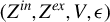 are mutually independent. The error terms
$(u,V,\epsilon )$
 are not observed. u is correlated with the endogenous regressor D through V, so V plays the role of a control function. The regressors
$Z^{in}$
 and
$Z^{ex}$
 are exogenous: the former is included in the equation for Y, while the latter is an excluded variable playing the role of an instrument. The control variable V is unobserved but can be estimated by estimating H. The functional form of H is unknown to the researcher, so H must be estimated nonparametrically.
We set
$V\sim \mathcal {N}(0,1)$
 ,
$\alpha =(1,1,1)/\sqrt {2}$
 , and
$Z^{in}\sim \mathcal {N}(0,1)$
 , and we draw
$Z^{ex}$
 from an exponential distribution truncated from above at 3 and standardized to have zero mean and unit variance. The parameter p controls the degree of departure from the null hypothesis; see below for details.
To check the robustness of our test with respect to different DGPs, we consider three different specifications for the distribution of
$\epsilon $
 :
-
DGP 1) $\epsilon \sim \mathcal {N}(0,sd=\sqrt {7});$
-
DGP 2) $\epsilon \sim \sqrt {7/(2\cdot 5)}\, (\chi _{5}^2 - 5);$
-
DGP 3) $\epsilon \sim 0.8\cdot \mathcal {N}(-2.5 , sd=\sqrt {3.5})+0.2\cdot \mathcal {N}(2.5,sd=1)$
.



DGP 1 yields a rescaled probit model with a distribution of
$\epsilon $
 that is unimodal and symmetric about zero. DGP 2 gives a unimodal distribution of
$\epsilon $
 with positive asymmetry and right skewness. Finally, DGP 3 generates
$\epsilon $
 according to a mixture of two Gaussians, resulting in a distribution of
$\epsilon $
 that is bimodal and right-skewed. The three distributions for
$\epsilon $
 and (40) are built so as to guarantee realistic features of the simulated data. Across these DGPs, it holds that
$\mathrm {Var} (u)\approx 8$
 , Corr
$(u,V)\approx 0.35$
 , Corr
$(u,D)\approx 0.25$
 , and
$\mathrm {Var} (D + Z^{in})\approx 4.5$
 .
We assume that the researcher specifies the model as

$V=D-\mathbb {E}\{D|Z\}$
 ,
$Z=(Z^{in},Z^{ex})$
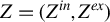 , and
$\epsilon \perp \!\!\!\perp (D,Z)$
 . The distribution of
$(\epsilon ,V)$
 is nonparametric. Similarly to Section 4, to check the correct specification of this model, the researcher needs to test

where
$X=(D,Z^{in})$
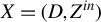 and
$H(Z)=\mathbb{E}\{D|Z\}$
 . Given the DGP in (40), the null hypothesis holds if
$p=0$
 . As long as
$p\neq 0 $
 , we are under the alternative
$\mathcal {H}_1$
 . The magnitude of p measures the degree of departure from the null hypothesis.
In the remainder of this section, our goal is threefold. First, we want to analyze the practical advantages of the bias corrections in our statistic that guarantee the small bias properties of our test. Second, we want to check the capacity of our test to correctly control the size under
$\mathcal H _0$
 . Third, we want to analyze its power properties.
Let us start from the first task. To investigate the advantages of using bias corrections and having a small bias property of our statistic, we compare the performances of two tests under different bandwidth choices. The first test is the one proposed in this article that uses the bias-corrected estimators
$\widetilde H$
 and
$\widetilde G _{\widetilde W (\widehat \beta )}$
 . We call it BC Test. The second test employs the procedure described in this article, with the only exception that it does not use the bias-corrected estimators, but it employs the uncorrected estimators
$\widehat H$
 and
$\widehat G _{\widehat W (\widehat \beta )}$
 . We call this test UN Test. We compare the ability of these two tests to control the size under different bandwidth choices. So, in the third-step estimation, we use the bandwidth rule
$h=\,C\, \widehat \sigma (D + \widehat \theta Z^{in} + \widehat \gamma (D-\widetilde H (Z)))\, n^{-1/6}$
 , where
$\widehat \sigma $
 is the estimated standard deviation of its argument and C is a constant. This allows us to study the stability of each test under different bandwidth choices by letting the constant C vary over different values.Footnote
19
We run 10,000 simulations under the null
$\mathcal H _0$
 (i.e., by setting
$p=0$
 ) for
$n=400$
 and no trimming. Since the procedure is computationally intensive (see Section 5.1), we use the Warp-Speed method proposed by Davidson and MacKinnon (Reference Davidson and MacKinnon2007) and studied in Giacomini, Politis, and White (Reference Giacomini, Politis and White2013). This consists of drawing one bootstrap sample for each Monte Carlo simulation, and then using the entire set of bootstrapped statistics to compute the bootstrap p-values associated with each original statistic. We let the constant C vary in the range of values
$\{0.5,1,1.5,2,2.5\}$
 . For each of these values and for each simulated sample, the BC Test and the UN Test give two respective p-values and hence two respective decisions about the rejection of the null
$\mathcal H _0$
 . The results are reported in Figure 1 for DGP 1. For reasons of space, we omit the results for DGP 2 and DGP 3, as they are qualitatively similar to those for DGP 1. For each value of C, Figure 1 contains the error in rejection probability (ERP) of each test: this is the difference between the empirical rejection frequency and the nominal size of the test under the null
$\mathcal H _0$
 . An ideal test would display a null ERP for each nominal size and for each value of C. This comparison allows us to evaluate (i) the ability of each test in controlling the size under different bandwidth choices and (ii) the importance of employing bias corrections for estimating the null distribution of the statistic by wild bootstrapping. In other words, this gives us a measure of the stability (robustness) of each bootstrap test with respect to the bandwidth. For
$C=0.5$
 up to
$C=1,$
 both the BC Test and the UN Test display a good empirical size control for any nominal size. For
$C=1.5$
 and
$C=2$
 , the size control starts deteriorating for the UN Test, while it remains quite stable for the BC Test at any nominal size. This means that the bootstrap does not manage to provide a good estimation of the null distribution of the statistic when bias corrections are not employed. This feature becomes even clearer for
$C=2.5$
 : in this case, the UN Test exhibits a large ERP, while the BC Test shows a good size control for nominal levels up to 10%. These results show that employing bias corrections enables the bootstrap test to be stable with respect to the bandwidth choice. Also, these bias corrections allow for a satisfactory approximation of the null distribution of the statistic by our wild bootstrap procedure. Thus, such corrections do not only have the attractive theoretical feature of guaranteeing a small bias property of the test statistic, but they also have remarkable practical advantages.
Errors in rejection probabilities for the bias corrected and the uncorrected test.
Note: Error in rejection probability (= Empirical rejection frequency of the test − nominal size of the test) as a function of the nominal level for the bias corrected test (Bias Corr.) and the uncorrected test (Uncorr.). Each test is implemented with the bandwidth
$C h_S$
 , where
$h_S$
 is Silverman’s rule of thumb bandwidth and
$C\in \{0.5,1,1.5, 2, 2.5\}$
 . The sample size is
$n=400$
 .

Figure 1 Long description
Each of the five panels shares the same axes: the x-axis represents Nominal level from 0.0 to 0.5, and the y-axis represents Error in rejection probability from 0.0 to 0.6. A legend in the first panel identifies a solid blue line as Bias Corr. and a dash-dotted purple line as Uncorr. A horizontal dashed grey line at y equals 0 serves as a baseline.
* Top-left panel (C = 0.5): Both lines remain nearly flat and overlap closely with the zero baseline across the entire x-axis range.
* Top-right panel (C = 1): Both lines remain very close to the zero baseline, showing minimal error.
* Middle-left panel (C = 1.5): The Bias Corr. line remains flat at zero. The Uncorr. line begins to deviate upward starting at a nominal level of 0.15, reaching approximately 0.1 at the 0.5 mark.
* Middle-right panel (C = 2): The Bias Corr. line remains near zero. The Uncorr. line shows a significant upward curve starting at 0.05, rising steeply to reach an error of approximately 0.35 at the 0.5 mark.
* Bottom-center panel (C = 2.5): The Bias Corr. line shows a slight upward trend, reaching about 0.1. The Uncorr. line rises sharply from the origin, peaking at an error of approximately 0.55 around a nominal level of 0.3 before slightly declining toward 0.45.
Let us now turn to our second and third tasks. Here, we analyze the performance of our bias-corrected test in terms of size control and power properties when the third-step bandwidth h is selected as in (39). We label such a test as BC Test (
$\widehat h$
 ). We also study the performance of the bias-corrected Kolmogorov–Smirnov test based on (16). This test is implemented similarly to the three-step procedure described in Section 5.1. The third-step bandwidth is computed according to the “rule of thumb” and set to
$\widehat \sigma (D+\widehat \theta Z^{in}+\widehat \gamma (D-\widetilde H(Z)))\ n^{-1/6}$
 , while the weighting function is set to
$\varphi_s(X,\widetilde{H}(Z))=\exp ((1,\nu (X,\widetilde H(Z))^T)\,s)$
 with
$s\in \mathcal {S}'$
 and
$\mathcal {S}'=[-1/3,1/3]^{\dim (\nu (X,H(Z)))+1}$
 . We label such a test as KS-BC Test.Footnote
20
We run 10,000 Monte Carlo replications for
$n=400$
 and
$n=800$
 . Also in this case, the procedure is computationally intensive: we need to run a nonlinear optimization to obtain
$\widehat \beta $
 and a nonlinear optimization to obtain
$\widehat h$
 , for both the sample and the bootstrap data.Footnote
21
Thus, to speed up computations, we use the Warp-Speed method described above. We compute the empirical rejection frequencies for the BC Test (
$ \widehat h$
 ) and the KS-BC Test under
$\mathcal H _0$
 , that is, by setting
$p=0$
 . This allows us to evaluate the performance of the tests in terms of size control for each sample size. To investigate the influence of trimming, we compute the rejection probabilities both when no observation is trimmed and when the top 1% most extreme observations on
$(X,Z)$
 are trimmed.Footnote
22
The results are reported in Tables 1–3 for the nominal sizes of 5% and 10%. The tests show a good size control under
$\mathcal H _0$
 across the different DGPs considered, also for the limited sample size of
$n=400$
 . The rejection probabilities are not significantly affected by the amount of trimming and are stable with respect to the trimming parameter. To evaluate the performance of the tests in terms of power, we compute the rejection probabilities for
$p\in \{0.25,0.5,0.75,1\}$
 . Indeed, the larger p, the greater the departure from the null hypothesis. We display the results in Figures 2 and 3. The tests display a satisfactory power across the different DGPs, with our benchmark Cramér–von Mises test showing a larger power than the Kolmogorov–Smirnov test. For a given sample size, the power of each test increases as we depart from the null hypothesis, that is, when p increases. Similarly, for a given level of p, the power of each test increases as the sample size grows.
Empirical rejection frequencies of the tests for DGP 1.

Table 1 Long description
The table is organized into columns for Trimming and No trimming, each subdivided by nominal sizes of 0.05 and 0.10.
For n = 400:
* B C Test (h-hat): Trimming values are 0.0567 and 0.0996; No trimming values are 0.0546 and 0.0986.
* K S-B C Test: Trimming values are 0.0602 and 0.1014; No trimming values are 0.0564 and 0.1030.
For n = 800:
* B C Test (h-hat): Trimming values are 0.0471 and 0.0887; No trimming values are 0.0474 and 0.0908.
* K S-B C Test: Trimming values are 0.0506 and 0.0990; No trimming values are 0.0479 and 0.0915.
The B C Test refers to the Cramér-von Mises test with bias corrections, and the K S-B C Test refers to the Kolmogorov-Smirnov test with bias corrections. Data is based on 10,000 Monte Carlo replications.
Note: Empirical rejection frequencies of the tests for DGP 1 under
$\mathcal {H}_0$
 (corresponding to
$p=0$
 in (40)). BC Test (
$\widehat h$
 ) is the Cramér–von Mises test with bias corrections based on (15) and implemented with the bandwidth from Equation (39). KS-BC Test is the Kolmogorov–Smirnov test with bias corrections based on (16) and implemented with the “rule of thumb” bandwidth. The nominal sizes of the tests are in bold. The number of Monte Carlo replications is 10,000.
Empirical rejection frequencies of the tests for DGP 2.

Table 2 Long description
The table is organized into two main horizontal sections based on sample size n.
Top section for n = 400:
* Under Trimming 0.05: B C Test (h-hat) is 0.0485; K S-B C Test is 0.0495.
* Under Trimming 0.10: B C Test (h-hat) is 0.0965; K S-B C Test is 0.1004.
* Under No trimming 0.05: B C Test (h-hat) is 0.0520; K S-B C Test is 0.0515.
* Under No trimming 0.10: B C Test (h-hat) is 0.0999; K S-B C Test is 0.1015.
Bottom section for n = 800:
* Under Trimming 0.05: B C Test (h-hat) is 0.0472; K S-B C Test is 0.0457.
* Under Trimming 0.10: B C Test (h-hat) is 0.0933; K S-B C Test is 0.0890.
* Under No trimming 0.05: B C Test (h-hat) is 0.0470; K S-B C Test is 0.0445.
* Under No trimming 0.10: B C Test (h-hat) is 0.0909; K S-B C Test is 0.0893.
The nominal sizes 0.05 and 0.10 are highlighted as bold column headers. B C Test refers to the Cramer-von Mises test with bias corrections, and K S-B C Test refers to the Kolmogorov-Smirnov test with bias corrections.
Note: Empirical rejection frequencies of the tests for DGP 2 under
$\mathcal {H}_0$
 (corresponding to
$p=0$
 in (40)). BC Test (
$ \widehat h$
 ) is the Cramér–von Mises test with bias corrections based on (15) and implemented with the bandwidth from Equation (39). KS-BC Test is the Kolmogorov–Smirnov test with bias corrections based on (16) and implemented with the “rule of thumb” bandwidth. The nominal sizes of the tests are in bold. The number of Monte Carlo replications is 10,000.
Empirical rejection frequencies of the tests for DGP 3.

Table 3 Long description
The table is organized into two main header categories: Trimming and No trimming. Each category is further divided into nominal sizes of 0.05 and 0.10. The data is presented for two sample sizes, n = 400 and n = 800, for two specific tests: B C Test (h-hat) and K S - B C Test.
For n = 400:
* B C Test (h-hat): Trimming 0.05 is 0.0567, Trimming 0.10 is 0.1027; No trimming 0.05 is 0.0547, No trimming 0.10 is 0.0951.
* K S - B C Test: Trimming 0.05 is 0.0588, Trimming 0.10 is 0.1006; No trimming 0.05 is 0.0556, No trimming 0.10 is 0.0973.
For n = 800:
* B C Test (h-hat): Trimming 0.05 is 0.0409, Trimming 0.10 is 0.0929; No trimming 0.05 is 0.0456, No trimming 0.10 is 0.0965.
* K S - B C Test: Trimming 0.05 is 0.0448, Trimming 0.10 is 0.0919; No trimming 0.05 is 0.0451, No trimming 0.10 is 0.0951.
Note: Empirical rejection frequencies of the tests for DGP 3 under
$\mathcal {H}_0$
 (corresponding to
$p=0$
 in (40)). BC Test (
$ \widehat h$
 ) is the Cramér–von Mises test with bias corrections based on (15) and implemented with the bandwidth from Equation (39). KS-BC Test is the Kolmogorov–Smirnov test with bias corrections based on (16) and implemented with the “rule of thumb” bandwidth. The nominal sizes of the tests are in bold. The number of Monte Carlo replications is 10,000.
This simulation experiment shows that our benchmark bias-corrected bootstrap test, BC Test (
$ \widehat h$
 ), based on the empirical bandwidth selection in (39) controls well the size under
$\mathcal H _0$
 and has a satisfactory power. We also observe a good performance of the Kolmogorov–Smirnov-based test.
We conclude this section by investigating the finite sample behavior of the weighted bootstrap procedure based on the representation in (20).Footnote
23
As discussed in Section 3, implementing such a procedure is not convenient in our framework, as it requires estimating
$a_s$
 ,
$b_s^1$
 , and
$b_s^2$
 , all of which involve nonparametric derivatives. Since nonparametric derivatives have slow convergence rates in practice, such a procedure is expected to yield poor size control. For the practical implementation of the weighted bootstrap test,
$G_\beta $
 and H are estimated as in Section 2.
$a_s$
 ,
$b_s^1$
 , and
$b_s^2$
 , as well as the nonparametric derivatives appearing in them, are estimated by kernel smoothing, similarly to Section 2. The first-step bandwidth is the same as the one used for the benchmark test. The third-step bandwidth is chosen according to the “rule of thumb” and set to
$h=C \widehat \sigma (D+\widehat \theta Z^{in}+\widehat \gamma (D-\widetilde H(Z)))\,n^{-1/6}$
 , where C is a constant. We let C range in the set
$\{0.5, \, 1, \, 1.5\}$
 and obtain the rejection probabilities for each test corresponding to each C (i.e., bandwidth). Table 4 contains the simulation results. For reasons of space, we only report the results for DGP 1, as the results for DGPs 2 and 3 are similar. The weighted bootstrap yields a poor size control under the null hypothesis for a large range of bandwidths. This confirms the initial intuition about the behavior of such a test.
Power curves for the bias-corrected Cramér–von Mises test.
Note: Rejection probability as a function of the departure from the null hypothesis (p in Equation (40)) for the Cramér–von Mises bias-corrected test (BC Test (
$ \widehat h $
 )). The test is implemented with the bandwidth
$\widehat h$
 from (39) and no trimming. The sample sizes are
$n=400$
 and
$800$
 . The nominal size of the test is 10%.

Figure 2 Long description
A three-panel line graph titled D G P 1, D G P 2, and D G P 3 from left to right.
* Axes: Each panel shares the same axes. The x-axis is labeled p and ranges from 0.00 to 1.00. The y-axis is labeled Rejection Probability and ranges from 0.0 to 1.0. A horizontal dotted gray line is fixed at the 0.1 rejection probability level across all panels.
* Legend: Located in the top-left of the first panel, a solid blue line represents n equals 400 and a dashed red line represents n equals 800.
* D G P 1: Both curves start at 0.1 when p is 0.00. The dashed red line (n equals 800) shows a steep non-linear increase, reaching a probability of 1.0 at p equals 0.75. The solid blue line (n equals 400) shows a slower, more linear increase, reaching approximately 0.95 at p equals 1.00.
* D G P 2: Both curves start at 0.1. The dashed red line rises sharply to nearly 1.0 by p equals 0.50. The solid blue line shows an inflection point at p equals 0.25 before rising steeply to reach 1.0 at p equals 1.00.
* D G P 3: Similar to D G P 1, both curves start at 0.1. The dashed red line reaches 1.0 at p equals 0.75. The solid blue line follows a similar trajectory to D G P 1 but reaches a slightly higher final value closer to 1.0 at p equals 1.00.
Power curves for the bias-corrected Kolmogorov–Smirnov test.
Note: Rejection probability as a function of the departure from the null hypothesis (p in Equation (40)) for the Kolmogorov–Smirnov test based on bias corrections. The test is implemented with a “rule of thumb” bandwidth and no trimming. The sample sizes are
$n=400$
 and
$800$
 . The nominal size of the test is 10%.

Figure 3 Long description
A multi-panel figure with three line graphs labeled D G P 1, D G P 2, and D G P 3 from left to right.
All three graphs share identical axes. The x-axis is labeled p and ranges from 0.00 to 1.00. The y-axis is labeled Rejection Probability and ranges from 0.0 to 1.0. A horizontal dashed gray line at y equals 0.1 represents the nominal size of the test.
Each graph contains two curves. A solid blue line represents a sample size of n equals 400 and a dashed red line represents a sample size of n equals 800.
* In D G P 1, both curves start at 0.1 when p is 0. The n equals 800 curve shows a steep non-linear increase, reaching nearly 1.0 at p equals 0.75. The n equals 400 curve shows a more gradual linear-like increase, reaching 0.6 at p equals 1.0.
* In D G P 2, the n equals 800 curve rises even more sharply, reaching a plateau of 1.0 by p equals 0.75. The n equals 400 curve follows a convex path, reaching approximately 0.85 at p equals 1.0.
* In D G P 3, the trends are similar to D G P 1, where the n equals 800 curve approaches 1.0 at p equals 1.0, while the n equals 400 curve reaches approximately 0.75 at p equals 1.0.
In all panels, the n equals 800 curve consistently maintains a higher rejection probability than the n equals 400 curve for all values of p greater than 0.
Empirical rejection frequencies of the multiplier bootstrap tests for DGP 1.

Table 4 Long description
The table is organized into columns for sample size n, a parameter C, and two main categories of trimming: Trim = 1% and Trim = 2%. Each trimming category is further divided into nominal sizes of 0.05 and 0.10.
* For n = 400:
- When C = 1: Trim 1% values are 0.4818 and 0.6622; Trim 2% values are 0.4366 and 0.5914.
- When C = 1.5: Trim 1% values are 0.5608 and 0.7406; Trim 2% values are 0.5200 and 0.6830.
- When C = 0.5: Trim 1% values are 0.3646 and 0.5354; Trim 2% values are 0.2992 and 0.4700.
* For n = 800:
- When C = 1: Trim 1% values are 0.571 and 0.7284; Trim 2% values are 0.5068 and 0.6718.
- When C = 1.5: Trim 1% values are 0.6568 and 0.7980; Trim 2% values are 0.5860 and 0.7524.
- When C = 0.5: Trim 1% values are 0.4212 and 0.5972; Trim 2% values are 0.3518 and 0.5332.
Overall, rejection frequencies increase as the sample size n increases from 400 to 800 and as the nominal size increases from 0.05 to 0.10.
Note: Empirical rejection frequencies of the weighted bootstrap test for DGP 1 under
$\mathcal {H}_0$
 (corresponding to
$p=0$
 in (40)). The test is implemented using the bandwidth
$C h_S$
 for the third-step estimation, where
$h_S$
 is Silverman’s rule of thumb bandwidth. The column “
$Trim=1$
 %” (resp. “
$Trim=2$
 %”) contains the results of the test where 1% (resp. 2%) of the observations are trimmed. The nominal sizes of the tests are in bold. The number of Monte Carlo replications is 10,000.
5.3 An Application to Real Data
We illustrate the practical implementation of our procedure in a real data example. We test the specification of a semiparametric model describing women’s labor force participation (see Wooldridge, Reference Wooldridge2015). Such a model studies the impact of non-labor income on women’s labor force participation decisions. The data we use are taken from the 1991 wave of the Current Population Survey.Footnote
24
The sample consists of 2,947 women who do not have kids under the age of 6 and have a positive non-labor income. We set up the model and the notation similarly to Section 5.2. The dependent variable Y is an indicator that equals one if the woman participates in the labor force and 0 otherwise. D represents the household’s “other sources of income.” The vector of controls
$Z^{in}$
 includes the logarithm of the woman’s experience (
$Z^{in}_1$
 ) and a dummy indicating college or above education for the woman (
$Z^{in}_2$
 ). We treat D (other sources of income) as endogenous. Following Wooldridge (Reference Wooldridge2015), we set
$Z^{ex}$
 to the husband’s level of education. This is a dummy indicating college or above education, and it is used as an instrument to isolate the endogenous component of D. We normalize to unity the coefficient attached to D. We apply our test to assess the correct specification of three semiparametric index models, each similar to the one described in the previous section. First, we test the correct specification of the model in (41), where the linear index is
$D+\theta _0^T Z^{in}+\gamma _0(D-H(Z))$
 . We refer to this null hypothesis as
$\mathcal {H}_0(lin)$
 . Second, we test the correct specification of a model similar to (41), but with an added interaction term in the linear index:
$D+\theta _0^T Z^{in}+ \theta _1 Z^{in}_1\cdot Z^{in}_2+\gamma _0(D-H(Z))$
 . We denote this null hypothesis as
$\mathcal {H}_0(lin+int)$
 . Third, we test the correct specification of a further variation of (41), where we add a quadratic term in the linear index:
$D+\theta _0^T Z^{in}+ \theta _1 (Z^{in}_1)^2+\gamma _0(D-H(Z))$
 . We refer to this null hypothesis as
$\mathcal {H}_0(lin+quad)$
 .
To implement the tests in this real data example, we follow the steps described in Section 5.1. We apply the BC Test(
$\widehat h$
 ) with the bandwidth computed as in Equation (39). Note that the nonlinear optimization for the bandwidth has to be done with the sample data and for each bootstrap replication. The number of bootstrap iterations is set to
$B^*=999$
 . In Table 5, we report the value of the test statistic and the 99% bootstrap quantile for each specification test. Since the value of the statistic is above the 99% bootstrapped quantile for each specification test, each null hypothesis must be rejected at the 1% nominal level.Footnote
25
Test statistic and its 99% bootstrap quantile for the real data application.

Table 5 Long description
The table consists of three columns and four rows including the header.
Column headers from left to right:
1. Empty cell.
2. S sub n (Test statistic).
3. c-hat sub 0.99 (99 percent bootstrap quantile).
Data rows from top to bottom:
1. H sub 0 (l i n): S sub n is 1,229; c-hat sub 0.99 is 128.
2. H sub 0 (l i n plus i n t): S sub n is 1,279; c-hat sub 0.99 is 119.
3. H sub 0 (l i n plus q u a d): S sub n is 1,020; c-hat sub 0.99 is 109.
The table represents a B C Test with a sample size of 2,947 and 999 bootstrap replications.
Note: The test statistic
$S_n$
 and its 99% bootstrap quantile
$\widehat c _{0.99}$
 for the real data application. The test performed is the BC Test (
$\widehat h$
 ) with the bandwidth computed according to Equation (39). The sample size is 2,947, and the number of bootstrap replications is 999.
Appendix
This Appendix contains the proofs of the main results and additional technical material. Appendix A provides the proof of Proposition 2.2. The Supplementary Material contains Appendix B, which collects auxiliary lemmas for the proof of Proposition 2.2; Appendix C, which provides the proof of Proposition 3.1; Appendix D, which contains an auxiliary lemma for Proposition 3.1; Appendix E, which collects auxiliary technical lemmas used throughout the proofs; Appendix F, which provides an extension to models with semiparametrically generated regressors; and Appendix G, which provides implementation details for the weighted bootstrap procedure considered in the simulation study.
Notation: We use the notation
$\|g\|_{\infty ,\mathcal {A}}=\sup _{a\in \mathcal {A}}|g(a)|$
 for any function g defined on a set
$\mathcal {A}$
 . When the support of the argument of g is clear from the context, we simply denote
$\sup _{a\in \mathcal {A}}|g(a)|$
 with
$\|g\|_\infty $
 . We also use the convention that
$\widehat G _{\widetilde W (\widehat \beta )}(w)=\widehat T^Y_{\widetilde W (\widehat \beta )}(w)/\widehat f_{\widetilde W (\widehat \beta )}(w)$
 is set to 0 whenever
$\widehat f_{\widetilde W (\widehat \beta )}(w)=0$
 . The same convention applies to all other quantities involving a random denominator. We use the acronym “wpa1” to denote “with probability approaching one,” “RHS” to denote “right-hand side,” and “LHS” to denote “left-hand side.” In what follows, we write “uniformly in s” to mean “uniformly in
$s\in \mathcal {S}$
 .”
A PROOF OF PROPOSITION 2.2
Let
$t^\delta (x,z):=\mathbb {I}\{f(x,z)\geq \delta \tau _n\}$
 and
$\widehat t(x,z):=\mathbb {I}\{\widehat f(x,z)\geq \tau _n\}$
 . From Lemma E.3(ii) in the Supplementary Material, it follows that, wpa1,
$\widehat t (X_i,Z_i)\leq t^\delta (X_i,Z_i)$
 uniformly in
$i=1,\ldots ,n$
 , where
$\delta =1/2$
 . Assumption E(i) implies that there exists
$\eta (\delta )>0$
 such that
$t^\delta (X_i,Z_i)\leq \mathbb I \{f_{W(\widehat \beta )}(q(\widehat \beta ,X_i,H(Z_i)))\geq \eta (\delta )\tau _n\}$
 uniformly in
$i=1,\ldots ,n$
 , wpa1. Next, by Lemma E.3(iv) in the Supplementary Material, we obtain
$t^\delta (X_i,Z_i)\ \mathbb I \{f_{W(\widehat \beta )}(q(\widehat \beta ,X_i,H(Z_i)))\geq \eta (\delta )\tau _n\}\ \leq t^\delta (X_i,Z_i)\ \mathbb I \{f_{W(\widehat \beta )}(q(\widehat \beta ,X_i,\widetilde H (Z_i)))\geq \eta (\delta ) \tau _n/2\}$
 uniformly in
$i=1,\ldots ,n$
 , wpa1. In addition, Lemma E.3(iii) in the Supplementary Material implies that
$\mathbb I \{f_{W(\widehat \beta )}(q(\widehat \beta ,X_i,\widetilde H (Z_i)))\geq \eta (\delta ) \tau _n/2\}\ \leq \mathbb I \{\widehat f_{\widetilde W(\widehat \beta )}(q(\widehat \beta ,\ X_i,\widetilde H (Z_i)))\geq \eta (\delta ) \tau _n/4\}$
 uniformly in
$i=1,\ldots ,n$
 , wpa1. Collecting results, we obtain

uniformly in
$i=1,\ldots ,n$
 , wpa1. Thus, using the definition of
$\widetilde {G}_{\widetilde W (\widehat \beta )}$
 , we getFootnote
26

wpa1, where
$\widehat \varepsilon =Y-\widehat G_{\widetilde W (\widehat \beta )}(\widetilde W (\widehat \beta ))$
 and we omit
$(X,Z)$
 from the argument of
$\widehat t$
 for notational convenience. Next, define

In view of (A.1), we use the definition of
$\widehat {T}^{\widehat {\varepsilon }}_{\widetilde W (\widehat \beta )}$
 and exchange sums to obtain that the second term on the RHS of (A.2) equals
$\sqrt {n}\mathbb P _n\, \widehat {\varepsilon }\,\, \widehat {\iota }_s(\widetilde W (\widehat \beta ))\, \widehat {f}_{\widetilde W (\widehat \beta )}(\widetilde W (\widehat \beta ))\,\widehat {t}$
 wpa1. Thus, wpa1, the RHS of (A.2) equals

To prove the desired result, we derive the IFR for the RHS of the above display. We analyze each term separately. Let us start from the first one. By Lemma E.1(iii) in the Supplementary Material,
$|\widetilde H(Z_i)|(\widehat t _i + t_i)$
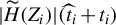 is bounded in probability uniformly in
$i=1,\ldots ,n$
 , where
$t_i:=\mathbb {I}\{f(X_i,Z_i)\geq \tau _n\}$
 . Thus,
$|\varphi _s(X_i,\widetilde {H}(Z_i))|(\widehat {t}_i+t_i)$
 is also bounded in probability uniformly in s and
$i=1,\ldots ,n$
 . Moreover, Lemmas B.2 and E.4(xiii) and (xv) in the Supplementary Material imply that
$|\widehat f_{\widetilde W (\widehat \beta )}(\widetilde W _i (\widehat \beta ))|(\widehat t_i + t_i)$
 and
$|\widehat \iota _s(\widetilde W _i (\widehat \beta ))|(\widehat t_i + t_i)$
 are bounded in probability uniformly in
$i=1,\ldots ,n$
 and s. Hence, since
$\widehat {t}-t=(\widehat {t}+t)(\widehat {t}-t)$
 , we obtain

where, in the last equality, we have used
$\sqrt {n}\mathbb {P}_n |\widehat t - t|=o_P(1)$
 from Lemma E.1(i) in the Supplementary Material, and we omit
$(X,Z)$
 from the argument of t and
$\widehat t$
 for notational convenience. Accordingly, in the first term on the RHS of (A.4), we may replace
$\widehat t$
 with t at the cost of an
$o_P(1)$
 remainder and obtain

uniformly in s. Now, Lemmas B.2 and E.1(iii) in the Supplementary Material ensure that
$\|\widehat {\beta }-\beta _0\|=O_P(n^{-1/2})$
 and
$\max _{i=1,\ldots ,n}\ |\widetilde {H}(Z_i)\ -H(Z_i)|t_i=o_P(n^{-1/4})$
 . Thus, by a mean-value expansion of
$q(\widehat {\beta },X_i,\widetilde {H}(Z_i))$
 around
$(\beta _0,X_i,H(Z_i))$
 and the Lipschitz continuity of
$\partial _{\beta ^T} q$
 and
$\partial _H q$
 (see Assumption B(v)), we getFootnote
27

uniformly in
$i=1,\ldots ,n$
 . This implies that
$\max _{i=1,\ldots ,n}|\widetilde W_i (\widehat \beta )-W_i(\beta _0)| t_i\ =O_P(\|(\widetilde H - H) t\|_\infty + \|\widehat \beta - \beta _0\|) =o_P(n^{-1/4})$
 .Footnote
28
Next, Lemma E.4(vii) and (ix) in the Supplementary Material ensures that both
$|\widehat f _{\widetilde W (\widehat \beta )}(W_i(\beta _0))|t_i$
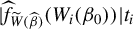 and
$|\widehat \iota _s(W_i(\beta _0))|t_i$
 are bounded in probability uniformly in
$i=1,\ldots ,n$
 and s. Using these results and substituting the stochastic expansions from Lemma E.6(ii)–(iv) in the Supplementary Material into (A.6), we obtainFootnote
29

uniformly in s. We now analyze the first term on the RHS of (A.8). For any
$\eta>0$
 , define

We obtain

uniformly in s. By Assumption E(i), there exists
$\eta>0$
 such that for all sufficiently large n,
$t_i\leq t_i\mathbb {I}\{f_{W(\beta _0)}(W_i(\beta _0))\geq \eta \tau _n \}$
 uniformly in
$i=1\ldots ,n$
 . This yields equality
$(a)$
 . Lemma E.4(x) in the Supplementary Material implies that
$|\widehat {f}_{\widetilde {W}(\widehat \beta )}(W_i(\beta _0))|\ t^\eta _{W(\beta _0)}(W_i(\beta _0))$
 is bounded in probability uniformly in
$i=1,\ldots ,n$
 . Hence, the second term on the RHS of equality
$(a)$
 is
$O_P(\sqrt {n} \mathbb P _n |t-1|)$
 . Since
$\sqrt {n} \mathbb P _n |t-1|=o_P(1)$
 from Lemma E.1(i) in the Supplementary Material, equality
$(b)$
 follows.
Note that, under
$\mathcal {H}_0$
 , the leading term on the RHS of equality
$(b)$
 in (A.10) is a centered empirical process. Lemma E.7(iv) in the Supplementary Material and Assumption B(i) ensure that
$\widehat {f}_{\widetilde {W}(\widehat \beta )} - f_{W(\beta _0)}\in \mathcal {G}_\lambda (\mathcal {W}_{n,\beta _0}^{\eta /2})$
 wpa1, where
$\lambda =\lceil (d+1)/2 \rceil $
 . Moreover, Lemma E.4(x) in the Supplementary Material implies that
$\|(\widehat {f}_{\widetilde {W}(\widehat \beta )}-f_{W(\beta _0)})t^\eta _{W(\beta _0)}\|_{\infty ,\mathcal {W}}=o_P(1)$
 . Thus, the stochastic equicontinuity result in Lemma E.10(i) in the Supplementary Material yields

uniformly in s. Finally, since
$\sqrt {n}\mathbb {P}_n|t^\eta _{W(\beta _0)}(W(\beta _0))-1|=o_P(1)$
 from Lemma E.3(i) in the Supplementary Material, we may replace
$t^\eta _{W(\beta _0)}$
 with 1 at the cost of an
$o_P(1)$
 remainder. Collecting results,

uniformly in s. Similar arguments yield

uniformly in s. Next, we analyze the third term on the RHS of (A.8). We obtain

uniformly in s. Equality
$(a)$
 follows from combining the
$n^{-1/4}$
 rates in Lemmas E.1(iii) and E.4(vii) in the Supplementary Material. Equality
$(b)$
 follows from the stochastic expansion in Lemma E.2(i) in the Supplementary Material and from
$\mathbb {E}\{\varepsilon |X,Z\}=0$
 under
$\mathcal {H}_0$
 (see Assumption A(ii)).
Let us now analyze the fourth term on the RHS of (A.8). We obtain, uniformly in s,

To obtain equality
$(a)$
 , we have used
$\max _{i=1,\ldots ,n}|\widetilde {W}_i(\widehat \beta ) - W_i(\beta _0)|t_i=o_P(n^{-1/4})$
 , as noted above, together with
$\max _{i=1, \ \ldots ,n}|\widehat {f}_{\widetilde {W}(\widehat {\beta })}(W_i(\beta _0))-f_{W(\beta _0)}(W_i(\beta _0))|t_i=o_P(n^{-1/4})$
 from Lemma E.4(vii) in the Supplementary Material. Equality
$(b)$
 follows from (A.7). For equality
$(c)$
 , Lemma E.1(i) in the Supplementary Material allows us to replace t with 1 in the first term on the RHS of equality
$(b)$
 , at the cost of an
$o_P(1)$
 remainder. Next, by Assumption B(vi),
$\sup _{(x,z)\in \mathrm {Supp}(X,Z)}\|\partial \iota _{s_1}(q(\beta _0,x,H(z)))-\partial \iota _{s_2}(q(\beta _0,x,H(z)))\|\leq C \|s_1-s_2\|$
 for all
$s_1,s_2\in \mathcal {S}$
 . Hence, by van der Vaart (Reference van der Vaart1998, Thm. 19.4 and Example 19.7), we obtain the following Glivenko–Cantelli result:

uniformly in s, where, for notational convenience, we omit
$W(\beta _0)$
 from the argument of
$f_{W(\beta _0)}$
 and
$\iota _s$
 . The expectation in the above display is zero, since
$\mathbb E \{\varepsilon |X,Z\}=0$
 under
$\mathcal {H}_0$
 (see Assumption A(ii)). Thus, since
$\sqrt {n}(\widehat \beta - \beta _0)=O_P(1)$
 from Lemma B.2 in the Supplementary Material, the first term on the RHS of equality
$(b)$
 in (A.13) is
$o_P(1)$
 . The second term on the RHS of equality
$(b)$
 is also negligible thanks to the expansion in Lemma E.2(i) in the Supplementary Material and
$\mathbb E \{\varepsilon |X,Z\}=0$
 under
$\mathcal H _0$
 . Thus, equality
$(c)$
 in (A.13) follows.
Arguing similarly to (A.13) yields

Collecting the previous results, we obtain, uniformly in s,

where
$\varphi _s^\perp (X,Z)=\varphi _s(X,H(Z))-\iota _s(W(\beta _0))$
 and we omit the argument of
$\varphi _s^\perp $
 for notational convenience.
In view of the above display, to obtain the desired result, it suffices to derive an IFR for the second term on the RHS of (A.4). Since
$\|(\widetilde H - H)\widehat t\|_\infty =o_P(n^{-1/4})$
 by Lemma E.1(iii) in the Supplementary Material, it follows from Assumptions A(v) and B(v) that
$|\varphi _s(X_i,\widetilde H (Z_i))-\varphi _s(X_i,H(Z_i))|\widehat t _i =O_P(\|(\widetilde H - H)\widehat t\|_\infty )=o_P(n^{-1/4})$
 uniformly in
$i=1,\ldots ,n$
 and s. Using this and the
$n^{-1/4}$
 rates in Lemma E.4(xiii)–(xv) in the Supplementary Material yields

uniformly in s, where, for notational convenience, we omit the argument of
$\varphi _s^\perp $
 . As in (A.5),
$\widehat {t}$
 may be replaced by t at the cost of an
$o_P(1)$
 remainder. Hence,

uniformly in s. Next, by Lemma E.6(i) in the Supplementary Material, we get

uniformly in s. For the first term on the RHS of (A.16), we obtain, uniformly in s,

where
$\eta>0$
 , and we omit
$W(\beta _0)$
 from the argument of
$t^\eta _{W(\beta _0)}$
 for notational convenience. Equality
$(a)$
 follows from the same arguments as in (A.10). To obtain equality
$(b)$
 , first note that the leading term on the RHS of equality
$(a)$
 is a centered empirical process, since
$\mathbb {E}\{\varphi _s^\perp (X,Z) |\ W(\beta _0)\}=0$
 . Moreover,
$G_{\beta _0}-\widehat {G}_{\widetilde {W}(\widehat \beta )}\in \mathcal {G}_\lambda (\mathcal W _{n,\beta _0}^{\eta /2})$
 wpa1, with
$\lambda =\lceil (d+1)/2\rceil $
 (see Lemma E.7(v) in the Supplementary Material and Assumption B(i)), and
$\|(\widehat {G}_{\widetilde {W}(\widehat {\beta })}-G_{\beta _0})t^\eta _{W(\beta _0)}\|_\infty =o_P(1)$
 (see Lemma E.4(xi) in the Supplementary Material). Hence, the stochastic equicontinuity result in Lemma E.10(i) in the Supplementary Material yields equality
$(b)$
 in the above display.
Finally, for the second term on the RHS of (A.16), we use arguments similar to those in (A.13) and obtain, uniformly in s,

Combining the previous five displays, we get

uniformly in s, where, for notational convenience, we omit the arguments of
$f_{W(\beta _0)}$
 ,
$\varphi _s^\perp $
 ,
$G_{\beta _0}$
 , and q. Finally, combining the above display, (A.4), (A.15), and the IFR of
$\sqrt {n}(\widehat \beta -\beta _0)$
 from Lemma B.2 in the Supplementary Material, we obtain the desired result.
${\blacksquare} $

SUPPLEMENTARY MATERIAL
The supplementary material for this article can be found at https://doi.org/10.1017/S0266466626100693.
FUNDING STATEMENT
This research has received financial support from the European Research Council under the European Community’s Seventh Program FP7/2007-2013 Grant Agreement No. 295298.
COMPETING INTEREST
The author declares that no competing interests exist.
























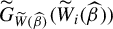

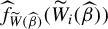



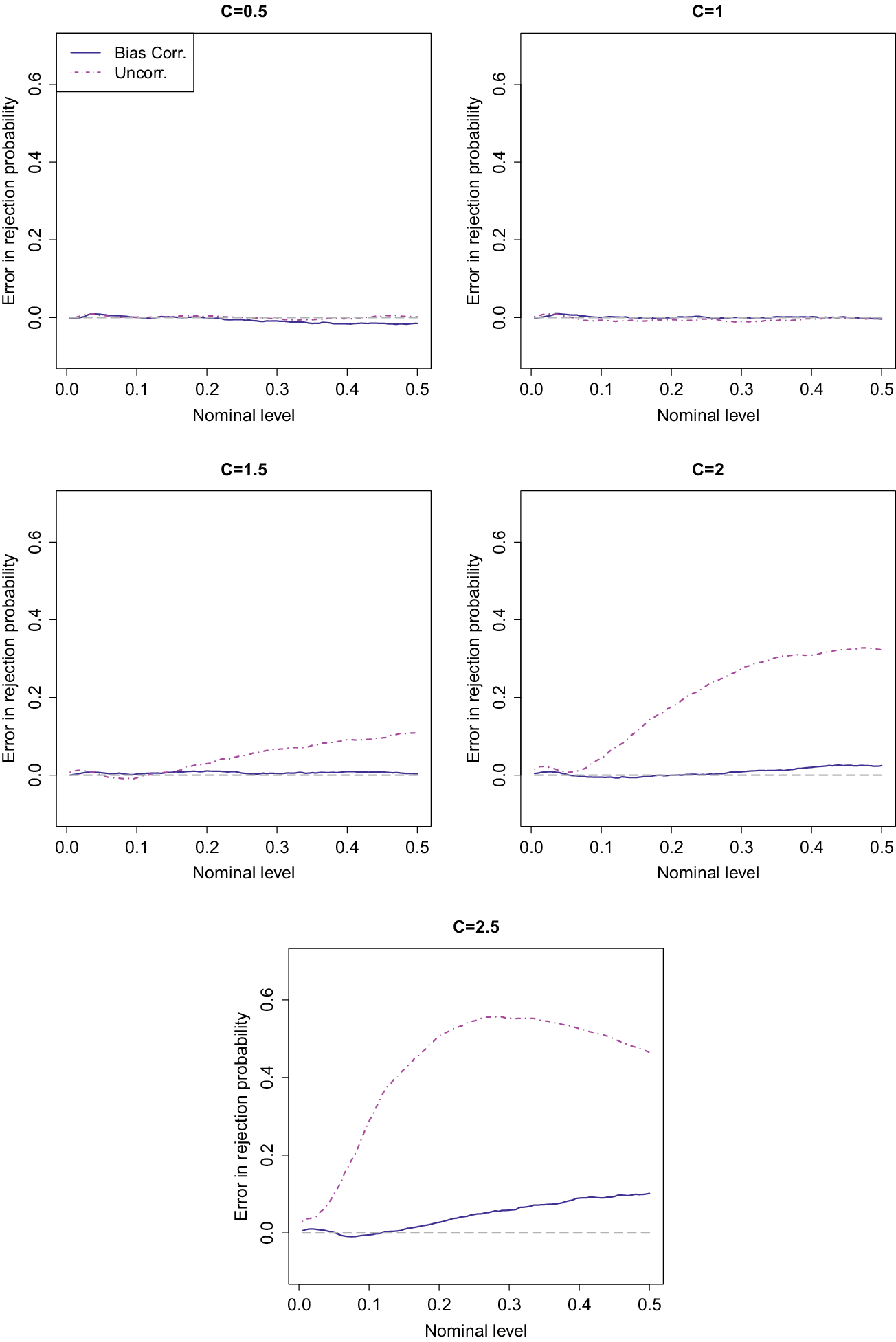


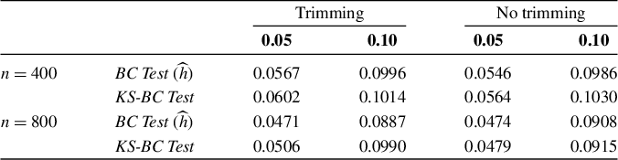
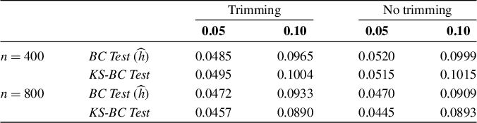
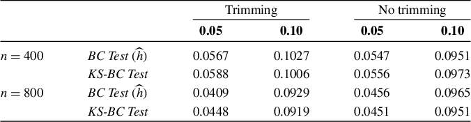
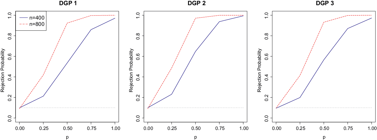


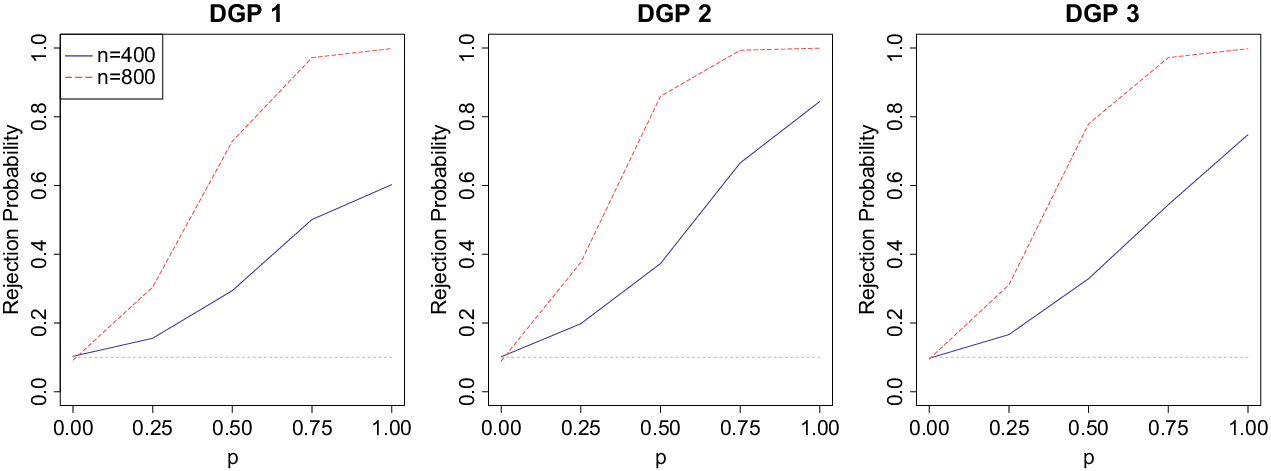


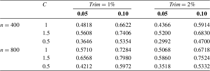
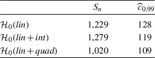


 Open access

