2.1. PI Processes

Consider a univariate time series x_sτ, where the first subscript refers to the season (s) and the second subscript to the year (τ). For simplicity of exposition, we assume data are quarterly and that observations are available for precisely N years, so that the total sample size is T = 4N, with initial values x₁₀ = x₂₀ = x₃₀ = x₄₀ = 0. The annual difference operator is Δ₄ = 1 − L⁴, where L is the usual lag operator that works on the seasons (L^kx_sτ = x_s−k,τ). Note that, throughout the paper, it is understood that x_s−k,τ = x_{4−k+s,τ−1} for s − k ≤ 0.

Applications of periodic processes within economics have focused on autoregressive (AR) processes, with the pth-order zero-mean periodic AR, or PAR(p), process defined by³

where e_sτ is white noise. Notice that all coefficients in (1) may vary with the season s. Although the conventional (nonperiodic) AR(p) process is a special case where φ_is = φ_i (s = 1, 2, 3, 4) for all i = 1,2,…, p, our interest is periodic processes, that is, cases where at least some of these nonperiodic parameter restrictions do not hold.

Under the assumption that x_sτ is integrated of order one, and using a similar notation to that of Boswijk and Franses (1996), (1) can also be written as

with φ₁φ₂φ₃φ₄ = 1. In the special case φ_s = 1 (s = 1,2,3,4), (2) is a periodic I(1) process, so that the first difference is a stationary PAR(p − 1) process. On the other hand, when φ₁φ₂φ₃φ₄ = 1 but not all φ_s = 1 (s = 1,2,3,4), (2) is a periodically integrated, or PI(1), process with the quasi-difference x_sτ − φ_s x_s−1,τ being stationary; see Ghysels and Osborn (2001, pp. 153–155) for further discussion of these cases. In the latter case x_sτ − φ_s x_s−1,τ may have constant coefficients over seasons, although for convenience we refer to it as a stationary PAR process.

In both the I(1) and PI(1) cases, nonstationarity arises from a single common trend shared by the four quarterly observations of the time series; equivalently, there are three cointegration relationships between the quarters. It is convenient to explore this through the representation referred to as the vector of quarters (VQ) representation by Franses (1994), which is based on the vector X_τ = (x_1τ,x_2τ,x_3τ,x_4τ)′ and disturbance process E_τ = (e_1τ,e_2τ,e_3τ,e_4τ)′. Corresponding to (1), the VQ representation has the form

where P = [(p − 1)/4] + 1 and [.] indicates the integer part of the expression in brackets. Corresponding to the factorization in (2), the VQ representation can be written as

where

and the determinant |Φ₀ − Φ₁ z| = 0 has a single unit root, while the stationary vector process Ψ(L⁴)U_τ = E_τ captures the stationary PAR(p − 1) process in u_sτ = x_sτ − φ_s x_s−1,τ embodied in (2).

From (3), the annual difference series Δ₄ X_τ = X_τ − X_τ−1 can be written as

where the vector process C(L⁴)U_τ = (Θ₀ − Θ₁ L⁴)U_τ has three noninvertible unit roots, which reflect the overdifferencing inherent in annual differencing for a process with a single AR unit root. Therefore, C(1) is of rank one, and it is possible to write

where a = (1,φ₂,φ₂φ₃,φ₂φ₃φ₄)′, b = (1,φ₁φ₃φ₄,φ₁φ₄,φ₁)′.

An implication of (4) and (5) is that the four elements of X_τ share a single common stochastic trend, namely,

, to which they adjust with periodic adjustment coefficients given by the elements of a. Further details can be found in Boswijk and Franses (1996).

2.2. Cointegration for PI Processes

Now consider the m × 1 vector process x_sτ = [x_sτ⁽¹⁾,…, x_sτ^(m)]′ in which each element is either a PI(1) or an I(1) process. That is,

in which each u_sτ^(j) is a stationary process (which is, in general, periodic)

with E_sτ = (e_sτ⁽¹⁾,…, e_sτ^(m))′ vector white noise and E [E_sτ E_sτ′] = Σ positive definite.⁴

Cointegration can then be defined as follows.

DEFINITION 1. The m × 1 vector x_sτ = [x_sτ⁽¹⁾,…, x_sτ^(m)]′ of periodic processes satisfying (6) is periodically cointegrated if there exist m × r matrices α_s of rank r such that the linear combinations α_s′x_sτ are (periodically) stationary for each s = 1,…,4.

Although it was not formally defined in this way, the idea of periodic cointegration appears to have been applied first by Birchenhall et al. (1989). Notice that nonperiodic cointegration, with α_s = α for s = 1, 2, 3, 4, is permitted here as a special case of periodic cointegration.

In their discussion of periodic cointegration, Boswijk and Franses (1995) distinguish full and partial periodic cointegration, where the former corresponds to Definition 1 and the latter to the situation where stationary linear combinations α_s′x_sτ exist for only some s = 1,…,4. However, Ghysels and Osborn (2001) show that partial periodic cointegration cannot apply between two PI(1) processes; such processes are either (fully) periodically cointegrated or no cointegrating relationship exists for any s = 1,…,4. This result is generalized in Lemma 1 for the case of m PI(1) processes.

LEMMA 1. Consider the m × 1 vector x_sτ = [x_sτ⁽¹⁾,…, x_sτ^(m)]′ of periodic processes in (6), such that the m × r matrix α_s of rank r defines all linearly independent stationary linear combinations α_s′x_sτ for some s = 1,…,4. Then

The first part of Lemma 1 implies that there must be the same number of cointegrating relationships between PI(1) processes for all seasons s = 1, 2, 3, 4. Thus, as in the bivariate case considered by Ghysels and Osborn (2001) and Osborn (2002), partial periodic cointegration cannot apply between PI(1) processes. Further, given the cointegrating vectors that apply for one season and the univariate PI coefficients of (1), then all four sets of cointegrating relations can be determined. It is worth noting that part (i) of Lemma 1 is implicit in the results of Kleibergen and Franses (1999), but they do not draw it out from their analysis.

Part (ii) of the lemma further establishes that the same (nonperiodic) cointegrating relations can apply over seasons if and only if all processes have identical univariate PI coefficients. The proof of this lemma rests on the fact that the VQ process corresponding to a PI(1) variable is driven by a single unit root process. The stationary relationships between observations for the seasons that exist for each X_τ^(j) = [x_1τ^(j),x_2τ^(j),x_3τ^(j),x_4τ^(j)]′ then imply that cointegrating relations for the vector x_sτ can be mapped from season to season.

Conventional cointegration between I(1) processes (which may be periodic) provides a special case of Lemma 1, where the same cointegrating relations apply for all seasons (quarters) of the year and all φ_s^(j) of (6) are unity.

2.3. Cointegration for SI Processes

Unlike the quasi-differencing x_sτ − φ_s x_s−1,τ of (2) with φ₁φ₂φ₃φ₄ = 1 that renders the PI(1) process stationary, SI(1) processes (that contain a unit root at the zero and each seasonal frequency) are made stationary and invertible by annual differencing. Such processes contain four unit roots, implying that the quarters of the year are not cointegrated with each other; Osborn (1991) and Franses (1994) provide discussions of some of the implications. In the context of cointegration between elements of an m × 1 vector x_sτ, if each element is SI(1) then the lack of cointegration across the seasons implies that distinct cointegrating relations can apply for each of the vectors x_sτ for s = 1,2,3,4. This is the essence of Lemma 2.

LEMMA 2. Consider the m × 1 vector x_sτ = [x_sτ⁽¹⁾,…, x_sτ^(m)]′ of SI(1) processes. Then the existence of an m × r matrix α_s of rank r such that α_s′x_sτ is stationary for some s = 1,…,4 has no implications for the existence or nature of cointegration across the elements of x_qτ for q ≠ s.

An immediate consequence of Lemma 2 is that full and partial periodic cointegration are possibilities for SI(1) processes.

So-called seasonal cointegration, which corresponds to cointegration at the distinct seasonal spectral frequencies, is another possibility for SI processes and is analyzed by Engle et al. (1993), Cubadda (2001), Johansen and Schaumburg (1999), and Lee (1992). However, our analysis focuses on testing for periodic cointegration. More specifically, we are particularly interested in testing for cointegration for PI processes. However, the case of SI processes is relevant, because Boswijk and Franses (1995) claim that the same asymptotic distribution results when their test is applied to both SI and PI processes.

3.1. The Test Regression

As usual, a residual-based test requires that the potential cointegrating relationship being examined is unique. That is, either there exists at most one cointegrating vector or, if there potentially exist 1 < r < m cointegrating vectors between the separate series, then (exclusion) restrictions are imposed to ensure uniqueness. From the analysis of the previous section, we know that cointegration applying for one season between PI processes implies cointegration for all seasons. Therefore, it is anticipated that efficiency gains will result by considering all seasons jointly.

To keep notation simple, we assume that only one cointegrating relationship may exist across the m variables. Arbitrarily normalizing on the first element of x, we propose fitting the periodic regression

and then applying the periodic integration test of Boswijk and Franses (1996) to the residuals

. The intuition is that, in the absence of cointegration, the residuals

follow a nonstationary PI process (see Franses, 1996, pp. 181–182).

Now, partition x_sτ as

so that z_sτ comprises the vector of right-hand-side variables in (7). We assume that all j = 1,…, m variables are PI(1) processes, as in (6), with the variance-covariance disturbance matrix corresponding to the system being

where Σ in (9) is partitioned conformably with x_sτ in (8).

3.2. Properties of the PI System

As discussed in Section 2.1, the matrix C^(j)(L⁴) in the representation of (4) for an annually differenced PI process has three unit roots, and hence

where a^(j) = [1, φ₂^(j), φ₂^(j)φ₃^(j), φ₂^(j)φ₃^(j)φ₄^(j)]′, b^(j) = [1, φ₁^(j)φ₃^(j)φ₄^(j), φ₁^(j)φ₄^(j), φ₁^(j)]′.

Stacking the processes, and using the annual difference representation of (4), yields

where Δ₄ X_τ = (Δ₄ X_τ⁽¹⁾′,Δ₄ X_τ⁽²⁾′,…, Δ₄ X_τ^(m)′)′, Δ₄ X_τ^(j) = (Δ₄ x_1τ^(j),Δ₄ x_2τ^(j), Δ₄ x_3τ^(j),Δ₄ x_4τ^(j))′, with corresponding definitions for E_τ^x and U_τ^x, while Ψ^x(L⁴) is a block diagonal matrix with jth block equal to Ψ^(j)(L⁴) containing the stationary (periodic) AR coefficients for series j. Similarly, the moving average (MA) coefficient matrices in (11) are block diagonal, of the form

and

The long-run covariance matrix between the m × 4 processes in X_τ is then given by (see also Boswijk and Franses, 1995, p. 440)

In the absence of cointegration between the x_sτ^(j)(j = 1,2,…, m), cointegration applies only across the seasons within each x_sτ^(j), and we have

where the 4m × m matrices a^x, b^x are defined by (in an obvious notation)

and all submatrices in (14) are 4 × 1. Thus, C^x(1) is of rank m.

However, if cointegration exists across processes, then C^x(1) is of rank k < m, and hence a^x and b^x do not have the block diagonal form of (14). Specifically, a^x and b^x are then matrices of rank k, with dimension 4m × k.

Returning to the case of no cointegration, Lemma 3, which follows, establishes the asymptotic distribution of the scaled vector X_τ = [X_τ⁽¹⁾′,Z_τ′]′ relevant for the regression (7). The result is obtained by accounting for the contemporaneous correlation between the disturbances through the decomposition Σ = PP′ where P is upper triangular.

LEMMA 3. Consider the vector of m PI(1) processes defined in (6), (8), (9), and (11), with no cointegration applying across the m processes. Also define the 4m × 1 vector Brownian motion W^x(r) with covariance matrix I_4m, where W^x(r) = [W⁽¹⁾(r)′,W^z(r)′]′ in which W⁽¹⁾(r) is 4 × 1, W^z(r) is 4n × 1, and n = m − 1. Then, as N = T/4 → ∞,

where [rN] is the integer part of rN, ρ_1z = σ₁₁^−1/2P_zz⁻¹σ_1z, the upper triangular matrix P_zz satisfies P_zz P_zz′ = Σ_zz, and a^z, b^z are the lower right-hand 4n × n blocks of a^x, b^x, respectively, in (14).

Here and throughout the paper ⇒ indicates convergence in distribution. Note that we can define standard Brownian motions underlying (15) as

where p^(j) is the (j − 1)th row of P_zz. Then, from (16), we can write

in which

Therefore, the scalar standard Brownian motions

in (16) can be thought of as the stochastic trends underlying the m individual PI processes, which in turn derive from the elements of the standard vector Brownian motion W^x(r).

It is clear from (15) or (16) that, in general, Brownian motions processes relating to x⁽¹⁾ and z are correlated. That is, when the contemporaneous covariance σ_1z in (9) is nonzero, W^z(r) influences

. This effect disappears in the special case of σ_1z = 0, because ρ_1z = 0 when x⁽¹⁾ is uncorrelated with x⁽²⁾,…, x^(m).

3.3. Asymptotic Distribution of the Test Statistic

We now turn to the properties of the residuals resulting from ordinary least squares (OLS) estimation of (7), which are summarized in Lemma 4.

LEMMA 4. Consider the vector of PI(1) processes defined in (6), (8), (9), and (11), with no cointegration applying across the m processes. The 4 × 1 vector

of residuals from (7) for year τ then satisfies, as N = T/4 → ∞,

where [rN] is the integer part of rN, l₁₁ is a scalar, ω = (b⁽¹⁾′Ψ⁽¹⁾(1)⁻¹ Ψ⁽¹⁾(1)′⁻¹b⁽¹⁾)^0.5, a⁽¹⁾ = [1,φ₂⁽¹⁾,φ₂⁽¹⁾φ₃⁽¹⁾,φ₂⁽¹⁾φ₃⁽¹⁾φ₄⁽¹⁾]′, b⁽¹⁾ = [1,φ₁⁽¹⁾φ₃⁽¹⁾φ₄⁽¹⁾, φ₁⁽¹⁾φ₄⁽¹⁾,φ₁⁽¹⁾]′, and the univariate Brownian motion w_m(r) is defined by

in which W^x(r) = [w⁽¹⁾(r),W^z(r)′]′ is m × 1 standard Brownian motion with covariance matrix I_m and k′ = [1,−∫w⁽¹⁾(r)W^z(r)′ dr(∫W^z(r)W^z(r)′ dr)⁻¹].

Lemma 4 implies that the residuals from (7) asymptotically retain the same nonstationary periodic coefficients as the univariate process for x_sτ⁽¹⁾ in (6). This is easily seen by comparing (18) with the first equation of (17).

Building on the implication of Lemma 4 that the residuals of (7) retain the PI properties of x_sτ⁽¹⁾ in (6), the strategy of testing for periodic integration in the residuals of (7) is clear. More specifically, following Franses (1996, pp. 181–182), we propose testing the periodic integration null hypothesis φ₁φ₂φ₃φ₄ = 1 against the alternative φ₁φ₂φ₃φ₄ < 1.⁵

Under the alternative hypothesis, the residuals of (20) are stationary, implying that either periodic cointegration or nonperiodic cointegration exists between the processes for all seasons s = 1, 2, 3, 4. Under the null hypothesis the residuals

, so that there is no cointegration between the PI processes. In this case, based on (6) and following Boswijk and Franses (1996), (20) can be reparameterized as

with the restriction φ₁φ₂φ₃φ₄ = 1 imposed, but ψ_js unrestricted, with estimation achieved using nonlinear least squares.

We employ the test of periodic integration proposed by Boswijk and Franses (1996), which uses the likelihood ratio (LR) statistic

where

is the unrestricted maximum likelihood estimator of Var(ε_sτ) in (20) and

is the corresponding estimator from (21) when the restriction φ₁φ₂φ₃φ₄ = 1 is imposed.

Theorem 1 establishes the asymptotic distribution of this periodic cointegration test statistic.

THEOREM 1. Under the null hypothesis of no cointegration between the PI processes of (6), (8), (9), and (11), the LR test statistic of (22) applied to the residuals from (7) using the PAR(p) regression (20)–(21) has asymptotic distribution

where w_m (r) is defined in (19) and k in Lemma 4.

The distribution of the test statistic in (23) is the square of the Dickey–Fuller test for cointegration using the residuals of a (nonperiodic) regression, as derived by Phillips and Ouliaris (1990). It is clear from (19) that this asymptotic distribution depends on the number of regressors in (7), namely, n = m − 1. Consequently, the distribution of the LR test statistic in (23) also depends on m. However, the distribution is invariant to the values of the PI coefficients for the processes in (6) and the disturbance covariances of (9).

Also in common with Phillips and Ouliaris (1990), the presence of stationary autocorrelation plays no role in the asymptotic distribution. However, in this periodic case, the augmentation in the test regression of (20)–(21) is periodic in form, because the possibility of stationary PAR dynamics is permitted under the null hypothesis.

5.1. Zero-Mean Processes

We investigate empirical size⁷

where the periodic components satisfy the univariate AR processes

and

The case of nonperiodic stationary components (31) is sufficient to illustrate the size and power properties of the test, with the processes being periodic through the PI coefficients in (30). Although results are presented only for stationary AR coefficients in (31) being common across the two processes, similar results have been obtained from simulations where these processes are distinct. Finally, it can be seen that (32) permits three levels of contemporaneous correlation between the innovations e_sτ^y and e_sτ^z.

As shown in Lemma 4, the data generating process (DGP) of (30) implies that the residuals follow a PI process when the regression of (7) is estimated.

Empirical power is obtained from the DGP

focusing particularly on the case ψ = 0.8. The sets of coefficients used in the factor (1 − ψ₁*L − ψ₂*L² − ψ₃*L³) in (33) are identical to those employed in the stationary component of (31) for computing size. The periodic cointegrating relationship in (33) has coefficients β₄ = 0.4, β_s−1 = 0.4φ_s^z/φ_s^y for s = 3,2,1, with φ_s^y(s = 1,2,3,4) being the PI coefficients for y_sτ. The innovation covariance matrix is again given by (32).

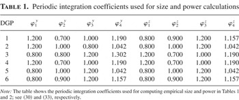
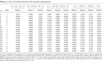
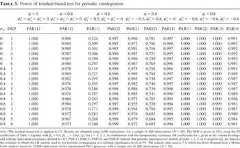
Table 1 shows the combinations of coefficients used in (30)–(33) to compute the empirical size and power. The size and power results are collected in Tables 2 and 3, respectively, for a sample size of 50 years (200 observations) and based on 5,000 replications.

Periodic integration coefficients used for size and power calculations

Size of residual-based test for periodic cointegration

Power of residual-based test for periodic cointegration

The results of Table 2 verify that, even in finite samples, the residual-based test for periodic cointegration has reasonably good size properties, provided that the appropriate order of PAR model is selected. In particular, the order p required in (20) is one greater than the order of the stationary AR component in (31). When a model of too low order is used, the test can be undersized or oversized, depending on the parameters of the process. In general, the satisfactory size (for appropriate p) applies across all sets of PI coefficients considered and irrespective of the extent of correlation between the disturbances. However, the final column suggests that, even for the correct p, the test tends to be undersized with increasing PAR order in the DGP.

Turning to the power results of Table 3, and again provided that an appropriate order of periodic process is fitted, the test has power approaching unity for all cases considered. It is unsurprising that unit power is obtained when the disturbances for y_sτ in (33) are white noise, compared to around 0.98 when these disturbances are a stationary AR(1) with coefficient 0.8. However, power does not diminish substantially when the process contains the root (0.8)⁻¹ = 1.25 together with additional stationary autocorrelation. For example, with stationary AR(4) autocorrelation in a cointegrating PI regression, the test applied to a fitted PAR(4) process has power of at least 0.98 in Table 3. On the other hand, relatively low power is obtained when a PAR(1) is fitted in the context of the stationary AR(2) disturbance process, and to a lesser extent when a PAR(2) is fitted to an AR(3) disturbance DGP. This relatively low power is a consequence of estimating a model of too low order and reflects the undersizing evident in Table 2 for the corresponding cases, which have a (periodic) unit root in place of the stationary root of 1.25.

5.2. Deterministic Terms

To facilitate the preceding theoretical analysis, we omitted deterministic terms and assumed zero initial values, thereby implying E [x_sτ] = 0. Here we relax these restrictions by considering the addition of deterministic terms to the cointegrating test regression.

In the case of standard (nonperiodic) cointegration, the appropriate form of the cointegration test regression depends on the properties of the time series under study; see Phillips and Ouliaris (1990) and Hansen (1992). The inclusion of an intercept allows for possibly nonzero starting values, with means constant over time, by demeaning the variables used in the long-run regression. The null distribution of the LR test for (nonperiodic) cointegration then satisfies (23), with w_m(r) as defined in (19), where it is understood that W^x(r) = [w⁽¹⁾(r),W^z(r)′]′ is a vector of demeaned standard Brownian motions. The addition of a trend allows for a nonzero drift, and the vector of Brownian motions is then demeaned and detrended.

Turning to the case of PI processes, a nonzero starting value in (1) and no deterministic terms imply a seasonally varying mean E [x_sτ] that is constant over years τ = 1,2,…. However, as shown by Paap and Franses (1999), the addition of an intercept to (1) leads to a seasonally varying trend in E [x_sτ] and hence an annual growth rate Δ₄ x_sτ that varies over s = 1,2,3,4. Further, excluding the special case of an I(1) process, they show that a PI process with an intercept cannot have a trend that is common over s = 1,2,3,4, irrespective of whether the intercept is constant over seasons or is seasonally varying. On the other hand, and using a first-order process for ease of exposition, the process

with e_sτ white noise and trend coefficients satisfying

has a common linear trend shared by all quarters (Paap and Franses, 1999). However, with unrestricted trend coefficients, (34) implies seasonally varying quadratic trends in E [x_sτ].

In the context of testing for periodic cointegration, the preceding discussion implies that the relevant cointegrating regressions that may be considered in place of (7) are

and

More specifically, (36) is appropriate when the variables in the regression are known to have constant (possibly periodically varying) mean over time, and the use of (37) permits the possibility that the variables may trend linearly over time.⁸

In addition to the case with unrestricted trends in (37), we also investigate cointegrating regressions using restricted trend coefficients such that β₁₁ = β₁₂ = β₁₃ = β₁₄. This last case is considered when ϑ_s satisfies the restrictions of (35) and hence the linear trend in each PI(1) process is constant over seasons. All DGPs used in this analysis are uncorrelated PI PAR(1) processes.

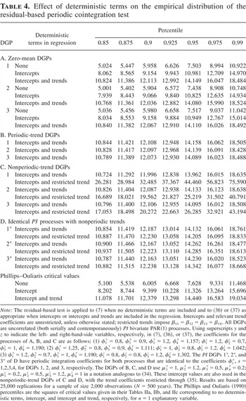
The results of Table 4A verify that, for the three bivariate PI(1) DGPs considered there, the inclusion of deterministic terms has the anticipated effect on the residual-based test for periodic cointegration. That is, for zero-mean processes, the inclusion of periodically varying intercepts or periodically varying intercepts and trends, as in (36) and (37), respectively, causes the distribution of the LR test for periodic cointegration to shift, with the percentiles of the test statistic under the null hypothesis being effectively the same as the corresponding values obtained by Phillips and Ouliaris (1990) for the nonperiodic case (with the latter values squared).

Effect of deterministic terms on the empirical distribution of the residual-based periodic cointegration test

Because the inclusion of unrestricted intercepts leads to seasonally varying trends in a PI(1) process, a cointegrating test regression of the form of (37), with unrestricted intercepts and trends, takes account of these deterministic effects. Table 4B verifies that, in this case, the (squared) Phillips and Ouliaris (1990) critical values for nonperiodic random walks with drifts continue to apply in this periodic case. As seen in Table 4C, these critical values also apply if the individual processes within the DGP have trends restricted to be identical across seasons, provided that no restrictions are imposed when (37) is estimated. However, imposition of the restriction of nonperiodic trends in the cointegrating test regression of (37) causes the Phillips–Ouliaris critical values to be inappropriate for these DGPs.

In contrast to the effects of restricted trends in Table 4C, Table 4D shows that, whether the trend coefficients of the cointegrating test regression are restricted to be identical over seasons or not, the Phillips and Ouliaris (1990) critical values can be used when testing cointegration between two PI(1) processes that have identical periodic coefficients, φ_s^(j) = φ_s,j = y,z. However, the case of identical coefficients across PI separate processes is a special one, for which Lemma 1 shows that any cointegration must be nonperiodic.

To investigate this further, consider the PI(1) vector x_sτ, where all elements have constant trends over seasons. Separating the deterministic and stochastic components of each element, we can write

where ξ_sτ⁽ⁱ⁾ is a zero-mean PI(1) process and E [x_sτ⁽ⁱ⁾] = c_0s⁽ⁱ⁾ + c₁⁽ⁱ⁾τ, which has a periodically varying intercept but nonperiodic trend. The regression relevant for testing periodic cointegration between the zero-mean stochastic unit root processes ξ_sτ⁽ⁱ⁾ is

that is,

which is identical in form to (37). Notice, however, that although (39) has periodically varying intercepts and periodic trend coefficients, the trend coefficients in the latter satisfy

If the PI(1) coefficients are identical across processes, and hence any cointegrating relationship is nonperiodic, then β_i1 = β_i2 = β_i3 = β_i4 (i = 2,…, m), and (40) implies nonperiodic trends in the cointegrating regression of (37) or (39).

The Monte Carlo results of Table 4C and 4D support this analysis. In particular, the PI(1) processes in Table 4D with identical coefficients and individual nonperiodic trends imply that any trend in (37) is also nonperiodic. Therefore, the restriction of identical trends derives from the nonperiodic nature of any cointegration in this case, with the imposition of this restriction effectively having no impact on the distribution of the residual-based test statistic.

On the other hand, when the PI(1) coefficients differ over processes, (40) implies that the imposition of the nonperiodic trend restriction is inappropriate when the β_is are not correspondingly restricted. However, from Lemma 1, nonperiodic cointegration can apply only when the separate processes have identical PI coefficients. Therefore, the trend coefficients in (37) should not be restricted to be nonperiodic when testing for cointegration between periodic processes, except for the special case analyzed in Table 4D.