




No CrossRef data available.
Article contents
- Abstract
- 1. INTRODUCTION
- 2. MODEL CLASS
- 3. DESCRIPTION OF THE ALGORITHM
- 4. ASYMPTOTIC RESULTS IN THE STATIONARY CASE
- 5. ORDER ESTIMATION
- 6. RESULTS IN THE INTEGRATED CASE
- 7. SIMULATIONS
- 8. CONCLUSIONS
- APPENDIX A: RELATIONS BETWEEN ARMAX AND STATE SPACE REPRESENTATIONS
- APPENDIX B: PARAMETERIZATION BASED ON ECHELON OVERLAPPING FORMS
- References
ESTIMATING LINEAR DYNAMICAL SYSTEMS USING SUBSPACE METHODS
Published online by Cambridge University Press: 08 February 2005
Article contents
- Abstract
- 1. INTRODUCTION
- 2. MODEL CLASS
- 3. DESCRIPTION OF THE ALGORITHM
- 4. ASYMPTOTIC RESULTS IN THE STATIONARY CASE
- 5. ORDER ESTIMATION
- 6. RESULTS IN THE INTEGRATED CASE
- 7. SIMULATIONS
- 8. CONCLUSIONS
- APPENDIX A: RELATIONS BETWEEN ARMAX AND STATE SPACE REPRESENTATIONS
- APPENDIX B: PARAMETERIZATION BASED ON ECHELON OVERLAPPING FORMS
- References
Abstract
This paper provides a survey on a class of so-called subspace methods whose main proponent is CCA proposed by Larimore (1983, Proceedings of the 1983 American Control Conference 2). Because they are based on regressions these methods for the estimation of ARMAX systems are attractive as a result of their conceptual simplicity and their numerical advantages as compared to traditional estimators based on criterion optimization. Under the assumption of correct specification the methods provide consistent and asymptotically normal estimates for stationary ARMAX processes where the innovations may be conditionally heteroskedastic and the exogenous inputs are strictly stationary of sufficiently short memory. For stationary autoregressive moving average (ARMA) processes with independent and identically distributed (i.i.d.) Gaussian innovations the estimates are even asymptotically efficient. For I(1) ARMA processes the estimates of both the long-run and the short-run dynamics are consistent without using the knowledge that the data are integrated in the algorithm. Additionally the algorithms provide easily accessible information on the appropriateness of the chosen model complexity. The algorithms include a number of design parameters that have to be set by the user. These include the order of the estimated system. This paper collects up-to-date knowledge on the effects of these design parameters, leading to a number of suggested automated choices to obtain a fully automated estimation procedure.
Information
- Type
- Research Article
- Information
- Copyright
- © 2005 Cambridge University Press
1. INTRODUCTION
Autoregressive moving average (ARMA) and autoregressive moving average with exogenous inputs (ARMAX) systems are traditionally estimated using optimization of some criterion function such as the Gaussian likelihood or related criteria over a set of parametric models. Except in special cases such as ARX models the criterion function is nonlinear in the parameters and does not allow for closed form solutions. Therefore the optimization typically is performed using gradient methods starting from an initial guess. In particular for high-dimensional parameter spaces arising especially for multivariate data sets the optimization is numerically demanding, and local optima are a concern. In these cases the choice of the initial guess is critical. Using suboptimal starting values might lead to a substantial decrease in estimation accuracy. Additionally, for large data sets the gradient search becomes numerically exhaustive and sometimes prohibitive.
Subspace methods on the other hand are based on regressions and hence lead to easily implementable estimators carrying a relatively low computational cost. Moreover, in particular the subspace method called CCA (canonical correlation analysis) has been shown to possess remarkable accuracy properties, being asymptotically efficient in some cases. CCA is known to provide consistent estimators under a variety of conditions, including stationary ARMAX processes. Also for integrated ARMA processes consistency is achieved without using the knowledge of the cointegrating rank. Additionally, order estimation can be performed within the framework of subspace methods at extremely low computational cost. This paper presents the main ideas of subspace methods and reviews the literature on asymptotic results relating to consistency and the asymptotic distribution of the estimated parameters.
Subspace methods can be seen as evolutions of methods based on stochastic realization theory such as the algorithms proposed in Ho and Kalman (1966), Zeiger and McEwen (1974), and Aoki and Havenner (1991). The most popular subspace methods are CCA (canonical correlation analysis, introduced as CVA [canonical variate analysis] proposed in Larimore (1983), N4SID (numerical methods for subspace state space identification, Van Overschee and DeMoor, 1994), and MOESP (multivariate output error state space, Verhaegen, 1994). The main idea of subspace methods is to exploit the structure of the state space representation of ARMAX processes (see Section 2). Given the exogenous input the state summarizes in a certain sense all information of the past that is useful for mean square prediction. The various algorithms use this structure differently. As will be argued in Section 3 the CCA approach seems to be most suited for typical econometric analyses. Hence this survey focuses on this method.
The basic underlying idea of CCA is similar to the so-called Hannan–Rissanen method (sometimes also-called Durbin's method; Durbin 1960), which is discussed in great detail in Chapter 6 of Hannan and Deistler (1988). This method uses preliminary ARX modeling to obtain estimates of the innovations. Using these estimates in place of the lagged true innovations in the ARMAX system equations the ARMAX(p,q,r) system matrices can be estimated by regression for any integers (p,q,r) specifying the maximum lag lengths. Because the state space system equations are linear in the system matrices when the state is known (see Section 2 for details) CCA estimates the state in a first step. Then in a second step the system matrices are estimated using regression in the system equations substituting the estimated state for the true state.
To use CCA a number of design parameters have to be set, resulting in a whole class of algorithms that have been called the state approach to subspace methods. One particular algorithm in this class has been shown to provide system estimators for ARMA processes that have the same asymptotic distribution as the preliminary estimators obtained using the Hannan–Rissanen procedure (see Deistler, Peternell, and Scherrer, 1995, Proposition 4.1). Note that these first step estimators provided by the Hannan–Rissanen procedure are not asymptotically efficient (cf. Hannan and Deistler, 1988, Remark, p. 264), which could be problematic, especially in high-dimensional data sets and in situations where a large number of local extrema are present, and it is hence important to choose the initial guess close to the global optimum. Therefore by optimizing the choices in the state approach the resulting algorithm is not worse than the Hannan–Rissanen procedure. A large portion of the literature on subspace methods in fact focuses on the effects of the various design parameters on the asymptotic distribution of the corresponding parameter estimators. Supplying rules for setting these design parameters then leads to fully automated procedures in the sense that the user only has to supply the data and the algorithm returns an estimated model. It should always be borne in mind that these rules are typically motivated by considerations about asymptotic properties in hypothetical situations that might not be reflected in finite samples in real-world data sets. Thus automated procedures are seen as a starting point for analysis rather than a substitute for research skills.
There are (at least) two shortcomings of this survey. First the paper is focused on a particular method (namely, the state approach) and does not take into account alternative algorithms such as the previously mentioned N4SID and MOESP and different adaptations of CCA such as the algorithms of Peternell, Scherrer, and Deistler (1996). A partial justification for this omission will be provided later. Second this survey neglects a wide range of topics that form a sizable part of the contributions to the engineering literature on subspace methods but do not seem to be relevant for economic data sets. For a related survey including some of these issues see Bauer (2004a).
The paper is organized as follows. In the next section the state space framework is discussed. Section 3 provides a detailed description of the state approach to subspace methods, and Section 4 presents some asymptotic theory for the stationary case under the assumption of correct specification, leading to a number of suggestions for the choice of the design parameters for given order of the system. Section 5 then discusses methods for specification of the order. Section 6 deals with integrated processes. A small simulation study compares subspace methods to pseudo-maximum-likelihood estimation in Section 7. Section 8 concludes the paper. Two Appendixes provide technical details on the relation between state space and ARMAX systems (Appendix A) and the parameterization of state space models based on overlapping echelon forms (Appendix B).
2. MODEL CLASS
In this paper we consider ARMAX processes that are defined as follows: Given a sequence of observed exogenous inputs

and a martingale difference sequence

(for detailed assumptions see Section 4) the process

is an ARMAX process if there exist matrices

and (possibly random) initial conditions yt,t = 1 − p,…,0,zt,t = 1 − r,…,0,εt,t = 1 − q,…,0 such that

solves the vector difference equation (VDE)

for

. The integers p,q,r define the complexity of the model.
Equivalently every ARMAX process

can be written as the solution to the state space equations

for

. Here

are real matrices. The recursions are started using the initial state

, which is assumed to be a random variable with finite second moments uncorrelated with

. The n-dimensional process

is the so-called state process. The state xt is not observed. For explicit expressions of the matrices (A,B,C,D,K) for given ARMAX system see Appendix A, where some relations between ARMAX and state space representations also are provided. A more detailed exposition can be found in Chapters 1 and 2 of Hannan and Deistler (1988). In the following discussion we will deal exclusively with the state space framework. To make the paper accessible for readers unfamiliar with these concepts, the main ideas needed in this paper are discussed in more detail in Appendix A, where the corresponding notions for ARMAX systems also are given for illustration purposes.
The solution to the state space equations is easily seen to be (cf. Hannan and Deistler, 1988, p. 14)

where the last equation defines

. Therefore

denotes the solution to the initial conditions x1 = 0. Denoting K0 := Is,L0 := D,Kj := CAj−1K,Lj := CAj−1B,j > 0 the transfer functions

are both rational functions in

. These equations define the mapping π : (A,B,C,D,K) [map ] (k(z),l(z)) = (Is + zC(In − zA)−1K,D + zC(In − zA)−1B). The transfer functions converge at least for

in a neighborhood of the origin. The state space system (A,B,C,D,K) is called state space representation of the pair (k(z),l(z)) of transfer functions. From (3) it follows that yt can be additively decomposed into

, the solution corresponding to zero initial state, and the effects of a nonzero initial state, i.e., CAt−1x1. From the representation

it is clear that

depends only on the pair (k(z),l(z)) and not on the particular state space representation (A,B,C,D,K) thereof. Thus if the effects of the initial conditions are modeled separately it may be assumed without loss of generality that the system (A,B,C,D,K) is minimal (as defined in Hannan and Deistler, 1988, p. 47; see also Appendix A). For a given pair of transfer functions (k(z),l(z)) a minimal state space representation uses the smallest possible state dimension to represent (k(z),l(z)). The dimension of the state in a minimal state space representation is called the order of the system. The order measures the complexity of the model.
With the exception of Section 6 we will also impose the stability assumption λmax(A) < 1 (where λmax(A) denotes the maximum modulus of the eigenvalues of A), implying that k(z) and l(z) converge absolutely for |z| ≤ 1,

. This implies that for stationary input

the initial state x1 can be chosen such that

is stationary. Furthermore the so-called strict minimum-phase assumption λmax(A − KC) < 1 is imposed throughout, implying that k(z) is stably invertible on |z| ≤ 1. Let Mn denote the set of pairs of rational transfer functions (k(z),l(z)) having a state space representation of order n where (k(0),l(0)) = (Is,0), which are analytic on the closed unit disc and where k(z)−1 is analytic on the closed unit disc. The set of pairs Mn is equipped with the so-called pointwise topology (cf. Hannan and Deistler, 1988, p. 54).
Minimal state space systems are not identified. Changing coordinates in the state space (i.e., using

for nonsingular

as the state) leads to a different state space representation. It is possible to restrict sufficiently many entries of the system matrices (A,B,C,D,K) to zero or one such that the remaining unrestricted entries are identifiable parameters for pairs of transfer functions (k(z),l(z)) in a small enough neighborhood of any given pair (k0(z),l0(z)). In this paper we will use the parameterization based on the overlapping echelon forms described in Section 2.6 of Hannan and Deistler (1988) using such local identification conditions. In the following discussion we will only establish the relevant notation. For details on the construction of these forms see Appendix B. It should also be noted that the parameterization is only introduced as a means to conveniently compare the estimation accuracy of the estimators. Most other results and in particular the description of the algorithms will not use a particular coordinate system for Mn.
The parameterization consists of a finite collection of mappings φα indexed by a multi-index

. For each given α the mapping φα is defined on a subset Mn,α ⊂ Mn such that

attaches the parameter vector θ collecting all free entries to each pair of transfer functions in Mn,α. Theorems 2.6.4 and 2.6.5 of Hannan and Deistler (1988) imply the following properties: The parameter space Θα is an open subset of

for each α. For each multi-index α it holds that Mn,α is open and dense in Mn and φα is continuous on Mn,α. It follows that the specification of α once the order n has been specified is less critical. Finally denoting with

the order of the parameterized pairs of transfer functions, we have ∪α,|α|=n Mn,α = Mn.
From this discussion and Appendix B it is seen that the question of finding a parameterization of ARMAX systems (or for that matter state space systems) for multivariate systems is not trivial. The underlying technical reason is that there does not exist a continuous parameterization for Mn (cf. the discussion in Hannan and Deistler, 1988, Sect. 2.6.). It might seem to be the case that using the maximal lag lengths (p,q,r) as the measure of complexity rather than the system order n simplifies the situation. However, as discussed on p. 77 of Hannan and Deistler (1988), such a parameterization has theoretical disadvantages. Therefore we will use the relatively complicated parameterization given previously. This carries the advantage that for echelon forms the relations between ARMAX and state space parameters are very simple (see Hannan and Deistler, 1988, Theorem 2.6.5, p. 72).
3. DESCRIPTION OF THE ALGORITHM
The basic idea underlying the state approach to subspace algorithms is the fact that if the state were known the state space system equations (2) could be used to obtain estimates of the system matrices using simple regressions. The main problem then is to obtain a good estimate of the state.
In this respect the properties of the state for prediction purposes are central. Consider the problem of predicting yt+j,j ≥ 0 based on the knowledge of

. Let yt+j|t denote the best mean square prediction. Analogous to (3) for j ≥ 0 we have the equation

because

is assumed to be a martingale difference sequence. Note that yt+j|t depends on zl,yl,l < t only via xt and that furthermore yt+j|t is a linear function of the state xt and the future inputs zt+i,i ≥ 0 for all j ≥ 0. On the other hand it follows also from the system equations that
1Here and in the following discussion the integer p does not coincide with the maximal lag length of the ARMAX process used previously.

where for A := A − KC,B := B − KD we have

and Wt,p− := [wt−1′,…,wt−p′]′ denoting with wt the joint process, i.e., wt := [yt′,zt′]′. Therefore it follows that xt is a linear function of the data obtained up to time t and the initial state x1. Under the strict minimum-phase assumption, (A − KC)p will be small for large p, and hence a reasonable approximation of xt is given by

. Therefore an estimate of the state can be obtained by replacing

with an estimate

in this approximation.
These two facts build the basis for the estimation of the state. Consider the prediction equation (4) written jointly for j = 0,…,f − 1 for some integer f (where t > p is assumed):

where Yt,f+ := [yt′,…,yt+f−1′]′ collects the predicted variables, Zt,f+ := [zt′,…,zt+f−1′]′ is the future of the exogenous inputs, and Nt,f+ denotes the prediction errors. Finally

is sometimes called the truncated observability matrix. Expressions for

are easy to derive but not essential for our purposes and hence are omitted.
Equation (5) lies at the core of the subspace idea. Neglecting

under the assumption Ap ≈ 0 the matrices

can be estimated using regression because Wt,p− and Zt,f+ are observed and the residuals Nt,f+ are orthogonal to the regressors. Moreover for f sufficiently large the fact that

, where n denotes the order of the system, can be exploited. This motivates the following procedure.
1. Choose the integers f and p.
2. Estimate the equation Yt,f+ = β1Wt,p− + β2 Zt,f+ + Nt,⊥,t = p + 1,…,T − f + 1 under the restriction rank(β1) = n. This leads to the estimates

of β1 (rank n). In this step also the order n of the estimated system has to be specified.
3. Estimate the state

.
4. Regress yt onto

to obtain estimates

and residuals

.
5. Regress

for t = p + 1,…,T to obtain estimates

to compute the estimates

.
6. Check the minimum-phase assumption. If the estimated system is not minimum-phase the estimated spectrum

where

(and .* denotes conjugate transposition) has to be refactored to ensure that the minimum-phase assumption holds (cf. Hannan and Deistler, 1988, Theorem 1.3.3, p. 26).
The central step in the algorithm is the reduced rank regression. Let

denote the least squares estimator ignoring the rank restriction on β1. Then the rank n approximation

is obtained using the singular value decomposition (SVD)

where

denotes the matrix whose columns are the left singular vectors of

corresponding to the n dominating singular values

denotes the matrix of the corresponding right singular vectors. The approximation error arising from using a system order n is denoted as

. Finally

denote two weighting matrices that for the moment only are assumed to be nonsingular a.s. More specific conditions will be provided subsequently. This results in estimates

. If a different factorization into

for some nonsingular matrix

is used the resulting estimates will be observationally equivalent; i.e., the estimated pair of transfer functions will be unchanged. The asymptotic properties of the state space representation

on the contrary depend on the choice of the factorization.
The term canonical correlation analysis (CCA) has its origin in the approximation step. Let

for two vector sequences

somewhat sloppily using the same symbol for the processes and their realizations at time t. Introduce the notation

such that Yt,f+,Π denotes the residuals of a regression of Yt,f+ onto Zt,f+ and correspondingly Wt,p−,Π are the residuals of the regression of Wt,p− onto Zt,f+ . Then the original version of CCA uses

where X1/2 = (X1/2)′,(X1/2)2 = X denotes the symmetric square root of the positive definite matrix X. Further the unrestricted estimate

. Therefore in the case of no inputs the weightings used in CCA imply that the SVD amounts to the estimation of the canonical correlations and vectors of the two subspaces spanned by the components of Yt,f+ and Wt,p−, respectively (because there is no input here Yt,f+,Π = Yt,f+,Wt,p−,Π = Wt,p−).
The choice of weightings according to (6) corresponds to the maximum-likelihood solution to the reduced rank regression Yt,f+ = β1Wt,p− + β2 Zt,f+ + Nt,⊥ such that rank(β1) = n based on Gaussanity (and uncorrelatedness over time) assumptions on Nt,⊥. The least squares solution is obtained by using

. With respect to

only the choice given previously will be considered throughout. In the following discussion the algorithm using the weightings (6) will be referred to as CCA. Algorithms using a different weighting scheme but the same outline in the literature have been called Larimore approach or state approach. We will use the second term in the following discussion.
In the reduced rank regression both the outputs and the regressors are lags of yt,zt and wt, respectively, and hence the problem has a similar structure as autoregressions. As in autoregressions there are two possible implementations that in the stationary case possess identical asymptotics. Either only time instants are used in the regression where all observations are available, i.e., the range of t is limited to t = p + 1,…,T − f + 1, or alternatively, the regression can be based on the estimated second moments as in the Yule–Walker equations, essentially imposing zero initial and end conditions (cf. Hannan and Deistler, 1988, p. 212). The first approach might seem to be favorable for small sample sizes and relatively large values of f and p as the imposition of zero initial conditions introduces avoidable bias. On the other hand the usage of covariance estimates makes the procedure easily adaptable to data sets including missing values. Using robust estimators of the covariances leads to (statistically) robust versions of the state approach. A recursive (in sample size) formulation of the regression problem leads to recursive estimators.
Finally the term subspace algorithm needs explanation. It originates from the reduced rank regression in the second step as the most popular methods in the class of subspace algorithms, that is, MOESP (Verhaegen, 1994) and N4SID (Van Overschee and DeMoor, 1994), use the matrix

in subsequent steps rather than

. Because the factorization into

is of no importance for the estimated pair of transfer functions, the reduced rank regression problem essentially estimates the subspace spanned by the columns of the matrix

, hence the name. MOESP continues to obtain estimates for (A,B,C,D) but does not estimate K, which implies that only l(z) is estimated. Frequently in econometric analysis one is primarily interested in the noise dynamics, and therefore MOESP does not seem to be a suitable algorithm for these purposes. Therefore it is not considered further in this survey. The same remark is true for one variant of N4SID. An alternative version of N4SID and a recently proposed algorithm by Chiuso and Picci (2003) use a more complicated method to estimate the shifted state

. Because the analysis of these methods is still in its infancy we will not consider these algorithms further. We refer to Chiuso and Picci (2003) for details.
The description of the state approach makes it obvious that there are a couple of design parameters involved. First f and p have to be chosen; second the weighting matrices

and the order n have to be specified. A large part of the literature on subspace methods deals with the effects of these choices on the asymptotic properties of the corresponding estimators. Section 4 will survey the main results in this respect for the stationary case, and Section 6 will deal with the case of integrated processes, whereas Section 5 discusses procedures to estimate the order n.
4. ASYMPTOTIC RESULTS IN THE STATIONARY CASE
Most of the literature on the asymptotic properties of subspace methods deals with the stationary case. Throughout this section we will make the following assumptions on the data generating mechanism.
Assumption 1. The process

is generated by a state space system (2) where the true pair of transfer functions (k0(z),l0(z)) ∈ Mn0,α, i.e., the true order of the system is denoted as n0. Accordingly θ0,α = φα(k0(z),l0(z)) ∈ Θα denotes the true parameter vector which is an interior point of Θα. Thus in particular it is assumed that the system is stable and strictly minimum-phase. The strictly stationary ergodic process

is a martingale difference sequence with respect to the filtration

having the following properties:

Here εt,a denotes the ath component of εt. If no exogenous inputs

are present, the condition on the third moments is not needed.
The input process

has a representation as

where for

it holds that

for some

for some ε > 1 and det kz(z) ≠ 0,|z| ≤ 1. Here the strictly stationary and ergodic innovations process

is independent of

where for the filtration

it holds that

The initial state

.
A couple of remarks on these assumptions seem to be necessary.
- Note that here we use all processes except for
defined on
 rather than onas their time index. This is done for convenience because it allows us to directly use the results for stationary processes in Hannan and Deistler (1988). Because Aj → 0 for j → ∞ at an exponential rate as a result of the stability assumption different choices of the initial state x1 (subject to mild conditions such as finite second moments) do not change any of the results. Similarly restricting the definition of the input tois not critical.
- The assumptions on the innovations sequence are identical to Assumptions AX on p. 131 of Hannan and Deistler (1988) used in proving asymptotic normality for pseudo-maximum-likelihood estimation. For some of the following results these seem to be overly restrictive. In particular consistency results might be expected to hold without the assumption of bounded fourth moments. In the literature no results for weaker assumptions have been reported.
- Note that the innovations sequence is not restricted to be conditionally homoskedastic. Certain autoregressive conditionally heteroskedastic (ARCH) and generalized autoregressive conditionally heteroskedastic (GARCH) processes satisfy the assumptions (cf. the discussion in Bauer, 2004c).
- The input sequence is assumed to be linearily regular excluding typical deterministic terms such as the constant or harmonic terms. This is done to avoid multicollinearity problems in the vectors Wt,p− and Zt,f+ . Rather than including such components as inputs it is suggested that this information be extracted prior to using subspace methods. Analogously to the pseudo-maximum-likelihood case the asymptotic properties of the algorithms applied to the demeaned series are identical to the properties if the true mean is subtracted. Some discussion on this issue may be found in Bauer (2004c).
- Long memory processes such as fractionally integrated processes (see Baillie, 1996) are not admitted as inputs. As we assume that the spectrum of the inputs is nonsingular on the unit circle, differenced long memory processes are also disqualified. This does not imply that subspace methods are not applicable in this setting. To the best of my knowledge this area simply has not been investigated.
The state approach essentially consists of a reduced rank regression used to obtain an estimate of the state and regressions in the system equations (2) to estimate the system matrices. The analysis of the second step is standard, and hence most of the literature focuses on the asymptotic properties of the estimation of the state that are determined by the asymptotics for

. The methods used in the analysis are standard.

is obtained as the right factor of the matrix

estimated in the reduced rank regression. Because regression estimates in a stationary framework essentially are nonlinear functions of the estimated covariances, the asymptotic distribution of

follows using standard linearization techniques of the mapping attaching

to the estimated covariance sequence from the well-documented properties of covariance sequence estimates (under the stated assumptions convergence follows from Theorem 7.4.3 on p. 326 of Hannan and Deistler, 1988; asymptotic normality follows using their Lemma 4.3.4, p. 146). The main technical complications in the analysis are due to the fact that p → ∞ at some rate to make the bias introduced by neglecting the term corresponding to

tend to zero. Another complication is the nonuniqueness of the SVD. Typically

is shown as a first step where

is a matrix of rank n0. Here the dependence of the SVD on the integers f and p is made explicit. However, the SVD written as Un0(f,p)Σn0(f,p)Vn0(f,p)′ is not unique where

contains the singular values. Even in the case where the singular values σ1(f,p) > σ2(f,p) > ··· > σn0(f,p) > 0 are distinct the singular vectors (being the columns of Un0(f,p) and Vn0(f,p)) are only unique up to the orientation. If (ui,vi) denotes the pair of left and right singular vectors corresponding to σi(f,p) then (−ui,−vi) is another such pair. Therefore it is necessary to impose additional conditions on the SVD to achieve uniqueness and subsequently continuity and differentiability of the factorization of

into

(for a detailed discussion see Bauer, Deistler, and Scherrer, 1999, p. 1246, bottom right column). In cases of repeated singular values the situation is more complicated.
As noted previously the choice of the factorization of

is not essential for the estimated pair of transfer functions. Any factorization will lead to the same estimate

. The main differences lie in the asymptotic properties of the corresponding estimated system

. For consistency of

the existence of one factorization such that the corresponding system estimate

converges is sufficient. There are factorizations that simplify the mapping attaching

to the estimated covariance sequence significantly (for details in the case of no inputs see Bauer, 2004c, Lemma 3, and the references given therein).
Using these techniques consistency for the transfer function estimators obtained via the state approach under various different assumptions has been established in a number of papers. Deistler et al. (1995, Proposition 3.2) prove consistency for the transfer function estimates obtained by CCA in the case of no inputs under Assumption 1 and the additional assumptions that

for some d > 1. Here [lfloor ]x[rfloor ] denotes the integer part of the real

denotes the optimal lag length for an autoregressive approximation of yt selected by minimizing the BIC over 0 ≤ p ≤ (log T)a for some constant 0 < a < ∞. Peternell et al. (1996, Theorem 3.1) extend these results by including ARMA inputs such that the innovations of the joint process wt form a conditionally homoskedastic martingale difference sequence with bounded unconditional fourth moments and

(their algorithm uCCA) or

, respectively (their algorithm N4SID).
2There the restriction D = 0 also is imposed. It is obvious that this is not essential for the result.

follows along the lines of Theorem 1 in Bauer (2004c). A detailed proof of the following statement is contained in a preliminary version of this paper and can be obtained from the author on request.
Sufficient Conditions for Consistency. Let the process

and the input process

fulfill Assumption 1. Suppose that n0 is known and used in the state approach. Assume that either

is used in the estimation and that either f ≥ n0 fixed independent of the sample size or f = p is used where p → ∞ a.s., p = o((log T)a) for some a < ∞. Then

a.s.
Some of these conditions clearly are not necessary. If f is kept fixed then the weighting matrix

can be chosen arbitrarily such that

a.s. Also f = p might seem to be too restrictive, and other conditions could be derived. Further the upper bound on the increase of p seems to be too conservative, and it seems likely that less restrictive upper bounds of the form p = o(Tδ) for some δ > 0 might be sufficient. It should be noted that the assumptions given previously also include the case that f and p are chosen depending on the data such as the choice

. Almost surely convergence to infinity of p subject to the upper bound (log T)a is sufficient in this respect. For example any choice of

satisfies these bounds for 0 < ρ0 = λmax(A − KC) < 1 by Theorem 6.6.3 of Hannan and Deistler (1988, p. 261) stating that

a.s. Alternatively

could be used in the definition of f and p.
Note that

implies that

a.s. for large enough sample size T. Therefore

is defined a.s. for large enough T. In order to complete the definition of

we assign an arbitrary parameter vector θc, say, to pairs

. Then

a.s. holds as a result of the continuity of φα.
The sufficient conditions given here are too weak to obtain the usual square root sample size rate of convergence. Such a rate is required for the derivation of the asymptotic distribution. It has been noted in Theorem 1 of Bauer (2004c) in the case of no inputs that in addition to the sufficient conditions given previously p ≥ −d log T/(2 log ρ0),0 < ρ0 = λmax(A − KC) < 1,d > 1,p = O((log T)a) is sufficient for

the rate of the law of the iterated logarithm (LIL). The case ρ0 = 0 corresponds to the special case of ARX systems, which will not be dealt with here. In the following it will always be assumed that ρ0 > 0. For exogenous inputs fulfilling Assumption 1 it can be shown that p ≥ −d log T/(2 log ρ0),p = O((log T)a),d > 1 is sufficient for

.
3A proof of this statement is contained in a preliminary version of this paper, which can be obtained from the author on request.
Sufficient Conditions for Asymptotic Normality. Let the process

and the input process

fulfill Assumption 1. Suppose that n0 and α are known and used in the state approach. Assume that either

is used in the estimation. Then if f ≥ n0 is fixed independent of the sample size and the data and p ≥ −d log T/(2 log ρ0), 0 < ρ0 = λmax(A − KC) < 1, p = O((log T)a) for some a < ∞, d > 1 where p is chosen deterministically we have that

converges in distribution to a normal random variable with mean zero. If no exogenous inputs are present the same holds true for f = p under the assumptions on p given previously.
Asymptotic normality results under Assumption 1 in the case of no inputs and conditionally homoskedastic innovations have been obtained in Bauer et al. (1999, Theorem 1) and extended to ARMA inputs such that the joint process wt has conditionally homoskedastic innovations in Bauer (1998). See Theorem 4.3.1 (f fixed) and Theorem 4.3.2 (f → ∞). All three results consider only the case where the true system lies in the subset Mn0+ ⊂ Mn0 characterized by the fact that limT→∞ mini=1,…,n0−1[σi(f,p) − σi+1(f,p)] > 0 (where the assumptions ensure that the limit exists). Hence in Mn0+ asymptotically the singular values are distinct. Bauer (2004c, Theorem 2) extends these results in the case of no inputs to the statement given in the sufficient conditions. The proof of the general result for f ≥ n0 as stated earlier is contained in a preliminary version of this paper and can be obtained on request. The proof for f → ∞ in the no inputs case is analogous to the proof in Bauer et al. (1999) using the result of Bauer, Deistler, and Scherrer (2000).
Note that p ≥ −d log T/(2 log ρ0) ensures that (A − KC)p = o(T−1/2). This condition is the analogue of conditions typically used in the analysis of autoregressive approximations (cf. Lewis and Reinsel, 1985, Theorem 2(iii)) and ensures that the asymptotic mean of

is zero. It has been advocated in Deistler et al. (1995, p. 1866) to choose

for some d > 1 where again

denotes the lag length of an autoregressive approximation of yt of the ARX type selected by minimizing the BIC over 0 ≤ p ≤ (log T)a. The choice of the constant d is an open question. It should also be noted that the choice

is not covered by the sufficient conditions for asymptotic normality given previously because it depends on the data. Asymptotic normality results for stochastic choices of f and p have not been derived in the literature. In the autoregressive setting asymptotic normality of the estimated autoregressive coefficients for data dependent lag length has been obtained recently by Kuersteiner (2005). It seems likely that similar techniques also can be used to prove the asymptotic normality of

for the suggested stochastic choices of f and p. This is an open point in the literature with serious consequences for the validity of the arguments to follow.
In this respect also note that the relation between CCA and autoregressive approximations is very close. Dahlen and Scherrer (2004) show that in the case of no inputs for f = p the CCA estimates essentially are obtained via model reduction based on a preliminary autoregressive approximation.
In the general case no interpretable expression for the asymptotic variance, i.e., the variance of the limiting normal variable, is known. This implies that the effects of the various design parameters on the asymptotic distribution in the general case are unknown. The sufficient conditions only lead to upper and lower bounds on the increase of p as a function of the sample size. Bauer et al. (2000) show that in the situation of Bauer et al. (1999) (i.e.,

the choice of the weighting

does not influence the asymptotic distribution if there exists a sequence of deterministic matrices Ξp− such that

a.s. for some ε > 0. These conditions hold for all choices of

proposed in the literature.
It follows from the proof of Lemma 3 in Bauer (2004c) that the results of Bauer et al. (2000) rely only on the uniform boundedness and convergence (both with respect to the two norm) of the weighting matrices and the convergence of

in the Frobenius norm. Hence the independence of the limiting distribution from the weighting

(subject to the previously mentioned conditions) is easily extended to the general case. Therefore only one choice of

is contained in this paper.
To obtain simple expressions for the asymptotic variance in addition to the sufficient conditions for asymptotic normality given earlier assume that the input is a martingale difference sequence; in particular it is assumed that Kz,j = 0, j > 0. The innovations εt are assumed to be conditionally homoskedastic, i.e.,

. Further assume that (k0(z),l0(z)) ∈ Mn0 is contained in a generic subset Mn0i of Mn0 characterized by the fact that the matrix of the first n0 columns of

is nonsingular (for discussion see Bauer, 2004c, Lemma 3). Using a parameterization of Mn0i based on the unique state space representation for which the matrix of the first n0 columns of

equals the identity matrix Bauer and Ljung (2002) provide a rather explicit expression for the variance of the normal limit of the (appropriately scaled) estimation error for the parameter vectors.
4To be precise: There

is assumed to be i.i.d., where it is remarked that the result also holds in the martingale difference framework considered in this paper.

is differentiable on Mn0i ∩ Mn0,α. Then the Delta method can be used to derive the corresponding expression for the asymptotic variance of

. Thus if

denotes as previously the state approach estimate obtained using

such that

for some deterministic matrix Ξf+ > 0 and ε > 0 and f ≥ n0 fixed and finite we have that

converges in distribution to a normal random variable with mean zero and variance Vf of the form

Here

are matrices that depend on (k0(z),l0(z)) and on

but not on

. Further

. Explicit expressions for M1 and M2 can be derived from the proof of Theorem 1 in Bauer and Ljung (2002). The central term here is

where

. The design parameters

influence Vf only via

. Corollary 2 of Bauer and Ljung (2002) shows that for each f the minimum of Vf is achieved using Ξf+ = limT→∞〈Yt,f+,Π,Yt,f+,Π〉−1/2. Given the identity of the asymptotic distribution of the estimators obtained in the first step in the Hannan–Rissanen procedure with subspace estimators using a particular choice of

(Deistler et al., 1995, Proposition 4.1) it follows that the estimates obtained using CCA improve upon the Hannan–Rissanen estimates in the case of no inputs. Moreover, the minimum value is monotonically decreasing in f. Therefore in the case of no exogenous inputs or white exogenous inputs and conditional homoskedasticity f should be chosen large, and the CCA choice for the weighting matrices should be used under the assumption of specifying the true order in the estimation.
Further specializing, consider the situation of no inputs. Then using f = p ≥ −d log T/(2 log ρ0),p = o((log T)a) for some d > 1 the CCA estimate

is asymptotically equivalent to the pseudo-maximum-likelihood estimate

maximizing the pseudo-likelihood based on Gaussianity and independence of

over Θα. Here equivalence means that

. For conditionally homoskedastic innovations this is shown in Bauer (2000). Hence if no inputs are present and the innovations are independent and identically Gaussian distributed CCA for f = p is not only optimal among the state approach subspace algorithms but in fact efficient. In other words, in this case one does not pay a price in terms of asymptotic accuracy for the numerical advantages. Bauer (2004c) extends the result that

to the conditionally heteroskedastic case (i.e., under the assumption on εt stated in Assumption 1). This implies that for conditionally heteroskedastic or non-Gaussian innovation processes CCA does not achieve the optimal accuracy and its asymptotic properties are analogous to the asymptotic properties of the pseudo-maximum-likelihood estimator ignoring the conditional heteroskedasticity.
In the case of general colored exogenous input process

examples have been found where CCA does not achieve optimal performance (for an example, see Bauer and Jansson, 2000). This lack of optimality has been the motivation for the proposal of slightly modified versions of CCA in Peternell et al. (1996). Although these algorithms decrease the asymptotic variance in some cases (see the calculations of the asymptotic variance in Bauer, 1998, p. 131) no analytical results are known comparing the asymptotic distributions of the basic CCA algorithms and these refined methods in general.
All results up to now relate to the case of correctly specified order n0. In fact few results have been obtained up to now in misspecified cases. For fixed f under the assumptions given in the sufficient conditions for consistency

converges to zero. Let

denote the matrix of left singular vectors corresponding to the dominating

eigenvalues of

. Then the space spanned by the columns of

converges in the gap metric for

(for a definition of the gap metric see Chatelin, 1983, p. 86). Consequently it can be shown that for

the subspace estimators

using order

(fixed and deterministic) converge a.s. to an approximating system

that in some cases can be explicitly given (for details see Bauer, 1998, Sect. 5.3.2). However, nothing is known about the properties of the approximating system.
5. ORDER ESTIMATION
Up to now it was always assumed that the true order of the system is known. This section will discuss methods to specify the order.
The first step in the subspace procedure is a reduced rank regression in the equation

under the constraint rank(β1) = n. The first idea for order estimation hence would be to use the reduced rank regression framework. Under the assumption that Nt,⊥ is i.i.d. Gaussian the likelihood ratio between using rank(β1) = n and rank(β1) = n + 1 is equal to

where

denotes the ith largest singular value of 〈Yt,f+,Π,Yt,f+,Π〉−1/2〈Yt,f+,Π,Wt,p−,Π〉〈Wt,p−,Π,Wt,p−,Π〉−1/2 (Anderson, 1951). But

where

Therefore (Nt,⊥)t=p+1,…,T−f+1 is not uncorrelated over time and moreover depends on p. Consequently the distribution of the pseudo-likelihood ratio does not follow from standard theory. To the best of my knowledge the asymptotic distribution of the likelihood ratio is not known.
An alternative idea then is to formally use the information criteria defined as

where

denotes the number of nonzero singular values. Here d(n) = 2sn + sm + nm equals the number of parameters included in a model of order n and CT > 0,CT /T → 0 denotes the penalty term punishing complex models. Here SVC stands for singular value criterion. It should be stressed that this criterion is not an information criterion being defined in a misspecified case for the same reasons that the likelihood ratio does not follow standard asymptotics. This criterion has been discussed by Camba-Mendez and Kapetanios (2001). Peternell (1995) introduced a similar criterion using

, the Frobenius norm of the approximation error. Bauer (2000) proposes

, i.e., the two norm of the approximation error, based on simulations. The advantage of the last two criteria is that they can be used for general weighting matrices

, whereas the first criterion uses the CCA choices to guarantee

. In the following discussion we will only deal with these three choices.
The order is estimated as the minimizing integer of SVC(n;CT) resulting in an estimator

. The rationale behind these estimates is that

where the matrix Un0(f,p)Σn0(f,p) × Vn0(f,p)′ contains at most n0 nonzero singular values, the remaining ones being zero. Recall that it is the rank of β1 that we want to infer from the noisy estimate

. Letting the penalty factor CT > 0 tend to infinity such that CT /T converges more slowly to zero than the maximal estimation error in the singular values then ensures that asymptotically the penalty dominates and asymptotically the order is not overestimated, implying that
5Here f and p are functions of the sample size T, which is not emphasized in the notation.

. In fact we have the following condition.
Convergence of Order Estimation Using SVC(n;CT). Let the processes

fulfill Assumption 1 with homoskedastic innovations

where the true order is denoted as n0. Additionally it is assumed that for some constants 0 < c < ∞ and 0 < ρ < 1 it holds that

. Assume that f and p are either fixed and finite or tend to infinity, in which case f ≤ p,p = O((log T)a),a < ∞ is assumed. Let Un0(∞)Σn0(∞)Vn0(∞)′ denote the limit of

, which for f → ∞ or p → ∞ (a.s.) has to be interpreted in an appropriate sense (for details see Bauer, 2000). Then CT > 0,CT /T → 0,CT /(fp log log T) → ∞ is sufficient for

to converge to rank(Un0(∞)Σn0(∞)Vn0(∞)′).
Note that Un0(∞)Σn0(∞)Vn0(∞)′ depends on the choice of f and p. Jansson and Wahlberg (1998) show by example that f ≥ n0 + 1,p ≥ n0 is not sufficient for σn0(f,p) > 0. However, violation of this condition is rare because Bauer and Jansson (2000) show that for fixed pseudostationary input sequence

that is persistently exciting of order f + p − 1 (i.e., fulfilling conditions (4.1.1.), (4.1.14), and (4.2.21) of Hannan and Deistler, 1988, the latter with f + p − 1 inserted for sp; these assumptions hold for a particular realization of a process

fulfilling Assumption 1) for fixed f and p the subset of pairs of transfer functions in Mn0 with σn0(f,p) = 0 is the complement of an open and dense subset. This implies that for any given f,p it is unlikely that the true system happens to have the property σn0(f,p) = 0. Nevertheless the problem is relevant because for systems close (in an appropriate sense) to these exceptional systems the smallest singular value will be very small and hence a large number of observations will be needed to differentiate these singular values from noise. Chui (1997) gives sharp conditions on f and p for n0 = rank(Un0(f,p) × Σn0(f,p)Vn0(f,p)′) that imply the sufficient conditions min(f,p) ≥ 3n0. Another set of sufficient conditions is f ≥ n0 and p → ∞.
Bauer (2001, Theorem 3) states consistency of order estimation using SVC(n;CT) for p → ∞ under the assumptions on the input given previously. Only the Frobenius norm and the two norm of

in the definition of SVC(n;CT) are considered in that paper. There convergence of

for fixed and finite f and p also is discussed (allowing a harmonic process to be added to the process fulfilling the assumptions just stated). Because again mainly the uniform convergence of the sample covariances is used in the proof of Theorem 3 of Bauer (2001) the consistency proof for SVC(n;CT)-based order estimation given there can be straightforwardly generalized to yield the result given earlier.
6A full proof of this fact is contained in a preliminary version of this paper and can be obtained on request.

. In this case the condition CT /(fp log log T) → ∞ has to hold a.s. Again the sufficient conditions are by no means necessary.
Simulation evidence shows that for

the sufficient condition on the penalty term seems to be too pessimistic, leading to a high risk of underestimating the order in finite samples (see the simulations in Bauer, 2001). The criterion based on the two norm seems to be less sensitive with respect to the choice of f and p than the method based on the Frobenius norm. No thorough motivation for any penalty term has been found.
A second approach to the problem of order specification is to note that the problem of selecting the order is equivalent to inferring the rank of the noisy matrix

. Different procedures using sequential testing are developed in Sorelius (1999) in the case of no exogenous inputs included (m = 0) and Camba-Mendez and Kapetanios (2001). All these procedures center on the assessment of the rank of 〈Yt,f+,Wt,f−〉 and proceed by sequentially testing for singularity of the matrix and increasing the size by one in case of a rejection until the test is not rejected for the first time.
The Hankel structure of the matrix 〈Yt,f+,Wt,f−〉 complicates the derivation of the test statistic considerably. Additionally one runs into a sequential testing problem. Having said that, it should also be mentioned that this approach is statistically much sounder than the ad hoc definition of criteria such as SVC(n;CT). At present the development of this strand of literature is deemed to be premature, however. We will not go into detail in this respect, and we refer the reader to Sorelius (1999) and Camba-Mendez and Kapetanios (2001) for details.
A third approach to order estimation uses analogies to traditional information criteria. In the context of pseudo-maximum-likelihood estimation the order is estimated using information criteria such as the Akaike information criterion (AIC) or BIC (for details see Hannan and Deistler, 1988, Ch. 5). Assume that the Gaussian likelihood is maximized over Mn for n = 0,1,2,…,HT for some upper bound HT such as (log T)a, 0 < a < ∞, resulting in an estimate

for each n. Then an estimate of the one step ahead prediction errors

is obtained from Kalman filtering (for details see Hannan and Deistler, 1988, Ch. 3), leading to an estimated one step ahead prediction variance

. Then the information criterion estimate is taken as a minimizing integer of the criterion

where again d(n) = 2sn + sm + nm denotes the number of parameters included in a model of order n and CT > 0, CT /T → 0 denotes the penalty term punishing complex models. BIC uses CT = log T and AIC uses CT = 2.
For subspace methods there are two obvious generalizations of this approach. The pseudo-maximum-likelihood estimator

could simply be replaced by the subspace estimator

in the definition of

. Alternatively the estimation of the equation

immediately leads to an estimate of the residual variance

that can be inserted into

. Here the dependence of

on the usage of the n-dimensional state

is emphasized. These two alternatives are fundamentally different. Whereas

takes the full system dynamics into account,

is calculated on the basis of the n-dimensional estimated state, which in the limit need not correspond to an n-dimensional system.
To illustrate the point assume for the moment that we are selecting the model order based on the knowledge of the true state

corresponding to a state space representation such that C = [Is,0] where n0 > s is assumed. Then let xt(n),1 ≤ n ≤ n0 denote the vector of the first n components of xt. Now order estimation based on

, i.e., the residual variance of the equation

, will result in an order estimator converging to s (for suitable choice of the penalty term CT) because the remaining coordinates of xt do not contribute to the prediction of yt. The order estimate based on

, however, will lead to consistent order estimates because in this case for each order n a new estimate of the state also is obtained from the Kalman filter, which for n < n0 will not coincide with xt(n).
For the subspace methods the estimated state

may not correspond to a true system where the last columns of C are zero for any pair (k0(z),l0(z)) because the limiting system is determined implicitly in the SVD. But problems for the order estimation procedure are expected also in situations where the norm of the last column is small. An example in this respect is provided in Bauer (2001), where some asymptotic properties of the order estimate obtained by minimizing

also are derived. Here IVC stands for innovation variance criterion. Because of these problems the use of the criterion is strongly discouraged.
Finally in this section the asymptotic properties of the order selection based on

where

denotes the CCA estimator using f = p,p ≥ −d log T/(2 log ρ0), d > 1,p = O((log T)a),p chosen deterministically, are investigated. Additionally assume that

so that no inputs are included. In this case it can be shown that

and therefore CT > 0,CT /T → 0,CT /log log T → ∞ is sufficient for weak consistency of the order estimate obtained by minimizing

over 0 ≤ n ≤ ps. The expression for n ≠ n0 is immediate because

minimizes

. For n = n0 the expression is a consequence of

. The details of the proof are omitted.
In the situation without inputs zt the criterion

has the tremendous advantage compared to

that once the state has been estimated for a maximal order the subspace estimators for a range of different orders can be obtained extremely numerically efficiently (in fact, only one regression has to be estimated; for details, see Bauer, 2001, p. 1564). Therefore, Kalman filtering to obtain

constitutes the only main computational cost. This idea also has another interesting feature. As stated in Section 4, CCA produces asymptotically optimal estimators in the correctly specified case for Gaussian innovations. For misspecified cases no such result is known, and therefore the subspace estimator might result in worse values of the criterion function than the pseudo-maximum-likelihood estimator that minimizes

. Hence order estimation based on

could be expected to improve on BIC order estimation. It should be stressed, however, that the performance in cases where there exists a true model might not be the only criterion to assess the quality of a model selection procedure (cf. the discussion in Shibata, 1981).
6. RESULTS IN THE INTEGRATED CASE
Because the state approach is primarily based on regressions it seems to be tempting also to apply the algorithm to integrated processes. The assumptions in this section will be as follows.
Assumption 2. The process

is generated by a minimal state space system (2) of order n0 of the form

where

, and c ≤ s and the remaining matrices are of conformable size. Here m = 0, and hence no exogenous input is present. The initial state x1 is assumed to be chosen according to

. Here λmax(A[bull ]) < 1 and 0 < ρ0 = λmax(A − KC) < 1 is assumed. The strictly stationary ergodic noise

is a martingale difference sequence with respect to the filtration

such that

where εt,i denotes the ith component of the vector εt.
As a consequence of the specific structure of the state space system

follows. This basically amounts to a partial fraction decomposition of k0(z) := Is + zC(In − zA)−1K. Using (3) it follows that


Choosing

it follows that

. Hence there exist initial conditions y0 such that

is stationary and also

is stationary for each

. Therefore

is I(1) and admits s − c cointegrating relations because minimality implies that C1 is of full column rank and K1 of full row rank (see Bauer and Wagner, 2002b, Theorem 1). The cointegrating space equals the orthogonal complement of the column space of C1. Restricting x1 to be as in Assumption 2 is no severe loss of generality. All results to follow continue to hold for random x1 with finite second moment and independent of

.
Assume that CCA using f ≥ n0 fixed and finite independent of the sample size is used to estimate the transfer function

. Here n0 denotes the true order, which is assumed to be known and used in the estimation. Let p be chosen deterministically such that p = o((log T)a) for some arbitrary a < ∞ and p ≥ −d log T/(2 log ρ0),d > 2. Then for

generated according to Assumption 2 the following statements hold.
1.

a.s. (Bauer, 2004b, Theorem 3.1). The transfer function—and hence the long-run and short-run dynamics—is estimated consistently without using the knowledge that

is integrated in the algorithm.
2.

in probability for i = 1,…,c for any γ < 1 where

denote the c dominant singular values of

(Bauer and Wagner, 2002a, Theorem 4).
7Unfortunately there is an error in that theorem. The given asymptotic distribution is incorrect; the order of convergence is correct, however.
3. If

where SVC uses

then

in probability for CT > 0,CT /T → 0,CT /(p log log T) → ∞ (see Bauer and Wagner, 2002a, Theorem 3).
4. If

, denote the eigenvalues of

ordered decreasing in modulus then the asymptotic distribution of

is identical to the asymptotic distribution of the vector of the c eigenvalues (ordered decreasing in modulus) of

where

is i.i.d. standard normally distributed and

(Bauer, 2004b, Theorem 4.1). This implies that the largest (in modulus) eigenvalues of the estimated matrix

can be used to test for the number of common trends. The resulting test statistic is pivotal and the asymptotic distribution standard in unit root tests.
Although the transfer function estimator is consistent according to statement 1 the (untransformed) estimators for the system matrices will diverge if the state is estimated as

because this implies

. Therefore the nonstationary state components are downweighed and the corresponding columns in

are multiplied by

. Of course, if the system matrix estimates are transformed into an echelon overlapping form the system matrix estimators also will be consistent.
Note that as a result of consistency the c largest eigenvalues of

will be close to one albeit different without investing the knowledge of c in the algorithm. If knowledge of c is used in the algorithm a reduced rank regression in the equation

subject to

ensures that

corresponds a.s. to an estimated system having a representation as in Assumption 2.
Consistency ensures that CCA can be used to obtain an initial guess for subsequent pseudo-maximum-likelihood estimation. Moreover CCA provides easily accessible information on the model order (via the estimated singular values) and the number of common trends (via the eigenvalues of the matrix

. This information can be used to specify the model prior to the application of pseudo-maximum-likelihood estimation.
The topic of the estimation of unit root processes using subspace methods really is only in its infancy. Although Bauer (2004b) derives the asymptotic distribution of the subspace estimators, this does not reveal much information. In particular no comparison to pseudo-maximum-likelihood estimators has been achieved so far.
There is a subtle difference in the choice of p for the integrated case as opposed to the stationary case that seems worth mentioning: In the stationary case it has been argued that

is a reasonable choice. In the integrated case, however, d > 2 is imposed in the sufficient conditions given previously. The reason for this change is simple: d > 1 ensures that (A − KC)p = o(T−1/2), which is sufficient in the stationary case to ensure that the term

does not influence the asymptotic distribution. In the integrated case on the contrary the convergence in some components of the system matrices is of order OP(T−1), and therefore d > 2 is imposed, leading to (A − KC)p = o(T−1).
7. SIMULATIONS
It has been argued that the main advantage of subspace identification lies in the numerical simplicity and reliability as an initial guess. These claims have been confirmed in a number of simulation studies. The statistical properties of CCA have been highlighted by Peternell (1995), Deistler et al. (1995), Peternell et al. (1996), and Bauer (1998). Bauer (2004c) also contains a comparison of the numerical load. In the integrated case Bauer and Wagner (2002a) demonstrate the usage of CCA for estimating the cointegrating rank, and Wagner (2004) examines the finite sample properties of the estimation of the cointegrating space and the predictions based on the CCA estimates. In this section a small simulation study will be used to demonstrate the claims of the paper. The simulation is not intended to mirror any particular application, and the simulated systems are totally arbitrary. The results reflect the findings in the literature and therefore can be seen to be typical. The main point to be made in the simulations, however, is that there are situations in which subspace methods appear to be a useful alternative to the classical estimation methods.
In the simulation experiment CCA is compared to the algorithm PEM of the MATLAB system identification toolbox. This routine uses an initial estimate obtained by a version of N4SID to afterward maximize the Gaussian likelihood in a Gauss–Newton type method. The method has been chosen because of its widespread use in the engineering community. The basic setup is the following: For each experiment three integers (s,n,T) are given where s denotes the output dimension, n the system order, and T the sample size. Based on these integers an ARMA system is drawn randomly and 100 time series of dimension s and sample size T + 1,000 are generated using this one system and Gaussian white noise of zero mean and variance equal to the identity matrix. The initial conditions are set to zero, which might be seen as unrealistic. Then CCA setting

and estimating the order via SVC(n;log T) based on the two norm

is used to estimate the system on the first T data points. After the completion of this estimation another system is estimated on the same data set using the function PEM and the order estimated in CCA. For both estimated systems the one step ahead prediction error on the remaining 1,000 time instants is calculated. As a measure of accuracy

is chosen where

denotes the estimated innovation variance on the validation sample for the two procedures. For the true system

asymptotically is normally distributed with mean zero and variance 2s. For each experiment three numbers are reported for each of the two algorithms.
1. The average time spent on the algorithm as estimated from the MATLAB function profile.
2. The average of the 100 accuracy measures

where i = 1 for CCA and i = 2 for PEM.
3. The average over the subsample where PEM is not obviously trapped in a local minimum: In some cases the estimation error for PEM is many orders of magnitude too high compared to the error attained by CCA. Formally these cases are defined somewhat arbitrarily by

.
These three numbers are reported for each setting of integers (s,n,T) in Table 1. The main findings are shown.
- CCA is always numerically cheaper than PEM. The difference becomes remarkable for large sample sizes and high-dimensional data sets.
- The specification of the initial guess is an issue. If one does not account for local optima the performance of PEM is worse than the performance of CCA in most cases.
- In medium sample sizes (here T = 1,000) PEM achieves slightly better performance.
- For large sample size PEM does not seem to be trapped in local optima. At the same time the performance is not differentiable from the performance of CCA.
- For small sample sizes SVC picks overly small orders. This is especially the case for high-dimensional data sets. The consequence is a sizable bias.
These findings demonstrate the claims based on asymptotic theory raised in the literature.
Numerical and statistical properties of CCA and PEM

8. CONCLUSIONS
The main advantage of CCA and subspace methods in general in comparison to conventional estimation methods based on criterion minimization is the computational burden. Because it is based on regressions rather than nonlinear optimization, CCA can be applied in situations where pseudo-maximum-likelihood methods are infeasible. Three such situations are data sets with many inputs/outputs, very large data sets, and input selection problems that require a huge number of models to be estimated. In these cases the computational load is one of the prime issues, and hence subspace methods are a valuable alternative to classical estimation methods.
In other cases CCA may be used to obtain initial guesses that are not worse then traditional methods such as the Hannan–Rissanen method. Additionally, in a regression framework issues such as outliers, missing observations, and recursive estimation are well understood. This provides the basis for simple adaptations of the CCA idea.
When using CCA a number of design parameters have to be set by the user. Only in the case of no or white inputs does the literature provide guidance on how to choose these parameters optimally (with respect to the asymptotic variance). Based on these results (albeit not fully justified) CCA using

and the weightings (6) is proposed. Combining this choice with order estimation using SVC(n;CT) and testing for possible integration one obtains an automated procedure in the sense that the algorithm estimates a model given only the data without any additional interaction with the user. As indicated in the Introduction such automatic procedures should be used with caution. Bauer and de Waele (2003) show that such a procedure works well in some examples but fails to exhibit the expected properties based on the asymptotic theory in other situations. A weak point in the algorithm as stated earlier is the simplistic order estimation, which might cause the observed deficiency. Nevertheless at the very least the subspace estimators provide in many cases good starting points for consecutive analyses.
A very attractive feature of CCA is the demonstrated robustness with respect to the data characteristics inherited from the regression framework. It has been stated previously that key properties such as consistency of the transfer function estimates and system order estimates are robust with respect to conditional heteroskedasticity of the innovations or certain nonstationarities of the data. We therefore consider CCA an interesting addition to the toolbox of time series analysts.
APPENDIX A: RELATIONS BETWEEN ARMAX AND STATE SPACE REPRESENTATIONS
The properties of the stochastic processes

being the solutions to VDEs (1) are well understood (for a detailed discussion see, e.g., Hannan and Deistler, 1988, Chs. 1 and 2). Typically the ARMAX system is described using three matrix polynomials (in

) a(z) := Is + A1 z + ··· + Ap zp,b(z) := Is + B1 z + ··· + Bq zq,d(z) := D0 + D1 z + ··· + Dr zr and the initial conditions for yt,zt,εt. Given the noise

, the input

, and the system (a(z),b(z),d(z)) each set of initial conditions determines a unique solution process

. Holding everything else fixed the difference vt := yt1 − yt2 between two such solutions

for different initial conditions is a solution to the homogenous equation

The matrix polynomials (a(z),b(z),d(z)) are called ARMAX representation of the pair of rational transfer functions

that converge at least for

in a neighborhood of the origin. Let

. It follows that

is the solution to the VDE(1) with zero initial conditions and any solution

to the VDE(1) can be written as

where

solves the homogenous equation (8). Note that

depends on the pair of transfer functions (k(z),l(z)) but not on the particular representation (a(z),b(z),d(z)). In other words except for initial effects the pair of transfer functions (k(z),l(z)) fully specifies the input/output behavior of ARMAX systems.
Following p. 15 of Hannan and Deistler (1988) for an ARMAX process

define the state vector

and the matrices

where empty positions contain zeros. Then it is straightforward to check that

solves the corresponding state space equations, i.e., yt = Cxt + Dzt + εt where xt+1 = Axt + Bzt + Kεt. For AR processes the matrix A thus obtained is called the companion form of the polynomial a(z).
On the other hand (3) decomposes a state space process into a component

depending only on the pair of transfer functions (k(z),l(z)) and the effects of the initial conditions CAt−1x1. The use of the same symbol

for the solutions to zero initial conditions for ARMAX and state space representations is no coincidence. Theorem 1.2.1 of Hannan and Deistler (1988) states that any pair of transfer functions (k(z),l(z)) is rational iff it has a state space and an ARMAX representation. Therefore for ARMAX and state space representations of a process

we obtain an additive decomposition into a part depending only on the pair of transfer functions (k(z),l(z)) represented via (a(z),b(z),d(z)) or (A,B,C,D,K), respectively, and effects of the initial conditions. Therefore if the effects of the initial conditions are modeled properly the representations of (k(z),l(z)) via ARMAX representations, or via state space representations are equivalent.
Next we will discuss some properties of the state space representation that are needed in the paper. The discussion will be short and will draw heavily from Chapters 1 and 2 of Hannan and Deistler (1988). The main purpose of this exposition is to make connections between equivalent concepts for ARMAX and state space representations.
For ARMAX representations redundant complexity is ruled out by assuming (a(z),b(z),d(z)) left-coprime (for a definition see Hannan and Deistler, 1988, p. 40). For state space systems redundancy is eliminated by the concept of minimality. Recall the definition π(A,B,C,D,K) = (Is + zC(In − zA)−1K,D + zC(In − zA)−1B) = (k(z),l(z)). A state space system (A,B,C,D,K) is called minimal if

where dim(A) for a square matrix A denotes the number of rows. Therefore minimality refers to the property of using as few state components as needed to describe the pair of transfer functions, irrespective of the effects of the initial values. The minimal state dimension, say, n0, is called order of the system.
Two representations

of a pair of transfer functions (k(z),l(z)) are called observationally equivalent. Two minimal representations

of order n0 are observationally equivalent if and only if there exists a nonsingular matrix

such that

(Hannan and Deistler, 1988, Theorem 2.3.4). Hence the two observationally equivalent minimal representations differ only in choosing a different basis for the state.
For ARMAX systems it is well known that the location of the roots of det a(z) for a left-coprime representation determine the (asymptotic) stationarity properties of the solution processes. The roots of det a(z) in a left-coprime ARMAX representation are the inverse of the eigenvalues other than zero of A in a minimal state space representation of the same pair of transfer functions (cf. Hannan and Deistler, 1988, Theorem 1.2.2). Therefore if λmax(A) < 1 (where λmax(A) denotes the maximum modulus of all eigenvalues of A) then there exists an initial state x1 leading to a stationary solution of the state space system equations (2) (conditional on stationarity of

). An analogous relation exists between the zeros of det b(z) and λmax(A − KC). Thus the so-called strict minimum-phase assumption λmax(A − KC) < 1 corresponds to the assumption of stable invertibility of k(z).
APPENDIX B: PARAMETERIZATION BASED ON ECHELON OVERLAPPING FORMS
These parameterizations are based on a factorization of the so-called Hankel matrix

where

denotes the observability matrix and

. Different factorizations of

correspond to observationally equivalent representations. The rank of the Hankel matrix is equal to the system order (Hannan and Deistler, 1988, Theorem 2.4.1). Let α denote a multi-index indicating n (where n denotes the order of the system) rows hi,i = 1,…,n of

such that every row of

is a linear combination of hi,i = 1,…,n. Let h(i,j) denote the row of

with index (i − 1)s + j. Because of the block Hankel structure it is no loss of generality to choose only rows in the first sn rows of

(see Hannan and Deistler, 1988, Theorem 2.4.1, p. 51). This follows because for

it holds that

. Consequently

. Furthermore without loss of generality we can restrict attention to selections of rows such that if h(i,j) ∈ {hr,r = 1,…,n} then also h(l,j) ∈ {hr,r = 1,…,n},l = 1,…,i − 1 (see Hannan and Deistler, 1988, Theorem 2.4.1(i), p. 51). Selections of rows with this property are called nice selections and can be described using the multi-index α = (n1,…,ns). Here ni denotes the largest index such that h(ni,i) is contained in the nice selection if ni > 0 and else no row for the ith coordinate is included. The order of α is denoted as

. Define

(where no rows occur for coordinates i such that ni = 0) and

(assuming that n1 ≥ 2,n2 ≥ 1,ns ≥ 1 for ease of presentation). Then a unique state space representation of (k(z),l(z)) is obtained from the equations

if

is of full row rank (cf. Hannan and Deistler, 1988, Theorem 2.6.2, p. 69). It follows that [B,K] contains free parameters and A and C are of a particular structure given in Hannan and Deistler (1988, Theorem 2.6.2). The matrix A is partitioned according to

where

and for ni > 0,i = 1,…,s

If ni = 0 for some i then the ith row of C also contains unrestricted entries (for details see Hannan and Deistler, 1988, Theorem 2.6.2, p. 69). Using this unique representation a parameterization for Mn,α can be constructed (Hannan and Deistler, 1988, Theorem 2.6.5). Let Mn,α denote the set of all pairs (k(z),l(z)) ∈ Mn such that the corresponding matrix

is of full rank. The parameter vector

, say, collects the entries aij(l),0 ≤ l ≤ nj − 1, the entries in [B,K] and D, and entries in the rows of C for all i such that ni = 0. Let φα denote the mapping attaching the thus constructed parameter vector θ to the pair of transfer functions (k(z),l(z)) ∈ Mn,α and let Θα denote the corresponding parameter space, i.e., Θα = φα(Mn,α). Theorems 2.6.4 and 2.6.5 of Hannan and Deistler (1988) imply that Θα is an open subset of

and that φα is continuous on Mn,α.
References
REFERENCES
Anderson, T.W.
(1951)
Estimating linear restrictions on regression coefficients for
multivariate normal distributions.
Annals of Mathematical Statistics
22,
327–351.
Correction, Annals of Statistics 8 (1980), 1400.Google Scholar
Aoki, M. &
A. Havenner
(1991)
State space modeling of multiple time series.
Econometric Reviews
10,
1–59.Google Scholar
Baillie, R.
(1996)
Long memory processes and fractional integration in econometrics.
Journal of Econometrics
73,
5–59.Google Scholar
Bauer, D.
(1998)
Some Asymptotic Theory for the Estimation of Linear Systems Using
Maximum Likelihood Methods or Subspace Algorithms.
Ph.D. thesis,
TU Wien,
Austria.
Bauer, D.
(2000)
Comparing the CCA Subspace Method to Pseudo Maximum Likelihood Methods
in the Case of No Exogenous Inputs.
Technical report,
Institute of Econometrics, Operations Research and System Theory, TU
Wien.
Bauer, D.
(2004a)
Asymptotic properties of subspace estimators.
Automatica
(forthcoming).Google Scholar
Bauer, D.
(2004b)
Estimation and Testing in Cointegrated Systems Using Subspace
Methods.
Technical report,
Cowles Foundation for Research in Economics, Yale University.
Bauer, D.
(2004c)
Using Subspace Methods for Estimating ARMA Models for Multivariate
Time Series with Conditionally Heteroskedastic Innovations.
Technical report CFDP 1452.
Cowles Foundation for Research in Economics, Yale University.
Bauer, D.,
M. Deistler, &
W. Scherrer
(1999)
Consistency and asymptotic normality of some subspace algorithms
for systems without observed inputs.
Automatica
35,
1243–1254.Google Scholar
Bauer, D.,
M. Deistler, &
W. Scherrer
(2000)
On the impact of weighting matrices in subspace algorithms. In
R. Smith (ed.),
Proceedings of the IFAC Conference SYSID'00.
Elsevier.
Bauer, D. &
M. Jansson
(2000)
Analysis of the asymptotic properties of the MOESP type of subspace
algorithms.
Automatica
36,
497–509.Google Scholar
Bauer, D. &
L. Ljung
(2002)
Some facts about the choice of the weighting matrices in Larimore
type of subspace algorithms.
Automatica
38,
763–773.Google Scholar
Bauer, D. &
S. de Waele
(2003)
A finite sample comparison of automatic model selection methods. In
P. van den Hof,
B. Wahlberg, &
S. Weiland (eds.),
Proceedings of the IFAC Symposium on System Identification,
SYSID'03, Rotterdam, The Netherlands.
Elsevier.
Bauer, D. &
M. Wagner
(2002a)
Estimating cointegrated systems using subspace algorithms.
Journal of Econometrics
111,
47–84.Google Scholar
Bauer, D. &
M. Wagner
(2002b)
A Canonical Form for Unit Root Processes in the State Space
Framework,
Technical report,
TU Wien,
Austria.
Camba-Mendez, G. &
G. Kapetanios
(2001)
Testing the rank of the Hankel covariance matrix: A statistical
approach.
IEEE Transactions on Automatic Control
46,
331–336.Google Scholar
Chatelin, F.
(1983)
Spectral Approximation of Linear Operators.
Academic Press.
Chiuso, A. &
G. Picci
(2003)
The asymptotic variance of subspace estimates.
Journal of Econometrics
118,
257–291.Google Scholar
Chui, N.
(1997)
Subspace methods and informative experiments for system
identification.
Ph.D. thesis,
Cambridge University.
Dahlen, A. &
W. Scherrer
(2004)
The relation of the CCA subspace method to a balanced reduction of
an autoregressive model.
Journal of Econometrics
118,
293–312.Google Scholar
Deistler, M.,
K. Peternell, &
W. Scherrer
(1995)
Consistency and relative efficiency of subspace methods.
Automatica
31,
1865–1875.Google Scholar
Durbin, J.
(1960)
The fitting of time series models.
Review of International Institute of Statistics
28,
233–244.Google Scholar
Hannan, E.J. &
M. Deistler
(1988)
The Statistical Theory of Linear Systems.
Wiley.
Ho, B. &
R.E. Kalman
(1966)
Efficient construction of linear state variable models from
input/output functions.
Regelungstechnik
14,
545–548.Google Scholar
Jansson, M. &
B. Wahlberg
(1998)
On consistency of subspace methods for system identification.
Automatica
34,
1507–1519.Google Scholar
Kuersteiner, G.
(2005)
Automatic inference for infinite order vector autoregressions.
Econometric Theory
(this issue).Google Scholar
Larimore, W.E.
(1983)
System identification, reduced order filters and modeling via
canonical variate analysis. In
H.S. Rao &
P. Dorato (eds.),
Proceedings of the 1983 American Control Conference 2, pp.
445–451.
IEEE.
Lewis, R. &
G. Reinsel
(1985)
Prediction of multivariate time series by autoregressive model
fitting.
Journal of Multivariate Analysis
16,
393–411.Google Scholar
Peternell, K.
(1995)
Identification of Linear Dynamic Systems by Subspace and
Realization-Based Algorithms.
Ph.D. thesis,
TU Wien.
Peternell, K.,
W. Scherrer, &
M. Deistler
(1996)
Statistical analysis of novel subspace identification methods.
Signal Processing
52,
161–177.Google Scholar
Shibata, R.
(1981)
An optimal autoregressive spectral estimate.
Annals of Statistics
9,
300–306.Google Scholar
Sorelius, J.
(1999)
Subspace-Based Parameter Estimation Problems in Signal Processing.
Ph.D. thesis,
Uppsala University,
Sweden.
Van Overschee, P. &
B. DeMoor
(1994)
N4SID: Subspace algorithms for the identification of combined
deterministic-stochastic systems.
Automatica
30,
75–93.Google Scholar
Verhaegen, M.
(1994)
Identification of the deterministic part of mimo state space models
given in innovations form from input-output data.
Automatica
30,
61–74.Google Scholar
Wagner, M.
(2004)
A comparison of Johansen's, Bierens' and the subspace
algorithm method for cointegration analysis.
Oxford Bulletin of Economics and Statistics
66,
399–424.Google Scholar
Zeiger, H.P. &
A.J. McEwen
(1974)
Approximate linear realizations of given dimension via Ho's
algorithm.
IEEE Transaction on Automatic Control
19,
153.Google Scholar
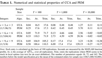
Numerical and statistical properties of CCA and PEM
 You have
Access
- 24
- Cited by