


1 INTRODUCTION
The nonlinear autoregressive distributed lag (NARDL) model is widely used to estimate the asymmetric cointegrating relationship between nonstationary variables. Since Shin, Yu, and Greenwood-Nimmo (Reference Shin, Yu, Greenwood-Nimmo, Horrace and Sickles2014) introduced the NARDL model, researchers have revisited many long-run relationships and modified linear ones using different slope coefficients based on the signs of the variables. For example, Borenstein, Cameron, and Gilbert (Reference Borenstein, Cameron and Gilbert1997) identified the so-called rockets and feathers in gasoline prices, showing that upward cost shocks in crude oil prices pass through faster than downward shocks, thus affecting other economic variables asymmetrically. Chesnes (Reference Chesnes2016) empirically confirms this feature using the NARDL model.
Despite its popularity, estimating the NARDL model using ordinary least squares (OLS) lacks theoretical foundation. Cho, Greenwood-Nimmo, and Shin (Reference Cho, Greenwood-Nimmo and Shin2026) noted that OLS suffers from an asymptotically singular matrix problem, and since then, no theoretical justification has emerged for estimating the NARDL parameter using OLS. Currently, many empirical studies continue to estimate the unknown parameter using OLS, without an established theory.
In this study, we revisit OLS and provide its large-sample theory. Although OLS suffers from the problem of an asymptotically singular matrix, we find that it consistently estimates the unknown parameter. Furthermore, we establish a theoretical basis for applying the Wald test principle to OLS by deriving its asymptotic distribution, which allows us to test for the NARDL hypothesis. OLS asymptotically follows a mixed normal distribution under some mild regularity conditions, validating the use of OLS for empirical analysis.
This study addresses a gap in the literature concerning NARDL estimation, although it is not the first to address the asymptotically singular matrix problem associated with NARDL. Cho et al. (Reference Cho, Greenwood-Nimmo and Shin2026) explained and resolved this problem by using a two-step procedure for estimating the NARDL parameter, termed two-step NARDL (2SNARDL). They separately estimate the long- and short-run parameters, following the method used by Engle and Granger (Reference Engle and Granger1987), which avoids the asymptotically singular matrix problem. We provide theoretical grounds to compare these two estimators by deriving the limit distribution of OLS and showing that the parameter targeted by OLS is estimated at the same convergence rate as 2SNARDL. From this, if the sample size is sufficiently large, OLS can estimate the parameter more straightforwardly than 2SNARDL. Meanwhile, 2SNARDL is more useful than OLS if the sample size is small and the asymptotic bias ignored by OLS can be efficiently removed.
Singular matrices are common in econometric asymptotics, particularly in multivariate regressions, and do not necessarily indicate the absence of a limit theory; rather, they lead to significant changes in that theory. In time-series analysis involving deterministic trends and nonstationary cointegrated regressors, researchers typically resolve singularity issues by applying multiple rates of convergence in various directions (see Phillips, Reference Phillips1995, and his subsequent works for early demonstrations). Similarly, singular matrices emerge in the context of maximum-likelihood (ML) and nonlinear least squares (NLS) estimations, letting researchers to find the limit distribution using higher-order approximation of the nonlinear model. From this, the convergence rate of the estimator becomes slower than the standard case (e.g., Teräsvirta, Reference Teräsvirta1994; Cho and White, Reference Cho and White2007, Reference Cho and White2010; Cho and Phillips, Reference Cho and Phillips2018).
In the current study’s OLS analysis, applying a higher-order approximation to its limit distribution is necessary, but challenging. Unlike ML and NLS, the model is linear, which means the higher-order expansion should directly apply to OLS, rather than the model itself. This task is particularly challenging, because it involves applying the higher-order expansion to the inverse matrix within OLS. Because the dimension of the matrix is arbitrary, approximating it using a higher-order expansion is not straightforward.
We address this issue by indirectly obtaining the asymptotic distribution of OLS. For this, we represent OLS as a transformation of other primitive estimators that do not suffer from a singular matrix problem, and then we derive their weak limits to achieve the desired limit distribution. This process elaborates on the Frisch–Waugh–Lovell (FWL) projection method in Park and Phillips (Reference Park and Phillips1988, Reference Park and Phillips1989) so that OLS can be represented by the primitive estimators without omitting any of its elements, identifying a channel through which the unknown parameters and the primitive estimators affect the limit distribution. Using this, we isolate the singular matrix problem and show that the convergence rate of OLS depends on the unknown parameter values.
The indirectly obtained limit distribution is useful for inferring the NARDL parameter. We can develop a test methodology using this limit distribution. In addition, using the limit distributions of the primitive estimators, we can establish an additional Wald test to compensate for the slower convergence rate of OLS. The primitive estimators prove to be super-consistent for the long-run parameter, which is also the same convergence rate as the long-run 2SNARDL estimator.
The limit theory of OLS guides proper empirical data analysis. In this demonstration, we analyze the empirical data provided by Romer and Romer (Reference Romer and Romer2010) to examine the long- and short-run relationships between U.S. GDP and fiscal exogenous shocks. Romer and Romer (Reference Romer and Romer2010) measure legislated exogenous tax changes related to the U.S. GDP using narrative records, such as presidential speeches and Congressional reports. By applying the NARDL model, we determine the long- and short-run relationships between tax increases and decreases in relation to the U.S. GDP. This empirical project also serves to illustrate our methodology in a standard setting.
We conduct the empirical project not only for demonstration, but also to identify how the long- and short-run relationships between U.S. GDP and tax decreases differ from those with tax increases. According to Romer and Romer (Reference Romer and Romer2010), exogenous tax changes are classified into those aimed at deficit reduction and those intended for long-run growth. All tax changes for deficit reduction relate to tax increases, while most changes for long-run growth involve tax decreases. The NARDL model, which we use, separates shocks into negative and positive ones and estimates their possibly different effects on the dependent variable. By applying the NARDL model, we analyze the long- and short-run relationships between the tax changes for deficit reduction and those for long-run growth in terms of U.S. GDP. Our investigation shows that the long- and short-run parameters are indeed symmetric, meaning that the tax changes for deficit reduction and those for long-run growth affect the U.S. GDP symmetrically.
The remainder of this article is structured as follows. Section 2 provides an overview of the NARDL model and discusses the asymptotically singular matrix problem associated with OLS. Section 3 defines primitive estimators and presents OLS as a bilinear transform of the primitive estimators. Section 4 discusses the limit distribution of OLS. Section 5 examines the large-sample properties of the standard Wald test for the NARDL hypothesis, and Section 6 presents Monte Carlo simulations for the Wald tests. Section 7 presents the empirical illustration. Finally, Section 8 concludes the article. All mathematical proofs are available in the Supplementary Material, in which we also provide other simulation evidence for OLS and empirical supplements.
Before moving to the next section, we present the notation used throughout this article. We provide the weak limit of an estimator by a stochastic integral. Denoting the weak limit by
$\int \mathcal {B}$
 or
$\int d\mathcal {B}$
 means
$\int _{0}^{1} \mathcal {B}(u) du$
 or
$\int _{0}^{1} d\mathcal {B}(u)$
 , respectively, where
$\mathcal {B}(\cdot )$
 is a Brownian motion.
2 MOTIVATION AND THE NARDL MODEL IN THE LITERATURE
This section briefly summarizes NARDL and motivates the current study.
2.1 NARDL and Error-Correction Models
We consider a NARDL(
$\!\! p,q$
 ) process augmented by a time trend:

where
$\boldsymbol {x}_{t}\in \mathbb {R}^{k}\, (k\in \mathbb {N})$
 ,
$\boldsymbol {x}_{t}^{+}:=\sum _{j=1}^{t}\Delta \boldsymbol {x}_{j}^{+}$
 ,
$\boldsymbol {x}_{t}^{-}:=\sum _{j=1}^{t}\Delta \boldsymbol {x}_{j}^{-}$
 ,
$\Delta \boldsymbol {x}_{t}^{+}:=\max [\mathbf {0},\Delta \boldsymbol {x}_{t}]$
 ,
$\Delta \boldsymbol {x}_{t}^{-}:=\min [\mathbf {0},\Delta \boldsymbol {x}_{t}]$
 ,
$\{e_{t},\mathcal {F}_{t}\}$
 is a martingale difference array (MDA), and
$\mathcal {F}_{t}$
 is the smallest
$\sigma $
 -algebra driven by
$\{y_{t-1},\boldsymbol {x}_{t}^{+},\boldsymbol {x}_{t}^{-},\, y_{t-2}, \boldsymbol {x}_{t-1}^{+},\boldsymbol {x}_{t-1}^{-},\ldots \}$
 such that
$\Delta \boldsymbol {x}_{t}$
 is a stationary process, and
$\Delta $
 denotes the differencing operator, so that
$\Delta \boldsymbol {x}_{t} := \boldsymbol {x}_{t} - \boldsymbol {x}_{t-1}$
 . Here, the
$\max $
 and
$\min $
 operators applied to a vector operate element-wise. The NARDL process in (1) is defined by introducing the asymmetric effect to the autoregressive distributed lag (ARDL) process proposed by Pesaran and Shin (Reference Pesaran, Shin and Strom1998). By supposing that the response of dependent variable
$y_{t}$
 to the positive and negative parts of
$\boldsymbol {x}_{t}$
 is possibly different, the NARDL process generalizes the ARDL process. If
$\boldsymbol {\theta }_{j*}^{+} = \boldsymbol {\theta }_{j*}^{-}$
 for each
$j$
 , the NARDL process reduces to the ARDL process. In addition, the NARDL process in (1) is more general than those defined by Shin et al. (Reference Shin, Yu, Greenwood-Nimmo, Horrace and Sickles2014) and Cho, Greenwood-Nimmo, and Shin (Reference Cho, Greenwood-Nimmo and Shin2023b), because the latter do not allow for a time trend on the right side.
The NARDL process is closely related to an error-correction representation. We first rewrite (1) as follows:

where
$\rho _{\ast }$
 ,
$\boldsymbol {\theta }_{\ast }^{+}$
 ,
$\boldsymbol {\theta }_{\ast }^{-}$
 ,
$\varphi _{j\ast }$
 (
$\!\! j=1,2,\ldots ,p-1$
 ),
$\boldsymbol {\pi }_{j\ast }^{+}$
 , and
$\boldsymbol {\pi }_{j\ast }^{-}$
 (
$\!\! j=0,1,\ldots ,q-1$
 ) are defined by the parameters in (1), as given in Cho et al. (Reference Cho, Greenwood-Nimmo and Shin2023b). Specifically,
$\rho _{*} := \sum _{j=1}^{p} \phi _{j*} - 1$
 ,
$\boldsymbol {\theta }_{*}^{+} := \sum _{j=0}^{q} \boldsymbol {\theta }_{j*}^{+}$
 ,
$\boldsymbol {\theta }_{*}^{-} := \sum _{j=0}^{q} \boldsymbol {\theta }_{j*}^{-}$
 ,
$\boldsymbol {\pi }_{0*}^{+} := \boldsymbol {\theta }_{0*}^{+},\;\;\;\;\boldsymbol {\pi }_{0*}^{-} := \boldsymbol {\theta }_{0*}^{-}$
 , and for
$\ell =1, 2, \ldots , p-1$
 and
$j = 1, 2, \ldots q-1$
 ,
$\varphi _{\ell *} := - \sum _{i=\ell +1}^{p} \phi _{i*}$
 ,
$\boldsymbol {\pi }_{j*}^{+} := -\sum _{i=j+1}^{q}\boldsymbol {\theta }_{i*}^{+}$
 ,
$\boldsymbol {\pi }_{j*}^{-} := -\sum _{i=j+1}^{q}\boldsymbol {\theta }_{i*}^{-}$
 , and
$\alpha _{*} = \alpha _{0*} + \xi _{*}$
 . By plugging these parameters into (2), the NARDL(
$\!\! p$
 ,
$q$
 ) process in (1) is obtained. For notational simplicity, we further rewrite this as

by letting
$\boldsymbol {\theta }_{\ast } := [\boldsymbol {\theta }_{*}^{+\prime }, \boldsymbol {\theta }_{*}^{-\prime }]^{\prime }$
 ,
$\ddot {\boldsymbol {x}}_{t-1} := [\boldsymbol {x}_{t-1}^{+\prime },\boldsymbol {x}_{t-1}^{-\prime }]^{\prime }$
 ,
$\boldsymbol {\kappa }_{*} :=[\boldsymbol {\varphi }_{*}^{\prime }, \boldsymbol {\pi }_{*}^{\prime }]^{\prime }$
 , and
$\boldsymbol {z}_{2t}:= [ \Delta \boldsymbol {y}_{t-1}^{\prime }, \Delta \widetilde {\boldsymbol {x}}_{t}^{\prime }]^{\prime }$
 , such that

Here, if
$y_{t-1}$
 is cointegrated with
$\ddot {\boldsymbol {x}}_{t-1}$
 , (2) can be rewritten into the following error-correction form:

such that the cointegration error is defined as
$u_{t-1} := y_{t-1} - \boldsymbol {\beta }_{\ast }^{\prime } \ddot {\boldsymbol {x}}_{t-1} - \zeta _{\ast } (t-1) - \nu _{\ast }$
 with
$ \boldsymbol {\beta }_{*}:= [\boldsymbol {\beta }_{*}^{+\prime }, \boldsymbol {\beta }_{*}^{-\prime }]^{\prime }$
 ,
$\boldsymbol {\beta }_{\ast }^{+}:=-(\boldsymbol {\theta }_{\ast }^{+}/\rho _{\ast })$
 ,
$\boldsymbol {\beta }_{\ast }^{-}:=-(\boldsymbol {\theta }_{\ast }^{-}/\rho _{\ast })$
 , and
$\zeta _{\ast } := -(\xi _{\ast }/\rho _{\ast })$
 . Here, the intercept
$\nu _{\ast }$
 is introduced so that
$\mathbb {E}[u_{t}] = 0$
 , and
$u_{t}$
 is assumed to be stationary and possibly correlated with
$\Delta \boldsymbol {y}_{t-1}$
 and
$\Delta \widetilde {\boldsymbol {x}}_{t}$
 . From this, it follows that
$\gamma _{\ast } = \alpha _{\ast } + \rho _{\ast } \nu _{\ast }$
 .
The NARDL process captures an asymmetric cointegrating relationship between nonstationary processes. If we let
$\boldsymbol {\mu }_{*}:=[\boldsymbol {\mu }_{\ast }^{+\prime }, \boldsymbol {\mu }_{\ast }^{-\prime }]^{\prime }$
 ,
$\boldsymbol {\mu }_{\ast }^{+} := \mathbb {E}[\Delta \boldsymbol {x}_{t}^{+}],$
 and
$\boldsymbol {\mu }_{\ast }^{-} := \mathbb {E}[\Delta \boldsymbol {x}_{t}^{-}]$
 , then
$\boldsymbol {\mu }_{\ast }^{+} + \boldsymbol {\mu }_{\ast }^{-} \equiv \mathbb {E}[\Delta \boldsymbol {x}_{t}]$
 by construction. Therefore, if we further let
$\boldsymbol {s}_{t}^{+} := \Delta \boldsymbol {x}_{t}^{+} - \boldsymbol {\mu }_{\ast }^{+}$
 and
$\boldsymbol {s}_{t}^{-} := \Delta \boldsymbol {x}_{t}^{-} - \boldsymbol {\mu }_{\ast }^{-}$
 , it follows that

From (4),
$\ddot {\boldsymbol {x}}_{t}$
 is clearly a unit-root process with nonzero time trends. Moreover,
$\Delta y_{t}$
 is not necessarily distributed around zero, even when
$\boldsymbol {x}_{t}$
 is a unit-root process without a time trend. From (3), we have

so that if
$d_{t} := \Delta y_{t} - \delta _{\ast }$
 , then

This fact implies that
$y_{t}$
 is a unit-root process with a deterministic time trend, which has further implications. First, even when
$\mathbb {E}[\boldsymbol {x}_{t}] = \mathbf {0}$
 , the NARDL model captures a cointegrating relationship between the variables without and with time trend, viz.,
$\boldsymbol {x}_{t}$
 and
$y_{t}$
 . Second, the NARDL model includes the time trend in (2) as an explanatory variable by noting that the trend in
$y_{t}$
 could also be influenced by exogenous factors other than the NARDL effect. If the estimated coefficient of the time trend is insignificant, it signals that the trend in
$y_{t}$
 is sorely sourced from the NARDL effect.
2.2 OLS for NARDL and Asymptotic Singular Matrix
Shin et al. (Reference Shin, Yu, Greenwood-Nimmo, Horrace and Sickles2014) estimate (2) by OLS without distinguishing the long- and short-run equations, which is now very popular in the empirical literature. For this examination, we first let

so that
$\boldsymbol {r}_{t-1} = [\ddot {\boldsymbol {x}}_{t-1}^{\prime }, (t-1), 1]^{\prime }$
 . Here,
$\boldsymbol {z}_{t} \in \mathbb {R}^{2 + p + 2k(1+q)}$
 is partitioned into two variables such that
$\boldsymbol {z}_{1t} \in \mathbb {R}^{3+2k}$
 and
$\boldsymbol {z}_{2t} \in \mathbb {R}^{p+2kq-1}$
 . Next, we let
$\boldsymbol {\alpha }_{\ast } := [ \begin {array}{cccc:c} \rho _{\ast } & \boldsymbol {\theta }_{\ast }^{\prime } & \xi _{\ast } & \alpha _{\ast } & \boldsymbol {\kappa }_{\ast }' \end {array} ]^{\prime }$
 . From this, the OLS estimator is written as

For later purposes, we partition
$\widehat {\boldsymbol {\theta }}_{T}$
 and
$\widehat {\boldsymbol {\kappa }}_{T}$
 into
$[\widehat {\boldsymbol {\theta }}_{T}^{+\prime }, \widehat {\boldsymbol {\theta }}_{T}^{-\prime }]^{\prime }$
 and
$[\widehat {\boldsymbol {\varphi }}_{T}^{\prime }, \widehat {\boldsymbol {\pi }}_{T}^{\prime }]^{\prime } \equiv [\widehat {\boldsymbol {\varphi }}_{T}^{\prime }, \widehat {\boldsymbol {\pi }}_{T}^{+\prime }, \widehat {\boldsymbol {\pi }}_{T}^{-\prime }]^{\prime }$
 , respectively.
Despite its popularity, there is no theoretical foundation for the OLS. This is mainly attributed to the asymptotically singular matrix problem. Even under mild regularity conditions, the OLS estimator suffers from an asymptotically singular matrix problem. For this discussion, we impose the following conditions, which are standard in the literature.
Assumption 1.
-
(i) $\{ (\Delta y_{t}, \Delta \boldsymbol {x}_{t}^{\prime }, u_{t})^{\prime } \in \mathbb {R}^{k+2}: t= \ldots , -1, 0, 1, \ldots \}$
 is a strictly stationary
$\phi $
-mixing process of size
$-r/(2(r-1))$
or
$\alpha $
-mixing process of size
$-r/(r-2)$
and
$r> 2$
.
-
(ii) $\mathbb {E}[\vert \Delta x_{ti} \vert ^{r}] < \infty \, (i = 1, 2, \ldots , k)$
,
$\mathbb {E}[\vert u_{t} \vert ^{r}] < \infty $
,
$\mathbb {E}[\vert e_{t}\vert ^{2}] < \infty $
, and
$\delta _{\ast } \neq 0$
, where
$x_{ti}$
is the
$i$
-th row element of
$\boldsymbol {x}_{t}$
. -
(iii) $\boldsymbol {\Sigma }_{\ast } := \lim _{T\to \infty } \text {var}[T^{-1/2} \sum _{t=1}^{T} \boldsymbol {w}_{t} ]$
is positive definite, where $$ \begin{align*} \boldsymbol{w}_{t} := [\begin{array}{c:c} \boldsymbol{w}_{1t}^{\prime} & \boldsymbol{w}_{2t}^{\prime} \end{array}] := [ \begin{array}{cc:ccc} \boldsymbol{s}_{t-1}^{\prime } & u_{t-1} & e_{t} & e_{t} u_{t-1} & e_{t}\boldsymbol{z}_{2t}' \end{array} ]^{\prime } \end{align*} $$
and $\boldsymbol {s}_{t-1} := [\boldsymbol {s}_{t-1}^{+\prime }, \boldsymbol {s}_{t-1}^{- \prime }]^{\prime }$
. -
(iv) For some $\boldsymbol {\alpha }_{\ast }$
with
$\rho _{\ast }< 0$
,
$\Delta y_{t}$
is generated by (2) such that
$\vert L_{\ast } \vert> 1$
, where
$1 - \sum _{j=1}^{p} \phi _{j\ast }L_{\ast }^{j} \equiv 0$
. -
(v) $\{e_{t}, \mathcal {F}_{t}\}$
is an MDA such that
$\mathbb {E}[e_{t}^{2} \vert \mathcal {F}_{t}] = \sigma _{e}^{2}$
.


Remarks.
-
(a) Under the same assumption, we investigate the limit behavior of the OLS estimator below.
-
(b) Assumptions 1(i and ii) assume mixing and moment conditions to apply the functional central limit theorem (FCLT) to a partial-sum data process. The FCLT is popular for deriving the limit distribution of the OLS applied to estimate a cointegrating relationship (e.g., Phillips and Hansen, Reference Phillips and Hansen1990; Phillips, Reference Phillips1991; White, Reference White2001, Chap. 7).
-
(c) Assumption 1(iv) assumes $\rho _{\ast }< 0$
for a cointegrating relationship between
$y_{t}$
and
$\ddot {\boldsymbol {x}}_{t}$
. If no cointegrating relationship exists, so that if
$\boldsymbol {\beta }_{*} = \mathbf {0}$
and
$\zeta _{\ast } = 0$
, then it follows from (3) that $$ \begin{align*} y_{t} = \alpha_{\ast}+ \sum_{j=1}^{p} \phi_{j\ast}y_{t-j} + \boldsymbol{\pi}_{\ast}^{\prime } \Delta \widetilde{\boldsymbol{x}}_{t} + e_{t}. \end{align*} $$
Assumption 1(iv), however, implies that $y_{t}$
is a stationary process, contradicting the assumption that
$y_{t}$
is a unit-root process. From this, it is necessary to assume
$\rho _{\ast } = 0$
for
$(\boldsymbol {\beta }_{\ast }^{\prime }, \zeta _{\ast })^{\prime } = \mathbf {0}$
. In this study, we assume the cointegrating relationship established by (3). -
(d) Although it is not our main interest, Pesaran, Shin, and Smith (Reference Pesaran, Shin and Smith2001) and Banerjee, Dolado, and Mestre (Reference Banerjee, Dolado and Mestre1998) have previously examined estimating the unknown parameter by OLS under $\rho _{\ast } = 0$
. They assumed a linear model and developed a testing methodology for
$\rho _{*} = 0$
. Their methodology is applicable even in the context of NARDL, because assuming no cointegration under the condition of linearity is equivalent to assuming
$\boldsymbol {\beta }_{*} = \mathbf {0}$
and
$\zeta _{*} = 0$
. -
(e) Assumption 1(v) is a standard condition for the error term in the ARDL and NARDL processes (e.g., Pesaran and Shin, Reference Pesaran, Shin and Strom1998; Pesaran et al., Reference Pesaran, Shin and Smith2001; Shin et al., Reference Shin, Yu, Greenwood-Nimmo, Horrace and Sickles2014; Cho et al., Reference Cho, Greenwood-Nimmo and Shin2026).


We now show how the asymptotically singular matrix problem is associated with the OLS. For this, we provide the following lemma.
Lemma 1. Under Assumption 1,
-
(i)
$$ \begin{align*} \mathbf{D}_{1}^{-1} \left(\sum_{t=1}^{T} \boldsymbol{z}_{1t}\boldsymbol{z}_{1t}^{\prime} \right) \mathbf{D}_{1}^{-1} \stackrel{\mathbb{P}}{\to} \mathbf{M}_{11} := \left[\begin{array}{c:c} \left[ \begin{array}{@{}c@{}} \frac13 \delta_{*} \\ \frac13 \boldsymbol{\mu}_{*} \\ \frac13 \\ \frac12 \end{array} \right] [\delta_{*}, \boldsymbol{\mu}_{*}^{\prime}, 1] & \left[ \begin{array}{@{}c@{}} \frac12 \delta_{*} \\ \frac12 \boldsymbol{\mu}_{*} \\ \frac12 \\ 1 \end{array} \right] \end{array} \right], \end{align*} $$
where $\mathbf {D}_{1} := \textrm {diag}[T^{3/2} \mathbf {I}_{2+2k}, T^{1/2}]$
; -
(ii) $\mathbf {D}_{2}^{-1} \left (\sum _{t=1}^{T} \boldsymbol {z}_{2t}\boldsymbol {z}_{2t}^{\prime } \right ) \mathbf {D}_{2}^{-1} \stackrel {\mathbb {P}}{\to } \mathbf {M}_{22} := \mathbb {E}[\boldsymbol {z}_{2t} \boldsymbol {z}_{2t}^{\prime }]$
, where
$\mathbf {D}_{2} := T^{1/2}\mathbf {I}_{p+2kq-1}$
; -
(iii)
$$ \begin{align*} \mathbf{D}_{2}^{-1} \left( \sum_{t=1}^{T} \boldsymbol{z}_{2t} \boldsymbol{z}_{1t}^{\prime} \right) \mathbf{D}_{1}^{-1} \stackrel{\mathbb{P}}{\to} \mathbf{M}_{21} := \left[\!\!\!\! \begin{array}{c:c} \left[ \begin{array}{@{}c@{}} \frac{1}{2}\delta_{\ast} \boldsymbol{\iota}_{p-1} \\ \frac{1}{2} \boldsymbol{\iota}_{q}\otimes \boldsymbol{\mu}_{\ast} \end{array} \right] [ \delta_{*}, \boldsymbol{\mu}_{*}^{\prime}, 1 ] & 2 \left[ \begin{array}{@{}c@{}} \frac{1}{2}\delta_{\ast} \boldsymbol{\iota}_{p-1} \\ \frac{1}{2} \boldsymbol{\iota}_{q}\otimes \boldsymbol{\mu}_{\ast} \end{array} \right] \end{array}\!\!\!\!\right], \end{align*} $$
where for each $\ell \in \mathbb {N}$
,
$\boldsymbol {\iota }_{\ell } := [ 1, 1, \ldots , 1]^{\prime } \in \mathbb {R}^{\ell }$
; -
(iv)
$$ \begin{align*} \mathbf{D}^{-1} \left( \sum_{t=1}^{T} \boldsymbol{z}_{t} \boldsymbol{z}_{t}^{\prime }\right) \mathbf{D}^{-1} \stackrel{\mathbb{P}}{\to} \mathbf{M} := \left[ \begin{array}{@{}cc@{}} \mathbf{M}_{11} & \mathbf{M}_{12} \\ \mathbf{M}_{21} & \mathbf{M}_{22} \end{array} \right], \end{align*} $$which is singular, where $\mathbf {D} := \textrm {diag}[ \mathbf {D}_{1}, \mathbf {D}_{2}]$
and
$\mathbf {M}_{12} := \mathbf {M}_{21}^{\prime }$
.


Here,
$\mathbf {M}$
 is singular because its first
$(1+2k)$
 columns are proportional to the
$(2+2k)$
 -th column.
Remarks.
-
(a) Lemma 1 clearly implies that the theoretical foundation of the OLS cannot be established without tackling the asymptotically singular matrix problem. The asymptotically singular matrix problem arises from the deterministic time trend in the regressors. Specifically, $\mathbb {E}[\Delta y_{t-1}] \neq 0$
by (5), so that
$y_{t-1}$
is an integrated series with a deterministic time trend. Likewise, both
$\boldsymbol {x}_{t-1}^{+}$
and
$\boldsymbol {x}_{t-1}^{-}$
are integrated series with deterministic time trends. Therefore, all of
$y_{t-1}$
,
$\ddot {\boldsymbol {x}}_{t-1}$
, and
$(t-1)$
are driven by the time trend, leading to the asymptotically singular matrix problem. This aspect is also evident from Lemma 1. The first
$(2+2k)$
columns of
$\mathbf {M}$
are proportional to each other, and they are the terms involved with
$y_{t-1}$
,
$\ddot {\boldsymbol {x}}_{t-1}$
, and
$(t-1)$
. -
(b) Cho et al. (Reference Cho, Greenwood-Nimmo and Shin2026) note the asymptotically singular matrix and estimate the unknown long-run parameters by first removing the trends from $y_{t-1}$
and
$\ddot {\boldsymbol {x}}_{t-1}$
, proposing 2SNARDL estimation. We prove Lemma 1 in the Supplementary Material by extending Lemma 1 of Cho et al. (Reference Cho, Greenwood-Nimmo and Shin2026). Their lemma demonstrates another singular matrix problem by supposing no time trend in (1). Lemma 1 verifies that augmenting the time trend on the right side is not helpful in eliminating the singular matrix problem.Figure 1Asymptotic singularity of the matrix ${\mathbf{D}}^{-1} ({\sum}_{t=1}^{T} {\boldsymbol{z}}_{t} {\boldsymbol{z}}_{t}^{\prime}) {\mathbf{D}}^{-1} $
. Figure 1(a) shows the scatter diagram between the sample size and the averaged minimum diagonal element of
${\mathbf{D}}^{-1} ({\sum}_{t=1}^{T} {\boldsymbol{z}}_{t} {\boldsymbol{z}}_{t}^{\prime}) {\mathbf{D}}^{-1} $
obtained by imposing the DGP condition used to examine the power properties of the Wald tests in Section 6. Figure 1(b) shows the scatter diagram between the sample size and the averaged determinant
$\times 10^{12}$
of the same matrix. For the scatter diagrams, 10,000 independent experiments are repeated to compute the averages from the 10,000 independent matrices.Figure 1 Long description
The image consists of two vertically stacked line graphs with grid backgrounds.
Top Panel (a) Average of Traces
* The x-axis is labeled sample size and ranges from 0 to 500 in increments of 25.
* The y-axis is labeled Minimum Diagonal Element and ranges from 0.0025 to 0.0065.
* The data points show a steep asymptotic decrease from approximately 0.0063 at a sample size of 25 down to 0.0029 at a sample size of 200. From 200 to 500, the curve flattens significantly, fluctuating slightly between 0.0025 and 0.0029.
Bottom Panel (b) Average of Determinants times 10 super 12
* The x-axis is labeled sample size and ranges from 0 to 500 in increments of 25.
* The y-axis is labeled Determinant and ranges from 0 to 2.2.
* The data shows a very sharp exponential decay. At a sample size of 25, the determinant is approximately 2.1. It drops precipitously to 0.3 at a sample size of 50 and reaches near-zero values by a sample size of 125. The line remains flat and close to the x-axis for all sample sizes from 125 to 500.
-
(c) We can easily verify the asymptotically singular matrix problem by conducting simple Monte Carlo simulations. By exploiting the model and data-generating process (DGP) conditions used to examine the power properties of the Wald tests in Section 6, we compute the minimum diagonal element and determinant of $\mathbf {D}^{-1} (\sum _{t=1}^{T} \boldsymbol {z}_{t}\boldsymbol {z}_{t}^{\prime }) \mathbf {D}^{-1}$
for
$T=$
25, 50, 75, 100, 125,
$\ldots $
, 475, and 500. After iterating 10,000 independent experiments, Figure 1(a) draws a scatter diagram between
$T$
and the average of the 10,000 minimum diagonal elements. From this, we can see that the minimum diagonal element converges to a finite number, indicating that
$\mathbf {D}^{-1} (\sum _{t=1}^{T} \boldsymbol {z}_{t}\boldsymbol {z}_{t}^{\prime }) \mathbf {D}^{-1} = O_{\mathbb {P}}(1)$
. Meanwhile, Figure 1(b) draws a scatter diagram between
$T$
and the average of the 10,000 determinants
$\times 10^{12}$
. This second figure shows that the determinant converges to zero, meaning that
$\mathbf {D}^{-1} (\sum _{t=1}^{T} \boldsymbol {z}_{t}\boldsymbol {z}_{t}^{\prime }) \mathbf {D}^{-1}$
is asymptotically singular. This corroborates Lemma 1. -
(d) Singular matrices often appear in econometric asymptotics, especially in multivariate regressions. These matrices do not necessarily indicate the absence of a limit theory; rather, they typically lead to significant changes in that theory. In time-series analysis, when dealing with deterministic trends and nonstationary cointegrated regressors, researchers use multiple rates of convergence in different directions to address this issue (e.g., Phillips, Reference Phillips1995, and his subsequent works). In the cases of ML and NLS estimations, researchers obtain the limit distribution by applying higher-order approximations to nonlinear models, resulting in a slower convergence rate compared to the standard case (e.g., Teräsvirta, Reference Teräsvirta1994; Cho and White, Reference Cho and White2007, Reference Cho and White2010; Cho and Phillips, Reference Cho and Phillips2018).
-
(e) In the current context, it is not straightforward to apply a higher-order expansion to OLS. The model is already linear, unlike ML and NLS. This means that it is necessary to apply the higher-order expansion to OLS itself. However, given that the dimension of $(\sum _{t=1}^{T} \boldsymbol {z}_{t}\boldsymbol {z}_{t}^{\prime })^{-1}$
is determined by
$k$
,
$p$
, and
$q$
, and they can be given arbitrarily, the task becomes challenging.


3 AN ALTERNATIVE REPRESENTATION OF THE OLS ESTIMATOR
Owing to the complexity of the higher-order expansion, we use a different approach to obtain the desired limit distribution. We represent the OLS estimator as a transformation of other primitive estimators that do not suffer from an asymptotic singularity problem.
3.1 Alternative Representation
We achieve the alternative representation in two steps. First, we estimate the long- and short-run parameters using OLS and represent the OLS estimator
$\widehat {\boldsymbol {\alpha }}_{T}$
 as a bilinear transformation of the long- and short-run OLS estimators. Next, we express the long- and short-run OLS estimators as other bilinear transformations of further primitive estimators that do not suffer from an asymptotically singular matrix problem.
3.1.1 First Step: Representing OLS Estimator by Long- and Short-Run Estimators
We estimate the long-run parameter using OLS. That is, after specifying the long-run equation

by letting
$\boldsymbol {\upsilon }_{\ast } := [\boldsymbol {\beta }_{\ast }^{\prime }, \zeta _{\ast }, \nu _{\ast } ]'$
 , we let the long-run OLS estimator be

For later purposes, we let
$\widetilde {u}_{t-1} := y_{t-1} - \boldsymbol {r}_{t-1}^{\prime } \widetilde {\boldsymbol {\upsilon }}_{T}$
 and partition
$\widetilde {\boldsymbol {\beta }}_{T}$
 such that
$\widetilde {\boldsymbol {\beta }}_{T} \equiv [\widetilde {\boldsymbol {\beta }}_{T}^{+\prime }, \widetilde {\boldsymbol {\beta }}_{T}^{-\prime }]^{\prime }$
 .
We next estimate the short-run parameter by letting
$\boldsymbol {\omega }_{*} := [\rho _{*}, \boldsymbol {\eta }_{*}^{\prime }, \psi _{*}, \gamma _{*}, \boldsymbol {\kappa }_{*}^{\prime } ]^{\prime }$
 , such that
$\boldsymbol {\eta }_{\ast } := \boldsymbol {\theta }_{\ast } + \rho _{\ast }\boldsymbol {\beta }_{\ast }$
 and
$\psi _{\ast } := \xi _{\ast } + \rho _{\ast } \zeta _{\ast }$
 , and
$\dot {\boldsymbol {z}}_{t} := [ u_{t-1}, \boldsymbol {r}_{t-1}^{\prime }, \boldsymbol {z}_{2t}^{\prime } ]^{\prime }$
 to specify the error-correction model

We obtain this equation by combining (2) and (6) and estimate the parameters in (7) by

estimating the short-run parameter
$\boldsymbol {\omega }_{*}$
 . Note that
$\widetilde {\boldsymbol {\omega }}_{T}$
 is obtained by replacing
$u_{t-1}$
 with
$\widetilde {u}_{t-1}$
 . For later purposes, we partition
$\boldsymbol {\eta }_{*}$
 into
$[\boldsymbol {\eta }_{*}^{+\prime }, \boldsymbol {\eta }_{*}^{-\prime }]^{\prime }$
 .
The long- and short-run OLS estimators have a regular relationship in terms of the OLS estimator
$\widehat {\boldsymbol {\alpha }}_{T}$
 . The following proposition reveals the relationship.
Proposition 1. Under Assumption 1,
$\widehat {\boldsymbol {\alpha }}_{T} = \mathbf {R}_{T} \widetilde {\boldsymbol {\omega }}_{T}$
 , where

Remarks.
-
(a) By Proposition 1, the OLS estimator $\widehat {\boldsymbol {\alpha }}_{T}$
is now represented as a bilinear transformation between the long- and short-run OLS estimators
$\widetilde {\boldsymbol {\upsilon }}_{T}$
and
$\widetilde {\boldsymbol {\omega }}_{T}$
. That is, $$ \begin{align*} \widehat{\boldsymbol{\alpha}}_{T} = [\widetilde{\rho}_{T}, \, -\widetilde{\rho}_{T} \widetilde{\boldsymbol{\beta}}_{T}^{\prime} + \widetilde{\boldsymbol{\eta}}_{T}^{\prime}, \, -\widetilde{\rho}_{T} \widetilde{\zeta}_{T} + \widetilde{\psi}_{T}, \, -\widetilde{\rho}_{T} \widetilde{\nu}_{T} + \widetilde{\gamma}_{T}, \, \widetilde{\boldsymbol{\kappa}}_{T}^{\prime} ]^{\prime}. \end{align*} $$
If both $\widetilde {\boldsymbol {\upsilon }}_{T}$
and
$\widetilde {\boldsymbol {\omega }}_{T}$
are consistent for
$\boldsymbol {\upsilon }_{*}$
and
$\boldsymbol {\omega }_{*}$
, respectively, it follows that $$ \begin{align*} \widehat{\boldsymbol{\alpha}}_{T} \stackrel{\mathbb{P}}{\to} [\rho_{*}, \, -\rho_{*} \boldsymbol{\beta}_{*} + \boldsymbol{\eta}_{*}^{\prime}, \, -\rho_{*} \zeta_{*} + \psi_{*}, \, -\rho_{*} \nu_{*} + \gamma_{*}, \, \boldsymbol{\kappa}_{*}^{\prime} ]^{\prime} = [\rho_{*}, \, \boldsymbol{\theta}_{*}, \, \xi_{*}, \, \alpha_{*}, \, \boldsymbol{\kappa}_{*}^{\prime} ]^{\prime} \end{align*} $$
by noting that $\boldsymbol {\eta }_{*} = \mathbf {0}$
and
$\psi _{*} = 0$
. -
(b) Proposition 1 follows by applying Lemma A.2 in the Supplementary Material. By letting $y_{t}$
,
$\boldsymbol {x}_{t}$
,
$\boldsymbol {z}_{t}$
, and
$\boldsymbol {w}_{t}$
of Lemma A.2 in the Supplementary Material be
$\Delta y_{t}$
,
$y_{t-1}$
,
$\boldsymbol {r}_{t-1}$
, and
$\boldsymbol {z}_{2t}$
of (7), respectively, Proposition 1 follows. Here,
$\widehat {\boldsymbol {v}}_{t}$
in Lemma A.2 in the Supplementary Material corresponds to
$\widetilde {u}_{t-1}$
. Lemma A.2 in the Supplementary Material is established by elaborating on the FWL projection method in Park and Phillips (Reference Park and Phillips1988, Reference Park and Phillips1989). It complements the FWL method by augmenting a representation for the estimator ignored by FWL, so that the OLS estimator
$\widehat {\boldsymbol {\alpha }}_{T}$
could be written without omitting any of its element as given in Proposition 1. By this feature, we call Lemma A.2 in the Supplementary Material the augmented FWL (AFWL). For the goal to derive the joint limit distribution of
$\widehat {\boldsymbol {\alpha }}_{T}$
, it is important to derive the joint limit distributions of the long- and short-run OLS estimators without omitting any of its element, but FWL omits the representation of the coefficient, if its variable is concentrated out. For this reason, we complement FWL using AFWL and provide the alternative representation for
$\widehat {\boldsymbol {\alpha }}_{T}$
.


3.1.2 Second Step: Representing Long- and Short-Run Estimators by Primitive Estimators
Although Proposition 1 represents
$\widehat {\boldsymbol {\alpha }}_{T}$
 as a bilinear transformation between the long- and short-run OLS estimators, they both suffer from asymptotically singular matrix problems. It is mainly because
$\widetilde {\boldsymbol {\upsilon }}_{T}$
 and
$\widetilde {\boldsymbol {\omega }}_{T}$
 are defined by regressors including
$\ddot {\boldsymbol {x}}_{t-1}$
 and
$(t-1)$
 that are driven by the time trend (see Lemma A.3 in the Supplementary Material). Therefore, we again represent both estimators using other primitive estimators that do not suffer from an asymptotically singular matrix problem.
Long-Run Estimator: We first represent the long-run OLS estimator
$\widetilde {\boldsymbol {\upsilon }}_{T}$
 using other estimators. Note that both (4) and (6) imply that

This representation is obtained by collecting the deterministic time trend
$(t-1)$
 and the remainder
$\mathbf {m}_{t-1}$
 in (4) as regressors. However,
$\mathbf {m}_{t-1}$
 is unobservable. So, we first predict it by estimating the unknown parameters
$\boldsymbol {\mu }_{*}$
 in (4):

and regressing
$y_{t-1}$
 against
$\ddot {\boldsymbol {r}}_{t-1}:= [ \ddot {\mathbf {m}}_{t-1}^{\prime }, (t-1), 1 ]^{\prime }$
 , to obtain

For later purposes, we partition
$\ddot {\boldsymbol {\beta }}_{T}$
 such that
$\ddot {\boldsymbol {\beta }}_{T} \equiv [\ddot {\boldsymbol {\beta }}_{T}^{+\prime }, \ddot {\boldsymbol {\beta }}_{T}^{-\prime }]^{\prime }$
 and let
$\ddot {u}_{t-1} := y_{t-1} - \ddot {\boldsymbol {r}}_{t-1}^{\prime } \ddot {\boldsymbol {\upsilon }}_{T}$
 .
The interrelationship between the long-run OLS and primitive estimators is stated in the following proposition.
Proposition 2. Given Assumption 1,
$\widetilde {\boldsymbol {\upsilon }}_{T} := [ \widetilde {\boldsymbol {\beta }}_{T}^{\prime },\, \widetilde {\zeta }_{T},\, \widetilde {\nu }_{T} ]^{\prime } = \mathbf {P}_{T} \ddot {\boldsymbol {\upsilon }}_{T} = [ \ddot {\boldsymbol {\beta }}_{T}^{\prime }, \, \ddot {\vartheta }_{T} -\ddot {\boldsymbol {\mu }}_{T}^{\prime } \ddot {\boldsymbol {\beta }}_{T}, \, \ddot {\nu }_{T} ]^{\prime }$
 , where

Remarks.
-
(a) By Proposition 2, the long-run OLS estimator $\widetilde {\boldsymbol {\upsilon }}_{T}$
is represented as a bilinear transformation between the primitive estimators,
$\ddot {\boldsymbol {\mu }}_{T}$
and
$\ddot {\boldsymbol {\upsilon }}_{T}$
. This representation is particularly useful, because neither
$\ddot {\boldsymbol {\mu }}_{T}$
nor
$\ddot {\boldsymbol {\upsilon }}_{T}$
suffers from an asymptotically singular matrix problem (see Lemma 2 below). -
(b) If both $\ddot {\boldsymbol {\mu }}_{T}$
and
$\ddot {\boldsymbol {\upsilon }}_{T}$
are consistent for
$\boldsymbol {\mu }_{*}$
and
$\bar {\boldsymbol {\upsilon }}_{*}$
, respectively, $$ \begin{align*} \widetilde{\boldsymbol{\upsilon}}_{T} = [ \ddot{\boldsymbol{\beta}}_{T}^{\prime}, \, \ddot{\vartheta}_{T} -\ddot{\boldsymbol{\mu}}_{T}^{\prime} \ddot{\boldsymbol{\beta}}_{T}, \, \ddot{\nu}_{T} ]^{\prime} \stackrel{\mathbb{P}}{\to} [ \boldsymbol{\beta}_{*}^{\prime}, \, \vartheta_{*} - \boldsymbol{\mu}_{*}^{\prime} \boldsymbol{\beta}_{*}, \, \nu_{*} ]^{\prime} = [ \boldsymbol{\beta}_{*}^{\prime}, \, \zeta_{*}, \, \nu_{*} ]^{\prime} =: \boldsymbol{\upsilon}_{*} \end{align*} $$
by noting that $\vartheta _{\ast } := \boldsymbol {\beta }_{\ast }^{\prime } \boldsymbol {\mu }_{\ast } + \zeta _{\ast }$
, leading to the consistency of
$\widetilde {\boldsymbol {\upsilon }}_{T}$
for
$\boldsymbol {\upsilon }_{*}$
. Furthermore,
$\widetilde {u}_{t-1} = \ddot {u}_{t-1}$
using the definition of
$\ddot {\mathbf {m}}_{t-1} := \ddot {\boldsymbol {x}}_{t-1} - (t-1) \ddot {\boldsymbol {\mu }}_{T}$
. -
(c) Proposition 2 is also established by AFWL. If we let $y_{t-1}$
,
$\ddot {\boldsymbol {x}}_{t-1}^{\prime }$
,
$(t-1)$
, and
$1$
be
$y_{t}$
,
$\boldsymbol {x}_{t}$
,
$\boldsymbol {z}_{t}$
, and
$\boldsymbol {w}_{t}$
, respectively, in Lemma A.2 in the Supplementary Material, then Proposition 2 follows.


Short-Run Estimator: Next, we represent the short-run OLS estimator
$\widetilde {\boldsymbol {\omega }}_{T}$
 as a bilinear transformation between two other estimators that do not suffer from an asymptotically singular matrix problem. This representation is parallel to the one for the long-run OLS estimator. As both
$\ddot {\boldsymbol {x}}_{t-1}$
 and
$(t-1)$
 on the right side of (7) are driven by the deterministic trend, we reparameterize (7) using (4):

Here, the coefficient of
$(t-1)$
 is obtained as
$\varsigma _{*}$
 by collecting the coefficients of the time trends in
$\ddot {\boldsymbol {x}}_{t-1}$
 and
$(t-1)$
 , but the coefficient of
$\mathbf {m}_{t-1}$
 keeps the same as that of
$\ddot {\boldsymbol {x}}_{t-1}$
 on the right side of (7).
We estimate the unknown parameters in (9) by OLS. For this, we replace
$u_{t-1}$
 and
$\mathbf {m}_{t-1}$
 in (9) with
$\ddot {u}_{t-1}$
 and
$\ddot {\mathbf {m}}_{t-1}$
 , respectively, as they are unobservable. By letting
$\ddot {\boldsymbol {z}}_{t} := [ \begin {array}{c:c:cc} \ddot {u}_{t-1} & \ddot {\boldsymbol {r}}_{t-1}^{\prime } & \boldsymbol {z}_{2t}^{\prime } \end {array} ]^{\prime }$
 , the parameter estimator is obtained as follows:

estimating

Here, for later purposes, we let
$\ddot {\boldsymbol {\eta }}_{T} \equiv [\ddot {\boldsymbol {\eta }}_{T}^{+\prime }, \ddot {\boldsymbol {\eta }}_{T}^{-\prime } ]^{\prime }$
 and
$\ddot {\boldsymbol {\kappa }}_{T} \equiv [\ddot {\boldsymbol {\varphi }}_{T}^{\prime }, \ddot {\boldsymbol {\pi }}_{T}^{\prime }]^{\prime } \equiv [\ddot {\boldsymbol {\varphi }}_{T}^{\prime }, \ddot {\boldsymbol {\pi }}_{T}^{+\prime }, \ddot {\boldsymbol {\pi }}_{T}^{-\prime }]^{\prime }$
 . In addition, we separately estimate
$\psi _{\ast }$
 by
$\ddot {\psi }_{T} := -\ddot {\boldsymbol {\mu }}_{T}^{\prime } \ddot {\boldsymbol {\eta }}_{T} + \ddot {\varsigma }_{T}$
 by applying the plug-in principle to
$\varsigma _{*} := \boldsymbol {\mu }_{*}^{\prime } \boldsymbol {\eta }_{*} + \psi _{*}$
 .
The interrelationship between the short-run OLS and primitive estimators,
$\widetilde {\boldsymbol {\omega }}_{T}$
 and
$\ddot {\boldsymbol {\tau }}_{T}$
 , is stated in the following proposition.
Proposition 3. Given Assumption 1,
$\widetilde {\boldsymbol {\omega }}_{T} = \mathbf {Q}_{T} \ddot {\boldsymbol {\tau }}_{T}$
 , where

Remarks.
-
(a) By Proposition 3, the short-run OLS estimator $\widetilde {\boldsymbol {\omega }}_{T}$
is represented as a bilinear transformation between
$\ddot {\boldsymbol {\mu }}_{T}$
and
$\ddot {\boldsymbol {\tau }}_{T}$
, which do not suffer from asymptotically singular matrix problems (see Lemma 2 below). -
(b) If both $\ddot {\boldsymbol {\mu }}_{T}$
and
$\ddot {\boldsymbol {\tau }}_{T}$
are consistent for
$\boldsymbol {\mu }_{*}$
and
$\boldsymbol {\tau }_{*}$
, respectively, it follows that $$ \begin{align*} \widetilde{\boldsymbol{\omega}}_{T} &= [\ddot{\rho}_{T}, \, \ddot{\boldsymbol{\eta}}_{T}^{\prime}, \, -\ddot{\boldsymbol{\mu}}_{T}^{\prime} \ddot{\boldsymbol{\eta}}_{T} + \ddot{\varsigma}_{T}, \, \ddot{\gamma}_{T}, \, \ddot{\boldsymbol{\kappa}}_{T}^{\prime} ]^{\prime} \\ &\stackrel{\mathbb{P}}{\to} [\rho_{*}, \, \boldsymbol{\eta}_{*}^{\prime}, \, -\boldsymbol{\mu}_{*}^{\prime} \boldsymbol{\eta}_{*} + \varsigma_{*}, \, \gamma_{*}, \, \boldsymbol{\kappa}_{*}^{\prime} ]^{\prime} = [\rho_{*}, \, \boldsymbol{\eta}_{*}^{\prime}, \, \psi_{*}, \, \gamma_{*}, \, \boldsymbol{\kappa}_{*}^{\prime} ]^{\prime} =: \boldsymbol{\omega}_{*} \end{align*} $$
by noting that $\varsigma _{*} := \boldsymbol {\mu }_{*}^{\prime } \boldsymbol {\eta }_{*} + \psi _{*}$
. -
(c) As before, Proposition 3 is established by AFWL. By letting $\Delta y_{t}$
,
$\ddot {\boldsymbol {x}}_{t-1}$
,
$(t-1)$
, and
$[\ddot {u}_{t-1}, 1, \boldsymbol {z}_{2t}^{\prime }]'$
be
$y_{t}$
,
$\boldsymbol {x}_{t}$
,
$\boldsymbol {z}_{t}$
, and
$\boldsymbol {w}_{t}$
, respectively, in Lemma A.2 in the Supplementary Material, Proposition 3 follows.


OLS Estimator: Using the alternative representations for the long- and short-run OLS estimators, we now represent the OLS estimator
$\widehat {\boldsymbol {\alpha }}_{T}$
 as a transform of the primitive estimators:
$\ddot {\boldsymbol {\mu }}_{T}$
 ,
$\ddot {\boldsymbol {\upsilon }}_{T}$
 , and
$\ddot {\boldsymbol {\tau }}_{T}$
 . The following proposition reveals it.
Proposition 4. Given Assumption 1,
$\widehat {\boldsymbol {\alpha }}_{T} = \mathbf {T}_{T} \ddot {\boldsymbol {\tau }}_{T}$
 , where
$\mathbf {T}_{T} := \mathbf {R}_{T} \mathbf {Q}_{T}$
 such that


Remarks.
-
(a) Proposition 4 follows by combining Propositions 1 and 3, in which we demonstrated that $\widehat {\boldsymbol {\alpha }}_{T} = \mathbf {R}_{T} \widetilde {\boldsymbol {\omega }}_{T}$
and
$\widetilde {\boldsymbol {\omega }}_{T} = \mathbf {Q}_{T} \ddot {\boldsymbol {\tau }}_{T}$
, respectively, so that (10) $$ \begin{align} \widehat{\boldsymbol{\alpha}}_{T} = \left[ \ddot{\rho}_{T}, -\ddot{\rho}_{T} \ddot{\boldsymbol{\beta}}_{T}^{\prime} + \ddot{\boldsymbol{\eta}}_{T}^{\prime}, -\ddot{\rho}_{T} (\ddot{\vartheta}_{T} - \ddot{\boldsymbol{\mu}}_{T}^{\prime} \ddot{\boldsymbol{\beta}}_{T}) -\ddot{\boldsymbol{\mu}}_{T}^{\prime} \ddot{\boldsymbol{\eta}}_{T} + \ddot{\varsigma}_{T}, -\ddot{\rho}_{T} \ddot{\nu}_{T} + \ddot{\gamma}_{T}, \ddot{\boldsymbol{\kappa}}_{T}^{\prime} \right]^{\prime} \end{align} $$
by further noting Proposition 2: $[ \widetilde {\boldsymbol {\beta }}_{T}^{\prime },\, \widetilde {\zeta }_{T},\, \widetilde {\nu }_{T} ]^{\prime } = [ \ddot {\boldsymbol {\beta }}_{T}^{\prime }, \, \ddot {\vartheta }_{T} -\ddot {\boldsymbol {\mu }}_{T}^{\prime } \ddot {\boldsymbol {\beta }}_{T}, \, \ddot {\nu }_{T} ]^{\prime }$
. An alternative representation of
$\widehat {\boldsymbol {\alpha }}_{T}$
is now provided without omitting any of its elements. -
(b) If $\ddot {\boldsymbol {\mu }}_{T}$
,
$\ddot {\boldsymbol {\upsilon }}_{T}$
, and
$\ddot {\boldsymbol {\tau }}_{T}$
are consistent for
$\boldsymbol {\mu }_{*}$
,
$\boldsymbol {\upsilon }_{\ast }$
, and
$\boldsymbol {\tau }_{\ast }$
, respectively, then (11) $$ \begin{align} \widehat{\boldsymbol{\alpha}}_{T} &\stackrel{\mathbb{P}}{\to} \left[\rho_{\ast}, -\rho_{\ast} \boldsymbol{\beta}_{\ast}^{\prime} + \boldsymbol{\eta}_{\ast}^{\prime}, -\rho_{\ast} \zeta_{\ast} - \boldsymbol{\mu}_{\ast}^{\prime} \boldsymbol{\eta}_{\ast} + \varsigma_{\ast}, -\rho_{\ast} \nu_{\ast} + \gamma_{\ast}, \boldsymbol{\kappa}_{\ast}^{\prime} \right]^{\prime} \notag \\ &= \left[ \rho_{\ast}, -\rho_{\ast} \boldsymbol{\beta}_{\ast}^{\prime}, -\rho_{\ast} \zeta_{\ast}, -\rho_{\ast} \nu_{\ast} + \gamma_{\ast}, \boldsymbol{\kappa}_{\ast}^{\prime} \right]^{\prime} = [\rho_{\ast}, \boldsymbol{\theta}_{\ast}^{\prime}, \xi_{\ast}, \alpha_{\ast}, \boldsymbol{\kappa}_{\ast}^{\prime} ]^{\prime} =: \boldsymbol{\alpha}_{*}, \end{align} $$
where the first equality holds because $\zeta _{*} = \vartheta _{*} - \boldsymbol {\mu }_{*}^{\prime }\boldsymbol {\beta }_{*}$
,
$\boldsymbol {\eta }_{\ast } = \mathbf {0,}$
and
$\varsigma _{*} = 0$
. In addition, the second equality holds by the definitions of
$\boldsymbol {\beta }_{\ast }$
,
$\zeta _{\ast }$
, and
$\gamma _{\ast }$
. From this, the consistence of
$\widehat {\boldsymbol {\alpha }}_{T}$
can be established. -
(c) By Proposition 4, we can obtain the weak limit of $\widehat {\boldsymbol {\alpha }}_{T}$
using the weak limits of the primitive estimators:
$\ddot {\boldsymbol {\mu }}_{T}$
,
$\ddot {\boldsymbol {\upsilon }}_{T}$
, and
$\ddot {\boldsymbol {\tau }}_{T}$
(see Theorem 1). -
(d) The convergence rate of the OLS estimator $\widehat {\boldsymbol {\alpha }}_{T}$
is slower than
$\mathbf {D}$
in Lemma 1. For example, for the long-run OLS estimator
$\widehat {\boldsymbol {\theta }}_{T}$
, we have
$\widehat {\boldsymbol {\theta }}_{T} = -\ddot {\rho }_{T} \ddot {\boldsymbol {\beta }}_{T} + \ddot {\boldsymbol {\eta }}_{T}$
from (10), and the convergence rates of
$\ddot {\rho }_{T}$
and
$(\ddot {\boldsymbol {\beta }}_{T}, \ddot {\boldsymbol {\eta }}_{T})$
are
$T^{1/2}$
and
$T$
, respectively, by Lemmas 3 and 4 given below. From this, if for
$j=1, 2, \ldots , k$
,
$\theta _{j*}^{\pm } \neq 0$
, then the convergence rate of
$\widehat {\boldsymbol {\theta }}_{T}$
is determined as
$T^{1/2}$
, which is slower than
$T^{3/2}$
given in
$\mathbf {D}$
. Similar arguments apply to the other elements in
$\widehat {\boldsymbol {\alpha }}_{T}$
. This slower convergence rate is the same effect as expected when the asymptotic distribution of an estimator is obtained by a higher-order expansion (e.g., Teräsvirta, Reference Teräsvirta1994; Cho and White, Reference Cho and White2007, Reference Cho and White2010; Cho and Phillips, Reference Cho and Phillips2018). Theorem 1 below elaborates on the convergence rates under various parameter conditions.


3.2 Nonsingular Primitive Estimators
We now show that the primitive estimators
$\ddot {\boldsymbol {\tau }}_{T}$
 and
$\ddot {\boldsymbol {\upsilon }}_{T}$
 do not suffer from an asymptotically singular matrix problem by deriving their limit distributions. By the definition of
$\ddot {\boldsymbol {\mu }}_{T}$
 , it does not suffer from an asymptotic singularity. We therefore focus on the limit distributions of
$\ddot {\boldsymbol {\tau }}_{T}$
 and
$\ddot {\boldsymbol {\upsilon }}_{T}$
 . For this, we let

where
$\boldsymbol {\mathcal {W}}(\cdot )$
 is a vector of
$(2 + p + 2k(1+q))$
 independent standard Wiener processes, and
$\boldsymbol {\Sigma }_{\ast }$
 is the global covariance matrix given in Assumption 1. Here,
$\boldsymbol {\mathcal {B}}(\cdot )$
 is the Brownian motion obtained by applying FCLT to
$\mathbf {B}_{T}(\cdot ) := T^{-1/2} \sum _{t=1}^{\lfloor (\cdot ) T \rfloor } \boldsymbol {w}_{t}$
 (see Lemma B.1 in the Supplementary Material). For later purposes, we also partition
$\mathbf {B}_{T}(\cdot )$
 in parallel to
$\boldsymbol {\mathcal {B}}(\cdot )$
 :

by noting that
$\boldsymbol {w}_{t} := [ \boldsymbol {s}_{t-1}^{\prime }, u_{t-1}, e_{t}, u_{t-1} e_{t}, \boldsymbol {z}_{2t}' e_{t} ]^{\prime }$
 .
The following lemma shows that neither
$\ddot {\boldsymbol {\tau }}_{T}$
 nor
$\ddot {\boldsymbol {\upsilon }}_{T}$
 suffers from an asymptotically singular matrix problem.
Lemma 2. Given Assumption 1,
-
(i) $T^{-1/2} \left ( \sum _{t=1}^{T} \ddot {u}_{t-1} \ddot {\boldsymbol {r}}_{t-1} \right ) \ddot {\mathbf {D}}_{1}^{-1} \Rightarrow \mathbf {M}_{1u} := \mathbf {0}_{(2k+2) \times 1}$
, where
$\ddot {\mathbf {D}}_{1} := \textrm {diag}[T \mathbf {I}_{2k}, T^{3/2}, T^{1/2}]$
; -
(ii)
$$ \begin{align*} \ddot{\mathbf{D}}_{1}^{-1} \left(\sum_{t=1}^{T} \ddot{\boldsymbol{r}}_{t-1} \ddot{\boldsymbol{r}}_{t-1}^{\prime} \right) \ddot{\mathbf{D}}_{1}^{-1} \Rightarrow \boldsymbol{\mathcal{M}}_{11} := \left[ \begin{array}{@{}ccc@{}} \int \bar{\boldsymbol{\mathcal{B}}}_{s} \bar{\boldsymbol{\mathcal{B}}}_{s}^{\prime} & \mathbf{0}_{2k\times1} & \int \widetilde{\boldsymbol{\mathcal{B}}}_{s} \\ \mathbf{0}_{1\times 2k} & \frac{1}{3} & \frac{1}{2} \\ \int \widetilde{\boldsymbol{\mathcal{B}}}_{s}^{\prime} & \frac{1}{2} & 1 \end{array} \right], \end{align*} $$
where $\bar {\boldsymbol {\mathcal {B}}}_{s}(\cdot ) := \boldsymbol {\mathcal {B}}_{s}(\cdot ) - 3 (\cdot ) \int r \boldsymbol {\mathcal {B}}_{s}$
and
$\widetilde {\boldsymbol {\mathcal {B}}}_{s}(\cdot ) := \boldsymbol {\mathcal {B}}_{s}(\cdot ) - \frac {3}{2}(\cdot ) \int r \boldsymbol {\mathcal {B}}_{s}$
; -
(iii) $\ddot {\mathbf {D}}_{2}^{-1} \left ( \sum _{t=1}^{T} \ddot {u}_{t-1} \boldsymbol {z}_{2t} \right ) \ddot {\mathbf {D}}_{2}^{-1} \stackrel {\mathbb {P}}{\to } \mathbf {M}_{2u} := \mathbb {E}[u_{t-1} \boldsymbol {z}_{2t}]$
, where
$\ddot {\mathbf {D}}_{2} := T^{1/2}\mathbf {I}_{p+2kq-1}$
; -
(iv)
$$ \begin{align*} \ddot{\mathbf{D}}_{2}^{-1} \left( \sum_{t=1}^{T} \boldsymbol{z}_{2t} \ddot{\boldsymbol{r}}_{t-1}^{\prime} \right) \ddot{\mathbf{D}}_{1}^{-1} \Rightarrow \boldsymbol{\mathcal{M}}_{21} := \left[ \begin{array}{@{}ccc@{}} \delta_{\ast} \boldsymbol{\iota}_{p-1} \int \widetilde{\boldsymbol{\mathcal{B}}}_{s}^{\prime} & \frac{1}{2}\delta_{\ast} \boldsymbol{\iota}_{p-1} & \delta_{\ast} \boldsymbol{\iota}_{p-1}\\ \boldsymbol{\iota}_{q} \otimes \boldsymbol{\mu}_{\ast} \int \widetilde{\boldsymbol{\mathcal{B}}}_{s}^{\prime} & \frac{1}{2}\boldsymbol{\iota}_{q} \otimes \boldsymbol{\mu}_{\ast} & \boldsymbol{\iota}_{q} \otimes \boldsymbol{\mu}_{\ast} \end{array} \right]; \end{align*} $$
-
(v) $\ddot {\mathbf {D}}_{2}^{-1} \left (\sum _{t=1}^{T} \boldsymbol {z}_{2t} \boldsymbol {z}_{2t}^{\prime } \right ) \ddot {\mathbf {D}}_{2}^{-1} \stackrel {\mathbb {P}}{\to } \mathbf {M}_{22}$
; -
(vi)
$$ \begin{align*} \ddot{\mathbf{D}}^{-1} \left( \sum_{t=1}^{T} \ddot{\boldsymbol{z}}_{t} \ddot{\boldsymbol{z}}_{t}^{\prime }\right) \ddot{\mathbf{D}}^{-1} \Rightarrow \boldsymbol{\mathcal{M}} := \left[ \begin{array}{@{}ccc@{}} \sigma_{u}^{2} & \mathbf{M}_{u1} & \mathbf{M}_{u2} \\ \mathbf{M}_{1u} & \boldsymbol{\mathcal{M}}_{11} & \boldsymbol{\mathcal{M}}_{12} \\ \mathbf{M}_{2u} & \boldsymbol{\mathcal{M}}_{21} & \mathbf{M}_{22} \end{array} \right], \end{align*} $$
where $\ddot {\mathbf {D}} := \textrm {diag}[ T^{1/2}, \ddot {\mathbf {D}}_{1}, \ddot {\mathbf {D}}_{2}]$
,
$\boldsymbol {\mathcal {M}}_{12} := \boldsymbol {\mathcal {M}}_{21}^{\prime }$
,
$\mathbf {M}_{u1} := \mathbf {M}_{1u}^{\prime }$
,
$\mathbf {M}_{u2} := \mathbf {M}_{2u}^{\prime }$
, and
$\sigma _{u}^{2} := \mathbb {E}[u_{t}^{2}]$
.


Both weak limits
$\boldsymbol {\mathcal {M}}_{11}$
 and
$\boldsymbol {\mathcal {M}}$
 given in Lemmas 2(ii and vi) are nonsingular almost surely, meaning that the weak limits of
$(\ddot {\mathbf {D}}_{1}^{-1}\sum _{t=1}^{T} \ddot {\boldsymbol {r}}_{t-1} \ddot {\boldsymbol {r}}_{t-1}^{\prime }\ddot {\mathbf {D}}_{1}^{-1})^{-1}$
 and
$(\ddot {\mathbf {D}}^{-1}\sum _{t=1}^{T} \ddot {\boldsymbol {z}}_{t} \ddot {\boldsymbol {z}}_{t}^{\prime }\ddot {\mathbf {D}}^{-1})^{-1}$
 are obtained as
$\boldsymbol {\mathcal {M}}_{11}^{-1}$
 and
$\boldsymbol {\mathcal {M}}^{-1}$
 , respectively, where the inverse matrices are those within the long- and short-run OLS estimators,
$\ddot {\boldsymbol {\upsilon }}_{T} :=(\sum _{t=1}^{T} \ddot {\boldsymbol {r}}_{t-1} \ddot {\boldsymbol {r}}_{t-1}^{\prime })^{-1}\sum _{t=1}^{T} \ddot {\boldsymbol {r}}_{t-1} y_{t-1}$
 and
$\ddot {\boldsymbol {\tau }}_{T} := (\sum _{t=1}^{T} \ddot {\boldsymbol {z}}_{t} \ddot {\boldsymbol {z}}_{t}^{\prime })^{-1} \sum _{t=1}^{T} \ddot {\boldsymbol {z}}_{t} \Delta y_{t}$
 . From this, it follows that neither
$\ddot {\boldsymbol {\upsilon }}_{T}$
 nor
$\ddot {\boldsymbol {\tau }}_{T}$
 suffers from an asymptotically singular matrix problem.
4 LIMIT DISTRIBUTION OF THE OLS ESTIMATOR
In this section, we derive the limit distribution of
$\widehat {\boldsymbol {\alpha }}_{T}$
 using the weak limits of the primitive estimators. We proceed in three steps. First, we derive the weak limits of
$\widetilde {\boldsymbol {\upsilon }}_{T}$
 and
$\ddot {\boldsymbol {\upsilon }}_{T}$
 . Second, we conduct the same procedure for the primitive estimator
$\ddot {\boldsymbol {\tau }}_{T}$
 . Finally, we derive the weak limit of
$\widehat {\boldsymbol {\alpha }}_{T}$
 .
4.1 Weak Limit of the Long-Run OLS Estimator
We derive the weak limits of
$\ddot {\boldsymbol {\upsilon }}_{T}$
 and
$\widetilde {\boldsymbol {\upsilon }}_{T}$
 using Proposition 2:
$\widetilde {\boldsymbol {\upsilon }}_{T} = \mathbf {P}_{T} \ddot {\boldsymbol {\upsilon }}_{T}$
 . Here,

as
$\ddot {\boldsymbol {\mu }}_{T}$
 is consistent for
$\boldsymbol {\mu }_{\ast }$
 . Next, we obtain the limit distribution of the primitive estimator
$\ddot {\boldsymbol {\upsilon }}_{T}$
 . For this, we note that
$\mathbf {m}_{t-1} = \ddot {\mathbf {m}}_{t-1} + (\ddot {\boldsymbol {\mu }}_{T} - \boldsymbol {\mu }_{\ast }) (t-1)$
 and rewrite (8) as

with
$\vartheta _{T\ast } := \boldsymbol {\beta }_{\ast }^{\prime } (\ddot {\boldsymbol {\mu }}_{T} - \boldsymbol {\mu }_{\ast }) + \vartheta _{\ast }$
 . This rearranges (8) so that the right-hand side variables in the long-run equation are the same as the regressors employed for
$\ddot {\boldsymbol {\upsilon }}_{T}$
 . From this, it follows that

Using this, we derive the weak limits of
$\widetilde {\boldsymbol {\upsilon }}_{T}$
 and
$\ddot {\boldsymbol {\upsilon }}_{T}$
 as follows.
Lemma 3. Let
$\boldsymbol {\varrho }_{m\ast } := \lim _{T\to \infty } T^{-1} \sum _{t=1}^{T} \sum _{\tau = 1}^{t-1} \mathbb {E}[\boldsymbol {s}_{\tau } u_{t}]$
 . Given Assumption 1,
-
(i) $\ddot {\mathbf {D}}_{1}(\ddot {\boldsymbol {\upsilon }}_{T} - \bar {\boldsymbol {\upsilon }}_{T\ast }) \Rightarrow \boldsymbol {\mathcal {L}} := [\boldsymbol {\mathcal {L}}_{1}^{\prime }, \mathcal {L}_{2}, \mathcal {L}_{3}]^{\prime } := \boldsymbol {\mathcal {M}}_{11}^{-1} \boldsymbol {\mathcal {S}}$
, where $$ \begin{align*} \boldsymbol{\mathcal{S}} := \left[ \begin{array}{@{}c@{}} \boldsymbol{\mathcal{S}}_{1} \\ \mathcal{S}_{2} \\ \mathcal{S}_{3} \end{array} \right] := \left[ \begin{array}{@{}c@{}} \int \boldsymbol{\mathcal{B}}_{s} d\mathcal{B}_{u} - 3 \int r \boldsymbol{\mathcal{B}}_{s} \int r d\mathcal{B}_{u} + \boldsymbol{\varrho}_{m\ast} \\ \int r d\mathcal{B}_{u} \\ \int d\mathcal{B}_{u} \end{array} \right], \end{align*} $$such that $\boldsymbol {\mathcal {L}}_{1}$
and
$\boldsymbol {\mathcal {S}}_{1} \in \mathbb {R}^{2k}$
;
-
(ii) $\ddot {\mathbf {D}}_{\dagger }(\widetilde {\boldsymbol {\upsilon }}_{T} - \boldsymbol {\upsilon }_{\ast }) \Rightarrow [\boldsymbol {\mathcal {L}}_{1}^{\prime }, -\boldsymbol {\mu }_{\ast }^{\prime }\boldsymbol {\mathcal {L}}_{1}, \mathcal {L}_{3}]^{\prime }$
, where
$\ddot {\mathbf {D}}_{\dagger } := \textrm {diag}[T\mathbf {I}_{2k}, T, T^{1/2}]$
.


Remarks.
-
(a) By Lemma 3, none of $(\ddot {\boldsymbol {\upsilon }}_{T}-\bar {\boldsymbol {\upsilon }}_{T*})$
and
$(\widetilde {\boldsymbol {\upsilon }}_{T} - \boldsymbol {\upsilon }_{*})$
follows a mixed normal distribution, and
$\boldsymbol {\mathcal {S}}_{1}$
is influenced by the asymptotic bias
$\boldsymbol {\varrho }_{m\ast }$
. This bias corresponds to that arising when estimating a cointegrating relationship by OLS (e.g., Engle and Granger, Reference Engle and Granger1987; Phillips and Hansen, Reference Phillips and Hansen1990). -
(b) We prove Lemma 3(i) by noting that $\ddot {\mathbf {D}}_{1}(\ddot {\boldsymbol {\upsilon }}_{T} - \bar {\boldsymbol {\upsilon }}_{T\ast }) = (\ddot {\mathbf {D}}_{1}^{-1} \sum _{t=1}^{T} \ddot {\boldsymbol {r}}_{t-1}\, \ddot {\boldsymbol {r}}_{t-1}^{\prime } \ddot {\mathbf {D}}_{1}^{-1})^{-1} \ddot {\mathbf {D}}_{1}^{-1}\sum _{t=1}^{T}\, \ddot {\boldsymbol {r}}_{t-1} u_{t-1}$
and focusing on the weak limit of
$\ddot {\mathbf {D}}_{1}^{-1}\, \sum _{t=1}^{T} \ddot {\boldsymbol {r}}_{t-1} u_{t-1}$
. Lemma 2(ii) already derives the weak limit of
$(\ddot {\mathbf {D}}_{1}^{-1} \sum _{t=1}^{T} \ddot {\boldsymbol {r}}_{t-1} \ddot {\boldsymbol {r}}_{t-1}^{\prime } \ddot {\mathbf {D}}_{1}^{-1})^{-1}$
. Next, we note that
$\widetilde {\boldsymbol {\upsilon }}_{T} - \boldsymbol {\upsilon }_{\ast } = (\mathbf {P}_{T} - \mathbf {P}) (\ddot {\boldsymbol {\upsilon }}_{T} - \bar {\boldsymbol {\upsilon }}_{T\ast }) + \mathbf {P}(\ddot {\boldsymbol {\upsilon }}_{T} - \bar {\boldsymbol {\upsilon }}_{T\ast }) + (\mathbf {P}_{T} - \mathbf {P})(\bar {\boldsymbol {\upsilon }}_{T\ast } - \bar {\boldsymbol {\upsilon }}_{\ast }) + \mathbf {P}(\bar {\boldsymbol {\upsilon }}_{T\ast }-\bar {\boldsymbol {\upsilon }}_{\ast }) + (\mathbf {P}_{T} - \mathbf {P})\bar {\boldsymbol {\upsilon }}_{\ast }$
and prove Lemma 3(ii) by examining each component on the right side. As a result, it follows that
$\widetilde {\boldsymbol {\upsilon }}_{T} - \boldsymbol {\upsilon }_{\ast } = \mathbf {P}(\ddot {\boldsymbol {\upsilon }}_{T} - \bar {\boldsymbol {\upsilon }}_{T\ast }) + O_{\mathbb {P}}(T^{-3/2})$
and
$ \ddot {\mathbf {D}}_{\dagger }(\ddot {\boldsymbol {\upsilon }}_{T} - \bar {\boldsymbol {\upsilon }}_{T\ast }) = O_{\mathbb {P}}(1)$
. -
(c) The consistency of the estimators follows from Lemma 3: $\ddot {\boldsymbol {\upsilon }}_{T} - \bar {\boldsymbol {\upsilon }}_{T\ast } \stackrel {\mathbb {P}}{\to } \mathbf {0}$
and
$\widetilde {\boldsymbol {\upsilon }}_{T} \stackrel {\mathbb {P}}{\to } \boldsymbol {\upsilon }_{\ast }$
. We also have
$\bar {\boldsymbol {\upsilon }}_{T\ast } \stackrel {\mathbb {P}}{\to } \bar {\boldsymbol {\upsilon }}_{\ast } := [\boldsymbol {\beta }_{\ast }^{\prime }, \vartheta _{\ast }, \nu _{\ast }]'$
, because
$\vartheta _{T\ast } := \boldsymbol {\beta }_{\ast }^{\prime } ( \ddot {\boldsymbol {\mu }}_{T} - \boldsymbol {\mu }_{\ast }) + \vartheta _{\ast } \stackrel {\mathbb {P}}{\to } \vartheta _{\ast }$
. This further implies that
$\mathbf {P}_{T} \stackrel {\mathbb {P}}{\to } \mathbf {P}$
, so that
$\widetilde {\boldsymbol {\upsilon }}_{T} = \mathbf {P}_{T} \ddot {\boldsymbol {\upsilon }}_{T} \to \mathbf {P} \bar {\boldsymbol {\upsilon }}_{\ast } = [\boldsymbol {\beta }_{\ast }^{\prime }, \zeta _{\ast }, \nu _{\ast }]^{\prime } =: \boldsymbol {\upsilon }_{\ast }$
. -
(d) By Lemma 3(ii), the weak limits of $\widetilde {\boldsymbol {\beta }}_{T}$
and
$\widetilde {\zeta }_{T}$
are linearly correlated. This feature confirms that the long-run OLS estimator
$\widetilde {\boldsymbol {\upsilon }}_{T}$
suffers from the asymptotically singularity, although
$\ddot {\boldsymbol {\upsilon }}_{T}$
does not. -
(e) 2SNARDL estimates the long- and short-run parameters separately, and the convergence rate of the long-run 2SNARDL estimator is $T$
, which is also the same as the convergence rate of
$\ddot {\boldsymbol {\beta }}_{T}$
in
$\ddot {\boldsymbol {\upsilon }}_{T}$
. Meanwhile, the convergence rate of the OLS estimator for
$\boldsymbol {\theta }_{*}$
depends on the unknown parameters.


4.2 Weak Limit of the Short-Run OLS Estimator
We derive the weak limit of the primitive estimator
$\ddot {\boldsymbol {\tau }}_{T}$
 . For this purpose, we first rewrite (9) as

where

This equality is established by noting that

which follows from (12) and the definition of
$\ddot {u}_{t-1} := y_{t-1} - \ddot {\boldsymbol {r}}_{t-1}^{\prime } \ddot {\boldsymbol {\upsilon }}_{T}$
 . This representation is obtained so that the right-hand side variables in the short-run equation are the same as the regressors employed for
$\ddot {\boldsymbol {\tau }}_{T}$
 . That is, we can decompose the primitive estimator
$\ddot {\boldsymbol {\tau }}_{T}$
 into
$\boldsymbol {\tau }_{T*}$
 and a remainder using this representation:

We now provide the weak limit of the primitive estimator
$\ddot {\boldsymbol {\tau }}_{T}$
 in the following lemma.
Lemma 4. Given Assumption 1,
-
(i) $\ddot {\mathbf {D}} (\ddot {\boldsymbol {\tau }}_{T} - \boldsymbol {\tau }_{T\ast }) \Rightarrow \boldsymbol {\mathcal {D}} := [ \mathcal {D}_{1}, \boldsymbol {\mathcal {D}}_{2}^{\prime }, \mathcal {D}_{3}, \mathcal {D}_{4}, \boldsymbol {\mathcal {D}}_{5}^{\prime }]^{\prime } := \boldsymbol {\mathcal {M}}^{-1} \boldsymbol {\mathcal {J}}$
, where
$\boldsymbol {\mathcal {J}} := [\int d \mathcal {B}_{ue}, \int \bar {\boldsymbol {\mathcal {B}}}_{s}^{\prime } d\mathcal {B}_{e},\, \int r d\mathcal {B}_{e}, \int d\mathcal {B}_{e}, \int d\boldsymbol {\mathcal {B}}_{\boldsymbol {z} e}^{\prime } ]^{\prime }$
; -
(ii) $\ddot {\mathbf {D}} (\ddot {\boldsymbol {\tau }}_{T} - \boldsymbol {\tau }_{\ast }) \Rightarrow \boldsymbol {\mathcal {D}} - \rho _{\ast } [ 0, \boldsymbol {\mathcal {L}}^{\prime }, \mathbf {0}^{\prime } ]^{\prime }$
.


Remarks.
-
(a) From the definition of $\boldsymbol {\mathcal {D}}$
, the primitive estimator
$\ddot {\mathbf {D}}(\ddot {\boldsymbol {\tau }}_{T} - \boldsymbol {\tau }_{T*})$
asymptotically follows a mixed normal distribution, but
$\ddot {\mathbf {D}}(\ddot {\boldsymbol {\tau }}_{T} - \boldsymbol {\tau }_{*})$
does not. Lemma 2(i) already shows that the weak limit
$\boldsymbol {\mathcal {L}}$
does not follow a mixed normal distribution, and the limit distribution of
$\ddot {\mathbf {D}}(\ddot {\boldsymbol {\tau }}_{T} - \boldsymbol {\tau }_{*})$
is formed by both
$\boldsymbol {\mathcal {D}}$
and
$\boldsymbol {\mathcal {L}}$
. -
(b) We prove Lemma 4 by examining the limit behavior of each component on the right side of (14). Because Lemma 2(vi) already shows that $\ddot {\mathbf {D}}^{-1} (\sum _{t=1}^{T}\ddot {\boldsymbol {z}}_{t}\ddot {\boldsymbol {z}}_{t}^{\prime }) \ddot {\mathbf {D}}^{-1} \Rightarrow \boldsymbol {\mathcal {M}}$
, we focus on showing that
$\ddot {\mathbf {D}}^{-1} \sum _{t=1}^{T} \ddot {\boldsymbol {z}}_{t} e_{t} \Rightarrow \boldsymbol {\mathcal {J}}$
. In addition, we note that
$\ddot {\mathbf {D}} (\ddot {\boldsymbol {\tau }}_{T} - \boldsymbol {\tau }_{T\ast }) = \ddot {\mathbf {D}}(\ddot {\boldsymbol {\tau }}_{T} - \boldsymbol {\tau }_{\ast }) + [ 0, -\rho _{\ast } T(\ddot {\boldsymbol {\beta }}_{T} - \boldsymbol {\beta }_{\ast })^{\prime }, - \rho _{\ast } T^{3/2} (\ddot {\vartheta }_{T} - \vartheta _{T\ast }), - \rho _{\ast } T^{1/2} (\ddot {\nu }_{T} - \nu _{\ast }), \mathbf {0}^{\prime } ]^{\prime }$
and exploit Lemmas 3(ii) and 4(i) to prove Lemma 4(ii). -
(c) Unlike the weak limit of the long-run OLS estimator $\widetilde {\boldsymbol {\upsilon }}_{T}$
, the weak limit of
$\ddot {\mathbf {D}}(\ddot {\boldsymbol {\tau }}_{T} - \boldsymbol {\tau }_{*})$
cannot be written as a linear combination of other weak limits. This corroborates that the primitive estimator
$\ddot {\boldsymbol {\tau }}_{T}$
does not suffer from an asymptotically singular matrix problem. -
(d) Because Lemma 4 assumes that $\rho _{\ast }< 0$
, we cannot use the weak limit in Lemma 4(ii) to derive the null limit distribution of the
$t$
-statistic testing
$\rho _{\ast }= 0$
.


4.3 Weak Limit of the OLS Estimator
We finally derive the weak limit of the OLS estimator
$\widehat {\boldsymbol {\alpha }}_{T}$
 . For this derivation, we first note that

by (10) and (11), where
$\mathbf {T}$
 is the probability limit of
$\mathbf {T}_{T}$
 . That is,

Here, the weak limits of
$\mathbf {T}_{T}$
 and
$\ddot {\boldsymbol {\tau }}_{T}$
 are already provided in Lemmas 3 and 4, respectively. Using these weak limits, we derive the weak limit of the OLS estimator
$\widehat {\boldsymbol {\alpha }}_{T}$
 .
Before stating the weak limit, we note that (15) identifies the channel through which the unknown parameters and primitive estimators affect the weak limit. It is difficult to identify a priori how they affect the limit distribution of
$\widehat {\boldsymbol {\alpha }}_{T}$
 , but (15) represents
$\widehat {\boldsymbol {\alpha }}_{T}$
 as a transformation of the unknown parameters and the primitive estimators for the long- and short-run OLS estimators, enabling us to identify how they affect the weak limit. For example, if for each
$j= 1, 2, \ldots , k$
 ,
$\beta _{j\ast }^{\pm } \neq 0$
 and
$\zeta _{\ast } \neq 0$
 , we can rewrite (15) as

where
$\boldsymbol {c}_{\ast }:= [1, -\boldsymbol {\beta }_{\ast }^{\prime }, -\zeta _{\ast }, -\nu _{\ast }, \mathbf {0}^{\prime }]^{\prime }$
 and
$\boldsymbol {d}_{T} := [0, \mathbf {0}_{2k \times 1}^{\prime }, 0, \{ (\ddot {\gamma }_{T} - \gamma _{\ast }) - \rho _{\ast }(\ddot {\nu }_{T} - \nu _{\ast }) \}, (\ddot {\boldsymbol {\kappa }}_{T} - \boldsymbol {\kappa }_{\ast })^{\prime }]^{\prime }$
 . This representation implies that the weak limit is determined by the weak limits of
$\ddot {\rho }_{T}$
 and
$\boldsymbol {d}_{T}$
 . However, if
$\boldsymbol {\beta }_{*}$
 or
$\zeta _{*}$
 is zero, we cannot use (16) to find the weak limit, because the estimator corresponding to
$\boldsymbol {\beta }_{*}$
 or
$\zeta _{*}$
 is asymptotically negligible. That is,
$\sqrt {T}(\widehat {\boldsymbol {\theta }}_{T} - \boldsymbol {\theta }_{\ast }) = o_{\mathbb {P}}(1)$
 or
$\sqrt {T}(\widehat {\xi }_{T} - \xi _{*}) = o_{\mathbb {P}}(1)$
 , respectively. For such a case, we have to exploit the next-order terms to derive the weak limit of
$(\widehat {\boldsymbol {\theta }}_{T} - \boldsymbol {\theta }_{*})$
 , demonstrating that the weak limit depends on the parameter value condition on
$\boldsymbol {\beta }_{*}$
 and
$\zeta _{*}$
 .
In the following theorem, we collect the weak limits obtained under various parameter conditions. For notational simplicity, we let
$\boldsymbol {\mathcal {D}}_{2} \equiv [\boldsymbol {\mathcal {D}}_{2}^{+\prime }, \boldsymbol {\mathcal {D}}_{2}^{-\prime }]^{\prime }$
 . Recall that
$\boldsymbol {\mathcal {D}}_{2}$
 is the weak limit of
$\ddot {\boldsymbol {\eta }}_{T} - (\boldsymbol {\eta }_{*}+ \rho _{*}(\ddot {\boldsymbol {\beta }}_{T} - \boldsymbol {\beta }_{*}))$
 .
Theorem 1. Given Assumption 1,
-
(i) if for each $j= 1, 2, \ldots , k$
,
$\beta _{j\ast }^{\pm } \neq 0$
and
$\zeta _{\ast } \neq 0$
, then
$\sqrt {T}(\widehat {\boldsymbol {\alpha }}_{T} - \boldsymbol {\alpha }_{\ast }) \Rightarrow \boldsymbol {c}_{\ast } \mathcal {D}_{1} + [ 0, \mathbf {0}_{2k\times 1}^{\prime }, 0, \mathcal {D}_{4}, \boldsymbol {\mathcal {D}}_{5}^{\prime } ]^{\prime }$
; -
(ii) if $\boldsymbol {\beta }_{\ast }^{+} = \mathbf {0}$
, but for each
$j= 1, 2, \ldots , k$
,
$\beta _{j\ast }^{-} \neq 0$
and
$\zeta _{\ast } \neq 0$
, then
$\ddot {\mathbf {D}}_{+}(\widehat {\boldsymbol {\alpha }}_{T} - \boldsymbol {\alpha }_{\ast }) \Rightarrow [ \mathcal {D}_{1}, \boldsymbol {\mathcal {D}}_{2}^{+\prime },\, -\boldsymbol {\beta }_{\ast }^{-\prime } \mathcal {D}_{1}, -\zeta _{\ast }\mathcal {D}_{1}, \mathcal {D}_{4} -\nu _{\ast }\mathcal {D}_{1}, \boldsymbol {\mathcal {D}}_{5}^{\prime } ]^{\prime }$
, where
$\ddot {\mathbf {D}}_{+} := \textrm {diag}[T^{1/2}, T \mathbf {I}_{k}, T^{1/2} \mathbf {I}_{k+2}, \ddot {\mathbf {D}}_{2}]$
; -
(iii) if $\boldsymbol {\beta }_{\ast }^{-} = \mathbf {0}$
, but for each
$j= 1, 2, \ldots , k$
,
$\beta _{j\ast }^{+} \neq 0$
and
$\zeta _{\ast } \neq 0$
, then
$\ddot {\mathbf {D}}_{-}(\widehat {\boldsymbol {\alpha }}_{T} - \boldsymbol {\alpha }_{\ast }) \Rightarrow [ \mathcal {D}_{1}, -\boldsymbol {\beta }_{\ast }^{+\prime }\mathcal {D}_{1},\, \boldsymbol {\mathcal {D}}_{2}^{-\prime }, -\zeta _{\ast }\mathcal {D}_{1}, \mathcal {D}_{4} -\nu _{\ast }\mathcal {D}_{1}, \boldsymbol {\mathcal {D}}_{5}^{\prime } ]^{\prime }$
, where
$\ddot {\mathbf {D}}_{-} := \textrm {diag}[T^{1/2}\mathbf {I}_{k+1}, T \mathbf {I}_{k}, T^{1/2} \mathbf {I}_{2}, \ddot {\mathbf {D}}_{2}]$
; -
(iv) if for each $j= 1, 2, \ldots , k$
,
$\beta _{j\ast }^{\pm } \neq 0$
, but
$\zeta _{\ast } = 0$
, then
$\ddot {\mathbf {D}}_{\odot }(\widehat {\boldsymbol {\alpha }}_{T} - \boldsymbol {\alpha }_{\ast }) \Rightarrow [ \mathcal {D}_{1}, -\boldsymbol {\beta }_{\ast }^{\prime }\mathcal {D}_{1},\, -\boldsymbol {\mu }_{\ast }^{\prime }\boldsymbol {\mathcal {D}}_{2}, \mathcal {D}_{4} -\nu _{\ast }\mathcal {D}_{1}, \boldsymbol {\mathcal {D}}_{5}^{\prime } ]^{\prime }$
, where
$\ddot {\mathbf {D}}_{\odot } := \textrm {diag}[T^{1/2}\mathbf {I}_{2k+1}, T, T^{1/2}, \ddot {\mathbf {D}}_{2}]$
.


Remarks.
-
(a) The limit distribution of $\widehat {\boldsymbol {\alpha }}_{T}$
is determined by
$\boldsymbol {\mathcal {D}}$
under all the parameter value conditions in Theorem 1, so that it asymptotically follows a mixed normal distribution by Lemma 4. The OLS estimator is formed by the primitive estimators
$\ddot {\boldsymbol {\upsilon }}_{T}$
and
$\ddot {\boldsymbol {\tau }}_{T}$
, none of which follows a mixed normal distribution asymptotically, but
$\widehat {\boldsymbol {\alpha }}_{T}$
follows a mixed normal distribution. -
(b) Although the time trend and nonstationary regressors are included as regressors, the convergence rate of $\widehat {\boldsymbol {\alpha }}_{T}$
in Theorem 1(i) is slower than
$\mathbf {D}$
in Lemma 1. Again, this slower convergence rate is the same effect as expected when the asymptotic distribution of an estimator is obtained by a higher-order expansion (e.g., Teräsvirta, Reference Teräsvirta1994; Cho and White, Reference Cho and White2007, Reference Cho and White2010; Cho and Phillips, Reference Cho and Phillips2018). -
(c) We prove Theorem 1(i) by deriving the weak limit of each component on the right side of (15). For example, we first derive the following for the long-run OLS estimator $\widehat {\boldsymbol {\theta }}_{T}$
: (17) $$ \begin{align} (\widehat{\boldsymbol{\theta}}_{T} - \boldsymbol{\theta}_{\ast}) = - \boldsymbol{\beta}_{\ast} (\ddot{\rho}_{T} - \rho_{\ast}) + (\ddot{\boldsymbol{\eta}}_{T} - \boldsymbol{\eta}_{\ast}) - \rho_{\ast}(\ddot{\boldsymbol{\beta}}_{T} - \boldsymbol{\beta}_{\ast}). \end{align} $$
Lemmas 3 and 4 verify that $(\ddot {\rho }_{T} - \rho _{\ast }) = O_{\mathbb {P}}(T^{-1/2})$
and
$(\ddot {\boldsymbol {\eta }}_{T} - \boldsymbol {\eta }_{\ast }) - \rho _{\ast }(\ddot {\boldsymbol {\beta }}_{T} - \boldsymbol {\beta }_{\ast }) = O_{\mathbb {P}}(T^{-1})$
, respectively. Using these, we derive that
$\sqrt {T}(\widehat {\boldsymbol {\theta }}_{T} - \boldsymbol {\theta }_{\ast }) \Rightarrow -\boldsymbol {\beta }_{\ast } \mathcal {D}_{1}$
. -
(d) 2SNARDL has the same convergence rate as the OLS estimator when it is transformed to estimate the parameter targeted by OLS. 2SNARDL estimates $\boldsymbol {\upsilon }_{*}$
and
$\boldsymbol {\tau }_{*}$
separately, and Cho, Greenwood-Nimmo, and Shin (Reference Cho, Greenwood-Nimmo and Shin2023a) show that the 2SNARDL for
$\boldsymbol {\beta }_{*}$
and
$\rho _{*}$
has convergence rates
$T$
and
$\sqrt {T}$
, respectively. Thus, their product estimates
$\boldsymbol {\theta }_{*}$
with convergence rate
$\sqrt {T}$
, which is identical to that of
$\widehat {\boldsymbol {\theta }}_{T}$
under Theorem 1(i). Section A.4.1 of the Supplementary Material corroborates this by simulation. -
(e) By Theorem 1(i), the weak limit of $(\widehat {\rho }_{T}, \widehat {\boldsymbol {\theta }}_{T}^{\prime }, \widehat {\xi }_{T})^{\prime }$
is
$(1, \boldsymbol {\beta }_{\ast }^{\prime }, -\zeta _{\ast })^{\prime }\mathcal {D}_{1}$
, indicating that the estimates are linearly correlated at the limit. This result confirms the asymptotically singular matrix problem and demonstrates how the convergence rate of
$\widehat {\boldsymbol {\alpha }}_{T}$
is determined. -
(f) Despite the asymptotic singularity problem associated with $\widehat {\boldsymbol {\alpha }}_{T}$
, its weak limit given in Theorem 1(i) is determined by
$\mathcal {D}_{1}$
,
$\mathcal {D}_{4}$
, and
$\boldsymbol {\mathcal {D}}_{5}$
. This implies the following. First, the OLS estimator follows a mixed normal distribution, so that if the standard
$t$
-test applies to
$\widehat {\boldsymbol {\alpha }}_{T}$
, it follows a mixed normal distribution under the null hypothesis and the condition in Theorem 1(i). We verify this by simulation in the Supplementary Material (see Section A.4.2). Second,
$\mathcal {D}_{1}$
is the weak limit of the second coefficient obtained by regressing
$\Delta y_{t}$
against
$(1, \ddot {u}_{t-1}, \boldsymbol {z}_{2t}^{\prime })^{\prime }$
. Thus, the null weak limit of the
$t$
-statistic testing
$\rho _{\ast }\, (< 0)$
is equivalent to those of the
$t$
-statistics testing the long-run parameters
$\boldsymbol {\beta }_{\ast }$
and
$\xi _{\ast }$
. -
(g) If the zero coefficient conditions in Theorems 1(ii–iv) are imposed, the limit distribution of the OLS estimator has to be determined by the next-order term in (15) as mentioned above. Specifically, if $\boldsymbol {\beta }_{\ast }^{+} = \mathbf {0}$
, (17) implies that
$T(\widehat {\boldsymbol {\theta }}_{T}^{+} - \boldsymbol {\theta }_{\ast }^{+}) = T \{(\ddot {\boldsymbol {\eta }}_{T}^{+} - \boldsymbol {\eta }_{\ast }^{+}) - \rho _{\ast }(\ddot {\boldsymbol {\beta }}_{T}^{+} - \boldsymbol {\beta }_{\ast }^{+} ) \} \Rightarrow \boldsymbol {\mathcal {D}}_{2}^{+}$
by Lemma 4(i). In parallel, if
$\boldsymbol {\beta }_{\ast }^{-} = \mathbf {0}$
, then
$T(\widehat {\boldsymbol {\theta }}_{T}^{-} - \boldsymbol {\theta }_{\ast }^{-}) = T \{(\ddot {\boldsymbol {\eta }}_{T}^{-} - \boldsymbol {\eta }_{\ast }^{-}) - \rho _{\ast }(\ddot {\boldsymbol {\beta }}_{T}^{-} - \boldsymbol {\beta }_{\ast }^{-} ) \} \Rightarrow \boldsymbol {\mathcal {D}}_{2}^{-}$
; and if
$\zeta _{\ast } = 0$
, then
$T(\widehat {\xi }_{T} - \xi _{\ast }) = -\boldsymbol {\mu }_{\ast }^{\prime } T\{ (\ddot {\boldsymbol {\eta }}_{T} - \boldsymbol {\eta }_{\ast }) - \rho _{\ast }(\ddot {\boldsymbol {\beta }}_{T} - \boldsymbol {\beta }_{\ast }) \} + O_{\mathbb {P}}(T^{-1/2}) \Rightarrow -\boldsymbol {\mu }_{\ast }^{\prime } \boldsymbol {\mathcal {D}}_{2}$
, meaning that the weak limits of
$\widehat {\boldsymbol {\theta }}_{T}$
and
$\widehat {\xi }_{T}$
are determined by
$\boldsymbol {\mathcal {D}}_{2}$
. Given that
$\boldsymbol {\mathcal {D}}_{2}$
follows a mixed normal distribution, if the standard
$t$
-test applies to
$\widehat {\boldsymbol {\theta }}_{T}$
or
$\widehat {\xi }_{T}$
, its null weak limit also follows a mixed normal distribution. -
(h) There is a caveat to Theorems 1(i–iv). If $\boldsymbol {\beta }_{\ast } = \mathbf {0}$
and
$\zeta _{\ast } = 0$
simultaneously, then
$\rho _{\ast }=0$
, by the remark below Assumption 1, which contradicts the assumption that
$\rho _{\ast }< 0$
. Theorems 1(i–iv) assume an environment in which at least one of
$\boldsymbol {\beta }_{\ast }^{+}$
,
$\boldsymbol {\beta }_{\ast }^{-}$
, and
$\zeta _{\ast }$
is nonzero. -
(i) As a remark relevant to (h), Pesaran et al. (Reference Pesaran, Shin and Smith2001) and Banerjee et al. (Reference Banerjee, Dolado and Mestre1998) provide the asymptotic critical values of the $F$
- and
$t$
-statistics testing
$\rho _{\ast }= 0$
, showing that their null limit distributions cannot be approximated by a mixed normal distribution. This implies that the limit distributions of
$\widehat {\boldsymbol {\alpha }}_{T}$
under the conditions in Theorem 1 are different from that under
$\boldsymbol {\beta }_{\ast } = \mathbf {0}$
and
$\zeta _{\ast } = 0$
. -
(j) For empirical application, the following procedure is applicable. First, it is necessary to test $\rho _{*} = 0$
using Pesaran et al.’s (Reference Pesaran, Shin and Smith2001)
$F$
-test or Banerjee et al.’s (Reference Banerjee, Dolado and Mestre1998)
$t$
-test as a preliminary procedure. Second, if
$\rho _{*}$
turns out to be negative, we can estimate the unknown coefficients by OLS. The null limit distribution of the
$t$
-test is mixed normal for each parameter except for the
$t$
-statistic testing
$\rho _{*} = 0$
. Third, when a joint hypothesis is tested, we can apply the standard Wald test principle to the OLS estimator. By Theorem 1, the standard Wald test defined by OLS is asymptotically mixed chi-square unless the joint hypothesis is involved with testing
$\rho _{*} = 0$
. The second and third steps are the same as for a standard regression analysis. Finally, when estimating the long-run parameter, we recommend using the primitive estimator
$\ddot {\boldsymbol {\upsilon }}_{T}$
or 2SNARDL.


Before closing this section, we note that the NARDL model can also be estimated by instrumental variable (IV) estimation by overcoming singular matrix problems similarly to OLS (e.g., Phillips and Hansen, Reference Phillips and Hansen1990). We leave this as a future research topic.
5 HYPOTHESES TESTING
In this section, we develop a testing methodology by the Wald test principle. In particular, we suppose that a cointegrating relationship holds between
$y_{t}$
 and
$\ddot {\boldsymbol {x}}_{t}$
 by supposing that
$\boldsymbol {\theta }_{\ast }^{+} \neq \mathbf {0}$
 and/or
$\boldsymbol {\theta }_{\ast }^{-} \neq \mathbf {0}$
 .
Our main interest is in testing the symmetry conditions. The NARDL process reduces to the ARDL process if
$\boldsymbol {\theta }_{\ast }^{+} = \boldsymbol {\theta }_{\ast }^{-}$
 and
$\boldsymbol {\pi }_{\ast }^{+} = \boldsymbol {\pi }_{\ast }^{-}$
 . Under the ARDL process condition, it is inefficient to estimate the parameters in NARDL, making it necessary to test the symmetry conditions. We specify the following three hypothesis systems:


Here,
$\mathcal {H}_{0}^{\prime }$
 and
$\mathcal {H}_{0}^{\prime \prime }$
 are provided to test the long- and short-run symmetries, respectively, and
$\mathcal {H}_{0}^{\prime \prime \prime }$
 hypothesizes both symmetries jointly.
5.1 Testing
$\mathcal {H}_{0}^{\prime }$
versus
$\mathcal {H}_{1}^{\prime }$


We first apply the Wald test principle to test
$\mathcal {H}_{0}^{\prime }$
 . The standard Wald test applied to OLS is defined as follows:

$\widehat {\sigma }_{e,T}^{2} := T^{-1} \sum _{t=1}^{T} (\Delta y_{t} - \boldsymbol {z}_{t}^{\prime } \widehat {\boldsymbol {\alpha }}_{T} )^{2}$
 , and
$\widehat {\mathbf {R}}_{1} := [\mathbf {0}_{k \times 1}, \mathbf {I}_{k}, -\mathbf {I}_{k}, \mathbf {0}_{k \times (1+p+2kq)}]$
 . As we assume that
$\boldsymbol {\theta }_{\ast }^{+} \neq \mathbf {0}$
 and/or
$\boldsymbol {\theta }_{\ast }^{-} \neq \mathbf {0}$
 , we cannot suppose the environment assumed in Theorems 1(ii or iii) under the null. Furthermore, we cannot directly apply the limit distribution of the OLS estimator in Theorems 1(i and iv) to obtain the null limit distribution of the test. Note that
$\widehat {\mathbf {R}}_{1} \widehat {\boldsymbol {\alpha }}_{T} = (\widehat {\boldsymbol {\theta }}_{T}^{+} - \widehat {\boldsymbol {\theta }}_{T}^{-})$
 , so that
$\sqrt {T}(\widehat {\boldsymbol {\theta }}_{T}^{+} - \widehat {\boldsymbol {\theta }}_{T}^{-}) \Rightarrow (\boldsymbol {\beta }_{\ast }^{-} - \boldsymbol {\beta }_{\ast }^{+}) \mathcal {D}_{1}$
 . Thus,
$\sqrt {T}(\widehat {\boldsymbol {\theta }}_{T}^{+} - \widehat {\boldsymbol {\theta }}_{T}^{-})$
 is asymptotically negligible under the null. The null limit behavior has to be obtained by the next-order term of
$(\widehat {\boldsymbol {\theta }}_{T}^{+} - \widehat {\boldsymbol {\theta }}_{T}^{-})$
 . Specifically, (10) implies that

under
$\mathcal {H}_{0}^{\prime }$
 , where
$\boldsymbol {\eta }_{T\ast } := \boldsymbol {\eta }_{*}+ \rho _{*}(\ddot {\boldsymbol {\beta }}_{T} - \boldsymbol {\beta }_{*})$
 , and (18) is established by letting
$\boldsymbol {\eta }_{T\ast } := [\boldsymbol {\eta }_{T\ast }^{+\prime }, \boldsymbol {\eta }_{T\ast }^{-\prime }]^{\prime }$
 and noting that
$\widetilde {\boldsymbol {\beta }}_{T} = \ddot {\boldsymbol {\beta }}_{T}$
 . Therefore, the null limit distribution of
$W_{T}^{(1)}$
 is determined not by Theorem 1(i or iv), but by Lemma 4. All these imply
$(\widehat {\boldsymbol {\theta }}_{T}^{+} - \widehat {\boldsymbol {\theta }}_{T}^{-}) = O_{\mathbb {P}}(T^{-1})$
 , so that if we let
$\mathbf {R}_{1}:= [\mathbf {0}_{k\times 1}, \mathbf {I}_{k}, -\mathbf {I}_{k}, \mathbf {0}_{k\times (1+p+2kq)}]$
 ,
$T(\widehat {\boldsymbol {\theta }}_{T}^{+} - \widehat {\boldsymbol {\theta }}_{T}^{-}) \Rightarrow \mathbf {R}_{1} \boldsymbol {\mathcal {D}}$
 under
$\mathcal {H}_{0}^{\prime }$
 by Lemma 4. However, its alternative behavior is differently determined. From
$\widehat {\mathbf {R}}_{1} \widehat {\boldsymbol {\alpha }}_{T} = (\widehat {\boldsymbol {\theta }}_{T}^{+} - \widehat {\boldsymbol {\theta }}_{T}^{-})$
 , its divergence rate is determined by Theorem 1(i or iv), meaning that
$\widehat {\mathbf {R}}_{1} \widehat {\boldsymbol {\alpha }}_{T} = O_{\mathbb {P}}(T^{-1/2})$
 . Therefore, the convergence and divergence rates of the test basis are unbalanced between
$\mathcal {H}_{0}^{\prime }$
 and
$\mathcal {H}_{1}^{\prime }$
 , respectively.
We supplement the unbalanced rates by applying the Wald test principle to the primitive estimator
$\ddot {\boldsymbol {\upsilon }}_{T}$
 . This is mainly because the primitive estimator
$\ddot {\boldsymbol {\upsilon }}_{T}$
 enables us to define another Wald test using the next-order terms. Because testing
$\mathcal {H}_{0}^{\prime }$
 is equivalent to testing

we apply the Wald test principle to the primitive estimator
$\ddot {\boldsymbol {\beta }}_{T}$
 . If we let
$\ddot {\mathbf {R}}_{1} := [ \mathbf {I}_{k}, -\mathbf {I}_{k}, \mathbf {0}_{k\times 2} ]$
 ,
$\ddot {\mathbf {R}}_{1} \bar {\boldsymbol {\upsilon }}_{T\ast } = \boldsymbol {\beta }_{\ast }^{+} - \boldsymbol {\beta }_{\ast }^{-}$
 , which we can estimate by
$\ddot {\boldsymbol {\beta }}_{T}^{+} - \ddot {\boldsymbol {\beta }}_{T}^{-} = \ddot {\mathbf {R}}_{1} \ddot {\boldsymbol {\upsilon }}_{T}$
 . Using this, we define another Wald test:

and
$\ddot {\sigma }_{u, T}^{2} := T^{-1} \sum _{t=1}^{T} \ddot {u}_{t}^{2}$
 . Here,
$(\ddot {\boldsymbol {\beta }}_{T}^{+} - \ddot {\boldsymbol {\beta }}_{T}^{-})$
 and
$(\widehat {\boldsymbol {\theta }}_{T}^{+} - \widehat {\boldsymbol {\theta }}_{T}^{-})$
 are different by the presence of
$(\ddot {\boldsymbol {\eta }}_{T}^{+} - \ddot {\boldsymbol {\eta }}_{T}^{-})$
 and
$\ddot {\rho }_{T}$
 as given in (18) such that
$(\widetilde {\boldsymbol {\beta }}_{T}^{+} - \widetilde {\boldsymbol {\beta }}_{T}^{-}) = (\ddot {\boldsymbol {\beta }}_{T}^{+} - \ddot {\boldsymbol {\beta }}_{T}^{-})$
 . Furthermore,
$(\ddot {\boldsymbol {\beta }}_{T}^{+} - \ddot {\boldsymbol {\beta }}_{T}^{-}) = O_{\mathbb {P}}(T^{-1})$
 under both hypotheses, letting the convergence and divergence rates of
${\mathcal {W}}_{T}^{(1)}$
 be identical under both
$\mathcal {H}_{0}^{\prime }$
 and
$\mathcal {H}_{1}^{\prime }$
 .
5.2 Testing
$\mathcal {H}_{0}^{\prime \prime }$
versus
$\mathcal {H}_{1}^{\prime \prime }$


We next apply the Wald test principle to test
$\mathcal {H}_{0}^{\prime \prime }$
 . The Wald test principle applied to
$\widehat {\boldsymbol {\alpha }}_{T}$
 delivers the following test:

and
$\widehat {\mathbf {R}}_{2} := [\mathbf {0}_{kq \times (2+p+2k)}, \mathbf {I}_{kq}, -\mathbf {I}_{kq} ]$
 , so that it follows that
$\widehat {\mathbf {R}}_{2} \widehat {\boldsymbol {\alpha }}_{T} = \widehat {\boldsymbol {\pi }}_{T}^{+} - \widehat {\boldsymbol {\pi }}_{T}^{-}$
 and
$\sqrt {T} \widehat {\mathbf {R}}_{2} \widehat {\boldsymbol {\alpha }}_{T} \Rightarrow \widehat {\mathbf {R}}_{2} \boldsymbol {\mathcal {D}}$
 using the limit distribution in Theorem 1.
We define another supplementary Wald test using the primitive estimator. From Proposition 4, it follows that
$\widehat {\boldsymbol {\kappa }}_{T} = \ddot {\boldsymbol {\kappa }}_{T}$
 . That is, the short-run OLS and its primitive estimator are identical, so that we can test
$\mathcal {H}_{0}^{\prime \prime }$
 by using
$\ddot {\boldsymbol {\tau }}_{T}$
 . By Lemma 2(vi),
$\ddot {\boldsymbol {\tau }}_{T}$
 is not associated with an asymptotically singular matrix problem. We define the following Wald test:

Although the test basis of the Wald test
${\mathcal {W}}_{T}^{(2)}$
 is the same as that of
$W_{T}^{(2)}$
 , from the fact that
$\ddot {\boldsymbol {\pi }}_{T}^{+} - \ddot {\boldsymbol {\pi }}_{T}^{-} = \widehat {\boldsymbol {\pi }}_{T}^{+} - \widehat {\boldsymbol {\pi }}_{T}^{-}$
 , the weight matrix of
${\mathcal {W}}_{T}^{(2)}$
 is different from
$W_{T}^{(2)}$
 . The weight matrix
$\ddot {\mathbf {W}}_{T}^{(2)}$
 is more relevant to the test basis, because
$\ddot {\boldsymbol {\tau }}_{T}$
 is obtained by regressing
$\Delta y_{t}$
 on
$\ddot {\boldsymbol {z}}_{t}$
 .
5.3 Testing
$\mathcal {H}_{0}^{\prime \prime \prime }$
versus
$\mathcal {H}_{1}^{\prime \prime \prime }$


Finally, we apply the Wald test principle to
$\widehat {\boldsymbol {\alpha }}_{T}$
 as follows:

and
$\widehat {\mathbf {R}}_{3}:= \textrm {diag}[\widehat {\mathbf {R}}_{1}, \widehat {\mathbf {R}}_{2}]$
 , so that
$\widehat {\mathbf {R}}_{3} \widehat {\boldsymbol {\alpha }}_{T} = (\widehat {\boldsymbol {\theta }}_{T}^{+\prime } - \widehat {\boldsymbol {\theta }}_{T}^{-\prime }, \widehat {\boldsymbol {\pi }}_{T}^{+\prime } - \widehat {\boldsymbol {\pi }}_{T}^{-\prime })^{\prime }$
 . Here, the null weak limit of
$\widehat {\mathbf {R}}_{3} \widehat {\boldsymbol {\alpha }}_{T}$
 is obtained by combining the fact that
$T(\widehat {\boldsymbol {\theta }}_{T}^{+} - \widehat {\boldsymbol {\theta }}_{T}^{-}) \Rightarrow \mathbf {R}_{1}\boldsymbol {\mathcal {D}}$
 and
$\sqrt {T}(\widehat {\boldsymbol {\pi }}_{T}^{+} - \widehat {\boldsymbol {\pi }}_{T}^{-}) \Rightarrow \widehat {\mathbf {R}}_{2} \boldsymbol {\mathcal {D}}$
 under
$\mathcal {H}_{0}^{\prime \prime \prime }$
 . Therefore, if we let
$\mathbf {R}_{3}:= \textrm {diag}[\mathbf {R}_{1}, \widehat {\mathbf {R}}_{2}]$
 ,
$(T(\widehat {\boldsymbol {\theta }}_{T}^{+\prime } - \widehat {\boldsymbol {\theta }}_{T}^{-\prime }), \sqrt {T}(\widehat {\boldsymbol {\pi }}_{T}^{+\prime } - \widehat {\boldsymbol {\pi }}_{T}^{-\prime }))^{\prime } \Rightarrow \mathbf {R}_{3} \boldsymbol {\mathcal {D}}$
 under
$\mathcal {H}_{0}^{\prime \prime \prime }$
 . However,
$\widehat {\mathbf {R}}_{3} \widehat {\boldsymbol {\alpha }}_{T} = O_{\mathbb {P}}(T^{-1/2})$
 under
$\mathcal {H}_{1}^{\prime \prime \prime }$
 because
$(\widehat {\boldsymbol {\theta }}_{T}^{+ } - \widehat {\boldsymbol {\theta }}_{T}^{- }) = O_{\mathbb {P}}(T^{-1/2})$
 as discussed above.
We define another supplementary Wald test and overcome the unbalanced convergence and divergence rates of
$W_{T}^{(3)}$
 between
$\mathcal {H}_{0}^{\prime \prime \prime }$
 and
$\mathcal {H}_{1}^{\prime \prime \prime }$
 . For this, we first reformulate
$\mathcal {H}_{0}^{\prime \prime \prime }$
 against
$\mathcal {H}_{1}^{\prime \prime \prime }$
 into

and define the following supplementary Wald test:

where
$\ddot {\boldsymbol {\delta }}_{T} := (\ddot {\boldsymbol {\upsilon }}_{T}^{\prime }, \ddot {\boldsymbol {\tau }}_{T}^{\prime } )^{\prime }$
 ,
$\bar {\mathbf {D}} := \textrm {diag}[ \ddot {\mathbf {D}}_{1}, \ddot {\mathbf {D}} ]$
 ,
$\ddot {\mathbf {R}}_{3}:= \textrm {diag}[\ddot {\mathbf {R}}_{1}, \widehat {\mathbf {R}}_{2}]$
 , and
$\ddot {\mathbf {W}}_{T}^{(3)} := \textrm {diag}[\ddot {\mathbf {W}}_{T}^{(1)}, \ddot {\mathbf {W}}_{T}^{(2)} ]$
 . The Wald test
${\mathcal {W}}_{T}^{(3)}$
 is defined by applying the Wald test principle to both primitive estimators
$\ddot {\boldsymbol {\upsilon }}_{T}$
 and
$\ddot {\boldsymbol {\tau }}_{T}$
 and by noting that
$\ddot {\mathbf {R}}_{3}\bar {\mathbf {D}} \ddot {\boldsymbol {\delta }}_{T} = (T (\ddot {\boldsymbol {\beta }}_{T}^{+}- \ddot {\boldsymbol {\beta }}_{T}^{-})^{\prime }, \sqrt {T}(\ddot {\boldsymbol {\pi }}_{T}^{+} - \ddot {\boldsymbol {\pi }}_{T}^{-})^{\prime })^{\prime }$
 . It straightforwardly follows that
${\mathcal {W}}_{T}^{(3)} = {\mathcal {W}}_{T}^{(1)} + {\mathcal {W}}_{T}^{(2)}$
 from the fact that
$\ddot {\mathbf {W}}_{T}^{(3)}$
 is block-diagonal. From this, its null and alternative limit behaviors are determined by those of
${\mathcal {W}}_{T}^{(1)}$
 and
${\mathcal {W}}_{T}^{(2)}$
 .
We now provide the limit behaviors of the Wald tests. For notational simplicity, we partition
$\mathbb {H}_{0}^{\prime \prime \prime }$
 into
$\mathbb {H}_{01}^{\prime \prime \prime }: \boldsymbol {\beta }_{\ast }^{+} = \boldsymbol {\beta }_{\ast }^{-}$
 and
$\mathbb {H}_{02}^{\prime \prime \prime }: \boldsymbol {\pi }_{\ast }^{+} = \boldsymbol {\pi }_{\ast }^{-}$
 . In parallel, we also partition
$\mathbb {H}_{1}^{\prime \prime \prime }$
 into
$\mathbb {H}_{11}^{\prime \prime \prime }: \boldsymbol {\beta }_{\ast }^{+} \neq \boldsymbol {\beta }_{\ast }^{-}$
 and
$\mathbb {H}_{12}^{\prime \prime \prime }: \boldsymbol {\pi }_{\ast }^{+} \neq \boldsymbol {\pi }_{\ast }^{-}$
 . These partitions are provided because the power of
$\boldsymbol{\mathcal {W}}_{T}^{(3)}$
 depends on the sub-hypotheses from the fact that the divergence rate of
$(\ddot {\boldsymbol {\beta }}_{T}^{+}- \ddot {\boldsymbol {\beta }}_{T}^{-})$
 differs from that of
$(\ddot {\boldsymbol {\pi }}_{T}^{+} - \ddot {\boldsymbol {\pi }}_{T}^{-})$
 . We also let
$\sigma _{e}^{2}:= \mathbb {E}[e_{t}^{2}]$
 . The following theorem summarizes their limit behaviors.
Theorem 2. Given Assumption 1, if
$\boldsymbol {\theta }_{\ast }^{+} \neq \mathbf {0}$
 and/or
$\boldsymbol {\theta }_{\ast }^{-} \neq \mathbf {0}$
 ,
-
(i)
-
(a) $W_{T}^{(1)} \Rightarrow \boldsymbol {\mathcal {D}}^{\prime } \mathbf {R}_{1}^{\prime } (\sigma _{e}^{2} \mathbf {R}_{1} \boldsymbol {\mathcal {M}}^{-1}\mathbf {R}_{1}^{\prime })^{-1} \mathbf {R}_{1} \boldsymbol {\mathcal {D}}$
under
$\mathcal {H}_{0}^{\prime }$
, where
$\mathbf {R}_{1}:= [\mathbf {0}_{k\times 1}, \mathbf {I}_{k}, -\mathbf {I}_{k}, \mathbf {0}_{k\times (1+p+2kq)}]$
; -
(b) $W_{T}^{(2)} \Rightarrow \boldsymbol {\mathcal {D}}^{\prime } \widehat {\mathbf {R}}_{2}^{\prime } (\sigma _{e}^{2} \widehat {\mathbf {R}}_{2}\boldsymbol {\mathcal {M}}^{-1}\widehat {\mathbf {R}}_{2}^{\prime })^{-1} \widehat {\mathbf {R}}_{2} \boldsymbol {\mathcal {D}}$
under
$\mathcal {H}_{0}^{\prime \prime }$
; -
(c) $W_{T}^{(3)} \Rightarrow \boldsymbol {\mathcal {D}}^{\prime } \mathbf {R}_{3}^{\prime } (\sigma _{e}^{2} \mathbf {R}_{3} \boldsymbol {\mathcal {M}}^{-1} \mathbf {R}_{3}^{\prime })^{-1} \mathbf {R}_{3} \boldsymbol {\mathcal {D}}$
under
$\mathcal {H}_{0}^{\prime \prime \prime }$
, where
$\mathbf {R}_{3}:=\textrm {diag} [\mathbf {R}_{1}, \widehat {\mathbf {R}}_{2}]$
;
-
-
(ii)
-
(a) for any $c_{T}^{\prime } = o(T)$
,
$\lim _{T\to \infty } \mathbb {P}(W_{T}^{(1)}> c_{T}) = 1$
under
$\mathcal {H}_{1}^{\prime }$
; -
(b) for any $c_{T}^{\prime } = o(T)$
,
$\lim _{T\to \infty } \mathbb {P}(W_{T}^{(2)}> c_{T}^{\prime }) = 1$
under
$\mathcal {H}_{1}^{\prime \prime }$
; -
(c) for any $c_{T}^{\prime } = o(T)$
,
$\lim _{T\to \infty } \mathbb {P}(W_{T}^{(3)}> c_{T}^{\prime }) = 1$
under
$\mathcal {H}_{1}^{\prime \prime \prime }$
;
-
-
(iii)
-
(a) ${\mathcal {W}}_{T}^{(1)} \Rightarrow \boldsymbol {\mathcal {L}}^{\prime } \ddot {\mathbf {R}}_{1}^{\prime } (\sigma _{u}^{2} \ddot {\mathbf {R}}_{1} \boldsymbol {\mathcal {M}}_{11}^{-1}\ddot {\mathbf {R}}_{1}^{\prime })^{-1} \ddot {\mathbf {R}}_{1} \boldsymbol {\mathcal {L}}$
under
$\mathbb {H}_{0}^{\prime }$
; -
(b) ${\mathcal {W}}_{T}^{(2)} \Rightarrow \boldsymbol {\mathcal {D}}^{\prime } \widehat {\mathbf {R}}_{2}^{\prime } (\sigma _{e}^{2} \widehat {\mathbf {R}}_{2}\boldsymbol {\mathcal {M}}^{-1}\widehat {\mathbf {R}}_{2}^{\prime })^{-1} \widehat {\mathbf {R}}_{2} \boldsymbol {\mathcal {D}}$
under
$\mathcal {H}_{0}^{\prime \prime }$
; -
(c) ${\mathcal {W}}_{T}^{(3)} \Rightarrow \boldsymbol {\mathcal {L}}^{\prime } \ddot {\mathbf {R}}_{1}^{\prime } (\sigma _{u}^{2} \ddot {\mathbf {R}}_{1} \boldsymbol {\mathcal {M}}_{11}^{-1}\ddot {\mathbf {R}}_{1}^{\prime })^{-1} \ddot {\mathbf {R}}_{1} \boldsymbol {\mathcal {L}} + \boldsymbol {\mathcal {D}}^{\prime } \widehat {\mathbf {R}}_{2}^{\prime } (\sigma _{e}^{2} \widehat {\mathbf {R}}_{2}\boldsymbol {\mathcal {M}}^{-1}\widehat {\mathbf {R}}_{2}^{\prime })^{-1} \widehat {\mathbf {R}}_{2} \boldsymbol {\mathcal {D}}$
under
$\mathbb {H}_{0}^{\prime \prime \prime }$
;
-
-
(iv)
-
(a) for any $c_{T} = o(T^{2})$
,
$\lim _{T\to \infty } \mathbb {P}({\mathcal {W}}_{T}^{(1)}> c_{T}) = 1$
under
$\mathbb {H}_{1}^{\prime }$
; -
(b) for any $c_{T}^{\prime } = o(T)$
,
$\lim _{T\to \infty } \mathbb {P}({\mathcal {W}}_{T}^{(2)}> c_{T}^{\prime }) = 1$
under
$\mathcal {H}_{1}^{\prime \prime }$
; -
(c) for any $c_{T} = o(T^{2})$
and
$c_{T}^{\prime } = o(T)$
,-
(1) $\lim _{T\to \infty } \mathbb {P}({\mathcal {W}}_{T}^{(3)}> c_{T}) = 1$
under
$\mathbb {H}_{11}^{\prime \prime \prime } \bigcap \mathbb {H}_{02}^{\prime \prime \prime }$
; -
(2) $\lim _{T\to \infty } \mathbb {P}( {\mathcal {W}}_{T}^{(3)}> c_{T}^{\prime }) = 1$
under
$\mathbb {H}_{01}^{\prime \prime \prime } \bigcap \mathbb {H}_{12}^{\prime \prime \prime }$
; -
(3) $\lim _{T\to \infty } \mathbb {P}({\mathcal {W}}_{T}^{(3)}> c_{T}) = 1$
under
$\mathbb {H}_{11}^{\prime \prime \prime } \bigcap \mathbb {H}_{12}^{\prime \prime \prime }$
.
-
-


Remarks.
-
(a) The asymptotic behaviors of $W_{T}^{(1)}$
,
$W_{T}^{(2)}$
, and
$W_{T}^{(3)}$
are determined by the weak limit of the primitive estimator
$(\ddot {\boldsymbol {\tau }}_{T} - \boldsymbol {\tau }_{T\ast })$
. For example, it follows from (18) that
$(\widehat {\boldsymbol {\theta }}_{T}^{+} - \widehat {\boldsymbol {\theta }}_{T}^{-}) = (\boldsymbol {\theta }_{\ast }^{+} - \boldsymbol {\theta }_{\ast }^{-}) - (\ddot {\rho }_{T} - \rho _{\ast })(\boldsymbol {\beta }_{\ast }^{+} - \boldsymbol {\beta }_{\ast }^{-}) + (\ddot {\boldsymbol {\eta }}_{T}^{+} - \boldsymbol {\eta }_{T\ast }^{+}) - (\ddot {\boldsymbol {\eta }}_{T}^{-} - \boldsymbol {\eta }_{T\ast }^{-}) + o_{\mathbb {P}}(T^{-1})$
, so that
$(\widehat {\boldsymbol {\theta }}_{T}^{+} - \widehat {\boldsymbol {\theta }}_{T}^{-}) = (\ddot {\boldsymbol {\eta }}_{T}^{+} - \boldsymbol {\eta }_{T\ast }^{+}) - (\ddot {\boldsymbol {\eta }}_{T}^{-} - \boldsymbol {\eta }_{T\ast }^{-}) + o_{\mathbb {P}}(T^{-1})$
under
$\mathcal {H}_{0}^{\prime }$
. In other words,
$\widehat {\mathbf {R}}_{1}\widehat {\boldsymbol {\alpha }}_{T} = \mathbf {R}_{1}(\ddot {\boldsymbol {\tau }}_{T} - \boldsymbol {\tau }_{T\ast }) + o_{\mathbb {P}}(T^{-1})$
. This fact implies that the null weak limit of
$W_{T}^{(1)}$
is determined by that of
$(\ddot {\boldsymbol {\tau }}_{T} - \boldsymbol {\tau }_{T\ast })$
. Using Lemma 4, Theorem 2(i.a) reports its weak limit under
$\mathcal {H}_{0}^{\prime }$
. Meanwhile, the alternative weak limit of the test basis is obtained from
$(\widehat {\boldsymbol {\theta }}_{T}^{+} - \widehat {\boldsymbol {\theta }}_{T}^{-}) = (\boldsymbol {\theta }_{\ast }^{+} - \boldsymbol {\theta }_{\ast }^{-}) - (\ddot {\rho }_{T} - \rho _{\ast })(\boldsymbol {\beta }_{\ast }^{+} - \boldsymbol {\beta }_{\ast }^{-}) + o_{\mathbb {P}}(T^{-1/2})$
and
$(\ddot {\rho }_{T} - \rho _{\ast }) = O_{\mathbb {P}}(T^{-1/2})$
. Theorem 2(ii.a) reports the power behavior of the test implied by this representation. We apply similar arguments to the other Wald tests,
$W_{T}^{(2)}$
and
$W_{T}^{(3)}$
and provide their limit behaviors in Theorems 2(i.b, i.c, ii.b, and ii.c). Consequently,
$W_{T}^{(1)}$
,
$W_{T}^{(2)}$
, and
$W_{T}^{(3)}$
asymptotically follow mixed chi-square distributions under the respective null hypotheses. -
(b) If we partition $\boldsymbol {\mathcal {L}}_{1}$
such that
$\boldsymbol {\mathcal {L}}_{1} \equiv (\boldsymbol {\mathcal {L}}_{1}^{+\prime }, \boldsymbol {\mathcal {L}}_{1}^{-\prime })^{\prime }$
,
$\ddot {\mathbf {R}}_{1}\boldsymbol {\mathcal {L}} = \boldsymbol {\mathcal {L}}_{1}^{+} - \boldsymbol {\mathcal {L}}_{1}^{-}$
, so that the null weak limit in Theorem 2(iii.a) is given as
$(\boldsymbol {\mathcal {L}}_{1}^{+} - \boldsymbol {\mathcal {L}}_{1}^{-})^{\prime } (\sigma _{u}^{2} \ddot {\mathbf {R}}_{1} \boldsymbol {\mathcal {M}}_{11}^{-1}\ddot {\mathbf {R}}_{1}^{\prime })^{-1} (\boldsymbol {\mathcal {L}}_{1}^{+} - \boldsymbol {\mathcal {L}}_{1}^{-})$
. In parallel, if we let
$\boldsymbol {\mathcal {D}}_{5} \equiv [\boldsymbol {\mathcal {D}}_{5}^{\dagger \prime }, \boldsymbol {\mathcal {D}}_{5}^{+\prime }, \boldsymbol {\mathcal {D}}_{5}^{-\prime }]^{\prime }$
, such that
$\boldsymbol {\mathcal {D}}_{5}^{\dagger }$
,
$\boldsymbol {\mathcal {D}}_{5}^{+}$
, and
$\boldsymbol {\mathcal {D}}_{5}^{-}$
are the weak limits of
$\ddot {\boldsymbol {\varphi }}_{T}$
,
$\ddot {\boldsymbol {\pi }}_{T}^{+}$
, and
$\ddot {\boldsymbol {\pi }}_{T}^{-}$
, respectively, then
$\widehat {\mathbf {R}}_{2}\boldsymbol {\mathcal {D}} = \boldsymbol {\mathcal {D}}_{5}^{+} - \boldsymbol {\mathcal {D}}_{5}^{-}$
, and so the weak limit in Theorem 2(iii.b) can be rewritten as
$(\boldsymbol {\mathcal {D}}_{5}^{+} - \boldsymbol {\mathcal {D}}_{5}^{-})^{\prime } (\sigma _{e}^{2} \widehat {\mathbf {R}}_{2} \boldsymbol {\mathcal {M}}^{-1}\widehat {\mathbf {R}}_{2}^{\prime })^{-1} ( \boldsymbol {\mathcal {D}}_{5}^{+} - \boldsymbol {\mathcal {D}}_{5}^{-})$
. -
(c) The test methodology of using the supplementary tests depends on the hypothesis of consideration. We can rewrite the null weak limit of ${\mathcal {W}}_{T}^{(1)}$
as
$\boldsymbol {\mathcal {S}}^{\prime } \boldsymbol {\mathcal {M}}_{11}^{-1} \ddot {\mathbf {R}}_{1}^{\prime } (\sigma _{u}^{2} \ddot {\mathbf {R}}_{1} \boldsymbol {\mathcal {M}}_{11}^{-1}\ddot {\mathbf {R}}_{1}^{\prime })^{-1} \ddot {\mathbf {R}}_{1} \boldsymbol {\mathcal {M}}_{11}^{-1} \boldsymbol {\mathcal {S}}$
using the definition of
$\boldsymbol {\mathcal {L}} := \boldsymbol {\mathcal {M}}_{11}^{-1} \boldsymbol {\mathcal {S}}$
, meaning that
${\mathcal {W}}_{T}^{(1)}$
does not follow a mixed chi-square distribution. This follows from the fact that
$\boldsymbol {\mathcal {S}}$
does not follow a mixed normal distribution and is also influenced by the asymptotic bias
$\boldsymbol {\varrho }_{m\ast }$
. The same result also holds for
${\mathcal {W}}_{T}^{(3)}$
. However, the null weak limit of
${\mathcal {W}}_{T}^{(2)}$
is characterized by
$\boldsymbol {\mathcal {D}}$
, meaning that its null weak limit follows a mixed chi-square distribution. For both
${\mathcal {W}}_{T}^{(1)}$
and
${\mathcal {W}}_{T}^{(3)}$
, we can test the hypotheses by applying a resampling method (see Section 6). -
(d) The divergence speed of ${\mathcal {W}}_{T}^{(3)}$
depends on the alternative sub-hypothesis. If
$\mathbb {H}_{0}^{\prime \prime \prime }$
is negated only because of the asymmetric long-run parameters:
$\boldsymbol {\beta }_{*}^{+} \neq \boldsymbol {\beta }_{*}^{-}$
, the divergence speed of
${\mathcal {W}}_{T}^{(3)}$
is
$T^{2}$
. In contrast, if only the short-run parameters are asymmetric:
$\boldsymbol {\pi }_{*}^{+} \neq \boldsymbol {\pi }_{*}^{-}$
, its divergence speed is
$T$
. If both the long- and short-run parameters are asymmetric, the divergence speed is determined as
$T^{2}$
. Theorem 2(iv.c) summarizes these results.


Before moving to the next section, we summarize the use of the Wald tests introduced in this section. Table 1 provides their summary. We contain the formulas of the Wald tests along with their null hypotheses and null limit distributions. In case the null limit distribution is mixed chi-square, the researcher can obtain the asymptotic critical values from the chi-square distribution table. Otherwise, the residual bootstrap is applicable. Section 6 details the residual bootstrap procedure.
Summary of the Wald tests

Table 1 Long description
The table consists of four columns: Wald test, Null hypothesis, Symmetry, and Null limit distribution.
* Row 1: Wald test W sub T super (1) defined as alpha hat T prime R hat 1 prime (W hat T super (1)) inverse R hat 1 alpha hat T. Null hypothesis H sub 0 prime: theta star super plus equals theta star super minus. Symmetry: Long-run. Null limit distribution: Mixed chi-square.
* Row 2: Wald test W sub T super (2) defined as alpha hat T prime R hat 2 prime (W hat T super (2)) inverse R hat 2 alpha hat T. Null hypothesis H sub 0 prime prime: pi star super plus equals pi star super minus. Symmetry: Short-run. Null limit distribution: Mixed chi-square.
* Row 3: Wald test W sub T super (3) defined as alpha hat T prime R hat 3 prime (W hat T super (3)) inverse R hat 3 alpha hat T. Null hypothesis H sub 0 prime prime prime: beta star super plus equals beta star super minus and pi star super plus equals pi star super minus. Symmetry: Long- and short-run. Null limit distribution: Mixed chi-square.
* Row 4: Wald test script W sub T super (1) defined as upsilon double-dot T prime D double-dot 1 R hat 1 prime (W double-dot T super (1)) inverse R hat 1 D double-dot 1 upsilon double-dot T. Null hypothesis H sub 0 prime: beta star super plus equals beta star super minus. Symmetry: Long-run. Null limit distribution: Nonstandard.
* Row 5: Wald test script W sub T super (2) defined as tau double-dot T prime D double-dot R hat 2 prime (W double-dot T super (2)) inverse R hat 2 D double-dot tau double-dot T. Null hypothesis H sub 0 prime prime: pi star super plus equals pi star super minus. Symmetry: Short-run. Null limit distribution: Mixed chi-square.
* Row 6: Wald test script W sub T super (3) defined as delta double-dot T prime D bar R hat 3 prime (W double-dot T super (3)) inverse R hat 3 D bar delta double-dot T. Null hypothesis H sub 0 prime prime prime: beta star super plus equals beta star super minus and pi star super plus equals pi star super minus. Symmetry: Long- and short-run. Null limit distribution: Nonstandard.
Note: This table summarizes the hypotheses and the null limit distributions of the Wald tests defined in Section 5.
$W_{T}^{(1)}$
 ,
$W_{T}^{(2)}$
 , and
$W_{T}^{(3)}$
 are defined by the OLS estimator
$\widehat {\boldsymbol {\alpha }}_{T}$
 , whereas
${\mathcal {W}}_{T}^{(1)}$
 ,
${\mathcal {W}}_{T}^{(2)}$
 , and
${\mathcal {W}}_{T}^{(3)}$
 are defined by the primitive estimators, viz.,
$\ddot {\boldsymbol {\upsilon }}_{T}$
 ,
$\ddot {\boldsymbol {\tau }}_{T}$
 , and
$\ddot {\boldsymbol {\delta }}_{T}$
 , respectively. When the null limit distribution of the Wald test is mixed chi-square, the asymptotic critical values of the test can be selected from the chi-square distribution. However, for the Wald test whose null limit distribution is nonstandard, the residual bootstrap can be applied to the test. Section 6 illustrates the application of the residual bootstrap to the Wald test.
6 MONTE CARLO SIMULATIONS
In this section, we conduct simulations and examine the finite sample properties of the Wald tests.
For our simulation, we assume the following DGP condition:


where
$\Delta x_{t} = 1/4 + \kappa _{*} \Delta x_{t-1} + v_{t}$
 , and
$(e_{t}, v_{t})' \sim $
 IID
$N(\mathbf {0}_{2}, \mathbf {I}_{2})$
 . By this DGP condition, both
$y_{t}$
 and
$x_{t}$
 are integrated series with time trends. We also set
$(\nu _{\ast }, \zeta _{\ast }, \alpha _{\ast }, \rho _{\ast }, \varphi _{\ast }) = (0, 0, 0, -1/2, 0)$
 throughout the simulation, but adjust the value of
$(\beta _{\ast }^{+}, \beta _{\ast }^{-}, \pi _{\ast }^{+}, \pi _{\ast }^{-}),$
 depending on the hypotheses of interest. According to the NARDL condition, it must hold that
$\theta _{\ast }^{+} = -\rho _{\ast } \beta _{\ast }^{+}$
 and
$\theta _{\ast }^{-} = -\rho _{\ast } \beta _{\ast }^{-}$
 .
The next procedure applies to define the Wald tests. First, we estimate the unknown parameters using the primitive parameter estimators. Specifically, we estimate
$\bar {\boldsymbol {\upsilon }}_{T\ast }$
 and
$\boldsymbol {\tau }_{T\ast }$
 separately by specifying the following models:


where we set
$\ddot {m}_{t}^{+} := x_{t}^{+} - t \ddot {\mu }_{T}^{+}$
 ,
$\ddot {m}_{t}^{-} := x_{t}^{-} - t \ddot {\mu }_{T}^{-}$
 , and
$\widetilde {u}_{t} := y_{t} - \boldsymbol {r}_{t}^{\prime } \widetilde {\boldsymbol {\upsilon }}_{T}$
 , with
$\ddot {\mu }_{T}^{+} := (\sum _{t=1}^{T-1} t^{2} )^{-1} \sum _{t=1}^{T-1} t x_{t}^{+}$
 ,
$\ddot {\mu }_{T}^{-} := (\sum _{t=1}^{T-1} t^{2} )^{-1} \sum _{t=1}^{T-1} t x_{t}^{-}$
 ,
$\widetilde {\boldsymbol {\upsilon }}_{T} := (\sum _{t=1}^{T} \boldsymbol {r}_{t-1} \boldsymbol {r}_{t-1}^{\prime })^{-1}\sum _{t=1}^{T} \boldsymbol {r}_{t-1} y_{t-1}$
 , and
$\boldsymbol {r}_{t-1} := [x_{t-1}^{+}, x_{t-1}^{-}, (t-1), 1]^{\prime }$
 . Second, we assume the following hypothesis systems:


Note that these hypotheses correspond to those in Section 5. Finally, we compute the Wald tests
${\mathcal {W}}_{T}^{(1)}$
 ,
${\mathcal {W}}_{T}^{(2)}$
 ,
${\mathcal {W}}_{T}^{(3)}$
 ,
$W_{T}^{(1)}$
 ,
$W_{T}^{(2)}$
 , and
$W_{T}^{(3)}$
 , as stated in Section 5.
We conduct simulations under the following two DGP conditions assuming
$\kappa _{*} = 1/2$
 . First, we set
$\beta _{\ast }^{+} = \beta _{\ast }^{-} = 1$
 and
$\pi _{\ast }^{+} = \pi _{\ast }^{-} = 1/2$
 to generate data. This parameter condition satisfies the ARDL condition. From this, we examine the finite sample properties of the Wald tests under the null. Second, we set
$\beta _{\ast }^{+} = 1/4$
 ,
$\beta _{\ast }^{-} = -1/4$
 ,
$\pi _{\ast }^{+} = 1/8$
 , and
$\pi _{\ast }^{-} = -1/8$
 , and use this to examine the power of the tests.
A bootstrap method is used for the testing. Theorem 2 shows that the null limit distributions of the Wald tests
${\mathcal {W}}_{T}^{(1)}$
 and
${\mathcal {W}}_{T}^{(3)}$
 are not mixed chi-square. So, we apply the following residual bootstrap procedure:
-
S1: After computing the Wald tests, we estimate the ARDL model by regressing $\Delta y_{t}$
against
$y_{t-1}$
,
$x_{t-1}$
,
$(t-1)$
, 1,
$\Delta y_{t-1}$
, and
$\Delta x_{t}$
. We let the estimated linear coefficient be
$(\widehat {\rho }_{T}, \widehat {\theta }_{T}, \widehat {\xi }_{T}, \widehat {\alpha }_{T}, \widehat {\varphi }_{T}, \widehat {\pi }_{T})$
. We also let the residual be
$\widehat {e}_{t} := \Delta y_{t} - \widehat {\rho }_{T} y_{t-1} - \widehat {\theta }_{T} x_{t-1} - \widehat {\xi }_{T} (t-1) - \widehat {\alpha }_{T} - \widehat {\varphi }_{T} \Delta y_{t-1} - \widehat {\pi }_{T} \Delta x_{t}$
. -
S2: We construct a resampled series as follows. First, we resample $\widehat {e}_{t}$
with replacement and denote it as
$e_{t}^{b}$
. Next, we let $$ \begin{align*} \Delta y_{t}^{b} := \widehat{\rho}_{T} y_{t-1}^{b} + \widehat{\theta}_{T} x_{t-1} + \widehat{\xi}_{T} (t-1) + \widehat{\alpha}_{T} + \widehat{\varphi}_{T} \Delta y_{t-1}^{b} + \widehat{\pi}_{T} \Delta x_{t} + e_{t}^{b}, \end{align*} $$
where $y_{t}^{b}$
is the cumulative sum of
$\Delta y_{t}^{b}$
. Note that we do not resample
$\Delta x_{t}$
here. Using the resampled series, we compute the Wald tests and denote them using the superscript
$b$
. For example, we let
${\mathcal {W}}_{T}^{(1),b}$
denote the bootstrapped
${\mathcal {W}}_{T}^{(1)}$
. -
S3: We iterate the second step $B$
times in total and compute the empirical
$p$
-value of the test. For example, we let the empirical
$p$
-value be
for
${\mathcal {W}}_{T}^{(1)}$
. If
$p_{T}^{(1)}$
is less than the significance level, we reject the null hypothesis.


This bootstrap procedure can apply even when the null weak limit of the Wald test follows a mixed chi-square distribution.
We conduct our simulation by the above residual bootstrap procedure. Assuming that
$B = 500$
 , we independently iterate the above experiment 5,000 times for
$T = 100$
 , 200, 300, 400, and 500. The simulation results are reported in Tables 2 and 3. We also evaluate the Wald tests by mixed chi-square distributions and report their empirical rejection rates. The simulation results are summarized as follows:
-
(a) Table 2 shows the empirical rejection rates using the null DGP condition allowing $\beta _{\ast }^{+} = \beta _{\ast }^{-} = 1$
and
$\pi _{\ast }^{+} = \pi _{\ast }^{-} = 1/2$
. The left side panel shows the empirical rejection rates obtained by the residual bootstrap method. The rejection rates on the right side are based on the mixed chi-square distributions. In summary, first, when using the bootstrap method, for each
$T$
, the empirical rejection rates are very close to the nominal significance levels. This implies that the bootstrap method effectively controls the test levels. Second, when considering the asymptotic critical values from the mixed chi-square distribution, we find no significant level distortion for
${\mathcal {W}}_{T}^{(2)}$
, but both
${\mathcal {W}}_{T}^{(1)}$
and
${\mathcal {W}}_{T}^{(3)}$
do experience level distortions. For the current DGP,
${\mathcal {W}}_{T}^{(1)}$
and
${\mathcal {W}}_{T}^{(3)}$
reject
$\mathbb {H}_{0}^{\prime }$
and
$\mathbb {H}_{0}^{\prime \prime \prime }$
more often than the significance levels. This confirms that
${\mathcal {W}}_{T}^{(1)}$
and
${\mathcal {W}}_{T}^{(3)}$
do not follow mixed chi-square distributions under the null. However,
${\mathcal {W}}_{T}^{(2)}$
does not suffer from level distortions, indicating that
$\ddot {\pi }_{T}^{+}$
and
$\ddot {\pi }_{T}^{-}$
follow mixed normal distributions, as Lemma 4(i) establishes. Finally,
$W_{T}^{(1)}$
,
$W_{T}^{(2)}$
, and
$W_{T}^{(3)}$
suffer no level distortions when using the critical values from the mixed chi-square distributions. -
(b) Table 3 shows the empirical rejection rates under the alternative DGP. The summary results are as follows. First, with the bootstrap method, the empirical rejection rates of ${\mathcal {W}}_{T}^{(1)}$
,
${\mathcal {W}}_{T}^{(2)}$
, and
${\mathcal {W}}_{T}^{(3)}$
tend toward 100% as
$T$
increases, implying their consistency against
$\mathbb {H}_{1}^{\prime }$
,
$\mathcal {H}_{1}^{\prime \prime }$
, and
$\mathbb {H}_{1}^{\prime \prime \prime }$
, respectively. Second, when applying the critical values obtained from the mixed chi-square distribution, the empirical rejection rates of
${\mathcal {W}}_{T}^{(1)}$
,
${\mathcal {W}}_{T}^{(2)}$
, and
${\mathcal {W}}_{T}^{(3)}$
also converge toward 100% as
$T$
increases. However, it is difficult to control their sizes, as shown in Table 2. Third, the standard Wald tests are consistently powerful. Fourth, as in the case of the bootstrap method,
${\mathcal {W}}_{T}^{(1)}$
and
${\mathcal {W}}_{T}^{(3)}$
are more powerful than
$W_{T}^{(1)}$
and
$W_{T}^{(3)}$
, respectively, for small
$T$
. In contrast, both
${\mathcal {W}}_{T}^{(2)}$
and
$W_{T}^{(2)}$
show similar power patterns.


Empirical rejection rates of the Wald tests (in percent)

Table 2 Long description
The table compares empirical rejection rates (in percent) for two main categories of Wald tests: standard Wald tests (W sub T super 1, W sub T super 2, W sub T super 3) and modified Wald tests (script W sub T super 1, script W sub T super 2, script W sub T super 3).
For each test, results are provided at 10%, 5%, and 1% significance levels across two methods:
1. Bootstrap method: Across all tests and sample sizes (100, 200, 300, 400, 500), the rejection rates are close to the nominal levels. For example, at the 5% level, rates typically range between 4.28 and 5.98.
2. Mixed chi-square distribution:
- For standard Wald tests (W sub T super 1 and W sub T super 3), the rejection rates are significantly higher than nominal levels, often exceeding 30% for a 5% nominal level.
- For W sub T super 2, the rates are closer to nominal levels, ranging from 4.94 to 6.30 at the 5% level.
- For the modified tests (script W sub T super 1, 2, and 3), the rates are much closer to nominal levels compared to the standard tests, generally ranging from 5.20 to 8.56 at the 5% level, with performance improving as sample size increases toward 500.
Note: This table shows the empirical rejection rates of the Wald statistics testing
$\mathbb {H}_{0}^{\prime }: \beta _{\ast } = 0$
 ,
$\mathcal {H}_{0}^{\prime \prime }: \pi _{\ast }^{+} = \pi _{\ast }^{-}$
 , and
$\mathbb {H}_{0}^{\prime \prime \prime }: \beta _{\ast } =0$
 and
$\pi _{\ast }^{+} = \pi _{\ast }^{-}$
 . The total number of repetitions is 5,000, and the bootstrap iteration is 500. DGP:
$\Delta y_{t} = \rho _{\ast } u_{t-1} + \pi _{\ast }^{+} \Delta x_{t}^{+} + \pi _{\ast }^{-} \Delta x_{t}^{-} + e_{t}$
 ,
$u_{t} = y_{t} - \beta _{\ast }^{+} x_{t}^{+} - \beta _{\ast }^{-} x_{t}^{-}$
 ,
$\Delta x_{t} = 1/4 + \kappa _{\ast } \Delta x_{t-1} + v_{t}$
 , and
$(e_{t}, v_{t})' \sim $
 IID
$N(\mathbf {0}_{2}, \mathbf {I}_{2})$
 with
$(\kappa _{\ast }, \rho _{\ast }, \pi _{\ast }^{+}, \pi _{\ast }^{-}, \beta _{\ast }^{+}, \beta _{\ast }^{-}) = (1/2, -1/2, 1/2, 1/2, 1, 1)$
 . Here,
${\mathcal {W}}_{T}^{(1)}$
 ,
${\mathcal {W}}_{T}^{(2)}$
 , and
${\mathcal {W}}_{T}^{(3)}$
 denote the Wald tests in Section 5, and
$W_{T}^{(1)}$
 ,
$W_{T}^{(2)}$
 , and
$W_{T}^{(3)}$
 are the standard Wald tests.
Empirical rejection rates of the Wald tests (in percent)

Table 3 Long description
The table is structured with a primary header row divided into Bootstrap method and Mixed chi-square distribution. Under each method, there are five columns for sample sizes 100, 200, 300, 400, and 500. The rows are grouped by Wald test type, each with three significance levels: 10%, 5%, and 1%.
* script W sub T super 1: Rejection rates increase with sample size, reaching 100.0 at N=500 for both methods at the 10% and 5% levels. Mixed chi-square shows higher initial power at N=100 (73.96% vs 52.00% at 10% level).
* script W sub T super 2: Shows significantly lower rejection rates, peaking at 44.20% (Bootstrap) and 45.46% (Mixed chi-square) at N=500 for the 10% level.
* W sub T super open parenthesis 3 close parenthesis: Similar performance to the first test, reaching 100.0 at N=500 for both methods at the 10% level.
* W sub T super open parenthesis 1 close parenthesis (standard): Rejection rates reach 100.0 at N=500 for both methods at the 10% and 5% levels.
* W sub T super 2 (standard): Similar to the second test, with rates peaking around 45-46% at N=500.
* W sub T super 3 (standard): Rejection rates reach 100.0 at N=500 for both methods at the 10% and 5% levels.
Across all tests, the rejection rates increase monotonically as the sample size T increases from 100 to 500.
Note: This table shows the empirical rejection rates of the Wald statistics testing
$\mathbb {H}_{0}^{\prime }: \beta _{\ast } = 0$
 ,
$\mathcal {H}_{0}^{\prime \prime }: \pi _{\ast }^{+} = \pi _{\ast }^{-}$
 , and
$\mathbb {H}_{0}^{\prime \prime \prime }: \beta _{\ast } =0$
 and
$\pi _{\ast }^{+} = \pi _{\ast }^{-}$
 . The total number of repetitions is 5,000, and the bootstrap iteration is 500. DGP:
$\Delta y_{t} = \rho _{\ast } u_{t-1} + \pi _{\ast }^{+} \Delta x_{t}^{+} + \pi _{\ast }^{-} \Delta x_{t}^{-} + e_{t}$
 ,
$u_{t} = y_{t} - \beta _{\ast }^{+} x_{t}^{+} - \beta _{\ast }^{-} x_{t}^{-}$
 ,
$\Delta x_{t} = 1/4 + \kappa _{\ast } \Delta x_{t-1} + v_{t}$
 , and
$(e_{t}, v_{t})' \sim $
 IID
$N(\mathbf {0}_{2}, \mathbf {I}_{2})$
 with
$(\kappa _{\ast }, \rho _{\ast }, \pi _{\ast }^{+}, \pi _{\ast }^{-}, \beta _{\ast }^{+}, \beta _{\ast }^{-}) = (1/2, -1/2, 1/8, -1/8, 1/4, -1/4)$
 . Here,
${\mathcal {W}}_{T}^{(1)}$
 ,
${\mathcal {W}}_{T}^{(2)}$
 , and
${\mathcal {W}}_{T}^{(3)}$
 denote the Wald tests in Section 5, and
$W_{T}^{(1)}$
 ,
$W_{T}^{(2)}$
 , and
$W_{T}^{(3)}$
 are the standard Wald tests.
Before moving to the empirical section, we describe other simulation experiences on OLS and 2SNARDL. As the two estimators can estimate the same parameter, each has relative advantages over the other. The OLS contains a finite sample bias that is driven by
$\boldsymbol {\varrho }_{m\ast }$
 in Lemma 3 and vanishes as
$T$
 increases, so that the negligible bias affects its finite sample performance. In contrast, 2SNARDL estimates the parameter by removing the bias. On the other hand, 2SNARDL is more involved than OLS. The bias is removed using an asymptotic covariance matrix estimator between
$\Delta \boldsymbol {x}_{t}$
 and
$u_{t}$
 , affecting the performance of 2SNARDL. Meanwhile, OLS is straightforward to compute. From this comparison, if
$T$
 is sufficiently large, OLS can be preferred to 2SNARDL for practical purposes. However, if
$T$
 is not large, 2SNARDL can be preferred over OLS when the bias is successfully removed. Cho et al. (Reference Cho, Greenwood-Nimmo and Shin2026) provide simulation results to compare the finite performance of OLS with 2SNARDL.
7 EMPIRICAL APPLICATION
This section examines the empirical data provided by Romer and Romer (Reference Romer and Romer2010) to measure the fiscal policy impact on the GDP of the United States of America. We review the literature and apply the NARDL model to examine the long- and short-run symmetries in the data.
7.1 Literature Review and Empirical Motivation
Estimating the effects of fiscal policy on output is challenging, because many fiscal factors that lead to tax changes are correlated with output, and this lets the OLS estimator suffer from endogenous bias. Blanchard and Perotti (Reference Blanchard and Perotti2002) address this by using structural vector autoregression (SVAR). They attempt to solve the bias problem by assuming that policymakers do not respond to shocks contemporaneously, and by using information on the elasticity of revenue to create cyclically adjusted revenues. From this, they estimate that the effect of a tax cut on U.S. GDP is around 1%. However, Romer and Romer (Reference Romer and Romer2010) and Cloyne (Reference Cloyne2013) argue that the structural assumptions used in the SVAR model may be unrealistic in estimating the effect of fiscal policy on output.
Romer and Romer (Reference Romer and Romer2010) analyze the effects of tax changes correlated with GDP differently by performing a narrative analysis. They examine the motivations behind each tax change from 1945 to 2007 using sources, such as the Economic Report of the President and the Congressional Record. They categorize legislated tax changes that altered tax liabilities from one quarter to the next into four categories: (i) tax changes to counteract changes in government spending, (ii) tax changes to offset other factors affecting near-term output, (iii) tax changes to address inherited budget deficits, and (iv) tax changes to promote long-term growth. The first two categories, considered countercyclical, are motivated by restoring output growth reduced by other factors, making it difficult to classify them as purely exogenous. In contrast, the last two categories, based on policymakers’ perceptions of prudent fiscal policies or focus on increasing long-term growth, may be classified as exogenous. Consequently, they identified 54 exogenous tax changes through narrative analysis during the same period. Using these exogenous fiscal shocks, they develop a time-series model and estimate that GDP would increase by approximately 3% over three years following a tax cut of 1% of GDP. This estimate differs significantly from that of Blanchard and Perotti (Reference Blanchard and Perotti2002).
Narrative analysis is widely used to examine the effects of fiscal shocks on GDP. For example, Cloyne (Reference Cloyne2013) applies this approach to U.K. legislation and estimates that a 1% tax cut, as a percentage of GDP, increases output by nearly 2.5% over the following three years, similar to findings in the United States of America. Mertens and Olea (Reference Mertens and Olea2018) use narrative analysis to determine that the short-run tax elasticity of income is approximately 1.2% in the United States of America by analyzing exogenous variations in the marginal tax rate. Additionally, Gunter et al. (Reference Gunter, Riera-Crichton, Vegh and Vuletin2021) expand the use of narrative analysis to estimate the value-added-tax multipliers for 51 countries, showing that the effect of tax changes on output is highly nonlinear.
Narrative analysis is also used to specialize the time-series model in Romer and Romer (Reference Romer and Romer2010) for specific economic models under various environments. For example, Mertens and Ravn (Reference Mertens and Ravn2012) differentiate between surprise and anticipated tax changes to analyze the dynamic effects of tax changes on GDP, finding that anticipated tax cuts lead to a contraction in GDP. Demirel (Reference Demirel2021) and Ghassibe and Zanetti (Reference Ghassibe and Zanetti2021) examine the state-dependent effects of exogenous tax changes on GDP, allowing for varying tax multiplier estimations during recessions and expansions. Researchers widely apply narrative analysis to examine the effect of tax changes on GDP in other fields, enabling comparisons with conventional analysis outcomes.
The current study extends its focus beyond short-run relationships to estimate the long-run relationship between GDP and fiscal shocks. Previous studies have primarily concentrated on the short-term effects of fiscal policy. For example, one benchmark model specified by Romer and Romer (Reference Romer and Romer2010) is given as

to examine how GDP responds to exogenous tax changes, where
$y_{t}$
 is the logarithm of real GDP and
$\Delta \tau _{t}$
 is the logarithm of an exogenous tax change. Note that all variables in (19) are differenced. Thus, it characterizes the short-run relationship between
$\Delta y_{t}$
 and
$\Delta \tau _{t}$
 .
Because
$y_{t}$
 and
$\tau _{t}$
 are both observable, we can estimate their long-run relationship by applying cointegration analysis. To this end, we augment the cointegration error on the right side of (19) as follows:

where
$u_{t} := y_{t} - \beta _{\ast } \tau _{t} - \zeta _{\ast } t - \nu _{\ast }$
 . Note that the long-run relationship between
$y_{t}$
 and
$\tau _{t}$
 can be found by estimating the long-run coefficient
$\beta _{\ast }$
 , and the short-run relationship can be found by estimating the coefficients of
$\pi _{j\ast }$
 and
$\varphi _{j\ast }$
 . To estimate the unknown parameters, we also convert (20) as follows:

For this estimation, we first examine the partial sum processes of the exogenous tax changes used in our empirical analysis. Figure 2 illustrates the partial sum processes due to the exogenous tax changes.Footnote
1
The solid and dashed lines represent the partial sum processes of tax changes for deficit reduction (
$\!\! \tau _{1t}$
 ) and long-run growth (
$\!\! \tau _{2t}$
 ), respectively, and the dotted line represents the partial sum process of their sum (
$\!\! \tau _{t}$
 ).Footnote
2
Partial sum process formed by exogenous fiscal shocks. The solid, dashed, and dotted lines represent deficit reduction, long-run growth, and exogenous fiscal shocks, respectively.

Figure 2 Long description
The line graph plots values on a Y-axis ranging from -100 to 120 against an X-axis representing years from 1947 to 2007. A legend in the top-left identifies three series.
* Deficit Reduction is represented by a solid line with circular markers. It remains relatively flat near zero until 1959, then begins a significant, step-like upward climb, reaching a peak of approximately 105 by 2007.
* Long-run Growth is represented by a dashed line with square markers. It follows a downward trajectory, beginning a sharp decline around 1962 and reaching its lowest point of approximately -100 around 2003 before a slight recovery.
* Exogenous Fiscal Shocks is represented by a dotted line with diamond markers. It fluctuates significantly below the zero line, dropping to nearly -50 in the mid-1980s before trending upward to settle around -10 by 2007.
The three lines diverge significantly after 1960, with Deficit Reduction moving positively while the other two variables remain in negative territory.
The exogenous tax changes exhibit characteristics suitable for NARDL analysis. First, tax changes for budget deficits always result in tax increases, so
$\Delta \tau _{1t}$
 is always positive. Second, most tax changes aimed at long-run economic growth involve tax decreases; out of 31 legislated tax changes for long-run growth, only six of them result in tax increases. Consequently, overall, the partial sum processes for deficit reduction and long-run growth remain in positive and negative regions, respectively. Although the NARDL model assumptions do not perfectly align with the characteristics of the exogenous fiscal shocks, we use the approximation of
$\Delta \tau _{t}^{+}:= \max [0, \Delta \tau _{t}]$
 for tax changes due to budget deficit and
$\Delta \tau _{t}^{-}:= \min [0, \Delta \tau _{t}]$
 for tax changes due to long-run growth.
Next, we specify the following NARDL model and estimate the long- and short-run parameters:

where
$u_{t} := y_{t} - \beta _{\ast }^{+} \tau _{t}^{+} - \beta _{\ast }^{-} \tau _{t}^{-} - \zeta _{\ast } t - \nu _{\ast }$
 . This can be rewritten as

which we estimate by OLS. If
$\beta _{\ast }^{+} = \beta _{\ast }^{-}$
 (or
$\theta _{\ast }^{+} = \theta _{\ast }^{-}$
 ) and
$\pi _{j\ast }^{+} = \pi _{j\ast }^{-}$
 , (22) reduces to (20). Economically, this implies that the relationship between tax changes aimed at deficit reduction and long-run growth in real GDP is roughly symmetric in both the long and short run.
7.2 Empirical Results
This section presents the estimation and inference results using the tax change data outlined in the previous section. We have limited the sample period to 1947Q1–2007Q4 by excluding periods with missing observations.
Before presenting the estimation and inference results, we provide the basic statistical characteristics of the data. The logarithm of the GDP quantity index, multiplied by 100, is represented by
$y_t$
 , and
$\tau _{t}$
 ,
$\tau _{1,t}$
 , and
$\tau _{2,t}$
 are defined as in footnote 2. The descriptive statistics of
$\Delta y_{t}$
 ,
$\Delta \tau _{1t}$
 ,
$\Delta \tau _{2t}$
 , and
$\Delta \tau _{t}$
 can be found in Table A.9 in the Supplementary Material. Furthermore, our unit-root test on
$y_{t}$
 ,
$\tau _{1t}$
 ,
$\tau _{2t}$
 , and
$\tau _{t}$
 follows the method of Phillips and Perron (Reference Phillips and Perron1988), including or excluding the time trend. The test results indicate that we cannot reject the unit-root hypothesis for the series.
We report the estimation results in Table 4. The columns marked “Exo” give the parameter estimates obtained by OLS for the NARDL and ARDL models. That is, the unknown parameters in (23) and (21) are estimated by OLS. Orders for the NARDL model are based on the Akaike information criterion (AIC), with
$p=3$
 and
$q=1$
 for both the NARDL and the ARDL models. Standard errors are listed in parentheses below the parameter estimates. Except for the coefficient of
$y_{t-1}$
 , we use the asymptotic critical values from the mixed normal distribution. For the
$t$
 -test on the coefficient of
$y_{t-1}$
 , we use the asymptotic critical values provided by Banerjee et al. (Reference Banerjee, Dolado and Mestre1998). Furthermore, we test whether all coefficients of
$y_{t-1}$
 ,
$\tau _{t-1}^{+}$
 , and
$\tau _{t-1}^{-}$
 are equal to zero by applying the
$F$
 -test of Pesaran et al. (Reference Pesaran, Shin and Smith2001). Finally, we test the hypotheses of symmetry between long-run parameters, short-run parameters, or both by using the Wald tests given in Section 5. The results are presented in the two bottom panels. We summarize the results in Table 4 as follows:
-
(a) The coefficient of $y_{t-1}$
is significant at the 10% and 5% levels for the NARDL and ARDL models, respectively, by the
$t$
-test. Although we cannot reject the hypothesis of no cointegration by the
$F$
-test for the NARDL model, it is significant at the 10% level for the ARDL model. Our analysis using the 2SNARDL model also suggests a cointegrating relationship between the log real GDP and the log of an exogenous log tax shock. -
(b) The NARDL model estimation indicates that an increase in an exogenous tax shock measured by $\tau _{t-1}^{+}$
reduces the log real GDP. In contrast, a decrease in an exogenous tax shock measured by
$\tau _{t-1}^{-}$
increases the log of real GDP. The ARDL model shows the same relationship between the log of an exogenous tax shock and the log real GDP, aligning with standard economic theory. -
(c) The estimated coefficients of $\tau _{t-1}^{+}$
and
$\tau _{t-1}^{-}$
are almost equal in magnitude, suggesting no long-run asymmetry between the log real GDP and the log of an exogenous tax shock. We confirm this using the Wald tests. Both Wald tests
${\mathcal {W}}_{T}^{(1)}$
and
$W_{T}^{(1)}$
provide
$p$
-values that make it difficult to reject the symmetry hypothesis. -
(d) Short-run symmetry is confirmed by the Wald tests ${\mathcal {W}}_{T}^{(2)}$
and
$W_{T}^{(2)}$
, because they do not reject the symmetry hypothesis. Moreover, neither the long-run nor the short-run symmetry hypothesis is challenged by the Wald test
${\mathcal {W}}_{T}^{(3)}$
or
$W_{T}^{(3)}$
. As such, we conclude that the ARDL model is appropriate for studying the relationship between the log real GDP and the log of an exogenous tax shock. -
(e) We present the estimation results for the log of an endogenous tax shock, calculated in the same way as for the log of an exogenous tax shock. Columns labeled “Endo” give the estimation and inference results obtained using the log of the endogenous tax shock data. Similarly, the columns labeled “Sum” show the estimation and inference results obtained using the logs of both exogenous and endogenous tax shocks. The estimated signs of $\tau _{t-1}^{+}$
,
$\tau _{t-1}^{-}$
, and
$\tau _{t-1}$
are inconsistent with the parameter values posited by standard economic theory. When using the logs of both exogenous and endogenous tax shocks jointly, there is little evidence of cointegration. These estimation results indicate that only the log of an exogenous tax shock can be used to estimate the coefficients having signs consistent with standard economic theory.


OLS estimation of the NARDL and ARDL models

Table 4 Long description
The table is divided into two main sections: N A R D L model on the left and A R D L model on the right. Each section contains columns for Exo. (Exogenous), Endo. (Endogenous), and Sum. (Summation).
Key variable rows include:
* y sub t minus 1: N A R D L values range from minus 0.0497 to minus 0.0817; A R D L values range from minus 0.0404 to minus 0.0755.
* tau sub t minus 1 super plus: N A R D L values are minus 0.0123, 0.0158, and 0.0016.
* tau sub t minus 1: A R D L values are minus 0.0139, 0.0142, and minus 0.0053.
* Trend: Coefficients range from 0.0324 to 0.0631 across both models.
* Constant: Values range from 0.6974 to 0.8543.
* Delta y sub t minus 1 and Delta y sub t minus 2: Show positive coefficients around 0.11 to 0.31.
* Delta tau sub t super plus and Delta tau sub t super minus: Specific to the N A R D L model, showing asymmetric short-run effects.
Statistical diagnostics at the bottom include:
* A I C: Approximately minus 6.54 for both models.
* B I C: Approximately minus 6.42 to minus 6.53.
* t-test and F-test: Reported for both models to indicate significance.
* Wald tests (W sub T and w sub T) with p-values in parentheses, ranging from 0.0000 to 32.3642.
Significance levels are indicated by symbols: dagger (25%), asterisk (10%), double asterisk (5%), and triple asterisk (1%). Standard errors are provided in parentheses below the coefficients.
Note: This table presents the OLS estimation using the quarterly data in Romer and Romer (Reference Romer and Romer2010). The left and right panels display estimated parameters for (23) and (21), respectively. Figures in parentheses indicate standard errors of the OLS estimates. At the bottom of the top panels, AIC, BIC,
$t$
 -test, and Pesaran et al.’s (Reference Pesaran, Shin and Smith2001)
$F$
 -test are reported.
$^{\dagger }$
 ,
$^{\ast }$
 ,
$^{\ast \ast }$
 , and
$^{\ast \ast \ast }$
 indicate significance at 25%, 10%, 5%, and 1% levels, respectively. Wald tests in the last two bottom panels show the Wald tests in Section 5 and the standard Wald tests. Figures in parentheses below the Wald tests show
$p$
 -values. They are obtained from 100,000 bootstrap iterations.
2SNARDL estimation of the NARDL and ARDL models

Table 5 Long description
The table is divided into two main sections: the N A R D L model on the left and the A R D L model on the right. Each section contains three columns: Exo., Endo., and Sum.
Long-run variables:
* Constant: N A R D L values range from 3.7413 to 4.9730; A R D L values range from 4.8528 to 6.0785.
* Tau sub t minus 1 super plus (N A R D L) / Tau sub t minus 1 (A R D L): N A R D L shows values like minus 0.4329 and 0.2759; A R D L shows minus 0.2328 and 0.1564.
* Tau sub t minus 1 super minus: Only present in N A R D L with values from minus 0.3202 to 0.2598.
* Trend: Highly consistent across both models, ranging from 0.8261 to 0.8461.
Short-run variables:
* u sub t minus 1: Negative coefficients across all columns, ranging from minus 0.0404 to minus 0.0817.
* Constant: Values range from 0.5683 to 0.6918.
* Delta y sub t minus 1: Consistent values around 0.30 to 0.31.
* Delta y sub t minus 2: Values range from 0.1091 to 0.1446.
* Delta tau sub t super plus (N A R D L) / Delta tau sub t (A R D L): N A R D L values range from minus 0.0029 to 0.0890; A R D L values range from minus 0.0444 to minus 0.0122.
* Delta tau sub t super minus: Only in N A R D L with values from minus 0.0780 to minus 0.0302.
Standard errors are provided in parentheses below each coefficient. Significance levels are indicated by symbols: dagger (25%), single asterisk (10%), double asterisk (5%), and triple asterisk (1%).
Note: This table presents the 2SNARDL estimation using the quarterly data in Romer and Romer (Reference Romer and Romer2010). The left and right panels display estimated parameters for (22) and (20), respectively.
$^{\dagger }$
 ,
$^{\ast }$
 ,
$^{\ast \ast }$
 , and
$^{\ast \ast \ast }$
 imply that the tests are significant at 25%, 10%, 5%, and 1%, respectively.
Next, we estimate the NARDL and ARDL models using the 2SNARDL method proposed by Cho et al. (Reference Cho, Greenwood-Nimmo and Shin2023a). For the ARDL model, we apply 2SNARDL estimation by imposing the short- and long-run parameter symmetry conditions. The results are presented in Table 5, which is structured similarly to Table 4. This separate investigation is conducted to corroborate the inference results presented in Table 4. We summarize the results in Table 5.
-
(a) The NARDL and ARDL models estimated by 2SNARDL show that the coefficient of $u_{t-1}$
for the exogenous tax shock is statistically significant. The significance levels are 10% and 5% for the NARDL and ARDL models, respectively. Moreover, we apply the unit-root test of Phillips and Perron (Reference Phillips and Perron1988) to the cointegration residuals obtained from both models. The results reject the unit-root hypothesis. The
$p$
-values are 10.19% and 2.58% for the NARDL and ARDL models, respectively. This confirms the cointegrating relationship between the log real GDP and the log of an exogenous tax shock. -
(b) For the log of an exogenous tax shock, the NARDL model indicates that the long-run coefficient of the log tax increase is $-$
0.4329, whereas that of the log tax decrease is
$-$
0.3202. These signs are consistent with standard economic theory and are statistically significant at the 1% and 10% levels, respectively. For the ARDL model, the long-run coefficient of the log tax change is
$-$
0.2328. This sign is also consistent with standard economic theory, and the estimated coefficient is statistically significant at the 1% level. -
(c) Our findings for the endogenous and aggregate log tax shocks align with the results presented in Table 4. The coefficients of $\tau _{t-1}^{+}$
,
$\tau _{t-1}^{-}$
, and
$\tau _{t-1}$
for the log of endogenous tax shocks are statistically significant, but their signs are inconsistent with standard economic theory. However, for the log of the aggregate tax shock, none of these coefficients are statistically significant. Moreover, the coefficient of
$u_{t-1}$
is insignificant. We believe these inconsistent results are due to the correlation between an endogenous shock and a structural error.


The results in Tables 4 and 5 suggest that by using the log of exogenous tax shocks, we can properly identify the relationship between the log real GDP and a fiscal shock. The findings indicate limited statistical support for the asymmetry between tax shocks for deficit reduction and those for long-run growth. Moreover, the OLS and 2SNARDL estimations produce qualitatively similar results.
In the Supplementary Material, we provide additional empirical results. Rather than using the tax change logarithm
$\tau _t$
 , we use
$\Delta r_t := (\Delta T_{1t} + \Delta T_{2t})/NY_{t}$
 , which represents the tax change-to-nominal GDP ratio, to measure the effect of fiscal policy and to specify the models corresponding to (20)–(23). From this, we obtain empirical results similar to those using log tax data and further show that an increase in an exogenous tax shock measured by
$r_{t-1}$
 reduces the long-run log real GDP by about 3%. This is close to the result of Romer and Romer (Reference Romer and Romer2010), estimating that GDP will increase by approximately 3% over three years following a tax cut of 1% of GDP (see Section A.5 of the Supplementary Material).
8 CONCLUSION
OLS has an asymptotically singular matrix when used with the NARDL model. However, despite the absence of established limit theory for OLS, it remains popular in the empirical literature.
This study investigates the large-sample behavior of OLS by addressing the problem of an asymptotically singular matrix. Specifically, we find that OLS is consistent for the unknown NARDL parameters and follows a mixed normal distribution asymptotically under some mild regularity conditions. This implies that the standard principles of the
$t$
 - and Wald tests apply, despite the asymptotically singular matrix problem. To derive the asymptotic distribution, we first represent the OLS as a transformation of other primitive estimators that are not affected by an asymptotically singular matrix and derive their joint weak limits. The representation is obtained by elaborating on the FWL projection method in Park and Phillips (Reference Park and Phillips1988, Reference Park and Phillips1989), and the weak limits of the primitive estimators allow us to derive the joint weak limit of the OLS. They further enable us to demonstrate that the convergence rate of the OLS is identical to that of the estimator implied by 2SNARDL, despite the asymptotically singular matrix problem.
In addition, we examine the large-sample behavior of the Wald tests for the NARDL hypothesis. Beyond the standard Wald tests defined by the OLS, we develop supplementary Wald tests using primitive estimators. The null limit distributions of the standard Wald tests are mixed chi-square, whereas those of the supplementary Wald tests differ when testing for long-run asymmetry. By applying the residual bootstrap method, Monte Carlo simulations show that the supplementary Wald tests generally perform better than the standard Wald tests.
OLS and 2SNARDL target the same parameter, and each has relative advantages over the other. The OLS contains a finite sample bias that is asymptotically negligible, affecting its finite sample performance. In contrast, 2SNARDL estimates the parameter by removing the bias. However, 2SNARDL first estimates the asymptotic covariance matrix between the differenced regressor and cointegration error. Meanwhile, OLS is not involved in such a preliminary procedure. From this, if the sample size is sufficiently large, the OLS can be preferred to the 2SNARDL for practical purposes; if the sample size is not large, 2SNARDL can be preferred over OLS when it successfully removes the bias.
Lastly, we illustrate the proper use of the NARDL model by estimating the long- and short-run relationships between GDP and exogenous fiscal shocks due to deficit reduction and long-run growth. For this, we use the empirical data from Romer and Romer (Reference Romer and Romer2010). Because all tax changes for deficit reduction are tax increases, and most changes for long-run growth are tax decreases, the NARDL model approximates the relationship between GDP and the exogenous fiscal shocks. We estimate the model and examine whether the relationships between tax increases and decreases are symmetric in both the long and short run. We find no evidence of asymmetric relationships between them.
SUPPLEMENTARY MATERIAL
The supplementary material for this article can be found at https://doi.org/10.1017/S0266466626100590.
FUNDING STATEMENT
J.S.C. acknowledges the Chang-am Fellowship and the research grant provided by the Ministry of Education of the Republic of Korea and the National Research Foundation of Korea (NRF2020S1A5A2A01040235).
COMPETING INTERESTS
The author declares that he has no known competing financial interests or personal relationships that could have appeared to influence the work reported in this paper.



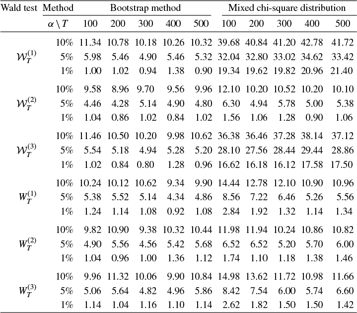
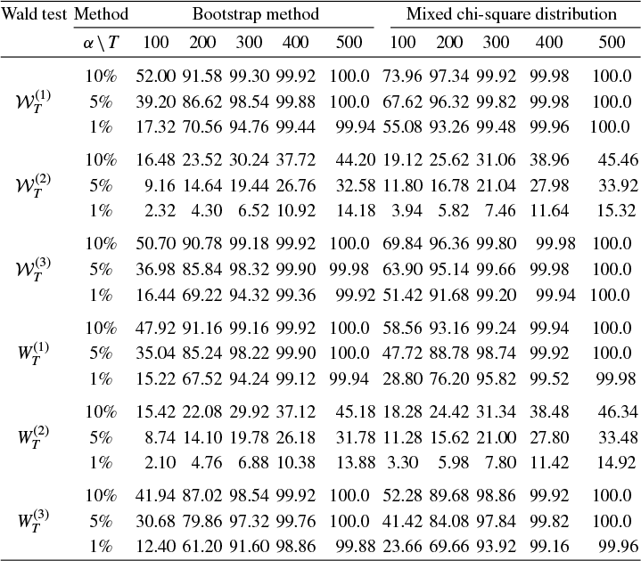
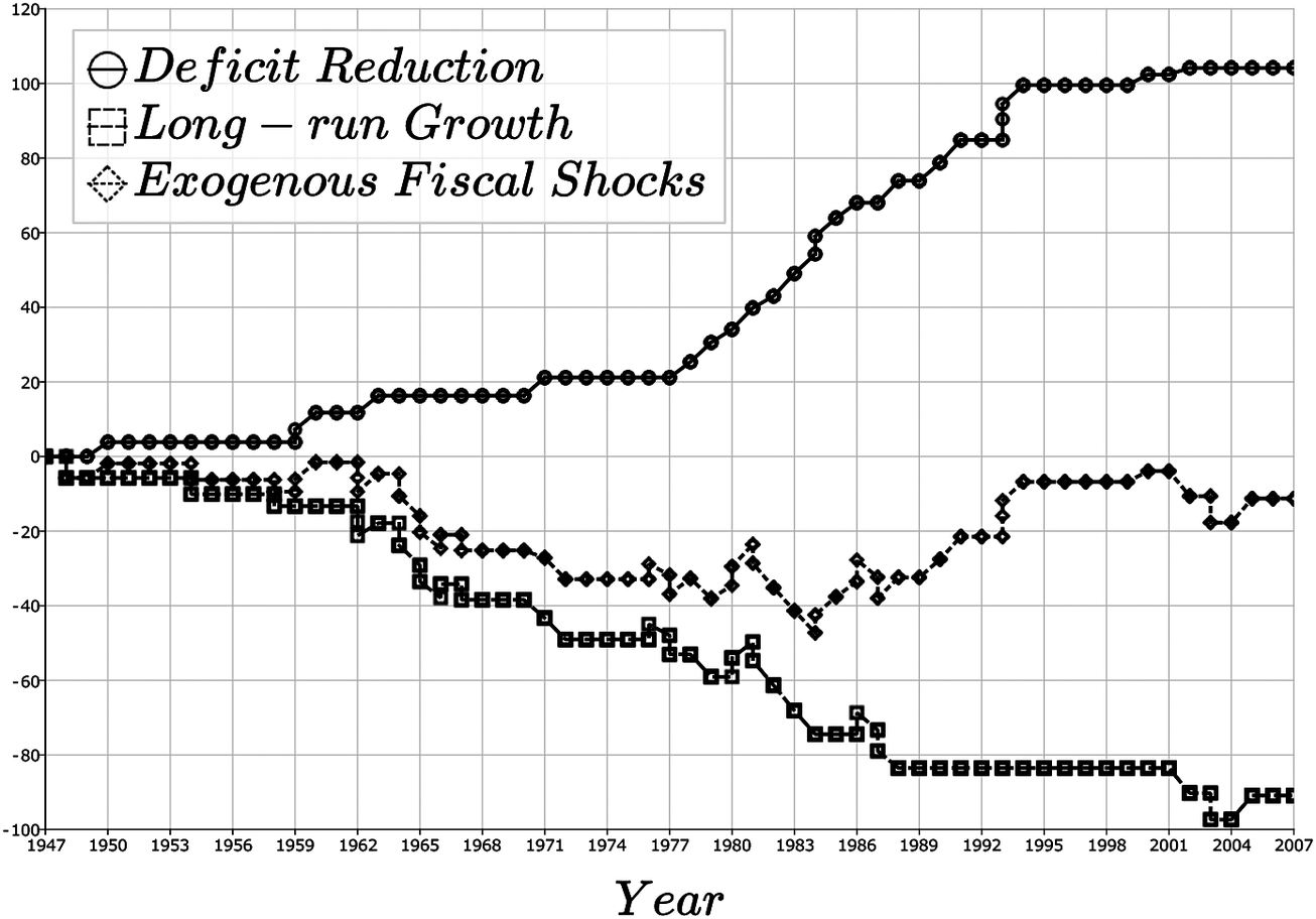
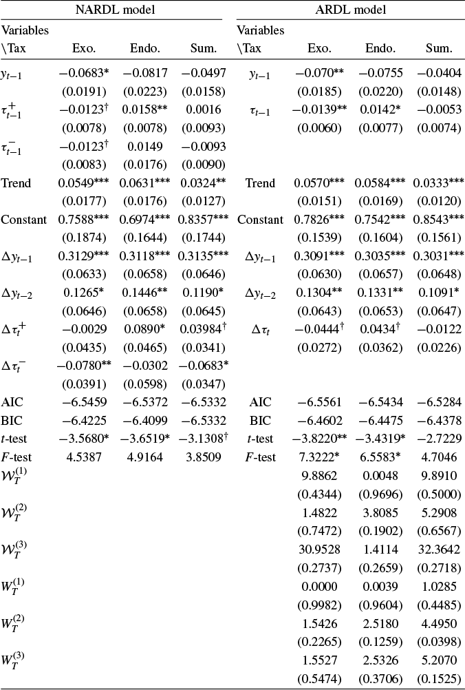
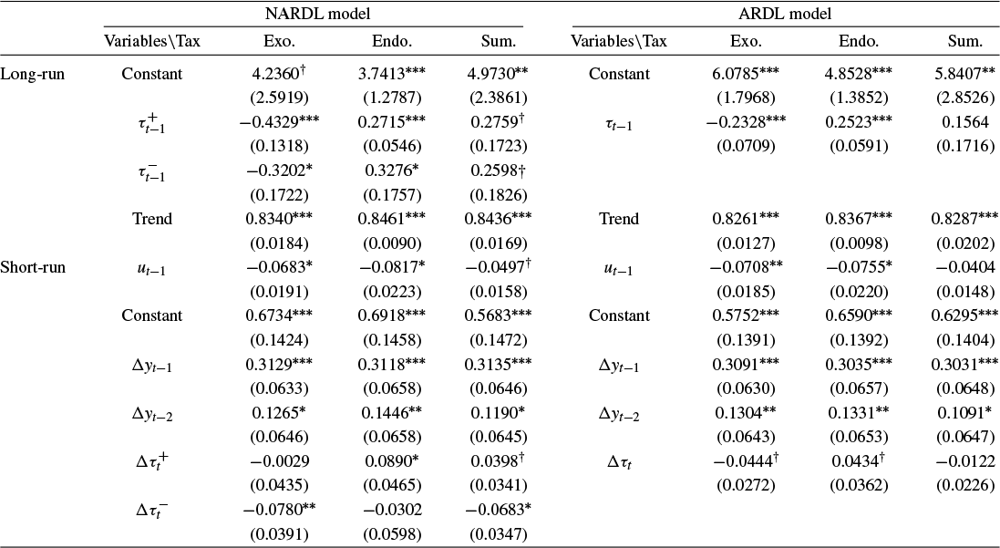


 Open access

