


1 INTRODUCTION
Analysis of data exhibiting persistent regular patterns is important in many empirical studies. For example, a large body of literature is dedicated to the investigation and extraction of periodic or quasi-periodic behavior in macroeconomic, geophysical, and climatic time series. In applications, it is common to make a distinction between cyclicality and seasonality. Seasonal or periodic fluctuations are viewed to be generated by factors, such as the quarter or month of the year, day of the week, etc. As such, seasonality is considered to be of a fixed and, often, of known period. On the other hand, cyclicality refers to oscillations that are determined partly by an exterior impulse which may operate irregularly. Hence, cyclicality is not of fixed period but “[
$\ldots $
 ] takes place within such limits that it is reasonable to speak of an average period [
$\ldots $
 ]”—Frisch (Reference Frisch and K.1933). The lengths of these quasi-cycles typically exceed two years, are not known a priori, and are less clearly identifiable due to the additional variability of their sample ACFs.
In this article, we focus on the estimation theory for the frequency of a cycle. We make no distinction between the terms “seasonality” and “cyclicality” since they have the same spectral characterization, and consider from the outset that the length of an oscillation or cycle is unknown. Correctly establishing this quantity enables the accurate representation of the cyclical patterns characterizing the underlying data and avoids over- or under-parameterizations in model building. This, then, can provide reliable guidance for policy adjustments. Our key objective is to produce a statistical procedure for the estimation of the length of a cycle in an unrestrictive setting. For this purpose, we also introduce a class of semiparametric processes that enables modeling of cyclical behavior in stationary and non-stationary environments.
First, we provide a formal exposition of this new generic class of semiparametric cyclical memory CM
$(\omega ,d)$
 processes and describe its main features. These processes can reproduce random cyclical patterns with a pole at frequency
$\omega $
 on
$[0,\pi ]$
 Footnote
1
and can be stationary or non-stationary as determined by the memory parameter
$d$
 . They are written as

where
$\{Z_{j}\}$
 is an integrated I
$(d)$
 process,
$\{Z_{j}^\prime \}$
 is its independent copy, and
$\mu $
 is an intercept. Parameter
$d$
 in the I
$(d)$
 process
$Z_j$
 can range between 0 and 3/2 and, hence, describes both stationary and non-stationary alternatives, while the spectral density of
$Z_j$
 (pseudo-spectral density in the non-stationary case) has a peak at frequency
$0$
 . This generates a peak at frequency
$\omega $
 in the spectrum
$f_{X}$
 of
$\{X_{j}\}$
 which constitutes the main feature of CM processes and defines the length of the quasi-cycle as
$\lambda =2\pi /\omega $
 . The sharpness of the peak is characterized by the same integration (memory) parameter
$d\in (0, 3/2)$
 as for
$Z_j$
 and it does not vary with
$\omega $
 . Differencing our cyclical process
$X_{t}$
 does not remove persistence when
$\omega \ne 0$
 , even if fractional differencing were to be used, because the peak of the spectrum is not at frequency zero. This has practical implications that will be illustrated in our empirical applications. A special case of CM models arises from the macroeconomic model of Abadir and Talmain (Reference Abadir and Talmain2002) that incorporates the effects of aggregation on the persistence of economic activity variables, as explained in Abadir and Talmain (Reference Abadir, Talmain, A. and Giles2011), hence its relevance in economics (and beyond). Independently, Proietti and Maddanu (Reference Proietti and Maddanu2024) also provide a description of a parametric version of the CM process, see Section 4 below (they call it a sinusoidal waveform process) and discuss its properties and applications but only in the stationary case. For alternative modeling approaches of non-stationary cyclical time series, see, for example, del Barrio Castro, Rodrigues, and Taylor (Reference del Barrio Castro, Rodrigues and Taylor2018, Reference del Barrio Castro, Rodrigues and Taylor2019); del Barrio Castro, Cubadda, and Osborn (Reference del Barrio Castro, Cubadda and Osborn2022), Maddanu (Reference Maddanu2022), and Kang and Marmer (Reference Kang and Marmer2024).
Next, we set up the estimation theory for parameter
$\omega $
 in the CM
$(\omega ,d)$
 model. We estimate
$\omega $
 by the Fourier frequency
$\widehat {\omega }$
 which maximizes the periodogram of cyclical time series
$X_j$
 . Such an estimator is easy to compute. In finite samples, it becomes more precise as the memory parameter
$d$
 increases and, crucially, does not hinge on a particular parametric specification for
$Z_j$
 . We establish
$n^{-1}$
 rate of consistency (
$n$
 being the sample size) for the estimator
$\widehat \omega $
 as well as its asymptotic distribution. Monte Carlo simulations confirm the validity of the asymptotic theory and illustrate its properties in finite samples. They show the location of the pole
$\omega $
 to be confined with high probability (
$>$
 95%) within confidence intervals comprising of up to two Fourier frequencies,
$\widehat {\omega }\pm u_{j}$
 ,
$j=1,2,$
 where
$u_{j}=2\pi j/n$
 , when
$d\geq 0.4$
 . Though the width of these confidence bands is linked to the memory parameter
$d$
 , simulation experiments confirm that for
$d$
 in excess of 0.35 or 0.4 the true pole
$\omega $
 lies within one or two Fourier frequencies around the frequency
$\widehat \omega $
 with high probability (see Section 3).
For modeling cyclical behavior in empirical work, we introduce a parametric auto-regressive cyclically-integrated moving-average ARCIMA(
$p,\omega ,d,q$
 ) model. The ARCIMA model allows parametric modeling of cyclical patterns both in stationary and non-stationary time series. It falls within the class of cyclical memory CM
$(\omega ,d)$
 processes. This model is obtained from the CM
$(\omega ,d)$
 specification (1.1) by setting
$\{Z_{j}\}$
 to be a parametric fractional ARIMA
$(p,d,q)$
 process, with
$d\in (0,3/2)$
 ,

where
$B$
 is the backshift operator, and polynomials
$\phi (B)$
 and
$\theta (B)$
 satisfy the standard assumptions of a stationary ARMA model. The (pseudo-)spectrum of ARIMA process
$Z_j$
 in (1.2) exhibits an infinite peak at zero frequency consistent with the operator
$(1-B)^{d}$
 and memory parameter
$d$
 only. If
$p\neq 0$
 or
$q\neq 0$
 , then the shape of the infinite peak in the spectrum of the ARIMA process
$Z_j$
 at zero frequency is adjusted to reflect the relevant (bounded) spectrum of the ARMA components. The cyclical model (1.1) shifts this peak to the frequency
$\omega $
 in the spectrum of
$X_j$
 which can be estimated using the estimation methods and results established for the CM
$(\omega ,d)$
 model (see Section 3).
Estimation of other parameters of
$Z_j$
 , including
$d\in (0,3/2),$
 is challenging and beyond the scope of this article. Our empirical findings of Section 6 on
$\mathrm {CO}_{2}$
 concentration suggest that, when fitting a stationary ARCIMA model with predetermined cyclical frequencies, as in Proietti and Maddanu (Reference Proietti and Maddanu2024), maximum likelihood estimation can result in over-parameterization and estimates of
$d$
 that hit the upper bound of the stationary region (
$\hat {d}\approx 1/2$
 ). Theoretical results of our article on estimation of
$\omega $
 can be extended easily to the case of multiple poles. However, testing for the existence of cyclical patterns (a pole
$\omega $
 in the spectrum) requires a separate theoretical analysis.
The closest alternative to the stationary version of the above parametric ARCIMA(
$p,\omega ,d,q$
 ) model is the parametric Gegenbauer auto-regressive moving-average (GARMA) model introduced by Andel (Reference Andel1986) and Gray, Zhang, and Woodward (Reference Gray, Zhang and Woodward1989, Reference Gray, Zhang and Woodward1994). This emerged from the earlier idea of Granger and Joyeux (Reference Granger and Joyeux1980) and Hosking (Reference Hosking1981) to use a generalization of a fractionally differenced model to allow for seasonality in a time-series process. The GARMA model for seasonal time-series process
$\{X_{j}\}$
 is given by

where
$0\leq \omega \leq \pi $
 ,
$|d|<1/2$
 ,
$\{\zeta _{j}\}$
 is a white noise
$(0,\sigma _{\zeta }^{2})$
 sequence, and
$\phi (B)$
 and
$\theta (B)$
 are as before. The GARMA model with memory parameter
$0<d <1/2$
 allows the modeling of long-term persistence and quasi-periodic behavior, and its correlation function resembles a superposition of hyperbolically damped sine waves. The spectral density of such time series again has a pole at
$\omega $
 on
$[0,\pi ]$
 .
While the ARCIMA specification falls within the class of our proposed cyclical memory CM
$(\omega ,d)$
 processes, GARMA and CM models are not nested. Hence, the GARMA model does not share some of ARCIMA’s benefits, including the ease of simulation and the uniform persistency over
$\omega $
 (see Section 2). For example, unlike ARCIMA, simulation of a Gaussian GARMA process using algorithm of Davies and Harte (Reference Davies and Harte1987) is not straightforward. This algorithm requires knowledge of the autocovariance function, which for a GARMA
$(0,d,0)$
 process is rather complicated, and not available for a GARMA model with multiple poles. Further, for a given
$d$
 , the sharpness of peak in the spectrum of ARCIMA process is uniform over the location of the peak,
$\omega $
 , while for GARMA, it doubles to
$2d$
 at
$\omega =0$
 (see Section 4). Regarding estimation, focusing solely on the estimation of
$\omega $
 , Hidalgo and Soulier (Reference Hidalgo and Soulier2004) obtain a consistency rate
$n^{-1+\epsilon }$
 for a Gaussian GARMA model, which is lower than our consistency rate of
$n^{-1}$
 for CM
$(\omega ,d)$
 models, and do not establish the asymptotic distribution of
$\widehat \omega $
 . Overall, when
$\omega $
 is unknown, parametric estimation of the GARMA model becomes significantly harder (see Giraitis, Hildago, and Robinson, Reference Giraitis, Hildago and Robinson2001).
Our empirical illustration covers three examples from macroeconomics and climate science. We investigate the presence of persistent regular patterns (periodic and quasi-periodic) in U.S. nominal GDP over the period Q1-1956 to Q4-2019, U.S. real industrial production (IP) over the period August 1977 to December 2019, and
$\mathrm {CO}_{2}$
 concentration over the period May 1978 to December 2020. In all cases, it is evident that well-defined peaks in the periodogram are indicative of persistent cyclical patterns, while less pronounced/ambiguous peaks reflect reduced evidence for cyclical structure and require further investigation using complementary tools.
The article is organized as follows. Section 2 outlines the formal definition of the semiparametric class CM
$(\omega ,d)$
 of cyclical models, together with their autocovariance and spectral density properties. Section 3 presents theoretical results for estimation of the location parameter
$\omega $
 , based on the estimator
$\widehat {\omega }$
 for CM
$(\omega ,d)$
 processes. Section 4 introduces the parametric ARCIMA model. Section 5 reports Monte Carlo simulation results, while Section 6 presents empirical examples from macroeconomics and climate research. Proofs and additional simulation results are provided in Appendixes A–C of the Supplementary Material.
2 SEMIPARAMETRIC CYCLICAL–MEMORY MODEL
In this section, we introduce a class of semiparametric CM(
$\omega ,d$
 ) cyclical–memory processes that enable the modeling of regular cyclical patterns in stationary and non-stationary time series. These models are characterized by two parameters,
$\omega $
 and
$d$
 , for cycle and memory, respectively. They have spectral density (pseudo-spectral density in the non-stationary case) that is unbounded at frequency
$\omega \in (0,\pi )$
 and the sharpness of the peak is defined by the memory parameter
$d\in (0,3/2)$
 . This domain of
$d$
 covers most time series of practical interest. It can be extended to
$d>3/2$
 in the same way that we extend the stationary I
$(d)$
 ,
$d\in (0,1/2)$
 process to
$d\in (1/2,3/2)$
 in Definition 2.1 below.
The precise definition of the semiparametric CM
$(\omega ,d)$
 model with a pole at frequency
$\omega \in (0,\pi )$
 in the spectrum uses a semiparametric integrated I
$(d)$
 process, the spectral density of which has a pole at zero frequency,
$\omega =0$
 .
Definition 2.1.
(a)
$\{Z_{j}\}$
 is said to be an
$\mathrm{I}(d)$
 process with
$|d|<1/2$
 if:
(i)
$\{Z_j, \,\, j\in {\mathbb {Z}}\}$
 is a stationary linear process of the form

where
$\{\zeta _{j}\} $
 is an i.i.d. sequence with
$\mathrm {E}\zeta _j=0$
 ,
$\mathrm {E}\zeta _j^2=\sigma _{\zeta }^{2}$
 , and
$\mathrm {E}\zeta _j^4<\infty $
 .
(ii) The spectral density function of
$\{Z_j\}$
 can be written as

where
$g>0$
 is a continuous function bounded away from
$0$
 and
$\infty $
 .
(iii) The covariance function
$\gamma _{Z}(k)=\mathrm {cov}(Z_{k},Z_{0})=\int _{-\pi }^\pi \mathrm{e}^{\mathrm {i} ku}f_Z(u)du $
 and the coefficients in
$a_k$
 in (2.1) satisfy

(b) A process
$\{Z_{j}\}$
 is said to be an I
$(d)$
 with
$d\in (1/2,3/2)$
 process if
${\nabla Z_{j}=Z_{j}-Z_{j-1}}$
 is an I
$(d-1)$
 process as defined in part (a). We assume that
${Z_0=O_p(1)}$
 . In this case,
$d-1\in (-1/2,1/2)$
 .
For
$0<d<1/2$
 , the process
$\{Z_{j}\}$
 is stationary with long memory, and its spectral density
$f_{Z}$
 is unbounded at the zero frequency:
$f_{Z}(u)\sim c|u|^{-2d}$
 as
$u\rightarrow 0 $
 . For
$1/2<d\leq 1$
 , an analogous property holds for the pseudo-spectral density
$f_{Z}$
 (see (2.11)).
Remark 2.1. Parametric stationary ARIMA(
$p,d,q$
 ) processes are I
$(d)$
 processes and satisfy Assumption 3 below (see Chapters 3 and 7 and Remark 6.2.2 in Giraitis, Koul, and Surgailis, Reference Giraitis, Koul and Surgailis2012). The condition
$\sum _{k=0}^{\infty }a_{k}=0$
 for
$d<0$
 is aligned with (2.2), since
$2\pi f(0)=\sum _{k=-\infty }^{\infty }\gamma _{Z}(k)=\sigma _{\zeta }^{2}(\sum _{k=0}^{\infty }a_{k})^{2}=0$
 .
We can now introduce a new class of semiparametric cyclical–memory processes, denoted CM
$(\omega ,d)$
 , defined as follows.
Definition 2.2. A process
$\{X_{j}\},\,j\in {\mathbb {Z}},$
 is said to be a CM
$(\omega ,d)$
 cyclical–memory process with parameters
$\omega \in (0,\,\pi )$
 and
$ d\in (0,3/2)\backslash \{1/2\}$
 , if it can be written as

where
$\{Z_{j}\}$
 is an I
$(d)$
 process,
$\{Z_{j}^{\prime }\}$
 is an independent copy of
$\{Z_{j}\}$
 , and
$\mu $
 is an intercept.
The next theorem provides the main properties of a stationary CM
$(\omega ,d)$
 model with
$0<d<1/2$
 . It shows that these processes are covariance stationary, their autocovariance functions decay as hyperbolically damped sine waves, and their spectral densities have an infinite peak at frequency
$\omega $
 , remaining bounded and continuous at all other frequencies on the spectrum.
We assume that
$f_{Z}$
 in (2.2) is extended to the real line
${{ \mathbb {R}}}$
 with period
$2\pi $
 .
Theorem 2.1. Suppose that
$0<\omega <\pi $
 and
$0<d<1/2$
 . Then the CM
$(\omega ,d)$
 process
$\{X_{j}\}$
 in (2.4) has the following properties:
(i)
$\{X_{j}\}$
 is covariance stationary, with autocovariance function
$\gamma _{X}$
 and spectral density
$f_{X}$
 given by

where
$g_{X}(u)$
 is a continuous even function bounded away from zero and infinity.
(ii) Let
$a_k, \zeta _k$
 be as in (2.1), and let
$\{\zeta _{k}^{\prime }\}$
 be an independent copy of
$\{\zeta _{k}\}$
 . Then


where

In (2.6), for each
$j$
 ,
$\{\xi _{j,k}, \,k\in \mathbb {Z}\}$
 is an i.i.d.
$(0, \sigma ^2_\zeta )$
 sequence. In (2.7), the sequences
$\{\eta _{k}\}$
 and
$\{\eta ^*_{k}\}$
 are mutually uncorrelated sequences of independent variables with
$ \mathrm {E}\eta _{k}=\mathrm {E}\eta _{k}^*=0$
 and
$ \mathrm {E}\eta _{k}^2=\mathrm {E}\eta _{k}^{*2}=\mathrm {E}\zeta _{k}^2=\sigma _\zeta ^2$
 .
Proof. See Appendix A of the Supplementary Material. Representation (2.7) extends Proposition 1 in Proietti and Maddanu (Reference Proietti and Maddanu2024), originally established for Gaussian processes, to the case of non-Gaussian cyclical–memory processes.
For a non-stationary cyclical process
$X_j \sim $
 CM
$(\omega ,d)$
 ,
$ d \in (1/2, 3/2)$
 , cyclical patterns can be captured by the sample covariance function
$\widehat {\gamma }_{X}(k)$
 and the periodogram
$I_{X}(u)$
 :

Theorem 2.2 shows that (on average)
$\widehat {\gamma }_{X}(k)$
 exhibits the same cyclical behavior as
$\gamma _{X}(k)$
 in the stationary case in (2.5).
Theorem 2.2. Let
$0<\omega <\pi $
 and
$d\in (1/2,3/2)$
 . Suppose that
$ X_{j}\sim $
 CM
$(\omega ,d)$
 and that
$Z_{j}\sim $
 I
$(d)$
 with
$\mathrm {E} (Z_{j})=0$
 . Then,

Proof. See Appendix A of the Supplementary Material.
In the stationary case, when
$d\in (0,1/2)$
 , the spectral densities
$ f_{Z}(u),f_{X}(u)$
 and their empirical counterparts (the periodograms
$ I_{Z}(u),I_{X}(u)$
 ) are related as follows: as
$n\rightarrow \infty $
 ,

Theorem 3.1 in Section 3 shows that (2.9) remains valid for non-stationary CM
$(\omega ,d)$
 processes with
$d\in (1/2,1]$
 , provided that the spectral densities are replaced by pseudo-spectral densities:

where
$f_{Z}(u)$
 is extended periodically to
${\mathbb {R}}$
 . These functions are not integrable. Notice that
$f_{\nabla Z}(0)=0$
 for
$d\in (1/2,1)$
 . These pseudo-spectral densities exhibit the same pattern of cyclical behavior as for
$\{Z_{j}\}$
 ,
$\{X_{j}\}$
 in the stationary case:

where
$g_{Z}(u)$
 and
$g_{X}(u)$
 are continuous functions bounded away from zero and infinity.
3 ESTIMATION OF
$ \omega $


In this section, we discuss the estimation of the parameter
$\omega $
 of a cyclical process
$X_{j}\sim $
 CM
$(\omega ,d)$
 when
$0<d<3/2$
 and
$d\ne 1/2$
 . The estimation of
$\omega $
 will be based on the periodogram:

where
$w_{X}(u)$
 is the discrete Fourier transform (DFT), both based on the sample
$X_{1},\ldots ,X_{n}$
 .
For
$d\in (0, 1/2)$
 , the spectral density
$ f_{X}(u),\,\,u\in \Pi , $
 of a stationary cyclical process
$\{X_{j}\}$
 has an infinite peak at the frequencies
$u=\pm \omega $
 . For
$d\in (1/2,1]$
 , the cyclical times series
$\{X_{j}\}$
 is non-stationary, and its pseudo-spectral density
$ f_{X}(u)$
 , defined in (2.10), also has an infinite peak at frequencies
$\pm \omega $
 (see Theorem 3.2). Although the periodogram
$I_{X}(u)$
 is only a mean consistent estimator of
$f_{X}(u)$
 at the continuity points
$u\in \Pi \backslash \{\pm \omega \}$
 , one can expect that the location of the maximum of the periodogram will converge to the location of the maximum of
$f_{X}(u)$
 ,
$0\le u\le \pi $
 , that is,
$\omega $
 , at a fast rate. This is confirmed by Theorem 3.3 below.
We define the estimator
$\widehat {\omega }$
 of
$ \omega $
 as the maximizer of the periodogram:

over the set of Fourier frequencies
$u_{j}=2\pi j/n$
 ,
$j=1,\ldots , \widetilde {n} :=\lfloor n/2\rfloor -1$
 . Note that
$u_{ \widetilde {n}}\sim \pi $
 .
This estimator was introduced by Hidalgo and Soulier (Reference Hidalgo and Soulier2004) for the estimation of
$\omega $
 in a stationary Gaussian GARMA model. In their Theorem 2, they establish the consistency rate
$\widehat \omega - \omega =O_{p}(n^{-1+\epsilon })$
 for any
$\epsilon>0$
 and abstain from deriving the asymptotic distribution. By comparison, we establish the consistency rate
$O_{p}(n^{-1})$
 in estimation of
$\omega $
 for both stationary and non-stationary CM
$(\omega ,d)$
 processes (see Theorem 3.2 below). Furthermore, in Theorem 3.3, we derive the asymptotic distribution for
$\widehat {\omega }$
 .
For simplicity, in the next theorems, we assume that the pole
$\omega $
 is at a Fourier frequency
$\omega =u_{k_{0}}$
 , where
$k_{0}:=k(n)$
 is an integer. and suppose that

Establishing the consistency rate and asymptotic distribution for
$\widehat { \omega }$
 requires additional assumptions on the I
$(d)$
 process
$\{Z_{j}\}$
 that appear in the definition (2.4) of the CM
$(\omega ,d)$
 process
$\{X_{j}\}$
 .
By Definition 2.1(i), for
$0<d<1/2$
 ,
$Z_{j}=\sum _{k=0}^{\infty }a_{k}\zeta _{j-k}$
 is a stationary linear process. For
$1/2<d<3/2$
 ,
$\nabla Z_{j}=\sum _{k=0}^{\infty }a_{k}^{\prime }\zeta _{j-k}$
 also can be written as a stationary linear process. We impose the following additional assumptions on their transfer functions:

Assumption 1. I
$(d)$
 process
$\{Z_{j}\}$
 in (2.4) has the following properties:
For
$0<d<1/2$
 , assume that
$\mathrm {E}|\zeta _{j}|^{q}<\infty $
 for some
$q>1/4d$
 . Moreover,


where
$C$
 does not depend on
$u\in \Pi $
 .
We consider the estimation of the parameter
$\omega $
 by the same estimator
$\widehat \omega $
 both when the cyclical CM
$(\omega ,d)$
 process
$\{X_j\}$
 is stationary and non-stationary. The following theorem provides insights on why, for a non-stationary cyclical process, the periodogram also tends to peak around the frequency
$\omega $
 . It relates the periodograms
$I_{X}, I_Z$
 to the pseudo-spectral densities
$f_{X}, \,f_Z$
 given in (2.10). Recall that
$f_X$
 has an infinite pole at frequency
$\omega $
 , while
$f_Z$
 has one at frequency
$0$
 .
Theorem 3.1. Let
$0<\omega <\pi $
 and
$d\in (1/2,1]$
 . Suppose that
$X_j\sim $
 CM
$(\omega ,d)$
 and
$Z_{j}\sim \mathrm{I}(d)$
 satisfy Assumption 1. Then, for any
$\epsilon>0$
 , as
$n\rightarrow \infty $
 ,

Proof. See Appendix A of the Supplementary Material.
Theorem 3.2. Let
$0<\omega <\pi $
 ,
$d\in (0,3/2),$
 and
$d\neq 1/2$
 . Assume that the CM
$(\omega ,d)$
 process
$\{X_{j}\}$
 satisfies Assumption 1. Then, the estimator
$\widehat {\omega }$
 of
$\omega $
 is
$n$
 -consistent:

Proof. See Appendix A of the Supplementary Material.
Notice that the consistency result (3.8) holds both for stationary CM
$(\omega ,d)$
 process
$\{X_{j}\}$
 when
$0<d<1/2$
 and for non-stationary process when
$1/2<d<3/2$
 .
The next theorem establishes the asymptotic distribution of the estimate
$\widehat {\omega }$
 . To describe the limit distribution, write
$\widehat {\omega }=u_{\widehat {k}}=2\pi \widehat {k} /n$
 , where
$\widehat {k}$
 is the number of the Fourier frequency that maximizes the periodogram.
Theorem 3.3. Assume that the CM
$(\omega ,d)$
 process
$\{X_{j}\}$
 satisfies the assumptions of Theorem 3.2 and that (3.2) holds. Then, for any
$L\geq 1$
 ,

where the random variables
$\tau _{d}(k)$
 ,
$k\in {\mathbb {Z}}$
 , have a known distribution which depends only on
$d$
 and
$k$
 .
Proof. See Appendix A of the Supplementary Material.
Theorem 3.3 establishes the existence of the limit distribution of the estimator
$\widehat {\omega }$
 providing a basis for constructing confidence intervals for
$\omega $
 . Similarly to the normalized periodograms of an ARFIMA process when
$d\in (0,1/2)$
 , see, for example, Hurvich and Beltrao (Reference Hurvich and Beltrao1993), the variables
$\tau _d(k)$
 are neither independent nor identically distributed. They are known and form a sequence of dependent random variables, the definition of which involves Gaussian sequences determined solely by the parameter
$d$
 . They can be simulated, provided that
$d$
 is known, and do not depend on
$\omega $
 or on any short-run dynamic parameters. Due to their involved structure, we do not reproduce their definitions here. Instead, we refer the reader to equations (A.41) and (A.48) in the Supplementary Material.
Building Confidence Intervals. In this article, we focus exclusively on the estimation of the parameter
$\omega $
 when
$d$
 is unknown. Theorem 3.3 provides the basis for constructing conservative confidence intervals for
$\omega $
 as follows.
The researcher selects the desired coverage probability, for example,
$\alpha = 0.90$
 or
$0.95$
 . The confidence interval for
$\omega $
 is then given by

For a given
$m$
 , the researcher may wish to determine the minimal level of persistence
$d\ge d_{0,\alpha }^{(m)}$
 required for the interval to cover
$\omega $
 with probability at least
$\alpha $
 . According to Theorem 3.3, these values do not depend on
$\omega $
 , but they do depend on
$m$
 .
Simulation-based methods allow us to determine the values
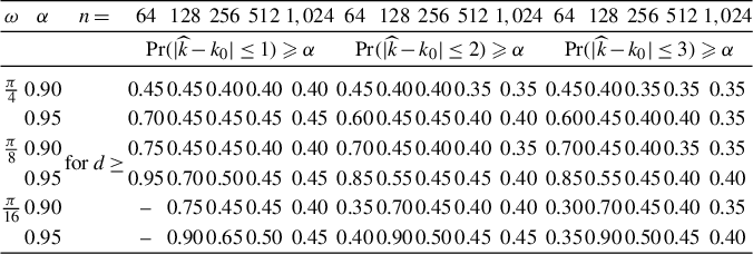
$d_{0,\alpha }^{(m)}$
 for a range of sample sizes and values of
$\omega $
 (see Table 2 in Section 5). The results indicate that
$d_{0,\alpha }^{(m)}$
 is approximately independent of
$\omega $
 and
$n$
 for sample sizes
$n \ge 128$
 . Table 2 provides guidance on the coverage rate of the interval
$[\widehat \omega - u_m, \widehat \omega + u_m]$
 for selected values
$m = 1,2,3$
 , given a user-specified lower bound for the persistence parameter
$d$
 .
The width of the confidence interval is determined by the Fourier frequencies
$u_m$
 . For example, to achieve
$90\%$
 coverage of
$\omega $
 by the interval

that is, when
$\omega $
 lies within two Fourier frequencies of
$\widehat {\omega }$
 , the minimal persistence level is approximately
$d_{0,\alpha }^{(m)} \approx 0.4$
 for sample sizes
$n \ge 128$
 .
Inclusion of short-run dynamics in the ARCIMA model does not adversely affect coverage, since the spectral peak that arises from the memory parameter
$d$
 dominates the contribution from shorter memory dynamics (see Figure 6 in the Supplementary Material).
Remark 3.1. In this article, we discuss cyclical processes CM
$(\omega ,d)$
 that have a single pole in their spectrum. It can be shown that the sum
$X_{j}=X_{j}(\omega _{1},d_{1})+\cdots +X_{j}(\omega _{m},d_{m})$
 of
$m$
 -mutually independent CM
$(\omega ,d)$
 processes with parameters
$ (\omega _{1},d_{1}),\dots ,(\omega _{m},d_{m})$
 produces a time series
$\{X_{j}\}$
 with
$m$
 peaks at frequencies
$\omega _{1},\ldots ,\omega _{m}$
 in its spectrum. We conjecture that these frequencies can be estimated using the frequencies
$ \widehat {\omega }_{1},$
 …,
$\widehat {\omega }_{m}$
 of the local maxima of the periodogram. These estimators have
$n^{-1}$
 rate of convergence and a similar asymptotic theory should hold as for
$m=1$
 discussed in this article.
Remark 3.2. Definition 2.2 introduces a stationary cyclical process
$X_j$
 in (2.4) that has nonzero mean
$\mu $
 . The periodogram
$I_X(u_k)$
 at Fourier frequencies
$u_k, k=1,\ldots , n-1,$
 is shift invariant, that is,
$I_X(u_k)=I_{X+\mu }(u_k)$
 for any
$\mu $
 . Therefore, it suffices to prove the validity of the results of this article for
$X_j$
 with
$\mu =0$
 :

Allowing for a deterministic time-varying component
$\mu _j = a\cos (\omega j) + b\sin (\omega j),\, j\in { \mathbb {Z}}, $
 in Definition 2.2 is an interesting extension for future work.
Remark 3.3. Our theoretical results are derived under the assumption that the pole
$\omega $
 in Definition 2.2 coincides with a Fourier frequency, that is,
$\omega =u_{k_{0}}$
 . This condition can be relaxed, though such an extension would require additional technical elaboration. In the simulation study of Section 5, we assess the performance of our estimator of
$\omega $
 both under the baseline case
$\omega =u_{k_{0}}$
 and in the non-Fourier frequency case,
$\omega =u_{k_{0}}+u_{1}/2$
 . The results are nearly identical in both settings (see Tables 2 and 3 in Section 5, and Tables 4 and 5 in the Supplementary Material).
4 PARAMETRIC CYCLICALLY-INTEGRATED ARCIMA MODEL
There are several stationary parametric models that allow for the estimation of cyclical patterns in the data. Among these are the ARUMA model by Anderson (Reference Anderson1979), the GARMA model by Gray et al. (Reference Gray, Zhang and Woodward1989, Reference Gray, Zhang and Woodward1994) and Giraitis and Leipus (Reference Giraitis and Leipus1995), and the sinusoidal waveform model by Proietti and Maddanu (Reference Proietti and Maddanu2024). Separately, Abadir, Distaso, and Giraitis (Reference Abadir, Distaso and Giraitis2011) consider a stationary and non-stationary I(
$d$
 ) model with trend and non-random cycles in the mean of known periodicity.
In this section, we introduce ARCIMA as an example of a parametric model that satisfies our definition of a cyclical CM
$(\omega ,d)$
 process. By construction, it imposes a parametric fractional ARIMA structure on I
$(d)$
 process
$Z_j$
 in the generating equation (2.4) of CM
$(\omega ,d)$
 model, which shifts the pole of the spectral density of the fractional ARIMA process from zero to frequency
$\omega \in (0,\pi )$
 . The ARCIMA model makes use of the well-known properties of the ARIMA(
$p,d,q$
 ) process in (1.2), which allow for an easy simulation of a Gaussian ARCIMA using the Davies and Harte (Reference Davies and Harte1987) algorithm.
Definition 4.1.
Let
$\omega \in (0,\,\pi )$
 ,
$d\in (0,3/2)\backslash \mathrm {\{1/2\}}$
 . An ARCIMA
$(p,\omega ,d,q)$
 process
$\{X_{j}\}$
 is a CM
$(\omega ,d)$
 process in (2.4) generated by an I(
$d$
 ) process
$Z_j\sim $
 ARIMA
$(p,d,q)$
 .
Definition 4.2. The CI
$(\omega ,d)$
 model is defined as the special case of the ARCIMA
$(p,\omega ,d,q)$
 model with
$p=q=0$
 , that is, an ARCIMA
$(0,\omega ,d,0)$
 process.
Remark 4.1. For
$0<d<1/2$
 , the CI
$(\omega , d)$
 process is covariance stationary. Its autocovariance function exhibits damped oscillations and decays to zero, while its spectral density has an infinite peak at frequency
$\omega $
 :


where

Here,
$f_{Z}(u)$
 is the spectral density of an ARIMA
$(0,d,0)$
 process, and
${g}_X(u)=|u-\omega |^{2d}(f_{Z}(u-\omega )+f_{Z}(u+\omega ))/2$
 is a Lipschitz
$\Lambda _{2d}$
 function with parameter
$2d$
 . This holds because both
$ |u-\omega |^{2d}f_{Z}(u-\omega )$
 and
$f_{Z}(u+\omega )$
 are differentiable functions on
$[0,\,\pi ]$
 and
$|u-\omega |^{2d}$
 belongs to
$\Lambda _{2d}$
 .
Similar asymptotic properties hold for the parametric autocorrelation function (8.1) in Abadir and Talmain (Reference Abadir, Talmain, A. and Giles2011) and the corresponding spectrum in their Definition 8.1.
Remark 4.2. Notably, the ARCIMA and GARMA classes of cyclical models are not nested. Consider a stationary ARCIMA
$(0,\omega ,d,0)$
 process
$X_j$
 as in (2.4), generated by an ARFIMA(
$0,d,0$
 ) process
$Z_j$
 with
$|d|<1/2$
 . Its spectral density is given by

By contrast, the GARMA(
$0,d,0$
 ) process has spectral density

It is straightforward to verify that

which shows that GARMA and ARCIMA models are not nested.
Equality (4.3) demonstrates that the cyclical memory of a stationary ARCIMA time series
$X_j$
 cannot be removed by GARMA-type fractional differencing. The filtered series

has spectral density

which coincides with the spectral density
$f_X(-d,u)$
 of a stationary cyclical ARCIMA process with memory parameter
$-d$
 .
It is important to point out the connection between (4.3) and Proposition 3(ii) in Proietti and Maddanu (Reference Proietti and Maddanu2024). Their result establishes the relationship between ARCIMA and GARMA representations as in (2.7) for Gaussian processes, and this relation follows directly from the equality of the spectral densities in (4.3).
In terms of the GARMA model, the algorithm by Davies and Harte (Reference Davies and Harte1987) allows the simulation of a Gaussian version of the process, but requires knowledge of its autocovariance function, which for a GARMA
$(0,d,0)$
 process is rather complicated, and not available for models with multiple poles. Further, the sharpness of the spectral peak of the GARMA model is not uniform over the location of the peak,
$\omega $
 , and the memory parameter
$d$
 is doubled to
$2d$
 when
$\omega \rightarrow 0$
 . Given that in many applications
$\omega $
 may be close to zero, this complicates the use of the GARMA model in empirical studies.
The generalized harmonically weighted cyclical process (GHW) introduced by Maddanu (Reference Maddanu2022) also generates peaks in the spectrum and allows for non-stationarity. This model does not include a long-memory parameter, nor does it require its estimation; however, the persistence of the GHW process again varies with the frequency parameter
$\omega $
 . The GHW process is universally less persistent than the GARMA process, regardless of the value of
$d \in (0,1)$
 . The AR
$(2)$
 model with complex conjugate characteristic roots, widely used in macroeconomics, can also produce sharp finite spectral peaks at the frequency
$\omega $
 when the process is in the near-unit root region. Estimation of
$\omega $
 under either specification is challenging and requires separate investigation. Further work is also needed to develop specification tests capable of distinguishing the ARCIMA model from competing cyclical models. For alternative approaches to modeling cyclical persistence, see del Barrio Castro et al. (Reference del Barrio Castro and Osborn2024).
On the contrary, the ARCIMA model makes use of the benefits of the ARIMA framework and is much easier to simulate using the Davies and Harte (Reference Davies and Harte1987) algorithm. For the stationary ARIMA(
$1,d,0$
 ) model, the autocovariance function was derived by Hosking (Reference Hosking1981), and for the ARIMA(
$p,d,q$
 ) model, explicit formulas can be found in Sowell (Reference Sowell1992). Importantly, the persistence or sharpness of the peak in the spectrum in this specification does not vary with
$\omega $
 .
Estimation of the remaining parameters of the ARCIMA
$(p,\omega ,d,q)$
 model is a challenging problem. Proietti and Maddanu (Reference Proietti and Maddanu2024) introduce a maximum likelihood approach for estimating a stationary Gaussian ARCIMA model when the cyclical parameter (frequency
$\omega $
 ) is known. Implementation of this approach requires caution, since misidentification of the pole frequency
$\omega $
 may result in over-parameterization, in which case the MLE procedure is not applicable. Moreover, for non-stationary ARCIMA models with
$d>1/2$
 , the estimator of the memory parameter often tends to hit the upper bound of the stationarity region, that is,
$\widehat {d} \approx 1/2$
 . Parametric Whittle estimation of a stationary GARMA model when the frequency
$\omega $
 of an infinite spectral peak is unknown was investigated in Giraitis et al. (Reference Giraitis, Hildago and Robinson2001). Alternatively, Arteche (Reference Arteche2020) introduced an exact local Whittle estimation method for GARMA models (both stationary and non-stationary) when the frequency
$\omega $
 of the spectral pole is known.
We conjecture that the same asymptotic theory established in this article also holds for the estimator
$\widehat \omega $
 of the pole location
$\omega $
 under a general GARMA specification. However, in this case, the variables
$\tau _d(k)$
 ,
$k \in \mathbb {Z}$
 , appearing in the limit distribution of
$\widehat \omega $
 in Theorem 3.3, would need to be slightly modified. A formal derivation of this extension is currently work in progress.
It is worth noting that consistent estimation of
$d$
 , though desired, is not necessary for the purpose of recovering
$\omega $
 . The confidence intervals provided in this article are conservative. Hence, so long as
$\widehat {d}\geq 0.35,$
 we can be at least
$90\%$
 confident that
$\omega $
 lies within two Fourier frequencies of the true pole (see Table 2). The estimation methods proposed in Proietti and Maddanu (Reference Proietti and Maddanu2024) and Arteche (Reference Arteche2020) can give some indication of the value of
$d$
 of a Gaussian ARCIMA process when
$\omega $
 is known. An estimation procedure for the ARCIMA
$(p,\omega ,d,q)$
 model (both stationary and non-stationary) under unknown
$\omega $
 is being developed and it does not reduce to a straightforward generalization of Arteche (Reference Arteche2020).
5 MONTE CARLO SIMULATIONS
In this section, we study the finite sample properties of our estimator
$\widehat \omega $
 of the location of the cyclicality parameter
$\omega $
 given in (3.1).
5.1 Coverage Rates under CI(
$ \omega ,d$
)

First, we evaluate the precision of estimation of
$\omega =u_{k_{0}}$
 by
$ \widehat {\omega }=u_{\widehat {k}}$
 and its relation to the memory parameter
$ d$
 . We compute the coverage rates for confidence intervals
$\widehat {\omega } \pm u_{m}$
 ,

the probability that
$\omega $
 is within one, two, or three Fourier frequencies of
$\widehat {\omega }$
 . As
$n\rightarrow \infty $
 , these probabilities converge to the limit coverage probabilities described by (3.9) of Theorem 3.3.
We generate
$2,000$
 samples of the parametric Gaussian CI(
$\omega ,d$
 ) process (equivalently, ARCIMA(
$0,\omega ,d,0$
 )), as defined in Section 4, with parameters
$\omega =\left \{ \frac {\pi }{4},\frac {\pi }{8},\frac {\pi }{16}, \frac {\pi }{32}\right \} $
 ,
$d=\left \{ 1.00,0.50,0.45,0.30\right \} $
 , and for sample sizes
$n=\left \{ 64,128,256,512,1,\!024\right \}, $
 using the Davies and Harte (Reference Davies and Harte1987) algorithm. Notice that such
$\omega $
 can be written as
$\omega =u_{k_{0}}$
 for some integer
$k_{0}$
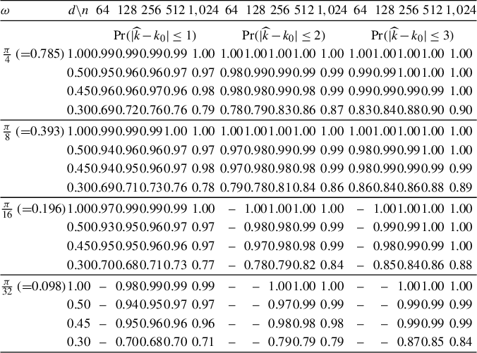
 as required in Theorem 3.3. Table 1 shows the rate at which the true pole
$\omega $
 (location of peak in spectrum) falls within one, two, or three Fourier frequencies from the estimated pole
$\widehat \omega $
 , see (3.1), for the values of
$\omega $
 ,
$d,$
 and
$n$
 considered. It is clear that the coverage remains remarkably stable across
$\omega $
 even when it approaches zero, for sample sizes
$n\geq 64$
 . The coverage rate depends on
$d$
 and slightly drops when
$d$
 decreases to
$0.3$
 . Otherwise, for
$d\geq 0.45$
 , the interval
$(\widehat {\omega }-u_{1},\,\widehat {\omega } +u_{1})$
 produces
$\geq $
 95% coverage for
$\omega $
 . The stability of this (conservative) coverage rate suggests that, in practice, a prominent peak in the periodogram which represents cyclical patterns with memory parameter
$d\ge 0.35$
 can be viewed as a very accurate estimate of
$\omega $
 irrespective where it is located. This experiment confirms the theoretical findings of Theorem 3.3.
Coverage rate for confidence intervals
$\widehat { \omega } \pm u_m$
 of
$ \omega $
 for
$m=1,2,3$
 .

Table 1 Long description
The table is organized with a header row containing omega, d forward slash n, and sample sizes n equals 64, 128, 256, 512, and 1,024 repeated across three main probability categories.
Row 1 Header: The three main categories are P r (absolute value of k-hat minus k sub 0 is less than or equal to 1), P r (absolute value of k-hat minus k sub 0 is less than or equal to 2), and P r (absolute value of k-hat minus k sub 0 is less than or equal to 3).
Data Rows by Omega:
- For omega equals pi over 4 (0.785): Coverage rates for d forward slash n values of 1.00, 0.50, 0.45, and 0.30 range from 0.69 to 1.00, generally increasing as n increases and as the probability threshold increases from 1 to 3.
- For omega equals pi over 8 (0.393): Coverage rates for the same d forward slash n values range from 0.69 to 1.00, following a similar increasing trend with sample size and threshold.
- For omega equals pi over 16 (0.196): Some values for n equals 64 are marked with a dash, indicating omega is not distinguishable from 0. Other values range from 0.68 to 1.00.
- For omega equals pi over 32 (0.098): More values are marked with a dash for smaller n (64 and 128). Remaining coverage rates range from 0.68 to 1.00.
Note: The table indicates that coverage rates improve significantly as the sample size n increases from 64 to 1,024 and as the d forward slash n parameter increases.
Note: CI
$(\omega , d$
 ) model with parameters
$ d=1.00,0.50,0.45,0.30 $
 and
$\omega =\pi /4, \pi /8,\pi /16,\pi /32$
 . “-” indicates that the coverage interval includes zero frequency, that is,
$\omega $
 is not distinguishable from
$0$
 .
5.2 Setup for More General Models
Next, in order to verify our theoretical findings, we consider the following non-trended CI
$(\omega ,d)$
 , trending CI
$(\omega ,d),$
 and de-trended CI
$(\omega ,d)$
 models. We use them to generate data samples of cyclical processes with a pole at frequency
$ \omega $
 in their spectrum and characterized by integration parameter
$d$
 :


where
$\{Z_{t}\}$
 and
$\{Z_{t}^{\prime }\}$
 are independent fractional ARIMA(
$0,d,0$
 ) processes,
$\mu = \beta =1,$
 and
$\widehat {\mu },\,\,\widehat {\beta }$
 are the OLS estimates of
$\mu $
 and
$\beta $
 .
We generate samples of CI models (5.1) and (5.2) with parameter
$\omega $
 taking values at Fourier frequencies
$\omega =u_{k_{0}}=2\pi k_{0}/n$
 , for
$k_{0}=\left \{ 8,16,32,64,128\right \} $
 and sample sizes
$n=\left \{ 64,128,256,512,1024\right \} $
 . We use
$0<d\leq 1$
 and run Monte Carlo experiments over
$2,000$
 replications. We also examine CI
$(\omega ,d)$
 models with parameter
$\omega =u_{k_{0}}+u_{1}/2$
 which does not coincide with a Fourier frequency.
5.3 Results for More General Models
We commence with a visualization of data plots, sample auto-correlation functions (ACFs), and periodograms of the cyclically integrated CI
$(\omega ,d)$
 process with spectral density that has a pole at the frequency
$\omega =\pi /16$
 corresponding to
$u_{k_{0}}$
 with
$k_{0}=16$
 and
$n=512$
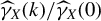
 . Note that the definition of the sample ACFs plotted here is
$\widehat {\gamma } _{X}(k)/\widehat {\gamma }_{X}(0)$
 (cf. the generalized version of ACFs in Abadir, Caggiano, and Talmain, Reference Abadir, Caggiano and Talmain2013).
Figure 1 displays plots of two CI processes and their corresponding ACFs and periodograms for: (i)
$d=0.45$
 (the stationary
$ \{X_{j}\}$
 is a cyclical long-memory process) and (ii)
$d=1$
 (the non-stationary
$\{X_{j}\}$
 is a cyclical unit-root process). The cyclicality in the realization is more pronounced when
$d=1$
 . While the shapes of the ACFs are similar, the range of ACF is wider under the unit root setting (
$d=1$
 ). Notably, the peak of the periodogram at frequency
$ \omega =\pi /16$
 is disproportionately sharper for the cyclical unit root (with
$d=1$
 ) when compared to stationary long-memory process (with
$d=0.45$
 ).
CI
$( \omega ,d)$
 process: plots, ACFs, and periodograms.
Note: CI(
$\omega ,d$
 ) generated by model (5.1) with
$ \omega =\pi /16$
 and
$d=\{0.45, 1\}$
 . Sample size
$n=512$
 .

Figure 1 Long description
The figure consists of two rows of three panels each.
Top Row (d = 0.45):
- Left: Series graph showing a noisy signal fluctuating between -4 and 4 over 512 units.
- Middle: A C F graph showing a damped sinusoidal curve starting at 1.0 and oscillating between 0.5 and -0.5 across 50 lags.
- Right: Periodogram showing a sharp peak reaching a value of 30 at the frequency pi / 16, with negligible activity elsewhere.
Bottom Row (d = 1.00):
- Left: Series graph showing a highly structured oscillating signal with increasing and then decreasing amplitude, ranging from -30 to 40 over 512 units.
- Middle: A C F graph showing a clean, undamped sinusoidal wave oscillating between 1.0 and -1.0 across 50 lags.
- Right: Periodogram showing an extremely high, narrow peak reaching 6500 at the frequency pi / 16.
All periodograms use an x-axis labeled with pi fractions: 0, pi / 16, pi / 4, pi / 2, 3 pi / 4, and pi.
Figure 2 depicts plots, ACFs, and periodograms of a trending CI
$(\omega ,d)$
 process and its de-trended version (5.2) when
$\omega =\pi /16$
 and
$d=0.45$
 . For the trending series, cyclicality inherent in CI is still evident but now the series oscillates around its trend, and the ACF decays slowly in an almost linear fashion.
Trending and de-trended CI
$( \omega ,d)$
 process: plots, ACFs, and periodograms.
Note: Trending and de-trended CI(
$\omega ,d$
 ) process generated by model (5.2) with
$\omega =\pi /16$
 and
$d=0.45$
 . Sample size
$n=512$
 .

Figure 2 Long description
The figure consists of two rows and three columns.
Top Row: Trending Series
* Left: Trending series line graph. The x-axis is units from 0 to 500. The y-axis is values from 0 to 600. The data shows a steady, linear increase with minor fluctuations.
* Middle: A C F (trending series). The x-axis is lags from 0 to 50. The y-axis is correlation from 0.7 to 1. The line shows a very slow, linear decay starting from 1.
* Right: Periodogram (trending series). The x-axis is frequencies from 0 to pi. The y-axis is intensity scaled by 10 super 4. A massive peak occurs at frequency 0, dropping asymptotically to near-zero immediately after.
Bottom Row: De-trended Series
* Left: De-trended series line graph. The x-axis is units from 0 to 500. The y-axis ranges from minus 2 to 6. The data appears as a stationary stochastic process oscillating around a mean of approximately 1.
* Middle: A C F (de-trended series). The x-axis is lags from 0 to 50. The y-axis ranges from minus 1 to 1. The curve shows a damped sinusoidal oscillation, crossing zero at lag 10 and reaching a local maximum near lag 35.
* Right: Periodogram (de-trended series). The x-axis is frequencies from 0 to pi, with a specific label at pi over 16. The y-axis ranges from 0 to 100. There is a sharp, dominant spike at pi over 16, indicating a strong periodic component at that frequency.
Clearly, the cyclical peak in the periodogram at
$\omega =\pi /16$
 is overshadowed by the spike in the periodogram at zero frequency due to the linear trend, a permanent component which has not been removed from the series. Once de-trended, the plot of the data, ACF, and periodogram resemble more those of the original stationary CI series with
$d=0.45$
 .
From Figures 1 and 2, it is evident that the peak in the periodogram of the CI
$(\omega ,d)$
 model becomes more pronounced when
$d$
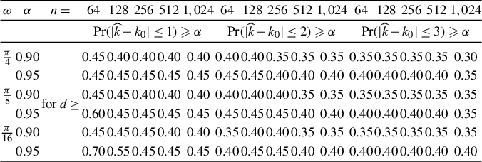
 increases. In Table 2, we assess the probability
$ \Pr \big (\omega \in \lbrack \widehat {\omega }\pm u_{m}]\big )=\Pr \big (| \widehat {k}-k_{0}|\leq m\big )$
 that the unknown
$\omega $
 is within one, two, or three Fourier frequencies of
$\widehat {\omega }$
 . In particular, it reports for a given
$m$
 , the range of memory parameters
$d\geq d_{0,\alpha }$
 for which coverage is larger than
$\alpha =0.9$
 or
$0.95$
 . The lower bound
$ d_{0,\alpha }$
 for
$d$
 , that guarantees
$90\%$
 and
$95\%$
 coverage, seems to be approximately the same across
$\omega $
 for
$n\geq 128$
 , which is in line with the theory. We observe that
$d_{0,\alpha }$
 does not depend on the values
$\omega =\frac {\pi }{4},\frac {\pi }{8},\frac {\pi }{16}$
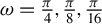 and sample sizes
$n=128,256,512,1,024$
 . For example, for
$\omega =\pi /4$
 and
$ n=125,256,512,1,024,$
 the table indicates that
$\Pr \big (\omega \in \lbrack \widehat {\omega }\pm u_{3}]\big )\geq 0.9$
 for
$d\geq 0.35$
 and
$\Pr \big ( \omega \in \lbrack \widehat {\omega }\pm u_{1}]\big )\geq 0.95$
 for
$d\geq 0.45 $
 . In turn,
$d_{0,\alpha }$
 becomes slightly larger when the sample size is small,
$n=64$
 .
Table 3 reports results for the de-trended CI
$(\omega ,d)$
 model. They are comparable to those in Table 2 as long as sample sizes are not too small (e.g.,
$n\geq 256$
 ).
Shifting the pole at
$\omega =u_{k_{0}}$
 to a non-Fourier frequency
$\omega =u_{k_{0}}+u_{1}/2$
 produces nearly identical results to the baseline scenarios analyzed in Tables 2 and 3 (see Tables 4 and 5 in the Supplementary Material).
Overall, the Monte Carlo study confirms that the estimator
$\widehat {\omega } $
 captures the frequency
$\omega $
 effectively when
$d$
 is relatively large,
$(d\geq 0.4)$
 , and thus when the peak in the spectrum and periodogram is more pronounced. This can be useful in practice, when attempting to identify unknown pronounced cyclical patterns, such as business cycle effects, with confidence.
Minimum value
$d_{0, \alpha }$
 of parameter
$d$
 in CI(
$ \omega ,d$
 ) model such that
$ \omega $
 is contained in
$ \widehat { \omega }\pm u_{m}$
 ,
$m=1,2,3$
 with probability
$ \alpha =0.9,0.95$
 when
$d\geq d_{0, \alpha }$
 .

Table 2 Long description
The table is structured with a hierarchical header. The first column is omega, the second is alpha, and the third is a label for d greater than or equal to. The remaining columns are grouped into three main sections based on probability models:
1. P r (absolute value of omega hat minus omega sub 0 is less than or equal to 1) greater than or equal to alpha.
2. P r (absolute value of omega hat minus omega sub 0 is less than or equal to 2) greater than or equal to alpha.
3. P r (absolute value of omega hat minus omega sub 0 is less than or equal to 3) greater than or equal to alpha.
Each of these three sections contains five sub-columns for n equals 64, 128, 256, 512, and 1,024.
Data rows:
- For omega equals pi over 4:
- alpha 0.90: Values range from 0.45 down to 0.30 as n increases across the three models.
- alpha 0.95: Values range from 0.45 down to 0.35.
- For omega equals pi over 8:
- alpha 0.90: Values range from 0.45 down to 0.35.
- alpha 0.95: Values range from 0.60 down to 0.35.
- For omega equals pi over 16:
- alpha 0.90: Values range from 0.45 down to 0.35.
- alpha 0.95: Values range from 0.70 down to 0.40.
In general, as n increases or the model tolerance (1, 2, or 3) increases, the required minimum value of d decreases.
Note: CI(
$\omega ,d$
 ) in (5.1). Number of replications 2,000.
Minimum value
$d_{0, \alpha }$
 of parameter
$d$
 in de-trended CI(
$ \omega ,d$
 ) model such that
$ \omega $
 is contained in
$\widehat { \omega }\pm u_{m}$
 ,
$m=1,2,3$
 with probability
$ \alpha =0.9,0.95$
 when
$d\geq d_{0, \alpha }$
 .

Table 3 Long description
The table is structured with a multi-level header. The top row lists variables omega, alpha, and n, followed by sample sizes 64, 128, 256, 512, and 1,024 repeated across three main probability conditions. These conditions are defined as:
* P r (absolute value of omega hat minus k sub 0 is less than or equal to 1) greater than or equal to alpha.
* P r (absolute value of omega hat minus k sub 0 is less than or equal to 2) greater than or equal to alpha.
* P r (absolute value of omega hat minus k sub 0 is less than or equal to 3) greater than or equal to alpha.
Data rows are grouped by omega values: pi over 4, pi over 8, and pi over 16. For each omega, alpha values of 0.90 and 0.95 are tested.
Key observations:
* For omega = pi over 4 and alpha = 0.90, d values range from 0.45 at n = 64 down to 0.35 at n = 1,024.
* For omega = pi over 16, several cells for n = 64 are marked with a dash, indicating the confidence interval for omega includes 0.
* Generally, as sample size n increases, the minimum value of parameter d decreases or stabilizes across all probability conditions.
Note: De-trended CI(
$\omega ,d$
 ) in (5.2). “-” indicates that confidence interval for
$\omega $
 includes
$0$
 .
$2,000$
 replications.
6 EMPIRICAL ILLUSTRATION
Many time series display (quasi-)periodic behavior at different frequencies. Examples in economics include macroeconomic time series, such as GDP or IP, which are typically used in the analysis of business cycles (see Harvey and Jaeger, Reference Harvey and Jaeger1993 and Kulish and Pagan, Reference Kulish and Pagan2021, among others). Examples in climate research cover paleoclimatic data, such as global land–ocean temperature (GLOTI), methane (
$\mathrm {CH}_{4}$
 ), and carbon dioxide (
$\mathrm {CO}_{2}$
 ) concentration, ice volume (see McElroy and Politis, Reference McElroy and Politis2024, Proietti and Maddanu, Reference Proietti and Maddanu2024, and references therein). In our empirical illustration, we focus on discerning frequencies at which peaks in the spectrum are evident for: (i) U.S. nominal GDP over the period Q1-1956 to Q4-2019,Footnote
2
(ii) U.S. real IP over the period August 1977 to December 2019,Footnote
3
and (iii)
$\mathrm {CO}_{2}$
 concentration (
$\mathrm {CO}_{2}$
 ) over the period May 1978 to December 2020,Footnote
4
using our estimator introduced in Section 3.
6.1 U.S. Nominal GDP
We start with the analysis of cyclical patterns in quarterly U.S. nominal GDP which is one of the broadest measures of economic activity. A major subfield of macroeconomics focuses on the discovery and extraction of long cycles such as the 2–8 year business cycle, as these convey important information for use when implementing policy adjustments to economic shocks.
Two main considerations in the analysis of business cycles are the choices of (i) seasonal and (ii) “trend” filtering to be applied to the original time series. In (i), adjustment of the raw data from seasonal effects (that are assumed known) typically precedes the analysis of any remaining (unknown) quasi-periodic cycles and is based on linear filtering. One of the most prominent filtering methods is X-12-ARIMA developed by the U.S. Bureau of Census (see Findley et al., Reference Findley, Monsell, Otto and Chen1998). With respect to the “trend” filtering (ii), a number of filters have been considered, such as Hodrick and Prescott (Reference Hodrick and Prescott1997), Baxter and King (Reference Baxter and King1999), Christiano and Fitzgerald (Reference Christiano and Fitzgerald2003), and Beveridge and Nelson (Reference Beveridge and Nelson1981). These filters differ from each other in terms of the assumed type of “trend” present in the original data and dependence assigned to the transformed data. However, as argued in Harvey and Jaeger (Reference Harvey and Jaeger1993), Ghysels, Granger, and Siklos (Reference Ghysels, Granger and Siklos1996), and more recently Kulish and Pagan (Reference Kulish and Pagan2021), use of inappropriate seasonal adjustment and de-trending techniques can lead investigators to report spurious cyclical behavior. More recent contributions allow for the possibility of more flexible fractional differencing where
$d$
 is non-integer and resides in both the stationary and non-stationary domain (see Hart and Jucknewitz, Reference Hart and Jucknewitz2022).
We focus on non-seasonally adjusted U.S. nominal GDP to investigate the existence of persistent long cycles in order to circumvent distorting effects arising from seasonal filtering. Figure 3 (top left panel) depicts the logarithmic transformation
$\log (GDP)$
 of the data where repeated oscillations of different lengths are evident.Footnote
5
In the frequency domain, a large peak of the periodogram at zero frequency dominates over any additional spectral mass at other nonzero frequencies (see Figure 3 [bottom left panel]). Using the ACF domain approach, the properties of this series were analyzed by Abadir et al. (Reference Abadir, Caggiano and Talmain2013) and their tests rejected the ARIMA-type non-cyclical model in favor of the parametric cyclical model considered in their work.
Plots of
$\log $
 transformed, linearly de-trended, and first differenced U.S. non-seasonally adjusted nominal GDP (Q1 1956–Q4 2019), and corresponding periodograms.
Note: Shaded areas are drawn across three frequencies on either side of each peak in the respective periodograms.

Figure 3 Long description
A multi-panel figure with two rows and three columns.
Top Row: Time-series line graphs of U.S. nominal G D P with n equals 256 observations. The x-axis for all three spans Q 1-56 to Q 4-19.
- Top-Left: Log level. The y-axis ranges from 11 to 16. The data shows a consistent, slightly exponential upward trend.
- Top-Middle: Linearly de-trended. The y-axis ranges from 11.2 to 12.0. The data shows a large hump-shaped curve peaking around Q 4-87 before declining.
- Top-Right: First differenced. The y-axis ranges from negative 0.10 to 0.10. The data shows high-frequency oscillations centered around zero.
Bottom Row: Periodograms corresponding to the panels above. The x-axis represents frequencies from 0 to pi.
- Bottom-Left: Periodogram of Log level. The y-axis ranges from 0 to 9000. A massive peak occurs at frequency 0, highlighted by a shaded vertical bar.
- Bottom-Middle: Periodogram minus 3 first frequencies. The y-axis ranges from 0 to 0.07. Significant peaks are highlighted with shaded bars at pi over 43, pi over 16, pi over 2, and pi.
- Bottom-Right: Periodogram of first differenced data. The y-axis ranges from 0 to 0.0140. Three distinct, narrow peaks are highlighted with shaded bars at frequency 0, pi over 2, and pi.
The periodogram of the linearly de-trended
$\log (GDP)$
 series more clearly uncovers the existence of one or more long cycles in the level of nominal GDP, in addition to typical seasonal variations (see Figure 3 [top and bottom middle panels]).Footnote
6
First, clearly-defined peaks are evident at the two seasonal frequencies
$\pi /2$
 and
$\pi $
 (shaded light purple areas),Footnote
7
which coincide with annual and semi-annual cycles, respectively. We also distinguish a mass at the lower frequency of
$\pi /43$
 (shaded light gray area). The length of the corresponding cycle,
$\widehat {\lambda }=2\pi /\widehat {\omega }$
 , equates to 21.3 years, indicative of the longer cycle also found in the analysis of Abadir et al. (Reference Abadir, Caggiano and Talmain2013)—see their Figure 2. Additional mass can be detected at close-by frequencies, such as at frequency
$\pi /16$
 , which translates into a cycle of eight years, the upper bound of the range associated with the business cycle. Overall, without imposing further adjustments to this GDP process, we can infer with confidence that persistent seasonal patterns are evident and well-captured by our estimator, while deciphering distinct longer cycles by means of the periodogram is more ambiguous and requires a more finely-tuned analysis.
Focusing on growth rates in nominal GDP (first-differenced
$\log (GDP)$
 ) instead, produces a periodogram that has significant peaks at the same seasonal frequencies
$\pi /2$
 and
$\pi $
 , but provides a less detailed account of potential cyclical behavior at frequencies close to zero (see Figure 3 [top and bottom right panels]).
6.2 U.S. Real Industrial Production
Turning to the real economy, we also consider the analysis of (quasi-)periodic patterns in U.S. IP which is recorded at a higher frequency (monthly) and focuses on economic activity in the industrial sector (see Ghysels, Reference Ghysels1997; A’Hearn and Woitek, Reference A’Hearn and Woitek2001). As before, we are interested in non-seasonally adjusted U.S. real IP.
Figure 4 (top left panel) plots IP in log levels,
$\log (IP)$
 , where we distinguish regular oscillations of different periods.Footnote
8
This series shows clear signs of significant persistence when looking at the large peak at zero frequency in its corresponding periodogram (bottom left panel of Figure 4). Any signs of additional structure linked to cycles at frequencies away from zero are dominated by the “trend” component, as in the case of nominal GDP.
Plots of
$\log $
 transformed, linearly de-trended, and first differenced U.S. non-seasonally adjusted real industrial production (August 1977–December 2019), and corresponding periodograms.
Note: Shaded areas are drawn across three frequencies on either side of each peak in the respective periodograms.

Figure 4 Long description
A grid of six plots organized into two rows.
Top row contains three time-series line graphs with x-axes spanning August 1977 to December 2019 and n equals 512.
- Top-left: Log level plot showing a long-term upward trend with values rising from 3.8 to 4.6.
- Top-center: Linearly de-trended plot showing cyclical fluctuations between 3.7 and 4.1.
- Top-right: First differenced plot showing high-frequency volatility centered around 0.000.
Bottom row contains three periodograms analyzing frequencies.
- Bottom-left: Periodogram for log level data with a massive peak at frequency 0, y-axis reaching 1800.
- Bottom-center: Periodogram minus 9 first frequencies, showing multiple distinct peaks across the spectrum from pi over 20 to pi. Shaded vertical bars highlight seven specific frequency peaks.
- Bottom-right: Periodogram for first differenced data, showing a similar pattern of seven shaded peaks, with the y-axis scaled to 0.0075.
X-axes for the bottom row are labeled frequencies with markers for pi over 20, pi over 6, pi over 3, pi over 2, 2 pi over 3, 5 pi over 4.5, and pi.
To uncover other peaks in the periodogram, we apply linear de-trending and alternatively first differencing to
$\log (IP)$
 (see Figure 4 [top middle and right panels, respectively]). The corresponding periodograms are depicted in the bottom middle and right panels of Figure 4. In both cases, our estimator identifies substantial mass (peaks) at the seasonal frequencies
$\omega $
 ,
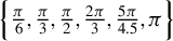
$\Big \{\frac {\pi }{6},\frac {\pi }{3},\frac { \pi }{2},\frac {2\pi }{3},\frac {5\pi }{4.5},\pi \Big \}$
 (shaded light purple areas),Footnote
9
which coincide with cycles of length
$\left \{ 12,6,4,3,2.4,2\right \} $
 months, respectively. Given that seasonal fluctuations are very regular and consistent, it is expected that the peaks at these frequencies are well defined. However, their memory parameters,
$d$
 ’s, are not guaranteed to be uniformly equal to unity (seasonal unit root) which is the typical assumption made in seasonal adjustment methods. Interestingly, we can also distinguish mass at the lower frequency of
$\pi /20$
 (shaded light gray area) which, depending on the focus on level or growth rates of real IP, appears more or less pronounced than those attached to seasonal peaks. The length of the corresponding cycle,
$\widehat {\lambda }=2\pi /\widehat {\omega }$
 , equates to 3.3 years and falls within the 2–8 year bounds assigned to the business cycle. What is evident in both cases is that this mass is not as clearly defined as those at the seasonal frequencies and thus inferring with confidence the existence and persistence of this long cycle requires additional investigation beyond the periodogram.
6.3
$\mathrm {CO}_{2}$
Concentration

Next, we analyze
$\mathrm {CO}_{2}$
 concentration which is instrumental in climate change debates, given its long history. Its monthly series is known to exhibit sawtooth patterns.Footnote
10
The same series was used in the empirical study of Proietti and Maddanu (Reference Proietti and Maddanu2024) which modeled it as a compound of a linear and quadratic trend, an AR(1) process, and six periodic CM-type cycles at predetermined frequencies,
$\omega _{j}=\frac {\pi }{6}j$
 , for
$j=1,2,\ldots ,6$
 .
The log of the series is depicted in the top left panel of Figure 5. The plot encompasses clearly-defined and repeated oscillations over time. A large peak is evident in the periodogram of
$\log (\mathrm {CO}_{2})$
 at zero frequency (bottom left panel of Figure 5). Any signs of peaks at frequencies away from zero are dominated by the mass at
$\omega _{0}=0$
 .
Plots of
$\log $
 transformed, linearly de-trended, and linearly de-trended 12-month moving average
$\mathrm {CO}_{2}$
 concentration (May 1978–December 2020), and corresponding periodograms.
Note: Shaded areas are drawn across three frequencies on either side of each peak in the respective periodograms.

Figure 5 Long description
A multi-panel figure with two rows and three columns. All time series plots in the top row share an x-axis from May 1978 to December 2020 with n equals 512.
Top-left panel, Log level: Y-axis from 5.80 to 6.05. Shows a strong linear upward trend with a tight seasonal oscillation.
Top-center panel, Linearly de-trended: Y-axis from 5.79 to 5.83. The linear trend is removed, revealing a consistent seasonal oscillation that dips slightly in the middle of the time series around August 1999.
Top-right panel, Linearly de-trended 12 M M A: Y-axis from 5.79 to 5.82. A smoothed line showing long-term fluctuations after removing seasonal cycles, with a notable trough around August 1999 and a rise toward 2020.
Bottom-left panel, Periodogram: Y-axis from 0 to 3000, x-axis from 0 to pi frequencies. A single massive vertical spike occurs at frequency 0, representing the dominant trend.
Bottom-center panel, Periodogram minus 3 first freqs: Y-axis from 0 to 0.0025, x-axis marked with pi fractions. Three distinct peaks are highlighted with shaded vertical bars at pi over 64, pi over 6, and pi over 3.
Bottom-right panel, Periodogram minus 3 first freqs with scale 10 super minus 4: Y-axis from 0 to 1. Focuses on the low-frequency power with a shaded peak at pi over 64 and smaller subsequent peaks.
We apply linear de-trending to
$\log (\mathrm {CO}_{2})$
 and compute its corresponding periodogram. These are depicted in the top and bottom middle panels of Figure 5, respectively. There is still evidence of a sizeable peak at zero frequency, so again we disregard the first three Fourier frequencies (
$k=\{0,1,2\}$
 ) and focus our attention on the spectral mass in the remainder of the periodogram. Significant peaks are now revealed at periodic frequencies
$\omega _{1}=\frac {\pi }{6}$
 and
$\omega _{2}=\frac {\pi }{3}$
 (shaded light purple areas), which coincide with stochastic cycles of length 12 and 6 months, respectively. The theoretical results of Sections 2 and 3 indicate that the prominence of these peaks can be translated into memory parameters
$d_{1}$
 and
$d_{2}$
 , in excess of 0.3 when assuming a multi-pole CM model. All potential remaining seasonal cycles must be of limited persistency and thus indistinguishable.Footnote
11
Proietti and Maddanu (Reference Proietti and Maddanu2024) proceed to estimate
$d_{j}$
 ’s corresponding to frequencies
$ \omega _{j}=\frac {\pi }{6}j$
 ,
$j=1,\ldots ,6$
 , over the period January 1958 to June 2020 (
$n=750$
 ), based on a stationary ARCIMA model with
$d<0.5$
 . Using Maximum Likelihood, they find that
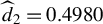
$\widehat {d}_{1}=0.4995$
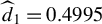 and
$ \widehat {d}_{2}=0.4980$
 when
$\omega _{1}=\frac {\pi }{6}$
 and
$\omega _{2}= \frac {\pi }{3}$
 , respectively, while
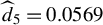
$\widehat {d}_{5}=0.0569$
 when
$\omega _{5}=\frac {5\pi }{6}$
 . In line with our analysis, persistent patterns at frequencies
$\omega _{1}=\frac {\pi }{6}$
 and
$\omega _{2}=\frac {\pi }{3}$
 should be accounted for in the modeling of
$\mathrm {CO}_{2}$
 concentration but not at
$ \omega _{5}=\frac {5\pi }{6}$
 . Proietti and Maddanu (Reference Proietti and Maddanu2024) also conclude that
$ \widehat {d}_{3}$
 ,
$\widehat {d}_{4}$
 , and
$\widehat {d}_{6}$
 corresponding to
$ \omega _{3}=\frac {\pi }{2}$
 ,
$\omega _{4}=\frac {2\pi }{3}$
 , and
$\omega _{6}=\pi $
 hit the upper bound of 0.5. In contrast, our estimator
$ \widehat {\omega }$
 suggests that no important cycles at these frequencies can be identified and hence the need to include cyclical patterns at
$\omega _{3}=\frac {\pi }{2}$
 ,
$\omega _{4}=\frac {2\pi }{3}$
 , and
$\omega _{6}=\pi $
 in the modeling of
$\mathrm {CO}_{2}$
 concentration is debatable.
Separately, from Figure 5 (bottom middle panel), we can distinguish spectral mass at the additional lower frequency,
$\frac {\pi }{64}$
 , which could correspond to the “red noise” component discussed in Proietti and Maddanu (Reference Proietti and Maddanu2024). This translates into a cycle of length of 10.7 years. The additional spectral structure becomes more evident when we model the sawtooth profile of the series: applying a simple (i.e., equal-weight) MA(12) to the de-trended
$\log (\mathrm {CO}_{2})$
 monthly series, we get the top and bottom right panels of Figure 5.
Overall, whether applying an estimation procedure for the memory parameters that permits for
$d>0.5$
 for the cycles identified by our method produces different estimation results to those shown in Proietti and Maddanu (Reference Proietti and Maddanu2024) is an open question. This exercise is beyond the scope of our article and is left for future research.
7 CONCLUSION
In this article, we introduce a class of models which allows for the modeling of persistent cyclical patterns in stationary and non-stationary time series. We show that the cyclicality parameter
$\omega $
 , which is represented by the location of an infinite peak in the spectrum of the time series, can be effectively estimated by maximizing the corresponding periodogram over Fourier frequencies. Theoretical results of this article allow to build confidence intervals for
$\omega $
 . Natural extensions to this work include the development of parameter estimation theory for the ARCIMA model, and formal extension of the modeling to allow for a finite number of infinite peaks in the spectrum.
SUPPLEMENTARY MATERIAL
The supplementary material for this article can be found at https://doi.org/10.1017/S0266466626100504.
FUNDING STATEMENT
This work was supported by the ESRC under Grant RES062230790.
COMPETING INTERESTS
The authors declare that no competing interests exist.








 Open access

