


1 INTRODUCTION
Empirical likelihood (EL) was first introduced by Owen (Reference Owen1988), aiming at tackling the problem of confidence interval (CI) construction for the mean. Later, Owen (Reference Owen1990, Reference Owen1991) extended its applications to confidence region constructions and linear models. Since then, EL methods have been seen in a wide spectrum of statistical applications, such as quantile estimation (Chen and Hall, Reference Chen and Hall1993; Zhou and Jing, Reference Zhou and Jing2003a), estimation for the difference of quantiles (Zhou and Jing, Reference Zhou and Jing2003b; Yang, Yau, and Zhao, Reference Yang, Yau and Zhao2014), mean residual life with biased and censored data (Alemdjrodo and Zhao, Reference Alemdjrodo and Zhao2020), and receiver operating characteristic curve (ROC; Claeskens et al., Reference Claeskens, Jing, Peng and Zhou2003; Qin and Zhou, Reference Qin and Zhou2006; Liu and Zhao, Reference Liu and Zhao2012; Yang and Zhao, Reference Yang and Zhao2012), just to name a few. For a comprehensive review of recent developments in EL, its applications, and its related computational issues, see Chen and Keilegom (Reference Chen and Keilegom2009), Xue and Zhu (Reference Xue and Zhu2012), Nordman and Lahiri (Reference Nordman and Lahiri2014), Lazar (Reference Lazar2021), and Liu and Zhao (Reference Liu and Zhao2023).
Several variants of the traditional EL method have been developed, including Bayesian EL (Lazar, Reference Lazar2003), bias-corrected EL (Zhu and Xue, Reference Zhu and Xue2006), adjusted EL (Chen, Variyath, and Abraham, Reference Chen, Variyath and Abraham2008), and jackknife EL (JEL) (JEL; Jing, Yuan, and Zhou, Reference Jing, Yuan and Zhou2009), among others. In particular, to overcome the computational challenge under nonlinear constraints, Jing et al. (Reference Jing, Yuan and Zhou2009) proposed JEL, a hybrid methodology that adopts jackknife pseudo-values into the construction of the empirical log-likelihood ratio. Under certain regularity conditions, they derived an asymptotic chi-squared distribution for the empirical log-likelihood ratio statistic. Furthermore, they illustrated the performance of JEL in the context of fixed-degree, one-sample or two-sample U-statistics.
Building upon the seminal work of Jing et al. (Reference Jing, Yuan and Zhou2009), we extend the scope of JEL to a novel statistical setting. Specifically, this article investigates JEL in the context of infinite-order U-statistics (Frees, Reference Frees1989). Unlike traditional Wald-type methods, the JEL framework bypasses the need for a plug-in variance estimator, which is particularly beneficial for infinite-order U-statistics where explicit variance estimation can be computationally intensive or analytically infeasible. This allows for a more robust and computationally efficient inference framework in this setting. Additionally, JEL preserves the data-driven shape of confidence regions, which is especially relevant given the potentially non-symmetric asymptotic behavior associated with infinite-order kernels.
Infinite-order U-statistics have numerous applications in marketing (Gómez and Maravall, Reference Gómez and Maravall1998), finance (Nowotarski and Weron, Reference Nowotarski and Weron2015), and econometrics (Bonhomme and Jolivet, Reference Bonhomme and Jolivet2009; Arellano, Blundell, and Bonhomme, Reference Arellano, Blundell and Bonhomme2017). These applications leverage techniques, such as subsampling-based ensemble methods, cross-validation, and subsampling distributions, among others. For example, Bonhomme and Jolivet (Reference Bonhomme and Jolivet2009) used ensemble methods to account for unobserved heterogeneity in credit risk assessment. Nowotarski and Weron (Reference Nowotarski and Weron2015) proposed a quantile regression averaging (QRA) model, which aggregates forecasts from multiple models to construct robust prediction intervals for electricity spot prices. However, the generalization from fixed-degree U-statistics to infinite-order U-statistics is not trivial, as in the latter case, the degree
$k_n$
 of the U-statistic depends on n, and therefore it grows as n goes to infinity. Consequently, existing theoretical results and proofs for fixed-degree U-statistics cannot be extended to the infinite-order setting in a straightforward fashion. DiCiccio and Romano (Reference DiCiccio and Romano2022) stated the sufficient conditions for the validity of a limiting normal distribution of an infinite-order U-statistic. Subsequently, Peng, Coleman, and Mentch (Reference Peng, Coleman and Mentch2022) proved the central limit theorem (CLT) under a so-called generalized U-statistic framework, relaxing one of the core conditions specified in DiCiccio and Romano (Reference DiCiccio and Romano2022). More recently, Mayala et al. (Reference Mayala, Wintenberger, Tillier and Dombry2026) pointed out that a specific Lindeberg condition is needed to establish the limiting normal distribution for subsampling infinite random forests. Additionally, Mayala et al. (Reference Mayala, Scornet, Tillier and Wintenberger2025) also extended the work of Peng et al. (Reference Peng, Coleman and Mentch2022) to handle imbalanced classification tasks.
In this article, we establish the sufficient conditions for the fundamental theory of JEL in the context of infinite-order U-statistics. We confirm that such conditions can be verified explicitly in practice, such as in the case of the maximum test. In addition, our simulation studies suggest that the proposed methodology is robust to the theoretical conditions—it yields satisfactory results in the context of subsampling-based ensemble methods, where the kernel function of the infinite-order U-statistic cannot be expressed in an explicit form. As a further endeavor to alleviate computational cost, we discuss an efficient computational strategy that can be utilized to calculate the jackknife pseudo-values (Efron and Stein, Reference Efron and Stein1981) based on incomplete, infinite-order U-statistics without extra computational effort. Furthermore, we evaluate the performance of the proposed methodology through simulation studies in a number of settings and demonstrate its practical applications using a United States Forest Service (USFS) dataset that predicts the highest bid in dollars at a timber auction. Our main contributions to existing literature are three-fold: first, we develop a general methodology for CI construction of an infinite-order U-statistic that is computationally efficient to realize; second, we push the boundaries of existing U-statistic literature and establish the theoretical framework of JEL for infinite-order U-statistics; and third, we exhibit the applications of our proposed methodology in several interesting scenarios with satisfactory results.
The rest of the article proceeds as follows: we begin in Section 2 by presenting the proposed JEL method for infinite-order U-statistics, including its theoretical foundation and application to incomplete U-statistics. Section 3 then evaluates the method’s effectiveness in constructing CIs for ensemble methods, utilizing subbagging and sub-random forest algorithms (Bühlmann and Yu, Reference Bühlmann and Yu2002; Zaman and Hirose, Reference Zaman and Hirose2009) with linear and multivariate adaptive regression spline (MARS) models. To illustrate the method’s real-world applicability, Section 4 presents a case study predicting the highest bid at a timber auction using a real dataset from the USFS. Section 5 concludes with a summary of our contributions and findings. Additionally, a simulation study on the maximum test, where the main theorem’s conditions are explicitly verified, is included in Appendix C. The detailed technical proofs of the lemmas supporting the main theorem’s derivation are deferred to the Supplementary Material. Additional details on verifying the conditions for the maximum test are also provided there.
2 JACKKNIFE EMPIRICAL LIKELIHOOD FOR INFINITE-ORDER U-STATISTICS
2.1 General Framework
Consider an independent, identically distributed (i.i.d.) sample,
$\mathcal {X}_n=(X_1,\ldots ,X_n)$
 , possibly vector valued, drawn from some underlying distribution F. Suppose the parameter of interest
$\theta _{k_n}$
 can be written as a statistical functional of a kernel function
$\phi _n$
 in the following form:

where
$\phi _n$
 is permutation invariant in its
$k_n$
 components, and its degree
$k_n$
 is dependent on the sample size n. That is,
$k_n\rightarrow \infty $
 as
$n\rightarrow \infty $
 . Different from the classical fixed-degree U-statistics (Hoeffding, Reference Hoeffding1948; Lee, Reference Lee1990), the parameter of interest in this setting depends on
$k_n$
 and n, so we denote it by
$\theta _{k_n}$
 for clarity. Given a target parameter
$\theta _{k_n}$
 and an i.i.d. sample
$\mathcal {X}_n$
 , one can construct an unbiased estimator for
$\theta _{k_n}$
 using a complete, infinite-order U-statistic (Frees, Reference Frees1989), denoted by
$U_n$
 :

where
$(X_{i_1},\ldots ,X_{i_{k_n}})$
 represents a subsample of size
$k_n$
 , and the summation is taken over all possible data subsets of size
$k_n$
 . In the context of growing dimensions,
$\theta _{k_n}$
 does not necessarily converge. However, existing literature has shown the convergence of
$U_n-\theta _{k_n}$
 under certain regularity conditions, see, for instance, Mentch and Hooker (Reference Mentch and Hooker2016), DiCiccio and Romano (Reference DiCiccio and Romano2022), Peng et al. (Reference Peng, Coleman and Mentch2022), and Mayala et al. (Reference Mayala, Scornet, Tillier and Wintenberger2025, Reference Mayala, Wintenberger, Tillier and Dombry2026).
Applications of infinite-order U-statistics span diverse areas, including maximum tests (Lehmann and Romano, Reference Lehmann and Romano2005), Hodges–Lehmann estimators (Hodges and Lehmann, Reference Hodges and Lehmann1963), model comparison techniques via cross-validation (Wang and Lindsay, Reference Wang and Lindsay2014, Reference Wang and Lindsay2017; Wang and Cai, Reference Wang and Cai2021), subsampling distribution (Politis, Romano, and Wolf, Reference Politis, Romano and Wolf1999), and subsampling-based ensemble methods (Bühlmann and Yu, Reference Bühlmann and Yu2002; Mentch and Hooker, Reference Mentch and Hooker2016; Wang and Wei, Reference Wang and Wei2022). In particular, in the context of subsampling-based ensemble methods, one first fits individual base learners based on data subsets of size
$k_n$
 , drawn independently from a learning dataset of size n, then obtains predictions for a fixed test instance
${x}_0$
 using each of the fitted learners, and in the end returns the aggregated prediction. For inferential purposes, it is crucial to evaluate the variability of an infinite-order U-statistic estimator, such as to quantify the uncertainty of predictions obtained from a subsampling-based ensemble estimator.
Some recent work on variance estimation of subsampling-based ensemble methods includes Mentch and Hooker (Reference Mentch and Hooker2016, Reference Mentch and Hooker2017), Wager, Hastie, and Efron (Reference Wager, Hastie and Efron2014), Wager and Athey (Reference Wager and Athey2018), Peng, Mentch, and Stefanski (Reference Peng, Mentch and Stefanski2021), Zhou, Mentch, and Hooker (Reference Zhou, Mentch and Hooker2021), Peng et al. (Reference Peng, Coleman and Mentch2022), and Wang and Wei (Reference Wang and Wei2022). However, due to the dependence of
$k_n$
 on n, most theories and results of the conventional, fixed-degree U-statistics are no longer valid. As a result, it is practically challenging to estimate the variance of an infinite-order U-statistic. Existing methods on this topic do not seem to provide promising numerical results, unless
$k_n$
 is of a much lower order of n. In this article, we aim to bridge this gap by extending the work of Jing et al. (Reference Jing, Yuan and Zhou2009) and employ JEL method to infinite-order U-statistics. The numerical results in Section 3 indicate that our developed methodology yields favorable outcomes across a wide range of applications, exhibiting superior performance compared to competing methods in the existing literature. In addition, its performance is quite robust to the order of
$k_n$
 relative to n. It is worth of attention that the extension of Jing et al.’s work (Jing et al., Reference Jing, Yuan and Zhou2009) is non-trivial, as the theoretical mounting of JEL in this context requires careful probabilistic treatments to handle the dependence of
$k_n$
 on n, which will be discussed and presented in later sections and the Supplementary Material.
Given a complete infinite-order U-statistic as defined in equation (1), denote the jackknife pseudo-values as

where
$U_{n-1}^{(-i)}$
 is a delete-one U-statistic. Specifically, we define
$U_{n-1}^{(-i)}$
 as a U-statistic of degree
$k_n$
 using the same kernel function
$\phi _n$
 , constructed from a delete-one dataset excluding the ith observation (
$i\in \{1,\ldots ,n\})$
 :

It is easy to show that
$(1/n)\sum _{i=1}^n U_{n-1}^{(-i)}=U_n$
 .
As noted by Shi (Reference Shi1984),
$\hat {V}_{n,i}$
 ’s are dependent random variables but asymptotically independent under some mild regularity conditions. Following the notations in Jing et al. (Reference Jing, Yuan and Zhou2009), let
$\mathbf {p}=(p_1,\ldots ,p_n)$
 be a vector of probabilities for jackknife pseudo-values
${\hat {V}_{n,i}}$
 ’s (
$1\leq i\leq n$
 ) such that
$\sum _{i=1}^n p_i=1$
 and
$0\leq p_i\leq 1$
 for
$1\leq i\leq n$
 . It is easy to check that
$U_n=(1/n)\sum _{i=1}^n\hat {V}_{n,i}$
 , and therefore
$E(\hat {V}_{n,i})=\theta _{k_n}$
 and
$\theta _{\mathbf {p}}=\theta _{k_n}$
 . Then, the EL, evaluated at
$\theta _{k_n}$
 , can be written as

And, the JEL ratio, evaluated at
$\theta _{k_n}$
 , is given by

By applying the Lagrange multiplier, under the condition that
$\min _{1\leq i\leq n}{\hat {V}_{n,i}}\leq \theta _{k_n}\leq \max _{1\leq i\leq n}\hat {V}_{n,i}$
 , we have

where
$\lambda $
 satisfies

As a result, the jackknife empirical log-likelihood ratio statistic can be expressed as

A key contribution of this article is the development of a theoretical framework for JEL applied to infinite-order U-statistics. More specifically, under some regularity conditions,
$-2\log R(\theta _{k_n})$
 has a limiting
$\chi ^2_1$
 distribution, which is stated in Theorem 1 and proved in Appendix B. The Supplementary Material presents the proofs for Lemmas 1–6, which establish the theoretical foundation for the proof of Theorem 1.
Before formally stating the main theorem, we introduce some necessary notation.
Let
$h^{(1)}(x_1) = \int \phi _n(x_1,\ldots ,x_{k_n}) dF(x_2) \dots dF(x_{k_n})-\theta _{k_n}$
 and recursively define

where
$\mathcal S_{1,\ldots ,c}^{(j)}$
 is the set that contains all index combinations of size j from
$\{1,\ldots ,c\}$
 . Also, we write

The summation in the second equation is taken over all
$(2k_n-1)!$
 permutations of
$(x_1,\ldots ,x_{2k_n-1})$
 .
We make the following assumptions that are needed in Lemmas 1–6 in the Supplementary Material for the proof of our main result.
A1. The U-statistic
$U_n$
 is non-degenerate with
$E\left [\phi _n^2(X_1,\ldots , X_{k_n})\right ]<\infty $
 .
A2. The degree
$k_n$
 satisfies
$k_n/n^2\rightarrow 0$
 as
$n \to \infty $
 .
A3. Let
$\sigma _c^2=\text {var}\left [h^{(c)}(X_1,\ldots ,X_c)\right ]$
 ,
$1\leq c\leq k_n$
 , and we assume that
$\varsigma _{k_n} = \max _{1 \leq c \leq k_n} \sigma _c = o(n^{1/2}k_n^{-2})$
 .
A4. Under Assumption A1, further assume that
$k_n^3n^{-3/2}\eta _{1,2k_n-1}^{1/2}=o(1)$
 for
$4k_n-3\leq n$
 with a sufficiently large n.
A5. Suppose that there exist a sequence
$\iota _n> 2k_n$
 and a
$\delta \in (0,1)$
 such that

Remark 1. Let
$\phi _n^{(d)}=E\left [\phi _n(X_1,\ldots ,X_{k_n})|X_1,\ldots ,X_d\right ]$
 for
$1\leq d\leq k_n$
 . From Lee (Reference Lee1990) (see equation (9) on page 32), we have

Therefore, a sufficient condition for A3 is to require
$\max _{1\leq d\leq k_n} \text {var}(\phi _n^{(d)}) = o\left (\frac {n}{k_n^4 \cdot 2^{k_n}} \right )$
 , which is satisfied in the example of the maximum test (see Appendix C). Assumption A4 is imposed to bound the remainder term of the jackknife pseudo-values, leveraging its equivalent expression connected to a set of U-statistics of degree
$2k_n-c$
 for
$1\leq c\leq k_n$
 (see Proposition 1 and Lemma 5 in the Supplementary Material for details).
Furthermore, the statement and proof of the main theorem are based on the following two additional conditions:
B1. Without loss of generality, assume that
$E\left [\phi _n(X_1,\ldots ,X_{k_n})\right ]= 0$
 .
B2. Assume
$U_n$
 admits an asymptotic normal distribution, that is,

where
$\zeta _{1,k_n}=\text {cov}(\phi _n(X_1,\ldots ,X_{k_n}),\phi _n(X_1, X_{k_n+1},\ldots ,X_{2k_n-1}))$
 .
Condition B2 is essential for proving the limiting chi-squared distribution in the main theorem (Theorem 1 below). In existing literature (e.g., DiCiccio and Romano, Reference DiCiccio and Romano2022; Peng et al., Reference Peng, Coleman and Mentch2022; Mayala et al., Reference Mayala, Wintenberger, Tillier and Dombry2026), various sets of regularity conditions on the convergence rate of
$k_n$
 have been established. For example, Peng et al. (Reference Peng, Coleman and Mentch2022) stated that, if
$\frac {k_n}{n}\frac {\zeta _{k_n,k_n}}{k_n\zeta _{1,k_n}}\to 0,$
 where
$\zeta _{k_n,k_n}=\text {var}(\phi _n)$
 , the CLT of
$U_n$
 holds. In the most recent work, Mayala et al. (Reference Mayala, Wintenberger, Tillier and Dombry2026) highlighted the necessity of a Lindeberg condition to establish the CLT for subsampling infinite random forests. In Appendix C, we verify that the Lindeberg condition specified in Mayala et al. (Reference Mayala, Wintenberger, Tillier and Dombry2026) holds for the maximum test. Therefore, within the technical framework of Mayala et al. (Reference Mayala, Wintenberger, Tillier and Dombry2026), we can still formally demonstrate the validity of condition B2 for the maximum test.
Theorem 1. Let
$X_1, X_2, \ldots $
 be i.i.d. random variables, possibly vector valued, that are drawn from a common distribution function F. Assume Assumptions A1–A5 and Conditions B1 and B2. In addition, assume that

If, furthermore,
$\zeta _{1,k_n}$
 is bounded from below by a positive constant, then

Following Theorem 1, to construct a
$100(1-\alpha )\%$
 asymptotic CI for
$\theta _{k_n}$
 , one needs to solve the following two equations simultaneously:


where
$\chi ^2_{1}(1-\alpha )$
 denotes the
$100(1-\alpha )$
 th percentile of
$\chi ^2_{1}$
 . It can be shown that the JEL ratio statistic, that is,
$-2\log R(\theta _{k_n})$
 given in equation (4), is monotonously decreasing for
$\theta _{k_n}\in (\min \{\hat {V}_{i}\}, \overline {\hat {V}})=(\min \{\hat {V}_{i}\}, U_{n})$
 and monotonously increasing for
$\theta _{k_n}\in (\overline {\hat {V} }, \max \{{\hat {V}_{n,i}}\})= (U_{n}, \max \{{\hat {V}_{n,i}}\})$
 , where
$\overline {\hat {V}}=(1/n)\sum _{i=1}^n\hat {V}_{n,i}=U_n$
 (see Lemma 4 in the Supplementary Material for the proof). Hence, one can apply the bi-section method (Wu, Reference Wu2005) using these ranges as initial search intervals to identify the two roots of equations (5) and (6) simultaneously.
Remark 2. A milder condition on
$\phi _n$
 (Assumption A5) is to only require that there exists a sequence
$\iota _n> 2k_n$
 with
${\lim _{n \to \infty } n^{-(\iota _n/2-k_n)} E\left (|\phi _n(X_1,\ldots ,X_{k_n})|^{\iota _n}\right ) = 0}$
 . More discussion on this can be found in Lemma 6 in the Supplementary Material. The condition on
$\zeta _{1,k_n}$
 in the main theorem is essential for bounding the remainder term of the JEL log-likelihood ratio statistic
$-2\log R(\theta _{k_n})$
 . Although we acknowledge that this condition can be challenging to verify in certain complex practical settings, our numerical results consistently demonstrate that the developed inferential framework is remarkably robust to deviations from this constraint. In addition, all conditions for Theorem 1 are explicitly verifiable. We demonstrate their applicability in Appendix C, where we show that these requirements are strictly satisfied in the case of the maximum test statistic.
Remark 3. In the recent work of Chiang, Matsushita, and Otsu (Reference Chiang, Matsushita and Otsu2025), the authors also extended the JEL framework to infinite-order U-statistics with applications to honest random forests, including a valuable discussion on the “sparse-subsampling” scenario and a modified JEL procedure under sparse-subsampling. However, our study offers several distinct contributions. First, we introduce a partition-sampling scheme that enhances the computational efficiency of jackknife pseudo-values. Second, Chiang et al. (Reference Chiang, Matsushita and Otsu2025) focused on honest random forests and discusses sparse-subsampling asymptotics, while our work provides a broader scope of applications to infinite-order U-statistics, including examples on bagging and the maximum test. Finally, we provide explicit verification of the regularity conditions for the maximum test and demonstrate the practical utility of our method through a real-world application using USFS timber auction data (see Section 4), while Chiang et al. (Reference Chiang, Matsushita and Otsu2025) is based on simulation studies within honest random forests.
2.2 Application to Incomplete, Infinite-Order U-Statistics
Since
$U_n$
 ’s degree
$k_n$
 may grow with n, computing
$U_n$
 can be quite expensive or even infeasible in practice. As a result, one often considers its incomplete counterpart in real-life applications. For example, in the case of subsampling-based ensemble methods, such as subbagging and sub-random forest (Bühlmann, Reference Bühlmann2003; Zaman and Hirose, Reference Zaman and Hirose2009), one often fits a simple regression or classification tree (Breiman et al., Reference Breiman, Friedman, Stone and Olshen1984) on B independently drawn subsamples, where B may be much smaller than
$\binom {n}{k_n}$
 . This results in an incomplete, infinite-order U-statistic. We denote it by

where
$\phi _n$
 represents the tree fitting algorithm in the given context, and
$\mathcal {X}_{S_1},\ldots ,\mathcal {X}_{S_B}$
 are data subsets of size
$k_n$
 , where
$\mathcal {X}_{S_b}=\{X_i: i\in S_b,\ S_b\subset \{1,\ldots ,n\},\ \text {and }|S_b|=k_n\}$
 , drawn independently from a given learning dataset
$\mathcal {X}_n$
 .
$U_{n,B}$
 serves as a Monte Carlo approximation of the complete, infinite-order U-statistic
$U_n$
 . The theoretical foundations of our developed method, such as the asymptotic normal distribution of
$U_n$
 , remain valid for
$U_{n,B}$
 provided that
$B/n\rightarrow \infty $
 . A formal statement of the main theorem in the case of incomplete, infinite-order U-statistics can be found in Corollary 1 below. We also discuss these asymptotic requirements in the context of the numerical studies presented later in the article. In what follows, we discuss the application of JEL to incomplete, infinite-order U-statistics through a computationally efficient partition-sampling scheme (Wang and Lindsay, Reference Wang and Lindsay2014).
Suppose we want to aggregate predictions over B individual learners fitted on random subsamples (e.g., decision trees). Without loss of generality, assume that n is divisible by
$k_n$
 . The partition-sampling strategy proceeds as follows: we start with randomly partitioning the learning dataset of size n into
$n/k_n$
 blocks of data subsets, each of size
$k_n$
 , and then repeat the random partitioning for
$B/(n/k_n)=Bk_n/n$
 times to obtain a total number of B subsamples. For each block, we fit a simple tree algorithm and make predictions at a fixed test instance, denoted as
${x}_0$
 . In the end, we average over the B predictions to obtain
$U_{n,B}$
 , that is, an incomplete, infinite-order U-statistic.
To calculate the delete-one U-statistics based on the generated B subsamples, we first recognize that for a fixed index
$i\ (1\leq i\leq n)$
 , there is one and only one block of data subset per partition that contains observation i. Therefore, building on the same set of partitioned subsamples, we can realize each of its delete-1 variants as an average over
$(n/k_n-1)\times (Bk_n/n)=B-Bk_n/n$
 subsamples. In particular, we do not need to refit these individual trees. Therefore, calculating n additional delete-1 U-statistics, that is,
$U_{n-1,B}^{(-i)}$
 ’s, essentially does not incur any additional computational cost. (Note that although we reserve the same subscript B when denoting the constructed delete-1 incomplete U-statistics, each of them is calculated using less than B subsamples.) We show in our later simulation studies that this strategy makes the proposed methodology quite computationally efficient to realize.
Following the aforementioned definitions of
$U_{n,B}$
 and
$U_{n,B}^{(-i)}$
 , we define the jackknife pseudo-values based on incomplete U-statistics in an analogous form as below:

Without loss of generality, we assume that the kernel functions for
$U_{n,B}$
 and
$U_{n-1,B}^{(-i)}$
 are identical. This is a reasonable assumption in practice: for example, if
$k_n$
 is a fraction of n, rounding
$k_n$
 to its ceiling will always result in the same value for
$k_n$
 and
$k_{n-1}$
 , which leads to the same kernel function for both
$\phi _n$
 and
$\phi _{n-1}$
 . Then, the following results hold.
Proposition 1. If the kernel functions for
$U_{n,B}$
 and
$U_{n-1,B}$
 are identical, we have

The proof for Proposition 1 can be found in Appendix A.
Corollary 1. Assume the same assumptions and conditions as in Theorem 1. If the subsample size B satisfies
$B/n\rightarrow \infty $
 , the log-likelihood ratio statistic computed through incomplete U-statistics still admits the following limiting chi-squared distribution:

where
$\log R_B(\theta _{k_n})=-\sum _{i=1}^n\log \left [1+\lambda (\hat {V}_{B,i}-\theta _{k_n})\right ]$
 .
Theorem 3.1 in DiCiccio and Romano (Reference DiCiccio and Romano2022) states that the asymptotic normal distribution still holds for
$U_{n,B}$
 , provided that
$B/n\rightarrow \infty $
 . Based on this result, the limiting chi-squared distribution stated in Theorem 1 can be generalized to incomplete, infinite-order U-statistics. Note that conditions for B may be formulated differently in specific contexts, such as subsampling infinite random forests (Mayala et al., Reference Mayala, Wintenberger, Tillier and Dombry2026) and honest random forests (Chiang et al., Reference Chiang, Matsushita and Otsu2025). The statement in Corollary 1 is essentially analogous to Theorem 1 in Chiang et al. (Reference Chiang, Matsushita and Otsu2025). Consequently, one can construct a CI for
$\theta _{k_n}$
 based on incomplete, infinite-order U-statistics, following the same procedure as described in Section 2.1.
Remark 4. We acknowledge that the modified JEL method in Chiang et al. (Reference Chiang, Matsushita and Otsu2025) yields an improved finite-sample performance in the context of honest random forests when the number of subsamples B is not sufficiently large (i.e., their so-called “sparse-subsampling” scenario), as demonstrated in their simulation study. However, as our simulations reveal, if B is sufficiently large, the standard JEL-based CI eventually approaches the target coverage probability.
3 SIMULATION STUDIES
In this section, we evaluate the performance of the proposed method to construct asymptotic CIs of an infinite-order U-statistic in three different settings: (1) subsampling-based ensemble methods with data generated from a simple linear regression (SLR) model, (2) subsampling-based ensemble methods with data generated from a MARS model, and (3) the maximum test. We present the first two simulations in Section 3 and defer the last example to Appendix C. For the maximum test, one can express the kernel function of its associated infinite-order U-statistic in a closed form, and therefore it is possible to verify the conditions of Theorem 1 explicitly. More elaborations on this can be found in Appendix C.
3.1 Simple Linear Regression Model
In the first simulation study, we consider an SLR model, given by

where
$X_1, \dots , X_n$
 are i.i.d.
$\text {Uniform}([0,2])$
 random variables, and
$\epsilon _1, \dots , \epsilon _n$
 are i.i.d.
$N(0,1)$
 . We set the learning sample size n to be
$500$
 and the subsample size
$k_n$
 to be either
$0.05n$
 ,
$0.10n$
 ,
$0.20n$
 , or
$0.50n$
 . In addition, we used
$B = 100, 1,000, 5,000, \text { or } 10,000$
 random subsamples of size
$k_n$
 to build each ensemble estimator, namely,
$U_{n,B}$
 . Individual trees in each ensemble were realized using the R function randomForest by setting ntree
$=1$
 . This function is part of the randomForest package (Liaw and Wiener, Reference Liaw and Wiener2002) in R (R Core Team, 2024) that employs Breiman’s random forest algorithm. Since there is only one feature, sub-random forest is identical to subbagging in this case.
For each simulated dataset, we implemented the proposed JEL method to construct 95% CIs for
$\theta _{k_n}(x_0)=E[U_{n,B}(x_0)]=E(\phi _n)$
 at test instance
$x_0=1$
 , where
$\phi _n$
 represents the tree-fitting algorithm realized based on a training sample of size
$k_n$
 . Because in practice computing the complete infinite-order U-statistic
$U_n$
 is unfeasible, we approximated the true parameter value
$\theta _{k_n}(x_0)$
 by the empirical mean of
$U_{n,B}$
 with
$B=10^4$
 out of 500 randomly generated datasets. Table 1 summarizes the approximate true parameter values, the average lower bound (LB) and upper bound (UB), standard deviations of LB and UB, and the average width of the proposed CIs realized by JEL. All results were based on
$R=500$
 independently simulated datasets, and we adopted the bi-section algorithm in Wu (Reference Wu2005) to identify each CI.
Simulation results of the proposed method under the SLR model

Table 1 Long description
The table is split into two horizontal blocks.
Top Block: Compares Number of trees = 100 and Number of trees = 1,000.
- The first column is k sub n with values 0.05 n, 0.10 n, 0.20 n, and 0.50 n.
- The second column is theta sub k sub n (x sub 0) with values ranging from 1.995 to 1.984.
- For 100 trees, as k sub n increases, the Interval Width grows significantly from 1.880 to 7.735.
- For 1,000 trees, the Interval Width is narrower, growing from 0.737 to 2.928 as k sub n increases.
- S D (Standard Deviation) values for Lower Bound (L B) and Upper Bound (U B) are provided for both tree counts.
Bottom Block: Compares Number of trees = 5,000 and Number of trees = 10 super 4.
- The k sub n and theta values remain the same as the top block.
- For 5,000 trees, the Interval Width ranges from 0.533 (at k sub n = 0.05 n) to 2.056 (at k sub n = 0.50 n).
- For 10 super 4 trees, the Interval Width is the most precise, ranging from 0.502 to 1.917.
- Across all sections, increasing the number of trees reduces the interval width and standard deviation, while increasing k sub n increases the interval width.
To compare our method with existing approaches, we also constructed 95% CIs using an asymptotic normal distribution:

where the standard deviation
$\text {SD}(U_{n,B})$
 was estimated by one of the following four methods: the unbiased variance estimator (denoted by “Unbiased”) and its negative-corrected variant (denoted by “Unbiased
$+$
 ”) (Wang and Wei, Reference Wang and Wei2022), the infinitesimal jackknife (IJ; Jaeckel, Reference Jaeckel1972; Zhou et al., Reference Zhou, Mentch and Hooker2021), and the internal variance estimation method (IV; Mentch and Hooker, Reference Mentch and Hooker2016). These four methods were also studied in Wang and Wei (Reference Wang and Wei2022), where the unbiased variance estimator and its variant were originally proposed. Specifically, the Unbiased
$+$
 estimator replaces any negative variance estimates by a positive-definite variance estimate, as recommended in Wang and Wei (Reference Wang and Wei2022). The IV method is essentially a double-layer Monte-Carlo method. Therefore, to ensure comparability, we set the total number of iterations (i.e., the inner-loop iterations multiplied by the outer-loop iterations) equal to the specified value of B in the simulation.
The results based on the proposed JEL method are summarized in Table 1. In addition, we evaluated the coverage probability of different methods, calculated as the proportion of the 500 independent simulations where the constructed CI contains the true parameter value
$\theta _{k_n}(x_0)$
 . These results are summarized in Table 2. Moreover, we record the average computational time (in seconds) for each method across the 500 simulations in Table 3. The simulations were performed on a single personal computing machine without parallel programming.
Comparison of coverage probabilities of different methods under the SLR model

Table 2 Long description
The table is structured with columns for k sub n, Number of trees (100, 1,000, 5,000, 10,000), Proposal, and Competing methods (Unbiased, Unbiased plus, I J, and I V).
* For k sub n = 0.05 n:
- 100 trees: Proposal 1.000, Unbiased 0.862, Unbiased plus 0.870, I J 1.000, I V 1.000.
- 1,000 trees: Proposal 0.996, Unbiased 0.950, Unbiased plus 0.952, I J 0.992, I V 0.994.
- 5,000 trees: Proposal 0.968, Unbiased 0.952, Unbiased plus 0.952, I J 0.966, I V 0.980.
- 10,000 trees: Proposal 0.962, Unbiased 0.970, Unbiased plus 0.970, I J 0.958, I V 0.978.
* For k sub n = 0.10 n:
- 100 trees: Proposal 1.000, Unbiased 0.896, Unbiased plus 0.900, I J 1.000, I V 1.000.
- 1,000 trees: Proposal 0.998, Unbiased 0.970, Unbiased plus 0.970, I J 0.996, I V 1.000.
- 5,000 trees: Proposal 0.964, Unbiased 0.970, Unbiased plus 0.970, I J 0.940, I V 0.986.
- 10,000 trees: Proposal 0.950, Unbiased 0.974, Unbiased plus 0.974, I J 0.932, I V 0.996.
* For k sub n = 0.20 n:
- 100 trees: Proposal 1.000, Unbiased 0.976, Unbiased plus 0.976, I J 1.000, I V 1.000.
- 1,000 trees: Proposal 1.000, Unbiased 0.990, Unbiased plus 0.990, I J 0.994, I V 0.998.
- 5,000 trees: Proposal 0.966, Unbiased 0.990, Unbiased plus 0.990, I J 0.910, I V 0.998.
- 10,000 trees: Proposal 0.940, Unbiased 0.992, Unbiased plus 0.992, I J 0.896, I V 1.000.
* For k sub n = 0.50 n:
- 100 trees: Proposal 1.000, Unbiased 1.000, Unbiased plus 1.000, I J 0.984, I V 1.000.
- 1,000 trees: Proposal 0.996, Unbiased 1.000, Unbiased plus 1.000, I J 0.614, I V 1.000.
- 5,000 trees: Proposal 0.948, Unbiased 1.000, Unbiased plus 1.000, I J 0.438, I V 1.000.
- 10,000 trees: Proposal 0.920, Unbiased 1.000, Unbiased plus 1.000, I J 0.422, I V 1.000.
Comparison of average computational time (in seconds) across different methods under the SLR model

Table 3 Long description
The table is organized into columns: n equals 500, Number of trees, Proposal, and Competing methods which include Unbiased, Unbiased plus, I J, and I V. Data is grouped by four values of k sub n.
* For k sub n equals 0.05 n:
- 100 trees: Proposal 0.6, Unbiased 0.5, Unbiased plus 0.6, I J 2.7, I V 0.2.
- 1,000 trees: Proposal 5.5, Unbiased 5.2, Unbiased plus 5.8, I J 21.8, I V 1.9.
- 5,000 trees: Proposal 30.7, Unbiased 29.2, Unbiased plus 29.2, I J 89.6, I V 12.2.
- 10,000 trees: Proposal 63.2, Unbiased 58.5, Unbiased plus 58.5, I J 182.4, I V 23.2.
* For k sub n equals 0.10 n:
- 100 trees: Proposal 0.6, Unbiased 0.6, Unbiased plus 0.7, I J 3.0, I V 0.2.
- 1,000 trees: Proposal 6.1, Unbiased 5.5, Unbiased plus 5.5, I J 23.5, I V 1.9.
- 5,000 trees: Proposal 36.7, Unbiased 29.8, Unbiased plus 29.8, I J 100.8, I V 12.7.
- 10,000 trees: Proposal 72.8, Unbiased 59.5, Unbiased plus 59.5, I J 207.6, I V 23.7.
* For k sub n equals 0.20 n:
- 100 trees: Proposal 0.7, Unbiased 0.6, Unbiased plus 0.6, I J 3.2, I V 0.2.
- 1,000 trees: Proposal 6.6, Unbiased 5.8, Unbiased plus 5.8, I J 24.3, I V 2.0.
- 5,000 trees: Proposal 39.6, Unbiased 31.5, Unbiased plus 31.5, I J 104.2, I V 13.3.
- 10,000 trees: Proposal 76.9, Unbiased 63.2, Unbiased plus 63.2, I J 216.5, I V 24.7.
* For k sub n equals 0.50 n:
- 100 trees: Proposal 0.9, Unbiased 0.8, Unbiased plus 0.8, I J 3.4, I V 0.3.
- 1,000 trees: Proposal 8.5, Unbiased 7.9, Unbiased plus 7.9, I J 27.7, I V 3.1.
- 5,000 trees: Proposal 50.1, Unbiased 40.2, Unbiased plus 40.2, I J 122.0, I V 15.1.
- 10,000 trees: Proposal 97.5, Unbiased 85.1, Unbiased plus 85.1, I J 268.8, I V 28.0.
Tables 1 and 2 reveal that the proposed method performs well for constructing CIs of the ensemble method in the SLR setting. For a given subsample size
$k_n$
 , as the number of trees B increases, the overall performance of the proposed method improves, that is, it attains a narrower CI and smaller standard deviations for both the LB and UB. In addition, the coverage probability approaches the nominal level of 0.95 with a greater B. When
$k_n$
 is relatively large, for example,
$k_n=0.2n$
 or above, one needs to increase the number of trees in order to ensure a reliable CI. The standard deviations of the UB and LB decrease significantly when B increases from 100 to 1,000. However, increasing B further does not appear to lead to significant additional reduction in the standard deviations of the LB and UB. In general, using
$B=5,000$
 trees for each ensemble seems to provide satisfactory results for the coverage probability across different subsample sizes under the SLR model.
Compared to the other competing methods shown in Table 2, our proposed method achieves coverage probabilities closer to the target 95% level in all cases except one occasion, particularly as the number of trees or the degree of the U-statistic increases. Notably, the performance of competing methods deteriorates significantly with a larger U-statistic degree, primarily due to violation of the assumption on
$k_n$
 for the asymptotic normal distribution of
$U_n$
 . Furthermore, the coverage probabilities of the unbiased estimation method and its variant tend to increase with the number of trees, but they do not appear to approach the true level as B becomes larger. It is also worth mentioning that the unbiased variance estimator can produce negative variance estimates, as noted in (Wang and Lindsay (Reference Wang and Lindsay2014) and Wang and Wei (Reference Wang and Wei2022). In particular, the chance of getting a negative variance estimate can be as high as 8.4%, as shown in Table 2 of Wang and Wei (Reference Wang and Wei2022). In comparison, the IJ method corresponds to coverage probabilities that are significantly below the target level when B or
$k_n$
 increase. The IV method, on the other hand, has a large positive bias for estimating the true variance of the U-statistic, resulting in overly liberal CIs, especially when
$k_n$
 is not small.
As detailed in Table 3, computational cost is primarily driven by the ensemble size (i.e., the number of trees per ensemble) and less affected by the U-statistic degree
$k_n$
 . Our proposed method exhibits computational efficiency comparable to Unbiased and Unbiased
$+$
 , while the IV method appears to be slightly less expensive to realize. Conversely, the cost of the IJ method scales with the learning sample size, rendering it 3–4 times as expensive in this setting. These computational trends were consistent across both the SLR model and the MARS model. Therefore, we omit the results for computational comparison in the subsequent section.
3.2 MARS Model
In the second simulation study, we consider the MARS model, also known as Friedman #1, which was proposed by Friedman (Reference Friedman1991) and also studied in Bühlmann (Reference Bühlmann2003), Mentch and Hooker (Reference Mentch and Hooker2016), and Wang and Wei (Reference Wang and Wei2022):

where
$\textbf {X}_1 ,\ldots , \textbf {X}_n\text { are i.i.d. }\text {Uniform}([0,1]^{5})$
 , and
$\epsilon _1, \ldots ,\epsilon _n\text { are i.i.d. }N(0,1)$
 . The regression function is given by
$f(\mathbf {x}) = 10 \sin (\pi x_1x_2) + 20(x_3 - 0.05)^2 + 10x_4 + 5x_5$
 .
We set the learning sample size to
$n=500$
 or
$2,000$
 and the subsample size
$k_n=0.05n$
 ,
$0.10n$
 ,
$0.20n$
 , and
$0.50n$
 . To assess the effect of ensemble size, we varied the number of trees (B) from
$100$
 to
$10^5$
 . Given each simulated dataset, we calculated the proposed 95% CIs for the expected prediction at the test point
$\mathbf {x}_{0}$
 where all five features were set to
$0.5$
 . Individual trees were built using the randomForest function with ntree
$=1$
 in R. For subbagging, all five features were used for splitting at each internal node, while sub-random forests used
$\lfloor 5/3\rfloor =1$
 random feature for each binary splitting, as suggested by Breiman (Reference Breiman2001).
To establish a baseline for evaluating CIs, we approximated the true value of the parameter
$\theta _{k_n}(\mathbf {x}_0)$
 by the empirical mean of
$U_{n, B}$
 with
$B=10^4$
 trees over 500 random datasets. All these approximate true parameter values are reported in Tables 4–7.
Simulation results of the proposed method for subbagging under the MARS model (
$n=500$
 )

Table 4 Long description
The image consists of five data tables showing simulation results for subbagging under the M A R S model. Each table corresponds to a different Number of trees: 100, 1,000, 5,000, 10 super 4, and 10 super 5.
All tables share the same column structure:
* k sub n: Subsample size (0.05n, 0.10n, 0.20n, 0.50n).
* theta k sub n (x sub 0): Estimated value.
* Mean: Lower Bound (L B) and Upper Bound (U B).
* Interval: Width.
* S D: Standard Deviation Lower Bound (L B) and Upper Bound (U B).
* Coverage: Probability value.
* Time: Computational time.
Key trends across the panels:
* As the Number of trees increases from 100 to 10 super 5, the Interval Width significantly decreases for all k sub n values. For example, at k sub n = 0.05n, the width drops from 10.197 (100 trees) to 1.656 (10 super 5 trees).
* Computational Time increases substantially with the number of trees, rising from 0.7 at 100 trees to 1,303.2 at 10 super 5 trees for the 0.05n subsample.
* Coverage values remain high, starting at 1.000 for lower tree counts and slightly adjusting toward 0.950 to 0.962 as the tree count reaches 10 super 5.
* The theta k sub n (x sub 0) values remain consistent across all tree counts for each respective k sub n level (e.g., 17.535 for 0.05n).
Simulation results of the proposed method for subbagging under the MARS model (
$n=2,000$
 )

Table 5 Long description
The data is presented in five panels corresponding to the Number of trees: 100, 1,000, 5,000, 10 super 4, and 10 super 5. Each table uses rows defined by k sub n values (0.05n, 0.10n, 0.20n, and 0.50n) and columns for theta sub k sub n (x sub 0), Mean (L B and U B), Interval Width, S D (L B and U B), Coverage, and Time.
* For 100 trees: As k sub n increases from 0.05n to 0.50n, Interval Width increases from 17.713 to 67.002, and Time increases from 2.4 to 6.3. Coverage remains constant at 1.000.
* For 1,000 trees: Interval Width ranges from 5.743 to 21.403. Time increases from 25.4 to 71.9. Coverage remains 1.000.
* For 5,000 trees: Interval Width ranges from 2.790 to 10.002. Time increases from 129.1 to 343.7. Coverage remains 1.000.
* For 10 super 4 trees: Interval Width ranges from 2.152 to 7.412. Time increases from 249.2 to 615.8. Coverage remains 1.000.
* For 10 super 5 trees: Interval Width ranges from 1.343 to 3.853. Time increases significantly from 4,296.2 to 8,195.3. Coverage slightly decreases, ranging from 0.964 to 0.984.
Across all panels, as the Number of trees increases, the Interval Width for the same k sub n value decreases significantly while the computation Time increases.
Simulation results of the proposed method for sub-random forest under the MARS model (
$n=500$
 )

Table 6 Long description
The image contains five tables representing simulation results for tree counts of 100, 1,000, 5,000, 10 super 4, and 10 super 5. Each table shares a common header structure with columns for k sub n, theta sub k sub n (x sub 0), Mean (Lower Bound L B and Upper Bound U B), Interval Width, S D (L B and U B), Coverage, and Time.
* For 100 trees: As k sub n increases from 0.05n to 0.50n, the Interval Width increases from 11.389 to 43.137, and Time increases from 0.7 to 1.0.
* For 1,000 trees: For the same k sub n range, Interval Width increases from 3.856 to 14.111, and Time increases from 0.7 to 10.7.
* For 5,000 trees: Interval Width increases from 2.180 to 6.863, and Time increases from 33.6 to 50.4.
* For 10 super 4 trees: Interval Width increases from 1.868 to 5.321, and Time increases from 68.2 to 93.2.
* For 10 super 5 trees: Interval Width increases from 1.531 to 3.400, and Time increases from 1,246.4 to 1,571.8.
Across all tables, theta sub k sub n (x sub 0) remains relatively stable around 18.3. Coverage remains high, typically between 0.974 and 1.000. As the number of trees increases, the Interval Width significantly decreases while the computation Time increases.
Simulation results of the proposed method for sub-random forest under the MARS model (
$n=2,000$
 )

Table 7 Long description
The data is presented in five sub-tables categorized by the number of trees. Each table includes columns for k sub n, theta sub k sub n (x sub 0), Mean (L B and U B), Interval Width, S D (L B and U B), Coverage, and Time.
* Number of trees = 100: For k sub n = 0.05n, theta is 18.265, Interval Width is 21.279, and Time is 2.4. For k sub n = 0.50n, theta is 18.639, Interval Width is 76.623, and Time is 6.1.
* Number of trees = 1,000: For k sub n = 0.05n, theta is 18.265, Interval Width is 6.813, and Time is 26.1. For k sub n = 0.50n, theta is 18.639, Interval Width is 25.433, and Time is 72.0.
* Number of trees = 5,000: For k sub n = 0.05n, theta is 18.265, Interval Width is 3.198, and Time is 134.3. For k sub n = 0.50n, theta is 18.639, Interval Width is 11.545, and Time is 351.7.
* Number of trees = 10 super 4: For k sub n = 0.05n, theta is 18.265, Interval Width is 1.757, and Time is 267.3. For k sub n = 0.50n, theta is 18.639, Interval Width is 8.316, and Time is 644.3.
* Number of trees = 10 super 5: For k sub n = 0.05n, theta is 18.265, Interval Width is 1.271, and Time is 3,267.4. For k sub n = 0.50n, theta is 18.639, Interval Width is 3.444, and Time is 9,650.1.
Across all tables, as the number of trees increases, the Interval Width decreases significantly while the computation Time increases. Coverage remains consistently near 1.000.
The complexity of the MARS data-generation process significantly increases the difficulty in evaluating the variability of the ensemble estimator, a phenomenon also observed by Wang and Wei (Reference Wang and Wei2022). Consistent with our earlier observations in Section 3.1, the overall performance of the proposed method improves as the number of trees B increases, given a fixed subsample size
$k_n$
 . In Tables 4 and 6, when the learning sample size is
$n=500$
 , with
$B=10^5$
 trees, the coverage probability of the constructed CI is fairly close to the nominal level of 0.95 in both the subbagging and sub-random forest scenarios. In comparison, results in Tables 5 and 7 reveal that when the learning sample size is
$n=2,000$
 , the coverage probability of the constructed CI all remains at 100% at
$B=100$
 to
$10^4$
 . However, as the number of trees B increases further, the coverage probability improves. In particular, when
$B=10^5$
 , the coverage probability is around 97%–98% for most of the settings under the MARS model. Although not included in the simulation results in this article, we did notice in our numerical investigations that this figure further approaches
$95\%$
 when B is increased to
$10^6$
 . It seems that for a more complex model, one needs to set B to be large enough to ensure satisfactory performance of the CI construction. This conclusion can be explained by the theoretical foundation of the developed methodology, that is, the asymptotic chi-squared distribution of
$-2\log R(\theta _{k_n})$
 relies on the asymptotic normality of the infinite-order U-statistic. And, as DiCiccio and Romano (Reference DiCiccio and Romano2022) noted, the limiting normal distribution holds for an incomplete, infinite-order U-statistic under the condition that
$n/B\rightarrow 0$
 . In other words, as the sample size n grows, one needs to increase B to better satisfy the condition for the asymptotic normality of an incomplete, infinite-order U-statistic.
We further evaluated the coverage probabilities of our proposed method against the four previously discussed competitors under the MARS model using subbagging and sub-random forests estimators when
$n=500$
 (see Tables 8 and 9). Consistent with the SLR results, our method outperforms all competing methods except in a few instances. In particular, the unbiased method and its variant suffer from overcoverage at larger degrees
$k_n$
 . Furthermore, in this setting, the chance that the unbiased variance estimator yields negative values is as high as 20%, as reported in Wang and Wei (Reference Wang and Wei2022). In addition, the IV method performs poorly by producing a coverage probability that is at or close to 100% even with a relatively small degree
$k_n$
 . Conversely, the coverage probability of the IJ method declines sharply as B increases, eventually falling way below the target 95% level. Similar conclusions can be made for
$n=2,000$
 . From a different aspect, conclusions on their computational costs as discussed in Section 3.1 still hold in the MARS model: IJ is significantly more expensive to calculate than the other methods; its computational cost also increases with a larger sample size or a higher-dimensional dataset.
Comparison of coverage probabilities of different methods under the MARS model, using the subbagging estimator

Table 8 Long description
The table is organized into four main sections based on the value of k sub n.
Section 1: k sub n = 0.05 n
- 100 trees: Proposal 1.000, Unbiased 0.788, Unbiased plus 0.820, I J 1.000, I V 1.000.
- 1,000 trees: Proposal 1.000, Unbiased 0.862, Unbiased plus 0.906, I J 0.998, I V 0.998.
- 5,000 trees: Proposal 0.998, Unbiased 0.954, Unbiased plus 0.958, I J 0.994, I V 0.998.
- 10 super 4 trees: Proposal 0.978, Unbiased 0.988, Unbiased plus 0.988, I J 0.970, I V 0.998.
- 10 super 5 trees: Proposal 0.962, Unbiased 1.000, Unbiased plus 1.000, I J 0.946, I V 0.976.
Section 2: k sub n = 0.10 n
- 100 trees: Proposal 1.000, Unbiased 0.808, Unbiased plus 0.852, I J 1.000, I V 1.000.
- 1,000 trees: Proposal 1.000, Unbiased 0.978, Unbiased plus 0.978, I J 0.998, I V 1.000.
- 5,000 trees: Proposal 0.992, Unbiased 0.994, Unbiased plus 0.994, I J 0.988, I V 1.000.
- 10 super 4 trees: Proposal 0.984, Unbiased 0.998, Unbiased plus 0.998, I J 0.970, I V 1.000.
- 10 super 5 trees: Proposal 0.960, Unbiased 1.000, Unbiased plus 1.000, I J 0.932, I V 0.988.
Section 3: k sub n = 0.20 n
- 100 trees: Proposal 1.000, Unbiased 0.956, Unbiased plus 0.958, I J 1.000, I V 1.000.
- 1,000 trees: Proposal 1.000, Unbiased 1.000, Unbiased plus 1.000, I J 1.000, I V 1.000.
- 5,000 trees: Proposal 0.994, Unbiased 1.000, Unbiased plus 1.000, I J 0.984, I V 1.000.
- 10 super 4 trees: Proposal 0.986, Unbiased 1.000, Unbiased plus 1.000, I J 0.964, I V 1.000.
- 10 super 5 trees: Proposal 0.954, Unbiased 1.000, Unbiased plus 1.000, I J 0.900, I V 0.996.
Section 4: k sub n = 0.50 n
- 100 trees: Proposal 1.000, Unbiased 1.000, Unbiased plus 1.000, I J 1.000, I V 1.000.
- 1,000 trees: Proposal 1.000, Unbiased 1.000, Unbiased plus 1.000, I J 0.998, I V 1.000.
- 5,000 trees: Proposal 0.998, Unbiased 1.000, Unbiased plus 1.000, I J 0.910, I V 1.000.
- 10 super 4 trees: Proposal 0.992, Unbiased 1.000, Unbiased plus 1.000, I J 0.830, I V 1.000.
- 10 super 5 trees: Proposal 0.950, Unbiased 1.000, Unbiased plus 1.000, I J 0.608, I V 1.000.
Comparison of coverage probabilities of different methods under the MARS model, using the sub-random forest estimator

Table 9 Long description
The table is organized into seven columns: k sub n, Number of trees, Proposal, and Competing methods which is subdivided into Unbiased, Unbiased plus, I J, and I V. Data is grouped by four values of k sub n.
* For k sub n = 0.05 n:
- 100 trees: Proposal 1.000, Unbiased 0.764, Unbiased plus 0.818, I J 1.000, I V 1.000.
- 1,000 trees: Proposal 1.000, Unbiased 0.820, Unbiased plus 0.880, I J 1.000, I V 1.000.
- 5,000 trees: Proposal 0.992, Unbiased 0.956, Unbiased plus 0.966, I J 1.000, I V 1.000.
- 10 super 4 trees: Proposal 0.988, Unbiased 0.984, Unbiased plus 0.984, I J 0.984, I V 1.000.
- 10 super 5 trees: Proposal 0.972, Unbiased 1.000, Unbiased plus 1.000, I J 0.972, I V 0.986.
* For k sub n = 0.10 n:
- 100 trees: Proposal 1.000, Unbiased 0.788, Unbiased plus 0.822, I J 1.000, I V 1.000.
- 1,000 trees: Proposal 1.000, Unbiased 0.970, Unbiased plus 0.980, I J 1.000, I V 1.000.
- 5,000 trees: Proposal 0.996, Unbiased 0.998, Unbiased plus 0.998, I J 0.998, I V 1.000.
- 10 super 4 trees: Proposal 0.992, Unbiased 1.000, Unbiased plus 1.000, I J 0.986, I V 1.000.
- 10 super 5 trees: Proposal 0.974, Unbiased 1.000, Unbiased plus 1.000, I J 0.952, I V 0.994.
* For k sub n = 0.20 n:
- 100 trees: Proposal 1.000, Unbiased 0.960, Unbiased plus 0.968, I J 1.000, I V 1.000.
- 1,000 trees: Proposal 1.000, Unbiased 1.000, Unbiased plus 1.000, I J 1.000, I V 1.000.
- 5,000 trees: Proposal 0.998, Unbiased 1.000, Unbiased plus 1.000, I J 1.000, I V 1.000.
- 10 super 4 trees: Proposal 0.992, Unbiased 1.000, Unbiased plus 1.000, I J 0.986, I V 1.000.
- 10 super 5 trees: Proposal 0.974, Unbiased 1.000, Unbiased plus 1.000, I J 0.904, I V 0.994.
* For k sub n = 0.50 n:
- 100 trees: Proposal 1.000, Unbiased 1.000, Unbiased plus 1.000, I J 1.000, I V 1.000.
- 1,000 trees: Proposal 1.000, Unbiased 1.000, Unbiased plus 1.000, I J 1.000, I V 1.000.
- 5,000 trees: Proposal 1.000, Unbiased 1.000, Unbiased plus 1.000, I J 0.982, I V 1.000.
- 10 super 4 trees: Proposal 0.996, Unbiased 1.000, Unbiased plus 1.000, I J 0.920, I V 1.000.
- 10 super 5 trees: Proposal 0.974, Unbiased 1.000, Unbiased plus 1.000, I J 0.723, I V 1.000.
Remark 5. In real-life applications, the ensemble size, B, can be chosen by monitoring the stability of the CI’s bounds. Our simulations reveal that the JEL-based CI becomes stable for a sufficiently large B. Hence, to balance accuracy with computational cost, we recommend selecting the smallest B where further increases no longer significantly change the CI. Furthermore, we note that a more complex underlying data-generating process may require a higher value of B to ensure stability.
4 REAL DATA EXAMPLE
In this section, we present a real data example to demonstrate the practical applications of the proposed methodology. We consider a dataset on USFS timber auctions, where publicly owned forests were sold to private sector organizations through auctions. Previous research that concerns timeber auctions include Baldwin, Marshall, and Richard (Reference Baldwin, Marshall and Richard1997), Haile (Reference Haile2001), and Haile and Tamer (Reference Haile and Tamer2003). For this particular illustration, we focus on sealed-bid auctions in Forest Service Regions 1 and 5 between 1982 and 1990. The same dataset was also analyzed in Liu and Luo (Reference Liu and Luo2007).
We used the same trimmed dataset as in Liu and Luo (Reference Liu and Luo2007), where salvage sales and sales for small businesses were excluded. Additionally, we also discarded observations that have only one bidder for the given auction. The final trimmed dataset has 1,714 observations. For ease of implementation of the partition-sampling scheme, we randomly sampled 1,710 auctions as our learning dataset and selected one of the remaining observations as the test sample (denoted by
$\mathbf {x}_0$
 ).
The primary response of interest is the log-transformed highest bid in dollars (Y). To account for various auction-specific characteristics, we included predictors such as the log-transformed size of the tract in acres (
$X_1:=$
 log_acres), log-transformed estimated timber volume in MBF (
$X_2:=$
 log_vol_sum), log-transformed per-MBF values for appraisal (
$X_3:=$
 AppValue_avg), log-transformed estimated selling price (
$X4:=$
 log_SellValue_avg), estimated harvesting costs (
$X_5:=$
 log_cost_avg), log-transformed estimated manufacturing costs (
$X_6:=$
 log_MtgCost_avg), the Herfindahl–Hirschman Index (
$X_7:=$
 HHI), and the Forest Service region (
$X_8:=$
 D5 which is a binary indicator with level 1 representing Region 5 and 0 representing Region 1). We utilized subbagging and sub-random forest estimators to predict the log-transformed highest bid in dollars of the test instance. In this context, the subbagging estimator can be written in the form of an incomplete, infinite-order U-statistics as follows:

where
$\phi _n$
 represents the regression tree algorithm where all eight predictors are considered at each binary splitting, and
$\mathcal {X}_{S_b}$
 is a random subsample of size
$k_n$
 taken from the given learning dataset. Similarly, the sub-random forests estimator can be written as

where
$\phi _n^\ast $
 denotes the tree fitting algorithm where only a random subset of three features, out of eight, is considered at each internal splitting.
We considered four choices of the subsample size, namely,
$k_n=0.05n, 0.10n, 0.20n$
 , and
$0.50n$
 . In addition, we chose three different values of B: 100, 1,000, and 5,000. Our numerical explorations showed that an ensemble size of
$B=5,000$
 is sufficient for the given dataset. Therefore, we did not explore larger values for B. For each choice of
$k_n$
 and B, we calculated the U-statistic, that is,
$U_{n,B}^{\text {bag}}$
 or
$U_{n,B}^{\text {rf}}$
 , which is an unbiased estimator for the expected value of log bid for the test instance, that is,
$\theta _{k_n}(\mathbf {x}_0)$
 . Then, we constructed the proposed 95% JEL-based CI. All results are summarized in Table 10. The results reveal that the width of the constructed 95% CI decreases as the number of trees increases; this is consistent with our observations in the simulation studies in Section 3. In particular, the change in interval width is dramatic when B increases from 100 to 1,000, which is even more visible when fitting a sub-random forests estimator.
Constructed 95% confidence interval for the test instance at different values of
$k_n$
 and B, using either the subbagging or the sub-random forests estimators

Table 10 Long description
The table is divided into two vertical sections.
Top Section: Subbagging Estimator.
Columns include Subbagging (k sub n values), No. of trees (B), F sub n, B super bag, 95% C I, and Interval width.
- For k sub n = 0.05n: At 100 trees, C I is (8.623, 11.713) with width 3.090. At 5,000 trees, C I narrows to (9.962, 10.436) with width 0.474.
- For k sub n = 0.10n: At 100 trees, C I is (8.311, 12.305) with width 3.994. At 5,000 trees, C I is (10.011, 10.585) with width 0.574.
- For k sub n = 0.20n: At 100 trees, C I is (8.159, 12.623) with width 4.464. At 5,000 trees, C I is (10.043, 10.706) with width 0.663.
- For k sub n = 0.50n: At 100 trees, C I is (7.579, 13.258) with width 5.679. At 5,000 trees, C I is (9.911, 10.963) with width 1.052.
Bottom Section: Sub-R F (Sub-random forests) Estimator.
Columns include Sub-R F (k sub n values), No. of trees (B), F sub n, B super r f, 95% C I, and Interval width.
- For k sub n = 0.05n: At 100 trees, C I is (8.211, 11.939) with width 3.728. At 5,000 trees, C I is (9.726, 10.245) with width 0.519.
- For k sub n = 0.10n: At 100 trees, C I is (7.556, 12.486) with width 4.930. At 5,000 trees, C I is (9.702, 10.424) with width 0.722.
- For k sub n = 0.20n: At 100 trees, C I is (6.705, 13.543) with width 6.838. At 5,000 trees, C I is (9.598, 10.636) with width 1.038.
- For k sub n = 0.50n: At 100 trees, C I is (3.648, 16.681) with width 13.033. At 5,000 trees, C I is (9.329, 11.111) with width 1.782.
Across both estimators, increasing the number of trees from 100 to 5,000 significantly reduces the interval width.
5 SUMMARY
This article introduces a general framework for applying JEL to infinite-order U-statistics. The central contribution is proving that the jackknife empirical log-likelihood ratio statistic, built upon infinite-order U-statistics, asymptotically follows a chi-squared distribution under specific regularity conditions. The article validates these conditions for the maximum test and proposes an efficient computational method for constructing jackknife pseudo-values using incomplete, infinite-order U-statistics. We present simulation studies in the context of subsampling-based ensemble and the maximum test to construct CIs for ensemble methods. The simulation results suggest that the proposed methodology exhibits prominent performance across different simulation settings. In addition, it shows robust performance even when the asymptotic conditions cannot be explicitly verified, or when the degree of the U-statistic
$k_n$
 grows at a faster rate than what is required in the main theorem. In addition, we further showcase our method by a real data example, using a USFS timber auction dataset.
A PROOF OF PROPOSITION 1
Proof of Proposition 1
To show
$(1/n)\sum _{i=1}^n U_{n-1,B}^{(-i)}=U_{n,B}$
 , we need to first note that

where
$\phi _n$
 denotes the kernel function for both
$U_{n,B}$
 and
$U_{n-1,B}$
 .
Each block of data subset contains
$k_n$
 observations. And, for the delete-i calculation of
$U_{n-1,B}^{(-i)}$
 ,
$Bk_n/n$
 blocks of such data subsets are removed. Therefore, when summing over i where
$X_i\notin \mathcal {S}_b$
 , each data subset is counted repeatedly for
$n-k_n$
 times. That is,

where
$\mathcal {S}_1,\ldots ,\mathcal {S}_B$
 are the B data subsets obtained through the previous partition sampling procedure. Hence,

Furthermore, since
$(1/n)\sum _{i=1}^n U_{n-1,B}^{(-i)}=U_{n,B}$
 , it is easy to see that

B PROOF OF THEOREM 1
Building upon Lemmas 1–6 in the Supplementary Material, we detail the proof of Theorem 1 below.
Corollary B.1. Let
$W_n=\max _{1\leq i\leq n}|{\hat {V}_{n,i}}-\theta _{k_n}|$
 . If
$E\{\phi _n^2(X_1,\ldots , X_{k_n})\}<\infty $
 , then with probability one,
$W_n=o_p(k_nn^{1/2})$
 and
$n^{-1}\sum _{i=1}^n|{\hat {V}_{n,i}}-\theta _{k_n}|^3=o_p(k_n^3n^{1/2}\zeta _{1,kn}+k_nn^{1/2})$
 .
Proof. First, we can re-express
$U_n$
 as follows:

for any fixed
$i\in \{1,\ldots ,n\}$
 . As a result,

Thus,
$|{\hat {V}_{n,i}}-\theta _{k_n}|\leq (2k_n-1)\max |\phi _n(X_1,\ldots ,X_{k_n})|+|\theta _{k_n}|=(2k_n-1)H_n+|\theta _{k_n}|$
 . From Lemma 6,
$W_n=o_p(k_n n^{1/2})$
 . Together with the result in Lemma 5, we have

Proof of the Main Theorem
In the following, we complete the proof of the main theorem.
Proof. From Lemma 4, with probability tending to one, the true parameter
$\theta _{k_n}$
 satisfies
$\min _{1\leq i\leq n}{\hat {V}_{n,i}}<\theta _{k_n}<\max _{1\leq i\leq n} {\hat {V}_{n,i}}$
 . Thus, the solution to equations (B.1) and (B.2) exists and is unique:


In what follows, we first show the root of equation (B.1). From equation (B.1), we have

By condition B2 and the fact that
$(1/n)\sum _{i=1}^n{\hat {V}_{n,i}}=U_n$
 , the second term is
$O_p(\sqrt {k_n^2\zeta _{1,k_n}/n})$
 . From Lemma 5,
$S_n=k_n^2\zeta _{1,k_n}+o(k_n^2\zeta _{1,k_n})+o_p(1)$
 . It follows that
$|\lambda _n|/(1+|\lambda _n|W_n)=O_p(k_n^{-1}n^{-1/2}\zeta _{1,k_n}^{-1/2})$
 . Hence, by Corollary B.1,

Under the assumption that
$\zeta _{1,k_n}\geq c_0$
 for some positive real constant
$c_0$
 , we have

Let
$\gamma _i=\lambda _n({\hat {V}_{n,i}}-\theta _{k_n})$
 . From Corollary B.1 and equation (B.3),

When expanding equation (B.1), we have

where the last term is bounded from above by

Under the assumption that
$\zeta _{1,k_n}\geq c_0>0$
 and
$k_n=o(n^{1/2})$
 , the last line above becomes
$o_p(1)$
 .
Therefore, we may write

where
$|\beta |=o_p(k_n^{-2}\zeta _{1,k_n}^{-1})$
 . By equation (B.4), we may expand
$\log (1+\gamma _i)=\gamma _i-\gamma _i^2/2+\eta _i$
 , where, for some finite
$B>0$
 , we have
$P(|\eta _i|\leq B|\gamma _i|^3; 1\leq i\leq n)\rightarrow 1$
 as
$n\rightarrow +\infty $
 .
Recall that, in the main text, we define

where
$\lambda $
 satisfies equation (B.1), that is,
$f(\lambda ):=\frac {1}{n}\sum _{i=1}^n({\hat {V}_{n,i}}-\theta _{k_n})/\{1+\lambda ({\hat {V}_{n,i}}-\theta _{k_n})\}=0$
 .
By plugging equations (B.5) and (B.6) into
$-2\log R(\theta _{k_n})$
 , where
$\log R(\theta _{k_n})=\sum _{i=1}^n\log \left \lbrace 1+\lambda ({\hat {V}_{n,i}}-\theta _{k_n})\right \rbrace $
 , we have

For the first term, we have
$n(U_n-\theta _{k_n})^2/S_n\xrightarrow {D}\chi _1^2$
 by condition B2 and Lemma 5. For the second term, it follows from Lemma 5 and equation (B.5) that

Under the assumption that
$\zeta _{1,k_n}\geq c_0$
 and
$k_n=o(n^{1/2})$
 , we have
$|-nS_n\beta ^2|=o_p(1)$
 .
For the last term, by Corollary B.1 and equation (B.5), we have that with probability one,

In the end, by combining all the above results, it follows that
$-2\log R(\theta _{k_n})\xrightarrow {D}\chi _1^2$
 .
C SIMULATION STUDY ON THE MAXIMUM TEST
We present an example on the maximum test that is also considered in DiCiccio and Romano (Reference DiCiccio and Romano2022) (see their Examples 2.1 and 4.1). Different from the applications to subbagging and sub-random forest as discussed in Section 3 of the article, in this example, the associated kernel function of the infinite-order U-statistic (i.e., the maximum test statistic) can be expressed in a closed form. As a result, we can verify the conditions of Theorem 1 explicitly.
Assume
$X_1,\ldots , X_n$
 are independent normal random variables with mean
$\mu _i$
 and variance 1. Suppose one is interested in testing whether
$H_0: \mu _1=\cdots =\mu _n=0$
 against
$H_a:$
 some of the
$\mu _i$
 ’s are nonzero. As noted in DiCiccio and Romano (Reference DiCiccio and Romano2022), if the index set i’s for
$\mu _i\ne 0$
 is sparse, a better approach than the uniformly most powerful invariant (UMPI) level-
$\alpha $
 test is to perform a maximum test. The maximum test has found its applications in the econometrics of structural breaks (Andrews, Reference Andrews1993), the detection of financial bubbles (Phillips, Wu, and Yu, Reference Phillips, Wu and Yu2011), and the detection of high-dimensional signal (Cai, Liu, and Xia, Reference Cai, Liu and Xia2014). In these applications, the maximum test is preferred due to the sparsity of signals.
For ease of discussion, the problem can be formulated as follows: for some
$\epsilon>0$
 (
$\epsilon $
 can be either fixed or dependent on n. In the latter case,
$\epsilon =\epsilon _n\to 0$
 as
$n\to \infty $
 .) and
$k=k_n$
 , we want to identify the maximum level-
$\alpha $
 test such that at least
$k_n$
 of the
$\mu _i$
 ’s satisfy
$\mu _i>\epsilon $
 . Then, the associated test statistic can be written as an infinite-order U-statistic with a kernel function given by

for some small
$\epsilon>0$
 . One rejects the null hypothesis if the U-statistic takes a large value. Under the null hypothesis,
$\theta _{k_n}=E(U_n)=\exp (\epsilon ^2k_n/2)$
 . In addition, it can be derived that

For any fixed
$\epsilon> 0$
 , if
$(\log n)^{-1} k_n \to 0$
 as
$n \to \infty $
 , then
$\zeta _{1,k_n}$
 is bounded away from zero for all large n, and

The latter result recovers the limiting normal distribution of
$U_n$
 based on the central limit theorem derived in Peng et al. (Reference Peng, Coleman and Mentch2022). The detailed proof for this scenario can be found in Lemma 7 in the Supplementary Material. On the other hand, if
$\epsilon _n\to 0$
 as
$n\to 0$
 , Lemma 8 in the Supplementary Material states the conditions to ensure that
$\zeta _{1,k_n}$
 is bounded away from zero and a limiting normal distribution of
$U_n$
 can be established in the given context. In this case, because
$\zeta _{1,k_n}$
 is bounded below by a positive constant, the Lindeberg condition (see equation (H1) in Mayala et al., Reference Mayala, Wintenberger, Tillier and Dombry2026), namely,
$n\zeta _{1,k_n}\rightarrow \infty $
 as
$n\to \infty $
 , holds. Therefore, under the theoretical framework of Mayala et al. (Reference Mayala, Wintenberger, Tillier and Dombry2026), the asymptotic normality of
$U_n$
 is still valid.
Furthermore, it can be confirmed that all the other conditions in Theorem 1 are met. For example, the technical conditions for Lemma 6 in the Supplementary Material can be verified as presented below. First, we can show that

and thus

If we choose
$\iota _n \leq \kappa \log n$
 for some
$\kappa> 0$
 , then it can be shown that

and thus the choice of
$\iota _n = {2(k_n+1) \over \delta - \kappa k_n \epsilon ^2}$
 leads to condition (4) in Lemma 7 in the Supplementary Material. To guarantee the existence and compatibility of such a choice of
$\iota _n$
 , it suffices to require that

Since
$k_n \epsilon ^2 = O(1)$
 , there exists a
$c_2> 0$
 such that
$k_n\epsilon ^2 \leq c_2$
 for all large n, and, as a result,

holds for all large n. Therefore, it suffices to require that

Let
$\kappa = \delta /(2c_2),$
 which minimizes the restriction on
$k_n$
 , then equation (4) in the Supplementary Material holds if

Since
$\delta \in (0,1)$
 can be chosen arbitrarily close to one, it suffices to require that

Hence, the conditions for Lemma 7 in the Supplementary Material hold, and so does Theorem 1, provided that
$k_n$
 is of a desired order of n. Further details on verifying the conditions of Theorem 1 can be found in Section 2 of the Supplementary Material. In addition, the simulation results in Section 3 also suggest that the performance of the developed methodology is quite robust, even if the condition on
$k_n$
 ’s growth rate is not strictly satisfied.
We generated
$R=500$
 independent samples of size
$n=100$
 under
$H_0$
 , that is,
$X_1,\ldots ,X_n$
 are i.i.d.
$N(0,1)$
 . For each of the simulated dataset, we approximated the complete infinite-order U-statistic with B random subsets of size
$k_n$
 , where B was taken to be either
$100, 1,000$
 , or
$2,000$
 , and
$k_n=0.05n, 0.10n, 0.20n$
 , or
$0.50n$
 . We set
$\epsilon =0.01$
 or
$0.1$
 for illustration. Then, we constructed 95% CIs for
$\theta _{k_n}$
 , under the jackknife empirical likelihood framework, based on each dataset. Tables C1 and C2 summarize the simulated mean and standard deviation of the CIs, as well as the coverage probability out of 500 iterations. In addition, we also reported the computational time in seconds for constructing a single CI on average.
Simulation results on maximum test statistic (
$\epsilon =0.01$
 )

Table C1 Long description
The table is divided into three vertical sections based on the number of trees: 100, 1,000, and 2,000. Each section contains columns for k sub n, theta sub k sub n, Mean (L B and U B), Interval Width, S D (L B and U B), Coverage, and Time in seconds.
* Section 1: Number of trees = 100. For k sub n values of 0.05n, 0.10n, 0.20n, and 0.50n, the theta sub k sub n remains near 1.000. Interval width increases from 0.027 to 0.331 as k sub n increases. Coverage ranges from 0.990 to 0.998. Processing time increases from 5.284 to 7.474 seconds.
* Section 2: Number of trees = 1,000. For the same k sub n values, theta sub k sub n remains near 1.000. Interval width increases from 0.021 to 0.214. Coverage is stable around 0.960 to 0.966. Processing time is significantly higher, ranging from 50.418 to 54.983 seconds.
* Section 3: Number of trees = 2,000. Theta sub k sub n remains near 1.000. Interval width increases from 0.020 to 0.205. Coverage remains stable between 0.954 and 0.962. Processing time is the highest, ranging from 94.175 to 113.298 seconds.
Simulation results on maximum test statistic (
$\epsilon =0.1$
 )

Table C2 Long description
The table is divided into three panels based on the number of trees. Each panel contains columns for k sub n, theta sub k sub n, Mean (L B and U B), Interval Width, S D (L B and U B), Coverage, and Time in seconds.
Panel 1: Number of trees = 100.
* For k sub n = 0.05 n: theta = 1.025, Mean L B = 0.892, U B = 1.167, Width = 0.275, S D L B = 0.045, U B = 0.063, Coverage = 0.992, Time = 5.253.
* For k sub n = 0.10 n: theta = 1.051, Mean L B = 0.765, U B = 1.355, Width = 0.590, S D L B = 0.079, U B = 0.146, Coverage = 0.994, Time = 5.428.
* For k sub n = 0.20 n: theta = 1.105, Mean L B = 0.472, U B = 1.769, Width = 1.297, S D L B = 0.126, U B = 0.368, Coverage = 0.984, Time = 5.708.
* For k sub n = 0.50 n: theta = 1.284, Mean L B = minus 0.826, U B = 3.401, Width = 4.227, S D L B = 0.577, U B = 1.770, Coverage = 0.958, Time = 6.969.
Panel 2: Number of trees = 1,000.
* For k sub n = 0.05 n: theta = 1.025, Mean L B = 0.924, U B = 1.133, Width = 0.209, S D L B = 0.045, U B = 0.057, Coverage = 0.956, Time = 47.468.
* For k sub n = 0.10 n: theta = 1.051, Mean L B = 0.841, U B = 1.273, Width = 0.432, S D L B = 0.083, U B = 0.127, Coverage = 0.960, Time = 51.003.
* For k sub n = 0.20 n: theta = 1.105, Mean L B = 0.655, U B = 1.574, Width = 0.919, S D L B = 0.133, U B = 0.315, Coverage = 0.954, Time = 57.053.
* For k sub n = 0.50 n: theta = 1.284, Mean L B = minus 0.085, U B = 2.664, Width = 2.749, S D L B = 0.161, U B = 1.372, Coverage = 0.886, Time = 71.064.
Panel 3: Number of trees = 2,000.
* For k sub n = 0.05 n: theta = 1.025, Mean L B = 0.926, U B = 1.131, Width = 0.205, S D L B = 0.045, U B = 0.057, Coverage = 0.960, Time = 88.829.
* For k sub n = 0.10 n: theta = 1.051, Mean L B = 0.845, U B = 1.268, Width = 0.423, S D L B = 0.083, U B = 0.127, Coverage = 0.956, Time = 108.075.
* For k sub n = 0.20 n: theta = 1.105, Mean L B = 0.667, U B = 1.562, Width = 0.895, S D L B = 0.134, U B = 0.312, Coverage = 0.956, Time = 110.372.
* For k sub n = 0.50 n: theta = 1.284, Mean L B = minus 0.030, U B = 2.609, Width = 2.639, S D L B = 0.130, U B = 1.338, Coverage = 0.882, Time = 135.783.
When the theoretical conditions are satisfied, the results demonstrate that the coverage probability of the JEL-based CI approaches the nominal level 0.95 as B increases. In addition, the performance of the proposed method is pretty robust to the deviation from the constraint on
$k_n$
 . For instance, when
$k_n$
 increases to
$0.2n$
 , a level that does not fully satisfy the required order of
$k_n$
 in Theorem 1, the coverage probability of the JEL-based CI is still fairly close to 0.95 when
$B=1,000\text { or }2,000$
 . Only when
$\epsilon =0.1$
 and
$k_n=0.5n$
 , the coverage probability of the CI is noticeably below the target level.
SUPPLEMENTARY MATERIAL
The supplementary material for this article can be found at https://doi.org/10.1017/S0266466626100681.
FUNDING STATEMENT
The work of Y.Z. is partially supported by the Simons Foundation (MPS-TSM-00638679).
COMPETING INTEREST STATEMENT
The authors declare that no competing interests exist.


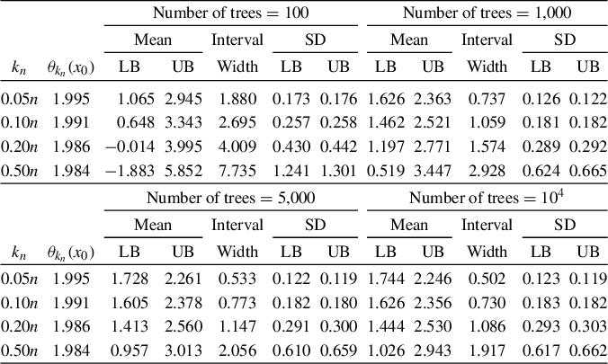
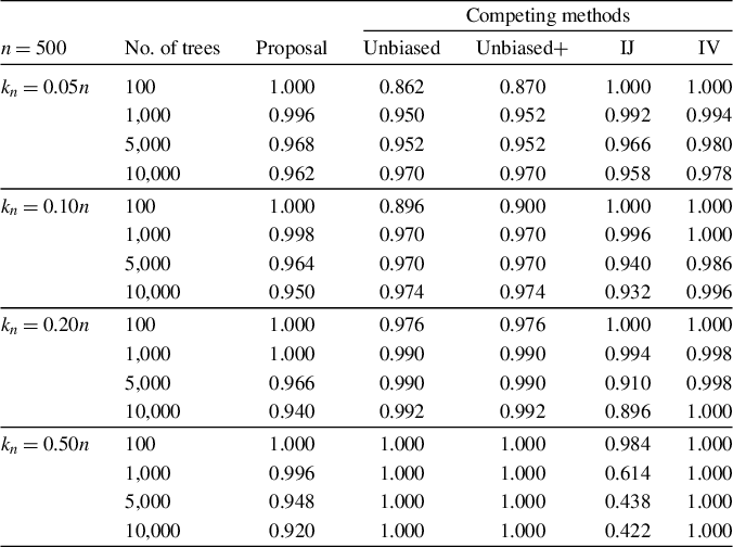
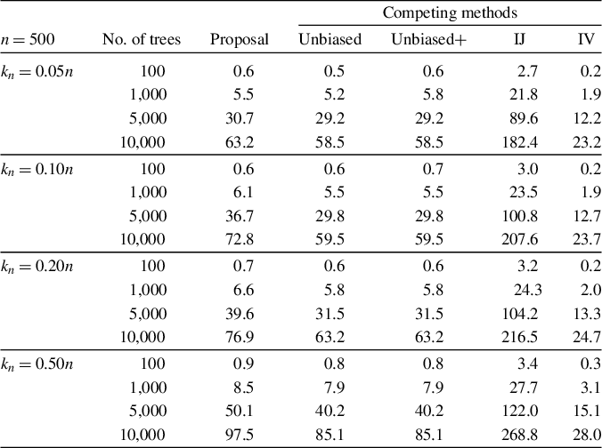
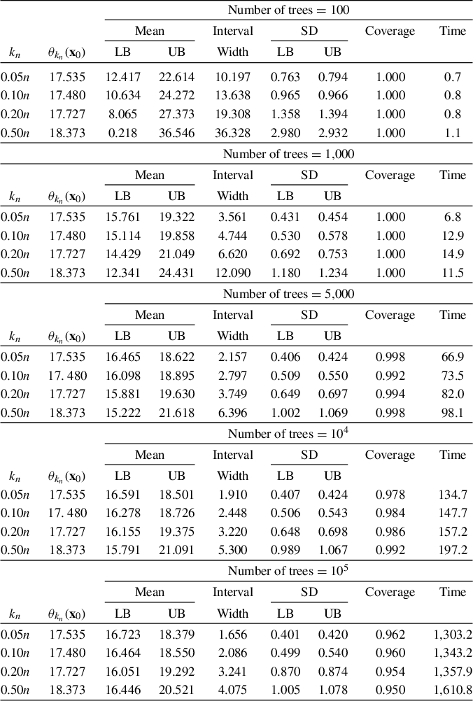

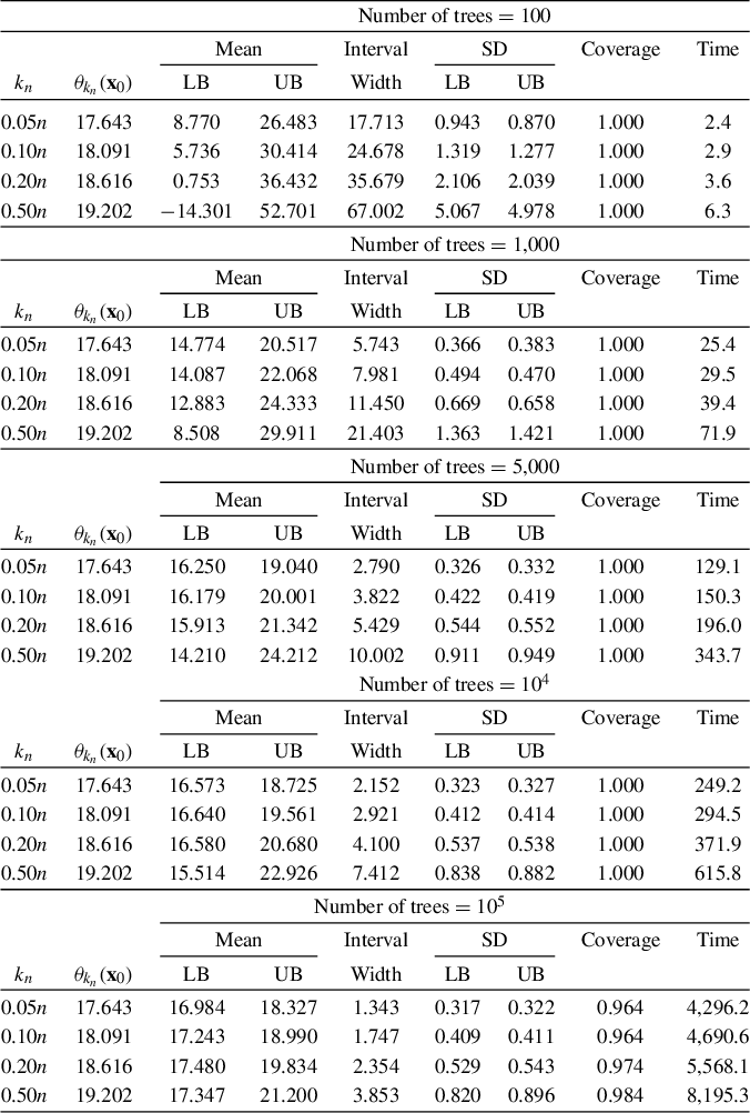

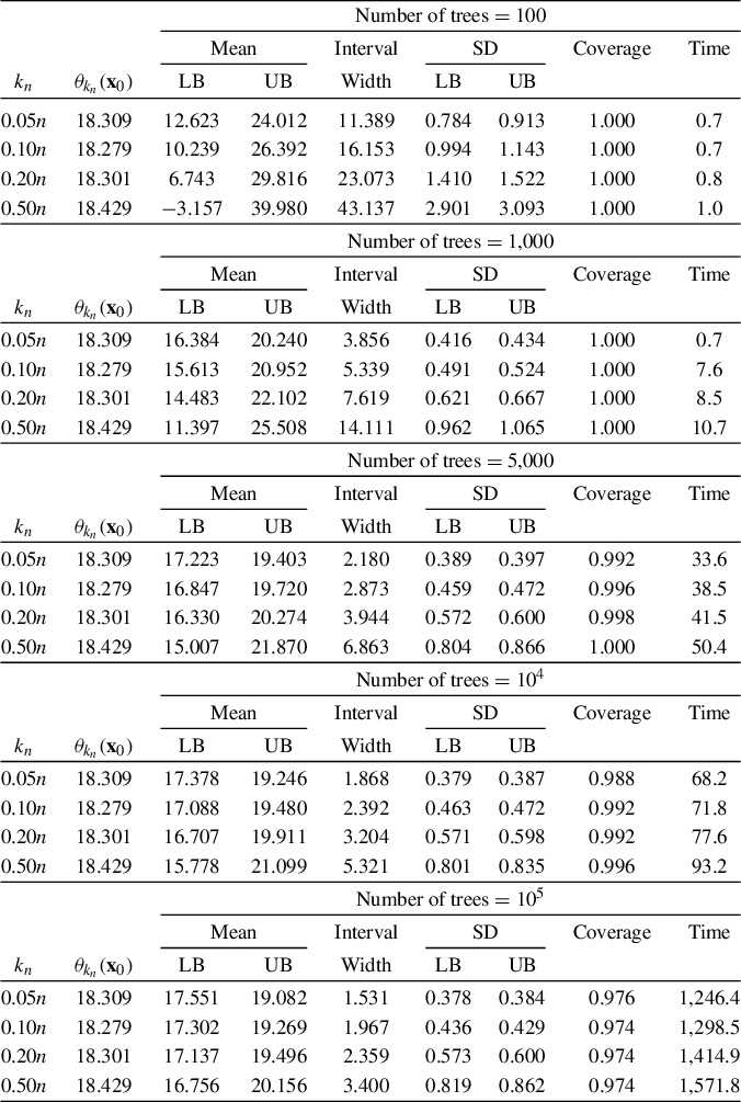

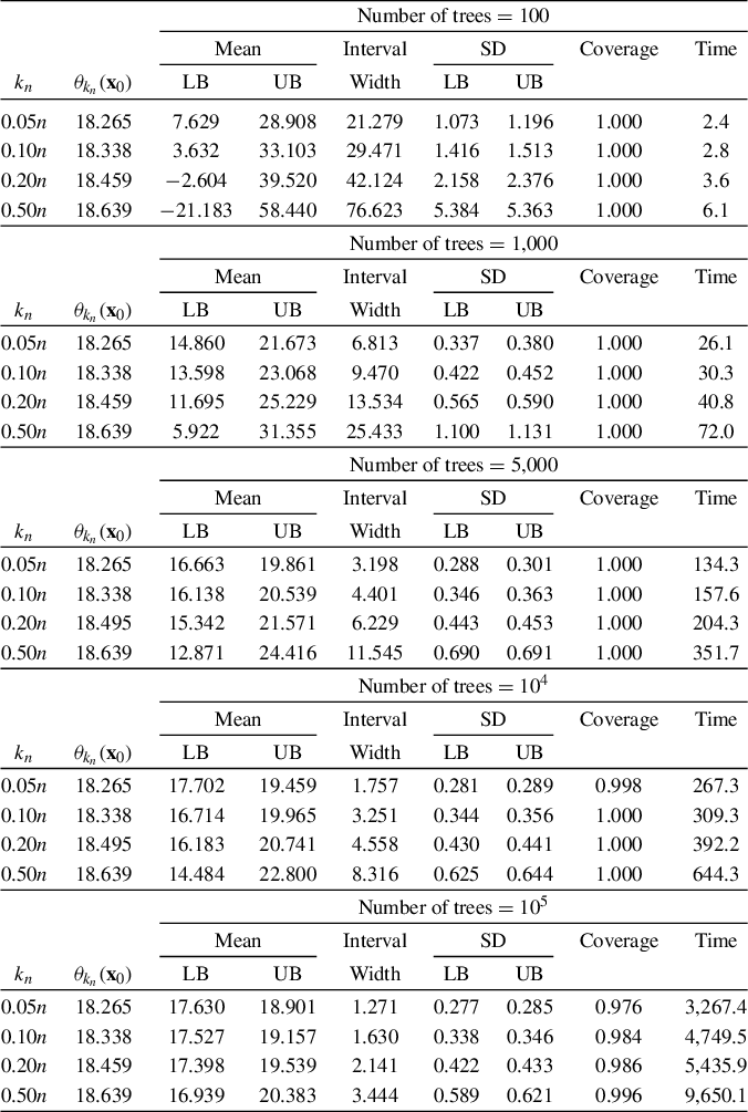

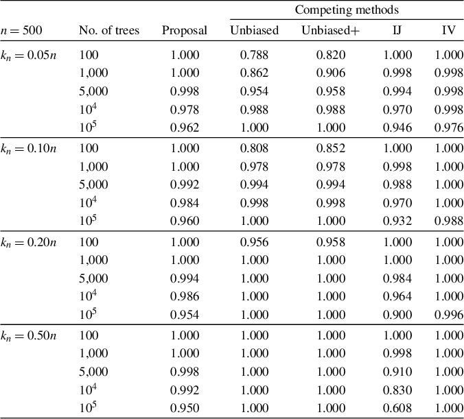
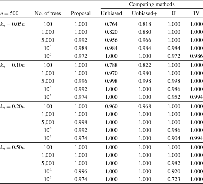
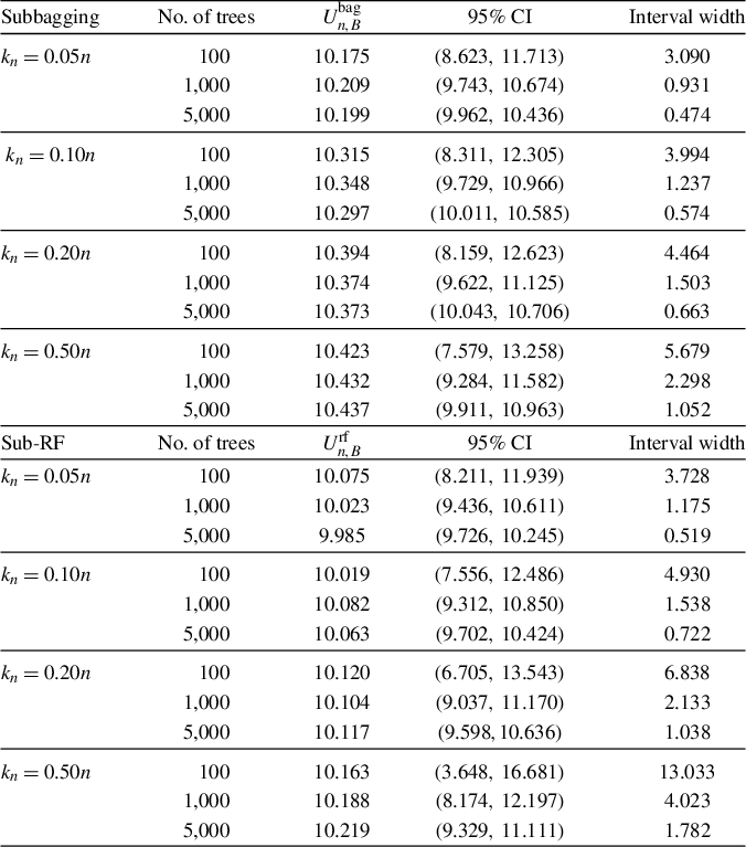

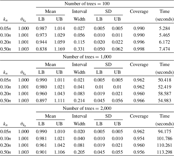

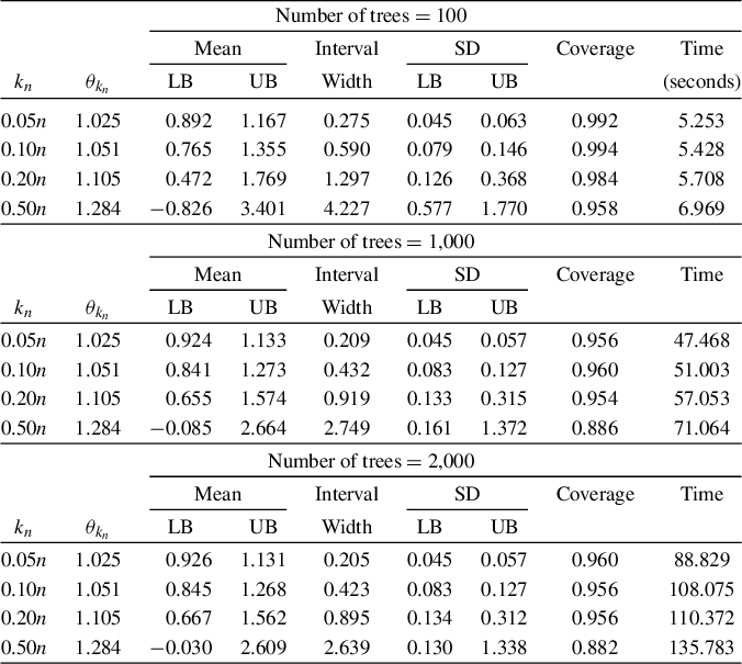


 Open access

