2. A NEW CONCEPT OF PRODUCTION FRONTIER

Let

be the probability space on which the vector of inputs X and the output variable Y are defined. In this approach, we define the attainable set Ψ to be the support of the joint distribution of (X,Y), and we will concentrate on the set Ψ* = {(x,y) ∈ Ψ|F_X(x) > 0}, which contains the interior of Ψ.

From its definition, φ(x), the value of the production function coincides with the order one quantile of the law of Y given X ≤ x,

This suggests introducing a concept of production function of continuous order α ∈ [0,1], as the quantile function of order α of the law of Y given that X does not exceed a given level of inputs. This function takes, for a given level of inputs x, the value

This conditional quantile is the production threshold exceeded by 100(1 − α)% of firms that use less than the level x as inputs. The function F⁻¹(./x) is the so-called generalized inverse of F(·/x). If the distribution function F(·/x) is strictly increasing, its inverse coincides with the generalized inverse F⁻¹(./x). Using this property, we easily obtain the following result.

PROPOSITION 2.1. Assume that for every x such that F_X(x) > 0, the conditional distribution function F(·/x) is strictly increasing on the support [0,φ(x)]. Then,

From property (2), we see that any production unit (x,y) in Ψ* belongs to some α-order quantile curve. Then unit (x,y) produces more than 100α% of all production units using inputs smaller than or equal to x and produces less than the 100(1 − α)% remaining units. Thus the quantile function q_α(x) quantifies the production efficiency of unit (x,y) by comparing it with all units that use the same level of inputs x and also with those that use strictly less than x. This motivates our interest in the distribution of Y given X ≤ x.

But the most attractive property of this quantile function is that it can be easily nonparametrically estimated without the drawbacks of the methods trying to estimate the frontier function itself: it will be less sensitive to noise, extreme values, or outliers. This is developed in the next section.

As it is shown by property (2), the quantile curves {(x,q_α(x))|F_X(x) > 0} cover the whole production set Ψ*. As can be seen in the next proposition, this does not hold for expected order-m frontiers of Cazals et al. (2002) {(x,φ_m(x))|F_X(x) > 0}.

PROPOSITION 2.2. Under the assumption of Proposition 2.1 and if we assume furthermore the free disposability of outputs, i.e.,

then the functions φ_m do not satisfy the following property:

Let us compare how the expected maximal production function and the quantile function can be useful in terms of practical efficiency analysis. Suppose a production unit uses a quantity of inputs x₀ and produces an output y₀; φ_m(x₀) gives the expected maximum production among a fixed number of m firms using less than x₀ as inputs. This value indicates how efficient the unit (x₀,y₀) is, compared with these m units. This is achieved by comparing its level y₀ with the value of φ_m(x₀). For this particular unit, we know that it belongs to a quantile frontier. The order of this frontier, which is known, gives the proportion of units that produce less than y₀ among all firms using less than x₀. Hence the quantile function gives a clearer indication on the production performance, and it can be viewed as a reasonable benchmark value.

We can, however, establish an asymptotic relationship between the two families of production functions φ_m and q_α. Namely, we can state the following proposition.

PROPOSITION 2.3. For every x such that the conditional distribution function F(·/x) is twice differentiable with first derivative f (·/x) strictly positive on the support [0,φ(x)], we have as m → ∞ and α → 1,

where ψ_x′(α) = −F′′(q_α(x)/x)/f³(q_α(x)/x).

From its definition, it is clear that for any fixed x such that F_X(x) > 0, q_α(x) is a monotone nondecreasing function of α. The limiting case when α → 1 is of particular interest. It converges to the efficient frontier: by letting m tend to infinity in (3) and using lim_m→∞ φ_m(x) = φ(x), we obtain φ(x) − q_α(x) = o(α) when α → 1. We can prove this property directly by using the monotonicity of quantiles q_α(x) with respect to α as indicated by the next proposition. Even more strongly it is shown, under some regularity conditions, that the order-α production function q_α converges uniformly to the true production function φ.

PROPOSITION 2.4.

(i) For any fixed value of x such that F_X(x) > 0, we have lim_α→1 [searr] q_α(x) = φ(x).

(ii) Assume that for every α ∈ [0,1], the quantile function q_α(.) is continuous on the interior of the support of X. Then for any compact K interior to the support of X,

The function q_α converges to a monotone nondecreasing function φ as α → 1, but it is not monotone nondecreasing itself unless we add the following assumption:

This assumption is not needed for all the results of this paper except for the next proposition, but it appears to be quite reasonable: it says that the chance of producing less than a value y decreases if a firm uses more inputs. This assumption is necessary and also sufficient.

PROPOSITION 2.5. The quantile function x [map ] q_α(x) is monotone nondecreasing on the set

for every order α ∈ [0,1] if and only if the function x [map ] F(y/x) is monotone nonincreasing on the set

for any output

.

Note that the results established in Proposition 2.4 are very similar to those obtained for the order-m frontier. Indeed φ_m(x) converges simply and uniformly to φ(x) as m → ∞. However for Proposition 2.5, Cazals et al. (2002, Theorem A.3) only prove that if assumption (4) holds then φ_m(x) is monotone nondecreasing in x.

3. NONPARAMETRIC ESTIMATION

To estimate the conditional quantile q_α(x), it is natural to use the conditional empirical quantile obtained by inverting the conditional empirical distribution function

,

This estimator may be computed explicitly as follows. Let N_x be the number of observations X_i smaller than or equal to x, i.e.,

, and, for j = 1,…,N_x, denote by Y_(ij) the jth order statistic of the observations Y_i such that X_i ≤ x: Y_(i1) ≤ Y_(i2) ≤ ··· ≤ Y_(iNx). We have, for x such that N_x ≠ 0,

Hence,

Therefore, we obtain for every α > 0,

where [αN_x] denotes the integral part of αN_x: the largest integer less than or equal to αN_x. The conditional empirical quantile

is thus computed very easily as being the simple empirical quantile of observations y_i such that x_i ≤ x.

For comparison, note that an exact formula is available to compute

. It is as simple as the formula (5) but is restricted to the case of no ties among the inputs. The nonparametric estimator

can also be approximated in practice by using a Monte-Carlo algorithm, even in the full multivariate case (several inputs and several outputs), which we do not treat in our paper. For instance, in the univariate output case, the Monte-Carlo method can be described as follows. For a given x, draw a random sample of size m with replacement among these y_i such that x_i ≤ x and denote this sample by (y_b¹,…,y_b^m). Then compute

. Redo this for b = 1,…,B where B is large. Finally, we have

where the quality of the approximation can be tuned by the choice of B.

Note also that the relation between the order-m frontier and the true frontier remains valid with their estimators

, i.e.,

. Similarly it is easily seen, for any fixed value of inputs x for which the estimator

is well defined for every order α ∈ [0,1], that

is a monotone nondecreasing function of α, and thus

Note that even for large values of α < 1, the estimator

is less sensitive to extreme values than the FDH estimator

, which by construction envelops all the observations. The asymptotic theory is discussed in Section 4. Note also that

is not necessarily monotone nondecreasing with respect to x. Indeed, even if assumption (4) is assumed for the true conditional distribution function, it could happen that its empirical counterpart does not satisfy it. Of course we know that for large sample size n, it will mostly be the case.

Another property that

shares with

lies in the fact that both the nonparametric partial frontiers underestimate the full frontier φ(x), for every order. In our case, for any value of inputs x for which

are well defined for any order α ∈ [0,1], we have

Indeed, because the production function φ(·) is monotone nondecreasing and greater than or equal to the efficient-output function ∂Y(.), for each i such that X_i ≤ x we have almost surely Y_i ≤ ∂Y(X_i) ≤ φ(X_i) ≤ φ(x). Therefore

. On the other hand we have

for every α ∈ [0,1].

4. ASYMPTOTIC PROPERTIES

For the unconditional case where ξ_α denotes the order-α quantile of a distribution function F_Z of a random variable Z, and

denotes the empirical quantile of a sample (Z₁,…,Z_n) of Z, if F_Z is differentiable in ξ_α and such that F_Z′(ξ_α) > 0, the Bahadur representation theorem gives

The direct application of this result to the distribution function F_Z(·) = F(·/x) does not serve our purpose because our data do not yield a sample from this distribution. However, as for unconditional quantiles ξ_α, we focus here on pairs (x,α) that satisfy the following property:

As a consequence of this property, F(·/x) is a bijective transformation from a neighborhood of q_α(x) onto a neighborhood of α. In particular the generalized inverse F⁻¹(·/x) is equal to the inverse of F(·/x) in the neighborhood of α. This property will be used in the proof of the following theorem, which summarizes the asymptotic properties of our estimator

.

THEOREM 4.1. Let α ∈ (0,1) be a fixed order and let x be a fixed value such that F_X(x) > 0. Assume that the conditional distribution function F(·/x) is differentiable at q_α(x) with derivative f (q_α(x)/x) > 0. Then,

where

It is important to note that here, also, the equivalent properties hold with the nonparametric estimator of the order-m frontier. Indeed it is easy to see that

converges at the rate

and is asymptotically unbiased and normally distributed:

, where σ²(x,m) = E [Γ_m²(x,X,Y)], with

Moreover for a vector

, the asymptotic r-variate normal distribution is obtained with asymptotic covariances given by Σ_m(x^k,x^l) = E [Γ_m(x^k,X,Y)Γ_m(x^l,X,Y)]. Similarly we have the following more general result for the estimator of the conditional quantile frontier function.

THEOREM 4.2. Let x¹,…,x^r be r levels of the input X that satisfy the assumption of Theorem 4.1 for a given order α ∈ (0,1). Then,

where

with

In applied work, the variance factors σ²(x,α) and Σ_α(x^k,x^l) must be estimated. For instance, consistent estimators for these factors can be obtained by plugging in nonparametric estimators for the conditional density f (·/x) and the marginal distribution function F_X(x) and taking the empirical mean for the expectation. Note that, as for unconditional quantiles, quantiles in the tail of the conditional distribution where the conditional density is low are inherently more difficult to estimate.

Note also that Cazals et al. (2002) obtained an asymptotic representation for their nonparametric estimator

where the error term is uniform in x, whereas the error term involved in our approach depends on x (see the proof of Theorem 4.1). This can be explained as follows. Both

are representable as functionals of the empirical distribution function

. The corresponding functional for

is differentiable in the Frechet sense w.r.t. the sup-norm, whereas that corresponding to

is only differentiable in the Gâteaux sense. The uniformity of the error term allowed Cazals et al. (2002, Appendix B) to improve the convergence results of

by a functional limit theorem, which is not the case in our approach.

It is also interesting to compare

with the estimator of the standard conditional quantile of the distribution of Y given X = x. First note that this latter estimate requires a smoothing procedure, which is not the case when the distribution of Y is conditioned by X ≤ x. To compare their asymptotic variance, let us recall that the smooth estimators of the quantiles ξ_α(x) of the distribution function F_x of Y given X = x, are obtained by inverting a kernel estimator of F_x and satisfy the following result:

where μ²(x,α) = α(1 − α)R(K)/f_x²(ξ_α(x)), with f_x(y) = (∂/∂y)F_x(y), R(K) = ∫K²(u) du, and K and h_n are, respectively, a kernel and a bandwidth satisfying some specific constraints (see, e.g., Berlinet, Cadre, and Gannoun, 2001; Ducharme, Gannoun, Guertin, and Jequier, 1995).

Let us now turn to the convergence to the full frontier function φ(x). We know that the estimator

converges to the FDH estimator

as α → 1. We also know from Park et al. (2000) that under regularity conditions, as n → ∞, the FDH estimator

converges to the true unknown frontier φ(x). The idea is then to define α as a function of n such that

as n → ∞. We thus derive an estimator of the true production frontier φ(x) and show in the next theorem that it converges to the same asymptotic distribution as the FDH estimator and as the nonparametric envelopment estimator of Cazals et al. (2002). The rate of convergence of the order α(n) to 1 is provided.

THEOREM 4.3. Assume that the joint probability measure of (X,Y) on the compact support Ψ provides a strictly positive density on the frontier {(x,φ(x))|F_X(x) > 0} and that the function φ is continuously differentiable. Then for any x interior to the support of X we have, as n → ∞,

where μ_x is a constant and the order α(n) is such that

The constant μ_x appearing in the limiting Weibull depends on the slope of the frontier and the value of the density near the frontier point (x,φ(x)). A consistent nonparametric estimator of this unknown constant has been proposed in Park et al. (2000).

Like the approach of Cazals et al. (2002), here also we lose the

-consistency because we use

to estimate the full frontier φ(x) and not the partial frontier q_α(x).

5. NUMERICAL ILLUSTRATIONS

In this section, we illustrate our procedure through some numerical examples with simulated and real data. In the simulation study, the observations are simulated according to the same data generating process used in Simar (2003).

5.1. Example 1

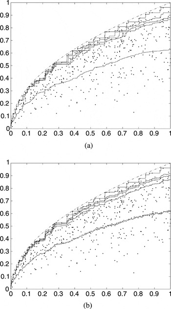
We first consider a situation where the attainable set is convex. We simulate a sample of n = 500 data points (x_i,y_i) according to the Cobb–Douglas log-linear frontier model given by Y = X^0.5 × exp(−U), where X is uniform on (0,1) and U is exponential with mean 1/3. The true frontier function is φ(x) = x^0.5.

Figure 1 illustrates the simulated data and the quantile curves

and the expected maximal frontiers

(B = 1,000) for several different values of α and m. In the solid lines, the estimates

(Figure 1a) with α = 0.7, 0.97, 0.98, 0.99, 1 are compared with the estimates

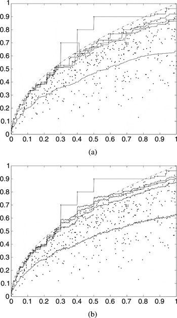
(Figure 1b) with m = 2, 25, 50, 75, ∞. The true frontier φ is in dash-dotted lines. The frontiers are monotone nondecreasing with respect to the order. For Figure 2, we add in the data set three outliers, and we plot the same frontiers

.

n = 500. Comparison between (a) and (b), output vs. input.

n = 503. Comparison between (a) and (b) with three outliers included, output vs. input.

From Figures 1 and 2, it is clear that the frontiers

are more resistant to the three outliers than the FDH frontier, but they are less resistant to the outliers than the quantile frontiers of orders α < 1. Indeed, the quantile frontier

is influenced by only one outlier, and it comes back down immediately, whereas the frontiers

with m = 25, 50, 75 are attracted by all the outliers and moreover continue to grow after each jump. So in this particular example the frontier

is more robust to the outliers than the three frontiers

, whereas it envelops all these frontiers in absence of the three outliers.

5.2. Example 2

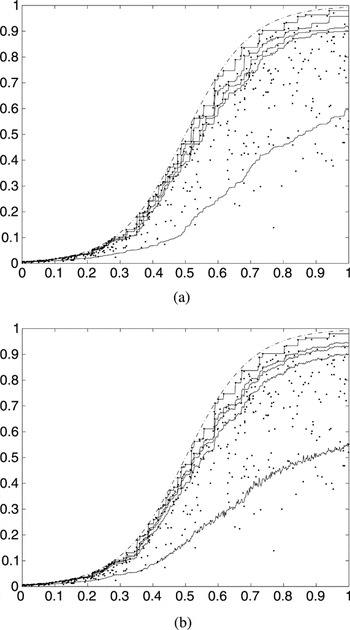
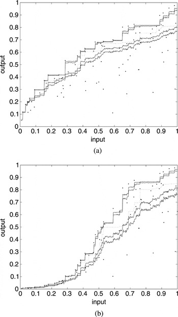
We now simulate a sample of n = 500 data points (x_i,y_i) with a nonconvex production set. We choose here the model Y = exp(−5 + 10X)/(1 + exp(−5 + 10X))exp(−U), where X is uniform on (0,1) and U is exponential with mean 1/3.

Figure 3 plots the simulated data and, in the solid lines, the frontiers

(B = 1,000) with the same orders as in the preceding example and, in the dash-dotted lines, the true frontier φ. Note that, here also, the frontier

is above all the frontiers

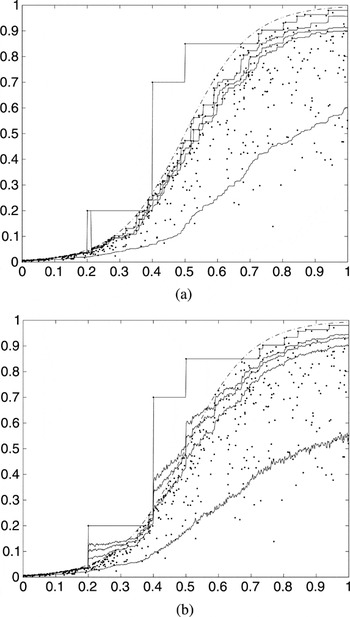
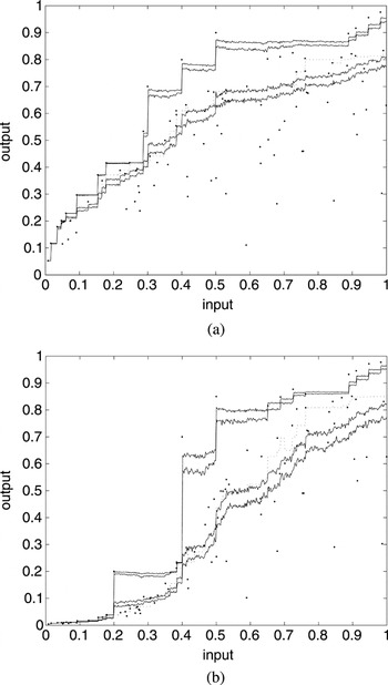
. We again add in the data set three outliers, as shown in Figure 4, and we plot the frontiers

for the same orders. It is clear that the quantile curves of orders α < 1 are more resistant to the three outliers than the expected maximal output frontiers

and the FDH frontier

.

n = 500. Comparison between (a) and (b), output vs. input.

n = 503. Comparison between (a) and (b) with three outliers included, output vs. input.

5.3. Example 3

We now test the robustness of both estimators

for a small sample size n = 100. In Figures 5a and 5b we plot, in the dotted lines, the quantile frontier of order α = 0.93 and, in the solid lines, the frontiers

(B = 1,000) of orders m = 5, 7, 50, 75. In Figure 5a, the data points are simulated according to the same model used in Example 1, and in Figure 5b, they are simulated according to the same model used in Example 2. Observe that the quantile frontier

is below the frontiers

of orders m = 50, 75 and is above those of orders m = 5, 7.

n = 100. In the solid lines, the order-m frontiers and in the dotted lines, the quantile frontier .

In Figure 6 we add to the preceding two data sets the same three outliers used in Examples 1 and 2, and we plot the same frontiers. We remark that the frontiers

of orders m = 50, 75 are highly influenced; even those of very low orders m = 5, 7 are attracted by the three outliers, whereas the quantile frontier is slightly perturbed.

n = 103. In the solid lines, the order-m frontiers and in the dotted lines, the quantile frontier with three outliers included.

We repeated the same exercise with many other simulated data sets, leading to the same kind of results.

5.4. Frontier Analysis of French Post Offices

We examine here a real data set in a univariate situation: this data set about the cost of the delivery activity of the postal services in France is analyzed by Cazals et al. (2002). There are n = 9,521 post offices observed in 1994. For each post office i, the input x_i is the labor cost measured by the quantity of labor, which represents more than 80% of the total cost of the delivery activity. The output y_i is defined as the volume of delivered mail (in number of objects).

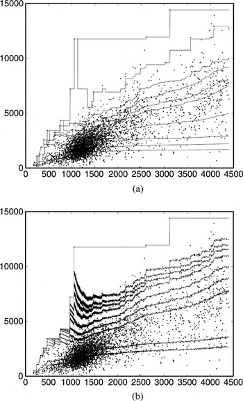
The 4,000 observed post offices with the smallest input levels are plotted in Figure 7, along with the estimates of quantile frontiers (Figure 7a) and of expected maximal output frontiers (Figure 7b), for several different orders α and m. Here we obtain the frontiers

with B = 2,000 bootstrap loops.

The 4,000 observations with the smallest input levels. (a) The frontiers of orders α = 0.3, 0.5, 0.7, 0.9, 0.97, 0.98, 0.99, 0.995, 0.999 and the FDH frontier (α = 1). (b) The frontiers of orders m = 1, 2, 25, 50, 100, 200, 300, 400, 600 and the FDH frontier (m = ∞). Output vs. input.

By using (5), it is very easy to check that every post office i belongs to the quantile curve of order

. On the other hand, the frontiers

do not cover the observations below the first frontier

(12% of the observed data) and the observations between the frontiers of successive orders

. This disadvantage of frontiers

with respect to frontiers

is due to the fact that the order m is discrete.

Note that the order α_i of the quantile frontier that passes through the post office (x_i,y_i) is equal to the percentage of post offices that produce less than y_i among all the post offices using inputs smaller than or equal to x_i. In other words, this order indicates that the ith post office produces more than 100α% of all post offices using inputs smaller or equal to x_i and produces less than the 100(1 − α)% remaining post offices. This is why one sees in Figure 7a that, if α_i is close to one, then the post office (x_i,y_i) can be seen to be performing relatively efficiently, and likewise, if α_i is close to zero, then the post office would be performing relatively inefficiently. Thus the order of the empirical quantile frontier

defines a reasonable benchmark value. Note also that the nonparametric estimation of the expected frontier

can be viewed as a mark of good practice for post offices when studying their performance. However, this benchmark is less clear than the empirical quantile frontier because it is less easy to interpret and does not cover the whole data set.

We also remark that the frontiers

(Figure 7b) are perturbed by the extreme observations from the order m = 25, whereas the frontiers

are not influenced except for those having orders almost equal to one (α ≥ 0.999).

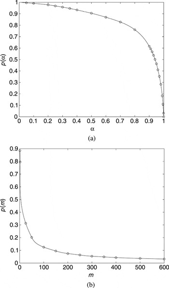
Figure 8a (resp. Figure 8b) indicates how the percentage p(α) (resp. p(m)) of observations above the quantile estimates

(resp. the expected maximum cost estimates

) decreases with α (resp. m). We remark that the percentage p(α) decreases very slowly until the order α = 0.8 of approximately 24% of observations. It means that the quantile frontiers of orders 0 ≤ α ≤ 0.8 are very tight. The 24% observations below the frontier

have an intermediate production performance and can be relatively inefficient. However, the percentage p(α) falls dramatically from the order α = 0.8, which means that the quantile frontiers of extreme orders 0.8 ≤ α ≤ 1 are very spaced and are spread out over 76% of the observations. In particular, 10% of the observations are above the frontier

and 3% of the observations are above the frontier

. It is what explains notably the fact that only quantile frontiers of orders very close to one are influenced by superefficient units.

Evolution of the percentage of observations above the frontiers (a) and (b) .

In Figure 8b, we observe an opposite phenomenon: first the percentage p(m) falls severely until the order m = 50 of approximately 80% of observations, and then it continues to decrease but very slowly. Consequently the frontiers

of orders m ≥ 50 are very tight. In particular we just have 9% of observations between the two frontiers

, and only 3% of observations are above the frontier

. The 20% observations above the frontier

are extreme and could be outliers or noisy observations. In summary the frontiers

are very tight from the order m = 50 and are spread out over extreme observations; it is then natural that these frontiers would be more sensitive to extreme values than the quantile frontiers.

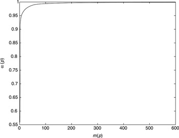
We can illustrate this result more clearly by considering the following inverse problem: for a given percentage p₀, denote by α(p₀) (resp. m(p₀)) the order of the frontier

(resp.

) above which the percentage of observations is equal to p₀; we have p(α(p₀)) = p(m(p₀)) = p₀. Inverting the relationship between α and p(α) and between m and p(m) in Figure 8, we get the evolution of α and m as functions of p. When the percentage p varies between 0 and 10%, we remark that the order α(p) is almost constant (α(p) ≈ 1), whereas the order m(p) falls rapidly from m = 600 to m ≈ 100. This means that the 10% extreme observations influence all the frontiers

with orders 100 ≤ m ≤ ∞, whereas only the frontiers

with orders almost equal to 1 are influenced by these extreme observations. This can be understood because the FDH frontier

envelops all the observed data.

This result is also illustrated in Figure 9, where the curve of evolution of α(p) with respect to m(p) is nearly flat from the point (100, 0.995) which corresponds to the percentage p ≈ 10%. This plot establishes an empirical relationship between the two families of frontiers

. Given a frontier

, we can determine the frontier

above which we have the same percentage of observations and vice versa.

An empirical relationship between .