


1. INTRODUCTION
In an important contribution to the literature, Phillips and Solo (Reference Phillips and Solo1992)—hereafter, PS92—provided a number of asymptotic results for normalized sums of discrete-time linear processes (DTLPs) that satisfy certain innovation properties as well as summability conditions on the coefficients. Their results have subsequently been used by many authors owing to their wide applicability and relative ease of use. In many instances, however, it may be more appropriate to regard discrete-time observations as having been generated by some underlying process in continuous time. If this continuous-time process also has a representation as a linear process, a natural question to ask is: under what conditions on the continuous-time linear process (CTLP) can the results of PS92 be applied to the discrete-time observations?
A similar question was earlier addressed by Hansen and Sargent (Reference Hansen, Sargent, Hansen and Sargent1991) and Marcet (Reference Marcet, Hansen and Sargent1991). They examine the relationship between CTLPs and DTLPs and show that, in general, the innovations in the DTLP implied by the CTLP will be serially correlated. This immediately rules out direct application of the PS92 results for the discretely-sampled continuous-time process owing to PS92 requiring the innovations to be at least serially uncorrelated in the majority of their results. Furthermore, Hansen and Sargent (Reference Hansen, Sargent, Hansen and Sargent1991) show that, in a multivariate setting, it is only continuous-time processes having a first-order autoregressive (AR) discrete-time representation that have serially uncorrelated innovations in the DTLP representation, a feature that would appear to severely limit the application of the PS92 results to continuous-time processes sampled in discrete time. However, as we demonstrate below, the class of eligible processes is actually somewhat broader, extending to more general finite-order continuous-time AR (CAR) and CAR moving average (CARMA) processes.
The estimation of the parameters of CAR and CARMA processes from discretely-sampled data is a well-established topic in the econometrics and statistics literatures. Time domain likelihood approaches based on an exact discrete-time representation of the CAR process can be found in Bergstrom (Reference Bergstrom1983) and Chambers (Reference Chambers1999), for example, while a state space representation allied to the Kalman filter, such as in Harvey and Stock (Reference Harvey and Stock1985), provides an alternative likelihood-based approach in the time domain. The state space approach can, of course, also be adapted to CARMA systems, as in Zadrozny (Reference Zadrozny1988), while Robinson (Reference Robinson and Phillips1993) advocates an alternative method based in the frequency domain. Exact discrete-time representations can also be derived for CARMA systems, as in Chambers and Thornton (Reference Chambers and Thornton2012), and CARMA processes driven by a Lévy process have been examined by Brockwell (Reference Brockwell, Rao and Shanbhag2001, Reference Brockwell2004). Although much has been done in terms of methods for estimating continuous-time systems using discretely-sampled data, there has been less focus on the asymptotic properties of such data, and the results contained here provide a contribution in that regard.
Our starting point is a multivariate continuous-time state-space representation consisting of a transition equation and a measurement equation that is capable of representing CAR(p) and CARMA(p, q) processes, that is, CAR processes of order p and CARMA processes of orders p and q for finite p and q. The state vector, which contains unobservable components for
$p>1$
 , satisfies a first-order AR process in discrete time and hence, using the Hansen and Sargent (Reference Hansen, Sargent, Hansen and Sargent1991) insight, has a DTLP representation with serially uncorrelated innovations. This forms the basis for application of the PS92 results.
We consider two types of observations, namely, stocks (which are skip-sampled) and flows (which are observed as integrals). In the case of stocks, the observations are linear combinations of the discretely-sampled state vector which are captured by the measurement equation in the state space representation. We derive CTLPs for the state vector and the continuous-time stock process and a DTLP for the discretely-sampled state vector.Footnote 1 We derive laws of large numbers (LLNs), central limit theorems (CLTs), and invariance principles (IPs) for the levels and squares of the observed stock variable by verifying that the required conditions are satisfied for application of multivariate versions of the PS92 results. Underlying much of this is the Beveridge–Nelson (BN) decomposition as in PS92, albeit in a multivariate form.
For flow variables, on the other hand, it is necessary to examine the properties of integrals (over the observation interval) of the underlying state vector, a linear combination of which yields the observed flow. An interesting feature that emerges in the DTLP for the discretely-sampled integrated state vector is the presence of a serially uncorrelated component in addition to the linear process itself. It transpires that it is sums of this additional component that drive the asymptotics in the BN representation owing to the long-run matrix that multiplies the usual innovations being null in this case. As in the case of stocks, multivariate versions of the PS92 results applied to the discretely-sampled integrated state vector yield LLNs, CLTs, and IPs for the levels and squares of the observed flow by considering the appropriate linear combination.
The outline is as follows. Section 2 defines the continuous-time state-space representation of a CAR(p) or CARMA(p, q) process and focuses on the discrete-time sampling of a stock variable. Theorem 1 provides appropriate CTLPs and DTLPs that drive subsequent results. Proposition 1 verifies the relevant summability conditions in terms of matrix norms that enable multivariate versions of the PS92 results to be applied, from which the LLNs, CLTs, and IPs are obtained (Theorem 2). The same approach is applied in Section 3 but this time the object of interest is the integral of the state vector, a linear combination of which yields the flow process. Section 4 provides a unit (zero) root testing example to show how the preceding results can be applied, with Section 5 concluding. All main proofs are presented in the Appendix with some additional results contained in the Supplementary Material.
In terms of notation,
$\stackrel {a.s.}{\rightarrow }$
 denotes almost sure convergence;
$\stackrel {d}{\rightarrow }$
 denotes convergence in distribution;
$[x]$
 denotes the integer part of a real number x;
$W(r)$
 is a Wiener (standard Brownian motion) process on
$r\in [0,1]$
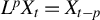
 ; i.i.d. stands for independent and identically distributed; and L is the lag (or backshift) operator such that, for a discrete-time variable
$X_t$
 ,
$L^pX_t=X_{t-p}$
 . In addition, for a
$p\times q$
 matrix B with elements
$B_{ij}$
 ,
$\|B\|=(\sum _{i=1}^p\sum _{j=1}^qB_{ij}^2)^{1/2}$
 , while for a
$p\times p$
 matrix A,
$\mbox {tr}\{A\}=\sum _{i=1}^pA_{ii}$
 denotes the trace and

denotes the matrix exponential,
$I_p$
 denoting the
$p\times p$
 identity matrix. Furthermore,
 denotes column p of the matrix A, while
$o_{a.s.}(1)$
 denotes a random quantity that converges almost surely to zero. Finally, the sampling interval is denoted h and the sample size n with all asymptotic results obtained letting
$n\rightarrow \infty $
 with h fixed.
2. THE MODEL AND DISCRETE-TIME SAMPLING OF A STOCK VARIABLE
The model considered by PS92 is the DTLP given by

where
$C(z)=\sum _{j=0}^\infty c_jz^j$
 with
$0<|C(1)|<\infty $
 ,

and
$\epsilon _t$
 is an i.i.d. innovation process satisfying various moment conditions (the
$\mathcal {A}$
 and
$\mathcal {C}$
 conditions in PS92). PS92 also consider situations in which
$\epsilon _t$
 is a martingale difference sequence (their
$\mathcal {B}$
 conditions) but we will focus on the i.i.d. assumption here. PS92 demonstrate how various summability properties for the coefficients
$c_j$
 , as well as the different moment conditions for the innovations
$\epsilon _t$
 , can be utilized to derive a number of asymptotic results (such as LLNs, CLTs, and IPs) regarding normalized sums of
$X_t$
 and
$X_t^2$
 (both being our focus here) as well as other quantities of interest.
The analysis of finite variance covariance stationary linear processes in continuous time has a long history in the time series literature. Following, for example, Rozanov (Reference Rozanov1967, Thm. 3.1) and Hannan (Reference Hannan1970, p. 155), such processes, for a variable
$X(t)$
 , can be written

where
$\theta (\cdot )$
 is a real-valued kernel (or weighting) function satisfying

while
$\zeta (dt)$
 is an uncorrelated random measure satisfying the following assumption.
Assumption 1. The random measure
$\zeta (dt)$
 satisfies: (i)
$E(\zeta (dt))=0$
 ; (ii)
$E(\zeta (dt)^2)=\sigma ^2dt$
 ; and (iii)
$E(\zeta (\Delta _1) \zeta (\Delta _2))=0$
 for disjoint intervals
$\Delta _1$
 and
$\Delta _2$
 .
Further details regarding random measures can be found in Rozanov (Reference Rozanov1967) as well as Bergstrom (Reference Bergstrom, Griliches and Intriligator1984). Alternative, stronger, and conditions regarding
$\zeta (dt)$
 are used later in Theorems 2 and 4 when applying the PS92 results.
Ideally, it would be possible to proceed with the generality of the CTLP (3) and relate the
$c_j$
 coefficients in the DTLP (1) to the weighting function
$\theta (\cdot )$
 . Although this can, in fact, be done, the resulting innovations (
$\epsilon _t$
 ) in (1) aren’t, in general, i.i.d., but instead exhibit correlations over time. Hansen and Sargent (Reference Hansen, Sargent, Hansen and Sargent1991) and Marcet (Reference Marcet, Hansen and Sargent1991) show that from (1) we can write

where, writing
$C(z)^{-1}=\sum _{j=0}^\infty \gamma _jz^j = \gamma (z)$
 ,

The implication is that, in general,
$\epsilon _t$
 will depend on the entire past history of
$\zeta (dt)$
 and is, therefore, serially correlated.
Hansen and Sargent (Reference Hansen, Sargent, Hansen and Sargent1991) investigate circumstances in which
$\epsilon _t$
 will be uncorrelated and consider what they regard as the “ideal” form given by

so that
$\epsilon _t$
 only depends on
$\zeta (dt)$
 over the unit time interval and, moreover, the weighting function is given by
$\theta (r)$
 . They are able to show that it is only continuous-time processes with first-order discrete-time representations that have innovations of this form, which appears to restrict the class of continuous-time processes to which the PS92 results can be applied. However, we demonstrate below, in Theorem 1, that the class of eligible processes is somewhat broader, extending to finite-order CAR(p) and CARMA(p, q) processes.
Our focus here, then, is on a variable,
$X(t)$
 , that evolves in continuous time as either a CAR(p) or a CARMA(p, q) process. In the case of a CAR(p) process, we have

where D denotes the mean square differential operator,
$a_0,a_1,\ldots ,a_{p-1}$
 are real-valued coefficients, and
$\zeta (dt)$
 satisfies Assumption 1.
Extending (5) in the natural way to allow for MA(q) errors results in an equation whose disturbance term contains components of the form
$D^j\zeta (dt)$
 for
$j=1,\ldots ,q$
 , but this is problematical owing to derivatives of
$\zeta (dt)$
 not being well-defined. However, Brockwell (Reference Brockwell, Rao and Shanbhag2001, Reference Brockwell2004) shows that a valid representation of a CARMA(p, q) process (for
$p>q$
 )Footnote
2
is given by a state space form consisting of the transition equation

where

and the measurement equation

where
$b_j (j=1,\ldots ,p-1)$
 denote the MA coefficients with
$b_j=0$
 for
$j>q$
 . The CAR(p) is obtained as a special case by setting
$b_1=b_2=\cdots =b_{p-1}=0$
 . In the CAR(p) case, it is the first element of
$Y(t)$
 that is of interest whereas in the CARMA(p, q) case interest centers on a linear combination of (potentially all of) the elements of
$Y(t)$
 .
We make the following assumption regarding the roots of the characteristic equation of the companion matrix A in (6).
Assumption 2. The roots of the equation
$\lambda ^p - a_{p-1}\lambda ^{p-1} - \cdots - a_1\lambda - a_0 = 0$
 are distinct and have negative real parts.
Assumption 2 ensures that the process
$Y(t)$
 is covariance stationary. It would be possible to allow for repeated roots albeit at the cost of greater notational complexity but little of real substance would be gained by doing so. As the coefficients of the characteristic equation are real, the characteristic roots will also either be real or they will occur in complex conjugate pairs. It is convenient, for some of what follows, to assign the real roots to the first
$p_1$
 eigenvalues, followed by the
$p_2$
 distinct complex eigenvalues and then their
$p_2$
 conjugates, which gives (with
$i^2=-1$
 )

so that
$p=p_1+2p_2$
 ; if
$p_1=0$
 (or
$p_2=0$
 ) then all roots are complex (or real). The companion matrix A then has the decomposition

where
$\Lambda $
 is a diagonal matrix with the
$\lambda _k$
 on the diagonal and P is a matrix whose columns are the eigenvectors corresponding to the eigenvalues. The exponential of A, which is needed in what follows, also has the convenient representation

where
$e^\Lambda $
 is a diagonal matrix with
$e^{\lambda _k}$
 on the diagonal. It is also convenient, notationally, to define the
$p\times p$
 matrix function

using this notation,
$e^A=\Theta (1)$
 .
In the remainder of this section, we shall assume that
$X(t)$
 is a stock variable whose skip-sampled version at regular time intervals of length
$h>0$
 is given by the sequence

With this in mind, the discrete-time measurement equation is

where
$Y_{th}=Y(th)$
 . From (6),
$Y(t)$
 has the solution

where we note that post-multiplication of
$e^A$
 by
$e_p$
 picks out the last column (p) of that matrix. Further, by splitting the integral on the right, it is straightforward to show that
$Y_{th}$
 has the VAR(1) representation

these representations form the basis for the following result.
Theorem 1. Let the continuous-time process
$Y(t)$
 satisfy (6). Then, under Assumptions 1 and 2:
(a)
$Y(t)$
 has the CTLP representation

where
$\tilde \zeta (dt)=e_p\zeta (dt)$
 and

(b)
$X(t)$
 has the CTLP representation

where
 and

(c)
$Y_{th}$
 has the DTLP representation

where
$C_{h,j} = e^{Ahj}$
 and
$\epsilon _{th}$
 , which is defined in (14), is an uncorrelated
$p\times 1$
 vector process with mean zero and covariance matrix

The coefficient matrices in the linear process (15) satisfy
$C_{h,0}=I_p$
 ,

where
$\kappa (P)=\|P\|\|P^{-1}\|\geq 1$
 is the condition number of P.
Theorem 1 has three components. Part (a) shows that the continuous-time process
$Y(t)$
 , satisfying (6), has a valid CTLP representation with square-integrable norms for the matrix filter function. Part (b) shows that the process of interest,
$X(t)$
 , which is a linear combination of
$Y(t)$
 , also has a valid CTLP representation with square-integrable weighting function. The final part, (c), presents the DTLP representation for
$Y_{th}$
 and demonstrates the square-summability of the matrix norms in this representation as well as providing an upper bound for the individual matrix norms themselves.
A conspicuous absence from Theorem 1 is a result containing a DTLP for the observed process
$X_{th}=b'Y_{th}$
 . In view of
$X_{th}$
 being covariance stationary, a Wold representation certainly exists but the challenge here is relating its coefficients and innovations back to the underlying continuous-time processes,
$X(t)$
 or
$Y(t)$
 . Essentially what would be required is a result for a linear combination,
$X_{th}=b'Y_{th}$
 , of the elements of a multivariate MA(
$\infty $
 ) process,
$Y_{th}$
 . Results that exist tend to focus on the resulting order of the contemporaneously aggregated process rather than the relationship between the coefficients and also concentrate on finite-order VARMA(p, q) processes (see, e.g., Lütkepohl, Reference Lütkepohl1987, Reference Lütkepohl2005).
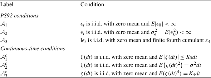
In order to utilize the PS92 results, it is necessary to verify that the relevant innovation and summability conditions are satisfied. In the case of the former, Table 1 contains the relevant PS92 innovation conditions and the corresponding continuous-time conditions relating to
$\zeta (dt)$
 which represent a strengthening of Assumption 1. The continuous-time conditions contain a superscript “c” so that, for example,
$\mathcal {A}_1^c$
 is the continuous-time counterpart to the PS92 condition
$\mathcal {A}_1$
 for DTLPs. In the absence of a DTLP, for observations on
$X(t),$
 we have to rely instead on properties of the vector DTLP for
$Y_{th}$
 and then relate them to
$X(t)$
 . The required summability conditions on the coefficient matrices
$C_{h,j}$
 are contained in the following proposition.
Proposition 1. Let
$Y(t)$
 satisfy (6) so that
$Y_{th}$
 has the DTLP representation (15) with coefficient matrices
$C_{h,j}=e^{Ahj}$
 . Then, under Assumption 2:

Innovation conditions

Table 1 Long description
The table is divided into two main sections.
Section 1: P S 9 2 conditions.
- Label A sub 1: epsilon sub t is i.i.d. with zero mean and E absolute value of epsilon sub 0 is less than infinity.
- Label A sub 2: epsilon sub t is i.i.d. with zero mean and sigma sub epsilon squared equals E of epsilon sub 0 squared which is less than infinity.
- Label A sub 3: epsilon sub t is i.i.d. with zero mean and finite fourth cumulant kappa sub 4.
Section 2: Continuous-time conditions.
- Label A sub 1 super c: zeta (d t) is i.i.d. with zero mean and E of absolute value of zeta (d t) is less than or equal to K sub 0 d t.
- Label A sub 2 super c: zeta (d t) is i.i.d. with zero mean and E of zeta (d t) squared equals sigma squared d t.
- Label A sub 3 super c: zeta (d t) is i.i.d. with zero mean and E of zeta (d t) to the fourth power equals K sub 4 d t.
A footer note specifies that in conditions A sub 1 super c through A sub 3 super c, the constants K sub 0, sigma squared, and K sub 4 are all finite.
Note: In
$\mathcal {A}_1^c$
 –
$\mathcal {A}_3^c$
 , the constants
$K_0$
 ,
$\sigma ^2$
 , and
$K_4$
 are all finite.
The numbering of these summability conditions conforms to the numbering in PS92; they are used in the proof of Theorem 2 below. Of particular note is the fact that no further restrictions are required on the parameters of (6) and (7) in order for the required summability conditions to hold.
We shall now consider a finite sample of skip-sampled observations of the form

where n denotes the sample size. It is convenient to write the linear process (15) in the form

This representation is particularly useful for the BN decomposition of
$Y_{th}$
 given by

where

(see PS92 (p.976)). As shown by PS92, the BN decomposition is particularly useful in deriving asymptotic results for sums of the variable of interest, such as

because they can typically be based on results for sums of the uncorrelated process
$\epsilon _{th}$
 provided
$\tilde \epsilon _0$
 and
$\tilde \epsilon _{nh}$
 are asymptotically negligible, while from Theorem 1(c),

The results in PS92, suitably modified for the multivariate nature of
$Y_{th}$
 , enable the following results to be determined.
Theorem 2. Let
$X_{th}$
 satisfy (12) and let
$Y(t)$
 satisfy (6). Then, under Assumptions 1 and 2 and the additional conditions stated below, as
$n\rightarrow \infty $
 , the discrete-time sample (17) satisfies the following properties:
(a) If either
$\mathcal {A}_1^c$
 or
$\mathcal {A}_2^c$
 holds, then

(b) If
$\mathcal {A}_2^c$
 holds, then

where
$\sigma _h^2 = b'C_h(1)\Omega _h C_h(1)'b$
 .
(c) If
$\mathcal {A}_2^c$
 holds, then

(d) If
$\mathcal {A}_3^c$
 holds, then

where

and
$K_4$
 is defined in Table 1.
Theorem 2 provides a useful set of asymptotic results for discrete-time samples of stock variables that are justified by conditions on the innovation in the underlying continuous-time process in (6); no further assumptions are required on the process beyond Assumption 2 as it has been shown in Proposition 1 that the required summability conditions on the DTLP are satisfied under this assumption. A potential application of the results in Theorem 2 is provided in Section 4.
3. DISCRETE-TIME SAMPLING OF A FLOW VARIABLE
Not all variables can be observed in the same way as stock variables so the sample that a researcher is faced with may be different from that represented in (17). In this section, we will investigate how, if at all, the conditions underpinning the asymptotic results might change when the discrete-time sample represents observations on a flow variable.
The temporal aggregation process that yields a flow variable is of the form

where

The sequence of discrete-time values of interest for a flow variable are the skip-sampled values of
$X^f(th)$
 , that is,

where
$Y_{th}^f$
 denotes the skip-sampled values of
$Y^f(th)$
 . The analog of Theorem 1 for flow variables is presented below.
Theorem 3. Let the continuous-time process
$Y(t)$
 satisfy (6). Then, under Assumptions 1 and 2:
(a)
$Y^f(th)$
 has the CTLP representation

where

and
$\tilde \zeta (dt)$
 is defined in Theorem 1(a).
(b)
$X^f(th)$
 has the CTLP representation

where
 and

(c)
$Y_{th}^f$
 has the DTLP representation

where

are uncorrelated random disturbances with zero means and covariance matrices

respectively,
$B_{h,0}=I_p$
 ,
$B_{h,j} = C_{h,j}-C_{h,j-1} (j=1,2,\ldots )$
 ,

where
$\lambda _h = p^{1/2}+\kappa (P)\left (2\sum _{k=1}^{p_1+p_2}e^{2hr_k}\right )^{1/2}$
 and
$\kappa (P)$
 is defined in Theorem 1(c).
Theorem 3 shows that, although the temporal aggregation inherent in flow variables affects the precise form of the LP representations, the substantive properties of the representations remain broadly unchanged, with one exception. That is, the process
$Y^f(th)$
 has a CTLP representation with weighting matrix function having square-integrable norm, the scalar process of interest,
$X^f(th)$
 , also has a CTLP representation with square-integrable weighting function, while the vector process
$Y_{th}^f$
 , from which the observed flows are obtained, has a DTLP representation whose weighting matrices are bounded and square-summable. The exception manifests itself in the additional uncorrelated disturbance term,
$\eta _{th}$
 , in the DTLP representation for
$Y_{th}^f$
 , and its presence is important in the derivation of the asymptotic distributions in Theorem 4 below.
The matrix weighting function in the CTLP representation of
$Y^f(th)$
 is more complicated than in the case of a stock variable as it involves integrals of
$\Theta (r)$
 —this arises solely due to the integration inherent in a flow variable. It is also worth noting in passing that the DTLP representation for
$Y_{th}^f$
 in Theorem 3(c) can be obtained in at least four different ways. The proof provided in Appendix A is based on integrating (6) over
$(th-h,th]$
 , yielding the integral on the right-hand side and the difference
$Y(th)-Y(th-h)$
 on the left, and then using the DTLP in Theorem 1(c) for
$Y(th)$
 and its lag. Alternatively, it is possible to obtain the same result by integrating (14); by integrating, the DTLP in Theorem 1(c) directly; or by integrating, the equation

over
$s\in (th-h,th]$
 , as in the state space approaches of Harvey and Stock (Reference Harvey and Stock1988) and Zadrozny (Reference Zadrozny1988). All four methods yield the same DTLP in Theorem 3(c).
In Theorem 3(c), the disturbance terms,
$\xi _{th}$
 and
$\eta _{th}$
 , both involve the inverse of the companion matrix A. The determinant of A is equal to
$(-1)^{p+1}a_0$
 which is clearly nonzero.Footnote
3
If we write A in the form

where
$a'=(a_1,a_2,\ldots ,a_{p-1})$
 , it is straightforward to show that

In terms of the definition of
$\eta _{th}$
 , which involves
$A^{-1}e_p$
 (the last column of
$A^{-1}$
 ), this implies that

Furthermore, as
$X_{th}^f=b'Y_{th}^f$
 , we will need to consider
$b'\eta _{th}$
 which is simply

Note that, under Assumption 1,
$\zeta _{th}$
 is an uncorrelated zero mean process with variance
$\sigma ^2h$
 .
The sample of observations of the flow variable is of the form

where, as before, n denotes the sample size. In what follows, it is convenient to express (21) in the form

An interesting property of this representation manifests itself when we consider the BN decomposition given by

where, analogously to the stock case,

There are two features of this representation that warrant highlighting. The first is the presence of the uncorrelated term
$\eta _{th}$
 in addition to the usual components. The second is not immediately obvious but concerns the term
$B_h(1)$
 . Given that
$B_{h,j} = C_{h,j}-C_{h,j-1}$
 and
$B_{h,0}=C_{h,0}=I_p$
 , we find that

and hence, the BN decomposition becomes

It follows that sums of
$Y_{th}^f$
 , for example, are of the form

so that it is suitably-normalized sums of
$\eta _{th}$
 , rather than of
$\xi _{th}$
 , that determine the asymptotics (assuming that
$\tilde \xi _0$
 and
$\tilde \xi _{nh}$
 are asymptotically negligible).
In order to use the PS92 results with a flow variable, it is necessary to verify that the required summability conditions apply for the DTLP in Theorem 3(c). This, in fact, follows straightforwardly from Proposition 1 and the bound relating
$\|B_{h,j}\|$
 to
$\|C_{h,j}\|$
 , resulting in the following proposition.
Proposition 2. Let
$Y(t)$
 satisfy (6) so that
$Y_{th}^f$
 has the DTLP representation (21) with coefficient matrices
$B_{h,j}$
 defined in Theorem 3(c). Then, under Assumption 2,

The numbering of these summability conditions once again conforms to the numbering in PS92, and an “f” superscript is used to distinguish them from those in Proposition 1. The asymptotic results in the case of a flow variable are presented in Theorem 4.
Theorem 4. Let
$X_{th}$
 satisfy (19) and let
$Y(t)$
 satisfy (6). Then, under Assumptions 1 and 2 and the additional conditions stated below, as
$n\rightarrow \infty $
 , the discrete-time sample (22) satisfies the following properties:
(a) If either
$\mathcal {A}_1^c$
 or
$\mathcal {A}_2^c$
 holds, then

(b) If
$\mathcal {A}_2^c$
 holds, then

where
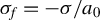
$\sigma _f = -\sigma /a_0$
 .
(c) If
$\mathcal {A}_2^c$
 holds, then

where

(d) If
$\mathcal {A}_3^c$
 holds, then

where

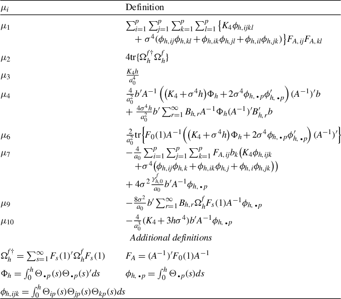
and the
$\mu _i$
 quantities are defined in Table 2.
Definitions of
$\mu _i$
 quantities in Theorem 4

Table 2 Long description
The table is organized into two columns: the left column lists the variable name and the right column provides its mathematical definition.
* mu sub 1: Summation from i equals 1 to p, summation from j equals 1 to p, summation from k equals 1 to p, summation from l equals 1 to p of the quantity { K sub 4 phi sub h,ijkl + sigma super 4 (phi sub h,ij phi sub h,kl + phi sub h,ik phi sub h,jl + phi sub h,il phi sub h,jk) } F sub A,ij F sub A,kl.
* mu sub 2: 4 trace { Omega sub h super f dagger Omega sub h super f }.
* mu sub 3: K sub 4 h all over a sub 0 super 4.
* mu sub 4: 4 all over a sub 0 squared b prime A inverse ((K sub 4 + sigma super 4 h) Phi sub h + 2 sigma super 4 phi sub h, dot p phi sub h, dot p prime ) (A inverse) prime b + 4 sigma super 4 h all over a sub 0 squared b prime summation from r equals 1 to infinity B sub h,r A inverse Phi sub h (A inverse) prime B sub h,r prime b.
* mu sub 6: 2 all over a sub 0 squared trace { F sub 0 (1) A inverse ((K sub 4 + sigma super 4 h) Phi sub h + 2 sigma super 4 phi sub h, dot p phi sub h, dot p prime ) (A inverse) prime }.
* mu sub 7: minus 4 all over a sub 0 summation from i equals 1 to p summation from j equals 1 to p summation from k equals 1 to p F sub A,ij b sub k (K sub 4 phi sub h,ijk + sigma super 4 (phi sub h,ij phi sub h,k + phi sub h,ik phi sub h,j + phi sub h,i phi sub h,jk) ) + 4 sigma squared gamma sub h,0 super f all over a sub 0 b prime A inverse phi sub h, dot p.
* mu sub 9: minus 8 sigma squared all over a sub 0 b prime summation from r equals 1 to infinity B sub h,r Omega sub h super f F sub s (1) A inverse phi sub h, dot p.
* mu sub 10: minus 4 all over a sub 0 cubed (K sub 4 + 3 h sigma super 4) b prime A inverse phi sub h, dot p.
Additional definitions at the bottom include:
* Omega sub h super f dagger: Summation from s equals 1 to infinity F sub s (1) prime Omega sub h super f F sub s (1).
* F sub A: (A inverse) prime F sub 0 (1) A inverse.
* Phi sub h: Integral from 0 to h of Theta sub dot p (s) Theta sub dot p (s) prime d s.
* phi sub h, dot p: Integral from 0 to h of Theta sub dot p (s) d s.
* phi sub h,ijk: Integral from 0 to h of Theta sub ip (s) Theta sub jp (s) Theta sub kp (s) d s.


Theorem 4 provides analogous results to Theorem 2 but this time for the case of a flow variable. The LLN, CLT, and IP for the level
$X_{th}^f$
 hold under the same conditions as for a stock variable although the long run variance is of a simpler form (
$\sigma _f^2=\sigma ^2/a_0^2$
 ). The corresponding results for the square
$\big (X_{th}^f\big )^2$
 also hold under the same conditions as for a stock although the expressions are of a more complicated nature, some of which are contained in Table 2 for ease of presentation.
4. AN ILLUSTRATIVE APPLICATION
As an illustrative example of how the results developed earlier can be utilized, we consider a simple model that lies at the heart of many tests for unit roots in time series. Abstracting from any deterministic time trends so as to focus on the stochastic component,Footnote 4 we consider the discrete-time model

where
$e_t$
 is an innovation term which is assumed to be an i.i.d. process in Ng and Perron (Reference Ng and Perron2001) and is, in addition, assumed to be normally distributed in Elliott, Rothenberg, and Stock (Reference Elliott, Rothenberg and Stock1996, Condition A). Both sets of authors impose the summability condition

which is condition
$\mathcal {S}_3$
 of PS92. The objective is to test the null hypothesis that
$\alpha =1$
 against the alternative that
$\alpha <1$
 .
A continuous time version of the model outlined above can be written

where
$\zeta (dt)$
 is an uncorrelated random measure satisfying Assumption 1 which is assumed to drive the CARMA(p, q) process
$v(t)$
 so that
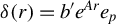
$\delta (r)=b'e^{Ar}e_p$
 , that is,
$v(t)$
 satisfies the continuous-time measurement equation
$v(t)=b'Y(t)$
 , as in (7), and the dynamics of
$Y(t)$
 are governed by the transition equation (6). In this model, the null hypothesis of interest is that
$\alpha _c=0$
 , the stationary alternative being
$\alpha _c<0$
 . Assuming that
$y(t)$
 is skip-sampled, as in (17), the observations satisfy the discrete-time modelFootnote
5

where
$\beta _h=e^{\alpha _c h}$
 . In this example, testing for a zero root can be based on
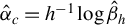
$\hat \alpha _c = h^{-1}\log \hat \beta _h$
 , where
$\hat \beta _h$
 denotes the ordinary least squares estimator of
$\beta _h$
 using (27), and some results in this vein can be found in Chambers (Reference Chambers2015). Noting that
$\log x = (x-1) + O\big ((x-1)^2\big ) (0<x\leq 2)$
 ,Footnote
6
we thus consider the approximation
$\log \hat \beta _h \approx \hat \beta _h-1$
 . We have

Under the null hypothesis (
$\alpha _c=0$
 ), it follows that
$\beta _h=1$
 and so standard arguments lead us to consider

Also under the null hypothesis, the form of
$u_{th}$
 simplifies to

using the notation of Section 3 whose results are relevant here. For example, Theorem 3(c) shows that
$Y_{th}^f$
 can be represented as the sum of a DTLP in
$\xi _{th}$
 plus an additional random disturbance
$\eta _{th}$
 , while Proposition 2 shows that a summability condition of the form (25) applies to the matrix norms in the DTLP component. Furthermore, we find from Theorem 4(b) that

where
$W(r)$
 is a Wiener process and
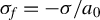
$\sigma _f=-\sigma /a_0$
 . This IP for
$u_{th}$
 leads, via standard manipulations,Footnote
7
to the following asymptotics:

where
$\gamma _{h,0}^f$
 is defined in Theorem 4(c). It then follows that

In order to use this statistic for inference it is, of course, necessary to deal with the nuisance parameters
$\gamma _{h,0}^f$
 and
$\sigma _f^2$
 , and a variety of methods can be used to achieve this, many of which are described in Choi (Reference Choi2015). A similar approach can also be taken in the case of a flow variable.
5. CONCLUDING COMMENTS
In this article, we have considered covariance stationary ARMA processes in continuous time that are sampled at discrete-time intervals and have examined conditions on the continuous-time process such that some of the relevant results of Phillips and Solo (Reference Phillips and Solo1992) can be utilized for normalized sums of the discrete-time observations. The coefficient summability conditions of PS92 are satisfied for the stationary ARMA process although some strengthening of the assumptions regarding the random measure that drives the process is required in order that the discrete-time innovations satisfy the PS92 conditions. The results cover both discretely-sampled stock and flow variables and an illustrative example of their use has been provided. The results could also be extended to the case where the underlying CARMA process is a vector rather than a scalar, a process which is already facilitated by the need to consider a state vector in the proofs here.
Although we have focused on continuous-time counterparts to the PS92 i.i.d.
$\mathcal {A}$
 innovation conditions, it nevertheless would appear possible to extend the results to continuous time versions of their martingale difference sequence conditions (
$\mathcal {B}$
 ) and stable law i.i.d. conditions (
$\mathcal {C}$
 ) when the innovations may have undefined means. Such extensions would be particularly fruitful for CARMA models for financial data where these alternative assumptions are commonly employed.
APPENDIX
This section contains proofs of Theorems 1 and 3 and Propositions 1–3. Owing to space constraints the proofs of Theorems 2 and 4—which are more detailed—can be found in the Supplementary Material along with some additional results which are required in the proofs.
Proof of Theorem 1.
(a) From (13), the form of
$\Theta (r)$
 and
$\tilde \zeta (dt)$
 follows immediately. For the square-integrability condition, we have

Note that

where we have used
$e^{x+iy} + e^{x-iy} = e^x(\cos y + i\sin y) + e^x(\cos y - i\sin y) = 2e^x\cos y$
 and
$|\cos y|\leq 1$
 . It follows that

(b) The form of
$\theta (r)$
 is obvious by noting that
$X(t)=b'Y(t)$
 . For the square-integrability condition, we use the inequality
$\mbox {tr}\{AB\}\leq \|A\|\|B\|$
 , noting that
$\theta (r)=\mbox {tr}\{e^{Ar}e_pb'\}$
 . We find, noting that
$\|e_p\|=1$
 , that

the integral of which is clearly finite in view of (a).
(c) From (14), we can write

from which it follows that

as required owing to the fact that

The covariance matrix
$\Omega _h$
 follows straightforwardly from the definition of
$\epsilon _{th}$
 and it is clear that
$C_{h,0}=I_p$
 . From (9), we can write
$e^{Ahj} = Pe^{\Lambda hj}P^{-1}$
 ; it follows that

The inequality for
$\|C_{h,j}\|$
 then follows. As for the square-summability we have, from (a),

as
$0<e^{-2hr_k}<1$
 .
Proof of Theorem 2. The proof is contained in the Supplementary Material.
Proof of Theorem 3.
(a) From the definition of
$Y^f(th)$
 and the CTLP representation of
$Y(t)$
 in Theorem 1(a), we have

where it follows that
$\Psi (r)$
 is as defined in the theorem. For the square-integrability,

For the first term, we have, from the proof of Theorem 1,

and so we find that

Proceeding in a similar fashion for the second term, we obtain

and hence,

(b) The form of
$\psi (r)$
 follows immediately as
$X^f(th)=b'Y^f(th)$
 whilst further noting that
$\tilde \zeta (dt)=e_p\zeta (dt)$
 . Now
$\psi (r)^2=(\mbox {tr}\{\Psi (r)e_pb'\})^2\leq \|\Psi (r)\|^2\|e_pb'\|^2$
 and so

using part (a).
(c) The most straightforward way to derive the DTLP representation for
$Y_{th}^f$
 is to begin with (6) and to integrate over the interval
$(th-h,th]$
 , yielding

In view of A being nonsingular under Assumption 2, we can solve for the flow to give

But, from Theorem 1(c), we have

Substituting into the expression for
$Y_{th}^f$
 yields

where
$\xi _{th} = A^{-1}\epsilon _{th}$
 ,
$\eta _{th} = -A^{-1}e_p\zeta _{th}$
 ,
$B_{h,0}=I_p$
 , and
$B_{h,j} = C_{h,j}-C_{h,j-1} (j=1,2,\ldots )$
 , as required.
Proof of Theorem 4. The proof is contained in the Supplementary Material.
Proof of Proposition 1.
$\underline {\mathcal {S}_1^c}$
 : Using the inequality for
$\|C_{h,j}\|$
 in Theorem 1(c), we obtain

owing to convergence of the final series which can be verified using, for example, d’Alembert’s ratio test:

for all
$k=1,\ldots ,p_1+p_2$
 .
$\underline {\mathcal {S}_3^c}$
 : Let
$r_m=\min _{1\leq k\leq p_1+p_2}\{r_k\}$
 . Using the inequality in Theorem 1(c), we obtain

the series being convergent as can be verified using d’Alembert’s ratio test, for example.
$\underline {\mathcal {S}_5^c}$
 : This follows from
$\mathcal {S}_1^c$
 :

$\underline {\mathcal {S}_6^c}$
 : Using the inequality for
$\|C_{h,j}\|$
 in Theorem 1(c) once more,

the convergence of which follows because

as required.

SUPPLEMENTARY MATERIAL
The supplementary material for this article can be found at https://doi.org/10.1017/S026646662610070X.
FUNDING STATEMENT
The author declares that no specific funding has been received for this article.
COMPETING INTEREST STATEMENT
The author declares that no competing interests exist.




 Open access

