1. INTRODUCTION
In economics and finance, continuous-time models have been widely used to study the dynamics of underlying state variables, such as asset prices, exchange rates, or spot interest rates. The basic modeling approach in this literature is to assume that the underlying state variables follow a stochastic differential equation.
In the parametric specification of a stochastic differential equation, it is assumed that the functional forms of the drift and diffusion functions are known, apart from a finite number of unknown parameters. Given the parametric specification of a stochastic differential equation, researchers have proposed many different methods to estimate the unknown parameters and to derive the statistical inferences from the discrete observations.
The validity of these estimation and inference procedures, however, is conditional on the hypothesis that the continuous-time model described by a stochastic differential equation is correctly specified. Unfortunately, economic theory typically does not suggest functional forms for the continuous-time model. Model misspecification may lead to misleading conclusions in inference and hypothesis testing. This motivates the development of model specification tests for continuous-time models.
Gallant and Tauchen (1996) proposed a minimum chi-square specification test for continuous-time models using the efficient method of moments. Aït-Sahalia (1996b) proposed a specification test1
Pritsker (1998) uses a Monte Carlo simulation method to examine the specification test of Aït-Sahalia (1996b) and finds that it has a poor finite-sample performance. The main reasons are the highly persistent dependence of the interest rate and the slow convergence of the nonparametric estimator for the density function (Pritsker, 1998, p. 451).
It is noted that the null hypothesis of all the previously mentioned tests is that both the drift and diffusion functions are specified correctly. Under such a null hypothesis, although these tests can detect a wide range of model misspecifications, they cannot reveal possible sources of model misspecifications. However, for the specification analysis of the continuous-time model, when a misspecified model is rejected, one would like to explore the possible reasons for the rejection. Specifically, is the rejection due to the misspecification from the drift function or the diffusion function? When economic theory provides little guidance about the specification of the drift and diffusion functions, it is advantageous to be able to develop a reliable test that can detect whether the model misspecification comes from the drift function or the diffusion function. It should be mentioned that transition-density-based tests can be used to test the specification of the diffusion function (drift function) only through presupposing both the correct specification of the drift function (diffusion function) and the availability of the closed-form expression of the model-implied transition density. Unfortunately, even if the drift function (diffusion function) is specified correctly, the closed-form expression of a transition density still cannot be available for most continuous-time models. In fact, Wong (1964) showed that a stationary diffusion process has a closed-form expression of its transition density only if it has a linear specification for the drift function and a quadratic specification for the diffusion function. As a consequence, these transition-density-based tests are only applicable to very rare continuous-time models.
The limitations of the previously mentioned tests and the recent developments in nonparametric estimation techniques of a continuous-time model prompt us to make use of nonparametric estimation techniques in developing tests for a parametric form of a continuous-time model by directly testing the specifications of its drift and diffusion functions, without relying on the model-implied density function or model-implied moment condition. Corradi and White (1999) provided a first step in this direction. With knowledge of the functional form of the drift function not required, Corradi and White (1999) proposed a specification test for the diffusion function based on discrete sampling observations.
As pointed out by Corradi and White (1999), however, their test can only be used to test a parametric diffusion function at a given point, and the time span of observations is fixed. Thus, their test cannot be used to detect diffusion function misspecifications over a continuous range of the state variable.
Based on discrete observations, we propose a new test of the functional specification of the diffusion function without any restriction on the functional form for the drift function. The test can be used to test the parametric specification of the diffusion function over a time interval that can be fixed or lengthened to infinity. Using theories of degenerate U-statistics, the test statistic is shown to be asymptotically distributed standard normal under the null hypothesis, although diverging to infinity if the parametric specification is misspecified over a significant range. This paper is organized as follows. In Section 2 we state the hypothesis of interest and introduce our test statistic. In Section 3 the asymptotic properties of the test are discussed. The size and power performance of the test are examined by Monte Carlo study in Section 4. Section 5 concludes. The proofs are provided in the Appendix.
2. THE HYPOTHESIS AND TEST STATISTIC
The model we consider is the following autonomous stochastic differential equation:

with initial condition xt0, where xt is the state variable and wt is a standard Brownian motion process. The functions μ(.) and σ2(.) are, respectively, the drift function (the instantaneous conditional mean) and the diffusion function (the instantaneous conditional variance) of the process xt.
We assume that the process xt is observed at {t = t1,t2,…, tn} in the time interval [t0,T]. Although all our results could be derived for nonequispaced data, the only complication being notational, for ease of presentation we will discuss only the equispaced data case. Consequently, we let {xt = xt0+[utri ]n,xt0+2[utri ]n,…, xt0+n[utri ]n} be n equispaced observations on the process xt at dates {t1 = t0 + [utri ]n,t2 = t0 + 2[utri ]n,…, tn = t0 + n[utri ]n}, where [utri ]n = (T − t0)/n is the sampling interval.
We use the notation xn,j to express the observation on the process xt at t = t0 + j[utri ]n, i.e., xn,j ≡ xt0+j[utri ]n, where j = 1,2,…, n.
A parametric family of the specification of the diffusion function σ2(.) is {σ02(x,θ) : θ ∈ Θ}, with Θ being a subset of Rd1 . We want to justify the use of a parametric specification of the diffusion function without knowledge of the functional form of the drift function. Thus, the null hypothesis to be tested is that the parametric specification of σ2(.) is correct:

The alternative hypothesis is σ2(x) ≠ σ02(x,θ) for all θ ∈ Θ over a significant range, i.e.,

Our testing approach is based on the squared error goodness-of-fit function between σ2(.) and σ02(x,θ),

where π(x) and F(x) are, respectively, the unknown density function and cumulative distribution function of xt. Distance measures similar to (4) were used as a basis for testing the model specifications of either a parametric density function or a general regression function by, e.g., Bickel and Rosenblatt (1973), Hall (1984), Fan (1994), Aït-Sahalia, Bickel, and Stoker (2001), and Li and Tkacz (2006).
The introduction of the density function π(x) in (4) is to avoid the problem of trimming the small values of the random denominator in nonparametric estimation of the diffusion function. The inclusion of the weighting function a(x) in (4) allows us to focus goodness-of-fit testing on particular ranges of the state variable. Specifically, we will assume a(x) to be bounded with compact support S ⊂ R (Assumption 8 in Section 3). This assumption will help us to avoid technical problems in proving uniform convergence of the nonparametric estimations of the marginal density and diffusion function on S. By choosing an appropriate a(x), the specification test can be tailored to the empirical question of interest. In practice, a(x) can typically be chosen as the indicator function of a compact set related to the empirical question of interest. For example, to infer the behavior of the short-term interest rate within a range of levels, say, [0.05, 0.10], only the paths of the state variable that cross the interval [0.05, 0.10] are used in the specification analysis.
Under the null hypothesis H0, we have I(θ0,σ02) = 0, and under the alternative H1, we have I(θ,σ02) > 0 for any θ ∈ Θ. Hence, the measure I(θ,σ02) > 0 can be used as an indicator for the misspecification of the diffusion function σ2(.).
If σ2(x),θ0, and π(x) were available, then we could estimate I(θ0,σ02) by its sample analogue

. To get a feasible test statistic, we need to estimate σ2(x),θ0, and π(x).
Under both H0 and H1, the true, unknown σ2(x) can be estimated by the kernel method,2
Downing (1999) and Chapman and Pearson (2000) provide Monte Carlo simulation evidence that contrary to the simulation results of the kernel density estimator by Pritsker (1998), the finite-sample performance of the nonparametric estimator of the diffusion function is very good and notably successful.

where K(.) is a kernel function, and hn is a sequence of bandwidth parameters.
As can be seen from (5), the nonparametric estimator

is built without imposing any restrictions on the functional form of the drift function. The derivation of the asymptotic distribution of the nonparametric estimator

depends crucially on the assumption [utri ]n → 0 as n → 0 (Jiang and Knight, 1997; Bandi and Phillips, 2003). In fact, Nicolau (2003) showed that without the assumption [utri ]n → 0 as n → 0, the nonparametric estimator (5) is not consistent. In contrast, in a semiparametric model with the drift function specified parametrically, the semiparametric diffusion function estimator proposed by Aït-Sahalia (1996a) and Kristensen (2004) required that the sampling interval [utri ]n be fixed to obtain asymptotic results. Because the objective of this paper is to construct a test for the specification of the diffusion function without any functional form specification of the drift function, the nonparametric estimation procedure (5) based on [utri ]n → 0 as n → 0 is used to construct our test statistic. The estimator of

, is defined as follows:

Corradi and White (1999) provided regularity conditions under which

is a quasi-maximum likelihood estimator. These regularity conditions will be given in the assumptions listed in Section 3.
The parametric function σ02(xn,i,θ0) is estimated by

. The unknown density function of xt,π(x), can be consistently estimated by the kernel estimator,
3The drift parameters do not enter our test statistic, and as a result, our test does not suffer the quantitatively significant bias from the estimator of the level of the persistent dependence that the Aït-Sahalia test does (Pritsker, 1998). Indeed, as pointed out by Pritsker (1998), a nonparametric estimator of the density function suffers from the small sample bias. However, the large sample size available (e.g., the high-frequency data) makes it possible to estimate the density function precisely (Hong and Li, 2005; Lavergne and Vuong, 2000; Li, 1999). Even though the nonparametric method has some cost associated with it (i.e., very large samples and an accurate measurement of the function; Pagan and Ullah, 1999), it remains a reliable and powerful tool for analyzing financial data.

Let

be the empirical cumulative distribution estimator of F(x). Inserting the preceding estimates into the definition of I(θ0,σ02), given by (4), yields the following estimator of I(θ0,σ02):

Our test statistic is a properly centered and scaled version of In,

where

3. ASSUMPTIONS AND THE LIMITING DISTRIBUTION OF THE TEST STATISTIC
We specify assumptions for the functions μ(.),σ(.), and the parametric family of {σ02(x,θ) : θ ∈ Θ}, under which the asymptotic validity of this test statistic, Jn, can be established.
Assumption 1. Let D = (l,r) be an open interval with −∞ ≤ l < r ≤ ∞. The functions μ(.) and σ(.) are at least twice continuously differentiable on D.
Assumption 2. σ2(x) > 0 for any x ∈ D.
Assumption 3. The global growth condition is satisfied, i.e., there exists a positive constant, CD, such that for every x,y ∈ D,

Assumption 4. We define S(α) as

where c is a generic fixed number belonging to D. We require S(α) to satisfy limα→l S(α) = −∞, and limα→r S(α) = ∞.
Assumption 5. lim|x|→∞|σ(x)/[2μ(x) − σ(x)σ′(x)]| < ∞, lim|x|→∞ σ(x)π(x) = 0.
Assumption 6. The parametric space, Θ, is compact. For any θ ∈ Θ the given function σ0(x,θ) satisfies Assumptions 1–5. The functions ∂σ02(x,θ)/∂θ,∂2σ02(x,θ)/∂θ∂θ′, ∂σ02(x,θ)/∂x, and ∂2σ02(x,θ)/∂x∂θ exist and are continuous on D × Θ.
Assumption 7. For almost all (x,θ) ∈ D × Θ,σ02(x,θ1) ≠ σ02(x,θ1) if θ1 ≠ θ2. For at least finitely many x, there exists a constant, C1, such that 0 < C1 ≤ σ0(x,θ0) ≤ C1−1. The function Prxt0(σ0(x,θ) > 0) = 1 for (t,θ) ∈ [t0,T] × Θ, where Prxt0 denotes the probability measure generated by the initial value xt0.
Assumption 8. a(x) is a given Borel measurable function and bounded with compact support, S ⊂ D. The function π(x) and its derivative are continuous and bounded on D, and π(x) is bounded away from zero on the compact support, S, of a(x). There exists α > 0, such that ∫ exp(αx2)π(x) dx < ∞.
Assumption 9. K(.) is a bounded and symmetric function about 0, with ∫K(u) du = 1 and ∫|u|K(u) du < ∞, and ∫uK(u) du = 0.
Assumptions 1 and 2 ensure the existence and uniqueness of a strong solution to the stochastic differential equation (1). Assumption 3 is used to establish some important moment inequalities (e.g., Friedman, 1975, Thm. 2.2, p. 127) that are needed to derive asymptotic results. Assumption 4 is used to guarantee that the exit time from D is infinite (Ikeda and Watanabe, 1981, Thm. 3.1, p. 362). Assumption 5 is from Hansen and Scheinkman (1995, p. 801). Aït-Sahalia (1996a, p. 552) proved that under Assumption 5 the various classical mixing properties of the discrete observations from the stochastic differential equation (1) are satisfied. In particular, the observation process is absolutely regular with geometric decay rate. Without this assumption, the central limit theorem (CLT) for second-order degenerate U-statistics of absolutely regular processes can fail. Assumptions 6 and 7 were used by Corradi and White (1999, Thm. 3.2, p. 261) to ensure that

, where θ* ∈ Θ and θ* = θ0 under the null hypothesis. Assumption 8 requires a(x) to be bounded with compact support. As we mentioned earlier, without this assumption, we can not prove uniform convergence of the nonparametric estimations of the marginal density and diffusion function on S. In practice, S can typically be taken as the indicator function of a compact set related to the empirical question of interest. Assumption 9 is a standard regularity condition imposed on a kernel function.
The asymptotic null distribution and consistency of Jn are provided in the following theorem.
THEOREM 1. Suppose Assumptions 1–9 hold and hn = O(n−1/γ), where 1.5 < γ < 4.5. If T is either fixed or T → ∞,Thn1/2 → 0, and [utri ]n → 0 as n → 0, then
(i) under H0,Jn → N(0,1) in distribution as n → ∞, and

is a consistent estimator of v2, where v2 = 8 ∫σ8(x)π4(x)a2(x) dx ∫[∫K(u)K(w + u) du]2 dw;
(ii) under H1,Pr(Jn ≥ Bn) → 1, for any nonstochastic sequence Bn = o(nhn1/2).
Proof. See the Appendix.
4. MONTE CARLO SIMULATION
In this section, we examine the finite-sample performance of the test using Monte Carlo simulations. As stated in Section 1, assuming that the drift function is specified correctly and that the closed-form expression of the model-implied transition density is available, transition-density-based tests can also be used for the specification of the diffusion function in a diffusion process. Hong and Li (2005) conducted a simulation study to examine the size and power of their tests. For comparison, we adopt simulation designs that are similar to those of Hong and Li (2005). To examine the test's size performance, we simulate data from the Vasicek (1977), Cox, Ingersoll, and Ross (1985) (CIR hereafter), and drift-misspecified CIR (DMCIR hereafter) models, respectively.
The Vasicek model is

The CIR model is

The DMCIR model is

For Vasicek's model, the null hypothesis is that the diffusion function is a constant; i.e., H0 : σ2(x) = constant. Under the null hypothesis, the estimator of θ = σ2 is given by

. Under the assumption that the drift function is correctly specified as β(α − x), the Hong and Li (2005) test can be used to test the null hypothesis by testing whether the data are generated from a normal transition density (Hong and Li, 2005, p. 48). In the Vasicek model, the parameter β determines the persistence of the process. The smaller β is, the higher the level of persistence in the process, and, consequently, the slower the convergence to the long-run mean, α.
As with Hong and Li (2005) and Pritsker (1998), to examine the impact of the level of persistence on the size performance of our test, we consider both low and high levels of persistent dependence and adopt their parameter values. The parameter values for low and high levels of persistent dependence are, respectively, (β,α,σ2) = (0.85837, 0.089102, 0.002185) and (β,α,σ2) = (0.214592, 0.089102, 0.000546).
To examine the test's size performance when the drift function is misspecified, we consider two cases. For case 1, the data are assumed to be from the CIR model, but they are generated from the DMCIR model. For case 2, the data are assumed to be from the DMCIR model, but they are generated from the CIR model. For both cases, we test the null hypothesis that the diffusion function is σ2x; i.e., H0 : σ2(x) = σ2x. Obviously, in both the CIR model and the DMCIR model, with the drift functions being misspecified, the diffusion functions are correctly specified. The parameter values of the CIR model are taken as (β,α,σ2) = (0.89218, 0.090495, 0.032742), which are from Hong and Li (2005), whereas the parameter values of the DMCIR model are taken as (α−1,α0,α1,α2,σ2) = (0.00107, −0.0517, 0.877, −4.604, 0.032742). Under the null hypothesis, the estimator of the parameter, θ = σ2, is given by

.
Because the Vasicek and CIR models have closed-form transition density and marginal density functions (Pritsker, 1998, p. 456; Hong and Li, 2005, p. 49), the simulated sample path can be constructed by their transition densities. The initial values are drawn from their marginal densities. The discrete observations of sample size n are generated over a time period [0,T] with a sampling interval of [utri ]n = T/n. For the DMCIR model (15), because its transition density has no closed form, data are simulated using Milstein's scheme (see (19) in this section). Throughout the experiment, we generate 500 realizations of a random sample {xn,j}j=1n for sample sizes n = 250, 500, 1,000, 2,500, respectively. We discard the first 500 observations to eliminate any start-up effects. T is set to 1 and 5 to consider the impact of the sample interval on the test performance.
To study the test's power performance, we consider two cases. For case 1, the null hypothesis stipulates that the data are generated by a model with a constant diffusion function; i.e., H0 : σ2(x) = constant. However, we simulate data from three different models: the CIR model, the Chan, Karolyi, Longstaff, and Sanders (1992) (CKLS hereafter) model, and the Aït-Sahalia (1996b) nonlinear drift model. The same parameter values in Hong and Li (2005) are again adopted. If we impose the assumption that the drift function is correctly specified as β(α − x), the Hong and Li (2005) test can be used to test the null hypothesis by testing whether the data are from a normal transition density.
The CKLS model is

with parameter values (β, α, σ2, ρ) = (0.0808, 0.0972, 0.52186, 1.46).
The Aït-Sahalia (1996b) nonlinear drift model is

with parameter values (α−1,α0,α1,α2,σ2,ρ) = (0.00107, −0517, 0.877,−4.604, 0.64754, 1.50).
For case 2, the null hypothesis stipulates that the data are generated by a model with the diffusion function σ2x. However, the data are simulated from three different models: the CKLS model (16), the nonlinear drift model (17), and a modified CKLS (MCKLS) model.
The MCKLS model is

with the parameter values (β,α,σ2) = (0.89218, 0.090495, 0.032742) used in the CIR model. Note that the process (18) has a nonlinear diffusion function and the same drift function as in the CIR model. Particularly, the linear diffusion function in the CIR model is tangential to the diffusion function in the MCKLS model at point 0.090495. This design helps in evaluating the test's power for testing curvature. For the CKLS model (16), the Aït-Sahalia (1996b) nonlinear drift model (17), and the MCKLS model (18), because their transition densities have no closed forms, we simulate data using Milstein's scheme,

where εt is a standard normal distribution. The initial value is set to equal the average interest rate level of the data set in Aït-Sahalia (1996b).
Throughout this experiment, we use the standard normal kernel. The bandwidth parameter hn is chosen according to hn = cσx n−1/γ, where σx is the standard deviation of observations. We choose γ = 2.1,3.5. The choice of hn satisfies the conditions of Theorem 1. To check the sensitivity of the test with respect to the choice of bandwidth hn, we change hn through different values of c: c = 0.5, 1, 1.5. The function a(x) is the indicator function of the interval S = {x|x ∈ [0.002, 2]}. The critical value zα is from the standard normal distribution; i.e., z0.01 = 2.33,z0.05 = 1.645, and z0.1 = 1.28.
Table 1 reports the estimated size of the test. Four general conclusions can be drawn from the table. First, the test has satisfactory size performance at all three levels for sample sizes as small as n = 250. In contrast, it is clear that, under the same simulation setting, the Hong and Li tests show strong overrejections under the 1% level (Hong and Li, 2005, Figs. 1 and 2), and the size of their tests is about 2.1% on average, even if the sample size increases to 5,500. Second, the impact of the level of the persistent dependence on the size of the test is minimal, which suggests that the test achieves robustness to the persistent dependence. This result can be explained by the fact that the test statistic is independent of the specification of the drift function, which determines the level of the persistent dependence. Third, the test still exhibits a satisfactory size performance even if the drift function is misspecified. In contrast, the Monte Carlo simulation shows that, under the null hypothesis that the data are generated from the CIR model, the power of the Hong and Li (2005) tests for rejecting the DMCIR model is about 59%, even if the sample size is increased to 2,500 across lag orders from 1 to 20. In other words, the Hong and Li (2005) tests strongly reject the correct null hypothesis of σ2(x) = σ2x. It is obvious that the rejection arises because of the misspecification of the transition density. Fourth, note that the estimated size of the test is quite stable over different choices of bandwidth, particularly for large samples.
Percentage of rejections of the true H0

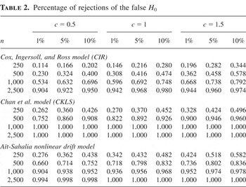
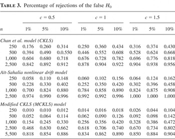
Table 2 reports the estimated power of the test when the null hypothesis is that the diffusion function is a constant but in fact the data are generated from the CIR model, the CKLS model, and the Aït-Sahalia (1996b) nonlinear drift model, respectively. Table 3 reports the estimated power of the test when the null hypothesis is that the diffusion function is σ2x but in fact the data are generated from the CKLS model, the Aït-Sahalia (1996b) nonlinear drift model, and the MCKLS model, respectively.
Percentage of rejections of the false H0

Percentage of rejections of the false H0

The simulation results of the test's power performance lead to three conclusions. First, Tables 2 and 3 indicate that the test detects the misspecifications of the diffusion functions quite well in both the Vasicek and CIR models against their respective alternatives. For a given alternative, the test's power always increases rapidly with respect to the sample size, in line with the test's consistency property. By comparison, the power of the Hong and Li (2005) tests in detecting the Vasicek model against the CIR model is about 50% when n increases to 2,500, which is noticeably worse than against the CKLS model and the Aït-Sahalia (1996b) nonlinear drift model (Hong and Li, 2005, Fig. 3). However, under the same simulation setting, the power of the test is above 90%. Second, the test has good power in detecting the CIR model against the MCKLS model when the sample size increases to 2,500. This test, however, has a lower power in detecting the CIR model against the MCKLS model than the CKLS model and the Aït-Sahalia (1996b) nonlinear drift model. This result can be explained by the fact that the diffusion function in the MCKLS model is closer to the diffusion function in the CIR model than in the two other models. Third, even though the test's power is already quite stable over different choices of hn for large samples (n = 1,000,n = 2,500), the higher the value of the bandwidth, hn (i.e., the higher the value of c), the higher the test's power. This result can be explained by the fact that the test statistic diverges to +∞ at the rate of nhn1/2 under the alternative. Hence, a higher hn (in a certain range) will lead to a more powerful test against some fixed alternatives (in finite samples). This result does not mean that one should use a very large value of hn in practice, because it would oversmooth the data and hence obliterate any deviation of the data from the null data-generating process. Of course, one should not use a very small value of hn, because it could result in an inaccurate kernel estimation. Specifically, an hn that is too small tends to make the test less powerful. Because the test is based on high-frequency data, the large sample sizes available should make the choice of hn less crucial than the moderate sample size. How to choose the bandwidth optimally, so that the test's power is maximized and the size is kept under control, is left for future research.
Simulation results for T = 5 are not presented but are available from the author. They are qualitatively similar to those for T = 1.
5. CONCLUSION
In this paper, we propose a consistent test for the parametric specification of the diffusion function in a diffusion process without any restrictions on the functional form of the drift function. The test is based on a comparison of the kernel estimate of the true unknown diffusion function with the parametric specification of the diffusion function. It is shown to have the standard normal distribution under the null hypothesis. The Monte Carlo simulation results suggest that the overall performance of the test is satisfactory.
Extensions to multidimensional diffusion processes (including unobservable state variables) and applications to evaluate the performance of a variety of specifications for the diffusion function in the spot interest rate process (Durham, 2003) will be considered for future work. It would also be useful to develop a test for the parametric specification of the drift function in a diffusion process.
APPENDIX: Proofs
Let {Xn,l} ≡ {Xn,l, : l ≤ n; n ≥ 1} be a triangle array of random variables and Ms,tn denote the sigma algebra generated by (Xn,s,…, Xn,t) for s ≤ t.
DEFINITION.
(i) {Xn,l} is said to be a strictly stationary triangular array of random variables if for positive integers s1, s2, and k, {Xn,s1,Xn,s1+1,…, Xn,s1+k} and {Xn,s2,Xn,s2+1,…, Xn,s2+k} have the same joint distribution, where s1 + k ≤ n,s2 + k ≤ n.
(ii) Let {Xn,l} be a strictly stationary triangular array of random variables and βn,τ = sups+τ≤n E[supA∈Ms+τ,n{P(A|M1,sn(n)) − P(A)}]. Then, {Xn,l} is said to satisfy an absolute regularity condition with the mixing coefficient βn,τ if βn,τ → 0 as τ → ∞.
LEMMA 1. Let ξn,1,…, ξn,n be random vectors taking values in Rd2 satisfying an absolute regularity condition with the mixing coefficient βn,τ. Let a(y1,…, yk) be a Borel measurable function such that, for some δ > 0,

exists. Then,

where

and m = ij+1 − ij,Fni1,…, ij(zi1,…, zij) is the distribution function of random vectors ξn,i1,…, ξn,ij and i1 < i2 < ··· < ij.
Proof. Lemma 1 follows straightforwardly from Lemma 1 in Yoshihara (1976). █
For notational simplicity, hn and K((xn,j − x)/hn) are expressed by h and Kj(x), respectively. We use Ej to express the conditional expectation with respect to the σ-field generated by {xu : u ≤ t0 + j[utri ]n}. The symbol C denotes a generic big enough positive constant. The notation A ∼ B means that A has an order no larger than that of B. Also let B(.,.,.) be a Borel measurable function and Fn(x,x) be the joint distribution function for (xn,i,xn,j), where i ≠ j. We denote Ei [B(xn,i,xn,j,xn,k)] ≡ ∫B(x,xn,j,xn,k) dF(x), Ek [B(xn,i,xn,j,xn,k)] ≡ ∫B(xn,i,xn,j,x) dF(x), and Ei,j [B(xn,i,xn,j,xn,k)] ≡ ∫B(x,x,xn,k) dFn(x,x).
LEMMA 2. Suppose that Assumptions 1–4 and 6 hold, E(x2d) < ∞ for some positive integer d, and t′ ∈ [t0,T). Then,
(i) for t′ > t0 + j[utri ]n:

where Dn = 22(2d−1)CD2d{(t′ − t0 − j[utri ]n)d + [d(2d − 1)]d}.
(ii) Let

, where zn,j = (xn,j,xn,j+1). Then, under the null hypothesis, for x ∈ S:

and

where ξ > 1.
Proof of (i) of Lemma 2. (A.1) directly follows Theorem 2.2 of Friedman (1975), simply by replacing the unconditional expectation by conditional expectation. █
Proof of (ii) of Lemma 2. For notational simplicity, we denote

by ∫[utri ]n g(u) du, where g(u) is any integrable function. An application of Itô's formula yields

We will prove (ii) of Lemma 2 by showing An1 = O([utri ]n1/2n−1),An2 = O(n−1h), and An3 = O(n−3/2h1/ξ−1). From Assumptions 3 and 4, (A.1), and Schwarz's inequality, it is straightforward to have that An1 = O([utri ]n1/2n−1). For An2, by Assumption 4 we have

For An3, under H0, from Assumption 6 and Hölder's inequality, there exists ξ > 1 such that

where η = (1 − ξ−1)−1. Hence (A.2) holds. We show (A.3).

where

.
Using (i) of Lemma 2, the mean value theorem (to

),

, and changing the variable by (xn,j − x)/h = u, it is straightforward to have An32 = O((n3h)−1) and An33 = O([utri ]n1/2(n5/2h)−1) + O(n−5/2). We next consider An31.
Applying Itô's formula to (xn,j+1 − xn,j)4 and (xn,j+1 − xn,j)2, we have

By using (i) of Lemma 2, it can be shown that An311 = O([utri ]n1/2(n2h)−1),An312 = O([utri ]n1/2(n2h)−1), An313 = O([utri ]n1/2(n2h)−1 + n−2),An314 = O([utri ]n1/2(n2h)−1),An315 = O([utri ]n1/2(n2h)−1 + n−2), An316 = O([utri ]n1/2(n2h)−1 + n−2), and

Summarizing the preceding discussion, we have shown that

These results imply that (A.3) holds. █
LEMMA 3. Under Assumptions 1–9 and the null hypothesis, In can be written as

where

.
Lemma 3 indicates that the only difference between In and In is that the latter is average over the empirical conditional distribution function instead of F. Lemma 3 shows that this difference is inconsequential for the asymptotic distribution of the test statistic.
Proof of Lemma 3. We need to prove that

First, under Assumption 5 the observed data sequence {xn,t} is absolutely regular with geometric decay rate; i.e., {xn,t} satisfies the absolutely regular condition with mixing coefficient βn,m = O(λm) (Aït-Sahalia, 1996a, p. 552), where λ is a positive constant determined by the integral operator of the diffusion process (1). Let m = [b log n] and κ = log λ where b is a sufficiently large positive constant. Then we have βn,m = O(λm) = O(λ−bκlogλ n) = O(n−bκ).
Recalling

, εn can be written as follows:

We shall show that εni = op((nh1/2)−1) for i = 1,2,3. We will first show that εn1 = op((nh1/2)−1). We define Wi,j,k(xn,k) as follows:

then,

To prove εn1 = op((nh1/2)−1), we need to prove that εn1i = op((nh1/2)−1) for i = 1,2,3. For εn11, because of (xn,i+1 − xn,i)2d = Op([utri ]nd) for d = 1,2 by (A.1) in Lemma 2, we immediately obtain

For εn12, we denote (εn12)2 as

where (εn112)2,(εn122)2, and (εn132)2, respectively, denote the cases where the summation indices satisfy min{|k − k′|,|k − i|,|k − i′|} > m + 1, either i = i′,k = k′ or i = k′, k = i′ and all remaining cases. For (εn112)2, using Ek(Wi,i,k(xn,k)) = 0 and Lemma 1, we have

For (εn122)2,

For (εn132)2, using the Hölder inequality, we have

From (A.9)–(A.11), we have

To evaluate εn13, we consider the second moment of (nh1/2εn13)2,

We consider four different cases: (a) for any two summation indices l and L from k,i,j,k′,i′,j′,|l − L| > m + 1 for all L ≠ l; (b) there exist exactly four different summation indices such that for any index l from these four indices, |l − L| > m + 1 for all L ≠ l; (c) there exist exactly three different summation indices such that for any index l from these three indices, |l − L| > m + 1 for all L ≠ l; and (d) all the other remaining cases. We will use EAs to denote these cases (s = a, b, c, d). For case (a), using EkWi,j,k = 0 or Ek′Wi′,j′,k′ = 0 and Lemma 1, we have

For case (b), we only need to consider the case |k − k′| ≤ m + 1, because otherwise we will have k or k′ is at least m periods away from any other indices and by Lemma 1, we know it is bounded by Cn6βn,m1/2 = o(1). With |k − k′| ≤ m + 1, we must have at least m + 1 periods away from any other indices for l = i,j,i′,j′. Hence, repeating the application of Lemma 1 yields

For case (c), we only need to consider |k − k′| ≤ m + 1, |k − l| ≤ m + 1 for exactly one l ∈ {i,j,i′,j′}, because otherwise it will be bounded by Cn6βn,m1/2 by Lemma 1. By symmetry we only need to consider l = i. Repeating the application of Lemma 1 yields

For case (d), for any three different l's, |k − l| ≤ m + 1 for all k ≠ l; case (d) has at most m3n3 terms. Hence, using Lemma 1, we have

From (A.13)–(A.17), we have

Finally, from (A.8), (A.12), and (A.18), εn1 = op((nh1/2)−1).
To prove εn2 = op((nh1/2)−1), expanding

around θ0 yields

Using (A.19), εn2 can be expressed as

Using the same approach as we used to prove that εn1 = op((nh1/2)−1), we can prove that εn21 = op((nh1/2)−1). By (xn,i+1 − xn,i)2 = Op([utri ]n) and Assumption 5, it follows that εn22 = Op(1). Hence, εn2 = op((nh1/2)−1).
Finally, for εn3, we have

It is easy to show that εn31 = Op(n−2h−1) = op(1) and εn32 = Op(n−1h−1) = op(1). Hence, εn3 = op(nh1/2). █
We will need a CLT for degenerate U-statistics of the triangular arrays of random variables {Xn,l,l ≤ n; n ≥ 1}, which is used in deriving the asymptotic distribution of the test statistic proposed in this paper. We write

where Hn(.,.) depends on n and satisfies ∫Hn(x,y) dFn(x) = 0 for all y and Fn(.) is the marginal distribution function of Xn,t. For every n, let

be an independent identically distributed (i.i.d.) sequence having the same marginal distribution as {xn,l}. Following the same approach as in Fan and Li (1999), we define

. In Lemma 4, which follows, Assumptions (A1)–(A3) in Fan and Li (1999) are said to be satisfied by {Xn,t} if the conditions in Assumptions (A1)–(A3) in Fan and Li (1999) calculated by every row of {Xn,t} are satisfied.
LEMMA 4. Let {Xn,t} be strictly stationary and satisfy the absolutely regular condition with mixing coefficient βn,m. If Assumptions (A1)–(A3) in Fan and Li (1999) are satisfied by {Xn,t}, then we have

in distribution as n → 0.
Proof of Lemma 4. The proof follows in the same way as the proof of Theorem 2.1 in Fan and Li (1999) and thus is omitted here.
Proof of part (i) of Theorem 1. From Lemma 3, we will complete the proof of part (i) of Theorem 1 by showing
(a)

in distribution as n → ∞.
(b)

in probability as n → ∞.
Proof of (a). In can be rewritten as

Let rn(zn,j,x,θ) = rn(zn,j,x,θ) − Ern(zn,j,x,θ), where zn,j = (xn,j,xn,j+1). We decompose In according to

We will show under our assumptions that In1 is asymptotically normal in distribution and In3 and In4 are asymptotically negligible in probability, whereas In2 gives a bias term. First, we prove that nh1/2(In2 − EIn2) → 0 in probability under the null hypothesis.

Changing variable by (xn,j − x)/h = u and using (i) of Lemma 2, we have

For In22, we consider two different cases: (a) min{| j − k| > m + 1} and (b) min{| j − k| ≤ m + 1}. We will use EBa and EBb to denote cases (a) and (b), respectively. By Schwarz's inequality and (A.24), we have

Hence, by Lemma 1, we have


By (A.3), (A.25)–(A.27), and Chebyshev's inequality, it follows that

which characterizes the asymptotic bias term in our test statistic. Using Theorem 3.3.2 and Remarks 3.3.4 and 3.3.5 in Györfi, Härdle, Sarda, and Vieu (1989, Sect. III.3), one can establish the following results:


The proofs of (A.29) and (A.30) are available from the author upon request. By the CLT it is easy to verify that

From (A.28)–(A.31), we obtain the sample analogue of (A.28),

To prove nh1/2In3 = op(1), we evaluate E(nh1/2In3)2. Using Lemma 2 and choosing

in (A.2), we have

From E(In3) = 0, (A.33), and Chebyshev's inequality, it follows that nh1/2In3 = op(1). For In4, choosing

from (A.2) we have

Next, we express In1 in U-statistic form as

Using the Hölder inequality, we have In12 = op((nh1/2)−1) and In13 = op((nh1/2)−1). We will use Lemma 4 to prove that In11 is asymptotically normal in distribution. We now verify that Assumptions (A1)–(A3) in Fan and Li (1999) are satisfied under Assumptions 1–9.
Let H(zn,j,zn,k) ≡ ∫rn(zn,j,x,θ0)rn(zn,k,x,θ0)a(x) dF(x) and

be an i.i.d. sequence having the same marginal distribution as {zn,j}j=1n. Then we have

To evaluate σn2, we first evaluate

.

Applying Itô's formula to (xn,2 − xn,1)2 and (xn,2 − xn,1)4, and using similar arguments as in the proof of Lemma 2, we obtain

and

From (A.36) and (A.37), it follows that

. Hence, we get

To conserve space, the detailed proof of the rest of the conditions of the CLT in Lemma 4 is not incorporated here, but it is available in Li (2005) or from the author.


where

and ζ is slightly larger than 2.


where

.

where

.

where 1 < η < 2. Summarizing the preceding discussion, we have shown that σn2 = O(n−4h−1),μn4 = O(n−8h−3),γn ≡ max{γn11,γn22,γn14} = O(n−4h4/η−4), and vn ≡ max{γn22,γn13} = O(n−8h4/η−6). These results, together with the assumption h = O(n−1/γ) and 1.5 < γ < 4.5, imply (A1)(i)–(iii) in Fan and Li (1999).
Define Gn(zt,zs) ≡ E [H(zn,1,zt)H(zn,1,zs)]. Then,

where

.

where

.

where

. Thus, (A2)(i)–(iii) in Fan and Li (1999) are satisfied.
Finally it is easy to show that Mn in Fan and Li (1999) is bounded by some positive constant. From βn,m = O(n−bκ), we have m2n2βn,m1/2/σn4 = o(1), provided we choose b sufficiently large. Thus (A3)(i) and (ii) in Fan and Li (1999) are satisfied. █
Proof of (b). From Assumption 8, (A.29), and (A.30), we have


From (A.48) and (A.49) it follows that

which implies

by the law of large numbers. Thus, vn2 = v2 + op(1). █ █
Proof of part (ii) of Theorem 1. Given Assumptions 1–9, from Theorem 3.2 in Corradi and White (1999),

is an

-consistent estimator of some θ* ∈ Θ. We can show by using similar arguments as those in the proof of part (i) of Theorem 1 that, under H1,

where ∫[(σ2(x) − σ02(x,θ*))π(x)]2a(x) dF(x) > 0 and vn2 → v2 in probability. Hence, we have Jn = Op(nh1/2). █