1 INTRODUCTION
Empirical research in economics often begins by positing a model which relates quantities of economic interest to the distribution of observable data. Researchers then use model-implied relationships, together with observed data, to construct estimates or bounds for parameters of interest.
Unfortunately, commonly used models impose assumptions which are difficult to validate, and which are sometimes rejected outright. For instance, some models impose functional form restrictions such as linearity, or distributional restrictions on latent error terms. Others impose homogeneity across economic agents, or behavioral assumptions such as utility or profit maximization. Finally, methods that aim to uncover causal or structural relationships impose assumptions regarding unconfoundedness of treatment and the scope for spillovers across units. When we have reason to doubt these assumptions, it can be unclear how to interpret model-implied estimates or bounds. Indeed, absent some restriction on model misspecification, the quantities of interest are necessarily unidentified, and we can learn nothing from data. As would be expected, conventional approaches for inference on the quantities of economic interest are thus invalid under misspecification (see, for instance, Newey, Reference Newey1985; Bugni, Canay, and Guggenberger, Reference Bugni, Canay and Guggenberger2012; Guggenberger, Reference Guggenberger2012a, Reference Guggenberger2012b; Guggenberger and Kumar, Reference Guggenberger and Kumar2012).
An influential econometrics literature, including White (Reference White1982), Hall and Inoue (Reference Hall and Inoue2003), Schennach (Reference Schennach2007), Müller (Reference Müller2013), Hansen and Lee (Reference Hansen and Lee2021), Andrews and Kwon (Reference Andrews and Kwon2024), and Kleibergen and Zhan (Reference Kleibergen and Zhan2025), avoids the inferential problems posed by model misspecification by shifting the focus to “pseudo-true” parameter values, defined as the minimizers of a population objective function. Under mild conditions, these papers show consistency of estimates for the pseudo-true value (in point-identified settings) or the pseudo-true identified set (in set-identified ones). Moreover, these papers provide inference results, for example, showing asymptotic normality of point estimates and deriving consistent standard errors for the pseudo-true value. Some of these results have been highly influential for empirical practice with, for instance, the “sandwich” standard error formula discussed by White (Reference White1982) now widely adopted in the context of maximum likelihood estimation.
While focusing on pseudo-true values allows us to provide statistical guarantees, it leaves open the question of how, if at all, these pseudo-true values relate to the original quantities of economic interest. The literature studying inference on pseudo-true values discusses this tension, with White (Reference White1982) writing “[the estimator] converges to a well defined limit, and may or may not be consistent for particular parameters of interest.” Similarly, Müller (Reference Müller2013) writes that “[it] is important to keep in mind that the pseudo-true parameter of the misspecified model must remain the object of interest for
$\ldots $
 inference to make sense” and Hansen and Lee (Reference Hansen and Lee2021) write that “it is difficult to give economic interpretation to pseudo-true parameter values. Consequently, this limits interest in valid inference procedures for pseudo-true values.”
This article revisits the distinction between true and pseudo-true parameter values. To abstract from sampling uncertainty, we consider a population minimum-distance problem in which the distribution of the data is perfectly observed. We adopt a decision-theoretic, and specifically Bayesian, perspective to ask under what conditions the posterior distribution for
$\theta $
 , given the distribution of the observable data, concentrates around the pseudo-true parameter. Such concentration implies, under mild conditions, that Bayes decision rules converge to plug-in rules based on pseudo-true values.
We provide three main results. First, we characterize a class of joint priors for the data distribution and the quantity of interest
$\theta $
 such that the posterior density for
$\theta $
 is proportional to a transformation of the minimum distance objective function. This proportionality implies that the minimum distance objective is sufficient for decision-making, and hence an optimal way to summarize the data. This is a natural class of priors to consider in the context of minimum distance estimation, since it corresponds to a belief that the minimum distance objective captures all decision-relevant information. We show, under independence and conditional mean-zero restrictions on an implied prior for model misspecification, that proportionality holds if and only if the implicit misspecification prior satisfies a rotation-invariance condition.
Second, we characterize prior sequences in this rotation-invariant class such that the posterior distribution concentrates around the pseudo-true value. These priors assume that the degree of misspecification is negligible, which seems implausible in many economic applications. We further find that concentration is fragile, in the sense that seemingly small changes to the prior lead posterior concentration to fail dramatically.Footnote
1
When posterior concentration fails, researchers with different priors on the form and degree of misspecification will have different posteriors for
$\theta .$

This naturally raises the question of whether it is possible to give positive results under the class of priors we consider. Our third main result constructs confidence intervals that guarantee correct coverage of
$\theta $
 under all priors satisfying our rotation-invariance condition. Since we consider the population problem, there is no randomness due to sampling and we instead define coverage using the ex-ante probability under the prior. Our misspecification-robust confidence intervals:
-
1. are centered at the pseudo-true parameter value,
-
2. require no researcher input beyond the choice of weighting matrix,
-
3. have width proportional to the square root of a population J-statistic, and
-
4. impose no ex-ante upper bound on the degree of misspecification.
Since these intervals are valid under a class of priors motivated by the minimum distance objective, they are a natural option for summarizing misspecification-driven uncertainty in settings where researchers adopt a minimum distance approach.
Inference under model misspecification is closely related to the large literature on partial identification, and the practice of plugging in pseudo-true parameter estimates for decision-making is an instance of what Manski (Reference Manski2021) terms “as-if optimization.” In settings where we are concerned with model misspecification, an alternative approach is to explicitly bound the possible degree of misspecification and derive results which are valid under all data-generating processes satisfying this bound, for instance, by characterizing the identified set for the quantity of interest. We show, however, that computing identified sets under a bound on the norm of the moments at the true parameter leads to counter-intuitive behavior in our setting, where the identified set narrows as the observed violation of the model’s overidentifying restrictions grows worse, rather than widening, as our confidence intervals do.
The next section introduces our population minimum distance setting and formally defines model misspecification and pseudo-true values. Section 3 introduces the decision problem we study and provides our first main result, characterizing the class of priors such that the posterior for
$\theta $
 depends on the data through the minimum distance objective. Section 4 characterizes sequences of priors in this class such that the posterior concentrates on the pseudo-true value and shows that this concentration is fragile in important respects. Finally, motivated by an invariance property derived in Section 3, Section 5 derives our suggested confidence intervals, compares them to identified sets based on bounds for the magnitude of misspecification, and considers several extensions to cases with sampling uncertainty.
2 Setting
2.1 Minimum Distance Model
Suppose that for a set
$\mathcal {D}$
 and
$\Delta (\mathcal {D})$
 the set of distributions on
$\mathcal {D},$
 a researcher observes a distribution
$P\in \mathcal {P}\subseteq \Delta (\mathcal {D}).$
 This corresponds to the large-sample limit of a setting where the researcher observes a sample of n observations
$D_{i}\in \mathcal {D}$
 drawn iid from
$P,$
 since, as
$n\to \infty ,$
 they can consistently estimate P from
$\{D_i\}_{i=1}^n.$
 Though we abstract from it here, we consider a setting with sampling uncertainty in Section 5.Footnote
2
Further suppose that the researcher is interested in an economic quantity
$\theta \in \mathbb {R}^p$
 and has a model that implies that the true
$(\theta ,P)$
 pair satisfies

for known functions
$Y:\mathcal {P}\to \mathbb {R}^{k}$
 and
$X:\mathcal {P}\to \mathbb {R}^{k\times p}.$
 We assume that
$X(P)$
 has full column rank and, unless otherwise noted, assume that the model is over-identified, with
$k>p$
 . We loosely refer to
$g\left (\theta ;P\right )$
 as “moments,” though the linear minimum-distance setting we consider is more general than linear GMM. We focus on linear-in-parameters moments of the form (1) for simplicity, but our exact results for this linear setting will translate to approximate results for models which can be linearly approximated, for instance, under local misspecification as studied by Armstrong and Kolesár (Reference Armstrong and Kolesár2021). We return to this connection in Section 5.
Example: Linear IV
As a first example, suppose that
$D_{i}=\left (Y_{i},X_{i},Z_{i}\right )$
 for
$Y_{i}\in \mathbb {R}$
 a scalar outcome,
$X_{i}\in \{0,1\}$
 a binary endogenous treatment, and
$Z_{i}\in \mathbb {R}^{k}$
 a vector of k mean-zero exogenous variables,
$E[Z_i]=0$
 . We assume that these data are generated from a potential outcomes model, where the potential outcomes
$Y_i(x,z)$
 may in general depend on both
$X_i$
 and
$Z_i,$
 and the potential treatments
$X_i(z)$
 may depend on
$Z_i.$
 The parameter of interest
$\theta \in \mathbb {R}$
 is the average treatment effect (ATE):

which captures the average effect on
$Y_i$
 from changing
$X_i$
 from zero to one.
If the researcher wants to estimate a constant-effect linear instrumental variables model with excluded instrument
$Z_i$
 , this can be justified by assuming that
$Z_i$
 is excluded from
$Y_i, Y_i(x,z)=Y_i(x,z')$
 for all
$(x,z,z')$
 (so one may denote the potential outcome as
$Y_i(x)$
 ), that the instrument is randomly assigned
$Z_i\perp \!\!\!\!\perp Y_i(\cdot ),X_i(\cdot ),$
 and that treatment effects are constant,
$Y_i(1)-Y_i(0)=\theta $
 for all i. Under these assumptions,
$Y_i$
 follows the linear model
$ Y_{i}=X_{i}\theta +\varepsilon _{i},$
 where
$\varepsilon _i=Y_i(0)$
 and
$E\left [Z_{i}\varepsilon _{i}\right ]=0$
 . Consequently,
$\theta $
 solves the moment condition (1) for

which are (up to pre-multiplication by
$E_P[Z_iZ_i']^{-1}$
 ) equal to the reduced-form and first-stage coefficient vectors in the linear IV model, respectively.
$\triangle $

Example: Logit Model
As a second example, suppose that
$D_i = (Y_i, X_i)$
 for
$Y_i \in \{0, 1\}$
 a binary outcome and
$X_i = (1, \tilde {X}_{i})\in \mathbb {R}^2$
 an exogenous variable, where
$\tilde {X}_{i} \in \{x_1, \ldots , x_J\}$
 . If the researcher assumes a logistic regression (i.e., logit) model for
$Y_i,$


where
$\varepsilon _i \sim \textrm {Logistic}(0,1)$
 is independent of
$X_i$
 and
$\psi $
 is a conformable vector of coefficients, then, under this model,

for
$\Psi (u)=\frac {e^u}{1+e^u}$
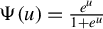 the logistic function or, equivalently,

for
$\Psi ^{-1}(u)=\log \left (\frac {u}{1-u}\right )$
 the logit function.
We suppose that the object of interest
$\theta \in \mathbb {R}^2$
 parameterizes the conditional mean of Y given two distinct as-yet-unobserved values of
${X}_{i}:$


where
$x_1^*,x_2^*\not \in \{x_1, \ldots , x_J\}.$
 The model implies that
$\theta $
 solves (1) for

2.2 Misspecification and Pseudo-True Values
In many contexts, researchers are concerned that their models may be misspecified. In the minimum distance setting we consider, this means that at the true
$(\theta ,P)$
 pair

for
$\eta $
 a parameter that describes the impact of misspecification on the moments. As the following examples highlight, we may have
$\eta \neq 0$
 for a variety of reasons.
Example: Linear IV (Continued)
Suppose we maintain the exclusion and independence assumptions for the instruments
$Z_i,$
 but allow treatment effects to be heterogeneous across units,
$\text {Var}(Y_i(1)-Y_i(0))>0.$
 If this treatment effect heterogeneity is correlated with heterogeneity in the first-stage effect
$X_i(z)-X_i(z'),$
 the results of Imbens and Angrist (Reference Imbens and Angrist1994) imply that the linear IV moments are not in general zero when evaluated at the ATE
$\theta .$
 Instead, for
$\beta $
 the vector of one-instrument-at-a-time IV estimands (i.e., the IV coefficient using the first instrument by itself, the second by itself, and so on),
$\iota \in \mathbb {R}^k$
 the vector of ones, and
$\circ $
 the elementwise product, the implied value of
$\eta $
 is

Hence, the model is misspecified in the sense we consider whenever the one-at-a-time IV estimands differ from the ATE. Note that the IV model can thus be misspecified even when we have only a single instrument,
$k=1$
 : if, in this case, we further impose the Imbens and Angrist (Reference Imbens and Angrist1994) monotonicity assumption, the IV model will be misspecified if and only if the local average treatment effect (LATE) differs from the ATE. This is an instance of what Andrews, Chen, and Tecchio (Reference Andrews, Chen and Tecchio2025) term econometric, rather than statistical, misspecification.
In this example, we focus on misspecification arising from treatment effect heterogeneity, but our framework is sufficiently general to accommodate many other ways in which the researcher’s assumptions could fail. For instance, the exclusion restriction may fail, with
$Y_i(x,z)\neq Y_i(x,z')$
 for some
$(x,z,z'),$
 or independence may fail with
$Z_i \ \ /\kern-11pt \perp \!\!\!\!\perp (Y_i(\cdot ),X_i(\cdot )).$
 Each of these failures will imply a particular form for
$\eta .\ \triangle $

Example: Logit Model (Continued)
The logit model may be misspecified for a variety of reasons, for instance, because the linear threshold model is incorrect and
$X_i$
 in fact enters nonlinearly,
$Y_i=1\{h(X_i)>\varepsilon _i\},$
 or because the linear threshold model is correct but the residual
$\varepsilon _i$
 does not follow a logistic distribution. Whatever the reason for misspecification, we will have

where the conditional expectations
$E_P[Y_i|X_i=(1,x_j)]$
 will depend on the precise form of misspecification.
$\triangle $

As these examples highlight, we consider settings where the true parameter
$\theta $
 is well-defined (e.g., based on some counterfactual or causal effect) even when the researcher’s model is wrong in the sense that the true
$\theta ,P$
 pair is incompatible with the model. Of course, well-defined does not mean estimable, and if we allow
$\eta \neq 0$
 and impose no other restrictions, identification of
$\theta $
 is hopeless since any value of
$\theta $
 is compatible with any distribution P. To avoid such a pessimistic conclusion, one route pursued in the literature, including in Conley, Hansen, and Rossi (Reference Conley, Hansen and Rossi2012), Manski and Pepper (Reference Manski and Pepper2018), Masten and Poirier (Reference Masten and Poirier2020), Armstrong and Kolesár (Reference Armstrong and Kolesár2021), and Rambachan and Roth (Reference Rambachan and Roth2023), is to consider bounded relaxations of the model.
To outline one approach along these lines, note that, for a P-dependent positive-definite weighting matrix
$W\left (P\right ),$
 the model is correctly specified if and only if the W-weighted norm of the misspecification parameter
$\eta $
 is equal to zero

To allow the possibility of misspecification, the researcher could instead assume only that
$\left \Vert \eta \right \Vert {}_{W}$
 is bounded above by some known constant d. The identified set for
$\theta $
 is then the set of values
$\theta $
 such that the minimum distance objective function

takes a value no larger than
$d^2$


While this approach requires the researcher to specify the norm bound
$d,$
 the data do contain some information about this quantity. Specifically, when
$d^2<J_W(P)$
 for
$ J_W(P) = \min _{\theta }Q_W(\theta ;P), $
 the population analog of the J-statistic (Hansen, Reference Hansen1982),
$\Theta _{I}\left (P,d\right )$
 is empty, so the data reject the assumption that
$\|\eta \|_W<d.$
 Thus, as discussed in, for example, Armstrong and Kolesár (Reference Armstrong and Kolesár2021), the data imply lower, but not upper, bounds on the degree of misspecification.
Another common practice when we are concerned with model misspecification is to focus on pseudo-true parameter values (cf. White, Reference White1982, Schennach, Reference Schennach2007, Müller, Reference Müller2013, Hansen and Lee, Reference Hansen and Lee2021, and Andrews and Kwon, Reference Andrews and Kwon2024), which are defined as the minimizers of a population objective function. In our setting, the pseudo-true parameter corresponds to the value of
$\theta $
 at which
$J_W(P)$
 is attained and is equal to the coefficient from a generalized least squares regression of
$Y(P)$
 on
$X(P)$
 weighting by
$W(P):$


Example: Linear IV (Continued)
In the linear IV model with treatment effect heterogeneity, it is common to focus attention on the two-stage least squares (TSLS) estimand, which corresponds to the pseudo-true value using the TSLS weighting matrix
$W(P) = E_P[Z_i Z_i']^{-1},$
 and can be interpreted as a LATE under appropriate assumptions (Angrist and Imbens, Reference Angrist and Imbens1995).
$\triangle $

Example: Logit Model (Continued)
In the logit model with misspecification, we cannot choose
$\theta $
 to match the full set of observed conditional means
$E_P[Y_i| X_i=x].$
 The weighting matrix governs how we prioritize matching different elements of this vector, and one option is to take
$W(P)$
 to be the diagonal matrix with the jth diagonal element equal to the probability that
$\tilde {X}_{i}=x_j$
 ,
$E_P[1\{\tilde {X}_{i}=x_j\}]$
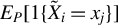 , which prioritizes matching behavior at
$X_i$
 values which are more common in the population.
$\triangle $

The pseudo-true parameter corresponds to the identified set with
$d^2=J_W(P):$
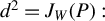

Hence, if a researcher assumes that the true parameter value is equal to the pseudo-true parameter, this is the same as assuming that the degree of misspecification, measured in the norm
$\|\cdot \|_W$
 , is as small as it can possibly be given the observed distribution P.Footnote
3
If they instead allow the possibility that
$\theta $
 and
$\theta _W(P)$
 are different, then as discussed in the introduction, it is not obvious how, if at all, the pseudo-true value
$\theta _W(P)$
 relates to the economic questions that motivate the analysis in the first place. Consequently, it is unclear when we would want to estimate pseudo-true values. The following two sections address this question by providing conditions under which optimal decisions depend on the data through (i) the population minimum distance objective
$Q_W(\theta ;P)$
 and (ii) the pseudo-true value
$\theta _W(P)$
 in particular.
3 OPTIMAL DECISIONS AND MINIMUM DISTANCE
Researchers are often interested in estimating economic parameters in order to inform decisions by policymakers, businesses, or households. It is not obvious that pseudo-true values are suitable for this purpose. To explore this question, we adopt a decision-theoretic perspective and ask under what conditions Bayesian decision-makers would be willing to base decisions on the minimum distance objective and pseudo-true value.
3.1 Decision Problem
Consider a decision-maker who has to choose an action a from a set of possible actions
$\mathcal {A}$
 . After choosing action
$a,$
 the decision-maker suffers a loss
$L(a,\theta )$
 that depends on the action taken and the true value for
$\theta .$
 If
$\theta $
 were known, the optimal action for the decision-maker would be to simply choose
$a\in {\mathrm{arg\,min}}_{a\in \mathcal {A}}L(a,\theta ).$

In fact,
$\theta $
 is unknown and the decision-maker instead observes only the distribution
$P\in \mathcal {P}$
 of the data. Hence, the decision-maker selects a decision rule
$\delta :\mathcal {P}\to \mathcal {A}$
 mapping data distributions into actions. The decision-maker prefers rules
$\delta $
 that yield a lower loss,
$L(\delta (P),\theta ),$
 but when
$\theta $
 cannot be uniquely determined based on P (e.g., when
$\theta $
 is set-identified due to model misspecification), different decision rules
$\delta $
 will perform best at different
$(\theta ,P)$
 pairs, and there generally will not be a uniformly best choice.
One way to choose
$\delta $
 is to consider Bayes decision rules, which weight losses across different
$(\theta ,P)$
 pairs according to a prior
$\pi \in \Delta (\mathbb {R}^p\times \mathcal {P})$
 (i.e., a joint distribution over the parameter of interest and the data distribution). A Bayes decision rule
$\delta _\pi $
 minimizes the average loss under the prior:

To compute
$\delta _\pi $
 , it suffices to minimize the posterior expected loss at each
$P:$


where we assume for simplicity that the posterior for
$\theta |P$
 is continuous and write
$\pi (\theta | P)$
 for the posterior density.
Example: Linear IV (Continued)
Suppose the decision-maker needs to set a tax or subsidy
$a\in \mathbb {R}$
 for the treatment, where
$a>0$
 denotes a subsidy, while
$a<0$
 denotes a tax, and that the loss is
$L(a,\theta )=(a-\theta )^2$
 . That is, the optimal subsidy level is equal to the ATE, while the loss increases quadratically as the subsidy departs from the ATE. This loss arises naturally when demand for treatment varies linearly with the subsidy amount.
$\triangle $

3.2 Minimum-Distance Priors
The posterior density
$\pi (\theta |P)$
 summarizes all decision-relevant information about the parameter
$\theta $
 given the data. To connect minimum distance methods and Bayes decision rules, we consider a class of decision-makers for whom the minimum distance objective function is a sufficient statistic, in the specific sense that
$\pi (\theta |P)$
 is proportional to a function of
$(Q_W(\theta ;P),W(P),\theta ).$
 For such priors, the minimum distance objective contains all
$\theta $
 -relevant information and so is the natural basis for decision-making.
Assumption 1. The conditional prior
$\pi (Y(P),\theta |X(P),W(P))$
 is absolutely continuous with full support and a continuous density for all
$X(P),W(P)$
 . Moreover, for all
$P\in \mathcal {P}$
 and
$\theta \in \mathbb {R}^p$
 ,

for a nonnegative function h that is twice continuously differentiable in Q and continuously differentiable in
$\theta $
 , with a constant of proportionality
$c(P)$
 determined by
$\int \pi (\theta |P)d\theta =1$
 .
The first part of the assumption is imposed for convenience and could be weakened. The second part of the assumption connects the posterior distribution to the minimum distance objective and is weaker than assuming
$\pi (\theta |P)$
 is proportional to a function
$h(Q_W(\theta ;P),\theta )$
 as in the Gibbs posterior distributions studied in the statistics and machine learning literature (e.g., Catoni, Reference Catoni2007; Alquier, Ridgway, and Chopin, Reference Alquier, Ridgway and Chopin2016; Bissiri, Holmes, and Walker, Reference Bissiri, Holmes and Walker2016; Martin and Syring, Reference Martin, Syring, Rao, Young and Rao2022) and the quasi-Bayesian approach of Chernozhukov and Hong (Reference Chernozhukov and Hong2003). Under Assumption 1, providing the decision-maker with
$(Q_W(\cdot ;P), W(P))$
 is as good as providing them with the full data. By contrast, when Assumption 1 fails, the minimum distance objective fails to summarize the implications of P for
$\theta $
 and minimum distance methods may be inappropriate. Hence, we view Assumption 1 as a reasonable restriction in settings where Bayesian decision-makers are considering minimum distance methods.
Assumption 1 immediately implies that the posterior density
$\pi (\theta |P)$
 depends on the data only through
$(W(P), X(P), Y(P))$
 .
Lemma 1. Under Assumption 1,
$\pi (\theta | P)=\pi (\theta | W(P), X(P), Y(P))$
 for all
$P\in \mathcal {P}$
 . Proofs for all results are collected in the Appendix.
Example: Linear IV (Continued)
Focusing on the case where
$W(P)$
 is the TSLS weighting matrix
$W(P)=E_P[Z_iZ_i']^{-1},$
 Lemma 1 implies that the decision-maker’s posterior for the ATE depends on the data only through the reduced-form and first-stage regression coefficients, together with the covariance matrix of the instruments. This rules out, for instance, situations where the decision-maker’s beliefs about the ATE are informed by higher moments of P.
$\triangle $

Assumption 1 further implies that the posterior density
$\pi (\theta | P)$
 can be expressed in terms of the minimum distance moments (1). In particular, the first part of Assumption 1 implies that the conditional priors for
$\theta $
 given
$(W(P),X(P))$
 and
$\eta $
 given
$( W(P), X(P),\theta )$
 are continuous. For brevity, let
$\pi _\theta (\theta )=\pi (\theta |W(P),X(P))$
 and
$\pi _\eta (\eta | \theta )=\pi (\eta |W(P),X(P),\theta )$
 denote their densities with respect to Lebesgue measure. The posterior density of
$\theta $
 given P is then

This resembles the posterior in a finite-sample problem with parameter
$\theta ,$
 prior
$\pi _\theta ,$
 and likelihood
$\pi _\eta .$
 Consistent with this resemblance, the posterior
$\pi (\theta |P)$
 will be non-degenerate with non-trivial uncertainty about the true value of
$\theta $
 even though the data distribution P in our problem is perfectly known. This reflects the fact that
$\theta $
 is not point-identified once
$\eta $
 is unknown, so when the conditional prior
$\pi _\eta $
 is non-dogmatic the decision-maker remains uncertain about
$\theta $
 even after observing
$P.$

Under restrictions on the misspecification prior
$\pi _\eta (\eta |\theta )$
 , Assumption 1 further implies that the prior density at
$\eta $
 conditional on
$(\theta ,W(P))$
 depends only on
$\eta 'W(P)\eta $
 ,
$\pi _\eta (\eta |\theta )\propto f(\eta 'W(P)\eta |\theta , W(P))$
 .
Assumption 2. The conditional prior
$\pi _\eta (\eta |\theta )= \pi (\eta |\theta , W(P), X(P)):$

-
(i) is strictly positive and twice continuously differentiable in $\eta $
 and
$\theta $
,
-
(ii) does not depend on $X(P)$
:
$\pi (\eta |\theta , W(P), X(P)) = \pi (\eta |\theta , W(P))$
for all
$X(P)$
, and -
(iii) has conditional mean zero given $W(P)$
,
$E_\pi [\eta | \theta ,W(P)] = \int \eta \pi _\eta (\eta |\theta )d\eta = 0$
.






Moreover,
$\mathcal {P}$
 is sufficiently rich that we can freely vary
$(Y(P),X(P))$
 while holding
$W(P)$
 fixed.
Assumption 2(i) requires that the conditional prior on misspecification be sufficiently smooth. Assumption 2(ii) further requires that it not depend on the Jacobian matrix
$X(P)$
 , and thus that
$X(P)$
 and
$\eta $
 be conditionally independent given
$(\theta ,W(P))$
 under the prior. In the context of linear IV, for instance, this requires that the researcher not update about the violation of the model’s overidentifying restrictions based on the observed first stage. Assumption 2(iii) further requires that
$\eta $
 have conditional mean zero under the prior given
$W(P),$
 so the researcher thinks that the model is “right on average” even after observing the weighting matrix. To simplify the proof, we further assume that we can freely vary
$(Y(P),X(P)).$

Lemma 2. Under Assumptions 1 and 2, the conditional prior density
$\pi _\eta (\eta | \theta )$
 is rotationally invariant with respect to
$W(P)$
 , taking the form

Lemma 2 implies that the prior density
$\pi _\eta (\eta | \theta )$
 is invariant to rotation of
$W(P)^{\frac {1}{2}}\eta ,$
 in the sense that for any
$\eta , \tilde \eta $
 such that
$W(P)^{\frac {1}{2}}\eta =O W(P)^{\frac {1}{2}}\tilde \eta $
 for an orthonormal matrix
$O,$
 the prior density is the same at
$\eta $
 and
$\tilde \eta $
 ,
$\pi _\eta (\eta | \theta )=\pi _\eta (\tilde \eta | \theta )$
 . The density
$\pi _\eta (\eta | \theta )$
 is thus constant on the ellipsoids
$\{\eta :\eta 'W(P)\eta =C\}$
 for all C, from which it follows that
$\pi _\eta (\eta | \theta )$
 is an elliptically contoured distribution (see Muirhead, Reference Muirhead1982, Chap. 1.5).
Example: Linear IV (Continued)
Recall that
$\eta =(\beta - \theta \cdot \iota ) \circ E_P[Z_iX_i]$
 measures the difference between the ATE and the vector of one-instrument-at-a-time IV estimands. One example of an elliptically contoured distribution in this setting takes
$\eta |\theta ,W(P)\sim N(0,W(P)^{-1})$
 , which corresponds to
$f(u|\theta , W(P))\propto \exp (-\frac {1}{2}u)$
 . Under this prior, each single-instrument estimand is equal to the ATE plus a mean-zero noise term, where the covariance matrix of the noise is determined by
$W(P)$
 and the first stage
$E_P[Z_iX_i].$
 There are many other rotation-invariant priors, however, including a multivariate t prior with
$\nu $
 degrees of freedom, where
$ f(u|\theta , W(P))\propto \left (1+\frac {1}{\nu }u\right )^{-\frac {\nu +k}{2}}.\ \triangle $

Lemma 2 implies that, under the conditions of Assumption 2, the posterior density
$\pi (\theta |P)$
 is proportional to a function of
$(Q_W(\theta ;P),W(P),\theta ),$
 as required by Assumption 1, only if the (conditional) prior on
$\eta $
 is rotation-invariant. In fact, rotation-invariance is both necessary and sufficient for Assumption 1 in settings where Assumption 2 holds.
Proposition 1. Under Assumption 2, Assumption 1 holds if and only if for all
$P\in \mathcal {P},$
 the conditional prior
$\pi (Y(P),\theta |X(P),W(P))$
 is absolutely continuous and

for a nonnegative function
$f(u|\theta , W(P))$
 with
$\int f(\eta '\eta |\theta , W(P))d\eta < \infty .$

We have thus shown that, under the conditions on
$\eta |\theta ,W(P),X(P)$
 imposed by Assumption 2, the minimum distance objective is sufficient in the sense of Assumption 1 if and only if our misspecification priors
$\pi _\eta $
 are rotation-invariant. Hence, for such priors, it is natural to focus on the minimum distance objective and, conversely, a focus on the minimum distance objective is most reasonable under such priors. Justifying a focus on the pseudo-true value, that is, on the argmin of the minimum distance objective, requires further restrictions, which we turn to next.
4 CONCENTRATION-INDUCING PRIORS
As shown in the last section, for a fixed prior
$\pi (\theta ,P)$
 satisfying Assumptions 1 and 2, we obtain a non-degenerate posterior
$\pi (\theta |P),$
 and so are uncertain about the parameter
$\theta $
 even though the data distribution P is perfectly known. Plug-in decision rules based on the pseudo-true parameter value, by contrast, correspond to Bayes decision rules in the case where our posterior is a point mass at
$\theta _W(P).$
 We next characterize sequences of priors satisfying Assumptions 1 and 2 such that the corresponding posterior sequences concentrate at
$\theta _W(P)$
 . Under such prior sequences, the plug-in approach is correct in the limit, justifying a focus on the pseudo-true parameter.
While these prior sequences rationalize a focus on the pseudo-true value, we find them unsatisfactory in several respects. First, these sequences assume that the model is misspecified with probability one (in the sense that
$\|\eta \|_{W}>0$
 almost surely under the prior), but take the expected magnitude of misspecification to zero. Hence, while these priors allow the possibility of misspecification, they assume that the degree of misspecification is arbitrarily small. An assumption that the degree of misspecification is very small seems unreasonable in many economic applications. Second, we show that concentration around the pseudo-true value is fragile in important respects. If we take our concentration-inducing prior sequences and mix them, to an arbitrarily small degree, with any fixed full-support prior on
$\eta |\theta $
 , concentration around the pseudo-true value immediately fails whenever
$J_W(P)>0$
 . Moreover, even under prior sequences which imply a vanishing degree of misspecification, concentration around the pseudo-true value requires that the prior on
$\eta $
 be sufficiently thin-tailed.
4.1 Posterior Concentration
Our sufficient conditions for posterior concentration require that the prior density for
$W(P)^{\frac {1}{2}}\eta $
 be independent of
$(\theta ,W(P))$
 and thin-tailed, in the sense that
$f(\eta 'W(P)\eta |\theta ,W(P))$
 decays at a faster-than-polynomial rate as
$\eta 'W(P)\eta \to \infty .$

Assumption 3. For
$f(\eta 'W(P)\eta |\theta ,W(P))$
 as defined in Lemma 2 and all
$(\theta ,W(P))$
 ,
$f(u|\theta ,W(P))\propto f(u),$
 where
$f(u)$
 is strictly positive, continuous, and non-increasing in u, and satisfies
$\lim _{u\to \infty }\frac {f(au)}{f(u)}=0$
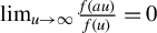 for all
$a>1$
 .
This assumption holds, for instance, when
$\pi (\eta |\theta )$
 is normal with variance proportional to
$W(P)^{-1}$
 .
Example: Linear IV (Continued)
If
$\pi _{\eta }(\eta |\theta )$
 is an
$N(0,W(P)^{-1})$
 density, then since
$\exp \left (-\frac {a}{2}u\right )/\exp \left (-\frac {1}{2}u\right )=\exp \left (\frac {1-a}{2}u\right )$
 and
$a>1,$
 Assumption 3 holds.
$\triangle $

Under sequences of priors that (i) satisfy Assumptions 1–3 and (ii) take the degree of misspecification to be small a priori, the posterior concentrates on the pseudo-true value. Formally, we consider a scale family of priors on the misspecification parameter
$\eta , \pi _{\eta ,c}(\eta |\theta )\propto f(\frac {1}{c}\eta 'W(P)\eta ),$
 where the scale parameter c controls the magnitude of misspecification and the prior variance of
$\eta $
 scales with c. Our main result in this section considers posterior behavior as the scale parameter becomes small,
$c\to 0$
 , corresponding to priors that assume a vanishing degree of misspecification.
Proposition 2. Suppose Assumptions 1–3 hold. For any continuous
$\pi _\theta (\theta )$
 with
$\pi _\theta (\theta _W(P))>0,$
 the posterior

concentrates on
$\theta _W(P)$
 as
$c\to 0$
 , in that for
$B_\varepsilon (\theta _W(P))=\left \{\theta :\Vert \theta _W(P)-\theta \Vert <\varepsilon \right \}$
 ,

Proposition 2 shows that for priors satisfying Assumptions 1–3 where the degree of misspecification is small, the posterior distribution concentrates on
$\theta _W(P).$
 This is entirely expected when
$J_W(P)=0$
 , since, in this case, the data provide no evidence of misspecification and priors with
$c\to 0$
 assume the model is nearly correct. When
$J_W(P)>0,$
 by contrast, the data imply non-trivial misspecification but Proposition 2 shows that the posterior continues to concentrate.
Concentration of
$\pi _c(\theta |P)$
 implies convergence of the Bayes decision rule

under conditions on the decision problem.
Proposition 3. Suppose that
$\mathcal {A}$
 is compact under some metric d, that
$\sup _{a,\theta }L(a,\theta )<\infty $
 , that
$\sup _{\theta }|L(a,\theta )-L(a',\theta )|<\lambda \cdot d(a,a')$
 for all
$a, a'\in \mathcal {A}$
 and some
$\lambda>0$
 , that
$L(a,\cdot )$
 is continuous for all
$a\in \mathcal {A}$
 , and that the loss
$L(a,\theta )$
 has a unique minimum for all
$\theta $
 . Then as
$c\to 0, \delta _{\pi _c}(P)\to {\mathrm{arg\,min}}_{a\in \mathcal {A}}L(a,\theta _W(P)). $

Proposition 3 shows that for bounded loss functions that are Lipschitz in a and continuous in
$\theta ,$
 Bayes decision rules corresponding to the priors we study converge to plug-in decision rules based on the pseudo-true value. This result is useful for a number of reasons. First, it shows that plug-in decision rules using the pseudo-true parameter value correspond to the limit of a sequence of Bayes decision rules for a large class of loss functions, providing one justification for such rules. Second, it shows that the pseudo-true parameter value
$\theta _W(P)$
 is a sufficient statistic for communication with an audience whose priors take the limiting form we consider: a researcher looking to summarize the data for such an audience is justified in reporting only the pseudo-true parameter value, since it allows audience members to compute the optimal decision for whatever loss function they have, provided that loss satisfies the conditions of Proposition 3.
The conditions in Proposition 3 are somewhat restrictive and rule out squared error loss on an unbounded domain. These conditions are sufficient but not necessary, however, and we can obtain convergence of decision rules in many other settings by using additional structure for the loss function and prior.
Example: Linear IV (Continued)
Proposition 3 does not apply in this example, because the loss
$L(a,\theta )=(a-\theta )^2$
 is neither bounded nor Lipschitz. Nonetheless, if
$\pi _\eta (\eta |\theta )$
 corresponds to an
$N\left (0,\left (\frac {1}{c}W(P)\right )^{-1}\right )$
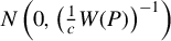 distribution while the prior on
$\theta $
 is flat, the posterior density is

Hence, for all
$c,$
 the posterior distribution is, normal centered at
$\theta _W(P)$
 with variance proportional to c. Consistent with Proposition 2, this posterior converges weakly to a point mass at
$\theta _W(P)$
 as
$c\to 0$
 . Moreover, despite the conditions of Proposition 3 not holding in this example, the Bayes decision rule
$\delta _{\pi _c}(P)$
 is equal to
$\theta _W(P)$
 for all
$c.\ \triangle $

4.2 Posterior Concentration Is Fragile
While we have shown that the plug-in decision rule using the pseudo-true value corresponds to the limit of Bayes decision rules for certain sequences of priors, we think this justification carries limited weight, for multiple reasons. For one, the prior sequences used to establish convergence assume the degree of misspecification is negligible a priori, which seems difficult to justify in many economic applications. Moreover, as we next show, the convergence established by Propositions 2 and 3 is fragile in important respects.
4.2.1 Fragility to Prior Contamination
If we mix the concentration-inducing priors studied in the previous section with any fixed, full-support prior for
$\eta |\theta $
 , posterior concentration fails when
$J_W(P)>0.$

Proposition 4. Consider conditional priors of the form

for any conditional prior
$\pi ^*_\eta (\eta |\theta )$
 with strictly positive density and
$\phi \in (0,1)$
 . Suppose Assumption 3 holds. If
$J_W(P)>0$
 , then, for any
$\pi _\theta (\theta ),$
 the resulting posterior satisfies

If instead
$J_W(P)=0$
 ,
$\pi _\theta (\theta )$
 is continuous, and
$\pi _\theta (\theta _W(P))>0,$
 then

Proposition 4 shows that if
$J_W(P)>0$
 and we contaminate the concentration-inducing prior
$\pi _{\eta ,c}(\eta |\theta ),$
 to an arbitrarily small extent, with any full-support prior
$\pi _\eta ^*$
 for
$\eta |\theta ,$
 then the posterior converges to the same limit as if we had set
$\pi _\eta (\eta |\theta )=\pi ^*_\eta (\eta |\theta )$
 . By contrast, when
$J_W(P)=0,$
 the contaminated posterior continues to concentrate on
$\theta _W(P)$
 as
$c\to 0.$
 In this case, the concentration-inducing component
$\pi _{\eta ,c}(\eta |\theta )$
 receives asymptotically all of the posterior weight, despite the contamination by
$\pi _\eta ^*(\eta |\theta )$
 .
Proposition 4 can be interpreted in terms of pre-testing for model specification: in the case where
$J_W(P)>0,$
 the data imply that the model is non-trivially misspecified. While the priors
$\pi _{\eta ,c}(\eta |\theta )$
 imply that the model is misspecified with probability one, as
$c\to 0,$
 they imply that the degree of misspecification is arbitrarily small. When we allow the possibility that
$\eta $
 is instead drawn from a fixed full-support distribution
$\pi ^*_\eta ,$
 for c sufficiently small, the data provide arbitrarily strong support for
$\pi ^*_\eta (\eta |\theta )$
 over
$\pi _{\eta ,c}(\eta |\theta )$
 . Loosely speaking, the concentration-inducing prior
$\pi _{\eta ,c}(\eta |\theta )$
 is rejected in favor of the full-support prior
$\pi ^*_\eta (\eta |\theta )$
 .Footnote
4
4.2.2 Fragility to Heavy Tails
Even under prior sequences such that the degree of misspecification goes to zero, the concentration obtained in Proposition 2 relies on thin tails for
$\pi _\eta (\eta |\theta )$
 . To illustrate this point, we show that posterior concentration around the pseudo-true value fails in two examples with heavy-tailed priors.
Example: Posterior Non-Concentration with t Prior
Suppose that our prior on
$\eta $
 corresponds to a multivariate t distribution centered at zero with scale matrix
$W(P)^{-1}$
 and
$\tilde \nu $
 degrees of freedom,
$f(u) \propto \left (1 + \frac {1}{\tilde \nu }u\right )^{-\frac {\tilde \nu + k}{2}}$
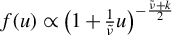 . Provided
$J_W(P)>0,$
 if we define
$\nu =\tilde \nu + k - p$
 and

one can show that

where the second term is the density for a multivariate t distribution centered at
$\theta _W(P)$
 , with scale matrix
$\Sigma (P)$
 and
$\nu $
 degrees of freedom. Consequently, the
$c\to 0$
 limiting posterior corresponds to updating the prior
$\pi _\theta $
 based on observing
$\theta _W(P)\sim t_{{\nu }}(\theta ,\Sigma (P)).$

Note that the degrees of freedom in the “likelihood,”
$\nu $
 , are equal to the degrees of freedom in the misspecification prior
$\pi _\eta $
 plus the degree of over-identification, so a higher degree of over-identification leads to thinner tails for the posterior, all else equal. The scale parameter in the “likelihood,”
$\Sigma (P) = J_W(P) \left ({\nu } X(P)'W(P)X(P)\right )^{-1}$
 , is increasing in the J-statistic so cases where the moment conditions are observed to be more badly violated lead to a more uncertain posterior, all else equal.
$\triangle $

The tail thickness of
$f(\cdot )$
 matters because it determines beliefs about the total level of misspecification conditional on a given value of the J-statistic. To see this, let us again assume that
$\eta |\theta \sim \pi _{\eta ,c}(\eta |\theta )$
 and consider the conditional distribution of
$\|\eta \|_W$
 conditional on the norm of
$\eta $
 exceeding a threshold
$\tau $
 ,
$\|\eta \|_W|\left (\tau \leq \|\eta \|_W\right )$
 . For thin-tailed priors (i.e., those satisfying Assumption 3), one can show that, for all
$a>1$
 and all positive constants
$\tau>0$
 ,

Hence, even in the case where the model is known to be misspecified, as
$c\to 0,$
 thin-tailed priors imply that the degree of additional misspecification, beyond that implied by the lower bound
$\tau $
 , is negligible. Recall, however, that the J-statistic is itself a lower bound on the total degree of misspecification,
$\|\eta \|_W^2\ge J_W(P)$
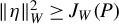 . Consistent with this, when
$c\to 0,$
 thin-tailed priors imply that the total degree of misspecification must not be much larger than that suggested by the J-statistic, and thus that
$\theta $
 must be close to
$\theta _W(P),$
 the unique parameter value compatible with
$\|\eta \|_W^2=J_W(P).$

By contrast, for f corresponding to a multivariate t distribution, we have that

for a fixed, nonzero function
$p(\cdot )$
 that does not depend on
$\tau $
 . Consequently, in this case, the researcher’s belief about the total degree of misspecification is non-degenerate and, once c is sufficiently small, scales proportionally with
$\tau .$

While t-distributed priors for
$\eta |\theta $
 correspond to updates via a t likelihood in the
$c\to 0$
 limit, if we instead consider a multivariate power law prior for
$\eta |\theta ,$
 then dependence on c vanishes entirely.
Example: Posterior Non-Concentration with Power Law Prior
Suppose
$f(x) \propto x^{-\alpha }$
 for
$\alpha> p/2$
 (noting that this is improper). Then for
$\nu =2\alpha -p$
 ,

and for all
$c,$


which corresponds to the posterior distribution from observing
$\theta _W(P)\sim t_\nu (\theta ,\Sigma (P))$
 . We again see that a higher degree of over-identification leads to thinner tails for the posterior, while a larger J-statistic leads to a more dispersed posterior.
$\triangle $

5 CONFIDENCE SETS BASED ON ROTATION-INVARIANCE
When
$\pi (\theta |P)$
 does not concentrate on the pseudo-true value, researchers will have non-trivial uncertainty about the true value of
$\theta $
 even after observing P, and the exact posterior will depend on the details of the prior. Despite this dependence on the prior, we show that there nonetheless exist confidence intervals with correct ex-ante coverage for the true value
$\theta $
 under all priors satisfying Assumptions 1 and 2. Since we previously argued that this class of priors has a close connection to minimum distance methods, we view these confidence sets as a natural summary for misspecification-driven uncertainty in settings where researchers adopt a minimum distance approach.
To state this result, suppose the researcher is interested in inference on a linear combination of the elements of
$\theta , v'\theta $
 for
$v\in \mathbb {R}^p.$
 For
$t_{k-p, 1-\frac {\beta }{2}}^*$
 the level
$1-\frac {\beta }{2}$
 critical value for a standard t distribution with
$k-p$
 degrees of freedom,
$\theta _{W}\left (P\right )={\mathrm{arg\,min}}_{\theta }Q_W(\theta ;P)$
 the pseudo-true value,
$J_W(P)=\min _\theta Q_W(\theta ;P)$
 the population J-statistic, and

a transformation of the Hessian of the population minimum distance objective, define the confidence interval

This interval has correct coverage conditional on
$(W(P),X(P))$
 , and thus correct ex-ante coverage, under priors satisfying Assumptions 1 and 2.
Proposition 5. For any prior
$\pi $
 such that Assumptions 1 and 2 hold,

The confidence interval (7) has a number of interesting features. It is centered at the pseudo-true value and its width is governed by (i) the Hessian of the minimum distance objective function
$\frac {\partial ^2}{\partial \theta \partial \theta '}Q_W(\theta ;P)$
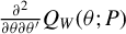 and (ii) the population J-statistic
$J_W(P).$
 The fact that a smaller Hessian leads to wider confidence intervals resembles many other inference problems, though ours is unusual in that it is derived in a population setting and reflects uncertainty due to misspecification, rather than sampling uncertainty. The dependence on the population J-statistic is also unusual, though intuitively reasonable given the connection to model misspecification.
The notion of coverage considered in Proposition 5 is non-standard. Since P is observed in our setting, the frequentist coverage is either zero or one,
$Pr_{(\theta ,P)}\left \{v'\theta \in CI(P)\right \}\in \{0,1\}.$
 Proposition 5 instead considers average coverage under
$\pi :$


which measures the ex-ante coverage probability under the prior. Proposition 5 thus establishes that any Bayesian whose prior satisfies Assumptions 1 and 2 thinks, before seeing the data, there is a
$1-\beta $
 probability that
$CI(P)$
 will cover
$v'\theta $
 .Footnote
5
In this sense, the interval (7) has correct average coverage under any prior satisfying Assumptions 1 and 2.
We provide intuition for Proposition 5 from two perspectives, first establishing a connection to generalized least squares and then showing that
$CI(P)$
 corresponds to a credible set under an improper power law prior.
Regression Interpretation
Note that, for

we can write the minimum distance model allowing for misspecification, as

where, under priors
$\pi $
 satisfying Assumptions 1 and 2, the conditional distribution of
$\tilde {\eta }|\tilde {X}(P),\theta $
 is rotation-invariant:

for all orthonormal matrices O. Hence, for any prior satisfying Assumptions 1 and 2, the problem of inference on
$\theta $
 conditional on
$\tilde {X}(P)$
 reduces to that of inference on the coefficient in a regression with a rotation-invariant error. However, the t-distribution for t-statistics holds whenever the error distribution is rotation-invariant, while (7) is exactly the t-statistic confidence interval derived from (8) and so is valid under any prior satisfying Assumptions 1 and 2.Footnote
6
Bayesian Interpretation
Recall that under the (improper) multivariate power law prior for
$\eta |\theta $
 ,
$f(x) \propto x^{-\alpha }$
 , the posterior
$\pi _c(\theta |P)$
 corresponds to a t distribution with
$2\alpha -p$
 degrees of freedom. Consequently, the confidence interval (7) corresponds to a posterior credible set under a flat prior on
$\theta $
 and a multivariate power law prior on
$\eta $
 with
$\alpha =k/2.$
 Viewed from this perspective, Proposition 5 shows that there exists an improper conditional prior on
$\theta ,\eta |W(P),X(P)$
 whose credible sets have correct average coverage under all priors satisfying Assumptions 1 and 2.
5.1 Comparison to Norm-Bound Identified Sets
We next compare the behavior of the confidence set (7) to the identified set (3) constructed under the bound
$\|\eta \|_W\le d.$
 To facilitate this comparison, note that

for

the projection matrix onto
$\tilde X(P)=W(P)^{\frac {1}{2}}X(P)$
 . Here,
$\hat \eta $
 and
$\eta ^\perp $
 are the projection of
$\tilde \eta $
 onto the column span of
$\tilde X(P)$
 and the residual from this projection, respectively. By definition
$\|\eta ^\perp \|^2=J_W(P)$
 , so the J-statistic measures the length of the projection residual, while
$\hat \eta =\tilde {X}(P)(\theta _W(P)-\theta )$
 governs the difference between the true and pseudo-true parameter values. Intuitively,
$\eta ^\perp $
 is the detectable component of the misspecification vector
$\eta $
 , which has no effect on the bias of the pseudo-true value but governs the J-statistic. Analogously,
$\hat \eta $
 is the undetectable component, which governs the bias but has no effect on the J-statistic. The overall degree of misspecification reflects the sum of these terms,
$\|\eta \|_W^2=\|\eta ^\perp \|^2+\|\hat \eta \|^2$
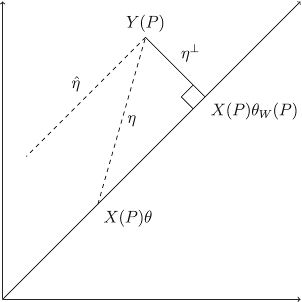
 . Figure 1 visualizes this decomposition in a case where
$\theta $
 is scalar.
Relationship between the pseudo-true value
$\theta_W(P) $
 and true parameter value
$\theta $
 in an example with scalar
$\theta .$
 The solid diagonal line represents the column space of
$X(P)$
 . The vector
$\eta ^\perp $
 perpendicular to the column space captures the detectable component of the misspecification vector, while vector
$\hat \eta $
 parallel to the column space captures the undetectable component of misspecification.

Equipped with this decomposition, note that, for
$\hat \eta (\theta ,P),$
 the undetectable misspecification component implied by
$(\theta ,P)$
 ,

we can write the identified set for
$\theta $
 as

This implies an identified set for
$v'\theta $
 equal to

Hence, the bounds of the identified set correspond to values of
$\theta $
 which spend the misspecification “budget”
$\|\hat \eta (\theta ,P)\|^2\le d^2-J_W(P)$
 obtained by subtracting the J-statistic from the a priori upper bound
$d^2.$
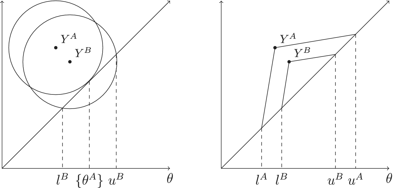
 As the degree of detectable misspecification becomes more severe, in the sense that the J-statistic grows larger, the length of the identified set shrinks. The first panel of Figure 2 illustrates this, again focusing on the case where
$\theta $
 is scalar. Here, we hold d,
$X(P),$
 and
$W(P)$
 fixed but consider two possible values
$Y(P), Y^A$
 and
$Y^B,$
 where
$Y^A$
 implies a larger J-statistic. The identified set for
$\theta $
 is larger for
$Y^B$
 than
$Y^A.$
 Indeed, the J-statistic at
$Y^A$
 is exactly equal to
$d^2,$
 so the identified set collapses to the pseudo-true parameter value. Note that while the identified sets implied by the misspecification bounds in, for example, Armstrong and Kolesár (Reference Armstrong and Kolesár2021) can exhibit these comparative statics, for inference that paper recommends “fixed length” confidence intervals which, as the name suggests, have fixed length and so avoid this issue.
Intervals for
$\theta $
 using the norm-bounding approach and the rotation-invariant prior approach. When dataset A or B is observed, the identified set or confidence interval for
$\theta $
 is given by
$[l^A, u^A]$
 or
$[l^B, u^B]$
 , respectively, where in the left panel
$l^A=u^A=\theta ^A$
 .
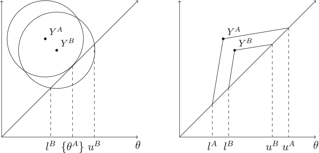
Figure 2 Long description
A multi-panel figure with two side-by-side graphs. Both graphs feature a horizontal axis labeled theta and a vertical axis with no label. A diagonal line bisects each graph from the origin to the top right.
Left Panel: Norm-bounding approach.
Two overlapping circles are centered at points Y super A and Y super B. Y super A is positioned higher and further left than Y super B. Vertical dashed lines drop from the intersection points of the circles and the diagonal line to the horizontal axis. These points on the theta axis are labeled l sub B, followed by a set containing theta super A, and finally u sub B. The point theta super A corresponds to the single point where the circle for dataset A is tangent to the diagonal line.
Right Panel: Rotation-invariant prior approach.
Two nested, irregular quadrilateral shapes are anchored to the diagonal line, representing datasets A and B. The outer shape is associated with Y super A and the inner shape with Y super B. Vertical dashed lines drop from the vertices where these shapes meet the diagonal line down to the horizontal axis. From left to right, the labels on the theta axis are l sub A, l sub B, u sub B, and u sub A.
In contrast to the identified set
$\Theta _I(P,d)$
 , our proposed confidence intervals are wider for larger values of
$J_W(P)$
 . We can re-write the interval (7) as

As the second panel of Figure 2 illustrates, the width of this interval is increasing in the size of the J-statistic, with a wider interval for
$Y^A$
 than for
$Y^B.$
 This seems like a potentially appealing property for uncertainty summaries in settings where researchers are concerned about misspecification.
5.2 Confidence Intervals in Finite Samples
So far, our results have abstracted from sampling uncertainty, considering the setting where P is observed directly. While our analysis of estimands is fundamentally tied to this setting, our construction of confidence intervals extends naturally to settings with sampling uncertainty.
Formally, now suppose the researcher observes a finite sample
$D^n=(D_1,\ldots ,D_n)$
 and considers linear-in-parameters sample moment conditions

where
$Y_n$
 ,
$X_n$
 , and
$g_n(\theta )$
 are the finite-sample counterparts of
$Y(P)$
 ,
$X(P)$
 , and
$g(\theta ;P),$
 respectively. At the true
$\theta $
 , define
$\eta _n = g_n(\theta )$
 . In this setting,
$\eta _n$
 aggregates both population-level misspecification and the sampling noise of the moments. Further define
$W_n$
 as the finite-sample counterpart of
$W(P)$
 and
$Q_{n}(\theta )= \Vert Y_n - X_n \theta \Vert _{W_n}^2$
 . We impose analogs of Assumptions 1 and 2.
Assumption 4. The conditional prior
$\pi (Y_n,\theta |X_n,W_n)$
 is absolutely continuous with full support and a continuous density for all
$X_n,W_n$
 . Moreover, for all
$D^n$
 and
$\theta \in \mathbb {R}^p$
 ,

for a nonnegative function h that is twice continuously differentiable in Q and continuously differentiable in
$\theta $
 , with a constant of proportionality
$c(D^n)$
 .
Assumption 5. The conditional prior
$\pi _{\eta _n}(\eta _n|\theta )=\pi (\eta _n|\theta , W_n, X_n)$
 :
-
(i) is strictly positive and twice continuously differentiable in $\eta _n$
and
$\theta $
, -
(ii) does not depend on $X_n$
:
$\pi (\eta _n|\theta , W_n, X_n) = \pi (\eta _n|\theta , W_n)$
for all
$X_n$
, and -
(iii) has conditional mean zero given $W_n$
,
$E_\pi [\eta _n | \theta ,W_n] = \int \eta _n \pi _{\eta _n} (\eta _n |\theta )d\eta _n = 0$
.






Moreover, the support of the data is such that we can freely vary
$(X_n,Y_n)$
 while holding
$W_n$
 fixed.
Under these conditions, we obtain a finite-sample analog of Proposition 5. Define

where
$\theta _{n,W_n}, J_{n,{W_n}},$
 and
$\sigma _{v,n}$
 are the finite-sample counterparts of
$\theta _{W}(P)$
 ,
$J_W(P)$
 , and
$\sigma _{v}(P),$
 respectively.


5.3 Confidence Intervals Under Local Misspecification
The last section showed that our confidence sets for linear-in-parameters moment condition models with P observed directly translate to finite-sample results, again for linear-in-parameters models. Standard arguments imply, however, that nonlinear moment condition models are approximately linear in large samples, so long as the degree of misspecification is sufficiently small. Thus, our confidence sets similarly extend to locally misspecified, but potentially nonlinear, models.
To sketch this extension, following Armstrong and Kolesár (Reference Armstrong and Kolesár2021), let us suppose that the sample of size n is generated from a DGP
$P_n$
 where, for a vector of potentially nonlinear moments g, the pair
$(\theta ,P_n)$
 satisfies the local misspecification conditionFootnote
7

Armstrong and Kolesár (Reference Armstrong and Kolesár2021) show that under local misspecification and additional regularity conditions, the problem of constructing a confidence interval for a scalar parameter
$\kappa (\theta )$
 (for some possibly nonlinear function
$\theta \mapsto \kappa (\theta )$
 ) is asymptotically equivalent to the problem of constructing a confidence interval for the parameter
$K\theta $
 (for the
$1\times p$
 derivative matrix of
$\kappa $
 at the true
$\theta $
 given by K) in the approximately linear model

where
$\Gamma _L$
 corresponds to the Jacobian of the moments at the true parameter value and we observe
$Y_L$
 and
$\Gamma _L,$
 while
$\Sigma $
 is known.Footnote
8
Defining
$\eta = \mu + \varepsilon $
 , if our prior on
$\eta $
 is rotation-invariant (as follows, for instance, if we have an
$N(0,\Omega )$
 prior on
$\mu $
 with
$\Omega +\Sigma \propto W^{-1}$
 ), then the limit experiment is isomorphic to a linear regression with rotation-invariant errors. Specifically, for
$X_L = -\Gamma _L$
 , we can re-write the model as

We now state the natural analogs of Assumptions 1 and 2 for this setting, denoting the data in the limit experiment as
$D_L= (Y_L,W_L, X_L)$
 .
Assumption 6. The conditional prior
$\pi (Y_L,\theta |X_L,W_L)$
 is absolutely continuous with full support and a continuous density for all
$X_L,W_L$
 . Moreover, for all
$D_L$
 and
$\theta \in \mathbb {R}^p$
 ,

for a nonnegative function h that is twice continuously differentiable in Q and continuously differentiable in
$\theta $
 , with a constant of proportionality
$c(D_L)$
 determined by
$\int \pi (\theta |D_L)d\theta =1$
 .
Assumption 7. The conditional prior
$\pi _\eta (\eta |\theta )=\pi (\eta |\theta , W_L, X_L)$
 :
-
(i) is strictly positive and twice continuously differentiable in $\eta $
and
$\theta $
, -
(ii) does not depend on $X_L$
:
$\pi (\eta |\theta , W_L, X_L) = \pi (\eta |\theta , W_L)$
for all
$X_L$
, and -
(iii) has conditional mean zero given $W_L$
,
$E_\pi [\eta | \theta ,W_L] = \int \eta \pi _\eta (\eta |\theta )d\eta = 0$
.






Moreover, we can freely vary
$(X_L,Y_L)$
 while holding
$W_L$
 fixed.
Constructing a confidence interval for scalar
$K\theta $
 is then accomplished by defining

for
$\theta _{L,W_L},J_{L,W_L},$
 and
$\sigma _{K,L}$
 the limit experiment counterparts of
$\theta _W(P),J_W(P)$
 , and
$\sigma _v(P),$
 respectively.


6 CONCLUSION
We study the problem of inference in misspecified linear minimum distance models and show that, under restrictions on the prior, (i) a Bayesian decision-maker is content to summarize the data using the minimum distance objective if and only if their prior on model misspecification satisfies a rotation-invariance condition; (ii) a Bayesian is content to further summarize the data via the minimum distance estimand—the pseudo-true value—if their prior on misspecification is thin-tailed and has variance going to zero; and (iii) for any Bayesian with a rotation-invariant prior as in (i), even if the conditions of (ii) don’t hold, a particular confidence set, centered at the pseudo-true value and with width proportional to the square root of a population J-statistic, ensures correct coverage for the true parameter value with no restriction on the magnitude of misspecification.
Informative inference is possible because rotation-invariant priors restrict the “direction” of misspecification, controlling the impact of misspecification on the pseudo-true value relative to the impact on the J-statistic. Our key assumption is that researchers’ choice of weighting matrix reflects their beliefs about the relative likelihood of different kinds of misspecification, which appears consistent with the way in which some researchers already choose their weighting matrices.Footnote 9 For such researchers, our work suggests that a natural way to account for the possibility of model misspecification is by implementing confidence intervals of the form in Section 5, with width that scales with the (population or finite-sample) J-statistic.
FUNDING STATEMENT
This material is based upon work supported by the National Science Foundation Graduate Research Fellowship Program under Grant No. DGE-2140743. Any opinions, findings, and conclusions or recommendations expressed in this material are those of the author and do not necessarily reflect the views of the National Science Foundation.
COMPETING INTERESTS
The authors declare that no competing interests exist.
APPENDIX: PROOFS
Proof of Lemma 1
$Q_W(\cdot; P)$
 can be expressed as a function of
$(X(P), W(P), Y(P))$
 , so by Assumption 1,

as we aimed to show.
$\square $

Proof of Lemma 2
Throughout the proof, we fix an arbitrary positive-definite matrix W and suppress it from the notation; all densities are implicitly conditioned on W. By Assumption 2(ii),
$\pi _\eta (\eta |\theta )$
 does not depend on X, and we write
$\psi (\eta ,\theta ) = \ln \pi _\eta (\eta |\theta )$
 .
Fix any full-rank X and let
$Y = X\theta + \eta $
 . By Bayes’ theorem,

Since
$\pi (Y|\theta ,W,X) = \pi _\eta (Y - X\theta |\theta )$
 by a change of variables, and
$\pi (\theta |Y,W,X) = h(Q_W(\theta ;P),W,\theta )\cdot c(P)$
 by Assumption 1 and Lemma 1, we obtain

where
$A(\eta 'W\eta ,\theta )$
 depends on
$\eta $
 only through
$\eta 'W\eta $
 and does not depend on X;
$B(Y,X)$
 depends on Y and X but not on
$\theta $
 ; and
$S(\theta ,X)$
 depends on
$\theta $
 and X but not on Y. Since the left-hand side
$\psi (\eta ,\theta )$
 does not depend on X by Assumption 2(ii) and A does not depend on X since h takes arguments
$(Q_W, W, \theta )$
 , it follows that
$B(Y,X) + S(\theta ,X)$
 does not depend on X.
We now take mixed partial derivatives to eliminate the nuisance terms B and S. All composed functions are sufficiently smooth that the order of differentiation may be interchanged freely, by Assumptions 1 and 2(i). Differentiating (A.1) with respect to
$\theta $
 (holding
$Y,X,W$
 fixed, so
$\eta = Y - X\theta $
 varies with
$\theta $
 ) and then with respect to
$Y'$
 (holding
$\theta ,X,W$
 fixed) eliminates B and S: the term
$\nabla _\theta B = 0$
 since B does not depend on
$\theta $
 , and
$\frac {\partial }{\partial Y'}\nabla _\theta S = 0$
 since S does not depend on Y. The resulting identity is

where

Since
$\psi $
 does not depend on X by Assumption 2(ii),
$\nabla ^2_{\eta \eta }\psi $
 and
$\nabla ^2_{\eta \theta }\psi $
 do not depend on X. Likewise, G and H do not depend on X, since
$A = \ln h(Q,W,\theta )$
 and
$Q = \eta 'W\eta $
 do not involve X. Defining
$M = \nabla ^2_{\eta \eta }\psi - G$
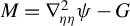 and
$N = \nabla ^2_{\eta \theta }\psi - H$
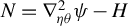 , neither of which depends on X, the identity becomes
$-X'M + N = 0$
 for all X in the open set. For any
$X_0$
 in this set and any sufficiently small perturbation
$\Delta X$
 with
$X_0 + \Delta X$
 still in the set,
$(\Delta X)'M = 0$
 . Taking
$\Delta X = \varepsilon \, e_j e_i'$
 for each
$j\in \{1,\dots ,k\}$
 and
$i\in \{1,\dots ,p\}$
 gives
$(\Delta X)'M = \varepsilon \, e_i\, e_j'\, M = 0$
 ; since this is the outer product of the nonzero vector
$e_i$
 with the row vector
$e_j'M$
 , we obtain
$e_j'M = 0$
 for all j, so
$M = 0$
 and
$N = X_0'M = 0$
 .
The equality
$M = 0$
 means
$\nabla ^2_{\eta \eta }\psi (\eta ,\theta ) = \nabla ^2_{\eta \eta }A(\eta 'W\eta ,\theta )$
 , so
$\nabla ^2_{\eta \eta }[\psi (\eta ,\theta ) - A(\eta 'W\eta ,\theta )] = 0$
 for all
$\eta \in \mathbb {R}^k$
 . A function whose Hessian is identically zero on
$\mathbb {R}^k$
 is affine, so there exist
$\lambda _0(\theta )$
 and
$\lambda _1(\theta )\in \mathbb {R}^k$
 such that

Exponentiating,
$\pi _\eta (\eta |\theta ) = g(\eta ;\theta )\cdot \exp (\lambda _1(\theta )'\eta ),$
 where
$g(\eta ;\theta ) = \exp (A(\eta 'W\eta ,\theta ) + \lambda _0(\theta ))$
 depends on
$\eta $
 only through
$\eta 'W\eta $
 and is therefore an even function,
$g(-\eta ;\theta ) = g(\eta ;\theta )$
 .
It remains to show
$\lambda _1(\theta ) = 0$
 . By Assumption 2(iii),

Pre-multiplying by
$\lambda _1(\theta )'$
 gives

Decomposing
$\mathbb {R}^k$
 into
$S_+ = \{\eta : \lambda _1'\eta> 0\}$
 and
$S_- = \{\eta : \lambda _1'\eta < 0\}$
 (the hyperplane
$\{\lambda _1'\eta = 0\}$
 has measure zero) and substituting
$u = -\eta $
 in the integral over
$S_-$
 , using
$g(-u;\theta ) = g(u;\theta )$
 ,

For
$\eta \in S_+$
 and
$\lambda _1\neq 0$
 :
$\lambda _1'\eta> 0$
 ,
$g(\eta ;\theta )> 0$
 by Assumption 2(i), and
$e^{\lambda _1'\eta } - e^{-\lambda _1'\eta }> 0$
 since the exponential function is strictly increasing. The integrand is strictly positive on
$S_+$
 , which has positive measure when
$\lambda _1\neq 0$
 , contradicting the integral being zero. Hence,
$\lambda _1(\theta ) = 0$
 and

Restoring the suppressed
$W(P)$
 -dependence completes the proof.
$\square $


Proof of Proposition 2
Note that for the claim to hold, it is necessary and sufficient that for
$\tilde {W}(P)=X(P)'W(P)X(P)$
 and

we have that, for all
$\varepsilon>0,$


Taking the inverse of this probability (which is possible because the posterior assigns strictly positive mass to neighborhoods of the pseudo-true value) yields

where, to prove the result, it suffices to show that the second term goes to zero.
To this end, note that, for any
$a>1$
 , we can re-write the second term of (A.3) as

Note, however, that we can express the minimum distance objective as

Thus, since we have assumed that f is non-increasing

where the first term converges to zero as
$c\to 0$
 by Assumption 3, while the second doesn’t depend on c. Hence,

Note, next, that

where the last expression goes to zero as we take
$a\to 1.$
 Together with our earlier argument, this implies that

which completes the proof.
$\Box $

Proof of Proposition 3
For each c, define
$m_c(a)=\int L(a,\theta )d\pi _c(\theta |P)$
 and let
$m(a)=L(a,\theta _W(P)).$
 Since Proposition 2 implies that
$\pi _c(\cdot |P)$
 converges weakly to a point mass at
$\theta _W(P)$
 , and since
$L(a,\cdot )$
 is bounded and continuous for each a, we have

Moreover, our assumption that L is Lipschitz in a implies that each
$m_c$
 is Lipschitz with constant
$\lambda $
 , since

The same bound holds for m. Since
$\mathcal {A}$
 is compact, pointwise convergence together with this common Lipschitz bound implies that

The result is then immediate from the argmax continuous mapping theorem (Theorem 3.2.2 of van der Vaart and Wellner, Reference van der Vaart and Wellner1996).
$\Box $

Proof of Proposition 4
Fix P and write

Define

and

Also let

and

Since
$\pi _\eta ^*(\cdot \mid \theta )$
 has strictly positive density and the posterior based on
$\pi _\eta ^*$
 is well-defined,
$I^*(P)\in (0,\infty )$
 . Finally, define

Then

We first consider the case
$J=J_W(P)>0$
 . Let

Then

Making the change of variables
$\eta =\sqrt {c}\,W(P)^{-1/2}u$
 yields

where
$C_W\in (0,\infty )$
 does not depend on c.
Because
$Q(\theta )\ge J>0$
 for all
$\theta $
 and f is non-increasing,

Assumption 3 implies that

Indeed, fix
$m>0$
 and
$a>1$
 . Since
$f(au)/f(u)\to 0$
 , for all sufficiently large
$u,$
 we have
$f(au)\le a^{-(m+1)}f(u)$
 . Iterating this bound on the geometric grid
$\{a^n u:n\ge 0\}$
 and using that f is non-increasing gives
$x^m f(x)\to 0$
 as
$x\to \infty $
 . Taking
$m=k/2$
 and
$u=J/c$
 therefore yields

Hence,

so

Therefore,

For each fixed
$\theta $
 ,

Dividing the numerator and denominator gives

which proves the first claim.
Now we prove the result for
$J=J_W(P)=0$
 . Define

and

Also let

Then we can write the posterior as

where
$w_{1,c} = \frac {(1-\phi )I_c(P)}{(1-\phi )I_c(P)+\phi I^*(P)}.$
 By Proposition 2, the posterior
$\pi _c(\theta \mid P)$
 concentrates on
$\theta _W(P)$
 as
$c\to 0.$
 Thus, it suffices to show that
$w_{1,c}\to 1.$

Since
$J_W(P)=0$
 ,
$Q_W(\theta; P) = \|\theta -\theta _W(P)\|_{\tilde {W}(P)}^2 $
 for
$\tilde {W}(P)=X(P)'W(P)X(P).$
 Let
$ Z_c(P)=\int f\left (\frac {1}{c}\eta 'W(P)\eta \right )d\eta. $
 Then

Making the change of variables
$\eta =\sqrt {c}W(P)^{-1/2}u$
 in
$Z_c(P)$
 yields

Next, since
$\pi _\theta $
 is continuous and
$\pi _\theta (\theta _W(P))>0$
 , there exist
$r>0$
 and
$m>0$
 such that
$\pi _\theta (\theta )\ge m$
 for all
$\theta \in \tilde {B}_r(\theta _W(P))$
 , where
$\tilde {B}_r(\theta _W(P))=\left \{\theta :\|\theta -\theta _W(P)\|_{\tilde {W}(P)}<r\right \}.$
 Hence,

The last integral converges, by monotone convergence, to
$\int f\left (\|u\|_{\tilde {W}(P)}^2\right )du>0.$
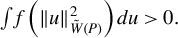 Thus, there exists a constant
$C_1>0$
 such that, for all sufficiently small c,

Therefore, for some constant
$C_2>0$
 ,
$I_c(P)\ge C_2 c^{(p-k)/2}.$
 Since
$k>p$
 , it follows that
$I_c(P)\to \infty $
 , and hence
$w_{1,c}\to 1$
 .
Finally, for any
$\varepsilon>0$
 ,

The first term converges to zero by Proposition 2, while the second converges to zero because
$1-w_{1,c}\to 0$
 . This proves the claim.
$\Box $

Proof of Proposition 5
Classic results in statistics, for example, Muirhead (Reference Muirhead1982, Chap. 1.5), imply the result for the case of a single regressor. For completeness, we prove the result for the general case. The confidence interval (7) corresponds to the set of values for
$v'\theta $
 where the test statistic

has absolute value less than
$t^*_{k-p,1-\frac {\beta }{2}}$
 . Hence, if we can show that (A.5) follows a
$t_{k-p}$
 distribution under all priors
$\pi $
 satisfying Assumptions 1 and 2, the result is immediate.
Note that (A.5) is equal to the t-statistic from regression (8) in the text:

where, again,
$M(P)=\tilde X(P)(\tilde X(P)'\tilde X(P))^{-1}\tilde X(P)'$
 . Specifically,
$\frac {\tilde {\eta }'(I-M(P))\tilde {\eta }}{k-p}$
 corresponds to the unbiased variance estimate, so the denominator
$\sqrt {\frac {\tilde {\eta }'(I-M(P))\tilde {\eta }}{k-p} \sigma _v^2(P)}$
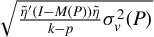 corresponds to the homoskedastic standard error. Note, moreover, that the t-statistic is scale-invariant in the error, so (A.6) is equal to

Lemma 2 implies that
$\frac {\tilde \eta }{\|\tilde \eta \|}$
 is uniformly distributed on the unit sphere under any prior
$\pi $
 satisfying Assumptions 1 and 2. However, this is exactly the distribution of
$\frac {Z}{\|Z\|}$
 for
$Z\sim N(0,I).$
 It follows that, under
$\pi ,$
 (A.6) has the same distribution as

where we have again used scale invariance of the t-statistic. However, the last expression is the t-statistic from the regression

which is well-known to be
$t_{k-p}$
 distributed, completing the proof.
$\Box $