


1 Introduction
If one fixes a Wang tileset, then the problem of generating a tiling of a plane is difficult in general. In the worst case, Hanf and Myers [Reference HanfHan74, Reference MyersMye74] showed the existence of tilesets that tile the plane, but for which no algorithm can produce any tiling. On the other end of the spectrum, certain tilesets admit a simple procedure that can generate any tiling of the plane, in which the choices of the tiles in each cell only require local interaction (we give an example in the next paragraphs).
In this article, we investigate the problem, given a fixed Wang tileset or a more general subshift, of generating all the tilings of the plane in a local way, that is, with a minimal amount of communication between the cells. Of course, one expects that only very few tilesets admit such local generation procedures. Our goal is to give precise definitions capturing this idea of local generation and then to settle whether each given tileset or subshift satisfies these definitions. Let us stress that our perspective is orthogonal to the viewpoints provided by computability and complexity theory, and that the locality of a procedure is a form of combinatorial rather than computational simplicity.
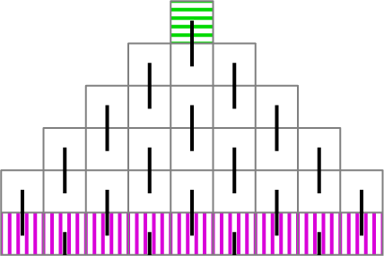
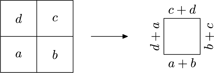
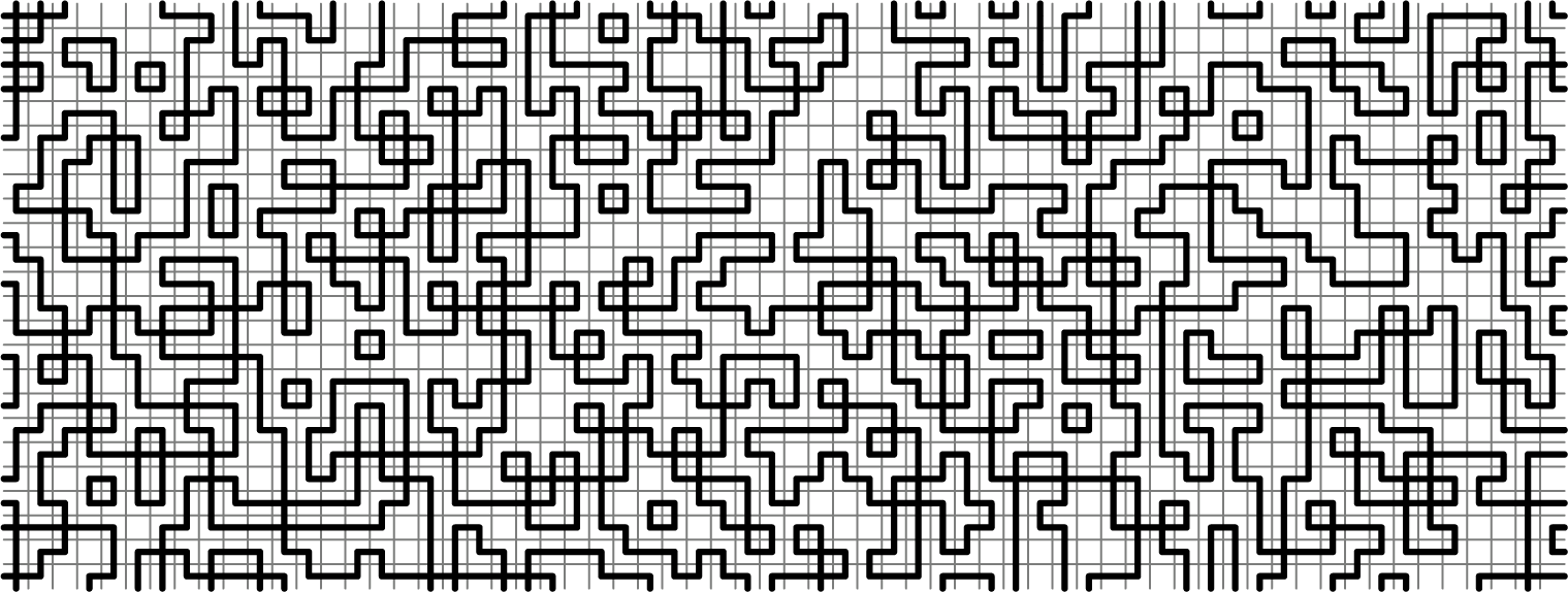
Let us start by illustrating a simple local generation procedure on a motivating example, which is the Wang tileset shown in Figure 1. It is the tileset with two colours (on the picture, an edge is either white or crossed by a black line) containing all the tiles having an even number of each colour.
A tileset admitting a local generation procedure.

There is a simple local way of generating any tiling of the plane. First, assign arbitrary bits to the points of the grid
 $\mathbb {Z}^2$
, then for each edge
 $(a,b)$
between two adjacent points, draw a black line crossing that edge if and only if the bits assigned to a and b differ. Intuitively, the bit assignment partitions
 $\mathbb {Z}^2$
into connected components on which the assignment is constant and the black lines are the boundaries between these regions. This construction is local in the sense that if two cells are not neighbours (horizontally, vertically or diagonally), then the choices of the tiles that are placed in those cells are made independently. The procedure that generates a tiling takes as input an arbitrary assignment of bits to the points of the grid, each cell then reads the bits assigned to its four corners and determines its tile. Note that this procedure enables adjacent cells to communicate in the sense that they share some input information. Similar procedures are used in computer graphics to generate textures in an efficient and local way [Reference LagaeLag09].
A first natural definition that would capture this generation procedure would be that the subshift is a factor of a fullshift, that is, the image of a fullshift by a so-called sliding block code [Reference Lind and MarcusLM95], which is a finite rule determining the output content of a cell from the input content of a neighbourhood of that cell. Indeed, the set of all possible assignments of bits is the fullshift
 $\{0,1\}^{\mathbb {Z}^2}$
and the function that converts this colour assignment to the assignment of tiles to the cells can be evaluated in a local way. Equivalently, a sliding block code is a continuous function that commutes with the shift and can be seen as cellular automata with possibly different input and output alphabets.
However, this tentative definition would be very restrictive in several ways:
-
• only nearby cells can communicate, that is, share input information;
-
• all the cells are required to have the same rule.
We will relax these restrictions in our definitions. However, there is an important feature that we want to keep:
-
• the content of each cell is determined by an input region whose size is uniformly bounded across the cells.
When this restriction is met, it gives rise to a procedure in which all the cells can determine their contents in parallel, reading a constant number of input symbols, so this procedure runs in constant parallel time.
We introduce two possible formalizations of the intuitive idea of local generation by defining two classes of subshifts
 $\mathscr {L}^0\subseteq \mathscr {L}^1$
. The class
 $\mathscr {L}^0$
is defined as the smallest class of subshifts containing certain basic subshifts (to be defined) including fullshifts, and closed under finite products and factors. The class
 $\mathscr {L}^1$
is based on the notion of narrow function which is a relaxation of sliding block codes, in which the content of each output cell is determined by the content of a finite region of input cells whose size is bounded, but whose shape is arbitrary. The definition of
 $\mathscr {L}^1$
is purely combinatorial in that it does not interact with the dynamical structure of the subshift. We never address the computability or complexity of the underlying procedures and only focus on some sort of combinatorial complexity.
We develop the theories of the classes
 $\mathscr {L}^0$
and
 $\mathscr {L}^1$
, identify two obstructions to being in these classes, and apply these techniques to a number of subshifts. We also show that one-dimensional subshifts of finite type (SFTs) all belong to
 $\mathscr {L}^0$
. It is not surprising as those subshifts are known to have many good properties. In particular, their configurations are nothing else than bi-infinite walks in a finite graph, which are intuitively easy to generate; the result shows that the class
 $\mathscr {L}^0$
is sufficiently rich to capture this intuition. In a forthcoming article [Reference Favereau and HoyrupFH24], we apply the techniques developed in this article to classify all the Wang tilesets made with bicolour tiles having an even number of each colour. We briefly summarize this classification at the end of this article.
The study of the class
 $\mathscr {L}^0$
is related to the problem of expressing a subshift as a factor of another subshift, which was investigated in [Reference Briceño, McGoff and PavlovBMP18, Reference BoyleBoy83, Reference Boyle, Pavlov and SchraudnerBPS10, Reference MarcusMar79], but our results are rather orthogonal.
The article is organized as follows. In §2, we present the definition of the two classes of subshifts
 $\mathscr {L}^0$
and
 $\mathscr {L}^1$
. In §3, we introduce the notions from symbolic dynamics that will play an important role in our analysis, recalling classical definitions and stating useful properties. In §4, we investigate several properties of our two classes. In §5, we develop a technique to prove that a subshift does not belong to
 $\mathscr {L}^0$
and apply it to a number of subshifts. We carry out an analogous development for
 $\mathscr {L}^1$
in §6, using different arguments. In §7, we identify several subshifts that belong to
 $\mathscr {L}^0$
, among which are the one-dimensional SFTs. In §8, we summarize the classification of the even bicolour tilesets. We end with §9 where we suggest future research directions. We also include an Appendix A, containing classical results that are used in the proofs.
2 Local generation
Let us first recall the minimal amount of definitions needed to introduce our notions of local generation.
2.1 Preliminaries
For
 $d\geq 1$
,
 $(\mathbb {Z}^d,+,0)$
is an abelian group. A
 $\mathbb {Z}^d$
-action on a set E is a homomorphism from
 $\mathbb {Z}^d$
to the group of bijections from E to E with the composition operation. We also say that E is a
 $\mathbb {Z}^d$
-set. The result of applying the image of
 $p\in \mathbb {Z}^d$
under the homomorphism to
 $e\in E$
is written as
 $p\cdot e\in E$
. A continuous
 $\mathbb {Z}^d$
-action on a topological space X is a homomorphism from
 $\mathbb {Z}^d$
to the group of homeomorphisms from X to X with the composition operation. We also say that X is a
 $\mathbb {Z}^d$
-space. A
 $\mathbb {Z}^d$
-space Y is a factor of a
 $\mathbb {Z}^d$
-space X if there exists a continuous surjective map
 $f:X\to Y$
that commutes with the actions:
 $p\cdot f(x)=f(p\cdot x)$
. f is called a factor map.
If A is a finite alphabet and E is countable, then
 $A^E$
is endowed with the Cantor topology, which is the product of the discrete topology on A. This makes
 $A^E$
a compact metrizable space. The shift action on
 $A^{\mathbb {Z}^d}$
is the continuous
 $\mathbb {Z}^d$
-action defined, for
 $p\in \mathbb {Z}^d$
and
 $x\in A^{\mathbb {Z}^d}$
, by
 $p\cdot x=y$
where
 $y(q)=x(p+q)$
. A
 $\mathbb {Z}^d$
-subshift is a compact set
 $X\subseteq A^{\mathbb {Z}^d}$
which is shift-invariant, that is, satisfies
 $\sigma ^p(X)=X$
for all
 $p\in \mathbb {Z}^d$
. A
 $\mathbb {Z}^d$
-fullshift is
 $A^{\mathbb {Z}^d}$
for some finite alphabet A.
2.2 The class
 $\mathscr {L}^0$

We start with the strongest notion of local generation. The definition is motivated by the following observations:
-
• certain particular subshifts have a generation procedure that is intuitively local;
-
• if two subshifts X and Y can be locally generated, then so is their product
$X\times Y$
(which is indeed a subshift), because the content of a cell is simply a pair whose components can be locally generated; -
• if a subshift X can be locally generated, then so is any factor Y of X. Indeed, if
$f:X\to Y$
is a factor map, then the value of
$f(x)_p$
is determined by the values of x in finitely many cells around p, which in turn can be locally generated.


We then define the class
 $\mathscr {L}^0$
as the smallest class of subshifts containing the basic subshifts from the first item, and that is closed under finite products and factors. We first need to choose basic subshifts to start with. We propose the following three families and explain why they can be considered as locally generated.
-
• Fullshifts
$A^{\mathbb {Z}^d}$
: the contents of the cells can be chosen independently of each other. -
• Periodic shifts: given a subgroup
$H\subseteq \mathbb {Z}^d$
, let
$X_H\subseteq A^{\mathbb {Z}^d}$
be the subshift containing all the H-periodic configurations, that is,
$x\in X_H$
if
$x(p+h)=x(p)$
for all
$p\in \mathbb {Z}^d$
and
$h\in H$
. First, an element of
$A^{\mathbb {Z}^d/H}$
can be generated by independent choices, and then the content of a cell
$p\in \mathbb {Z}^d$
is determined by the symbol assigned to its equivalence class in
$\mathbb {Z}^d/H$
. We will denote
$X_H$
by
$A^{\mathbb {Z}^d/H}$
. -
• Countable subshifts: the configurations of a countable subshift can be indexed by
$\mathbb {N}$
, so a configuration can be produced by first choosing a natural number n shared by all the cells and then all the cells determine their contents in parallel. All the cells have the same input information, namely n, which is therefore bounded across the cells (although the bound varies with the input n). We do not address the computability or complexity of this procedure (it was shown in [Reference Salo and TörmäST13] that countable subshifts can be very uncomputable).


Definition 2.1. (The class
$\mathscr {L}^0$
)

Let
 $d\geq 1$
. We define
 $\mathscr {L}^0_d$
as the smallest class of subshifts containing the
 $\mathbb {Z}^d$
-fullshifts, the periodic
 $\mathbb {Z}^d$
-shifts and the countable
 $\mathbb {Z}^d$
-subshifts, and which is closed under finite products and factors. Let
 $\mathscr {L}^0=\bigsqcup _{d\geq 1}\mathscr {L}^0_d$
.
First, subshifts in
 $\mathscr {L}^0$
can be presented in a simple form.
Proposition 2.2. (Canonical form)
One has
 $X\in \mathscr {L}^0$
if and only if X is a factor of a finite product of basic subshifts. Moreover, we can assume that this finite product is
 $$ \begin{align*} K\times A^{\mathbb{Z}^d}\times A^{\mathbb{Z}^d/H_1}\times \cdots\times A^{\mathbb{Z}^d/H_k}, \end{align*} $$
where K is countable, A is finite and
 $H_1,\ldots ,H_k$
are non-trivial subgroups of
 $\mathbb {Z}^d$
of ranks at most
 $d-1$
(and possibly
 $k=0$
).
Proof. We first show that every
 $X\in \mathscr {L}^0$
is a factor of a finite product of basic subshifts by induction on the finite tree describing the construction of X. If X is a basic subshift, then there is nothing to do. If
 $X=X_0\times X_1$
with
 $X_0,X_1\in \mathscr {L}^0$
, then by induction,
 $X_0=f_0(P_0)$
and
 $X_1=f_1(P_1)$
, where
 $f_0,f_1$
are factor maps and
 $P_0,P_1$
are finite products of basic subshifts. Therefore,
 $X=f(P_0\times P_1)$
, where
 $f(x_0,x_1)=(f_0(x_0),f_1(x_1))$
, and note that f is a factor map and
 $P_0\times P_1$
is a finite product of basic subshifts. If
 $X=f(Y)$
, where
 $Y\in \mathscr {L}^0$
and f is a factor map, then by induction,
 $Y=g(P)$
for some finite product P of basic subshifts and some factor map g, so
 $x=f\circ g(P)$
and
 $f\circ g$
is a factor map.
Finally, a finite product of countable subshifts is a countable subshift, a finite product of fullshifts is a fullshift, and one can replace all the involved alphabets by the largest one because if
 $A\subseteq B$
and
 $H\subseteq \mathbb {Z}^d$
, then
 $A^{\mathbb {Z}^d/H}$
is a factor of
 $B^{\mathbb {Z}^d/H}$
. If H is trivial, then
 $A^{\mathbb {Z}^d/H}$
is a fullshift. If H has rank d, then
 $A^{\mathbb {Z}^d/H}$
is finite and hence countable so it can be merged with K.
Note that the presence of a periodic shift
 $A^{\mathbb {Z}^d/H}$
in the canonical form intuitively allows output cells that differ by an element of H to ‘communicate’, in the sense that they share some amount of input information and can make their choices in tandem with each other.
It will be convenient to present a canonical form in a more condensed way, as follows.
Proposition 2.3. One has
 $X\in \mathscr {L}^0$
if and only if X is a factor of
 $K\times A^E$
, where K is a countable subshift, A is finite and E is a countable
 $\mathbb {Z}^d$
-set.
It is understood that
 $A^E$
is endowed with the
 $\mathbb {Z}^d$
-action
 $(u\cdot a)_p=a_{u\cdot p}$
for
 $a\in A^E$
, and that
 $K\times A^E$
is endowed with the product
 $\mathbb {Z}^d$
-action
 $u\cdot (k,a)=(u\cdot k,u\cdot a)$
.
Proof. If
 $X\in \mathscr {L}^0$
, then by Proposition 2.2, X is a factor of
 $K\times A^{\mathbb {Z}^d}\times A^{\mathbb {Z}^d/H_1}\times \cdots \times A^{\mathbb {Z}^d/H_k}=K\times A^E$
, where
 $E=\mathbb {Z}^d\sqcup \mathbb {Z}^d/H_1\sqcup \cdots \sqcup \mathbb {Z}^d/H_k$
endowed with the natural
 $\mathbb {Z}^d$
-action.
Conversely, if X is a factor of
 $K\times A^E$
for some countable
 $\mathbb {Z}^d$
-set E, then by the orbit-stabilizer theorem (Theorem A.3), one has
 $E=\bigsqcup _{i\in I}\mathbb {Z}^d/H_i$
, where I is countable and
 $H_i$
is a subgroup of
 $\mathbb {Z}^d$
. By compactness of
 $K\times A^E$
and continuity of f, there exists a finite set
 $R\subseteq E$
such that
 $f(k,x)_0$
is determined by the values of x on R. As f is a factor map, for any
 $p\in \mathbb {Z}^d$
,
 $f(k,x)_p$
is determined by the values of x on
 $p\cdot R=\{p\cdot e:e\in R\}$
. Therefore,
 $f(k,x)$
is determined by the values of x on the orbits of elements of R. As R is finite, there are finitely many such orbits, so X is a factor of
 $K\times A^{E'}$
, where
 $E'$
is a finite disjoint union of quotients of
 $\mathbb {Z}^d$
, so
 $A^{E'}$
is a finite product of
 $A^{\mathbb {Z}^d/H_i}$
.
Example 2.4. (Cellular automaton)
A cellular automaton is a continuous function
 $f:A^{\mathbb {Z}^d}\to A^{\mathbb {Z}^d}$
which commutes with the shift action, so its image is a factor of a fullshift and always belongs to
 $\mathscr {L}^0$
.
2.3 The class
$\mathscr {L}^1$

We present the second definition of local generation, which is a relaxation of the first one in which we forget the dynamical aspects of subshifts. We first need the following notions to formulate the definition of
 $\mathscr {L}^1$
.
Let
 $E,F$
be countable sets,
 $A,B$
be finite alphabets and
 $f:A^E\to B^F$
be continuous. The following notion is a restriction on the continuity of f, in which each output position has a narrow view on the input of f.
Definition 2.5. (Narrow function)
We say that
 $q\in F$
is determined by
 $R\subseteq E$
if for all inputs
 $x,y\in A^E$
that coincide on R,
 $f(x)$
and
 $f(y)$
coincide at position q.
Let
 $r\in \mathbb {N}$
. The function
 $f:A^E\to B^F$
is r-narrow if each
 $q\in F$
is determined by a region of size at most r. We say that f is narrow if f is r-narrow for some r.
Note that a function is
 $0$
-narrow if and only if it is constant. The identity
 $f:A^E\to A^E$
is
 $1$
-narrow. Every factor map is narrow. The composition of two narrow functions is narrow.
Example 2.6. (Non-uniform cellular automaton)
A non-uniform cellular automaton [Reference Dennunzio, Formenti and ProvillardDFP12] is a continuous function
 $f:A^{\mathbb {Z}^d}\to A^{\mathbb {Z}^d}$
such that each
 $q\in \mathbb {Z}^d$
is determined by
 $\mathcal {N}(q,r)=\{p\in \mathbb {Z}^d:d(p,q)\leq r\}$
for some
 $r\in \mathbb {N}$
(the metric d is defined by
 $d(p,q)=\max _i |p_i-q_i|$
, where
 $p_i,q_i$
are the coordinates of
 $p,q$
, respectively). The size of
 $\mathcal {N}(q,r)$
is constant so f is narrow.
We come to the second notion of local generation. Let
 $\Sigma $
be finite and F be countable.
Definition 2.7. (The class
$\mathscr {L}^1$
)

A compact set
 $X\subseteq \Sigma ^F$
belongs to
 $\mathscr {L}^1$
if it is a countable union of images of narrow functions, that is,
 $X=\bigcup _{n\in \mathbb {N}} X_n$
, where
 $X_n=\mathrm {im}(f_n)$
and
 $f_n:A_n^{\mathbb {N}}\to X$
is
 $r_n$
-narrow.
Note that
 $\mathbb {N}$
can be replaced by any countable set. We will mostly consider the case when
 $F=\mathbb {Z}^d$
and X is a
 $\mathbb {Z}^d$
-subshift, but the definition makes sense more generally.
Finally, this notion of local generation is indeed a relaxation of the previous one.
Proposition 2.8. One has
 $\mathscr {L}^0\subseteq \mathscr {L}^1$
.
Proof. Let
 $X\in \mathscr {L}^0$
and let
 $f:K\times A^E\to X$
be a factor map given by Proposition 2.3. For each
 $k\in K$
, let
 $f_k:A^E\to X$
send a to
 $f(k,a)$
. As f is narrow, each
 $f_k$
is narrow so
 $X=\bigcup _{k\in K}\mathrm {im}(f_k)$
belongs to
 $\mathscr {L}^1$
, as K is countable.
The following notion will be useful to analyse narrow functions.
Proposition 2.9. (Input window)
Let
 $f:A^E\to B^F$
be continuous. For each
 $q\in F$
, there is a minimal subset of E that determines q. It is denoted by
 $\mathcal {W}_f(q)$
and is called the input window of q.
Proof. Let
 $\mathcal {W}_f(q)$
be the intersection of all the sets that determine q. We show that
 $\mathcal {W}_f(q)$
determines q. Let
 $x,y\in A^E$
coincide on
 $\mathcal {W}_f(q)$
. As f is continuous, there is a finite set R that determines q, so
 $\mathcal {W}_f(q)\subseteq R$
. Let
 $R\setminus \mathcal {W}_f(q)=\{r_1,\ldots ,r_n\}$
. For each
 $i\leq n$
, there exists
 $R_i$
that determines q and such that
 $r_i\notin R_i$
. We inductively define
 $x_0,x_1,\ldots ,x_n$
as follows. Let
 $x_0=x$
and for
 $i<n$
, let
 $x_{i+1}$
coincide with
 $x_i$
everywhere except possibly at
 $r_i$
, where it takes the same value as y. As
 $x_{i+1}$
and
 $x_i$
coincide on
 $R_i$
which determines q,
 $f(x_{i+1})$
and
 $f(x_i)$
coincide at q. As
 $x_n$
coincides with y on R which determines q,
 $f(x_n)$
and
 $f(y)$
coincide at q. As a result,
 $f(x)$
and
 $f(y)$
coincide at q, so
 $\mathcal {W}_f(q)$
indeed determines q.
One should think of each output position
 $q\in F$
as observing the input of f through its input window
 $\mathcal {W}_f(q)$
and then choosing its content according to what it sees. A function f is r-narrow if
 $|\mathcal {W}_f(q)|\leq r$
for all q.
2.3.1 Relevance of the definition
We now discuss why a compact set in
 $\mathscr {L}^1$
always admits a generation procedure which is in a sense local.
Let
 $X\in \mathscr {L}^1$
, that is,
 $X=\bigcup _{n\in \mathbb {N}} X_n$
, where
 $X_n$
is the image of some
 $r_n$
-narrow function
 $f_n:A_n^{\mathbb {N}}\to \Sigma ^{\mathbb {Z}^d}$
. The procedure producing a configuration
 $x\in X$
runs as follows:
-
• choose a number
$n\in \mathbb {N}$
and an arbitrary sequence of symbols
$a\in A^{\mathbb {N}}_n$
; -
• for each cell
$p\in \mathbb {Z}^d$
, read the values of a in at most
$r_n$
positions, determine the value of
$f_n(a)$
at position p and fill p with that value.


Therefore, each cell has its own procedure, which takes some amount of input information and outputs its content. The important properties of this procedure are that for each input
 $(n,a)$
, the size of the information used by the cells is bounded across the cells (although the bound can depend on n) and all the cells run their procedures in parallel with no explicit communication. Some amount of communication is implicitly made possible as the cells share limited pieces of input information, via the number n and the overlaps between the windows of the cells, and again this information is bounded across the cells (and the bound can depend on n).
Again, we do not address the computability or complexity of computing the finite input window of each position and applying the rule that determines the output, and our results only focus on the ‘combinatorial’ complexity of subshifts. In practice, the class
 $\mathscr {L}^1$
will mainly be used to prove that particular subshifts do not belong to that class, which a fortiori prevents the existence of efficiently computable windows and rules. Conversely, for every particular subshift
 $X\in \mathscr {L}^1$
considered in this article, the windows and rules will be explicit and efficiently computable.
3 Symbolic dynamics
We recall the classical vocabulary associated to subshifts.
3.1 Definitions
Let
 $d\geq 1$
and
 $\Sigma $
be a finite alphabet.
We endow
 $\mathbb {Z}^d$
with the metric
 $d(p,q)=\max _i|p_i-q_i|$
, where
 $p=(p_1,\ldots ,p_d)$
and
 $q=(q_1,\ldots ,q_d)$
. For
 $F\subseteq \mathbb {Z}^d$
,
 $\mathop {\mathrm {diam}}(F)=\max _{p,q\in F}d(p,q)$
, which is
 $\infty $
if F is infinite. For
 $F,G\subseteq \mathbb {Z}^d$
,
 $d(F,G)=\min _{p\in F,q\in G}d(p,q)$
. We will often consider the cubes
 $S_n=[0,n-1]^d$
and
 $Q_n=[-n,n]^d$
for
 $n\in \mathbb {N}$
.
Let
 $F\subseteq \mathbb {Z}^d$
be any set. An F-pattern is an element
 $\pi \in \Sigma ^F$
. A pattern is an F-pattern for some F, which is called the domain of
 $\pi $
and is denoted by
 $\mathrm {dom}(\pi )$
. A pattern
 $\pi '$
extends a pattern
 $\pi $
if
 $\mathrm {dom}(\pi )\subseteq \mathrm {dom}(\pi ')$
and
 $\pi '(p)=\pi (p)$
for all
 $p\in \mathrm {dom}(\pi )$
. A finite pattern is an F-pattern for some finite
 $F\subseteq \mathbb {Z}^d$
. If
 $\pi ,\pi '$
are patterns with disjoint domains
 $F,F'$
, respectively, then
 $\pi \cup \pi '$
is the pattern with domain
 $F\cup F'$
extending
 $\pi $
and
 $\pi '$
. A configuration is an element
 $x\in \Sigma ^{\mathbb {Z}^d}$
.
If
 $\pi $
is a pattern, then
 $[\pi ]$
is the set of configurations extending
 $\pi $
. The set
 $\Sigma ^{\mathbb {Z}^d}$
is endowed with the topology generated by the sets
 $[\pi ]$
, where
 $\pi $
is a finite pattern. As already mentioned, the space
 $\Sigma ^{\mathbb {Z}^d}$
is endowed with the shift action, which is the continuous
 $\mathbb {Z}^d$
-action
 $p\cdot x=y$
, where
 $y(q)=x(p+q)$
. We will often write
 $\sigma ^p(x):=p\cdot x$
. The shift also acts on patterns: if
 $\pi $
is an F-pattern, then
 $\sigma ^p(\pi )$
is the
 $F'$
-pattern
 $\pi '$
, where
 $F'=F-p$
and
 $\pi '(q)=\pi (p+q)$
for
 $q\in F'$
. If
 $p\in \mathbb {Z}^d$
and x is a configuration, then we say that a pattern
 $\pi $
appears at position p in x if
 $\sigma ^p(x)$
extends
 $\pi $
.
A subshift is a closed subset X of
 $\Sigma ^{\mathbb {Z}^d}$
which is shift-invariant, that is, satisfies
 $\sigma ^p(X)=X$
for all
 $p\in \mathbb {Z}^d$
. We fix a subshift
 $X\subseteq \Sigma ^{\mathbb {Z}^d}$
. All the subsequent notions are relative to X, but we do not mention X which will always be clear from the context. A valid configuration is an element
 $x\in X$
. A valid pattern is a pattern appearing in some valid configuration, at any position or equivalently at the origin. Two disjoint regions
 $F,G\subseteq \mathbb {Z}^d$
are independent if for every valid F-pattern
 $\pi $
and every valid G-pattern
 $\pi '$
,
 $\pi \cup \pi '$
is valid.
A subshift of finite type (SFT) is the subshift induced by a finite set P of finite patterns, called forbidden patterns and defined as the set of configurations in which no
 $\pi \in P$
appears. Let C be a finite set of colours. A Wang tile over C associates to each edge of the unit square a colour in C. A Wang tileset over C is a set T of Wang tiles over C. It induces a
 $\mathbb {Z}^2$
-subshift of finite type
 $X_T\subseteq T^{\mathbb {Z}^2}$
which is the set of configurations in which neighbour cells have the same colour on their common edge.
3.2 Dynamical properties
We recall classical dynamical properties of subshifts that can be found in [Reference FurstenbergFur67] or [Reference de VriesdV13].
Definition 3.1. A subshift
 $X\subseteq \Sigma ^{\mathbb {Z}^d}$
is transitive if for every pair of valid finite patterns
 $\pi ,\pi '$
, there exists
 $p\in \mathbb {Z}^d$
such that
 $\pi \cup \sigma ^p(\pi ')$
is a valid pattern; in other words,
 $\pi $
and
 $\pi '$
appear in a common configuration.
A subshift
 $X\subseteq \Sigma ^{\mathbb {Z}^d}$
is strongly irreducible if there exists
 $n\in \mathbb {N}$
such that all regions
 $F,G\subseteq \mathbb {Z}^d$
satisfying
 $d(F,G)\geq n$
are independent.
A subshift
 $X\subseteq \Sigma ^{\mathbb {Z}^d}$
is mixing if for every
 $m\in \mathbb {N}$
, there exists
 $n\in \mathbb {N}$
such that all regions
 $F,G\subseteq \mathbb {Z}^d$
satisfying
 $\mathop {\mathrm {diam}}(F)\leq m,\mathop {\mathrm {diam}}(G)\leq m$
and
 $d(F,G)\geq n$
are independent.
A subshift
 $X\subseteq \Sigma ^{\mathbb {Z}^d}$
is weakly mixing if
 $X\times X$
is transitive.
Transitive systems are called ergodic in [Reference FurstenbergFur67] and are also referred to as irreducible in the literature. In the definitions of transitivity, weak mixing and mixing, one can equivalently replace finite regions by cubes
 $Q_m$
. However, the version of strong irreducibility restricted to cubes is strictly weaker in general and is called block-gluing. One has the following chain of implications:
strongly irreducible
 $\implies $
mixing
 $\implies $
weakly mixing
 $\implies $
transitive.
Strong irreducibility is a simple necessary condition for a subshift to be a factor of a fullshift.
The notion of weak mixing will be important in this article. Its meaning might not be clear at first, but the characterization given condition (3) in the next proposition is much more intuitive, easier to work with and is more apparently a relaxation of the mixing property. A part of this result was proved by Furstenberg [Reference FurstenbergFur67] in the context of continuous
 $\mathbb {Z}$
-actions.
Proposition 3.2. (Characterizations of weak mixing)
For a subshift
 $X\subseteq \Sigma ^{\mathbb {Z}^d}$
, the following conditions are equivalent:
-
(1) X is weakly mixing;
-
(2) for each
$k\geq 1$
,
$X^k$
is transitive; -
(3) for every
$n\in \mathbb {N}$
, there exists
$p\in \mathbb {Z}^d$
such that
$Q_n$
and
$p+Q_n$
are independent; -
(4) for every
$n\in \mathbb {N}$
and every valid
$Q_n$
-pattern
$\pi $
, there exists
$p\in \mathbb {Z}^d$
such that for every valid
$Q_n$
-pattern
$\pi '$
,
$\pi \cup \sigma ^p(\pi ')$
is valid.


The result still holds if one replaces the quantification over n by a quantification over the finite regions
 $F\subseteq \mathbb {Z}^d$
(and the
 $Q_n$
-patterns by F-patterns).
Proof.
 $(1)\Rightarrow (2).$
Let
 $n\in \mathbb {N}$
and let
 $\pi _1,\ldots ,\pi _k$
and
 $\pi ^{\prime }_1,\ldots ,\pi ^{\prime }_k$
be valid
 $Q_n$
-patterns. Our goal is to prove the existence of
 $p\in \mathbb {Z}^d$
such that each
 $\pi _i\cup \sigma ^p(\pi ^{\prime }_i)$
is valid. By induction on
 $i\leq k$
, we show the existence of
 $p_1,\ldots ,p_i$
such that
 $\mu _i=\bigcup _{j\leq i}\sigma ^{p_j}(\pi _j)$
and
 $\mu ^{\prime }_j=\bigcup _{j\leq i}\sigma ^{p_j}(\pi ^{\prime }_j)$
are both valid. Start with
 $p_1=0$
, and note that
 $\pi _1$
and
 $\pi ^{\prime }_1$
are valid by assumption. For
 $i<k$
, assume that
 $p_1,\ldots ,p_{i}$
have been defined. As
 $X\times X$
is transitive, there exists
 $p_{i+1}\in \mathbb {Z}^d$
such that
 $\mu _i\cup \sigma ^{p_{i+1}}(\pi _{i+1})$
and
 $\mu ^{\prime }_i\cup \sigma ^{p_{i+1}}(\pi ^{\prime }_{i+1})$
are valid, which proves the induction step. Finally, as X is transitive, there exists p such that
 $\mu _k\cup \sigma ^p(\mu ^{\prime }_k)$
is valid. Observe that this pattern contains each
 $\sigma ^{p_i}(\pi _i\cup \sigma ^p(\pi ^{\prime }_i))$
, so each
 $p_i\cup \sigma ^p(\pi ^{\prime }_i)$
is valid.
 $(2)\Rightarrow (3).$
Let
 $n\in \mathbb {N}$
. Let
 $\{\pi _1,\ldots ,\pi _m\}$
be the set of valid
 $Q_n$
-patterns and
 $k=m^2$
. The two following patterns are valid in
 $X^k$
:
 $$ \begin{align*} \pi&=(\pi_1,\ldots,\pi_1,\pi_2,\ldots,\pi_2,\ldots,\pi_m,\ldots,\pi_m);\\ \pi'&=(\pi_1,\ldots,\pi_m,\pi_1,\ldots,\pi_m,\ldots,\pi_1,\ldots,\pi_m). \end{align*} $$
As
 $X^k$
is transitive, there exists
 $p\in \mathbb {Z}^d$
such that
 $\pi \cup \sigma ^p(\pi ')$
is valid in
 $X^k$
. It implies that for all
 $i,j\leq m$
,
 $\pi _i\cup \sigma ^p(\pi _j)$
is valid in X. As a result,
 $Q_n$
and
 $p+Q_n$
are independent.
 $(3)\Rightarrow (4).$
Observe that condition (3) is obtained from condition (4) by exchanging the quantifiers over p and
 $\pi $
, so condition (3) is indeed stronger than condition (4). Let us prove it more precisely. If
 $n\in \mathbb {N}$
and
 $\pi $
is a valid
 $Q_n$
-pattern, then let
 $p\in \mathbb {Z}^d$
be given by condition (3) applied to n. As
 $Q_n$
and
 $p+Q_n$
are independent, for every
 $Q_n$
-pattern
 $\pi '$
,
 $\pi \cup \sigma ^p(\pi ')$
is valid.
 $(4)\Rightarrow (1).$
Let
 $n\in \mathbb {N}$
and
 $\pi _1,\pi ^{\prime }_1,\pi _2,\pi ^{\prime }_2$
be valid
 $Q_n$
-patterns. Our goal is to find
 $q\in \mathbb {Z}^d$
such that both
 $\pi _1\cup \sigma ^q(\pi ^{\prime }_1)$
and
 $\pi _2\cup \sigma ^q(\pi ^{\prime }_2)$
are valid patterns. Applying condition (4) to n and
 $\pi _1$
, there exists
 $p\in \mathbb {Z}^d$
such that
 $\pi _1\cup \sigma ^p(\pi _2)$
is valid. Let
 $m\in \mathbb {N}$
be such that
 $Q_m$
contains
 $Q_n\cup (p+Q_n)$
and
 $\pi $
be a valid
 $Q_m$
-pattern extending
 $\pi _1\cup \sigma ^p(\pi _2)$
. Applying again condition (4) to m and
 $\pi $
gives some
 $q\in \mathbb {Z}^d$
. Let
 $\pi ^{\prime \prime }_1$
and
 $\pi ^{\prime \prime }_2$
be valid extensions on
 $Q_m$
of
 $\pi ^{\prime }_1$
and
 $\sigma ^p(\pi ^{\prime }_2)$
, respectively. By choice of q,
 $\pi \cup \sigma ^q(\pi ^{\prime \prime }_1)$
and
 $\pi \cup \sigma ^q(\pi ^{\prime \prime }_2)$
are valid. Finally, observe that
 $\pi \cup \sigma ^q(\pi ^{\prime \prime }_1)$
extends
 $\pi _1\cup \sigma ^q(\pi ^{\prime }_1)$
and
 $\pi \cup \sigma ^q(\pi ^{\prime \prime }_2)$
extends
 $\sigma ^p(\pi _2\cup \sigma ^q(\pi ^{\prime }_2))$
. As a result,
 $\pi _1\cup \sigma ^q(\pi ^{\prime }_1)$
and
 $\pi _2\cup \sigma ^q(\pi ^{\prime }_2)$
are valid.
To prove mixing properties, it is often convenient to consider regions having certain prescribed shapes.
Proposition 3.3. Let
 $\mathcal {F}$
be a family of finite subsets of
 $\mathbb {Z}^d$
such that every
 $Q_m$
is contained, up to translation, in some element of
 $\mathcal {F}$
.
A
 $\mathbb {Z}^d$
-subshift is mixing if and only if for every
 $F\in \mathcal {F}$
, there exists
 $n\in \mathbb {N}$
such that for every
 $p\in \mathbb {Z}^d$
satisfying
 $|p|\geq n$
, F and
 $p+F$
are independent.
Proof. Assume the property, let
 $m\in \mathbb {N}$
and let
 $H\in \mathcal {F}$
contain
 $h+Q_m$
for some
 $h\in \mathbb {Z}^d$
. Applying the property to H yields some n. Let
 $F,G$
have diameters at most m and satisfy
 $d(F,G)\geq n$
. Choose any
 $p\in F,q\in G$
and note that
 $d(p,q)\geq n$
. One has
 $F\subseteq p+Q_m\subseteq q-h+H$
and
 $G\subseteq q+Q_m\subseteq q-h+H$
. As
 $|(p-h)-(q-h)|=d(p,q)\geq~n$
,
 $p-h+H$
and
 $q-h+H$
are independent, so F and G are independent as well.
Conversely, assume that X is mixing, let
 $F\in \mathcal {F}$
and
 $m=\mathop {\mathrm {diam}}(F)$
. The mixing property yields some n. Let
 $n'=n+m$
and
 $|p|\geq n'$
. The regions F and
 $p+F$
have diameter m and
 $d(F,p+F)\geq |p|-\mathop {\mathrm {diam}}(F)\geq n$
, so F and
 $p+F$
are independent.
3.3 Weak factors and weak conjugacies
Usually, two
 $\mathbb {Z}^d$
-subshifts X and Y are considered equivalent when they are conjugate, which means that there exists a homeomorphism
 $f:X\to Y$
that commutes with the shift actions:
 $\sigma ^u\circ f=f\circ \sigma ^u$
for all
 $u\in \mathbb {Z}^d$
.
We will consider more flexible notions of factor and conjugacy, which allow one to move the group elements by a homomorphism, and are the natural notions of homomorphisms and isomorphisms in the category of continuous group actions, when the group is not fixed.
The main interest of these notions is that the classes
 $\mathscr {L}^0$
and
 $\mathscr {L}^1$
are preserved by taking weak factors, as we will show in the next section.
Definition 3.4. Let X be a
 $\mathbb {Z}^d$
-subshift and Y a
 $\mathbb {Z}^e$
-subshift. We say that Y is a weak factor of X if there exists a continuous surjective function
 $f:X\to Y$
and a homomorphism
 $\varphi :\mathbb {Z}^e\to \mathbb {Z}^d$
such that
 $$ \begin{align*} \sigma^p\circ f=f\circ \sigma^{\varphi(p)} \end{align*} $$
for all
 $p\in \mathbb {Z}^e$
.
Two subshifts
 $X,Y$
are weakly conjugate if moreover f is a homeomorphism and
 $\varphi $
an isomorphism (which is possible only when
 $d=e$
).
Note that a weak factor (respectively weak conjugacy) map
 $f:X\to Y$
can be seen as a factor (respectively conjugacy) map
 $f':X'\to Y$
, where
 $X'$
is X endowed with the
 $\mathbb {Z}^e$
-action
 $p\star x:=\varphi (p)\cdot x$
.
The Curtis–Hedlund–Lyndon theorem [Reference Lind and MarcusLM95, Theorem 6.2.9], stating that factor maps are equivalent to sliding block codes, immediately extends to weak factor maps.
Proposition 3.5. (Curtis–Hedlund–Lyndon theorem)
Let
 $\varphi :\mathbb {Z}^e\to \mathbb {Z}^d$
be a group homomorphism and
 $f:A^{\mathbb {Z}^d}\to B^{\mathbb {Z}^e}$
be a function. The following conditions are equivalent:
-
• f is continuous and satisfies
$\sigma ^p\circ f=f\circ \sigma ^{\varphi (p)}$
; -
• there exists
$N\geq 0$
and a function
$\rho :Q_N\to B$
, where
$Q_N=[-N,N]^d$
, such that
$f(x)_p=\rho (x|_{\varphi (p)+Q_N})$
.


We will call the function
 $\rho $
a rule. When
 $d=e$
and
 $\varphi $
is the identity, we are back to the notion of sliding block code.
Proof. The usual proof when
 $\varphi $
is the identity extends immediately as follows.
Assume the first conditions. As f is continuous, there exist N and
 $\rho $
such that
 $f(x)_0\kern1.3pt{=}\kern1.3pt\rho (x|_{Q_N})$
. One has
 $f(x)_p\kern1.3pt{=}\kern1.3pt(\sigma ^p\circ f(x))_0\kern1.3pt{=}\kern1.3pt(f(\sigma ^{\varphi (p)}(x))_0\kern1.3pt{=}\kern1.3pt\rho (\sigma ^{\varphi (p)}(x)|_{Q_N})=\rho (x|_{\varphi (p)+Q_N})$
.
Conversely, if f is given by N and
 $\rho $
, then f is continuous and
 $(\sigma ^q\circ f(x))_p=f(x)_{p+q}=\rho (x|_{\varphi (p)+\varphi (q)+Q_N})=\rho (\sigma ^{\varphi (q)}(x)|_{\varphi (p)+Q_N})=f(\sigma ^{\varphi (q)}(x))_p$
, so
 $\sigma ^q\circ f=f\circ \sigma ^{\varphi (q)}$
.
Let us illustrate the notions of weak factor and weak conjugacy on several examples.
Example 3.6. (Fullshifts of different dimensions)
If
 $d>e$
, then the fullshift
 $X_e:=\Sigma ^{\mathbb {Z}^e}$
is a weak factor of the fullshift
 $X_d:=\Sigma ^{\mathbb {Z}^d}$
. Let
 $\varphi :\mathbb {Z}^e\to \mathbb {Z}^d$
be any injective homomorphism and let
 $f:X_d\to X_e$
be defined by
 $f(x)=x\circ \varphi $
. One can check that
 $\sigma ^p\circ f=f\circ \sigma ^{\varphi (p)}$
and f is surjective because for every
 $y\in X_e$
, one can build a pre-image
 $x\in X_d$
by filling the positions in
 $\mathrm {im}(\varphi )$
(without any conflict as
 $\varphi $
is injective) and filling the rest arbitrarily.
However,
 $X_d$
is not a weak factor of
 $X_e$
. Indeed, if
 $f:X_e\to X_d$
is a weak factor map via a homomorphism
 $\varphi :\mathbb {Z}^d\to \mathbb {Z}^e$
, then
 $\varphi $
is non-injective and if
 $p\in \ker \varphi $
, then
 $f(X_e)$
only contains p-periodic configurations, as
 $\sigma ^p\circ f=F\circ \sigma ^{\varphi (p)}=f$
.
Example 3.7. (Geometric transformation)
Let
 $\varphi :\mathbb {Z}^d\to \mathbb {Z}^d$
be an isomorphism. It induces a homeomorphism
 $f:\Sigma ^{\mathbb {Z}^d}\to \Sigma ^{\mathbb {Z}^d}$
defined by
 $f(x)=x\circ \varphi $
. If
 $X\subseteq \Sigma ^{\mathbb {Z}^d}$
is a subshift, then
 $f(X)$
is also a subshift. It is usually not conjugate to X, but it is weakly conjugate because again,
 $\sigma ^p\circ f=f\circ \sigma ^{\varphi (p)}$
for all
 $p\in \mathbb {Z}^d$
.
For instance, a
 $\mathbb {Z}^2$
-subshift can be reflected across an axis, or rotated by
 $90$
degrees, yielding a weakly conjugate subshift.
Example 3.8. (Higher power presentation)
Let
 $X\subseteq \Sigma ^{\mathbb {Z}^d}$
be a subshift,
 $a=(a_1,\ldots , a_d)\in \mathbb {Z}^d$
have positive coordinates and
 $R_a=[0,a_1-1]\times \cdots \times [0,a_d-1]$
. The a-higher power presentation of X is the subshift
 $[X]_a\subseteq \Gamma ^{\mathbb {Z}^d}$
, where
 $\Gamma =\Sigma ^{R_a}$
, obtained by dividing
 $\mathbb {Z}^d$
into a regular grid of copies of the rectangle
 $R_a$
and seeing each pattern in such a rectangle as a symbol in the alphabet
 $\Gamma $
(it can be found in [Reference Lind and MarcusLM95, Definition 1.4.4] in the one-dimensional case). More formally,
 $[X]_a$
is the image of X by the function
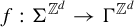 $f:\Sigma ^{\mathbb {Z}^d}\to \Gamma ^{\mathbb {Z}^d}$
defined by
 $f(x)=y$
, where
 $y(p)$
is the
 $R_a$
-pattern appearing at position
 $ap=(a_1p_1,\ldots ,a_dp_d)$
in x.
One has
 $\sigma ^p\circ f=f\circ \sigma ^{ap}$
, so
 $[X]_a$
is a weak factor of X via the homomorphism
 $\varphi (p)=ap$
.
Example 3.9. (Fullshifts on different alphabets)
Let
 $X=\Sigma ^{\mathbb {Z}^d}$
and
 $Y=\Gamma ^{\mathbb {Z}^d}$
be
 $\mathbb {Z}^d$
-fullshifts, with
 $|\Sigma |<|\Gamma |$
. First, X is a factor of Y: fix some surjective function
 $\Gamma \to \Sigma $
and extend it from Y to X. Conversely, Y is not a factor of X because the entropy of Y is
 $h(Y)=\log |\Gamma |$
, which is strictly larger than the entropy of X,
 $h(X)=\log |\Sigma |$
(see [Reference Lind and MarcusLM95]). However, Y is a weak factor of X. Indeed, let
 $n\in \mathbb {N}$
be such that
 $|\Sigma ^{n^d}|\geq |\Gamma |$
and
 $a=(n,\ldots ,n)\in \mathbb {Z}^d$
. The a-higher power presentation
 $[X]_a$
is the fullshift on the alphabet
 $\Sigma ^{n^d}$
so Y is a factor of
 $[X]_a$
, which is a weak factor of X (see Example 3.8), so Y is a weak factor of X.
In contrast to factors, weak factors do not preserve most of the dynamical properties, except the mixing property in some cases, as stated in the next result.
Proposition 3.10. Let X be a mixing subshift. If a subshift Y is a weak factor of X, then Y satisfies at least one of the two following properties:
-
• Y is periodic in the sense that there exists
$p\neq 0$
such that
$\sigma ^p(y)=y$
for all
$y\in Y$
; -
• or Y is mixing.


Proof. Let
 $f:X\to Y$
be a weak factor map via
 $\varphi :\mathbb {Z}^e\to \mathbb {Z}^d$
. If
 $\varphi $
is not injective, then let
 $p\in \ker (\varphi )$
be non-zero. One has
 $\sigma ^p\circ f=f\circ \sigma ^{\varphi (p)}=f$
, so
 $\sigma ^p(y)=y$
for all
 $y\in Y$
.
Now, assume that
 $\varphi $
is injective. Let
 $N\geq 0$
and
 $\rho $
be given by Proposition 3.5, satisfying
 $f(x)_p=\rho (x|_{\varphi (q)+Q_N})$
. Let
 $m\in \mathbb {N}$
, let
 $m'=\mathop {\mathrm {diam}}\varphi ([0,m]^e)+2N$
, let
 $n'$
be associated to
 $m'$
using the mixing property of X, and n be such that if
 $|p|\geq n$
, then
 $\varphi (p)\geq n'+2N$
. Such an n exists as
 $\varphi $
is injective. Let
 $F,G\subseteq \mathbb {Z}^e$
be two regions of diameters at most m and at distance at least n from each other. One has
 $\mathcal {W}_f(F)\subseteq \varphi (F)+Q_N$
and
 $\mathcal {W}_f(G)\subseteq \varphi (G)+Q_N$
, so
 $\mathcal {W}_f(F)$
and
 $\mathcal {W}_f(G)$
have diameters at most
 $m'$
. Moreover,
 $d(F,G)\geq n$
implies that
 $d(\varphi (F),\varphi (G))\geq n'+2N$
, so
 $d(\mathcal {W}_f(F),\mathcal {W}_f(G))\geq n'$
. By the mixing property of X,
 $\mathcal {W}_f(F)$
and
 $\mathcal {W}_f(G)$
are independent, so F and G are independent as well.
4 Properties of the classes
$\mathscr {L}^0$
and
$\mathscr {L}^1$


We investigate general properties of the classes.
First, belonging to
 $\mathscr {L}^0$
implies the existence of strongly periodic configurations. A configuration
 $x\in \Sigma ^{\mathbb {Z}^d}$
is strongly periodic if its orbit
 $\{\sigma ^p(x):p\in \mathbb {Z}^d\}$
is finite; equivalently, if there exists
 $k\in \mathbb {N}\setminus \{0\}$
such that
 $\sigma ^{kp}(x)=x$
for all
 $p\in \mathbb {Z}^d$
. It is known that every countable subshift contains a strongly periodic configuration [Reference Ballier, Durand, Jeandel, Albers and WeilBDJ08, Reference DolbilinDol95] (indeed, any configuration of maximal Cantor–Bendixson rank is strongly periodic).
Proposition 4.1. Every subshift in
 $\mathscr {L}^0$
has strongly periodic configurations.
Proof. Let
 $f:K\times A^E\to X$
be a factor map. As K is countable, it contains a strongly periodic configuration x. Let a be a constant sequence in
 $A^e$
. The orbit of
 $(x,a)$
is finite, so the orbit of
 $y=f(x,a)$
is finite as well.
The next result investigates simple closure properties of narrow functions. It will only be used in §6.3.2 and can be skipped at first reading.
Proposition 4.2. Let
 $\Sigma $
be a finite alphabet,
 $d\geq 1$
and
 $X,Y\subseteq \Sigma ^{\mathbb {Z}^d}$
be compact.
-
• If
$X,Y$
are images of narrow functions, then so is
$X\cup Y$
. -
• If X is the image of a narrow function and
$\pi $
is a finite pattern, then
$X\cap [\pi ]$
is the image of a narrow function. -
• If
$X\in \mathscr {L}^1$
, then there exists a finite pattern
$\pi $
such that
$X\cap [\pi ]$
is the image of a narrow function.


Proof. Let
 $f:A^{\mathbb {N}}\to X$
and
 $g:A^{\mathbb {N}}\to Y$
be surjective narrow functions with
 $|A|\geq 2$
(we can indeed assume that they start from the same alphabet). Let
 $a_0\in A$
and note that
 $A^{\mathbb {N}}\cong A\times A^{\mathbb {N}}$
. Define
 $h:A\times A^{\mathbb {N}}\to X\cup Y$
sending
 $(a,s)$
to
 $f(s)$
if
 $a=a_0$
, to
 $g(s)$
otherwise. For any
 $p\in \mathbb {Z}^d$
,
 $|\mathcal {W}_f(p)|\leq 1+|\mathcal {W}_{f}(p)|+|\mathcal {W}_{g}(p)|$
, which is bounded.
Assume that X is the image of a narrow function
 $f:A^{\mathbb {N}}\to X$
and let
 $\pi $
be a finite pattern with domain F. Let
 $\xi $
be a pattern on the input window
 $\mathcal {W}_f(F)$
which is sent to
 $\pi $
by f. Let
 $f_\xi :A^{\mathbb {N}}\to X$
be defined as follows: given a, let
 $a'$
be obtained by replacing the content of
 $\mathcal {W}_f(F)$
by
 $\xi $
and let
 $f_\xi (a)=f(a')$
. Here,
 $f_\xi $
is a narrow function. One has
 $X=\mathrm {im}(f)=\bigcup _\xi \mathrm {im}(f_\xi )$
. As there are finitely many possible patterns
 $\xi $
, X is a finite union of images of narrow functions, so it is itself the image of a narrow function by the first assertion.
By the Baire category theorem, if
 $X=\bigcup _{i\in \mathbb {N}}X_i$
, where each
 $X_i$
is an image of a narrow function, then there exists a finite pattern
 $\pi $
and i such that
 $X\cap [\pi ]\subseteq X_i$
. As
 $X_i$
is the image of a narrow function, so is
 $X_i\cap [\pi ]$
by the second assertion.
4.1 Closure by weak factors
We now show that the classes
 $\mathscr {L}^0$
and
 $\mathscr {L}^1$
are closed under weak factors.
It is easier to prove this result by first showing that one can relax the definition of
 $\mathscr {L}^0$
by replacing countable
 $\mathbb {Z}^d$
-subshifts by any
 $\mathbb {Z}^d$
-space which is countable, compact and zero-dimensional, giving an equivalent definition.
Proposition 4.3. Let K be a countable compact zero-dimensional
 $\mathbb {Z}^d$
-space and E a countable
 $\mathbb {Z}^d$
-set. If a
 $\mathbb {Z}^d$
-subshift X is a factor of
 $K\times A^E$
, then
 $X\in \mathscr {L}^0$
.
Proof. Let
 $F:K\times A^E\to X$
be a factor map. We build an intermediate countable
 $\mathbb {Z}^d$
-subshift
 $K'$
which is a factor of K, and such that X is a factor of
 $K'\times A^E$
. The idea is to choose a finite clopen partition
 $\Gamma $
of K and to build the corresponding symbolic dynamics: to each
 $k\in K$
is associated the sequence of cells in
 $\Gamma $
to which the iterates of k belong; the set of such sequences is a subshift.
Let
 $\Sigma $
be the alphabet of X. By compactness of K and
 $A^E$
, and zero-dimensionality of K, there exists a finite set
 $\Gamma $
and continuous maps
 $g:K\to \Gamma $
and
 $f:\Gamma \times A^E\to \Sigma $
such that
 $F(k,a)_0=f(g(k),a)$
(the preimages of elements of
 $\Gamma $
by g form a clopen partition of K). Let
 $G:K\to \Gamma ^{\mathbb {Z}^d}$
be defined by
 $G(k)_p=g(p\cdot k)$
and let
 $K'=G(K)$
. As K is countable, so is
 $K'$
. As K is compact and G is continuous,
 $K'$
is compact. One easily checks that
 $\sigma ^p(G(k))=G(p\cdot k)$
, so G is a factor map and
 $K'$
is shift-invariant. Therefore,
 $K'$
is a countable compact
 $\mathbb {Z}^d$
-subshift.
One has
 $F(k,a)_p=f(G(k)_p,p\cdot a)$
. Indeed,
 $$ \begin{align*} F(k,a)_p&=(p\cdot F(k,a))_0\\ &=(F(p\cdot k,p\cdot a)_0\\ &=f(g(p\cdot k),p\cdot a)\\ &=f(G(k)_p,p\cdot a). \end{align*} $$
Let
 $H:K'\times A^E\to X$
be defined by
 $H(k',a)_p=f(k^{\prime }_p,p\cdot a)$
. The previous equality shows that for any
 $k\in K$
and
 $a\in A^E$
, one has
 $F(k,a)=H(G(k),a)$
. That H is a factor map easily follows from the fact that F and G are factor maps. Therefore, X is a factor of
 $K'\times A^E$
, so
 $X\in \mathscr {L}^0$
.
We then derive the announced result.
Proposition 4.4. (
$\mathscr {L}^0$
is closed under weak factors)

If Y is a weak factor of X and
 $X\in \mathscr {L}^0$
, then
 $Y\in \mathscr {L}^0$
.
Proof. Let K be a countable
 $\mathbb {Z}^d$
-subshift and E a countable
 $\mathbb {Z}^d$
-set. A weak factor of a factor of
 $K\times A^E$
is a weak factor of
 $K\times A^E$
, so it is sufficient to show that any weak factor of
 $K\times A^E$
belongs to
 $\mathscr {L}^0$
.
Let then
 $X\subseteq \Sigma ^{\mathbb {Z}^e}$
be a
 $\mathbb {Z}^e$
-subshift,
 $\varphi :\mathbb {Z}^e\to \mathbb {Z}^d$
a group homomorphism and
 $F:K\times A^E\to X$
a continuous surjective map such that
 $\sigma ^u\circ F(k,a)=F\circ \sigma ^{\varphi (u)}(k,a)$
.
We build a countable compact
 $\mathbb {Z}^e$
-space
 $K'$
and a countable
 $\mathbb {Z}^e$
-set
 $E'$
such that X is a factor of
 $K'\times A^{E'}$
. Let
 $K'=K$
with the continuous
 $\mathbb {Z}^e$
-action
 $p\star k=\varphi (p)\cdot k$
and
 $E'=E$
with the
 $\mathbb {Z}^e$
-action
 $p\star e=\varphi (p)\star e$
. One has
 $\sigma ^u\circ F(k,a)=F(u\star (k,a))$
, so F is indeed a factor map for the
 $\star $
action. Note that
 $K'$
is not necessarily a
 $\mathbb {Z}^e$
-subshift, but it is a countable compact zero-dimensional
 $\mathbb {Z}^e$
-space, so
 $X\in \mathscr {L}^0$
by Proposition 4.3.
A similar result holds for
 $\mathscr {L}^1$
.
Proposition 4.5. (
$\mathscr {L}^1$
is closed under weak factors)

Let Y be a weak factor of X. If X is the image of a narrow function, then so is Y. If
 $X\in \mathscr {L}^1$
, then
 $Y\in \mathscr {L}^1$
.
Proof. Every weak factor map is narrow and a composition of narrow functions is narrow.
Example 4.6. (Building a
$\mathbb {Z}^2$
-subshift from a
$\mathbb {Z}$
-subshift)


To a
 $\mathbb {Z}$
-subshift
 $X\subseteq \Sigma ^{\mathbb {Z}}$
, we can associate a
 $\mathbb {Z}^2$
-subshift Y, obtained by taking any configuration
 $x\in X$
and copying it on each row. More precisely, let
 $F:\Sigma ^{\mathbb {Z}}\to \Sigma ^{\mathbb {Z}^2}$
be defined by
 $F(x)=y$
, where
 $y_{(i,j)}=x_i$
. The function
 $F:X\to Y$
is a weak factor map via the homomorphism
 $\varphi :\mathbb {Z}^2\to \mathbb {Z}$
sending
 $(i,j)$
to i. Therefore, if
 $X\in \mathscr {L}^i$
, then
 $Y\in \mathscr {L}^i$
as well.
4.2 Weak mixing and countable unions
Most of the subshifts that we consider in this article are weakly mixing. It turns out that this dynamical property makes it significantly simpler to prove that a subshift does not belong to
 $\mathscr {L}^0$
or
 $\mathscr {L}^1$
.
4.2.1 Compact classes of functions
We first state general results that we will apply to local functions (to be defined) and narrow functions.
If A is a finite alphabet and E is countably infinite, then
 $A^E$
can be identified with
 $A^{\mathbb {N}}$
, endowed with the metric
 $d(x,y)=2^{-n}$
, where n is minimal such that
 $x(n)\neq y(n)$
.
Let
 $A,B$
be finite alphabets and
 $Y\subseteq A^{\mathbb {N}}$
be a compact set. The space of continuous functions
 $f:Y\to B^{\mathbb {N}}$
is endowed with the compact-open topology, generated by the sets
 $\{f:f[u]\subseteq [v]\}$
as a subbasis, where
 $u\in A^*$
and
 $v\in B^*$
are finite sequences and
 $[u],[v]$
are the corresponding cylinders. For a function
 $h:\mathbb {N}\to \mathbb {N}$
, the class
 $$ \begin{align*} \mathcal{K}_h:=\{f:d(x,y)\leq 2^{-h(n)}\implies d(f(x),f(y))\leq 2^{-n}\} \end{align*} $$
is compact in this topology. The function h is called a modulus of uniform continuity for the functions in
 $\mathcal {K}_h$
and expresses that the first n symbols of
 $f(x)$
depend on the first
 $h(n)$
symbols of x.
Conversely, for every compact class
 $\mathcal {K}$
, there exists
 $h:\mathbb {N}\to \mathbb {N}$
such that
 $\mathcal {K}\subseteq \mathcal {K}_h$
. All in all, a class
 $\mathcal {K}$
is compact if and only if there exists a closed class
 $\mathcal {C}$
and a function h such that
 $\mathcal {K}=\mathcal {K}_h\cap \mathcal {C}$
.
Proposition 4.7. Let Y be compact, B be a finite alphabet and
 $\mathcal {K}$
be a compact class of continuous functions from Y to
 $B^{\mathbb {N}}$
.
If a compact set
 $X\subseteq B^{\mathbb {N}}$
is not the image of any
 $f\in \mathcal {K}$
, then there exists N such that X differs from the image of every
 $f\in \mathcal {K}$
on
 $[0,N]$
.
Proof. For each
 $f\in \mathcal {K}$
, there exists n such that X differs from
 $\mathrm {im}(f)$
on
 $[0,n]$
. The operator
 $f\mapsto \mathrm {im}(f)$
is continuous, so for all
 $g\in \mathcal {K}$
in a neighbourhood of f, X differs from
 $\mathrm {im}(g)$
on
 $[0,n]$
. As
 $\mathcal {K}$
is compact,
 $\mathcal {K}$
is covered by finitely many such neighbourhoods. Let N be the maximal n associated with these neighbourhoods. For every
 $f\in \mathcal {K}$
, X differs from
 $\mathrm {im}(f)$
on
 $[0,N]$
.
When applying this result to
 $B^{\mathbb {Z}^d}$
, we can replace
 $[0,N]$
with
 $Q_N=[-N,N]^d\subseteq \mathbb {Z}^d$
.
The next result shows that under certain conditions, allowing countable unions does not help when expressing a weakly mixing subshift.
Proposition 4.8. (Weak mixing and countable unions)
Let
 $\mathcal {C}=\bigcup _{i\in \mathbb {N}}\mathcal {K}_i$
, where each
 $\mathcal {K}_i$
is a compact class of functions from a compact space
 $Y_i$
to
 $B^{\mathbb {Z}^d}$
such that for all
 $i\in \mathbb {N}$
, all
 $f\in \mathcal {K}_i$
and all
 $p\in \mathbb {Z}^d$
, there exists
 $g\in \mathcal {K}_i$
such that
 $\mathrm {im}(g)=\mathrm {im}(\sigma ^p\circ f)$
.
If X is a weakly mixing subshift, then X is a countable union of images of functions in
 $\mathcal {C}$
if and only if X is the image of a single function in
 $\mathcal {C}$
.
Proof. Assume X is not the image of any function in
 $\mathcal {C}$
. Assume for a contradiction that
 $X=\bigcup _{j\in \mathbb {N}} X_j$
, where each
 $X_j$
is the image of a function
 $f_j\in \mathcal {C}$
. By the Baire category theorem (Theorem A.4), there exist
 $j,k\in \mathbb {N}$
and a finite valid pattern
 $\pi $
on
 $Q_k$
such that
 $X_j\cap [\pi ]=X\cap [\pi ]$
, that is,
 $X_j$
contains all the valid extensions of
 $\pi $
. Let i be such that
 $f_j\in \mathcal {K}_i$
. By Proposition 4.7, there exists n such that for every
 $g\in \mathcal {K}_i$
, X differs from
 $\mathrm {im}(g)$
on
 $Q_n$
. As X is weakly mixing, there exists
 $p\in \mathbb {Z}^2$
such that
 $Q_k$
and
 $p+Q_n$
are independent. In particular, for every valid
 $Q_n$
-pattern
 $\pi '$
,
 $\pi \cup \sigma ^p(\pi ')$
is valid. Any valid configuration extending
 $\pi \cup \sigma ^p(\pi ')$
extends
 $\pi $
so belongs to
 $X_j=\mathrm {im}(f_j)$
. By assumption about
 $\mathcal {C}$
, there exists
 $g\in \mathcal {K}_i$
such that
 $\mathrm {im}(g)=\mathrm {im}(\sigma ^{-p}\circ f_j)=\sigma ^{-p}(X_j)$
. Therefore, every valid
 $Q_n$
-pattern
 $\pi '$
has a valid extension in g; conversely, every configuration in
 $\mathrm {im}(g)=\sigma ^{-p}(X_j)$
belongs to X. It implies that X coincides with
 $\mathrm {im}(g)$
on
 $Q_n$
, which contradicts the choice of n.
4.2.2 Applications to local and narrow functions
We recall that a subshift X belongs to
 $\mathscr {L}^0$
if there is a surjective factor map
 $f:K\times A^E\to X$
, where K is a countable
 $\mathbb {Z}^d$
-subshift and E a countable
 $\mathbb {Z}^d$
-set. We show that if X is weakly mixing, then one can get rid of K at the price of relaxing the property of f being a factor map. Let us first define the relevant relaxation.
Definition 4.9. (Local function)
A function
 $f:A^{\mathbb {Z}^d}\to B^{\mathbb {Z}^d}$
is a local function of radius r if each
 $p\in \mathbb {Z}^d$
is determined by
 $\mathcal {N}(p,r)=\{q\in \mathbb {Z}^d:d(p,q)\leq r\}$
.
When
 $A=B$
, a local function is a non-uniform cellular automaton (Example 2.6).
We then state the announced result.
Proposition 4.10. (Weak mixing versus countable unions)
If a weakly mixing subshift belongs to
 $\mathscr {L}^0$
, then it is the image of
 $A^{\mathbb {Z}^d}\times \prod _{i=1}^kA^{\mathbb {Z}^d/H_i}$
under a local function, where A is a finite alphabet and each
 $H_i$
is a non-trivial subgroup of rank at most
 $d-1$
.
Proof. If
 $X\in \mathscr {L}^0$
, then X is the image of
 $K\times Y$
with
 $Y=A^{\mathbb {Z}^d}\times \prod _{i=1}^kA^{\mathbb {Z}^d/H_i}$
under a factor map
 $f:K\times Y\to X$
. For each
 $k\in K$
, the function
 $f_k:Y\to X$
sending y to
 $f(k,y)$
is a local function of a certain radius r. The set
 $\mathcal {K}$
of local functions
 $g:Y\to \Sigma ^{\mathbb {Z}^d}$
of radius r is a compact class of functions. Moreover, if
 $g\in \mathcal {K}$
and
 $p\in \mathbb {Z}^d$
, then
 $\sigma ^p\circ g\circ \sigma ^{-p}\in \mathcal {K}$
and its image is
 $\mathrm {im}(\sigma ^p\circ g)$
. As X is weakly mixing and
 ${X=\bigcup _{k\in K}\mathrm {im}(f_k)}$
, we can apply Proposition 4.8, implying that X is the image of a single
 $g\in \mathcal {K}$
.
An analogous result holds for the class
 $\mathscr {L}^1$
: as far as weakly mixing subshifts are concerned, one can get rid of countable unions in the definition of
 $\mathscr {L}^1$
.
Proposition 4.11. (Weak mixing versus countable unions)
A weakly mixing subshift belongs to
 $\mathscr {L}^1$
if and only if it is the image of a narrow function.
We need the following result.
Lemma 4.12. Let
 $A,B,d$
be fixed. For each r, there exists a compact class
 $\mathcal {K}$
of functions whose images are exactly the images of r-narrow functions
 $f:A^{\mathbb {N}}\to B^{\mathbb {Z}^d}$
.
Proof. Let
 $(p_n)_{n\in \mathbb {N}}$
be a one-to-one enumeration of
 $\mathbb {Z}^d$
. Let
 $\mathcal {K}$
be the set of functions
 $f:A^{\mathbb {N}}\to B^{\mathbb {Z}^d}$
such that for each n,
 $p_n$
is determined by a region of size r contained in
 $[0,r(n+1))$
. This class is compact and each function in
 $\mathcal {K}$
is r-narrow. Moreover, every r-narrow function f has the same image as some
 $g\in \mathcal {K}$
, obtained as follows. The idea is that we tighten the input positions as close to
 $0$
as possible. We first let
 $W=\bigcup _{p\in \mathbb {Z}^d}\mathcal {W}_f(p)$
and define an injective function
 $h:W\to \mathbb {N}$
. We start defining an injective function
 $h:\mathcal {W}_f(p_0)\to [0,r)$
, which is possible as
 $|\mathcal {W}_f(p_0)|\leq r$
. Inductively, assume that
 $h:\mathcal {W}_f(p_0)\cup \cdots \cup \mathcal {W}_f(p_n)\to [0,r(n+1))$
has been defined. We extend h by sending
 $\mathcal {W}_f(p_{n+1})\setminus (\mathcal {W}_f(p_0)\cup \cdots \cup \mathcal {W}_f(p_n))$
to
 $[r(n+1),r(n+2))$
in an injective way, which is possible as
 $|\mathcal {W}_f(p_{n+1})|\leq r$
.
Given
 $x\in A^{\mathbb {N}}$
, let
 $y\in A^{\mathbb {N}}$
be defined by
 $y(k)=x(h(k))$
and let
 $g(x)=f(y)$
. Note that
 $g(x)(p_n)$
is determined by the values of y on
 $\mathcal {W}_f(p)$
, that is, by the values of x on
 $h(\mathcal {W}_f(p_n))$
which has size at most r and is contained in
 $[0,r(n+1))$
, so g belongs to
 $\mathcal {K}$
. One has
 $\mathrm {im}(g)\subseteq \mathrm {im}(f)$
because each
 $g(x)$
is
 $f(y)$
for some y. Conversely, one has
 $\mathrm {im}(f)\subseteq \mathrm {im}(g)$
because for each y, define
 $x(k)=y(h^{-1}(k))$
if
 $k\in \mathrm {im}(h)$
and let
 $x(k)$
be an arbitrary symbol, otherwise, one has
 $g(x)=f(y)$
.

4.3 Separating the classes
We show that
 $\mathscr {L}^1$
is strictly larger than
 $\mathscr {L}^0$
(in the class of subshifts).
Proposition 4.13. There exists a subshift in
 $\mathscr {L}^1\setminus \mathscr {L}^0$
.
Proof. Let
 $f:\{0,1\}^{\mathbb {N}}\to \{0,1\}^{\mathbb {Z}}$
send
 $x=x_0x_1x_2\cdots $
to
 $y=\cdots x_{2}^3x_{1}^2x_0^1x_1^2x_2^3\cdots $
, where
 $x_0$
is placed at position
 $0$
. Let
 $X\subseteq \{0,1\}^{\mathbb {Z}}$
be the smallest subshift containing
 $\mathrm {im}(f)$
.
We first show that
 $X\in \mathscr {L}^1$
. The function f is
 $1$
-narrow as each output position is determined by
 $1$
input position. Here, X is the union of the images of
 $\sigma ^k(\mathrm {im}(f))$
for
 $k\in \mathbb {Z}$
, and of the limit sequences
 $\cdots 000111\cdots $
and
 $\cdots 111000\cdots $
. Therefore, X is a countable union of singletons and images of
 $1$
-narrow functions. Each singleton is the image of a
 $0$
-narrow function, so
 $X\in \mathscr {L}^1$
.
Assume for a contradiction that X belongs to
 $\mathscr {L}^0$
, that is,
 $X=\bigcup _{i\in \mathbb {N}}X_i$
, where
 $X_i$
is the image of a fullshift under a local function. Let
 $\pi $
be the pattern
 $010$
on
 $[-1,1]$
and note that
 $[\pi ]\cap X=[\pi ]\cap \mathrm {im}(f)$
. By the Baire category theorem, there exist
 $i\in \mathbb {N}$
and a valid finite pattern
 $\pi '$
extending
 $\pi $
such that
 $[\pi ']\cap X\subseteq X_i$
. Let
 $g:A^{\mathbb {Z}}\to X_i$
be a surjective local function and let
 $W=[-k,k]$
be its window. Extend
 $\pi '$
to a valid pattern whose domain is
 $[1-{n(n+1)}/{2},{n(n+1)}/{2}-1]$
for some
 $n\geq 2k+2$
. Let
 $x=\cdots 000\pi '000\cdots $
and
 $y=\cdots 111\pi '111\cdots $
. One has
 $x,y\in [\pi ']\cap X\subseteq \mathrm {im}(g)$
, let
 $x_0,y_0\in A^{\mathbb {Z}}$
be pre-images by g of
 $x,y$
, respectively. Let
 $z_0\in A^{\mathbb {Z}}$
coincide with
 $x_0$
on
 $(-\infty ,{n(n+1)}/{2}+k]$
and with
 $y_0$
on
 $[{(n+1)(n+2)}/{2}-k,+\infty )$
, which is possible as
 $({(n+1)(n+2)}/{2}-k)-({n(n+1)}/{2}+k)=n+1-2k\geq 1$
. Let
 $z=g(z_0)\in [\pi ']\cap X=[\pi ']\cap \mathrm {im}(f)$
. One has
 $z(-{(n+1)(n+2)}/{2})=0$
and
 $z({(n+1)(n+2)}/{2})=1$
, which contradicts the fact that
 $z\in \mathrm {im}(f)$
. We have reached a contradiction, so
 $X\notin \mathscr {L}^0$
.
5 Ramified subshifts
This section contains one of the main results of the article, which is a technique that can be used to show that a two-dimensional subshift does not belong to
 $\mathscr {L}^0$
. The idea is to identify an invariant satisfied by finite products of basic subshifts and preserved under factor maps.
5.1 Definition of ramifications
We first introduce a definition which expresses the possibility of building a valid configuration from another one by inserting a pattern at a position and allowing modifications in a small neighbourhood of the pattern.
If
 $F\subseteq \mathbb {Z}^2$
and
 $r\in \mathbb {N}$
, then let
 $\mathcal {N}(F,r)=\{p:\text { there exists } q\in F,d(p,q)\leq r\}$
be the r-neighbourhood of F.
Definition 5.1. (Graft)
Let X be a
 $\mathbb {Z}^2$
-subshift,
 $F\subseteq \mathbb {Z}^2$
,
 $\pi $
an F-pattern,
 $x\in X$
and
 $r\in \mathbb {N}$
. We say that
 $\pi $
can be r-grafted into x at position
 $p\in \mathbb {Z}^2$
if there exists
 $y\in X$
that coincides with x outside
 $\mathcal {N}(p+F,r)$
and such that
 $\pi $
appears at position p in y, that is,
 $y(p+q)=\pi (q)$
for
 $q\in F$
.
Observe that X is strongly irreducible if and only if there exists r such that for every finite region F, every valid F-pattern can be r-grafted into every valid configuration (at any position, or equivalently at the origin).
The following condition about a configuration of a
 $\mathbb {Z}^2$
-subshift X roughly expresses that it contains patterns appearing at regularly located positions, which cannot be moved at certain other positions.
Definition 5.2. (Ramification)
Let X be a
 $\mathbb {Z}^2$
-subshift. A ramification is a configuration
 $x\in X$
together with
 $r\in \mathbb {N},u,v\in \mathbb {Z}^2$
and
 $F\subseteq \mathbb {Z}^2$
such that for all
 $\unicode{x3bb} ,\mu \in \mathbb {Z}$
with
 $\mu>0$
, the F-pattern appearing at position
 $\mu u+\unicode{x3bb} v$
in x cannot be r-grafted into x at position
 $\unicode{x3bb} v$
. We say that x is an
 $(r,v)$
-ramification.
Say that two vectors
 $v_1,v_2\in \mathbb {Z}^2$
are independent if
 $\unicode{x3bb} _ 1v_1+\unicode{x3bb} _2v_2~=~0$
implies
 $\unicode{x3bb} _1=\unicode{x3bb} _2~=~0$
for
 $\unicode{x3bb} _1,\unicode{x3bb} _2\in \mathbb {Z}$
.
Definition 5.3. (Ramified subshift)
A
 $\mathbb {Z}^2$
-subshift X is ramified if for every
 $r\in \mathbb {N}$
, there exist infinitely many pairwise independent vectors v such that X admits an
 $(r,v)$
-ramification.
If
 $r<r'$
, then an
 $(r',v)$
-ramification is also an
 $(r,v)$
-ramification so, to show that X is ramified, it is sufficient to build a sequence
 $(v_r)_{r\in \mathbb {N}}$
of pairwise independent vectors such that X admits an
 $(r,v_r)$
-ramification for each r.
Remark 5.4. (Subshift of a ramified subshift)
Let Y be a ramified subshift. If the ramifications of Y can all be taken in a subshift
 $X\subsetneq Y$
, then X is ramified as well. Indeed, if
 $x\in X$
and a pattern cannot be r-grafted into x with respect to Y, then a fortiori it cannot be r-grafted into x with respect to X.
For instance, if T is a Wang tileset and
 $X_T$
has ramifications that can all be built using a proper subset of tiles
 $R\subsetneq T$
, then for each tileset S such that
 $R\subseteq S\subseteq T$
,
 $X_S$
is ramified as well.
Observe that if a subshift is ramified, then it is not strongly irreducible. Actually, showing the lack of strong irreducibility will always be the first step when building ramifications.
5.2 Examples
We illustrate the notion of ramification on a simple example.
5.2.1 The triangles
Consider the two-dimensional SFT
 $X_\Delta \subseteq $
 $\{$
 ,

 $\}$
 ${}^{\mathbb {Z}^2} $
induced by the following forbidden pattern:

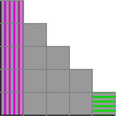
One can generate configurations of
 $X_\Delta $
by distributing black triangles (as in Figure 2) on a white background, so that they do not touch each other (but more complicated configurations are possible).
The triangle
 $T_4$
, illustrating that X is not strongly irreducible: the left column and the right cell are not independent (colour online).

We are going to show that
 $X_\Delta $
is ramified. The first step is to prove that it is not strongly irreducible.
Proposition 5.5. The subshift
 $X_\Delta $
is not strongly irreducible.
Proof. For each
 $r\geq 1$
, the cell
 $(0,0)$
and the column
 $\{(-r,k):0\leq k\leq r\}$
are not independent and their distance is r. Indeed, colouring the column in black forces the whole triangle
 $T_r=\{(x,y):-r\leq x\leq 0,0\leq y\leq r-x\}$
, and in particular the cell
 $(0,0)$
, to be black as well (see Figure 2).
The black triangles can then be used as building blocks to define ramifications.
Proposition 5.6. The subshift
 $X_\Delta $
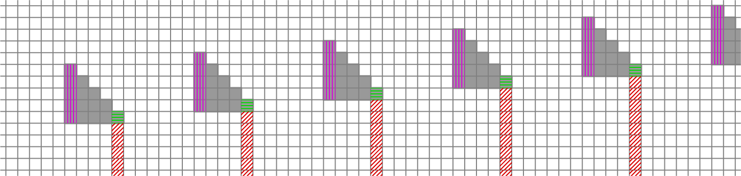
is ramified.
Proof. We build ramifications illustrated in Figure 3. Let
 $r\in \mathbb {N}$
and
 $V_r=\{(n,1):n\geq r+2\}$
, which is an infinite set of pairwise independent vectors. Let
 $F=\{(0,0)\}$
and
 $u=(0,-1)$
. For each r and each
 $v\in V_r$
, we build an
 $(r,v)$
-ramification x by putting a black triangle
 $T_r$
at each multiple of v, everything else being white. Precisely, for each
 $\unicode{x3bb} \in \mathbb {Z}$
, the cells in
 $\unicode{x3bb} v+T_r$
are black, the other cells are white.
A ramification: the cells
 $\unicode{x3bb} v$
are in green, the cells
 $\unicode{x3bb} v+\mu u$
,
 $\mu>0$
, are in red. In a black triangle, the purple and green regions are correlated, and the content of a red cell cannot be grafted in a green cell without changing the purple region (green cells have horizontal hatches, purple cells have vertical hatches and red cells have diagonal hatches) (colour online).

First, x is a valid configuration because the copies of
 $T_r$
are separated by white cells, so they do not create forbidden patterns: if
 $\unicode{x3bb} \neq \unicode{x3bb} '$
and
 $s,t\in T_r$
, then
 $d(\unicode{x3bb} v+s,\unicode{x3bb} ' v+t)=|(\unicode{x3bb} -\unicode{x3bb} ')v+(s-t)|\geq |v|-\mathop {\mathrm {diam}}(T_r)\geq (r+2)-r=2$
, so two cells from different triangles cannot belong to the forbidden pattern, which has diameter
 $1$
.
For
 $\mu>0$
,
 $\mu u=(0,-\mu )\notin T_r$
so the cells
 $\unicode{x3bb} v+\mu u$
are white. The white cell, seen as an F-pattern, appears at position
 $\unicode{x3bb} v+\mu u$
but cannot be r-grafted in x at any position
 $\unicode{x3bb} v$
. We have shown that x is an
 $(r,v)$
-ramification and that X is ramified.
The argument to prove that a subshift X is ramified will always follow the same structure as in this example.
-
• First, show that X is not strongly irreducible by identifying for each
$r\in \mathbb {N}$
two regions F and G at distance larger than r from each other that are not independent. We do so by finding valid F-patterns
$\pi _F,\pi ^{\prime }_F$
and a valid G-pattern
$\pi _G$
such that
$\pi _F\cup \pi _G$
is valid but
$\pi ^{\prime }_F\cup \pi _G$
is not valid (in the pictures, G will be coloured in purple with vertical hatches and F will be coloured in green with horizontal hatches). -
• For a suitable choice of u and v, build an
$(r,v)$
-ramification of period v obtained by placing the pattern
$\pi _F\cup \pi _G$
at each position
$\unicode{x3bb} v$
, the pattern
$\pi ^{\prime }_F$
at each position
$\unicode{x3bb} v+\mu u$
with
$\mu>0$
and filling all the other cells to obtain a valid configuration (the translated version of F at positions
$\unicode{x3bb} v+\mu u$
,
$\mu>0$
, will be coloured in red with diagonal hatches).


In the pictures, a red region cannot be grafted in a green region without changing the purple region.
5.2.2 A non-example: the checkerboard
To better understand the notion of ramification and ramified subshift, it is useful to examine a simple subshift which is not ramified.
Consider the checkerboard subshift
 $X\subseteq \{0,1\}^{\mathbb {Z}^2}$
containing only two configurations
 $x,y$
defined by
 $x_{(i,j)}=i+j\mod 2$
and
 $y_{(i,j)}=i+j+1\mod 2$
.
First, X is not strongly irreducible because for each r, the cells
 $(0,0)$
and
 $(2r+1,0)$
are correlated: each cell can be filled with a
 $0$
, but not in a common configuration.
However, X is not ramified. Assume otherwise and let x be an
 $(r,v)$
-ramification for some
 $r,v$
, witnessed by
 $F,u$
. Choose some arbitrary
 $\unicode{x3bb} $
and
 $\mu>0$
, where
 $\mu $
is even (for instance,
 $\unicode{x3bb} =0,\mu =2$
). The F-pattern appearing in x at position
 $\unicode{x3bb} v+\mu u$
coincides with the F-pattern appearing in x at position
 $\unicode{x3bb} v$
, so it can be r-grafted (and even
 $0$
-grafted) at that position, contradicting the definition of a ramification.
5.3 An obstruction to being in
$\mathscr {L}^0$

We state the main result of this section, which gives a way of showing that a subshift is not in
 $\mathscr {L}^0$
when that subshift is weakly mixing.
Theorem 5.7. (An obstruction to being in
$\mathscr {L}^0$
)

Let X be a
 $\mathbb {Z}^2$
-subshift. If X is ramified and weakly mixing, then
 $X\notin \mathscr {L}^0$
.
The rest of this section is devoted to the proof of this result.
5.3.1 Uniform case
We first show that a ramified subshift cannot be a factor of a product of fullshifts and periodic shifts. To do so, we prove that finite products of fullshifts and periodic shifts are not ramified, and that factor maps send non-ramified subshifts to non-ramified subshifts.
The ‘uniformity’ in the title of this section refers to the fact that factor maps are uniform local functions, with the same rule in each cell. In the next section, we will consider the case of arbitrary, non-uniform local functions. Strictly speaking, the results from this section are implied by the results in the next section, but we prefer to present both because the first ones are easier to understand.
Theorem 5.8. Let X be a
 $\mathbb {Z}^2$
-subshift. If X is ramified, then X not a factor of
 $A^{\mathbb {Z}^2}\times \prod _{i=1}^kA^{\mathbb {Z}^2/u_i\mathbb {Z}}$
, with each
 $u_i\neq 0$
.
We are going to need the following lemma. In the plane, given lines
 $L_0,\ldots ,L_k$
going through the origin and a direction v which is not colinear to any
 $L_i$
, it is obvious that there exists a line with direction vector v intersecting each
 $L_i$
, which does not contain the origin. The next lemma states that it also holds when all the coefficients are integers.
Lemma 5.9. Let
 $u_0,u_1,\ldots ,u_k\in \mathbb {Z}^2$
, with
 $k\geq 1$
. Let
 $v\in \mathbb {Z}^2$
be independent of each
 $u_i$
individually. There exist
 $\unicode{x3bb} _1, \unicode{x3bb} _2,\ldots ,\unicode{x3bb} _k$
and
 $\mu>0$
such that each
 $\mu u_0-\unicode{x3bb} _iv$
is a multiple of
 $u_i$
.
Proof. We show that there exist non-zero integers
 $n_0,\ldots ,n_k$
such that the pairwise differences of
 $n_iu_i$
are multiples of v. If
 $n_0<0$
, then we replace each
 $n_i$
by
 $-n_i$
. We then take
 $\mu =n_0$
and
 $\unicode{x3bb} _i$
such that
 $n_0u_0-n_iu_i=\unicode{x3bb} _i v$
.
First, consider the case when
 $k=1$
. As
 $\mathbb {Z}^2$
has rank
 $2$
as a
 $\mathbb {Z}$
-module, there is a non-trivial combination
 $n_0u_0-n_1u_1+nv=0$
. As v is independent of each
 $u_i$
individually, one has
 $n_0\neq 0$
and
 $n_1\neq 0$
, and the difference of
 $n_0u_0$
and
 $n_1u_1$
is a multiple of v.
Let us now consider the general case
 $k\geq 2$
. For each i from
 $1$
to k, the previous argument applied to
 $u_0$
and
 $u_i$
provides non-zero coefficients
 $n^i_0$
and
 $n^i_1$
such that
 $n^i_0u_0-n^i_1u_i$
is a multiple of v. Let
 $n_0=\prod _j n^j_0$
and
 $n_i=n^i_1\prod _{j\neq i}n^j_0$
. All these coefficients are non-zero and
 $n_0u_0-n_iu_i=(n^i_0u_0-n^i_1u_i)\prod _{j\neq i}n^j_0$
is a multiple of v.
Proposition 5.10. Let
 $X=A^{\mathbb {Z}^2}\times \prod _{i=1}^kA^{\mathbb {Z}^2/u_i\mathbb {Z}}$
with
 $u_i\neq 0$
. X is not ramified.
Proof. A configuration
 $x\in X$
is
 $(x_0,\ldots ,x_k)$
with each
 $x_i\in X_i$
. Let A be the finite alphabet such that
 $X\subseteq A^{\mathbb {Z}^2}$
.
Let v be independent of each
 $u_i$
and x be a
 $(0,v)$
-ramification, with
 $u,F$
. We apply Lemma 5.9, giving
 $\unicode{x3bb} _1,\ldots ,\unicode{x3bb} _k$
and
 $\mu>0$
such that
 $\mu u-\unicode{x3bb} _iv$
is a multiple of
 $u_i$
. Let
 $\unicode{x3bb} _0~=~0$
,
 $L^+=\max _{0\leq i\leq k}\unicode{x3bb} _i$
,
 $L^-=\min _{0\leq i\leq k}\unicode{x3bb} _i$
and
 $L=L^+-L^-+1$
.
We define a colouring of
 $[0,N]$
, where
 $N=N(A^F,L)$
is given by Van der Waerden’s theorem (Theorem A.1). Assign to n the F-pattern
 $\pi _n\in A^F$
appearing at position
 $nv$
in x. By Van der Waerden’s theorem, this colouring admits a monochromatic arithmetic progression of length L, that is, there exist a and
 $b>0$
such that all
 $(a+\unicode{x3bb} b)$
have the same colour,
 $\unicode{x3bb} \in [L^-,L^+]$
. Let
 $\pi $
be the common F-pattern appearing at these positions
 $(a+\unicode{x3bb} b)v$
. In particular, if
 $p_i=(a+\unicode{x3bb} _i b)v$
and
 $q\in F$
, then
 $$ \begin{align} x(p_i+q)=\pi(q) \end{align} $$
does not depend on i.
Let
 $p=av+b\mu u$
and
 $\xi $
be the F-pattern appearing at position p in x. We claim that
 $\xi $
can be
 $0$
-grafted into x at position
 $p_0$
. In other words, if we define
 $x'\in A^E$
by
 $$ \begin{align*} x'(p_0+q)=\begin{cases} \xi(q)=x(p+q)&\text{if }q\in F,\\ x(p_0+q)&\text{otherwise,} \end{cases} \end{align*} $$
then we show that
 $x'$
belongs to X. Note that
 $x^{\prime }_0\in X_0$
because
 $X_0$
is the fullshift. We claim that for
 $i\geq 1$
, one has
 $x^{\prime }_i=x_i\in X_i$
, from which it will follow that
 $x'\in X$
.
We use the fact that
 $p-p_i=b(\mu u-\unicode{x3bb} _iv)$
, which is a multiple of
 $u_i$
, and that
 $x_i\in X_i$
is
 $u_i$
-periodic, so
 $x_i(p+q)=x_i(p_i+q)$
for all q.
If
 $q\notin F$
, then
 $x'(p_0+q)=x(p_0+q)$
by definition of
 $x'$
. If
 $q\in F$
and
 $i\geq 1$
, then
 $$ \begin{align*} x^{\prime}_i(p_0+q)&=x_i(p+q)\quad\,\text{by definition of }x',\\ &=x_i(p_i+q)\quad\text{as }p-p_i\text{ is a multiple of }u_i,\\ &=x_i(p_0+q)\quad\text{as }x(p_i+q)=\pi(q)=x(p_0+q)\text{ by (5.1).} \end{align*} $$
As a result,
 $x^{\prime }_i=x_i\in X_i$
for
 $i\geq 1$
, so
 $x\in X$
.
We have shown that the F-pattern appearing at position
 $p=av+b\mu u$
in x can be
 $0$
-grafted into x at position
 $p_0=av$
, contradicting the assumption that x is a
 $(0,v)$
-ramification.
Being ramified is indeed a conjugacy invariant, as shown by the next result.
Proposition 5.11. If Y is a factor of X and Y is ramified, then X is ramified as well.
Proof. Let
 $f:X\to Y$
be a factor map and
 $k\in \mathbb {N}$
be such that each
 $p\in \mathbb {Z}^2$
is determined by its neighbourhood
 $\mathcal {N}(p,k)$
. For
 $r\in \mathbb {N}$
, let v be such that Y admits an
 $(r+2k,v)$
-ramification
 $y\in Y$
, witnessed by u and F. Let
 $x\in X$
be such that
 $f(x)=y$
. We claim that x is an
 $(r,v)$
-ramification, witnessed by u and
 $W:=\mathcal {N}(F,k)$
.
Let
 $\unicode{x3bb} $
and
 $\mu>0$
be integers. Assume for a contradiction that the W-pattern appearing at position
 $\unicode{x3bb} v+\mu u$
in x can be grafted into x at position
 $\unicode{x3bb} v$
, let
 $x'\in X$
be the result of this graft and
 $y'=f(x')$
. As
 $x'$
coincides with x outside
 $\mathcal {N}(\unicode{x3bb} v+W,r)=\mathcal {N}(\unicode{x3bb} v+F,r+k)$
,
 $y'$
coincides with y outside
 $\mathcal {N}(\unicode{x3bb} v+F,r+2k)$
. The F-pattern appearing at position
 $\unicode{x3bb} v$
in
 $y'$
is the F-pattern appearing at position
 $\unicode{x3bb} v+\mu u$
in y, so
 $y'$
witnesses that this pattern can be
 $(r+2k)$
-grafted into y, which contradicts the assumption.
Given
 $r\in \mathbb {N}$
, there exist infinitely many vectors v such that Y admits an
 $(r+2k,v)$
-ramification and X admits an
 $(r,v)$
-ramification for each such v.
These results imply Theorem 5.7.
5.3.2 Non-uniform case
Our next goal is to extend Theorem 5.8 to show that a ramified subshift cannot be the image of a product of fullshifts and periodic shifts by a local function. Local functions do not necessarily play well with ramifications, so we need to refine the invariant property of being ramified. The idea is that local functions are actually uniform on arbitrarily large regular grids, by the Gallai–Witt theorem (Theorem A.2). Using this observation, we show that they preserve a finite version of ramifications. We start defining this finite version, which is unfortunately rather technical and non-intuitive, but makes the argument go through.
Definition 5.12. Let
 $r\in \mathbb {N}$
and
 $v\in \mathbb {Z}^2$
. A subshift X is finitely
 $(r,v)$
-ramified if there exist
 $u\in \mathbb {Z}^2$
and
 $F\subseteq \mathbb {Z}^2$
such that for all
 $K\in \mathbb {N}$
, there exist
 $x\in X$
and
 $\alpha>0$
such that for all
 $\unicode{x3bb} \in [-K,K]$
and
 $\mu \in [1,K]$
, the F-pattern appearing at position
 $\unicode{x3bb} \alpha v+\mu \alpha u$
in x cannot be r-grafted into x at position
 $\unicode{x3bb} \alpha v$
.
A subshift X is finitely ramified if for all
 $r\in \mathbb {N}$
and for infinitely many pairwise independent vectors v, X is finitely
 $(r,v)$
-ramified.
Remark 5.13. (Ramified implies finitely ramified)
If X admits an
 $(r,v)$
-ramification, then X is finitely
 $(r,v)$
-ramified. Let
 $x_0$
be such an
 $(r,v)$
-ramification. Given
 $K\in \mathbb {N}$
, one easily checks that
 $x=x_0$
and
 $\alpha =1$
satisfy the definition above.
Therefore, if X is ramified, then X is finitely ramified.
Theorem 5.14. Let X be a
 $\mathbb {Z}^2$
-subshift. If X is ramified, then X is not the image of any
 $A^{\mathbb {Z}^2}\times \prod _{i=1}^kA^{\mathbb {Z}^2/u_i\mathbb {Z}}$
by a local function.
This result will directly follow from the next results, which refine Propositions 5.10 and 5.11.
Proposition 5.15. Let X be a finite product of fullshifts and periodic shifts. X is not finitely ramified.
Proof. If X is a fullshift, then it is strongly irreducible so it is not finitely ramified. We now assume that
 $X=\prod _{i=0}^kX_i$
, where
 $k\geq 1$
,
 $X_0$
is a fullshift and for
 $1\leq i\leq k$
,
 $X_i$
is a periodic shift of period
 $u_i\neq 0$
. A configuration
 $x\in X$
is
 $(x_0,\ldots ,x_k)$
with each
 $x_i\in X_i$
. Let A be the finite alphabet such that
 $X\subseteq A^{\mathbb {Z}^2}$
.
Let v be independent of each
 $u_i$
and such that X is finitely
 $(0,v)$
-ramified, using
 $u,F$
. Let
 $u_0=u$
. We apply Lemma 5.9, giving
 $\unicode{x3bb} _1,\ldots ,\unicode{x3bb} _k$
and
 $\mu>0$
such that each
 $\mu u-\unicode{x3bb} _iv$
is a multiple of
 $u_i$
. Let
 $\unicode{x3bb} _0=0$
,
 $L^+=\max _i\unicode{x3bb} _i$
,
 $L^-=\min _i\unicode{x3bb} _i$
and
 $L=L^+-L^-+1$
.
Let
 $N=N(A^F,L)$
be given by the Van der Waerden theorem (Theorem A.1) and
 $K=N\mu $
. There is
 $x\in X$
and
 $\alpha>0$
witnessing the finite
 $(0,v)$
-ramifications.
We define a colouring of
 $[0,N]$
. Assign to each
 $n\in [0,N]$
the F-pattern
 $\pi _n\in A^F$
appearing at position
 $n\alpha v$
in x. By the Van der Waerden theorem, this colouring admits a monochromatic arithmetic progression of length L, that is, there exist a and
 $b\geq 1$
such that all
 $(a+\unicode{x3bb} b)$
have the same colour,
 $\unicode{x3bb} \in [L^-,L^+]$
(in the trivial case when
 $L=1$
, we can take
 $b=1$
). Let
 $\pi $
be the common F-pattern appearing at these positions
 $(a+\unicode{x3bb} b)\alpha v$
. In particular, if
 $p_i=(a+\unicode{x3bb} _i b)\alpha v$
and
 $q\in F$
, then
 $\pi (q)=x(p_i+q)$
does not depend on i.
Observe that
 $a\in [-K,K]$
and
 $b\mu \in [1,K]$
: indeed,
 $a=a+\unicode{x3bb} _0 b\in [0,N]$
and
 $b\leq N/(L-1)\leq N$
(if
 $L=1$
, then
 $b=1=N$
).
Let
 $p=a\alpha v+b\mu \alpha u$
and
 $\xi $
be the F-pattern appearing at position p in x. We claim that
 $\xi $
can be
 $0$
-grafted into x at position
 $p_0$
. In other words, if we define
 $x'\in A^E$
by
 $$ \begin{align*} x'(p_0+q)=\begin{cases} x(p+q)&\text{if }q\in F,\\ x(p_0+q)&\text{otherwise,} \end{cases} \end{align*} $$
then
 $x'$
belongs to X. Note that
 $x^{\prime }_0\in X_0$
because
 $X_0$
is the fullshift. We claim that for
 $i\geq 1$
, one has
 $x^{\prime }_i=x_i\in X_i$
, from which it follows that
 $x'\in X$
.
We use the fact that
 $p-p_i=b(\mu \alpha u-\unicode{x3bb} _i \alpha v)$
, which is a multiple of
 $u_i$
, so
 $x_i(p+q)=x_i(p_i+q)$
for all q.
If
 $q\notin F$
, then
 $x'(p_0+q)=x(p_0+q)$
by definition of
 $x'$
. If
 $q\in F$
and
 $i\geq 1$
, then
 $$ \begin{align*} x^{\prime}_i(p_0+q)&=x_i(p+q)\quad\,\text{by definition of }x',\\ &=x_i(p_i+q)\quad\text{as }p-p_i\text{ is a multiple of }u_i,\\ &=x_i(p_0+q)\quad\text{as }x(p_i+q)=\pi(q)=x(p_0+q). \end{align*} $$
As a result,
 $x^{\prime }_i=x_i\in X_i$
for
 $i\geq 1$
, so
 $x\in X$
.
We have shown that the F-pattern appearing at position
 $p=a\alpha v+b\mu \alpha u$
in x can be
 $0$
-grafted into x at position
 $p_0=a\alpha v$
.
One has
 $|a|\leq K$
and
 $|b\mu |\leq K$
so it contradicts the property of finite
 $(0,v)$
- ramifications.
Proposition 5.16. Let
 $X,Y$
be subshifts, such that Y is the image of X by a local function. If Y is ramified, then X is finitely ramified.
Proof. Let
 $f:X\to Y$
of radius k. Let
 $r\in \mathbb {N}$
and v be such that Y has an
 $(r+2k,v)$
-ramification y, witnessed by u and F. We define
 $W=\mathcal {N}(F,k)$
, which is the region that determines F, and show that X is finitely
 $(r,v)$
-ramified, witnessed by u and W.
Let
 $K\in \mathbb {N}$
and
 $G_K=\{\unicode{x3bb} v+\mu u:\unicode{x3bb} \in [-K,K],\mu \in [1,K]\}$
.
To each
 $p\in \mathbb {Z}^2$
, we associate the rule that determines the F-pattern appearing at position p in
 $f(x)$
from the W-pattern appearing at position p in x. If A and B are the finite alphabets underlying X and Y, respectively, then a rule is an element of the finite set
 $(B^F)^{A^W}$
. By the Gallai-Witt theorem (Theorem A.2), there exist
 $a\in \mathbb {Z}^2$
and
 $\alpha>0$
such that all the cells in
 $a+\alpha G_K$
have the same rule. The shift-invariance of X and Y enables us to get rid of a as follows: the function
 $g=\sigma ^a\circ f\circ \sigma ^{-a}$
is a surjective local function of radius k, it surjectively sends X to Y and all the cells in
 $\alpha G_K$
have the same rule.
Let
 $x\in X$
be such that
 $g(x)=y$
, we show that x and
 $\alpha $
satisfy the finite ramification property for X.
Assume for a contradiction that for some
 $\unicode{x3bb} \in [-K,K]$
and
 $\mu \in [1,K]$
, the W-pattern appearing at position
 $p=\unicode{x3bb} \alpha v+\mu \alpha u$
can be r-grafted into x at position
 $p_0=\unicode{x3bb} \alpha v$
, let
 $x'$
be the result of this r-graft and define
 $y'=g(x')$
. Note that
 $p,p_0\in \alpha G_K$
so the function g has the same rules at positions p and
 $p_0$
. This property and the fact that the W-pattern at position p in x coincides with the W-pattern at position
 $p_0$
in
 $x'$
imply that the F-pattern
 $\pi $
appearing at position p in y coincides with the F-pattern at position
 $p_0$
in
 $y'$
. As
 $x'$
coincides with x outside
 $\mathcal {N}(p_0+W,r)=\mathcal {N}(p_0+F,r+k)$
and g has radius k,
 $y'=g(x')$
coincides with
 $y=g(x)$
outside
 $\mathcal {N}(p_0+F,r+2k)$
. As
 $y'\in Y$
, it shows that the
 $\pi $
can be
 $(r+2k)$
-grafted into y at position
 $p_0$
, which contradicts the assumption that y is an
 $(r+2k,v)$
-ramification for Y.
Finally, given r, there are infinitely many pairwise independent vectors v such that Y has
 $(r+2k,v)$
-ramifications and we have shown that X is finitely
 $(r,v)$
-ramified for each such
 $(r,v)$
. As a result, X is finitely ramified.
We have all the ingredients to prove Theorem 5.7.

5.4 Applications
We are going to apply Theorem 5.7 to a two subshifts.
5.4.1 The triangles
We start with the subshift
 $X_\Delta $
, already analysed in §5.2.1.
Theorem 5.17. The subshift
 $X_\Delta $
is ramified and mixing; therefore, it is not in
 $\mathscr {L}^0$
.
Proof. We have already seen that it is ramified (Proposition 5.6), so let us prove that it is mixing. Let
 $T_n=\{(x,y)\in \mathbb {Z}^2:x,y\geq 0,x+y\leq n\}$
. Any valid
 $T_n$
-pattern can be extended to a valid configuration by making all the other cells white: one easily checks that it does not create a forbidden pattern. If
 $\pi ,\pi '$
are valid
 $T_n$
-patterns, then for all
 $p\in \mathbb {Z}^2$
such that
 $|p|\geq \mathop {\mathrm {diam}}(T_n)+2=n+2$
,
 $\pi \cup \sigma ^p(\pi ')$
is valid because
 $d(T_n,T_n-p)\geq 2$
so the extension of
 $\pi \cup \sigma ^p(\pi ')$
with white cells is a valid configuration: the forbidden pattern has diameter
 $1$
, so it cannot intersect both
 $T_n$
and
 $T_n-p$
.
5.4.2 Domino tilings
We consider the domino tileset shown in Figure 4. It induces a very classical tiling which is a particular case of the dimer model in statistical mechanics. The problem of generating random configurations has been studied in [Reference Janvresse, de la Rue and VelenikJdlRV06, Reference Jockusch, Propp and ShorJPS98, Reference ProppPro03] among others.
The domino tileset.

Theorem 5.18. The domino subshift is ramified and mixing, so it does not belong to
 $\mathscr {L}^0$
.
Proof. Let X be the domino subshift. First, X is not strongly irreducible, as illustrated in Figure 5. For
 $k\in \mathbb {N}$
, the horizontal line
 $H_k=[-k,k]\times \{0\}$
filled with an alternation of
 and
 determines the content of the upper triangle
 $\{(i,j):j\geq 1, |i|+j\leq k+1\}$
, in particular, its tip
 $T_k=(0,k+1)$
. Therefore,
 $T_k$
and
 $H_k$
are correlated and
 $d(T_k,H_k)=k+1$
is arbitrarily large.
The domino subshift is not strongly irreducible: the purple pattern (vertical hatches) determines the content of the green cell (horizontal hatches) (colour online).

Figure 6 shows a ramification. One can build an
 $(r,v)$
-ramification for any r and
 $v=(r,r+2)$
by placing diamonds
 $\{(i,j):|i|+|j+0.5|\leq r+0.5\}$
of width
 $2r+1$
made of vertical tiles and with their tips at the multiples of v, and filling each remaining horizontal half-line with the horizontal tiles
 and
 . The distance between the tip and the lower middle row of the diamond is
 $r+1$
. We take
 $u=(-1,1)$
and
 $F=\{(0,0)\}$
. All the cells
 $\unicode{x3bb} v+\mu u$
, with
 $\mu>0$
, are filled with horizontal tiles, which cannot be r-grafted at
 $\unicode{x3bb} v$
.
An
 $(r,v)$
-ramification with
 $r=4$
and
 $v=(4,6)$
,
 $u=(-1,1)$
and
 $F=\{(0,0)\}$
(colour online).

We finally prove that X is mixing. Let
 $D_k$
be the diamond
 $\{(i,j)\in \mathbb {Z}^2:|i|+|j|\leq k\}$
. We show that if
 $|p|\geq 2k+3$
, then
 $D_k$
and
 $p+D_k$
are independent.
Let
 $\pi $
be a valid
 $D_k$
-pattern. We first extend
 $\pi $
to a
 $D_{k+1}$
-pattern as follows. Let
 $(i,j)\in D_{k+1}\setminus D_k$
. If
 $i\geq 1$
, then we do not use ; if
 $i\leq -1$
, then we do not use ; if
 $i=0$
, then we do not use both tiles. Here,
 $\pi '$
has the property that any vertical edge on its boundary is white. We can therefore extend
 $\pi '$
to a valid pattern
 $\xi $
on
 $[-k-1,k+1]\times \mathbb {Z}$
by using and only, in a deterministic way. The boundaries of
 $\xi $
are white.
Let now
 $p=(i,j)$
be such that
 $|p|\geq 2k+3$
, and let
 $\pi ,\pi '$
be valid patterns on
 $D_k$
and
 $p+D_k$
, respectively. There are two cases:
 $|i|\geq 2k+3$
or
 $|j|\geq 2k+3$
.
First, assume that
 $|i|\geq 2k+3$
. One can extend
 $\pi ,\pi '$
to valid patterns
 $\xi ,\xi '$
on
 $[-k-1, k+1]\times \mathbb {Z}$
and
 $[i-k-1,i+k+1]\times \mathbb {Z}$
, respectively, with white boundaries. They do not intersect as
 $|i|\geq 2k+3$
. The rest of the plane can be filled with and .
Now, assume that
 $|j|\geq 2k+3$
. It reduces to the first case by applying a rotation by 90 degrees.
6 Transitions
We now develop a technique to prove that a subshift does not belong to
 $\mathscr {L}^1$
. There are many subshifts in which typical configurations exhibit a transition between two regions that use different sets of tiles. We show that this type of subshift does not belong to
 $\mathscr {L}^1$
.
6.1 An obstruction to being in
$\mathscr {L}^1$

The simplest example of a subshift witnessing a transition is the one-dimensional SFT on the alphabet
 $\{$
,
 $\}$
with forbidden pattern
 .
We denote by
 $X_{\overline {\mathbb {Z}}}$
the induced
 $\mathbb {Z}$
-subshift, because it is conjugate to
 $\overline {\mathbb {Z}}=\mathbb {Z}\cup \{-\infty ,+\infty \}$
whose topology is generated by the basis of open sets
 $\{n\}$
,
 $[n,+\infty ]$
and
 $[-\infty ,n]$
for
 $n\in \mathbb {Z}$
, and with the continuous
 $\mathbb {Z}$
-action
 $$ \begin{align*} p\cdot n&=p+n\text{ for finite }n,\\ p\cdot (+\infty)&=+\infty,\\ p\cdot (-\infty)&=-\infty. \end{align*} $$
The conjugacy map
 $F:\overline {\mathbb {Z}}\to X_{\overline {\mathbb {Z}}}$
sends
 $n\in \overline {\mathbb {Z}}$
to the configuration which is white on the cells
 $p<-n$
and black on the cells
 $p\geq -n$
. In particular, it sends
 $-\infty $
to the white configuration and
 $+\infty $
to the black configuration.
The next result shows in particular that
 $X_{\overline {\mathbb {Z}}}$
is not the image of a narrow function. It relies of the following simple observation: given a continuous function, if two output regions do not communicate, that is, are determined by disjoint input regions, then they are independent. We recall that once a continuous function
 $f:A^{\mathbb {N}}\to B^E$
is fixed, to each output position
 $p\in E$
is associated its input window
 $\mathcal {W}_f(p)\subseteq \mathbb {N}$
. More generally, to each output region
 $F\subseteq E$
, we associate its input window
 $\mathcal {W}_f(F)=\bigcup _{p\in F}\mathcal {W}_f(p)$
. The values of an input
 $x\in A^{\mathbb {N}}$
on
 $\mathcal {W}_f(F)$
determine the value of the output
 $f(x)$
on F.
Lemma 6.1. Let
 $f:A^{\mathbb {N}}\to B^E$
be a narrow function and X be the image of f. Let
 $F, G\subseteq E$
. If
 $\mathcal {W}_f(F)\cap \mathcal {W}_f(G)=\emptyset $
, then F and G are independent with respect to X.
Proof. Let
 $\pi _F,\pi _G$
be a valid patterns on
 $F,G$
, respectively. There exist a
 $\mathcal {W}_f(F)$
-pattern
 $\xi _F$
and a
 $\mathcal {W}_f(G)$
-pattern
 $\xi _G$
such that
 $f([\xi _F])\subseteq [\pi _F]$
and
 $f([\xi _G])\subseteq [\pi _G]$
. As
 $\mathcal {W}_f(F)$
and
 $\mathcal {W}_f(G)$
are disjoint, there exists
 $x\in A^{\mathbb {N}}$
extending
 $\xi _F\cup \xi _G$
, so
 $f(x)$
extends
 $\pi _F\cup \pi _G$
, which is then valid. Therefore, F and G are independent.
Proposition 6.2. Let A be a finite alphabet. If
 $f:A^{\mathbb {N}}\to X_{\overline {\mathbb {Z}}}$
is a narrow function, then its image is finite. Moreover, if f is r-narrow, then
 $$ \begin{align*} |\mathrm{im}(f)|\leq |A|^{{r(r+1)}/{2}}. \end{align*} $$
In particular,
 $X_{\overline {\mathbb {Z}}}$
is not the image of a narrow function.
Proof. We prove the result by induction on r. Let
 $b(r)=|A|^{{r(r+1)}/{2}}$
. For
 $r=0$
, a
 $0$
-narrow function is constant, so
 $\mathrm {im}(f)=1=b(0)$
.
Let
 $r\geq 1$
and assume by induction that the result holds for
 $r-1$
. Let
 $f:A^{\mathbb {N}}\to X_{\overline {\mathbb {Z}}}$
and let
 $E=\{p\in \mathbb {Z}:\text { there exists } x,y\in \mathrm {im}(f),x(p)\neq y(p)\}$
be the set of cells to which f assigns several values. If
 $E=\emptyset $
, then f is constant so
 $|\mathrm {im}(f)|=1\leq b(r)$
. Assume from now on that
 $E\neq \emptyset $
.
Let us show that for every pair of distinct elements
 $p,q\in E$
, the cells p and q are correlated in
 $\mathrm {im}(f)$
. We can assume without loss of generality that
 $p<q$
. As
 $p,q\in E$
, there exist
 $x,y\in \mathrm {im}(f)$
such that
 $x(p)=$
and
 $y(q)=$
. However, there is no
 $z\in \mathrm {im}(f)$
such that
 $z(p)=x(p)$
and
 $z(q)=y(q)$
. We have shown that p and q are correlated in
 $\mathrm {im}(f)$
. Therefore, the input windows
 $\mathcal {W}_f(p)$
and
 $\mathcal {W}_f(q)$
of p and q with respect to f must have non-empty intersection. Note that for
 $p\notin E$
,
 $\mathcal {W}_f(p)=\emptyset $
because
 $x(p)$
is constant for
 $x\in \mathrm {im}(f)$
.
Fix some
 $p\in E$
and let
 $\pi $
be an input
 $\mathcal {W}_f(p)$
-pattern. We define
 $f_\pi :A^{\mathbb {N}}\to \overline {\mathbb {Z}}$
by
 $f_\pi (x)=f(x')$
, where
 $x'$
is obtained from x by replacing the content of
 $\mathcal {W}_f(p)$
by
 $\pi $
. The function
 $f_\pi $
is
 $(r-1)$
-narrow. Indeed, every output cell q is determined by
 $\mathcal {W}_f(q)\setminus \mathcal {W}_f(p)$
, whose size is at most
 $r-1$
as it is either empty or strictly contained in
 $\mathcal {W}_f(q)$
which has size at most r.
Therefore, by induction hypothesis,
 $\mathrm {im}(f_\pi )\leq b(r-1)$
. One has
 $\mathrm {im}(f)=\bigcup _\pi \mathrm {im}(f_\pi )$
and there are
 $|A|^{|\mathcal {W}_f(p)|}\leq |A|^r$
many
 $\mathcal {W}_f(p)$
-patterns
 $\pi $
, so
 $|\mathrm {im}(f)|\leq |A|^rb(r-1)=b(r)$
.
We now state the main technique that will be used to show that a subshift is not in
 $\mathscr {L}^1$
and which is a direct consequence of the previous results.
Theorem 6.3. (An obstruction to being in
$\mathscr {L}^1$
)

Let X be a
 $\mathbb {Z}^d$
-subshift. If X is weakly mixing and
 $\overline {\mathbb {Z}}$
is a weak factor of X, then
 $X\notin \mathscr {L}^1$
.
Proof. As X is weakly mixing, we can apply Proposition 4.11, so we only need to show that X is not the image of a narrow function. By assumption, there exists weak factor map
 $F:X\to \overline {\mathbb {Z}}$
, which is in particular a narrow function. If X was the image of a narrow function
 $G:A^{\mathbb {N}}\to X$
, then
 $\overline {\mathbb {Z}}$
would be the image of the narrow function
 $F\circ G$
, contradicting Proposition 6.2.
6.2 Application
The simplest subshift to which Theorem 6.3 can be applied is the two-dimensional version of the SFT discussed in the previous section (note that the one-dimensional version is countable, so it belongs to
 $\mathscr {L}^0\subseteq \mathscr {L}^1$
).
Proposition 6.4. Let X be the
 $\mathbb {Z}^2$
-SFT on the alphabet
 $\{$
,
 $\}$
with forbidden pattern . X weak factors to
 $\overline {\mathbb {Z}}$
and is weakly mixing; therefore,
 $X\notin \mathscr {L}^1$
.
Proof. The function that extracts the first row of a configuration of X is a weak factor map to the
 $\mathbb {Z}$
-subshift
 $X_{\overline {\mathbb {Z}}}$
, via the homomorphism
 $\varphi :\mathbb {Z}\to \mathbb {Z}^2$
defined by
 $\varphi (p)=(p,0)$
.
It is weakly mixing, because two regions that do not intersect a common row are independent. In particular, for each n,
 $S_n$
and
 $(0,n)+S_n$
are independent.
We then apply Theorem 6.3, implying
 $X\notin \mathscr {L}^1$
.
6.3 Other subshifts
In §5, we identified two subshifts that do not belong to
 $\mathscr {L}^0$
. We expect them to belong to
 $\mathscr {L}^1$
either, but have not been able to prove it so far. The technique used in this section, namely Theorem 6.3, cannot be applied to them because they are all mixing and Proposition 3.10 prevents
 $\overline {\mathbb {Z}}$
from being a weak factor of a mixing subshift. Indeed,
 $\overline {\mathbb {Z}}$
is neither periodic nor mixing.
We present two other arguments showing that a subshift does not belong to
 $\mathscr {L}^1$
.
6.3.1 Stacks
Consider the SFT
 $X\subseteq \{0,1,2\}^{\mathbb {Z}^2}$
with forbidden patterns
 $\begin {smallmatrix}1\\0\end {smallmatrix},\begin {smallmatrix}2&0\end {smallmatrix}, \begin {smallmatrix}0&2\end {smallmatrix},\begin {smallmatrix}2&1\end {smallmatrix}$
and
 $\begin {smallmatrix}1&2\end {smallmatrix}$
. A valid configuration is obtained by filling certain rows with
 $2$
s and by filling each portion of each column lying between two occurrences of
 $2$
, by a stack of
 $1$
s with a stack of
 $0$
s above it.
Let us first show that
 $\overline {\mathbb {Z}}$
is not a weak factor of X, implying that Theorem 6.3 cannot be applied.
Proposition 6.5. Let
 $X,Y$
be subshifts and assume that Y is a weak factor of X. If the strongly periodic configurations of X are dense in X, then the strongly periodic configurations of Y are dense in Y.
Proof. Let X be a
 $\mathbb {Z}^d$
-subshift, Y a
 $\mathbb {Z}^e$
-subshift,
 $f:X\to Y$
a weak factor map coming with
 $\varphi :\mathbb {Z}^e\to \mathbb {Z}^d$
. If
 $x\in X$
is strongly periodic, that is, its orbit
 $O_x:=\{\sigma ^p(x):p\in \mathbb {Z}^d\}$
is finite, then the orbit of
 $f(x)$
is finite because it is contained in
 $f(O_x)$
: indeed,
 $\sigma ^p(f(x))=f(\sigma ^{\varphi (p)}(x))\in f(O_x)$
. As f is continuous, it sends a dense set to a dense set.
Our subshift X contains a dense set of strongly periodic configurations: given a valid
 $S_n$
-pattern
 $\pi $
, extend
 $\pi $
on
 $[0,n-1]\times [0,n]$
by adding a row filled with
 $2$
s at the top and copy this pattern at each point of the grid
 $(n,0)\mathbb {Z}+(0,n+1)\mathbb {Z}$
, yielding a strongly periodic configuration extending
 $\pi $
. However, in
 $\overline {\mathbb {Z}}$
, the only strongly periodic configurations are its two fixed points, which are not dense.
We now show that
 $X\notin \mathscr {L}^1$
, using a different but related argument.
Proposition 6.6. We have
 $X\notin \mathscr {L}^1$
.
Proof. We show that X is not the image of a narrow function and that X is weakly mixing, which implies that
 $X\notin \mathscr {L}^1$
by Proposition 4.11.
Let
 $f:A^{\mathbb {N}}\to X$
be an r-narrow function. Let
 $b_A(r)=|A|^{{r(r+1)}/{2}}$
from Proposition 6.2. Let
 $K\in \mathbb {N}$
be such that
 $p:={b_A(r)}/{K}< 1$
and let
 $N\in \mathbb {N}$
be such that
 $|A|^{r(K+1)}p^N<1$
. Consider the valid pattern
 $\pi =200\cdots 002$
on the vertical line
 $F=\{(0,0),\ldots ,(0,K)\}$
.
We observe that if x is a valid configuration extending
 $\pi $
, then for each
 $i\in \mathbb {Z}$
, the content of the vertical line
 $F_i=\{(i,1),\ldots ,(i,K-1)\}$
can be seen as a configuration of
 $X_{\overline {\mathbb {Z}}}$
, by appending
 $1$
s below and
 $0$
s above and identifying
 $1$
with and
 $0$
with . More formally, this transformation is the function
 $g_i:[\pi ]\cap X\to X_{\overline {\mathbb {Z}}}$
defined by
 $$ \begin{align*} (g_i(x))_p=\begin{cases} 1&\text{if }p\leq 0,\\ x_{(i,p)}&\text{if }0< p<K,\\ 0&\text{if }p\geq K.\\ \end{cases} \end{align*} $$
Observe that
 $g_i$
is
 $1$
-narrow, because one has
 $\mathcal {W}_{g_i}(p)=\{(i,p)\}$
if
 $0<p<K$
and
 $W_{g_i}(p)=\emptyset $
otherwise.
Let
 $\xi $
be a pattern on
 $\mathcal {W}_f(F)$
that is sent to
 $\pi $
under f, and let
 $f_\xi :A^{\mathbb {N}}\to X$
be obtained by first replacing the content of
 $\mathcal {W}_f(F)$
in the input by
 $\xi $
and then applying f, and note that
 $f_\xi $
is r-narrow. For each
 $i\in [1,N]$
, let
 $F_i=\{(i,1),\ldots ,(i,K-1)\}$
and
 $f_i:A^{\mathbb {N}}\to X_{\overline {\mathbb {Z}}}$
be defined by
 $f_i=g_i\circ f_\xi $
. As
 $f_\xi $
is r-narrow and
 $g_i$
is
 $1$
-narrow,
 $f_i$
is r-narrow. By Proposition 6.2, the cardinality of
 $\mathrm {im}(f_i)$
is at most
 $b_A(r)$
. In other words, in
 $\mathrm {im}(f_\xi )$
, there are at most
 $b_A(r)$
ways of filling
 $F_i$
, which is a fraction p of the number of possible contents. Therefore, the fraction of the possible contents of the rectangle
 $R:=F_1\cup \cdots \cup F_N$
reached by
 $f_\xi $
is at most
 $p^N$
. As f is r-narrow,
 $|\mathcal {W}_f(F)|\leq r|F|=r(K+1)$
, so there are at most
 $|A|^{r(K+1)}$
input patterns
 $\xi $
sent to
 $\pi $
, so a fraction of at most
 $|A|^{r(K+1)}p^N<1$
contents of R that are reached by f. Therefore, f is not surjective.
It is easy to see that X is weakly mixing by observing that
 $S_m$
and
 $(0,m+1)+S_m$
are independent. Indeed, if
 $x,y$
are valid configurations, then the configuration z which coincides with x strictly under row m and with y strictly above row m and filled with
 $2$
s on row m is valid. Therefore, any valid pattern on
 $S_m$
and any valid pattern on
 $(0,m+1)+S_m$
together form a valid pattern.
6.3.2 Irrational rotation
We show that the classical Sturmian
 $\mathbb {Z}$
-subshifts encoding irrational rotations on the circle do not belong to
 $\mathscr {L}^1$
. It confirms the intuition that building a valid configuration cannot be achieved in a local way, because all the cells need to share an infinite amount of information, namely the point of the circle that is encoded into the configuration.
We recall the definitions, more details can be found from Pytheas Fogg [Reference Berthe, Ferenczi, Mauduit and SiegelBFMS02, §6.1.2].
Let
 $\mathbb {R}/\mathbb {Z}$
be the circle group. Let
 $\alpha \in (0,1)$
be irrational and let
 $R_\alpha :\mathbb {R}/\mathbb {Z}\to \mathbb {R}/\mathbb {Z}$
be the irrational rotation sending x to
 $x+\alpha \mod 1$
. Consider two partitions of the circle:
 $$ \begin{align*} I_0&=[0,1-\alpha)\quad I^{\prime}_0=(0,1-\alpha],\\ I_1&=[1-\alpha,1)\quad I^{\prime}_1=(1-\alpha,1]. \end{align*} $$
To any
 $x\in \mathbb {R}/\mathbb {Z}$
, we associate the two sequences
 $w(x),w'(x)\in \{0,1\}^{\mathbb {Z}}$
defined by
 $w_n(x)=a$
such that
 $R_\alpha ^n(x)\in I_a$
and
 $w^{\prime }_n(x)=a$
such that
 $R_\alpha ^n(x)\in I^{\prime }_a$
. More directly, these sequences can be defined for
 $x\in [0,1]$
by
 $$ \begin{align*} w_n(x)&=\lfloor (n+1)\alpha+x \rfloor-\lfloor n\alpha+x \rfloor,\\ w^{\prime}_n(x)&=\lceil (n+1)\alpha+x \rceil-\lceil n\alpha+x \rceil. \end{align*} $$
We then consider the subshift containing all these sequences:
 $$ \begin{align*} X_\alpha=\{w(x):x\in [0,1)\}\cup \{w'(x):x\in [0,1)\}. \end{align*} $$
For most x, one has
 $w(x)=w'(x)$
. The two sequence are different only if some
 $n\alpha +x$
is an integer, in which case,
 $w_{n-1}(x)w_n(x)=10$
and
 $w^{\prime }_{n-1}(x)w^{\prime }_n(x)=01$
, and the two sequences coincide elsewhere.
It turns out that
 $X_\alpha $
is not weakly mixing, so we need another argument.
Proposition 6.7. We have
 $X_\alpha \notin \mathscr {L}^1$
.
Proof. Let
 $F\subseteq \mathbb {Z}$
be a finite set and
 $u\in \{0,1\}^F$
a finite pattern. We show that
 $X\cap [u]$
is not the image of a narrow function, which implies that
 $X\notin \mathscr {L}^1$
by Proposition 4.2.
We say that
 $x\in \mathbb {R}/\mathbb {Z}$
is generic if no
 $n\alpha +x$
is an integer. The generic points are dense in the circle, and their images by w and
 $w'$
are dense in
 $X_\alpha $
. Let x be generic such that
 $w(x)=w'(x)$
extends u. For a real number z, let
 $\{z\}=z-\lfloor z \rfloor \in [0,1)$
be its fractional part. Let
 $i_0\in \mathbb {N}$
be such that
 $1-\alpha -2^{-i_0-1}>0$
and
 $\epsilon =\min \{\alpha ,1-\alpha -2^{-i_0-1}\}$
. For each
 $i\geq i_0$
, there exists
 $n_i\in \mathbb {Z}$
such that
 $\{n_i\alpha +x\}\in (1-\alpha -2^{-i},1-\alpha -2^{-i-1})$
. Let v be a finite extension of u which is compatible with
 $w(x)$
and such that if
 $w(y)$
extends v, then
 $|x-y|<\epsilon $
. Let
 $g:X\cap [v]\to \{0,1\}^{\mathbb {Z}}$
send s to
 $i\mapsto s(n_i)$
. We claim that the image of g is an infinite set of non-decreasing binary sequences.
One has
 $w_{n_i}(x)=0$
, so
 $\mathrm {im}(g)$
contains the zero sequence.
Let y be such that
 $w(y)$
extends v. We show that
 $g(w(y))$
is non-decreasing. As
 $|x-y|<\epsilon $
, one has
 $\{n_i\alpha +y\}=\{n_i\alpha +x\}+(y-x)$
because these quantities are equal modulo
 $1$
and both belong to
 $[0,1)$
. If
 $w_{n_i}(y)=1$
, then
 $\{n_i\alpha +y\}\geq 1-\alpha $
, so
 $\{n_{i+1}\alpha +y\}=\{n_{i+1}\alpha +x\}+(y-x)> \{n_i\alpha +x\}+(y-x)=\{n_i\alpha +y\}\geq 1-\alpha $
, so
 $w_{n_{i+1}}(y)=1$
. Therefore,
 $g(w(y))$
is indeed non-decreasing.
We show that
 $g(X\cap [v])$
has infinitely many elements. As x is generic, the function w is continuous at x, so there exists
 $\delta>0$
such that if
 $|x-y|<\delta $
, then
 $w(y)$
extends v. Let
 $i_1$
be such that
 $2^{-i_1}<\delta $
. For
 $i\geq i_1$
, let
 $y=x+1-\alpha -2^{-i}-\{n_i\alpha +x\}$
. One has
 $|x-y|<\delta $
and
 $\{n_i\alpha +y\}=1-\alpha -2^{-i}$
. The sequence
 $g(w(y))$
starts with
 $i 0$
s, followed by
 $1$
s.
The function g is
 $1$
-narrow, because its output at position i is determined by its input at position
 $n_i$
. Therefore, if
 $X\cap [v]$
was the image of a narrow function, then by composing with g, we would obtain a narrow function whose image is an infinite set of non-decreasing sequences, that is, of elements of
 $\overline {\mathbb {Z}}$
, which is a contradiction. As
 $[v]\subseteq [u]$
,
 $X\cap [u]$
is not the image of a narrow function by Proposition 4.2.
7 Subshifts that can be locally generated
We now present examples of subshifts that belong to
 $\mathscr {L}^0$
. We first show that
 $\mathscr {L}^0$
is preserved under higher power presentations. This result will be used in the next arguments.
7.1 Higher power presentations and intertwining
A common way of building a subshift from another one is to gather the cells into rectangular blocks and interpret the content of each block as an element of a larger alphabet. It can be found in [Reference Lind and MarcusLM95, Definition 1.4.4] in the one-dimensional case, where it is called a higher power presentation of the subshift.
This operation sometimes results in a subshift which is easier to analyse. Intuitively, this operation should not affect the possibility of local generation. Indeed, we show that a higher power presentation of a subshift belongs to
 $\mathscr {L}^0$
if and only if the original subshift belongs to
 $\mathscr {L}^0$
. Although intuitive, it turns out that this result is not so straightforward to prove.
Let
 $a=(a_1,\ldots ,a_d)\in \mathbb {Z}^d$
be a vector with positive coordinates and consider the hyper-rectangle
 $R_a=[0,a_1-1]\times \cdots \times [0,a_d-1]$
.
Definition 7.1. To any
 $\mathbb {Z}^d$
-subshift
 $X\subseteq \Sigma ^{\mathbb {Z}^d}$
, we associate its a-higher power presentation
 $[X]_a$
, which is a
 $\mathbb {Z}^d$
-subshift on the alphabet
 $\Gamma :=\Sigma ^{R_a}$
defined as follows. Let
 $F_a:\Sigma ^{\mathbb {Z}^d}\to \Gamma ^{\mathbb {Z}^d}$
be such that
 $F_a(x)_p$
is the
 $R_a$
-pattern appearing at position
 $ap=(a_1p_1,\ldots ,a_dp_d)$
in x. We then define
 $[X]_a=\mathrm {im}(F_a)$
.
The subshift
 $[X]_a$
is always a weak factor X, but not the other way round (see Example 3.8).
The main goal of this section is to show that higher power presentations behave well with respect to the class
 $\mathscr {L}^0$
, as expressed by the next result.
Theorem 7.2. (
$\mathscr {L}^0$
and higher power presentations)

Let
 $a\in \mathbb {Z}^d$
have positive coordinates and X be a
 $\mathbb {Z}^d$
-subshift. One has
 $$ \begin{align*} X\in\mathscr{L}^0\,{\iff}\, [X]_a\in\mathscr{L}^0. \end{align*} $$
The rest of this section is devoted to the proof of Theorem 7.2 and can be skipped at first reading.
Let us start with a result highlighting the role of the compact subshift K in the definition of
 $\mathscr {L}^0$
when it is finite.
Proposition 7.3. (Higher power presentations and factors)
Let
 $X,Y$
be subshifts. The following conditions are equivalent:
-
• Y is a factor of
$K\times X$
for some finite
$\mathbb {Z}^d$
-set K; -
• there exists
$a\in \mathbb {Z}^d$
with positive coordinates such that
$[Y]_a$
is a finite union of factors of
$[X]_a$
.


Proof. Assume that Y is a factor of
 $K\times X$
for some finite
 $\mathbb {Z}^d$
-set K. For each
 $k\in K$
, let
 $f_k:X\to Y$
be defined by
 $f_k(x)=f(k,x)$
. As K is finite, each vector
 $e_i$
of the canonical basis of
 $\mathbb {Z}^d$
has a multiple
 $a_ie_i$
, with
 $a_i>0$
, that acts as the identity on K. Let
 $a=(a_1,\ldots ,a_d)$
. For any
 $p\in \mathbb {Z}^d$
,
 $ap$
acts as the identity on K. It implies that
 $\sigma ^{ap}\circ f_k=f_k\circ \sigma ^{ap}$
:
 $$ \begin{align*} \sigma^{ap}\circ f_k(x)&=\sigma^{ap}\circ f(k,x)\\ &=f(ap\cdot k,\sigma^{ap}(x))\\ &=f(k,\sigma^{ap}(x))\\ &=f_k\circ \sigma^{ap}(x). \end{align*} $$
Let
 $F_X:X\to [X]_a$
and
 $F_Y:Y\to [Y]_a$
be the canonical homeomorphisms, which satisfy
 $\sigma ^p\circ F_Z=F_Z\circ \sigma ^{ap}$
(for
 $Z=X$
or Y). Each function
 $F_Y\circ f_k\circ F_X^{-1}$
is a factor map from
 $[X]_a$
to its image and
 $[Y]_a$
is the finite union over
 $k\in K$
of these images.
Conversely, assume that
 $[Y]_a=\bigcup _{i\in I}f_i([X]_a)$
, where I is finite,
 $f_i:[X]_a\to [Y]_a$
is continuous and commutes with the shift actions. Let
 $K=I\times \mathbb {Z}^d/a\mathbb {Z}^d$
, where I is endowed with the trivial action
 $p\cdot i=i$
. The functions
 $f^{\prime }_i=F_Y^{-1}\circ f_i\circ F_X:X\to Y$
satisfy
 $\sigma ^{ap}\circ f^{\prime }_i\circ \sigma ^{-ap}=f^{\prime }_i$
, which implies that for any
 $p\in \mathbb {Z}^d$
,
 $\sigma ^p\circ f^{\prime }_i\circ \sigma ^{-p}$
only depends on the equivalence class
 $[p]$
of p modulo
 $a\mathbb {Z}^d$
. Therefore, the following function
 $g:K\times X\to Y$
is well defined:
 $$ \begin{align*} g(i,[p],x)=\sigma^p\circ f^{\prime}_i\circ \sigma^{-p}(x). \end{align*} $$
It is continuous and surjective; moreover, it commutes with the actions
 $$ \begin{align*} \sigma^q\circ g(i,[p],x)&=\sigma^q\circ \sigma^p\circ f^{\prime}_i\circ \sigma^{-p}(x)\\ &=\sigma^{p+q}\circ f^{\prime}_i\circ \sigma^{-(p+q)}(\sigma^q(x))\\ &=g(i,[p+q],\sigma^q(x))\\ &=g(q\cdot (i,[p],x)). \end{align*} $$
Therefore, g is a factor map from
 $K\times X$
to Y.
We introduce another way of building new subshifts from old ones that will be used to prove Theorem 7.2.
Definition 7.4. (Intertwining)
To a subshift
 $X\subseteq A^{\mathbb {Z}^d}$
, we associate the subshift
 $\overline {X}^a$
whose configurations are made of
 $|R_a|$
intertwined configurations of X. Precisely, let
 $\psi _a:(A^{\mathbb {Z}^d})^{R_a}\to A^{\mathbb {Z}^d}$
be defined by
 $\psi _a(\overline {x})_{aq+r}=x^r_q$
, where
 $r\in R_a$
and
 $\overline {x}=(x^r)_{r\in R_a}$
. We define
 $\overline {X}^a=\psi _a(X^{R_a})$
.
One easily checks that
 $\overline {X}^a$
is indeed a subshift. The restriction
 $\psi _a:X^{R_a}\to \overline {X}^a$
is a homeomorphism but is not a conjugacy. One has
 $\sigma ^{ap}\circ \psi _a=\psi _a\circ \sigma ^p$
, so
 $\psi _a^{-1}:\overline {X}^a\to X^{R_a}$
is a weak factor map.
Proposition 7.5. (
$\mathscr {L}^0$
and intertwining)

For every subshift
 $X$
,
 $X\in \mathscr {L}^0 {\iff} \overline {X}^a\in \mathscr {L}^0$
.
Proof. As X is a factor of
 $X^{R_a}$
which is a weak factor of
 $\overline {X}^a$
, if
 $\overline {X}^a\in \mathscr {L}^0$
, then
 $X\in \mathscr {L}^0$
.
For the converse implication, it is not difficult to see that intertwining preserves basic subshifts and commutes with finite products and factor maps:
-
• if K is a countable subshift, then so is
$\overline {K}^a$
, because it is homeomorphic to
$K^{R_a}$
which is countable; -
• if
$X=A^{\mathbb {Z}^d}$
is the fullshift, then
$\overline {X}^a=A^{\mathbb {Z}^d}$
is the fullshift; -
• if
$X=A^{\mathbb {Z}^d/H}$
is a periodic shift, then
$\overline {X}^a=A^{\mathbb {Z}^d/aH}$
is a periodic shift as well; -
•
$\overline {X\times Y}^a$
is conjugate to
$\overline {X}^a\times \overline {Y}^a$
; -
• finally, if Y is a factor of X, then
$\overline {Y}^a$
is a factor of
$\overline {X}^a$
.


As a result, if
 $X\in \mathscr {L}^0$
, that is, X is a factor of a finite product of basic subshifts
 $B_i$
, then
 $\overline {X}^a$
is a factor of the product of basic subshifts
 $\overline {B_i}^a$
, so
 $\overline {X}^a\in \mathscr {L}^0$
.
Intertwining and higher power presentations are related in the following way.
Proposition 7.6. For every subshift X, X is a factor of
 $[\overline {X}^a]_a$
.
Proof. Let
 $\pi :X^{R_a}\to X$
be the projection sending
 $\overline {x}$
to
 $x^0$
. It is a factor map. Let
 $f=\pi \circ \psi _a^{-1}:\overline {X}^a\to X$
. It is continuous and surjective, and satisfies
 $\sigma ^p\circ f=f\circ \sigma ^{ap}$
. As a result, f is a factor map from
 $[\overline {X}^a]_a$
to X.
We now have all the ingredients to prove the main result of this section.
Proof of Theorem 7.2
The function
 $F_a$
satisfies
 $\sigma ^p\circ F_a=F_a\circ \sigma ^{ap}$
, so
 $[X]_a$
is a weak factor of X via
 $F_a$
and
 $\varphi (p)=ap$
. In particular, if
 $X\in \mathscr {L}^0$
, then
 $[X]_a\in \mathscr {L}^0$
. Our goal is to show that the converse also holds.
Conversely, if
 $[X]_a\in \mathscr {L}^0$
, then
 $[X]_a$
is a factor of a finite product P of basic subshifts. In turn, P is a factor of
 $[\overline {P}^a]_a$
by Proposition 7.6. Therefore,
 $[X]_a$
is a factor of
 $[\overline {P}^a]_a$
, which implies that X is a factor of
 $K\times \overline {P}^a$
for some finite
 $\mathbb {Z}^d$
-set K by Proposition 7.3. As
 $\overline {P}^a$
belongs to
 $\mathscr {L}^0$
(
 $\overline {P}^a$
is even a finite product of basic subshifts) by Proposition 7.5, so do
 $K\times \overline {P}^a$
and
 $X\in \mathscr {L}^0$
.
The case of
 $\mathscr {L}^1$
is much easier to prove.
Proposition 7.7. (
$\mathscr {L}^1$
, higher power presentations and intertwining)

Let
 $a\in \mathbb {Z}^d$
have positive coordinates and X be a
 $\mathbb {Z}^d$
-subshift. One has
 $$ \begin{align*} X\in\mathscr{L}^1\,{\iff}\, [X]_a\in\mathscr{L}^1\,{\iff}\, \overline{X}^a\in\mathscr{L}^1. \end{align*} $$
Proof. The canonical homeomorphisms
 $F_a:X\to [X]_a$
and
 $\psi _a:X^{R_a}\to \overline {X}^a$
, as well as their inverses, are narrow functions, so they preserve the property of being in
 $\mathscr {L}^1$
. Note that
 $X\in \mathscr {L}^1\,{\iff}\, X^{R_a}\in \mathscr {L}^1$
because any finite product of narrow functions is narrow and any projection is narrow.
7.2 One-dimensional SFTs
One-dimensional SFTs are known to be much simpler than higher-dimensional ones in many respects: several problems such as non-emptyness are decidable, many properties have simple characterizations that do not extend to higher-dimensions, etc. We show that they are also simpler in the sense of local generation.
Theorem 7.8. Every one-dimensional SFT belongs to
 $\mathscr {L}^0$
.
To a finite directed graph
 $G=(V,E)$
(possibly with loops), we associate the subshift
 $X_G$
, called vertex shift in [Reference Lind and MarcusLM95, Definition 2.3.7], which is the set of bi-infinite walks through G, that is,
 $X_G=\{x\in V^{\mathbb {Z}}:\text { for all } n, (x_n,x_{n+1})\in E\}$
.
It is well known that every SFT X is conjugate to
 $X_G$
for some finite directed graph G [Reference Lind and MarcusLM95, Proposition 2.3.9(3)], obtained as follows. Let n be larger than the lengths of forbidden patterns, let V be the set of valid words of length n and E be the set of pairs
 $(au,ub)$
, where
 $|u|=n-1$
,
 $a,b$
are letters and
 $au,ub\in V$
. The function
 $f:X\to X_G$
such that
 $f(x)_i=x_i\cdots x_{i+n-1}$
is then a conjugacy.
We show that for any finite directed graph G,
 $X_G\in \mathscr {L}^0$
. The idea is that the walks through G can be described in the following way: for some
 $k\geq 1$
and some equivalence relation between the vertices of G, a walk is described by giving, for each n which is a multiple of k, the equivalence class of the vertex visited at position n (we call this sequence a partial sequence) and then choosing a vertex in each equivalence class and filling the intermediate positions. The careful choice of k and the equivalence relation makes the set of partial sequences countable. The second step is local, because the choices of vertices between positions n and
 $n+k$
can be made by knowing the equivalence classes at positions n and
 $n+k$
only. Let us now give the details.
To a finite directed graph
 $G=(V,E)$
, we associate its powers
 $G^k=(V,E^k)$
, where
 $(u,v)\in E^k$
if there exists a walk of length k from u to v in G, that is, there exist vertices
 $v_0,\ldots ,v_k$
with
 $v_0=u, v_k=v$
and
 $(v_i,v_{i+1})\in E$
for all
 $i<k$
.
Lemma 7.9. Let G be a finite directed graph (we allow loops). There exists
 $k\geq 1$
such that
 $G^k$
is transitive (that is, if there is a walk from u to v, then there is an edge from u to v).
Proof. We first show the result if the graph has the property that every vertex that belongs to a circuit has a loop to itself (call it the loop property).
Let
 $u,v$
be two distinct vertices and let
 $L_{u,v}\subseteq \mathbb {N}$
be the set of lengths of walks from u to v. We claim that
 $L_{u,v}$
is either finite or co-finite. Indeed, if there is no walk from u to v visiting some vertex twice, then the lengths of these walks are bounded by the number of vertices; if there is a path from u to v visiting some vertex w twice, then by the loop property, w has a loop to itself. The portion of the walk between the two occurrences of w can be replaced by that loop and one can create walks of any larger length by cycling though that loop as many times as wanted.
Let
 $k_{u,v}$
be an upper bound on
 $L_{u,v}$
or its complement, and let
 $k=\max _{u,v} k_{u,v}$
. Let
 $u\neq v$
. If there is a walk in
 $G^k$
from u to v, then there is a walk in G whose length is a non-zero multiple of k, in particular, this length is at least k. By choice of k, there is a walk in G of length exactly k, that is, there is an edge in
 $G^k$
from u to v. Therefore,
 $G^k$
is transitive.
We now prove that for any finite directed graph G, there exists
 $k\geq 1$
such that
 $G^k$
has the loop property. For each vertex u that belongs to a circuit, let
 $k_u$
be the length of such a circuit. Let k be a common multiple of the
 $k_u$
terms. In
 $G^k$
, if a vertex u belongs to a circuit, then u belongs to a circuit in G so it belongs to a circuit in G of length k; hence u has a loop to itself in
 $G^k$
. Therefore,
 $G^k$
has the loop property. By the first part of the proof,
 $G^{kl}$
is transitive for some l.
Note that
 $G^k$
need not be the transitive closure of G: for instance, if G is a cycle of length
 $2$
, then k must be a multiple of
 $2$
and
 $G^k$
has two connected components, each one consisting of a vertex with a loop.
Lemma 7.10. Let G be a finite directed graph which is transitive. Then,
 $X_G\in \mathscr {L}^0$
.
Proof. Let H be the condensation of G, which is the directed acyclic graph whose vertices are the strongly connected components of G, but in which we keep the loops of G. More precisely, if C is a strongly connected component of G, then either C is a singleton with no loop or each vertex in C has a loop to itself. In H, C will have a loop to itself if and only if the vertices of C have loops to themselves in G. As H has no cycle other than loops, the subshift
 $X_H$
is countable: a configuration is obtained by concatenating a finite number of constant blocks (either there is one bi-infinite block, or the starting and ending blocks are infinite on one side and the intermediate blocks are finite), so it can be described by the positions of the blocks and the constant symbol in each block.
We define a factor map
 $F:X_H\times V^{\mathbb {Z}}\to X_G$
. First, for each strongly connected component
 $C\subseteq V$
of G, fix a surjective function
 $f_C:V\to C$
which is the identity on C. Given
 $c\in X_H$
and
 $s\in V^{\mathbb {Z}}$
, let
 $y=F(c,s)$
be defined by
 $y_n=f_{c_n}(s_n)$
for all
 $n\in \mathbb {Z}$
.
First,
 $y\in X_G$
. One has
 $(c_n,c_{n+1})\in E_H$
and
 $y_n\in c_n$
and
 $y_{n+1}\in c_{n+1}$
, so there is a walk from
 $y_n$
to
 $y_{n+1}$
in G. As G is transitive,
 $(y_n,y_{n+1})$
is an edge in G.
Every
 $y\in X_G$
belongs to
 $\mathrm {im}(F)$
: let
 $c_n$
be the strongly connected component of
 $y_n$
and let
 $s=y$
. One has
 $c\in X_H$
and
 $f_{c_n}(y_n)=y_n$
because
 $y_n\in c_n$
, so
 $F(c,s)=y$
.
Therefore, the function F is surjective. It is continuous and commutes with the shift action, because
 $F(c,s)_n$
is determined by
 $c_n$
and
 $s_n$
by a rule that does not depend on n. Therefore,
 $X_G$
is a factor of the product of a countable subshift and a fullshift, so
 $X_G\in \mathscr {L}^0$
.
Proof of Theorem 7.8
Let G be a finite directed graph. By Lemma 7.9, there exists k such that
 $G^k$
is transitive. By Lemma 7.10,
 $X_{G^k}\in \mathscr {L}^0$
. We show that the k-power presentation
 $[X_G]_k$
is a factor of the product of
 $X_{G^k}$
with a fullshift. Let
 $\Sigma $
be the alphabet of
 $[X_G]_k$
, which is the set of walks
 $(v_0,\ldots ,v_{k-1})$
in G. For each pair of vertices
 $u,v$
, let
 $\Sigma _{u,v}\subseteq \Sigma $
be the set of walks
 $(v_0,\ldots ,v_{k-1})$
such that
 $v_0=u$
and
 $(v_{k-1},v)\in E$
. When
 $\Sigma _{u,v}\neq \emptyset $
, let
 $f_{u,v}:\Sigma \to \Sigma _{u,v}$
be a surjective function which is the identity on
 $\Sigma _{u,v}$
. We define a factor map
 $F:X_{G^k}\times \Sigma ^Z\to [X_G]_k$
. Given
 $x\in X_{G^k}$
and
 $s\in \Sigma ^{\mathbb {Z}}$
, let
 $y=F(x,s)$
be defined by
 $y_n=f_{x_n,x_{n+1}}(s_n)$
.
First, it is well defined and
 $y\in [X_G]_k$
. Indeed,
 $(x_n,x_{n+1})$
is an edge in
 $G^k$
so there is a walk of length k from
 $x_n$
to
 $x_{n+1}$
in G, and
 $f_{x_n,x_{n+1}}(s_n)$
is such a walk (without its last vertex).
Every
 $y\in [X_G]_k$
belongs to
 $\mathrm {im}(F)$
. Let
 $x_n$
be the starting vertex of
 $y_n$
and
 $s_n=y_n$
. One has
 $f_{x_n,x_{n+1}}(s_n)=y_n$
so
 $F(x,s)=y$
.
The function F is therefore surjective. It is continuous and commutes with the shift action, because
 $F(x,s)_n$
is determined by
 $x_n,x_{n+1},s_n$
by a rule that does not depend on n. Therefore,
 $[X_G]_k$
is a factor of
 $X_{G^k}\times \Sigma ^Z$
. As
 $X_{G^k}$
belongs to
 $\mathscr {L}^0$
, so do
 $[X_G]_k$
and
 $X_G$
by Theorem 7.2.
7.3 Bicolour Wang tilesets
We now present two tilesets that belong to
 $\mathscr {L}^0$
.
7.3.1 The wires
We start with the tileset T that was mentioned in §1, shown in Figure 7, and give the details.
The wires.

The induced subshift
 $X_T$
belongs to
 $\mathscr {L}^0$
because it is a factor of the fullshift
 $\{0,1\}^{\mathbb {Z}^2}$
. The factor map is given by a rule determining the tile at position
 $(i,j)$
from the four bits at positions
 $(i,j),(i+1,j),(i,j+1),(i+1,j+1)$
, which can be thought as lying on the corners of the tile. The rule assigns to each edge the sum modulo
 $2$
of the bits lying at the endpoints of the edge (see Figure 8).
The rule determined a tile from four bits at its corners.

One easily checks that:
-
• the tiles produced by this rule are even: indeed, given bits
$a,b,c,d$
, the sum
$(a+b)+(b+c)+(c+d)+(d+a)$
is even; -
• the tiles match: if two cells are adjacent, then the rule applied to each cell will assign the same colour to their common edge, because it only depends on the bits lying at the endpoints of the edge;
-
• all the valid configurations are reached: given a valid configuration y, let
$x\in \{0,1\}^{\mathbb {Z}^d}$
assign to
$(i,j)$
the parity of the number of black edges that are met on an arbitrary path from the origin to
$(i,j)$
(the points of
$\mathbb {Z}^d$
are the corners of the tiles and the path is a finite sequence of edges). This process does not depend on the path: as the tiles are even, any closed loop meets an even number of black edges, so two paths starting and ending at the same points have the same parity. Applying the rule to x will produce y: let e be an edge between vertices u and v, let
$p_u$
be a path from the origin to u, and
$p_v$
be the path from the origin to v obtained by adding e at the end of
$p_u$
; the colour of e in y is indeed the sum modulo
$2$
of the parities of
$p_u$
and
$p_v$
.


Figure 9 shows a configuration obtained by applying this procedure starting from a random grid of bits.
A random tiling with the wires.

7.3.2 Corners
The tileset shown in Figure 10 belongs to
 $\mathscr {L}^0$
.
The corners.

This tileset is the set of all the bicolour tiles whose opposite edges have opposite colours. It implies that for each pair of adjacent edges, all the colourations of these edges are allowed and each colouration uniquely determines the colours of the other two edges. Therefore, one can generate a valid configuration by assigning arbitrary colours to the edges lying on the x-axis and y-axis, and this assignment uniquely determines the tiles in all the cells. Moreover, the tile at position
 $(i,j)$
can be easily obtained in a local way, by reading the colours of edge i on the x-axis and the colour of edge j on the vertical axis (see Figure 11).
The rule determining a tile from the colours on the edges on the x-axis and y-axis. The numbers
 $i,j\in \mathbb {Z}$
are the coordinates and
 $a,b\in \{0,1\}$
are the colours. The colours of the edges are understood modulo 2.

In more concrete terms,
 $X_T$
is a factor of
 $$ \begin{align*} \mathbb{Z}^2/2\mathbb{Z}^2\times \{0,1\}^{\mathbb{Z}^2/(1,0)\mathbb{Z}}\times \{0,1\}^{\mathbb{Z}^2/(0,1)\mathbb{Z}} \end{align*} $$
and the factor map f can be expressed as follows. For
 $a,b\in \mathbb {Z}/2\mathbb {Z}$
, let
 $t(a,b)\in T$
be the unique tile with colours a and b on its lower and left edges, respectively. For
 $(k,l)\in \mathbb {Z}^2/2\mathbb {Z}^2$
,
 $a\in \{0,1\}^{\mathbb {Z}^2/(1,0)\mathbb {Z}}$
and
 $b\in \{0,1\}^{\mathbb {Z}^2/(0,1)\mathbb {Z}}$
, the tile at position
 $(i,j)$
in
 $f((k,l),a,b)$
is
 $$ \begin{align*} t(a_i+l+j,b_j+k+i). \end{align*} $$
Figure 12 shows a configuration obtained by applying this procedure to a pair of random bit sequences.
A random tiling with the corners.

8 Classification of the even bicolour tilesets
In a forthcoming article [Reference Favereau and HoyrupFH24], we classify all the even bicolour tilesets, which are the Wang tilesets with two colours in which each tile has an even number of each colour. We summarize the classification below, all the details are presented in [Reference Favereau and HoyrupFH24].
There are eight even bicolour tiles, which we draw using wires instead of colours for aesthetic reasons:  ,
 ,
 ,
 ,
 ,
 ,
 ,
 . There are
 $2^8-1=255$
non-empty even bicolour tilesets. However, many tilesets are symmetric versions of each other, implying that the induced subshifts are weakly conjugate, so we only need to consider one tileset for each equivalence class. It turns out that there are 36 equivalence classes. Moreover, eight of them are not minimal in the sense that some tile cannot be used in any tiling, so these tilesets induce the same subshift as a smaller tileset (which is possibly empty). All in all, there are 28 remaining subshifts:
-
• 13 subshifts belong to
$\mathscr {L}^0$
(two of them were presented in §§7.3.1 and 7.3.2); -
• eight subshifts do not belong to
$\mathscr {L}^0$
; we expect that they do not belong to
$\mathscr {L}^1$
, but leave the question open; -
• seven subshifts do not belong to
$\mathscr {L}^1$
.


Table 1 shows a tileset for each one of these 28 equivalence classes. Table 2 shows the eight equivalence classes of non-minimal tilesets, with one tileset per class (they induce the empty subshift or the same subshift as a smaller tileset already given in Table 1).
Classification of the even bicolour tilesets.

The non-minimal even bicolour tilesets.

9 Future directions
The main problem that is left open is to settle whether the triangles and domino subshifts from §§5.4.1 and 5.4.2 belong to
 $\mathscr {L}^1$
. We do not expect so.
The main techniques developed in this article, Theorems 5.7 and 6.3, apply to weakly mixing subshifts only. A natural problem is to investigate subshifts that are not weakly mixing.
The definitions of
 $\mathscr {L}^0$
and
 $\mathscr {L}^1$
are first attempts to capture an intuitive idea, but other definitions of local generation are probably possible. For instance, in Proposition 6.4, we considered the two-dimensional SFT X on the alphabet
 $\{$
,
 $\}$
with forbidden pattern , and we showed that
 $X\notin \mathscr {L}^1$
. However, one can generate any configuration of X by the following procedure: first, assign an element of
 $\overline {\mathbb {Z}}$
to each row and then fill each cell according to the element assigned to its row. This procedure is a function
 $h:\overline {\mathbb {Z}}^{\mathbb {Z}}\to X$
such that each output cell is determined by one input cell, so it is like a
 $1$
-narrow function, except that the input alphabet
 $\overline {\mathbb {Z}}$
is not finite, but compact countable. In other words, each input cell is filled with a finite but unbounded amount of information.
This example naturally leads to a natural relaxation of
 $\mathscr {L}^1$
, in which narrow functions are allowed to work on countable or compact countable alphabets on the input side. It would be interesting to investigate this class as well as other possible relaxations and understand how much of the landscape is modified.
Acknowledgements
We thank Guilhem Gamard, Emmanuel Jeandel, Julien Provillard and Alexis Terrassin for interesting discussions on the subject.
A Appendix. Background
We state classical results that are used throughout the article.
A.1 Ramsey theory
We will use two celebrated results from Ramsey theory. They can be found as [Reference JuknaJuk11, Theorems 26.3 and 26.4].
Theorem A.1. (Van der Waerden)
Let C be a finite set and
 $L\geq 1$
. There exists
 $N=N(C,L)$
such that every colouring
 $c:[0,N]\to C$
admits a monochromatic arithmetic progression of length L, that is, there exist
 $a,\unicode{x3bb} \geq 1$
such that c is constant on
 $\{a,a+\unicode{x3bb} ,\ldots ,a+(L-1)\unicode{x3bb} \}\subseteq [0,N]$
.
The second result is a generalization in higher dimensions. A homothetic copy of a set
 $F\subseteq \mathbb {Z}^m$
is
 $u+\unicode{x3bb} F=\{u+\unicode{x3bb} v:v\in F\}$
for some
 $u\in \mathbb {Z}^m,\unicode{x3bb} \in \mathbb {Z}\setminus \{0\}$
.
Theorem A.2. (Gallai–Witt)
Let C be a finite set and
 $c:\mathbb {Z}^m\to C$
a colouring. Every finite subset of
 $\mathbb {Z}^m$
has a homothetic copy which is monochromatic.
A.2 Group actions
Let G be a group (we will only use
 $G=(\mathbb {Z}^d,0,+)$
in this article). If H is a subgroup of G, then G acts on the cosets
 $G/H$
in a natural way (note that
 $G/H$
is not necessarily a group because H may not be normal, but it is always a G-set). The next result shows that every G-action can be decomposed into a disjoint union of such actions.
Theorem A.3. (Orbit-stabilizer theorem)
Let G be a group. Every G-set X can be decomposed as
 $X=\bigsqcup _{i\in I} G/H_i$
, where I is a set,
 $H_i$
is a subgroup of G and G acts on
 $G/H_i$
in the natural way.
Indeed, the orbit of any
 $x\in S$
is in bijection with
 $G/G_x$
, where
 $G_x=\{g\in G: g\cdot x=x\}$
is the stabilizer of x, and the orbits are pairwise disjoint.
If
 $G,H$
are groups, X is a G-set and Y is an H-set, then a homomorphism from X to Y is a pair
 $(f,\varphi )$
, where
 $f:X\to Y$
is a surjective function and
 $\varphi :H\to G$
is a group homomorphism satisfying
 $h\cdot f(x)=f(\varphi (h)\cdot x)$
.
For instance, if X is a G-set and
 $\varphi :H\to G$
is a group homomorphism, then X is an H-set with the action
 $h\cdot x=\varphi (h)\cdot x$
.
A.3 Baire category
Theorem A.4. (Baire category theorem)
Let X be a completely metrizable topological space. If
 $X=\bigcup _{n\in \mathbb {N}} X_n$
, where each
 $X_n$
is closed, then some
 $X_n$
has non-empty interior.
We will use the following particular case. Let A be a finite alphabet, Z a countable set and
 $X\subseteq A^Z$
be a closed set for the product topology. If
 $X=\bigcup _{n\in \mathbb {N}}X_n$
, where each
 $X_n$
is a closed set, then there exists
 $n\in \mathbb {N}$
and a finite pattern
 $\pi $
such that
 $X_n\cap [\pi ]=X\cap [\pi ]\neq \emptyset $
.