





1. Introduction
In this work, we are mainly concerned with the construction and analysis of an effective adaptive finite element method (FEM) for a nonlinear Helmholtz (NLH) problem of the form:
 \begin{align} -\Delta u - k^2(1+\varepsilon {\mathbf{1}}_{\Omega _{0}}\vert u \vert ^2)u &= f \quad \text{in } \Omega , \end{align}
 \begin{align} \frac {\partial u}{\partial n} + \mathbf{i} k u &= g \quad \text{on } \Gamma _{\textrm {imp}}, \end{align}
 \begin{align} u&=0 \quad \text{on } \Gamma _{\textrm {Dir}}. \end{align}
This is a popular model for the wave scattering in nonlinear optical media for the challenging physical scenarios, i.e., high frequencies and large incident wave energy [Reference Boyd9, Reference Wu and Zou47]. In the model,
 $u$
stands for the total wave,
 $f\in L^2(\Omega )$
is the source and
 $\Omega \subset \mathbb{R}^2$
is a polygonal physical domain. The cubic nonlinear term in the model corresponds to the nonlinear medium involved, the Kerr medium here, which occupies the subdomain
 $\Omega _0$
, sitting inside the physical domain
 $\Omega$
. We are particularly interested in the high wave number case and the Kerr medium, i.e.,
 $k\gg 1$
and the Kerr constant
 $\varepsilon \ll 1$
. The boundary
 $\partial \Omega$
is divided into two parts, i.e., the impedance part
 $\Gamma _{\textrm {imp}}$
and the Dirichlet part
 $\Gamma _{\textrm {Dir}}$
, see the dashed and solid lines, respectively, in Figure 1. (1.2) is called an impedance boundary condition, which is usually regarded as the lowest order absorbing boundary condition. (1.3) is the homogeneous Dirichlet boundary condition, which generally represents the perfectly conducting boundary. We assume
 $g\in \widetilde H^{\frac 12}(\Gamma _{\textrm {imp}})$
, it means the extension of
 $g$
by zero outside
 $\Gamma _{\textrm {imp}}$
belongs to
 $H^{\frac 12}(\partial \Omega )$
.
Setting of the NLH problem.

For wave scattering problems with high wave number, it is known that finite element discretizations may suffer from the so-called pollution effect because of its high indefiniteness. For example, it was proved in the one-dimensional case [Reference Ihlenburg and Babuška32, Reference Ihlenburg and Babuška33] that when
 $kh\leq \tilde \alpha \lt \pi$
(for a positive constant
 $\tilde \alpha$
), the
 $H^1$
-norm error of the linear FE solution on equidistant mesh is less than
 $O(kh+k^3h^2)$
, where
 $h$
is the mesh size. The first term is of the same order as the well-known interpolation error, while the second term is the so-called pollution error term, which would dominate if
 $k^2h$
is large. An error estimate containing a non-negligible pollution term is named preasymptotic error estimate; otherwise, it is called asymptotic error estimate. We refer to [Reference Du and Wu20, Reference Graham and Sauter25, Reference Graham, Spence and Zou26, Reference Wu46, Reference Zhu and Wu51] for preasymptotic error estimates of FEMs for linear Helmholtz equations. The
 $hp$
-FEM was shown to be pollution-free if its order is proportional to
 $\ln k$
[Reference Melenk and Sauter40, Reference Melenk and Sauter41]. For NLH equations with the impedance boundary or perfect match layer (PML), a priori preasymptotic error estimates were developed [Reference Jiang, Li, Wu and Zou34, Reference Wu and Zou47]. The CIPFEM, initially proposed in [Reference Douglas and Dupont19] for elliptic and parabolic problems in the 1970s, has recently demonstrated significant potential in addressing the Helmholtz problem with high wave number [Reference Du and Wu20, Reference Li and Wu37, Reference Wu46, Reference Zhu and Wu51]. The CIPFEM utilizes the same approximation space as the FEM but adjusts the sesquilinear form of the FEM by adding a penalty term for the jump of the normal derivative of the discrete solution at interior edges. In particular, when the penalty parameters are
 $0$
, the CIPFEM reduces to the standard FEM. CIPFEM is absolutely stable when the imaginary parts of the penalty parameters are positive, and the pollution error can be substantially reduced by a suitable choice of penalty parameters [Reference Burman, Wu and Zhu12, Reference Zhou and Wu49].
While the advances in the a priori error analysis are significant, low regularity and high oscillation in the exact solutions to the NLH system (1.1)–(1.3) make a practically highly unacceptable impact on the efficiency and accuracy of FEMs over uniformly refined meshes. This impact may be attributed to three important factors: (1) singularities with the exact solutions around reentrant corners of the boundary (see Figure 1); (2) a locally rapid change inherent in the exact solutions due to the nonlinear term
 $\left \vert u \right \vert ^2u$
in (1.1); (3) the discontinuity across the interface
 $\partial \Omega _{0}$
. Some adaptive techniques, especially those featuring a posteriori error estimates and local mesh refinements, are proved to be very effective to improve the numerical accuracy. This is the main motivation of the current work, to couple FEMs with adaptivity for the NLH system (1.1)–(1.3) to reduce the computational cost and maintain the accuracy. Since the groundbreaking work [Reference Babuška and Rheinboldt4] by Babuška and Rheinboldt in 1978, adaptive finite element methods (AFEMs) based on a posteriori error estimates have played a pivotal role in the realm of scientific and engineering computing. For positive definite elliptic problems, the theory of AFEMs has been well developed (see, e.g., [Reference Cascon, Kreuzer, Nochetto and Siebert13, Reference Mekchay and Nochetto39, Reference Morin, Nochetto and Siebert43]). For linear Helmholtz equations with high wave number, there are already some studies; see [Reference Bespalov, Haberl and Praetorius8, Reference Chaumont-Frelet, Ern and Vohralík15, Reference Dörfler and Sauter18, Reference Duan and Wu21, Reference Zhou and Zhu50]. In particular, Duan and Wu [Reference Duan and Wu21] proved the convergence and quasi-optimality of a linear AFEM with initial mesh size in the preasymptotic regime, which is slightly different from the standard adaptive algorithm, i.e., in each adaptive iteration, slightly more elements need to be refined than the marked elements. Moreover, it is proved that the a posteriori error estimator seriously underestimates the error of the FE solution in the preasymptotic regime, which was first observed by Babuška, et al. [Reference Babuška, Ihlenburg, Strouboulis and Gangaraj3]. We remark that the usual techniques based on Galerkin orthogonality (or quasi-othogonality) for AFEM can only give convergence and quasi-optimality of AFEMs for linear Helmholtz equations in asymptotic regime [Reference Zhou and Zhu50]. An “elliptic projection argument” was proposed in [Reference Duan and Wu21] to derive preasymptotic estimates for AFEMs, which first builds some equivalent relationships between the a posteriori error estimators of the FE solution
 $u_n$
produced by the AFEM and the elliptic projections
 $\tilde u_n$
of the exact solution, and then convert the analysis of
 $u_n$
to that of
 $\tilde u_n$
. As regards AFEMs for nonlinear elliptic problems, major efforts have been concentrated on quasi-linear problems of
 $p$
-Laplacian and strongly monotone type over the past decades; see e.g., [Reference Garau, Morin and Zuppa22, Reference Garau, Morin and Zuppa23, Reference Haberl, Praetorius, Schimanko and Vohralík28, Reference Heid and Wihler30, Reference Miraçi, Praetorius and Streitberger42, Reference Veeser45]. For the semilinear elliptic equations with the Dirichlet boundary condition and the uniformly elliptic diffusion part, there were some studies on the convergence and the optimality of AFEMs; see [Reference Amrein, Heid and Wihler2, Reference Becker, Brunner, Innerberger, Melenk and Praetorius6, Reference Becker, Brunner, Innerberger, Melenk and Praetorius7]. It should be pointed out that the nonlinear term
 $g(x,\cdot )$
in these works were assumed to be monotone [Reference Becker, Brunner, Innerberger, Melenk and Praetorius6, Reference Becker, Brunner, Innerberger, Melenk and Praetorius7] or to possess asymptotic linear growth in the infinity [Reference Amrein, Heid and Wihler2] with respect to the second argument, i.e.,
 $\partial _{\xi }g(x,\xi )$
is nonnegative or bounded from above and below to be precise. As a result, the associated nonlinear operator allows one to use the monotone operator theory in functional analysis or the monotone method of sub- and supersolutions in the theory of semilinear PDEs. However, the monotonicity or linear growth conditions fail for the nonlinear problem (1.1)–(1.3) of our interest in this work. So our theoretical developments and analyses here are essentially different from those in the existing references, and several new strategies will play a pivotal role in our analyses.
The first focus of this work is to establish a preasymptotic a posteriori analysis. One of the key developments in the analysis is to extend the ‘elliptic projection argument’ proposed in [Reference Duan and Wu21] for the linear Helmholtz problem to the nonlinear problem (1.1)–(1.3). To concentrate on the main technical developments and results, we shall only focus on the two-dimensional case in this work, as the singularity decomposition and some crucial analytic tools and analyses for the theoretical developments here will be much more complicated in three dimensions. To put it in perspective, our major theoretical developments involve three main parts. First, we present some preliminaries including wave-number-explicit stability estimates and a singularity decomposition for the NLH problem and its linear (CIP)FEM along with a priori preasymptotic error estimates on shape regular meshes, which is crucial to the subsequent AFEM and adaptive CIPFEM (ACIPFEM). Then, a posteriori upper and lower bounds (reliability and efficiency) of residual-type are derived for the (CIP)FE solutions to the NLH problem. For the purpose, it is important that we will adopt an error estimator on a finite element that is an elegant modification of the standard one, namely constructed by adding contributions of element residuals of neighbouring elements that have a common edge with this element (see Section 3.1), although the two error estimators are equivalent on the entire finite element mesh. With all these preparations, we will also be able to demonstrate that the key observation by Babuška et al. [Reference Babuška, Ihlenburg, Strouboulis and Gangaraj3] for a one-dimensional linear Helmholtz problem still holds for the current NLH problem, that is, the residual-type error estimator seriously underestimates the true error of the FE solution for
 $h$
in the preasymptotic regime. However, it is observed from the numerical evidence [Reference Duan and Wu21] that the ACIPFEM with a proper penalty parameter reduces the pollution errors for the linear Helmholtz problem and the error estimator depending on the CIPFE solution does not greatly underestimate the true error in the preasymptotic regime. Motivated by this, we use ACIPFEM to handle the NLH problem here. As the last development, based on the above-mentioned modified error estimator, the convergence as well as the quasi-optimality of the standard adaptive algorithm will be established when the initial mesh size lies in the preasymptotic regime.
We remark that this is the first time to develop an A(CIP)FEM for the NLH problem here, along with a systematic analysis on the convergence and quasi-optimality of the A(CIP)FEM. As we shall see, the theoretical developments here for the NLH system are highly nontrivial and much more technical in comparison with those for the linear Helmholtz problem, due to some substantially technical differences and difficulties as addressed above and those more as described below. The first major difficulty comes from the treatment of the nonlinearity in (1.1). For this, we need a wave-number-explicit interior
 $L^\infty$
estimate for the FEM, which is crucial for both a priori and a posteriori estimates. The existing studies of NLH problems hold only for quasi-uniform meshes (see [Reference Wu and Zou47, Lemma 3.4, Theorem 3.6], [Reference Jiang, Li, Wu and Zou34, Lemma 4.3, Theorem 4.6]). There exist some results on non-quasi-uniform meshes for FEMs for standard linear elliptic problems (see [Reference Li36]), but they require that the meshes obey some particular pattern, which may not be satisfied by the locally refined meshes generated in general adaptive finite element iterations. By using the elliptic projection of the exact solution as a bridge, the inequality
 $\left \Vert w_h\right \Vert _{L^{\infty }(\Omega _{0})}\lesssim |\ln h_{{\mathcal{T}}, \textrm {min}}|^{1/2} \|w_h\|_{1, \Omega _0}$
on FE spaces, and through some subtle estimations, we are able to achieve a desired interior
 $L^\infty$
estimate for the discrete NLH problem on general regular meshes (see Lemma 2.6 and Theorem2.8). We think that similar arguments can be also used to help improve the interior
 $L^\infty$
estimates for FEMs for standard elliptic problems. Another key challenge is the establishment of the convergence and quasi-optimality of our new adaptive algorithm, based on our modified error estimator, which does not satisfy the estimator reduction property as for the elliptic problems (see, e.g., [Reference Cascon, Kreuzer, Nochetto and Siebert13, Corollary 3.4]). We have to introduce a new auxiliary equivalent error estimator by carefully adjusting the weights of the contributions of element residuals of neighbouring elements, to make the application of the “elliptic projection argument” possible (see Section 4 for details).
The rest of this paper is organized as follows. In Section 2, we derive some a priori stability estimates for the continuous and discrete NLH problems along with preasymptotic error estimates on shape regular meshes for the later. Section 3 is devoted to a posteriori upper and lower bounds for the errors of the FEM and the CIPFEM. By establishing some equivalent relationships between error estimators for the FE solution and the elliptic projection, the convergence and quasi-optimality of the proposed AFEM and ACIPFEM are proved in Section 4. In Section 5, we provide some numerical examples to verify the performance of the AFEM and ACIPFEM and finally simulate the optical bistability phenomenon with Gaussian incident waves by using the ACIPFEM.
For simplicity of notation,
 $C$
is used to denote a generic positive constant that does not depend on
 $k,\varepsilon , h, f,g$
and the penalty parameters. Additionally, we use the abbreviated tokens
 $A\lesssim B$
and
 $B\gtrsim A$
for the inequality
 $A\leq CB$
.
 $A\eqsim B$
is a notation for the situation that
 $A\lesssim B$
and
 $A\gtrsim B$
. We also use
 $\theta _0$
,
 $C_0$
and
 $\gamma _0$
to denote three generic positive constants independent of
 $k,\varepsilon , h, f,g$
and the penalty parameters, which are sufficiently small but allow different values to be taken in different lemmas or theorems. For example, the condition ‘
 $k^3h^{1+\alpha }\le C_0$
’ means that ‘
 $k^3h^{1+\alpha }$
is less than or equal to some sufficiently small constant independent of
 $k,\varepsilon , h, f,g$
and the penalty parameters’. We also use the standard Sobolev spaces, norms and inner products as in [Reference Brenner and Scott11]. In particular,
 $(\cdot ,\cdot )_Q$
and
 $\langle \cdot ,\cdot \rangle _e$
denote the
 $L^2$
-inner product on complex-valued
 $L^2(Q)$
and
 $L^2(e)$
spaces, respectively. We abbreviate the norm and seminorm for
 $H^s(\Omega )$
as
 $\left \Vert \cdot \right \Vert _{s}$
and
 $\left \vert \cdot \right \vert _{s}$
. When the function space is not in the whole domain, we may add the domain or the boundary in the subscript like
 $\left \Vert \cdot \right \Vert _{s,\Omega _{0}}$
or
 $\left \Vert \cdot \right \Vert _{s,\Gamma _{\textrm {imp}}}$
. In particular, we shall use the energy norm
 $\left\Vert {\hskip -4.1pt}\left\vert \cdot \right\vert {\hskip -4.1pt}\right\Vert \,:\!=\,\big (\left \vert \cdot \right \vert _1^2+k^2 \left \Vert \cdot \right \Vert _0^2\big )^{\frac {1}{2}}$
on
 $H^1(\Omega )$
.
2. Preliminaries
In this section, for the purpose of the a posteriori analysis of the FEM for the NLH equation, we first introduce an auxiliary linearized problem and give its wave-number-explicit stability estimates and a decomposition of the solution into a regular part and a singular part. Then we derive stability estimates for the NLH by considering its Newton’s iteration. Afterwards, we similarly derive a priori stability and preasymptotic error estimates for the finite element discretization of the NLH equation.
We begin with some geometric assumptions (see Figure 1). We assume that the angles at the corners of
 $\Gamma _{\textrm {imp}}$
are less than
 $\pi$
, and that either
 $\overline {\Gamma _{\textrm {imp}}}\cap \overline {\Gamma _{\textrm {Dir}}}=\emptyset$
or the angles at which
 $\Gamma _{\textrm {Dir}}$
and
 $\Gamma _{\textrm {imp}}$
meet are less than or equal to
 $\pi /2$
. It means the singularities only can appear at the corners on
 $\Gamma _{\textrm {Dir}}$
. The reentrant angles on
 $\Gamma _{\textrm {Dir}}$
are denoted by
 $\{\omega _i\}_{1\leq i\leq N}$
, and
 $\omega _{\textrm {max}}$
is defined as
 $\max _{1\leq i\leq N} \omega _i$
, where
 $N$
is the number of non-convex vertices of
 $\Gamma _{\textrm {Dir}}$
. We also assume that
 $\Omega _{0}$
is a domain with Lipschitz boundary, and that
 $\Omega$
is strictly ‘star-shaped’, i.e., there exists a point
 $x_0\in \mathbb{R}^2$
and two constants
 $\gamma _{\textrm {Dir}}, \gamma _{\textrm {imp}}\gt 0$
such that
 \begin{align*} \begin{aligned} (x-x_0)\cdot n(x)\leq -\gamma _{\textrm {Dir}} \quad \forall x\in \Gamma _{\textrm {Dir}};\quad (x-x_0)\cdot n(x)\geq \gamma _{\textrm {imp}} \quad \forall x\in \Gamma _{\textrm {imp}}. \end{aligned} \end{align*}
2.1. An auxiliary linearized problem
The variational formulation of (1.1)–(1.3) reads: find
 $u\in H^1_{\Gamma _{\textrm {Dir}}}(\Omega )\,:\!=\,\{v\in H^1(\Omega )\,:\, v|_{\Gamma _{\textrm {Dir}}}=0\}$
such that
 \begin{align} a_{u}(u,v)=(f,v)+\langle g,v\rangle _{\Gamma _{\textrm {imp}}} \quad \forall v\in H^1_{\Gamma _{\textrm {Dir}}}(\Omega ), \end{align}
where
 $a_{\psi }(u,v)\,:\!=\,(\nabla u,\nabla v)-k^2((1+\varepsilon {\mathbf{1}}_{\Omega _{0}}\vert \psi \vert ^2)u,v)+\mathbf{i} k\langle u,v\rangle _{\Gamma _{\textrm {imp}}}.$
For given
 $\psi \in L^\infty (\Omega _0)$
and
 $F\in L^2(\Omega )$
, consider the following auxiliary linearized problem: find
 $w_\psi \in H^1_{\Gamma _{\textrm {Dir}}}(\Omega )$
such that
 \begin{align} a_0(w_\psi ,v)-k^2\varepsilon \big (2\left \vert \psi \right \vert ^2w_\psi +\psi ^2\overline {w_\psi },v\big )_{\Omega _{0}}=(F,v)+\langle g,v\rangle _{\Gamma _{\textrm {imp}}}\quad \forall v\in H^1_{\Gamma _{\textrm {Dir}}}(\Omega ). \end{align}
Next, we recall the stability estimate and singularity decomposition for the auxiliary problem with
 $\psi =0$
, i.e., the linear Helmholtz problem
 $-\Delta w_0-k^2 w_0=F$
with boundary conditions (1.2)–(1.3). Let
 $\chi (r)$
be a
 $C^{\infty }$
cut-off function that equals
 $1$
in a neighbourhood of the origin and has a support sufficiently close to the origin such that when
 $\chi (r)$
is centred at any reentrant vertex, it vanishes at other corners and in
 $\Omega _{0}$
. The corresponding local polar coordinates system at
 $x_j$
is
 $(r_j,\theta _j)$
such that the two sides of the reentrant corner at
 $x_j$
locate on
 $\theta _j=0$
and
 $\theta _j=\omega _j$
, respectively.
Lemma 2.1.
There exists a unique solution
 $w_0$
to (2.2) with
 $\psi =0$
satisfying
 \begin{equation} \left\Vert {\hskip -4.1pt}\left\vert w_0 \right\vert {\hskip -4.1pt}\right\Vert \lesssim M(F,g), \end{equation}
and
 $w_0$
has a decomposition:
 $w_0=w_{R}+\sum _{j=1}^NC_k^jS_j$
where
 $w_R\in H^1_{\Gamma _{\mathrm {Dir}}}(\Omega )\cap H^2(\Omega )$
,
 $S_j(x)=\chi (r_j)r_j^{\alpha _j}$
 $\sin (\alpha _j\theta _j)$
with
 $\alpha _j=\frac {\pi }{\omega _j}$
and the constants
 $C_k^j\in \mathbb{C}$
. Moreover,
 \begin{align*} \begin{aligned} \left \Vert w_R\right \Vert _{2}\lesssim k\widehat {M}(F,g)\quad \mbox{and}\quad \big \vert C_k^j\big \vert \lesssim k^{\alpha _j-\frac 12}M(F,g), \end{aligned} \end{align*}
where
 $M(F,g)=\left \Vert F\right \Vert _{0}+\left \Vert g\right \Vert _{0,\Gamma _{\mathrm{imp}}}$
,
 $\widehat {M}(F,g)=M(F,g)+k^{-1}\left \Vert g\right \Vert _{\frac 12,\Gamma _{\mathrm{imp}}}\!.$
Proof. For (2.3), we refer to [Reference Cummings and Feng17, Reference Hetmaniuk31]. On the other hand, the singularity decomposition comes form [Reference Chaumont-Frelet and Nicaise16, Reference Duan and Wu21].
The following lemma gives estimates of the auxiliary problem with nonzero
 $\psi$
.
Lemma 2.2.
If
 $k\varepsilon \left \Vert \psi \right \Vert _{L^{\infty }(\Omega _{0})}^2\leq \theta _0$
, then the solution to (2.2) satisfies
 \begin{equation} \left\Vert {\hskip -4.1pt}\left\vert w_\psi \right\vert {\hskip -4.1pt}\right\Vert \lesssim M(F,g) \quad \mbox{and}\quad \left\Vert w_\psi \right\Vert _{L^{\infty }(\Omega _{0})}\lesssim k^{-\frac 12}M(F,g). \end{equation}
Moreover,
 $w_\psi$
has a decomposition
 $w_\psi =w_{R}+\sum _{j=1}^N C_k^jS_j$
where
 $w_R\in H^1_{\Gamma _{\mathrm{Dir}}}(\Omega )\cap H^2(\Omega )$
and
 $C_k^j\in \mathbb{C}$
satisfy:
 \begin{align} \begin{aligned} \left \Vert w_R\right \Vert _{2}\lesssim k\widehat {M}(F,g) \quad \mbox{and}\quad \big \vert C_k^j\big \vert \lesssim k^{\alpha _j-\frac 12}M(F,g). \end{aligned} \end{align}
Proof. We rewrite (2.2) as
 \begin{align*} a_{0}(w_\psi ,v)=(\widetilde F,v)+\langle g,v\rangle _{\Gamma _{\textrm {imp}}}\text{ with }\widetilde F\,:\!=\,F+k^2\varepsilon {\mathbf{1}}_{\Omega _{0}}(2\left \vert \psi \right \vert ^2w_\psi +\psi ^2\overline {w_\psi }), \quad \forall v\in H^1_{\Gamma _{\textrm {Dir}}}(\Omega ). \end{align*}
Then by Lemma 2.1,
 \begin{align*} \left\Vert {\hskip -4.1pt}\left\vert w_\psi \right\vert {\hskip -4.1pt}\right\Vert \lesssim M(\widetilde F,g)\lesssim M(F,g)+k\varepsilon \left \Vert \psi \right \Vert _{L^{\infty }(\Omega _{0})}^2k\left\Vert w_\psi \right\Vert _{0}\lesssim M(F,g)+\theta _0\left\Vert {\hskip -4.1pt}\left\vert w_\psi \right\vert {\hskip -4.1pt}\right\Vert , \end{align*}
which implies the first estimate in (2.4) if
 $\theta _0$
is sufficiently small. Moreover,
 $w_\psi$
has a decomposition
 $w_\psi =w_R+C^j_kS_j$
satisfying the estimates:
 \begin{align*} \begin{aligned} \left \Vert w_R\right \Vert _{2}&\lesssim k\widehat {M}(\widetilde F,g)\lesssim k\widehat {M}(F,g)+kk\varepsilon \left \Vert \psi \right \Vert _{L^{\infty }(\Omega _{0})}^2k\left\Vert w_\psi \right\Vert _{0}\lesssim k\widehat {M}(F,g) \quad \text{and}\\ \big \vert C^j_k\big \vert &\lesssim k^{\alpha _j-\frac 12}M(\widetilde F,g)\lesssim k^{\alpha _j-\frac 12}M(F,g). \end{aligned} \end{align*}
That is, (2.5) holds.
Finally, the second estimate in (2.4) may be proved by following the proof of [Reference Wu and Zou47, Lemma 2.3] but an addition term
 $\big \|\frac {\partial w_\psi }{\partial n}\big \|_{0,\Gamma _{\textrm {Dir}}}$
appears, which can be estimated by following the proof of [Reference Hetmaniuk31, Proposition 3.3]. Here, we omit the details. The proof is completed.
2.2. Estimates of the NLH problem
In this subsection, we derive estimates for the NLH solution of (2.1) by Newton’s iteration (see, e.g., [Reference Jiang, Li, Wu and Zou34]), which reads: given an initial guess
 $u^0\in H^1_{\Gamma _{\textrm {Dir}}}(\Omega )$
, find
 $u^{l+1}\in H^1_{\Gamma _{\textrm {Dir}}}(\Omega )$
for
 $l=0,1,2,\ldots$
such that
 \begin{align} a_0(u^{l+1},v)-k^2\varepsilon \big (2\big \vert u^l\big \vert ^2 u^{l+1}+(u^l)^2\overline {u^{l+1}},v\big )_{\Omega _{0}}=(f^l,v)+\langle g,v\rangle _{\Gamma _{\textrm {imp}}}\quad \forall v\in H^1_{\Gamma _{\textrm {Dir}}}(\Omega ), \end{align}
where
 $f^l\,:\!=\,f-2k^2\varepsilon {\mathbf{1}}_{\Omega _{0}}\big \vert u^l\big \vert ^2 u^l.$
We show the stability results and singularity decompositions of
 $\{u^l\}$
in the following Lemma.
Lemma 2.3. If
 \begin{align} k\left \Vert u^0\right \Vert _{0,\Omega _0}\lesssim M(f,g),\quad \left \Vert u^0\right \Vert _{L^{\infty }(\Omega _{0})}\lesssim k^{-\frac 12}M(f,g),\quad \mbox{and}\quad \varepsilon M(f,g)^2\leq \theta _0, \end{align}
then the Newton’s iterative sequence
 $\{u^l\}(l=1,2,\ldots )$
from (2.6) satisfies
 \begin{equation} \left \Vert {\hskip -4.1pt}\left \vert u^l \right \vert {\hskip -4.1pt}\right \Vert \lesssim M(f,g) \quad \mbox{and}\quad \left \Vert u^l\right \Vert _{L^{\infty }(\Omega _{0})}\lesssim k^{-\frac 12}M(f,g). \end{equation}
Moreover,
 $u^l$
has a decomposition
 $u^l=u^l_{R}+\sum _{j=1}^N C_k^{j,l}S_j$
where
 $u_R\in H^1_{\Gamma _{\mathrm {Dir}}}(\Omega )\cap H^2(\Omega )$
and the constants
 $C_k^{j,l}\in \mathbb{C}$
with the estimates:
 \begin{align} \begin{aligned} \left \Vert u^l_R\right \Vert _{2}\lesssim k\widehat {M}(f,g) \quad \mbox{and}\quad \big \vert C_k^{j,l}\big \vert \lesssim k^{\alpha _j-\frac 12}M(f,g). \end{aligned} \end{align}
Proof. We prove this lemma by induction. We let
 $C_t, C_{\infty }, C_r, C_s, C_t^0, C_\infty ^0$
be the hidden constants in (2.4), (2.5), and (2.7), respectively. Denote by
 $\widetilde C_t=\max \{2C_t,C_t^0\},\widetilde C_{\infty }=\max \{2C_{\infty },C_\infty ^0\},\widetilde C_r=2C_r$
and
 $\widetilde C_s=2C_s$
. Suppose
 $\varepsilon M(f,g)^2\leq \hat \theta \,:\!=\, \min \Big \{ \frac {\theta _0}{\widetilde C_{\infty }^2}, \frac 1{2\widetilde C_t \widetilde C_\infty ^2}\Big \}$
with
 $\theta _0$
from Lemma 2.2. Next, we prove by induction that (2.8) and (2.9) hold with hidden constants
 $\widetilde C_t, \widetilde C_{\infty }$
and
 $\widetilde C_r, \widetilde C_{s}$
, respectively. It suffices to prove them under the conditions:
 \begin{align} k\left \Vert u^{l-1}\right \Vert _{0,\Omega _0}\le \widetilde C_tM(f,g),\quad \left \Vert u^{l-1}\right \Vert _{L^{\infty }(\Omega _{0})}\le k^{-\frac 12}\widetilde C_{\infty }M(f,g), \end{align}
since (2.10) holds for
 $l=1$
. Using (2.10), we have
 \begin{align} M(f^{l-1},g)\leq (1+2\widetilde C_t\widetilde C_{\infty }^2\hat \theta )M(f,g)\leq 2M(f,g). \end{align}
Therefore, with the aid of Lemma 2.2, we can get
 \begin{align*} &\left \Vert {\hskip -4.1pt}\left \vert u^l \right \vert {\hskip -4.1pt}\right \Vert \leq C_t M(f^{l-1},g)\leq \widetilde C_tM(f,g)\quad \mbox{and}\quad \left \Vert u^l\right \Vert _{L^{\infty }(\Omega _{0})}\leq k^{-\frac 12}C_{\infty }M(f^{l-1},g)\leq k^{-\frac 12}\widetilde C_{\infty }M(f,g), \end{align*}
and
 $u^l=u^l_{R}+\sum _{j=1}^N C_k^{j,l}S_j$
with the estimates:
 \begin{align*} \left \Vert u^l_R\right \Vert _{2}\leq kC_r\widehat M(f^{l-1},g)\leq k\widetilde C_r\widehat {M}(f,g) \quad \mbox{and}\quad \big \vert C_k^{j,l}\big \vert \leq k^{\alpha _j-\frac 12}C_sM(f^{l-1},g)\leq k^{\alpha _j-\frac 12}\widetilde C_sM(f,g). \end{align*}
The proof is completed.
Then, the well-posedness of (2.1) is derived as below:
Theorem 2.4.
If
 $\varepsilon M(f,g)^2\leq \theta _0$
, then (2.1) attains a unique solution
 $u$
satisfying the stability estimates
 \begin{align} \left\Vert {\hskip -4.1pt}\left\vert u \right\vert {\hskip -4.1pt}\right\Vert \lesssim M(f,g)\quad \mbox{and}\quad \left \Vert u\right \Vert _{L^{\infty }(\Omega _{0})}\lesssim k^{-\frac 12}M(f,g). \end{align}
Moreover, u has a decomposition
 $u=u_{R}+\sum _{j=1}^N C_k^jS_j$
where
 $u_R\in H^1_{\Gamma _{\mathrm {Dir}}}(\Omega )\cap H^2(\Omega )$
and the constants
 $C_k^j\in \mathbb{C}$
with the estimates:
 \begin{align} \begin{aligned} \left \Vert u_R\right \Vert _{2}\lesssim k\widehat {M}(f,g) \quad \mbox{and}\quad \big \vert C_k^j\big \vert \lesssim k^{\alpha _j-\frac 12}M(f,g). \end{aligned} \end{align}
Proof. Let
 $v^l=u^{l+1}-u^l$
, through (2.6) and simple computations, we get for
 $l\geq 1$
 \begin{align*} \begin{aligned} a_0(v^l,v)-k^2\varepsilon \big (2\left \vert u^l \right \vert v^l+(u^l)^2\overline {v^l,v}\big )_{\Omega _{0}}=k^2\varepsilon \big (((u^l)^2-(u^{l-1})^2)\overline {u^l-2}\left \vert u^{l-1} \right \vert ^2v^{l-1},v\big )_{\Omega _{0}} \quad \forall v\in H^1_{\Gamma _{\textrm {Dir}}}(\Omega ). \end{aligned} \end{align*}
Then with the aid of Lemma 2.2 and (2.8), we have
 \begin{align*} \begin{aligned} \left \Vert {\hskip -4.1pt}\left \vert v^l \right \vert {\hskip -4.1pt}\right \Vert &\leq \widetilde C_t k^2\varepsilon \big \Vert u^l\big (|u^l|^2-|u^{l-1}|^2\big )\big \Vert _{0,\Omega _{0}}+2\widetilde C_tk^2\varepsilon \big \Vert |u^{l-1}|^2v^{l-1}\big \Vert _{0,\Omega _{0}}\\ &\leq \widetilde C_tk^2 \varepsilon \big \Vert u^l \big \Vert _{L^\infty (\Omega _{0})} \big \Vert |u^{l}|+|u^{l-1}| \big \Vert _{L^\infty (\Omega _{0})} \big \Vert v^{l-1} \big \Vert _{0} + 2\widetilde C_tk^2 \varepsilon \big \Vert u^{l-1} \big \Vert _{L^\infty (\Omega _{0})}^2 \big \Vert v^{l-1} \big \Vert _{0}\\ &\leq \widetilde C \varepsilon M(f,g)^2\left \Vert {\hskip -4.1pt}\left \vert v^{l-1} \right \vert {\hskip -4.1pt}\right \Vert \!. \end{aligned} \end{align*}
So we let
 $\varepsilon M(f,g)^2$
be sufficiently small to get
 \begin{align*} \left \Vert {\hskip -4.1pt}\left \vert v^l \right \vert {\hskip -4.1pt}\right \Vert \leq \frac 12 \left \Vert {\hskip -4.1pt}\left \vert v^{l-1} \right \vert {\hskip -4.1pt}\right \Vert \!, \end{align*}
which means
 $\{u^l\}$
is a Cauchy sequence in the energy norm.
From the singularity decompositions in Lemmas 2.2–2.3, we know
 $v^l = u^{l+1}-u^{l} = u^{l+1}_R-u^l_R+\sum _{j=1}^N(C^{j,l+1}_k-C^{j,l}_k)S_j = v^l_R+\sum _{j=1}^N\widetilde C^{j,l}_kS_j$
and deduce
 \begin{align*} \begin{aligned} \left \Vert v^l_R\right \Vert _{2} \lesssim k \left (k^2\varepsilon \big \Vert u^l\big (|u^l|^2-|u^{l-1}|^2\big )\big \Vert _{0,\Omega _{0}}+2 k^2\varepsilon \big \Vert |u^{l-1}|^2v^{l-1}\big \Vert _{0,\Omega _{0}}\right ) \leq C\theta _0 k k \left \Vert v^{l-1}\right \Vert _{0} \leq C\theta _0 k \left \Vert {\hskip -4.1pt}\left \vert v^{l-1} \right \vert {\hskip -4.1pt}\right \Vert \!, \end{aligned} \end{align*}
which implies the sequence
 $\{u^l_R\}$
is a Cauchy sequence in
 $H^2(\Omega )$
, then
 $u_R\,:\!=\,\lim \limits _{l\to \infty }u^l_R$
.
Similarly, we can get
 $\big \vert \widetilde C^{j,l}_k\big \vert \leq Ck^{\alpha _j-\frac 12}k\left \Vert v^{l-1}\right \Vert _{0}$
, then
 $\lim \limits _{l \to \infty } \widetilde C^{j,l}_k=0$
. Consequently,
 $C^j_k\,:\!=\,\lim \limits _{l \to \infty }C^{j,l}_k$
. Then,
 $u=u_R+\sum _{j=1}^NC^j_kS_j$
and the two components satisfying (2.13).
Finally considering uniqueness, we assume that there exists another solution of (2.1), denoted by
 $u^\ast$
. Since (2.6) holds for both
 $u$
and
 $u^\ast$
, letting
 $w=u-u^\ast$
we may obtain as above
 \begin{equation*} \begin{aligned} a_0(w,v) - k^2 \varepsilon \big ( 2 \left \vert u \right \vert ^2 w + u^2 \overline {w,v}\big )_{\Omega _{0}} = k^2 \varepsilon \big (( u^2-(u^{\ast })^2 ) \overline {u^\ast } - 2 \left \vert u \right \vert ^2 w,v \big )_{\Omega _{0}} \quad \forall v\in H^1_{\Gamma _{\textrm {Dir}}}(\Omega ). \end{aligned} \end{equation*}
Then, the same argument as for
 $\left \Vert {\hskip -4.1pt}\left \vert v^l \right \vert {\hskip -4.1pt}\right \Vert \leq \frac 12 \left \Vert {\hskip -4.1pt}\left \vert v^{l-1} \right \vert {\hskip -4.1pt}\right \Vert$
implies that
 $\left\Vert {\hskip -4.1pt}\left\vert w \right\vert {\hskip -4.1pt}\right\Vert \leq \frac 12 \left\Vert {\hskip -4.1pt}\left\vert w \right\vert {\hskip -4.1pt}\right\Vert$
when
 $\varepsilon M(f,g)^2$
is sufficiently small. Thus, the uniqueness follows with
 $u=u^\ast$
.
Remark 2.5. (i) Theorem
2.4
states that under the condition
 $\varepsilon M(f,g)^2\leq \theta _0$
indicating that the nonlinearity may not be too strong, the NLH problem attains a unique low-energy solution satisfying the stability estimates and the singularity decomposition. However, this result does not exclude the possibility of multiple solutions to the NLH problem, nor does it cover the case of strong nonlinearity. The quadratic convergence of Newton’s iteration (2.6) when the initial guess is sufficiently close to the exact solution is proved in [
Reference Jiang, Li, Wu and Zou34
], where the boundary condition is the truncated PML. For the impedance boundary condition, the proof is similar and the resulting quadratic convergence is valid for the high-energy solutions. The details are omitted.
(ii) Here are two other iteration methods. The first and simplest one is the frozen-nonlinearity iteration: given
 $u^0\in H^1_{\Gamma _{\mathrm {Dir}}}(\Omega )$
, find
 $u^{l+1}\in H^1_{\Gamma _{\mathrm {Dir}}}(\Omega )$
for
 $l=0,1,2,\ldots$
such that
 \begin{align*} a_{u^{l}}(u^{l+1},v)=(f,v)+\langle g,v\rangle _{\Gamma _{\mathrm {imp}}}\quad \forall v\in H^1_{\Gamma _{\mathrm {Dir}}}(\Omega ). \end{align*}
In [
Reference Maier and Verfürth38, Reference Wu and Zou47
], the linear convergence of the iteration sequence for the low-energy solution is derived, that is to say, this iteration converges when
 $\varepsilon M(f,g)^2$
is small enough.
Another one is the modified Newton’s method proposed in [
Reference Yuan and Lu48
], which utilizes
 $\overline {u^{l+1}}$
in (2.6) instead of
 $\overline {u^l}$
: given
 $u^0\in H^1_{\Gamma _{\mathrm {Dir}}}(\Omega )$
, find
 $u^{l+1}\in H^1_{\Gamma _{\mathrm {Dir}}}(\Omega )$
for
 $l=0,1,2,\ldots$
such that
 \begin{align*} a_{\sqrt 2u^{l}}(u^{l+1},v)=(f-k^2\varepsilon {\mathbf{1}}_{\Omega _{0}}\vert u^l\vert ^2u^l,v)+\langle g,v\rangle _{\Gamma _{\mathrm {imp}}}\quad \forall v\in H^1_{\Gamma _{\mathrm {Dir}}}(\Omega ). \end{align*}
Numerical results show that the modified Newton’s method is only linearly convergent but robust with respect to the initial guess.
2.3. A priori estimates of the FEM and CIPFEM
In this subsection, we derive a priori stability and preasymptotic error estimates of the linear FEM and CIPFEM for the NLH problem on shape regular meshes.
Let
 $\mathcal{T}$
be a conforming shape regular triangulation of
 $\Omega$
. For simplicity, we assume that the triangulation
 $\mathcal{T}$
fits the interfaces
 $\partial \Omega _0$
, that is,
 $\partial \Omega _0$
does not pass through the interior of any element
 $K\in \mathcal{T}$
. Denote by
 $\mathcal{E}$
the set of all edges of the elements in the triangulation
 $\mathcal{T}$
and
 $\mathcal{E}^{I}$
the set of all interior edges in
 $\mathcal{T}$
. Then, for any
 $e\in \mathcal{E}$
, we define
 $\Omega _e\,:\!=\,\cup \{T\in \mathcal{T}:\; e\subset \partial T\}$
and for any function
 $v\in H^1(\Omega )$
, we let the jump of
 $\nabla v$
across an interior edge
 $e=T\cap T'\in \mathcal{E}^I$
be
 $[\![\nabla v]\!]\,:\!=\,\nabla v|_{T} \cdot n_{T}+\nabla v|_{T'} \cdot n_{T'}$
, where
 $n_{T}$
and
 $n_{T'}$
denote the unit outward normals on
 $\partial T$
and
 $\partial T'$
. For any element
 $T\in \mathcal{T}$
, let
 $h_T\,:\!=\,|T|^{\frac {1}{2}}$
be the size of
 $T$
. Denote by
 $h_{\mathcal{T}}\,:\!=\,\max _{ T\in \mathcal{T}}h_T$
and
 $h_{\mathcal{T},\textrm {min}}\,:\!=\,\min _{T\in \mathcal{T}, T\subset \Omega _{0}}h_T$
. The linear finite element space on
 $\mathcal{T}$
is denoted by
 \begin{align*} V_{\mathcal{T}} \,:\!=\,\{ v \in H^1_{\Gamma _{\textrm {Dir}}}(\Omega ) :\ v|_{T} \in P_1(T) \quad \forall T \in \mathcal{T} \}. \end{align*}
Define the energy space
 $V$
and the sesquilinear form
 $a_\psi ^\gamma (\cdot ,\cdot )$
on
 $V\times V$
by
 \begin{align*} V &\,:\!=\, H^1_{\Gamma _{\textrm {Dir}}}(\Omega )\cap \prod _{K\in \mathcal{T}} H^{\frac 32+\tilde \varepsilon }(K), \\ a_\psi ^\gamma (u,v) &\,:\!=\, a_\psi (u,v)+J(u,v) \quad \forall u,v\in V, \\ J(u,v)&\,:\!=\,\sum _{e\in \mathcal{E}^I}\gamma _e h_e \langle [\![\nabla u]\!],[\![\nabla v]\!] \rangle _e, \end{align*}
where
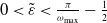 $0\lt \tilde \varepsilon \lt \frac {\pi }{\omega _{\textrm {max}}}-\frac 12$
and the penalty parameters
 $\gamma _e$
for
 $e\in \mathcal{E}^I$
are numbers with nonnegative imaginary parts, respectively. From Theorem2.4, the solution
 $u$
to the NLH problem (1.1)–(1.3) belongs to
 $H^{\frac 32+\tilde \varepsilon }(\Omega )$
, and hence
 $J(u,v)=0\ \forall v\in V.$
The CIPFEM for (2.1) reads: find
 $u_h\in V_{\mathcal{T}}$
such that
 \begin{equation} a^\gamma _{u_h}(u_h,v_h)= (f,v_h)+\langle g,v_h\rangle _{\Gamma _{\textrm {imp}}}\quad \forall v_h\in V_{\mathcal{T}}. \end{equation}
We remark that when
 $\gamma _e\equiv 0$
for all
 $e \in \mathcal{E}^I$
, the CIPFEM reduces to the standard FEM.
The corresponding auxiliary discrete problem and Newton’s iteration read as: find
 $w_{h}, u_h^{l+1}\in V_{\mathcal{T}}$
such that
 \begin{align} a^\gamma _0(w_{h},v_h)-k^2\varepsilon \big (2\big \vert \psi \big \vert ^2 w_{h}+\psi ^2\overline {w_{h}},v_h\big )_{\Omega _{0}}=(F,v_h)+\langle g,v_h\rangle _{\Gamma _{\textrm {imp}}}\quad \forall v_h\in V_{\mathcal{T}}, \end{align}
 \begin{align} a^\gamma _0(u^{l+1}_h,v_h)-k^2\varepsilon \big (2\big \vert u^l_h\big \vert ^2 u^{l+1}_h+(u^l_h)^2\overline {u^{l+1}_h},v_h\big )_{\Omega _{0}}=(f^l_h,v_h)+\langle g,v_h\rangle _{\Gamma _{\textrm {imp}}}\quad \forall v_h\in V_{\mathcal{T}}, \end{align}
where
 $f^l_h\,:\!=\,f-2k^2\varepsilon {\mathbf{1}}_{\Omega _{0}}\vert u^l_h\vert ^2u^l_h$
and
 $u_h^0\in V_{\mathcal{T}}$
. The other two iterations can be similarly constructed.
Next we introduce the Scott–Zhang interpolant
 $\mathcal I_h$
onto
 $V_{\mathcal{T}}$
[Reference Scott and Zhang44]. For any
 $v\in H^s(\Omega )$
,
 $s=1,2$
and the singular functions
 $S_j$
, the interpolation estimates in [Reference Scott and Zhang44, Theorem 4.1] and [Reference Chaumont-Frelet and Nicaise16, Lemma 5.1] are as follows:
 \begin{align} \begin{aligned} \|v-\mathcal I_h v\|_0 + h_{\mathcal{T}}\|v-\mathcal I_h v\|_1 + h_{\mathcal{T}}|\mathcal I_h v|_J &\lesssim h^s_{\mathcal{T}}|v|_s, \\ \left \Vert S_j-\mathcal I_hS_j\right \Vert _{0}+h_{\mathcal{T}}\left \Vert S_j-\mathcal I_hS_j\right \Vert _{1} + h_{\mathcal{T}}|\mathcal I_h S_j|_J &\lesssim h^{1+\alpha _j}_{\mathcal{T}},\quad j=1,2,\ldots ,N, \end{aligned} \end{align}
where
 $|\cdot |_J\,:\!=\,\big (\!\sum _{e\in \mathcal E^I}h_e\big \|[\![\nabla \cdot ]\!] \big \|^2_{0,e} \big )^{\frac 12}$
. For any
 $\phi \in H^1_{\Gamma _{\textrm {Dir}}}(\Omega )$
, its elliptic projection
 $P_h\phi \in V_{\mathcal{T}}$
is defined by
 \begin{align*} b(P_h\phi ,v_h)=b(\phi ,v_h)\ \ \forall v_h\in V_{\mathcal{T}}, \quad \text{where } b(u,v)\,:\!=\,(\nabla u,\nabla v)+(u,v). \end{align*}
Naturally, the following Galerkin orthogonality holds
 \begin{align} b(\phi -P_h\phi ,v_h)=0\quad \forall v_h\in V_{\mathcal{T}}, \end{align}
and we have the following projection error estimates (see, e.g., [Reference Duan and Wu21, Lemma 2.4]):
 \begin{align} h_{\mathcal{T}}^{-\alpha }\left \Vert \phi -P_h\phi \right \Vert _{0}+h_{\mathcal{T}}^{-\frac {\alpha }2}\left \Vert \phi -P_h\phi \right \Vert _{0,\Gamma _{\textrm {imp}}}\lesssim \left \Vert \phi -P_h\phi \right \Vert _{1}=\inf _{v_h\in V_{\mathcal{T}}}\left \Vert \phi -v_h\right \Vert _{1}\!, \end{align}
where
 $\alpha \,:\!=\,\frac {\pi }{\omega _{\textrm {max}}}=\min \limits _{1\leq j\leq N}\alpha _j$
. Since
 $b(u,v)$
is symmetric, it also holds that
 $b(v_h,P_h\phi )=b(v_h,\phi )\ \ \forall v_h\in V_{\mathcal{T}}$
, and the similar Galerkin orthogonality. In particular, we show the relationship between
 $a_\psi (\cdot ,\cdot )$
and
 $b(\cdot ,\cdot )$
for convenience,
 \begin{align} a_\psi (u,v)=b(u,v)-(k^2+1)(u,v)-k^2\varepsilon (\vert \psi \vert ^2u,v)_{\Omega _0}+\mathbf{i} k\langle u,v\rangle _{\Gamma _{\textrm {imp}}}. \end{align}
Let
 $b^\gamma (u,v)\,:\!=\,b(u,v)+J(u,v)$
. Similar to [Reference Du and Wu20, Lemma 6.3], by the local trace inequality, we find that there exists a constant
 $\gamma _1\gt 0$
such that if
 $\Re \gamma _e \geq -\gamma _1$
for any
 $e\in \mathcal E^I$
, then
 \begin{align} \Re b^\gamma (v_h,v_h)\geq \frac 12\|v_h\|_1^2 \quad \forall v_h\in V_{\mathcal{T}}. \end{align}
For simplicity, we assume that
 $\gamma _e\equiv \gamma$
for all
 $e\in \mathcal{E}^I$
in what follows, where
 $\gamma$
is a constant. The general case follows similarly. In the rest of the paper, we suppose that
 $\Re \gamma \geq -\gamma _1$
and
 $|\gamma |\lesssim 1$
.
Let
 \begin{align} t(k,h)\,:\!=\,k^{\frac 12}h^{\frac {\alpha }2}+k^{\frac 12+\alpha }h^\alpha +k^{\frac 32}h^{\frac {1+\alpha }2}+k^2h^{1+\frac {\alpha }2}+k^{\frac 32+\alpha }h^{2\alpha }+k^3h^{1+\alpha }. \end{align}
Noting that
 \begin{align*} t(k,h)&=k^{\frac {1-2\alpha }{2(1+\alpha )}}(k^3h^{1+\alpha })^{\frac {\alpha }{2(1+\alpha )}}+k^{\frac {(2\alpha -1)(\alpha -1)}{2(1+\alpha )}}(k^3h^{1+\alpha })^{\frac {\alpha }{1+\alpha }}+(k^3h^{1+\alpha })^{\frac 12}\\ &\quad +(kh)^{\frac 12}(k^{\frac 32}h^{\frac {1+\alpha }2})+k^{\frac {(2\alpha -1)(\alpha -3)}{2(1+\alpha )}}(k^3h^{1+\alpha })^{\frac {2\alpha }{1+\alpha }}+k^3h^{1+\alpha }, \end{align*}
we know that
 \begin{align} t(k,h)\lesssim 1 \quad \text{if}\quad k^3 h^{1+\alpha }\lesssim 1. \end{align}
Moreover,
 $t(k,h)$
is sufficiently small on condition that
 $k^3 h^{1+\alpha }$
is small enough.
The following lemma gives a stability estimate in energy norm and the interior stability estimate in
 $L^{\infty }$
norm for
 $w_h$
on locally refined meshes, which are discrete versions of the estimates in (2.4) for
 $w_\psi$
. Since the triangulation in the current case is only locally quasi-uniform, the proof of
 $L^{\infty }$
interior stability estimate in [Reference Wu and Zou47] is not valid.
Lemma 2.6.
Suppose
 $k\varepsilon \left \Vert \psi \right \Vert _{L^{\infty }(\Omega _{0})}^2\leq \theta _0$
and
 $k^3h_{\mathcal{T}}^{1+\alpha }\leq C_0$
, then the solution of (2.15) satisfies
 \begin{equation} \left\Vert {\hskip -4.1pt}\left\vert w_h \right\vert {\hskip -4.1pt}\right\Vert \lesssim M(F,g) \quad \mbox{and}\quad \left \Vert w_h\right \Vert _{L^{\infty }(\Omega _{0})}\lesssim \left \vert \ln h_{\mathcal{T},\mathrm {min}} \right \vert ^{\frac 12} k^{-\frac 12}\widehat {M}(F,g). \end{equation}
Proof. In this proof, we introduce a new elliptic projection
 $P_h^\gamma \colon V\mapsto V_{\mathcal{T}}$
(see, e.g., [Reference Du and Wu20, (6.9)]), defined by
 \begin{align*} b^\gamma (P_h^\gamma \phi , v_h)=b^\gamma (\phi ,v_h),\quad \forall v_h\in V_{\mathcal{T}},\; \phi \in V. \end{align*}
Similar to (2.19), the following estimate holds:
 \begin{align} h_{\mathcal{T}}^{-\alpha }\left \Vert \phi -P_h^\gamma \phi \right \Vert _{0}+h_{\mathcal{T}}^{-\frac {\alpha }2}\left \Vert \phi -P_h^\gamma \phi \right \Vert _{0,\Gamma _{\textrm {imp}}} \lesssim \|\phi -P_h^\gamma \phi \|_J \lesssim \inf _{v_h\in V_{\mathcal{T}}}\|\phi -v_h\|_J, \end{align}
where
 $\|\cdot \|_J\,:\!=\,\big (\|\cdot \|_1^2 + |\cdot |_J^2 \big )^{\frac 12}$
.
The proof of the first estimate in (2.24) is similar to that of [Reference Wu and Zou47, Lemma 3.2] with the help of (2.25) and (2.17) due to corner singularities. We prove it in the appendix.
Next we prove the second estimate. First, by using the singularity decomposition of
 $w_\psi$
in Lemma 2.2 and following the proof of [Reference Jiang, Li, Wu and Zou34, Lemma 4.1], which uses the modified duality argument and regards the second term in (2.15) as a small perturbation, we can derive the following error estimates in energy and
 $L^2$
norms by the new elliptic projection (see also [Reference Chaumont-Frelet and Nicaise16, Theorem 5.5], [Reference Wu46, Theorem 4.4]), under the condition that
 $\Re \gamma \geq -\gamma _1, |\gamma |\lesssim 1$
,
 $k\varepsilon \left \Vert \psi \right \Vert _{L^{\infty }(\Omega _{0})}^2\le \theta _0$
and
 $k^3h_{\mathcal{T}}^{1+\alpha }\le C_0$
, the details are omitted.
 \begin{align} \begin{split} \left\Vert {\hskip -4.1pt}\left\vert w_\psi -w_h \right\vert {\hskip -4.1pt}\right\Vert &\lesssim \big (kh_{\mathcal{T}}+k^{-\frac 12}(kh_{\mathcal{T}})^{\alpha }+k^3h_{\mathcal{T}}^2\big )\widehat {M}(F,g), \\ \left \Vert w_\psi -w_h\right \Vert _{0}&\lesssim \big (k^{-1}(kh_{\mathcal{T}})^{2\alpha }+k^2h_{\mathcal{T}}^2\big )\widehat {M}(F,g). \end{split} \end{align}
On the other hand, from [Reference Bramble and Xu10, Lemma 2.3], there holds
 \begin{align} \left \Vert w_h\right \Vert _{L^{\infty }(\Omega _{0})}\lesssim \left \vert \ln h_{\mathcal{T},\textrm {min}} \right \vert ^{\frac 12}\left \Vert w_h\right \Vert _{1,\Omega _{0}}\!. \end{align}
Indeed, the result there can be easily verified for the non-quasi-uniform meshes by replacing
 $\left \vert \ln h \right \vert ^{\frac 12}$
with
 $\left \vert \ln h_{\mathcal{T},\textrm {min}} \right \vert ^{\frac 12}$
.
To proceed, let
 $\zeta _h=w_h-P_h^\gamma w_\psi$
, then we have
 \begin{align} \left \Vert w_h\right \Vert _{L^{\infty }(\Omega _{0})}\leq \left\Vert w_\psi \right\Vert _{L^{\infty }(\Omega _{0})}+\left \Vert w_\psi -I_h w_\psi \right \Vert _{L^{\infty }(\Omega _{0})}+\left \Vert I_h w_\psi -P_h^\gamma w_\psi \right \Vert _{L^{\infty }(\Omega _{0})}+\left \Vert \zeta _h\right \Vert _{L^{\infty }(\Omega _{0})}\!, \end{align}
where
 $I_h$
is the standard FE interpolation operator. The first term can be estimated by directly using (2.4). Noting that
 $w_\psi |_{\Omega _{0}}=w_R|_{\Omega _{0}}$
since
 $w_\psi =w_{R}+\sum _{j=1}^N C_k^jS_j$
and the support of
 $S_j(1\leq j\leq N)$
does not intersect
 $\Omega _{0}$
, so the second term is estimated by using Lemma 2.2 and the interpolation error estimate
 $\left \Vert w_R-I_hw_R\right \Vert _{L^\infty (\Omega _{0})}\lesssim h_{\mathcal{T}}\left \vert w_R\right \vert _{2,\Omega _{0}}$
(see, e.g., [Reference Brenner and Scott11, (4.4.8)]):
 \begin{align} \begin{aligned} \left \Vert w_\psi -I_h w_\psi \right \Vert _{L^{\infty }(\Omega _{0})}&=\left \Vert w_R-I_h w_R\right \Vert _{L^{\infty }(\Omega _{0})}\lesssim kh_{\mathcal{T}}\widehat {M}(F,g)= k^{-\frac 12}(k^3h_{\mathcal{T}}^2)^{\frac 12}\widehat {M}(F,g). \end{aligned} \end{align}
To estimate the third term, we apply (2.27), (2.25), (2.17), the interpolation estimates, the local trace inequality and Lemma 2.2 to obtain
 \begin{align} \begin{aligned} \left \Vert I_h w_\psi -P_h^\gamma w_\psi \right \Vert _{L^{\infty }(\Omega _{0})} &\lesssim \left \vert \ln h_{\mathcal{T},\textrm {min}} \right \vert ^{\frac 12}\left \Vert I_h w_\psi -P_h^\gamma w_\psi \right \Vert _{1,\Omega _{0}}\\ &\lesssim \left \vert \ln h_{\mathcal{T},\textrm {min}} \right \vert ^{\frac 12}\big (\!\left \Vert w_R-I_h w_R\right \Vert _{1,\Omega _{0}}+\left \Vert w_\psi -P_h^\gamma w_\psi \right \Vert _{1}\!\big )\\ &\lesssim \left \vert \ln h_{\mathcal{T},\textrm {min}} \right \vert ^{\frac 12} \big ( \!\left \Vert w_R-I_h w_R\right \Vert _{1,\Omega _{0}} + \|w_\psi -\mathcal I_h w_\psi \|_J \big ) \\ &\lesssim \left \vert \ln h_{\mathcal{T},\textrm {min}} \right \vert ^{\frac 12} k^{-\frac 12}\big ((k^3h_{\mathcal{T}}^2)^{\frac 12}+(kh_{\mathcal{T}})^\alpha \big )\widehat {M}(F,g). \end{aligned} \end{align}
It remains to estimate
 $\left \Vert \zeta _h\right \Vert _{L^{\infty }(\Omega _{0})}$
. By simple calculations, we find
 \begin{align*} b^\gamma (\zeta _h,v_h) & =\big ((k^2+1+2k^2\varepsilon {\mathbf{1}}_{\Omega _{0}}\vert \psi \vert ^2)(w_h-w_\psi )+k^2\varepsilon {\mathbf{1}}_{\Omega _{0}}\psi ^2(\overline {w_h}-\overline {w_\psi }),v_h\big )\\& \quad +\mathbf{i} k\langle w_\psi -w_h,v_h\rangle _{\Gamma _{\textrm {imp}}} \ \ \forall v_h\in V_{\mathcal{T}}. \end{align*}
Then we define
 $\zeta \in H^1_{\Gamma _{\textrm {Dir}}}(\Omega )$
as the solution of the following variational problem:
 \begin{align} b(\zeta ,v) & =\big ((k^2+1+2k^2\varepsilon {\mathbf{1}}_{\Omega _{0}}\vert \psi \vert ^2)(w_h-w_\psi )+k^2\varepsilon {\mathbf{1}}_{\Omega _{0}}\psi ^2(\overline {w_h}-\overline {w_\psi }),v\big )\nonumber\\ & \quad +\mathbf{i} k\langle w_\psi -w_h,v\rangle _{\Gamma _{\textrm {imp}}} \ \ \forall v\in H^1_{\Gamma _{\textrm {Dir}}}(\Omega ). \end{align}
It is clear that
 $\zeta _h=P_h^{\gamma } \zeta$
. By the singularity decomposition of the elliptic equations in [Reference Grisvard27], we derive
 $\zeta =\zeta _R+\sum _{j=1}^Nc_jS_j$
, and
 \begin{align} \begin{aligned} \left \Vert \zeta _R\right \Vert _{2}+\sum _{j=1}^N\left \vert c_j \right \vert &\lesssim \big \Vert (k^2+1+k^2\varepsilon {\mathbf{1}}_{\Omega _{0}}\vert \psi \vert ^2)(w_\psi -w_h)\big \Vert _0+k\left \Vert w_\psi -w_h\right \Vert _{\frac 12,\Gamma _{\textrm {imp}}}\\ &\lesssim \big (k^2(k^{-1}(kh_{\mathcal{T}})^{2\alpha }+k^2h^2_{\mathcal{T}})+k(kh_{\mathcal{T}}+k^{-\frac 12}(kh_{\mathcal{T}})^{\alpha }+k^3h^2_{\mathcal{T}})\big )\widehat {M}(F,g)\\ &\lesssim (k^4h^2_{\mathcal{T}}+k^2h_{\mathcal{T}}+k^{\frac 12}(kh_{\mathcal{T}})^{\alpha })\widehat {M}(F,g), \end{aligned} \end{align}
where we use (2.26) and the trace inequality. Then, taking (2.32) into (2.25) and using (2.17), we have
 \begin{align} \left \Vert \zeta -\zeta _h\right \Vert _{0}+h_{\mathcal{T}}^{\alpha }\!\left \Vert \zeta -\zeta _h\right \Vert _{1}\lesssim h^{2\alpha }_{\mathcal{T}}(k^4h^2_{\mathcal{T}}+k^2h_{\mathcal{T}}+k^{\frac 12}(kh_{\mathcal{T}})^{\alpha })\widehat {M}(F,g). \end{align}
Like the analyses in (2.29) and (2.30), we get
 \begin{align} \begin{aligned} \left \Vert \zeta -\zeta _h\right \Vert _{L^{\infty }(\Omega _{0})}&\lesssim \left \Vert \zeta -I_h \zeta \right \Vert _{L^{\infty }(\Omega _{0})}+\left \Vert \zeta _h-I_h\zeta \right \Vert _{L^{\infty }(\Omega _{0})}\\ &\lesssim h_{\mathcal{T}}\left \vert \zeta _R\right \vert _{2}+\left \vert \ln h_{\mathcal{T},\textrm {min}} \right \vert ^{\frac 12}\big (\|\zeta -I_h \zeta \|_{1,\Omega _{0}} + \left \Vert \zeta -\zeta _h\right \Vert _{1}\!\big )\\ &\lesssim h_{\mathcal{T}}\left \vert \zeta _R\right \vert _{2}+\left \vert \ln h_{\mathcal{T},\textrm {min}} \right \vert ^{\frac 12} \big ( h_{\mathcal{T}}\left \vert \zeta _R\right \vert _{2} + \left \Vert \zeta - \zeta _h\right \Vert _{1} \!\big )\\ &\lesssim h^{\alpha }_{\mathcal{T}}(k^4h^2_{\mathcal{T}}+k^2h_{\mathcal{T}}+k^{\frac 12}(kh_{\mathcal{T}})^{\alpha })(1+\left \vert \ln h_{\mathcal{T},\textrm {min}} \right \vert ^{\frac 12}\!)\widehat {M}(F,g)\\ &\le k^{-\frac 12}\big (k^{\frac {3}{2}} h_{\mathcal{T}}+2k^{-\frac 12}\big )t(k,h_{\mathcal{T}})(1+\left \vert \ln h_{\mathcal{T},\textrm {min}} \right \vert ^{\frac 12}\!)\widehat {M}(F,g). \end{aligned} \end{align}
After rewriting (2.31) as:
 \begin{align*} a_{0}(\zeta ,v)-k^2\varepsilon \big (2\left \vert \psi \right \vert ^2\zeta +\psi ^2\bar \zeta ,v\big )_{\Omega _{0}}&= \big ((k^2+1+2k^2\varepsilon {\mathbf{1}}_{\Omega _{0}}\vert \psi \vert ^2)(P_h^\gamma w_\psi - w_{\psi } + \zeta _h - \zeta ),v\big )\\ &\quad +k^2\varepsilon \big (\vert \psi \vert ^2\overline {(P_h^\gamma w_\psi -w_{\psi }+\zeta _h-\zeta )},v\big )_{\Omega _{0}}\\ &\quad +\mathbf{i} k\langle w_{\psi } - P_h^\gamma w_{\psi }+\zeta -\zeta _h,v\rangle _{\Gamma _{\textrm {imp}}} \quad \forall v\in H^1_{\Gamma _{\textrm {Dir}}}(\Omega ), \end{align*}
it follows from Lemma 2.2, (2.25), (2.33), the trace inequality, and the condition
 $k^3h_{\mathcal{T}}^{1+\alpha }\leq C_0$
that
 \begin{align} \begin{aligned} \left \Vert \zeta \right \Vert _{L^{\infty }(\Omega _{0})}&\lesssim k^{-\frac 12}\big (k^2\!\left \Vert P_h^\gamma w_\psi - w_{\psi } + \zeta _h - \zeta \right \Vert _{0}+k\!\left \Vert P_h^\gamma w_\psi - w_{\psi } + \zeta _h - \zeta \right \Vert _{0,\Gamma _{\textrm {imp}}}\!\big )\\ &\lesssim k^{-\frac 12}\big (k^2h_{\mathcal{T}}^\alpha (kh_{\mathcal{T}}+k^{-\frac 12}(kh_{\mathcal{T}})^\alpha )+k^2h^{2\alpha }_{\mathcal{T}}(k^4h^2_{\mathcal{T}}+k^2h_{\mathcal{T}}+k^{\frac 12}(kh_{\mathcal{T}})^{\alpha })\\ &\quad +kh_{\mathcal{T}}^{\frac {\alpha }2}(kh_{\mathcal{T}}+k^{-\frac 12}(kh_{\mathcal{T}})^\alpha )+kh^{\frac {3\alpha }2}_{\mathcal{T}}(k^4h^2_{\mathcal{T}}+k^2h_{\mathcal{T}}+k^{\frac 12}(kh_{\mathcal{T}})^{\alpha })\big )\widehat {M}(F,g)\\ & \lesssim k^{-\frac 12}\big (t(k,h_{\mathcal{T}})+t^2(k,h_{\mathcal{T}})\big )\widehat {M}(F,g). \end{aligned} \end{align}
Finally, the result comes from combining (2.28), (2.4), (2.29), (2.34), (2.35), (2.23), and the fact
 $\frac 12\lt \alpha \le 1$
.
Then for the Newton’s iterative sequences
 $\{u_h^l\}$
, we argue as in the proof of Lemma 2.3 to have
Lemma 2.7.
If
 $k\varepsilon \left \Vert u_h^0\right \Vert _{L^{\infty }(\Omega _{0})}^2\leq \left \vert \ln h_{\mathcal{T},\mathrm {min}} \right \vert \varepsilon \widehat {M}(f,g)^2\leq \theta _0$
and
 $k^3h_{\mathcal{T}}^{1+\alpha }\leq C_0$
, then
 \begin{equation*} \left\Vert {\hskip -4.1pt}\left\vert u_h^l \right\vert {\hskip -4.1pt}\right\Vert \lesssim M(f,g) \quad \mbox{and}\quad \left \Vert u_h^l\right \Vert _{L^{\infty }(\Omega _{0})}\lesssim \left \vert \ln h_{\mathcal{T},\mathrm {min}} \right \vert ^{\frac 12} k^{-\frac 12}\widehat {M}(f,g) \quad \mbox{for} \,\,l=1,2,\ldots \end{equation*}
Using the convergence of the iteration sequence, we can get:
Theorem 2.8.
If
 $\left \vert \ln h_{\mathcal{T},\mathrm {min}} \right \vert \varepsilon \widehat {M}(f,g)^2\leq \theta _0$
and
 $k^3h_{\mathcal{T}}^{1+\alpha }\leq C_0$
, then (2.14) attains a unique solution
 $u_h$
satisfying the following stability estimates
 \begin{align} \left\Vert {\hskip -4.1pt}\left\vert u_h \right\vert {\hskip -4.1pt}\right\Vert \lesssim M(f,g) \quad \mbox{and}\quad \left \Vert u_h\right \Vert _{L^{\infty }(\Omega _{0})}\lesssim \left \vert \ln h_{\mathcal{T},\mathrm {min}} \right \vert ^{\frac 12} k^{-\frac 12}\widehat {M}(f,g). \end{align}
Moreover, there holds the error estimates
 \begin{align} \begin{aligned} \left\Vert {\hskip -4.1pt}\left\vert u-u_h \right\vert {\hskip -4.1pt}\right\Vert &\lesssim (kh_{\mathcal{T}}+k^{-\frac 12}(kh_{\mathcal{T}})^{\alpha }+k^3h_{\mathcal{T}}^2)\widehat {M}(f,g),\\ k\left \Vert u-u_h\right \Vert _{0}&\lesssim \big ((kh_{\mathcal{T}})^{2\alpha }+k^3h_{\mathcal{T}}^2\big )\widehat {M}(f,g). \end{aligned} \end{align}
Proof. (2.36) can be directly obtained from the convergence of iteration methods, which can be proved by following the proof of Theorem2.4. We omit the details for simplicity. The proof of (2.37) is a little more complex, but it is still based on the convergences of
 $\{u^l\}$
and
 $\{u^l_h\}$
.
We define
 $\hat u_h^0=u_h^0$
and
 $\hat u_h^l\in V_{\mathcal{T}} (l=1,2,\ldots )$
to be the solution to the following problem
 \begin{align*} a_0^\gamma (\hat u^l_h, v_h)-k^2\varepsilon \big (2\left \vert u^{l-1} \right \vert ^2\hat u^l_h+(u^{l-1})^2\overline {\hat u^l_h},v_h\big )_{\Omega _{0}}=(f^{l-1}, v_h)+\langle g, v_h\rangle _{\Gamma _{\textrm {imp}}}\quad \forall v_h\in V_{\mathcal{T}}. \end{align*}
Then, from (2.26) and (2.11), we have
 \begin{align} \begin{aligned} \left\Vert {\hskip -4.1pt}\left\vert u^l-\hat u^l_h \right\vert {\hskip -4.1pt}\right\Vert &\lesssim (kh_{\mathcal{T}}+k^{-\frac 12}(kh_{\mathcal{T}})^{\alpha }+k^3h_{\mathcal{T}}^2)\widehat {M}(f,g),\\ k\left \Vert u^l-\hat u^l_h\right \Vert _{0}&\lesssim \big ((kh_{\mathcal{T}})^{2\alpha }+k^3h_{\mathcal{T}}^2\big )\widehat {M}(f,g). \end{aligned} \end{align}
Next we need to estimate
 $\hat \eta ^l_h\,:\!=\,\hat u^l_h-u^l_h$
. Through simple calculation, we find
 $\hat \eta _h^l$
satisfies
 \begin{align*} a_0^\gamma (\hat \eta _h^l,v_h)-k^2\varepsilon \big (2\left \vert u^{l-1} \right \vert ^2\hat \eta _h^l+(u^{l-1})^2\overline {\hat \eta _h^l},v_h\big )_{\Omega _{0}}&=k^2\varepsilon \big (2\big (\!\left \vert u^{l-1} \right \vert ^2-\left \vert u^{l-1}_h \right \vert ^2\big )u^l_h+\big ((u^{l-1})^2-(u^{l-1}_h)^2\big )\overline {u^l_h},v_h\big )_{\Omega _{0}}\\ &\quad + 2k^2\varepsilon \big (\!\left \vert u^{l-1}_h \right \vert ^2u^{l-1}_h-\left \vert u^{l-1} \right \vert ^2u^{l-1},v_h\big )_{\Omega _{0}}\qquad \forall v_h\in V_{\mathcal{T}}. \end{align*}
It is shown from Lemmas 2.6, 2.3, and 2.7 that
 \begin{align*} \left\Vert {\hskip -4.1pt}\left\vert \hat \eta ^l_h \right\vert {\hskip -4.1pt}\right\Vert &\lesssim k^2\varepsilon \left \Vert \big (\!\left \vert u^{l-1} \right \vert ^2-\left \vert u^{l-1}_h \right \vert ^2\!\big )(u^l_h-u^{l-1}_h)+\big ((u^{l-1})^2-(u^{l-1}_h)^2\big )\overline {u^l_h}+\left \vert u^{l-1} \right \vert ^2(u^{l-1}_h-u^{l-1})\right \Vert _{0,\Omega _{0}}\\ &\lesssim k\varepsilon \left \vert \ln h_{\mathcal{T},\textrm {min}} \right \vert \widehat {M}(f,g)^2\left \Vert u^{l-1}-u^{l-1}_h\right \Vert _{0}. \end{align*}
So when
 $\varepsilon \left \vert \ln h_{\mathcal{T},\textrm {min}} \right \vert \widehat {M}(f,g)^2$
is sufficiently small, we have
 \begin{align*} \left\Vert {\hskip -4.1pt}\left\vert \hat \eta ^l_h \right\vert {\hskip -4.1pt}\right\Vert \leq \frac 12\left\Vert {\hskip -4.1pt}\left\vert u^{l-1}-\hat u^{l-1}_h \right\vert {\hskip -4.1pt}\right\Vert +\frac 12\left\Vert {\hskip -4.1pt}\left\vert \hat \eta ^{l-1}_h \right\vert {\hskip -4.1pt}\right\Vert \quad \mbox{and}\quad \left \Vert \hat \eta ^l_h\right \Vert _{0}\leq \frac 12\left \Vert u^{l-1}-\hat u^{l-1}_h\right \Vert _{0}+\frac 12\left \Vert \hat \eta ^{l-1}_h\right \Vert _{0}\!, \end{align*}
and then
 \begin{align} \left\Vert {\hskip -4.1pt}\left\vert \hat \eta ^l_h \right\vert {\hskip -4.1pt}\right\Vert \leq \sum _{j=0}^{l-1}2^{j-l}\left\Vert {\hskip -4.1pt}\left\vert u^j-\hat u^j_h \right\vert {\hskip -4.1pt}\right\Vert \lesssim (kh_{\mathcal{T}}+k^{-\frac 12}(kh_{\mathcal{T}})^{\alpha }+k^3h_{\mathcal{T}}^2)\widehat {M}(f,g)+2^{-l}\left\Vert {\hskip -4.1pt}\left\vert u^0-u^0_h \right\vert {\hskip -4.1pt}\right\Vert . \end{align}
Combining (2.38) and (2.39), we derive
 \begin{align*} \left\Vert {\hskip -4.1pt}\left\vert u^l-u^l_h \right\vert {\hskip -4.1pt}\right\Vert \lesssim (kh_{\mathcal{T}}+k^{-\frac 12}(kh_{\mathcal{T}})^{\alpha }+k^3h_{\mathcal{T}}^2)\widehat {M}(f,g)+2^{-l}\left\Vert {\hskip -4.1pt}\left\vert u^0-u^0_h \right\vert {\hskip -4.1pt}\right\Vert . \end{align*}
Similarly,
 \begin{align*} k\left \Vert u^l-u^l_h\right \Vert _{0}\lesssim \big ((kh_{\mathcal{T}})^{2\alpha }+k^3h_{\mathcal{T}}^2\big )\widehat {M}(f,g)+2^{-l}\left \Vert u^0-u^0_h\right \Vert _{0}\!. \end{align*}
Then, (2.37) comes from letting
 $l\rightarrow \infty$
in the above two estimates. This completes the proof of the theorem.
Remark 2.9. (i) Denote by
 $\mathcal{T}_0$
the initial mesh.
 $\vert \ln h_{\mathcal{T},\mathrm {min}} \vert / \vert \ln h_{\mathcal{T}_0} \vert \eqsim$
the maximum number of times the mesh is refined locally, that is to say, although the condition here is more stringent than the one in [
Reference Jiang, Li, Wu and Zou34
] (
 $\varepsilon \widehat {M}(f,g)^2\leq \theta _0$
for the impedance boundary condition), it is also acceptable. In addition, to the best of our knowledge, little is known about an
 $L^{\infty }$
interior estimate of
 $u_h$
for the NLH problem on a shape regular mesh, especially a locally refined mesh. Moreover, another technique for analyzing the case of a shape regular mesh is directly using the
 $H^{1}$
global estimate instead of the
 $L^{\infty }$
interior estimate and requires more stringent conditions (see, e.g. [
Reference Maier and Verfürth38
]).
(ii) Similar to Remark 2.5 (i), Theorem
2.8
states that if
 $\left \vert \ln h_{\mathcal{T},\mathrm {min}} \right \vert \varepsilon \widehat {M}(f,g)^2\leq \theta _0$
and
 $k^3h_{\mathcal{T}}^{1+\alpha }\leq C_0$
, CIPFEM (2.14) attains a unique low-energy solution
 $u_h$
and
 $u_h$
approximates the low-energy solution
 $u$
to the NLH problem (2.1). Like the proof in [
Reference Jiang, Li, Wu and Zou34
], we can prove the local quadratic convergence of Newton’s iteration (2.16), which also holds for the high-energy solutions. The details are omitted.
3. A posteriori error estimates
In this section, we derive upper and lower bounds for the (CIP)FEM and the elliptic projection and establish some equivalent relationships between them which are of significance for proving the convergence and quasi-optimality.
3.1. Error estimators
We define
 $\Sigma _{\mathcal{T}}(T)\,:\!=\,\{T\}\cup\{T^{'}{\kern-1pt}\in \mathcal{T}\,:\,T^{'}\cap T\in \mathcal{E}\}$
to be the set of element
 $T$
and all other elements that have a common edge with
 $T$
, and let
 $\Omega _{\mathcal{T}}(T)\,:\!=\,\bigcup _{T'\in \Sigma _{\mathcal{T}}(T)}T'$
. For any
 $v_h\in V_{\mathcal{T}}$
, the element residuals, jump residuals, error estimators and oscillations for
 $v_h$
regarded as an approximation to the NLH problem (1.1)–(1.3) are defined as follows:
 \begin{align*} \begin{aligned} R_T(v_h)&\,:\!=\,\big (f+k^2(1+\varepsilon {\mathbf{1}}_{\Omega _{0}}\left \vert v_h \right \vert ^2\!)v_h\big )|_T,\ T\in \mathcal{T},\\ R_e(v_h)&\,:\!=\,\begin{cases} -\frac 12[\![\nabla v_h]\!], & e\subset \Omega ,\\ -\frac {\partial v_h}{\partial n}-\mathrm ikv_h+g, & e\subset \Gamma _{\textrm {imp}},\\ 0, & e\subset \Gamma _{\textrm {Dir}}, \end{cases} \quad R_{\partial T}|_e\,:\!=\,R_e,\ \forall e\subset \partial T,\\ \eta _T^2(v_h)&\,:\!=\,\sum _{T'\in \Sigma _{\mathcal{T}}(T)}h_{T'}^2\left \Vert R_{T'}(v_h)\right \Vert _{0,T'}^2+h_T\left \Vert R_{\partial T}(v_h)\right \Vert _{0,\partial T}^2,\\ \textrm {osc}_T^2(v_h)&\,:\!=\,h_{T}^2\big \Vert R_{T}(v_h)-\overline {\overline { R_{T}(v_h)}}\big \Vert _{0,T}^2+h_T\big \Vert R_{\partial T}(v_h)- \overline {\overline {R_{\partial T}(v_h)}}\big \Vert _{0,{\partial T}}^2\\ &=h_{T}^2\big \Vert f-\overline {\overline {f}}\big \Vert _{0,T}^2+h_T\!\left \Vert g- \overline {\overline {g}}\right \Vert _{0,{\partial T}\cap \Gamma _{\textrm {imp}}}^2\!, \end{aligned} \end{align*}
where
 $\overline {\overline {v}}|_T$
is the
 $L^2(T)$
projection of
 $v|_T$
onto
 $P_{3}(T)$
, and
 $\overline {\overline { v}}|_e$
is the
 $L^2(e)$
projection of
 $v|_e$
onto
 $P_{1}(e)$
.
The elliptic projection
 $P_hu$
for the solution
 $u$
of (2.1) can be seen as the FE discretization of the elliptic problem:
 \begin{align*} \left \{\!\begin{aligned} -\Delta \tilde u+\tilde u&=f+\big (k^2(1+\varepsilon {\mathbf{1}}_{\Omega _{0}}\vert u \vert ^2)+1\big )u \ \ \text{in} \ \Omega , \\ \frac {\partial \tilde u}{\partial n}&=-\mathrm iku+g \ \ \text{on} \ \Gamma _{\textrm {imp}};\quad \tilde u=0 \ \ \text{on} \ \Gamma _{\textrm {Dir}}. \end{aligned}\right . \end{align*}
Thus, the corresponding error estimators for
 $v_h$
can be stated:
 \begin{align} \begin{aligned} \widetilde R_T(v_h)&\,:\!=\,{\big (f+\big (k^2(1+\varepsilon {\mathbf{1}}_{\Omega _{0}}\vert u \vert ^2)+1\big )u-v_h\big )|}_T,\ T\in \mathcal{T},\\ \widetilde R_e(v_h)&\,:\!=\,{\begin{cases} -\frac 12[\![\nabla v_h]\!], & e\subset \Omega ,\\[3pt] -\frac {\partial v_h}{\partial n}-\mathrm iku+g, & e\subset \Gamma _{\textrm {imp}},\\ 0, &e\subset \Gamma _{\textrm {Dir}} \end{cases}} \quad \widetilde R_{\partial T}|_e\,:\!=\,\widetilde R_e,\ \forall e\subset \partial T,\\ \widetilde \eta _T^2(v_h)&\,:\!=\,\sum _{T'\in \Sigma _{\mathcal{T}}(T)}h_{T'}^2{\big \Vert \widetilde {R}_{T'}(v_h)\big \Vert }_{0,T'}^2+h_T\big \Vert \widetilde {R}_{\partial T}(v_h)\big \Vert _{0,\partial T}^2,\\ \widetilde {\textrm {osc}}_T^2(v_h)&\,:\!=\,h_{T}^2{\big \Vert \widetilde R_{T}(v_h)-\overline {\overline {\widetilde R_{T}(v_h)}}\big \Vert }_{0,T}^2+h_T{\big \Vert \widetilde R_{\partial T}(v_h)- \overline {\overline {\widetilde R_{\partial T}(v_h)}}\big \Vert }_{0,\partial T}^2. \end{aligned} \end{align}
For any submesh
 $\mathcal{M}\subset$
of
 $\mathcal{T}$
, we denote
 $\widetilde u_h\,:\!=\,P_hu$
, and
 \begin{align*} &R_T\,:\!=\,R_T(u_h),\ R_e\,:\!=\,R_e(u_h),\ \eta _T\,:\!=\,\eta _T(u_h),\ \textrm {osc}_T\,:\!=\,\textrm {osc}_T(u_h),\\ &\eta _{\mathcal{M}}\,:\!=\,\Big (\!\sum _{T\in \mathcal{M}}\eta _T^2\Big )^{\frac 12},\ \textrm {osc}_{\mathcal{M}}\,:\!=\,\Big (\!\sum _{T\in \mathcal{M}}\textrm {osc}_T^2\Big )^{\frac 12}, \end{align*}
Similarly, we omit the variables in the brackets in (3.1) when
 $v_h=\widetilde u_h$
and also for
 $\widetilde \eta _{\mathcal{M}}$
and
 $\widetilde {\textrm {osc}}_{\mathcal{M}}$
.
Remark 3.1. (i) Our error estimator
 $\eta _T$
on an element
 $T$
is slightly different from the standard residual-type error estimator defined as
 $\eta _T^{\mathrm {std}}\,:\!=\,\big (h_T^2\!\left \Vert R_{T}\right \Vert _{0,T}^2+h_T\left \Vert R_{\partial T}\right \Vert _{0,\partial T}^2\!\big )^{\frac {1}{2}}$
, but, apparently, their corresponding error estimators on the whole mesh are equivalent, that is,
 $\eta _{\mathcal{T}}\eqsim \eta _{\mathcal{T}}^{\mathrm {std}}$
. We introduce this new error estimator for the purpose of proving the convergence and quasi-optimality of the standard adaptive algorithm.
(ii) The auxiliary error estimators
 $\widetilde {\eta }_T$
associated with the elliptic projection are introduced only for the theoretical analysis and will not be used in the adaptive algorithm.
In the subsequent part of this paper, we consider the solutions
 $u$
and
 $u_h$
to (2.1) and (2.14) from Theorems2.4 and 2.8. In other words, we specifically take the case of low energy into account, namely we make the assumption.
Assumption 3.2.
Let
 $u$
and
 $u_h$
be the solutions to (2.1) and (2.14) from Theorem
2.4
and Theorem
2.8
, respectively.
The following lemma gives an estimate for the penalty term.
Lemma 3.3.
For any
 $\phi \in H^1_{\Gamma _{\mathrm {Dir}}}(\Omega )$
, the following estimate holds:
 \begin{align} |J(u_h,\mathcal I_h\phi )| + |J(u_h,P_h \phi )|\lesssim |\gamma | \eta _{\mathcal{T}} \|\nabla \phi \|_0. \end{align}
Proof. It follows from the local trace inequality and (2.17) that
 \begin{align*} \left \vert J(u_h,\mathcal I_h\phi ) \right \vert &\lesssim |\gamma |\sum _{e\in \mathcal E^I}h_e\big \|[\![\nabla u_h]\!]\big \|_{0,e}\big \|[\![\nabla \mathcal I_h\phi ]\!]\big \|_{0,e}\\ &\lesssim |\gamma |\eta _{\mathcal{T}}\|\nabla \mathcal I_h\phi \|_0 \lesssim |\gamma |\eta _{\mathcal{T}}\|\nabla \phi \|_0. \end{align*}
The proof of the estimate for
 $|J(u_h,P_h \phi )|$
is analogous and is therefore omitted.
3.2. Upper and lower bounds
We give a posteriori upper and lower bounds for the errors of
 $u_h$
and
 $P_hu$
in this subsection.
Theorem 3.4 (upper bounds). If
 $\vert \ln h_{\mathcal{T},\mathrm {min}} \vert \varepsilon \widehat {M}(f,g)^2\leq \theta _0\ \mbox{and}\ k^3h_{\mathcal{T}}^{1+\alpha }\leq C_0$
, then we have the estimates:
 \begin{align} \left \Vert \nabla (u-u_h)\right \Vert _{0}&\lesssim (1+k^2h_{\mathcal{T}})\eta _{\mathcal{T}},\\[-15pt]\nonumber \end{align}
 \begin{align} \left \Vert u-u_h\right \Vert _{0}&\lesssim \big (kh_{\mathcal{T}}+k^{-\frac 12}(kh_{\mathcal{T}})^\alpha \big )\eta _{\mathcal{T}},\\[-15pt]\nonumber \end{align}
 \begin{align} \left \Vert u-u_h\right \Vert _{0,\Gamma _{\mathrm {imp}}}&\lesssim \big (h_{\mathcal{T}}^{\frac {\alpha }2}+k^{\frac 12}h_{\mathcal{T}}^{\frac 12}+(k^{-\frac 12} +k^{\frac 12}h_{\mathcal{T}}^{\frac 12})|\gamma | \big )\eta _{\mathcal{T}},\\[-13pt]\nonumber \end{align}
 \begin{align} \left \Vert u-P_h u\right \Vert _{1}&\lesssim \eta _{\mathcal{T}},\\[-13pt]\nonumber \end{align}
 \begin{align} \left \Vert u-P_h u\right \Vert _{1}&\lesssim \widetilde \eta _{\mathcal{T}}. \end{align}
Proof. Denote by
 $e\,:\!=\,u-u_h$
,
 $\rho \,:\!=\,u-P_hu$
, and
 $\zeta _h\,:\!=\,P_hu-u_h$
. We show the following identity, which we will often use subsequently: for any
 $\phi \in H^1_{\Gamma _{\textrm {Dir}}}(\Omega )$
and
 $v_h\in V_{\mathcal{T}}$
,
 \begin{align} a_{u}(e,\phi )=\sum _{T\in \mathcal{T}}\big ((R_T,\phi -v_h)_T+\langle R_{\partial T},\phi -v_h\rangle _{\partial T}\big ) +J(u_h,v_h)+k^2\varepsilon \big ((\vert u \vert ^2-\left \vert u_h \right \vert ^2\!)u_h,\phi \big )_{\Omega _{0}}. \end{align}
Indeed, with the aid of elementwise integration by parts and
 $a_u(u,v_h)-a_{u_h}^\gamma (u_h,v_h)=0$
by (2.1), (2.14), we derive
 \begin{align*} a_{u}(e,\phi )&=a_{u}(u,\phi -v_h)-a_{u_h}(u_h,\phi -v_h) +J(u_h,v_h) +\big (a_{u_h}(u_h,\phi )-a_u(u_h,\phi )\big )\\ &=\big (f+k^2(1+\varepsilon {\mathbf{1}}_{\Omega _{0}}\left \vert u_h \right \vert ^2\!)u_h,\phi -v_h\big )+\langle g,\phi -v_h\rangle _{\Gamma _{\textrm {imp}}}-\mathbf{i} k\langle u_h,\phi -v_h\rangle _{\Gamma _{\textrm {imp}}}\\ & \quad \; -\sum _{T\in \mathcal{T}}\left\langle \frac {\partial u_h}{\partial n},\phi -v_h\right\rangle _{\partial T} +J(u_h,v_h) +k^2\varepsilon \big ((\vert u \vert ^2-\left \vert u_h \right \vert ^2\!)u_h,\phi \big )_{\Omega _{0}}\\ &=\sum _{T\in \mathcal{T}}\big ((R_T,\phi -v_h)_T+\langle R_{\partial T},\phi -v_h\rangle _{\partial T}\big )+J(u_h,v_h) +k^2\varepsilon \big ((\vert u \vert ^2-\left \vert u_h \right \vert ^2\!)u_h,\phi \big )_{\Omega _{0}}. \end{align*}
First, we estimate
 $\zeta _h$
. Taking
 $\phi =v_h=\zeta _h$
in (3.8), and using (2.20) and (2.18), we have
 \begin{align} a_u(\zeta _h,\zeta _h)&=a_u(e,\zeta _h)-a_u(\rho ,\zeta _h)\notag \\ &=k^2\varepsilon \big ((\vert u \vert ^2-\left \vert u_h \right \vert ^2\!)u_h+\left \vert u \right \vert ^2\rho ,\zeta _h\big )_{\Omega _{0}}+J(u_h,\zeta _h) +(k^2+1)(\rho ,\zeta _h)-\mathbf{i} k\langle \rho ,\zeta _h\rangle _{\Gamma _{\textrm {imp}}}. \end{align}
Taking the imaginary part of (3.9) and noting
 $e = \rho + \zeta _h$
, by
 $L^\infty$
interior estimates in (2.12) and (2.36), we have
 \begin{align*} \begin{aligned} k\left \Vert \zeta _h\right \Vert ^2_{0,\Gamma _{\textrm {imp}}}&\lesssim k\theta _0(\!\left \Vert e\right \Vert _{0}+\Vert \rho \Vert _{0})\left \Vert \zeta _h\right \Vert _{0}+k^2h_{\mathcal{T}}^\alpha \Vert \rho \Vert _{1}\left \Vert \zeta _h\right \Vert _{0}+k^{\frac 12}h_{\mathcal{T}}^{\frac {\alpha }2}\Vert \rho \Vert _{1}k^{\frac 12}\left \Vert \zeta _h\right \Vert _{0,\Gamma _{\textrm {imp}}} +|\gamma |\eta _{\mathcal{T}} \|\nabla \zeta _h\|_0 \\ &\lesssim k \left \Vert \zeta _h\right \Vert _{0}^2 +k^2h_{\mathcal{T}}^\alpha \Vert \rho \Vert _{1}\left \Vert \zeta _h\right \Vert _{0}+k^{\frac 12}h_{\mathcal{T}}^{\frac {\alpha }2}\Vert \rho \Vert _{1}k^{\frac 12}\left \Vert \zeta _h\right \Vert _{0,\Gamma _{\textrm {imp}}} +|\gamma |\eta _{\mathcal{T}} \|\nabla \zeta _h\|_0 \end{aligned} \end{align*}
where (2.19) and the local trace inequality are also used. Then, by Young’s inequality, we proceed
 \begin{align*} k\left \Vert \zeta _h\right \Vert _{0,\Gamma _{\textrm {imp}}}^2\lesssim (k+k^3h_{\mathcal{T}}^{\alpha })\left \Vert \zeta _h\right \Vert _{0}^2+kh_{\mathcal{T}}^\alpha \Vert \rho \Vert _{1}^2 +|\gamma |\eta _{\mathcal{T}} \|\nabla \zeta _h\|_0, \end{align*}
which means
 \begin{align} \left \Vert \zeta _h\right \Vert _{0,\Gamma _{\textrm {imp}}}\lesssim (1+kh_{\mathcal{T}}^{\frac {\alpha }2})\left \Vert \zeta _h\right \Vert _{0}+h_{\mathcal{T}}^{\frac {\alpha }2}\Vert \rho \Vert _{1} +k^{-\frac 12}|\gamma |^{\frac 12}\eta _{\mathcal{T}}^{\frac 12} \|\nabla \zeta _h\|_0^{\frac 12}. \end{align}
Taking the real part of (3.9), we have the following inequalities by using (2.19) and (3.10)
 \begin{align*} \left \Vert \nabla \zeta _h\right \Vert _{0}^2&\lesssim (k^2+\theta _0 k)\left \Vert \zeta _h\right \Vert _{0}^2+k\theta _0 h_{\mathcal{T}}^\alpha \Vert \rho \Vert _{1}\left \Vert \zeta _h\right \Vert _{0}+k^2h_{\mathcal{T}}^\alpha \Vert \rho \Vert _{1}\left \Vert \zeta _h\right \Vert _{0}+kh^{\frac {\alpha }2}_{\mathcal{T}}\Vert \rho \Vert _{1}\left \Vert \zeta _h\right \Vert _{0,\Gamma _{\textrm {imp}}} +|\gamma |\eta _{\mathcal{T}} \|\nabla \zeta _h\|_0 \\ &\lesssim k^2\left \Vert \zeta _h\right \Vert _{0}^2+(kh^{\frac {\alpha }2}_{\mathcal{T}}+k^2h_{\mathcal{T}}^\alpha )\Vert \rho \Vert _{1}\left \Vert \zeta _h\right \Vert _{0}+kh_{\mathcal{T}}^\alpha \Vert \rho \Vert _{1}^2 +|\gamma |^{\frac 12}k^{\frac 12}h^{\frac {\alpha }2}_{\mathcal{T}}\|\rho \|_1\eta _{\mathcal{T}}^{\frac 12} \|\nabla \zeta _h\|_0^{\frac 12} +|\gamma |\eta _{\mathcal{T}} \|\nabla \zeta _h\|_0 \\ &\lesssim k^2(1+kh_{\mathcal{T}}^\alpha )\left \Vert \zeta _h\right \Vert _{0}^2+kh_{\mathcal{T}}^\alpha \Vert \rho \Vert _{1}^2 +|\gamma |\eta _{\mathcal{T}} \|\nabla \zeta _h\|_0. \end{align*}
Consequently, by
 $kh_{\mathcal{T}}^\alpha \lesssim 1$
(see (2.23)), we derive
 \begin{align} \left \Vert \nabla \zeta _h\right \Vert _{0}\lesssim k\left \Vert \zeta _h\right \Vert _{0}+k^{\frac 12}h_{\mathcal{T}}^{\frac {\alpha }2}\Vert \rho \Vert _{1} +|\gamma |\eta _{\mathcal{T}}, \end{align}
which together with (3.10) implies that
 \begin{align} \left \Vert \zeta _h\right \Vert _{0,\Gamma _{\textrm {imp}}}\lesssim (1+kh_{\mathcal{T}}^{\frac {\alpha }2})\left \Vert \zeta _h\right \Vert _{0}+h_{\mathcal{T}}^{\frac {\alpha }2}\Vert \rho \Vert _{1} +k^{-\frac 12}|\gamma |\eta _{\mathcal{T}}+|\gamma |^{\frac 12}\eta _{\mathcal{T}}^{\frac 12} \|\zeta _h\|_0^{\frac 12}. \end{align}
Next, for the sake of estimating
 $\left \Vert \zeta _h\right \Vert _{0}$
, we consider the duality problem: find
 $z\in H^1_{\Gamma _{\textrm {Dir}}}(\Omega )$
such that
 \begin{align} a_{u}(v,z)=(v,\zeta _h)\quad \forall v\in H^1_{\Gamma _{\textrm {Dir}}}(\Omega ). \end{align}
By the similar proof in Lemma 2.2, we can derive the stability estimates and singularity decomposition for the above problem. Then with the help of (2.17), we have
 \begin{equation} k\left \Vert z\right \Vert _{0}\lesssim \left \Vert \zeta _h\right \Vert _{0},\quad \left \Vert z-\mathcal I_hz\right \Vert _{1} +|\mathcal I_hz|_J\lesssim (kh_{\mathcal{T}}+k^{-\frac 12}(kh_{\mathcal{T}})^\alpha )\left \Vert \zeta _h\right \Vert _{0}. \end{equation}
Taking
 $v=\zeta _h$
in (3.13) and arguing as in (3.9), we find
 \begin{align*} \left \Vert \zeta _h\right \Vert _0^2&=a_{u}(\zeta _h,z)=a_{u}(\zeta _h,z-P_hz)+a_u(\zeta _h,P_hz)\\ &=-(k^2+1)(\zeta _h,z-P_hz)-k^2\varepsilon (\vert u \vert ^2\zeta _h,z-P_hz)_{\Omega _{0}}+\mathbf{i} k\langle \zeta _h,z-P_hz\rangle _{\Gamma _{\textrm {imp}}}+a_u(e,P_hz)-a_u(\rho ,P_hz)\\ &=-(k^2+1)(\zeta _h,z-P_hz)-k^2\varepsilon (\vert u \vert ^2\zeta _h,z-P_hz)_{\Omega _{0}}+\mathbf{i} k\langle \zeta _h,z-P_hz\rangle _{\Gamma _{\textrm {imp}}} +J(u_h,P_hz)\\ &\quad +k^2\varepsilon \big ((\vert u \vert ^2-\left \vert u_h \right \vert ^2\!)u_h,P_hz-z+z\big )+a_u(\rho ,z-P_hz)-(\rho ,\zeta _h)\\ &\lesssim (k^2+k\theta _0) \left \Vert \zeta _h\right \Vert _{0}\left \Vert z-P_hz\right \Vert _{0}+k\left \Vert \zeta _h\right \Vert _{0,\Gamma _{\textrm {imp}}}\left \Vert z-P_hz\right \Vert _{0,\Gamma _{\textrm {imp}}} +|\gamma |\eta _{\mathcal{T}} |P_hz|_J \\ &\quad +k\theta _0(\!\left \Vert \zeta _h\right \Vert _{0}+\Vert \rho \Vert _{0})(\!\left \Vert z-P_hz\right \Vert _{0}+k^{-1}\left \Vert \zeta _h\right \Vert _{0}\!)+\left\Vert {\hskip -4.1pt}\left\vert \rho \right\vert {\hskip -4.1pt}\right\Vert \left\Vert {\hskip -4.1pt}\left\vert z-P_hz \right\vert {\hskip -4.1pt}\right\Vert +\Vert \rho \Vert _{0}\left \Vert \zeta _h\right \Vert _{0}. \end{align*}
From (2.19), (3.12), (3.14),
 $kh_{\mathcal{T}}^\alpha \lesssim 1$
, and letting
 $\theta _0$
sufficiently small, we deduce that
 \begin{align*} \left \Vert \zeta _h\right \Vert _0^2&\lesssim \Big (k^2h_{\mathcal{T}}^\alpha \left \Vert \zeta _h\right \Vert _{0}+kh_{\mathcal{T}}^{\frac {\alpha }2}\big ((1+kh_{\mathcal{T}}^{\frac {\alpha }2})\left \Vert \zeta _h\right \Vert _{0}+h_{\mathcal{T}}^{\frac {\alpha }2}\Vert \rho \Vert _{1}\big ) +|\gamma |\eta _{\mathcal{T}} +\left\Vert {\hskip -4.1pt}\left\vert \rho \right\vert {\hskip -4.1pt}\right\Vert \Big )\left \Vert z-P_hz\right \Vert _{1} \\ &\quad +|\gamma |\eta _{\mathcal{T}}(\|P_hz-\mathcal I_hz\|_1+|\mathcal I_h z|_J) +h^\alpha _{\mathcal{T}}\Vert \rho \Vert _{1}\left \Vert \zeta _h\right \Vert _{0}\\ &\lesssim (kh_{\mathcal{T}}^{\frac {\alpha }2}+k^2h_{\mathcal{T}}^{\alpha })\big (kh_{\mathcal{T}}+k^{-\frac 12}(kh_{\mathcal{T}})^\alpha \big )\left \Vert \zeta _h\right \Vert _{0}^2 +|\gamma |\eta _{\mathcal{T}} \big (kh_{\mathcal{T}}+k^{-\frac 12}(kh_{\mathcal{T}})^\alpha \big )\left \Vert \zeta _h\right \Vert _{0} \\ &\quad +\big (kh_{\mathcal{T}}+k^{-\frac 12}(kh_{\mathcal{T}})^\alpha +h_{\mathcal{T}}^\alpha \big )\left\Vert {\hskip -4.1pt}\left\vert \rho \right\vert {\hskip -4.1pt}\right\Vert \left \Vert \zeta _h\right \Vert _{0}\\ &\lesssim \big (k^2h_{\mathcal{T}}^{1+\frac {\alpha }2}+k^3h_{\mathcal{T}}^{1+\alpha }+(kh_{\mathcal{T}})^\alpha k^{\frac 12}h^{\frac {\alpha }2}+k^{\frac 32+\alpha }h_{\mathcal{T}}^{2\alpha }\big )\left \Vert \zeta _h\right \Vert _{0}^2+\big (kh_{\mathcal{T}}+k^{-\frac 12}(kh_{\mathcal{T}})^\alpha \big )(\left\Vert {\hskip -4.1pt}\left\vert \rho \right\vert {\hskip -4.1pt}\right\Vert +|\gamma |\eta _{\mathcal{T}})\left \Vert \zeta _h\right \Vert _{0}\\ &\lesssim t(k,h_{\mathcal{T}})\left \Vert \zeta _h\right \Vert _{0}^2+\big (kh_{\mathcal{T}}+k^{-\frac 12}(kh_{\mathcal{T}})^\alpha \big )(\left\Vert {\hskip -4.1pt}\left\vert \rho \right\vert {\hskip -4.1pt}\right\Vert +|\gamma |\eta _{\mathcal{T}})\left \Vert \zeta _h\right \Vert _{0}. \end{align*}
Therefore, if
 $k^3h_{\mathcal{T}}^{1+\alpha }$
is sufficiently small, we have
 \begin{align} \left \Vert \zeta _h\right \Vert _{0}\lesssim \big (kh_{\mathcal{T}}+k^{-\frac 12}(kh_{\mathcal{T}})^\alpha \big )\big (\left\Vert {\hskip -4.1pt}\left\vert \rho \right\vert {\hskip -4.1pt}\right\Vert +|\gamma |\eta _{\mathcal{T}}\big ). \end{align}
Altogether with (3.11), (3.12),
 $k^3h_{\mathcal{T}}^{1+\alpha }\leq C_0$
, and
 $k^{\frac 12}(kh_{\mathcal{T}})^{\alpha }\lesssim 1+k^2h_{\mathcal{T}}$
, we get
 \begin{align} \left \Vert \nabla \zeta _h\right \Vert _{0}&\lesssim \big (k^{\frac 12}h_{\mathcal{T}}^{\frac {\alpha }2}+k^{\frac 12}(kh_{\mathcal{T}})^{\alpha }+k^2h_{\mathcal{T}}\big )\left\Vert {\hskip -4.1pt}\left\vert \rho \right\vert {\hskip -4.1pt}\right\Vert +\big ( 1+k^2h_{\mathcal{T}}+k^{\frac 12}(kh_{\mathcal{T}})^\alpha \big )|\gamma |\eta _{\mathcal{T}}\notag \\ &\lesssim (1+k^2h_{\mathcal{T}})(\left\Vert {\hskip -4.1pt}\left\vert \rho \right\vert {\hskip -4.1pt}\right\Vert +|\gamma |\eta _{\mathcal{T}}) , \end{align}
 \begin{align} \left \Vert \zeta _h\right \Vert _{0,\Gamma _{\textrm {imp}}}&\lesssim \big (kh_{\mathcal{T}}+k^{-\frac 12}(kh_{\mathcal{T}})^\alpha +k^2h_{\mathcal{T}}^{1+\frac {\alpha }2}+k^{\frac 12+\alpha }h_{\mathcal{T}}^{\frac {3\alpha }2}\big )\big (\left\Vert {\hskip -4.1pt}\left\vert \rho \right\vert {\hskip -4.1pt}\right\Vert +|\gamma |\eta _{\mathcal{T}}\big ) +h_{\mathcal{T}}^{\frac {\alpha }2}\left\Vert {\hskip -4.1pt}\left\vert \rho \right\vert {\hskip -4.1pt}\right\Vert \notag \\[-3pt] &\quad +k^{-\frac 12}|\gamma |\eta _{\mathcal{T}} +|\gamma |^{\frac 12}\eta _{\mathcal{T}}^{\frac 12} \big ((kh_{\mathcal{T}})^{\frac {1}{2}}+k^{-\frac 14}(kh_{\mathcal{T}})^{\frac {\alpha }2}\big )\big (\left\Vert {\hskip -4.1pt}\left\vert \rho \right\vert {\hskip -4.1pt}\right\Vert ^{\frac {1}{2}} +|\gamma |^{\frac {1}{2}}\eta _{\mathcal{T}}^{\frac {1}{2}}\big )\notag \\ &\lesssim \big (h^{\frac {\alpha }2}_{\mathcal{T}}+(kh_{\mathcal{T}})^{\frac 12}\big )\left\Vert {\hskip -4.1pt}\left\vert \rho \right\vert {\hskip -4.1pt}\right\Vert +\big (k^{-\frac 12} +(kh_{\mathcal{T}})^{\frac 12} \big )|\gamma |\eta _{\mathcal{T}} . \end{align}
Second, we prove (3.6). Using (2.18)–(2.20), (3.8) with
 $\phi =\rho$
and
 $v_h=\mathcal I_h\rho$
, (3.2), (3.15), (3.17),
 $\left \vert \gamma \right \vert \lesssim 1$
,
 $kh_{\mathcal{T}}^\alpha \lesssim 1$
, and
 $\left\Vert {\hskip -4.1pt}\left\vert \rho \right\vert {\hskip -4.1pt}\right\Vert \lesssim \|\rho \|_1$
, we derive that
 \begin{align*} \Vert \rho \Vert _{1}^2&= b(\rho ,\rho )=b(e,\rho )=a_{u}(e,\rho )+\big ((k^2+1+k^2\varepsilon {\mathbf{1}}_{\Omega _{0}}\vert u \vert ^2)e,\rho \big )-\mathbf{i} k\langle e,\rho \rangle _{\Gamma _{\textrm {imp}}}\\ &\lesssim \eta _{\mathcal{T}}\Vert \nabla \rho \Vert _{0}+k^2\left \Vert e\right \Vert _{0}\Vert \rho \Vert _{0}+k\left \Vert e\right \Vert _{0,\Gamma _{\textrm {imp}}}\Vert \rho \Vert _{0,\Gamma _{\textrm {imp}}}\\ &\lesssim \big (\eta _{\mathcal{T}}+k^2h_{\mathcal{T}}^\alpha (\!\left \Vert \zeta _h\right \Vert _{0}+\Vert \rho \Vert _{0})+kh^{\frac {\alpha }2}_{\mathcal{T}}(\!\left \Vert \zeta _h\right \Vert _{0,\Gamma _{\textrm {imp}}}+\Vert \rho \Vert _{0,\Gamma _{\textrm {imp}}})\big )\Vert \rho \Vert _{1}\\ &\lesssim \big ( 1 + k^3h_{\mathcal{T}}^{1+\alpha } + k^{\frac 32+\alpha }h_{\mathcal{T}}^{2\alpha } + k^{\frac 12}h_{\mathcal{T}}^{\frac {\alpha }2} + k^{\frac 32}h_{\mathcal{T}}^{\frac {1+\alpha }2} \big )\eta _{\mathcal{T}}\|\rho \|_1\\ & \quad + \big ( k^3h_{\mathcal{T}}^{1+\alpha } + k^{\frac 32+\alpha }h_{\mathcal{T}}^{2\alpha } + k^{\frac 32}h_{\mathcal{T}}^{\frac {1+\alpha }2} + k^2h_{\mathcal{T}}^{2\alpha } + kh_{\mathcal{T}}^\alpha \big )\|\rho \|_1^2 \\ &\lesssim \big (1+t(k,h_{\mathcal{T}})\big )\eta _{\mathcal{T}}\Vert \rho \Vert _{1} +t(k,h_{\mathcal{T}})\Vert \rho \Vert _{1}^2, \end{align*}
which implies
 $\Vert \rho \Vert _{1}\lesssim \eta _{\mathcal{T}}$
when
 $k^3h_{\mathcal{T}}^{1+\alpha }$
is sufficiently small.
Third, (3.3)–(3.5) comes from (3.15)–(3.17), the triangle inequality, and
 $k^3h_{\mathcal{T}}^{1+\alpha }\leq C_0$
. Indeed,
 \begin{align*} \left \Vert e\right \Vert _{0,\Gamma _{\textrm {imp}}}&\leq \Vert \rho \Vert _{0,\Gamma _{\textrm {imp}}}+\left \Vert \zeta _h\right \Vert _{0,\Gamma _{\textrm {imp}}}\\ &\lesssim \big (h^{\frac {\alpha }2}_{\mathcal{T}} +(kh_{\mathcal{T}})^{\frac 12} \big ) \left\Vert {\hskip -4.1pt}\left\vert \rho \right\vert {\hskip -4.1pt}\right\Vert +\big (k^{-\frac 12} +(kh_{\mathcal{T}})^{\frac 12} \big ) |\gamma |\eta _{\mathcal{T}} \\ &\lesssim \big (h_{\mathcal{T}}^{\frac {\alpha }2}+ k^{\frac 12}h_{\mathcal{T}}^{\frac 12}+(k^{-\frac 12} +k^{\frac 12}h_{\mathcal{T}}^{\frac 12})|\gamma | \big )\eta _{\mathcal{T}}. \end{align*}
Finally, the proof of (3.7) is standard (see, e.g. [Reference Morin, Nochetto and Siebert43]) and is omitted here. This proof is completed.
Remark 3.5.
In this proof, we first estimate
 $P_hu-u_h$
instead of directly estimating
 $u-u_h$
. When
 $\gamma =0$
, the upper bound of the FEM for the error on the boundary (3.5) is sharper than the estimate [Reference Duan and Wu21
, (3.10)] for the linear case. However, when
 $|\gamma |\eqsim 1$
, the upper bound (3.5) becomes
 $\left \Vert u-u_h\right \Vert _{0,\Gamma _{\mathrm {imp}}}\lesssim (k^{-\frac 12} +k^{\frac 12}h_{\mathcal{T}}^{\frac 12} )\eta _{\mathcal{T}}$
.
Theorem 3.6 (lower bounds). There exist two positive constants
 $C_{\mathrm {lb}}$
and
 $\widetilde C_{\mathrm {lb}}$
such that if
 $|\gamma |\leq \gamma _0$
,
 $\vert \!\ln h_{\mathcal{T},\mathrm {min}} \vert \varepsilon \widehat {M}(f,g)^2\leq \theta _0$
and
 $k^3h_{\mathcal{T}}^{1+\alpha }\leq C_0$
, then the following estimates hold:
 \begin{align} &\eta _{\mathcal{T}}^2\leq C_{\mathrm {lb}}\big (\!\left \Vert u-P_hu\right \Vert _{1}^2+\mathrm {osc}^2_{\mathcal{T}}\big ),\\[-10pt]\nonumber \end{align}
 \begin{align} &\widetilde \eta _{\mathcal{T}}^2\leq \widetilde C_{\mathrm {lb}}\big (\!\left \Vert u-P_hu\right \Vert _{1}^2+\mathrm {osc}^2_{\mathcal{T}}\big ). \end{align}
Meanwhile, there holds the following local lower bound:
 \begin{align} \eta _T\lesssim \left\Vert {\hskip -4.1pt}\left\vert u-u_h \right\vert {\hskip -4.1pt}\right\Vert _{\Omega _{\mathcal{T}}(T)}+\mathrm {osc}_{\Sigma _{\mathcal{T}}(T)}. \end{align}
Proof. There exists a nonnegative bubble function
 $\varphi _T$
(see, e.g., [Reference Ainsworth and Oden1]) whose support is
 $T$
satisfying
 \begin{align} \left \Vert {\overline {\overline {R}}}_T\right \Vert _{0,T}^2\eqsim \int _T \varphi _T\left \vert {\overline {\overline { R}}}_T \right \vert ^2 \quad \mbox{and}\quad \left \Vert \varphi _T{\overline {\overline {R}}}_T\right \Vert _{0,T}+h_T\left \vert \varphi _T{\overline {\overline { R}}}_T\right \vert _{1,T}\lesssim \left \Vert {\overline {\overline {R}}}_T\right \Vert _{0,T}. \end{align}
Taking
 $\phi =\varphi _T{\overline {\overline {R}}}_T, v_h=0$
in (3.8) and using the properties (3.21), we have
 \begin{align*} \begin{aligned} \left \Vert {\overline {\overline { R}}}_T\right \Vert ^2_{0,T}&\lesssim ({\overline {\overline { R}}}_T,\phi )_T=a_{u}(u-u_h,\phi )-k^2\varepsilon \big ((\vert u \vert ^2-\left \vert u_h \right \vert ^2\!)u_h,\phi \big )_{\Omega _{0}}+({\overline {\overline {R}}}_T-R_T,\phi )_T\\ &=\big (\nabla (u-P_hu),\nabla \phi \big )-k^2\big ((1+\varepsilon {\mathbf{1}}_{\Omega _{0}}\vert u\vert ^2)(u-u_h),\phi \big )\\ &\quad -k^2\varepsilon \big ((\vert u \vert ^2-\left \vert u_h \right \vert ^2\!)u_h,\phi \big )_{\Omega _{0}}+({\overline {\overline {R}}}_T-R_T,\phi )_T\\ &\lesssim \left \Vert u-P_hu\right \Vert _{1,T}h_T^{-1}\left \Vert {\overline {\overline { R}}}_T\right \Vert _{0,T}+k^2\left \Vert u-u_h\right \Vert _{0,T}\left \Vert {\overline {\overline {R}}}_T\right \Vert _{0,T}\\ &\quad +\left \vert \ln h_{\mathcal{T},\textrm {min}} \right \vert k\varepsilon \widehat {M}(f,g)^2\left \Vert u-u_h\right \Vert _{0,T}\left \Vert {\overline {\overline {R}}}_T\right \Vert _{0,T}+ \left \Vert {\overline {\overline { R}}}_T-R_T\right \Vert _{0,T}\left \Vert {\overline {\overline {R}}}_T\right \Vert _{0,T}, \end{aligned} \end{align*}
where we have used
 $(\nabla (u_h-P_hu),\nabla \phi )=0$
by integration by parts in the second equality and then we get
 \begin{align*} h_T\left \Vert {\overline {\overline {R}}}_T\right \Vert _{0,T}\lesssim \left \Vert u-P_hu\right \Vert _{1,T}+k^2h_T\left \Vert u-u_h\right \Vert _{0,T}+h_T\left \Vert {\overline {\overline {R}}}_T-R_T\right \Vert _{0,T}\!. \end{align*}
It follows from (3.4) and the triangle inequality that
 \begin{align} \begin{aligned} \Big (\!\sum _{T\in \mathcal{T}}h^2_{T}\left \Vert R_{T}\right \Vert ^2_{0,T}\!\Big )^{\frac 12}\lesssim & \left \Vert u-P_hu\right \Vert _1+k^2h_{\mathcal{T}}(kh_{\mathcal{T}}+k^{-\frac 12}(kh_{\mathcal{T}})^\alpha )\eta _{\mathcal{T}}+\Big (\!\sum _{T\in \mathcal{T}}h^2_{T}\left \Vert {\overline {\overline {R}}}_{T}-R_{T}\right \Vert ^2_{0,T}\Big )^{\frac 12}. \end{aligned} \end{align}
Furthermore, a nonnegative edge bubble function
 $\chi _e$
whose support is
 $\Omega _e$
satisfies
 \begin{align} \int _e\chi _e\vert {\overline {\overline { R}}}_e\vert ^2\eqsim \Vert {\overline {\overline { R}}}_e\Vert _{0,e}^2\quad \mbox{and}\quad h_T^{-\frac 12}\Vert \chi _e{\overline {\overline { R}}}_e\Vert _{0,T}+h_T^{\frac 12}\vert \chi _e{\overline {\overline { R}}}_e\vert _{1,T}\lesssim \Vert {\overline {\overline {R}}}_e\Vert _{0,e}\quad \forall T\subset \Omega _e. \end{align}
Denoting by
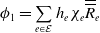 $\phi _1=\sum \limits _{e\in \mathcal{E}}h_e\chi _e{\overline {\overline {R}}}_e$
, then taking
 $\phi =\phi _1-P_h\phi _1, v_h=-P_h\phi _1$
into (3.8) and using (3.23) and (3.2), we have
 \begin{align*} \begin{aligned} \sum _{T\in \mathcal{T}}&\sum _{e\in \partial T}\langle R_e,\phi _1\rangle _e=a_{u}(u-u_h,\phi _1-P_h\phi _1)-\sum _{T\in \mathcal{T}}\Big (R_T,\sum _{e\in {\partial T}}h_e\chi _e{\overline {\overline {R}}}_e\Big )_{T} +J(u_h,P_h\phi _1)\\ &\qquad \qquad \qquad -k^2\varepsilon \big ((\vert u \vert ^2-\left \vert u_h \right \vert ^2\!)u_h,\phi _1-P_h\phi _1\big )_{\Omega _{0}}\\ &= b(u-P_hu,\phi _1-P_h\phi _1)-\big ((k^2+1+k^2\varepsilon {\mathbf{1}}_{\Omega _{0}}\vert u\vert ^2)(u-u_h),\phi _1-P_h\phi _1\big ) +J(u_h,P_h\phi _1)\\ & \quad +\mathbf{i} k\langle u-u_h,\phi _1-P_h\phi _1\rangle _{\Gamma _{\textrm {imp}}}-\sum _{T\in \mathcal{T}}\Big (R_T,\sum _{e\in \partial T}h_e\chi _e{\overline {\overline {R}}}_e\Big )_T-k^2\varepsilon \big ((\vert u\vert ^2-\vert u_h\vert ^2)u_h,\phi _1-P_h\phi _1\big )_{\Omega _{0}} \\ &\lesssim |b(u-P_hu,\phi _1)|+k^2\left \Vert u-u_h\right \Vert _0h^\alpha _{\mathcal{T}}\left \Vert \phi _1\right \Vert _1 +|\gamma |\eta _{\mathcal{T}}\|\phi _1\|_1 + k\Vert u-u_h\Vert _{0,\Gamma _{\textrm {imp}}}h^{\frac \alpha 2}_{\mathcal{T}}\Vert \phi _1\Vert _1 \\ &\quad +\Big (\!\sum _{T\in \mathcal{T}}h_T^2\Vert R_T\Vert ^2_{0,T}\Big )^{\frac 12}\Big (\!\sum _{T\in \mathcal{T}}h_T\Vert {\overline {\overline {R}}}_{\partial T}\Vert ^2_{0,\partial T}\Big )^{\frac 12}+k\left \Vert u-u_h\right \Vert _{0}h^\alpha _{\mathcal{T}}\Vert \phi _1\Vert _1\\ &\lesssim \Big (\Vert u-P_hu\Vert _1+k^2h^\alpha _{\mathcal{T}}\left \Vert u-u_h\right \Vert _{0} +|\gamma |\eta _{\mathcal{T}} +kh^{\frac \alpha 2}_{\mathcal{T}}\Vert u-u_h\Vert _{0,\Gamma _{\textrm {imp}}} \\ &\quad +\Big (\!\sum _{T\in \mathcal{T}}h_T^2\Vert R_T\Vert ^2_{0,T}\Big )^{\frac 12}\Big )\Big (\!\sum _{T\in \mathcal{T}}h_T\Vert {\overline {\overline {R}}}_{\partial T}\Vert ^2_{0,{\partial T}}\Big )^{\frac 12}, \end{aligned} \end{align*}
where we have used
 $\Vert \phi _1\Vert ^2_1\lesssim \sum _{e\in \mathcal{E}}h_e^2\big\Vert \chi _e {\overline {\overline { R}}}_e\big\Vert _{1,\Omega _e}^2 \lesssim \sum _{T\in \mathcal{T}}h_T\Vert {\overline {\overline {R}}}_{\partial T}\Vert ^2_{0,{\partial T}}$
in the last inequality. Then from (3.4) and (3.5), we can deduce that
 \begin{align*} \begin{aligned} \sum \limits _{T\in \mathcal{T}}h_T\left \Vert {\overline {\overline {R}}}_{\partial T}\right \Vert ^2_{0,\partial T}&\eqsim \sum \limits _{T\in \mathcal{T}}\sum \limits _{e\in \partial T}\langle {\overline {\overline { R}}}_e,\phi _1\rangle _e=\sum \limits _{T\in \mathcal{T}}\sum \limits _{e\in \partial T}\big (\langle R_e,\phi _1\rangle _e+\langle {\overline {\overline {R}}}_e-R_e,\phi _1\rangle _e\big )\\ &\lesssim \Big (\| u-P_hu \|_1+\big (t(k,h_{\mathcal{T}}) +|\gamma | \big )\eta _{\mathcal{T}}+\Big (\!\sum _{T\in \mathcal{T}}h_T^2\Vert R_T\Vert ^2_{0,T}\Big )^{\frac 12}\Big )\Big (\!\sum _{T\in \mathcal{T}}h_T\Vert {\overline {\overline {R}}}_{\partial T}\Vert ^2_{0,{\partial T}}\Big )^{\frac 12}\\ &\quad +\Big (\!\sum _{T\in \mathcal{T}}h_T\Vert {\overline {\overline {R}}}_{\partial T}-R_{\partial T}\Vert ^2_{0,{\partial T}}\Big )^{\frac 12}\Big (\!\sum _{T\in \mathcal{T}}h_T\Vert {\overline {\overline {R}}}_{\partial T}\Vert ^2_{0,{\partial T}}\Big )^{\frac 12}. \end{aligned} \end{align*}
By taking the estimate (3.22) into the above inequation, we can derive that
 \begin{align} \sum \limits _{T\in \mathcal{T}}h_T\Vert R_{\partial T}\Vert ^2_{0,{\partial T}}\lesssim \Vert u-P_hu\Vert _1^2+t^2(k,h_{\mathcal{T}})\eta ^2_{\mathcal{T}} +|\gamma |^2\eta ^2_{\mathcal{T}} +\textrm {osc}^2_{\mathcal{T}}. \end{align}
Combining (3.22) and (3.24), we obtain
 $\eta _{\mathcal{T}}^2\lesssim \Vert u-P_hu\Vert ^2_1+t^2(k,h_{\mathcal{T}})\eta _{\mathcal{T}}^2 +|\gamma |^2\eta ^2_{\mathcal{T}} +\textrm {osc}^2_{\mathcal{T}}$
, which implies (3.18) if
 $k^3h^{1+\alpha }_{\mathcal{T}}$
and
 $|\gamma |$
are sufficiently small.
The local lower bound (3.20) can be derived similarly by taking
 $\phi =\varphi _T\overline {\overline {R_T}}, v_h=0$
and
 $\phi =\sum _{e\in \partial T}h_e\chi _e\overline {\overline {R_e}},$
 $v_h=0$
in (3.8), respectively.
On the other hand, from the standard estimate of the a posteriori lower bound (see, e.g., [Reference Morin, Nochetto and Siebert43]), we can obtain
 \begin{align} \widetilde {\eta }_{\mathcal{T}}^2\lesssim \Vert u-P_hu\Vert ^2_1+\widetilde {\textrm {osc}}^2_{\mathcal{T}}. \end{align}
To prove (3.19), it remains to estimate the difference between
 $\textrm {osc}_T$
and
 $\widetilde {\textrm {osc}}_T$
. Similar to (2.29) and (2.30), we have
 $\left \Vert P_hu\right \Vert _{L^{\infty }(\Omega _{0})}\lesssim \left \vert \ln h_{\mathcal{T},\textrm {min}} \right \vert ^{\frac 12} k^{-\frac 12} \widehat {M}(f,g)$
if
 $k^3h_{\mathcal{T}}^2\lesssim 1$
. Therefore,
 \begin{align*} \begin{aligned} \!\!\vert \widetilde {\textrm {osc}}_T&-\textrm {osc}_T\vert ^2\leq h^2_{T}\big \Vert \widetilde R_{T}-R_{T}-\overline {\overline {\widetilde {R}_{T}-R_{T}}}\big \Vert ^2_{0,T}+h_T\big \Vert \widetilde {R}_{\partial T}-R_{\partial T}-\overline {\overline {\widetilde {R}_{\partial T}-R_{\partial T}}}\big \Vert ^2_{0,{\partial T}}\\ &= h^2_{T}\big \Vert \big (k^2(1+\varepsilon {\mathbf{1}}_{\Omega _{0}}\vert u \vert ^2)+1\big )u-\overline {\overline {\big (k^2(1+\varepsilon {\mathbf{1}}_{\Omega _{0}}\vert u \vert ^2)+1\big )u}}\big \Vert _{0,T}+h_T\Vert \mathbf{i} k(u-\overline {\overline {u}})\Vert _{0,\partial T\cap \Gamma _{\textrm {imp}}}\\ &\leq h^2_{T}\big \Vert (k^2+1)(u-P_hu)+k^2\varepsilon {\mathbf{1}}_{\Omega _{0}}\big ((\vert u\vert ^2-\vert P_hu\vert ^2)u+\vert P_hu\vert ^2(u-P_hu)\big )\big \Vert ^2_{0,T}\!+h_T\Vert \mathbf{i} k(u-P_hu)\Vert ^2_{0,{\partial T}\cap \Gamma _{\textrm {imp}}}\\ &\lesssim \big (k^4h^2_T\Vert u-P_hu\Vert _{0,T}^2+k^2h_T\Vert u-P_hu\Vert ^2_{0,{\partial T}\cap \Gamma _{\textrm {imp}}}\big ). \end{aligned} \end{align*}
From the definitions of
 $\textrm {osc}_{\mathcal{T}}$
and
 $\widetilde {\textrm {osc}}_{\mathcal{T}}$
, (3.6),
 $k^3h_{\mathcal{T}}^{1+\alpha }\leq C_0$
and trace inequality, we have
 \begin{align} \begin{aligned} \vert \widetilde {\textrm {osc}}_{\mathcal{T}}-\textrm {osc}_{\mathcal{T}}\vert ^2&\leq \sum \limits _{T\in \mathcal{T}}\vert \widetilde {\textrm {osc}}_T-\textrm {osc}_T\vert ^2\lesssim k^4h_{\mathcal{T}}^2\left \Vert u-P_hu\right \Vert _{0}^2+k^2h_{\mathcal{T}}\left \Vert u-P_hu\right \Vert _{0,\Gamma _{\textrm {imp}}}^2\\ &\lesssim (k^4h_{\mathcal{T}}^2 h_{\mathcal{T}}^{2\alpha }+k^2h_{\mathcal{T}} h_{\mathcal{T}}^{\alpha })\eta _{\mathcal{T}}^2\lesssim \eta _{\mathcal{T}}^2. \end{aligned} \end{align}
Remark 3.7. (i) Combining (3.6) with (3.18), we get
 $\eta _{\mathcal{T}}\eqsim \left \Vert u-P_hu\right \Vert _{1}+\mathrm {osc}_{\mathcal{T}}$
. That is to say, the error estimator of
 $u_h$
fits the error of
 $P_hu$
well and underestimates seriously the error of
 $u_h$
in the preasymptotic regime. This behaviour is first observed by Babuška et al. [
Reference Babuška, Ihlenburg, Strouboulis and Gangaraj3
] for a one-dimensional linear problem. We prove this observation for the first time for the NLH problem.
(ii) From (3.26), there exists a constant
 $C_{\mathrm {osc}}$
such that for any
 $\mathcal{M}\subset \mathcal{T}$
, the following estimate holds
 \begin{align} \vert \mathrm {osc}_{\mathcal{M}}-\widetilde {\mathrm {osc}}_{\mathcal{M}}\vert ^2\leq C_{\mathrm {osc}} (k^4h_{\mathcal{T}}^2 h_{\mathcal{T}}^{2\alpha }+k^2h_{\mathcal{T}} h_{\mathcal{T}}^{\alpha })\eta _{\mathcal{T}}^2. \end{align}
This estimate will be used twice subsequently.
3.3. Equivalent relationships between two error estimators
In this subsection, we establish the equivalence between
 $\eta _{\mathcal{M}}$
and
 $\widetilde {\eta }_{\mathcal{M}}$
in the following sense.
Lemma 3.8.
There exist
 $C_{\mathrm {eq}}$
and
 $\widetilde C_{\mathrm {eq}}$
satisfying
 $C_{\mathrm {eq}}\widetilde C_{\mathrm {eq}}\geq 1$
such that if
 $\left \vert \ln h_{\mathcal{T},\mathrm {min}} \right \vert \varepsilon \widehat {M}(f,g)^2\leq \theta _0$
and
 $\ k^3h_{\mathcal{T}}^{1+\alpha }\leq C_0$
, then the following estimates hold for any
 $\mathcal{M}\subset \mathcal{T}$
:
 \begin{align} \eta _{\mathcal{M}}&\leq C_{\mathrm {eq}}\big (\widetilde {\eta }_{\mathcal{M}}+(t(k,h_{\mathcal{T}})+|\gamma |)\eta _{\mathcal{T}}\big ),\\[-10pt]\nonumber \end{align}
 \begin{align} \widetilde {\eta }_{\mathcal{M}}&\leq \widetilde C_{\mathrm {eq}}\big (\eta _{\mathcal{M}}+(t(k,h_{\mathcal{T}})+|\gamma |)\eta _{\mathcal{T}}\big ). \end{align}
Proof. Similar to (3.8), for any
 $\phi \in H^1_{\Gamma _{\textrm {Dir}}}(\Omega )$
, we have
 \begin{align*} b(u-P_hu,\phi )=\sum \limits _{T\in \mathcal{T}}\big ((\widetilde {R}_T,\phi )_T+\langle \widetilde {R}_{\partial T},\phi \rangle _{\partial T}\big ). \end{align*}
On the other hand, it follows from the definitions of
 $a_u(\cdot ,\cdot )$
,
 $b(\cdot ,\cdot )$
and (2.18):
 \begin{align*} &b(u-P_hu,\phi )=b(u-u_h,\phi -P_h\phi )\\ & \quad =a_{u}(u-u_h,\phi -P_h\phi )+\big ((k^2+1+k^2\varepsilon {\mathbf{1}}_{\Omega _{0}}\vert u \vert ^2)(u-u_h),\phi -P_h\phi \big )-\mathbf{i} k\langle u-u_h,\phi -P_h\phi \rangle _{\Gamma _{\textrm {imp}}}. \end{align*}
By combining (3.8) with the above two identities, we obtain
 \begin{align} &\sum _{T\in \mathcal{T}}\big ((R_T,\phi )_T+\langle R_{\partial T},\phi \rangle _{\partial T}\big )=\sum \limits _{T\in \mathcal{T}}\big ((\widetilde {R}_T,\phi )_T+\langle \widetilde {R}_{\partial T},\phi \rangle _{\partial T}\big )-k^2\varepsilon \big ((\vert u\vert ^2-\vert u_h\vert ^2)u_h,\phi -P_h\phi \big )_{\Omega _{0}}\nonumber\\&\quad +J(u_h,P_h\phi ) -\big ((k^2+1+k^2\varepsilon {\mathbf{1}}_{\Omega _{0}}\vert u\vert ^2)(u-u_h),\phi -P_h\phi \big )+\mathbf{i} k\langle u-u_h,\phi - P_h\phi \rangle _{\Gamma _{\textrm {imp}}}. \end{align}
Denote by
 $\widetilde {\mathcal{M}}\,:\!=\,\bigcup _{T\in \mathcal{M}}\Sigma _{\mathcal{T}}(T)$
. Taking
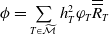 $\phi =\sum \limits _{T\in \widetilde {\mathcal{M}}}h^2_{T}\varphi _{T}{\overline {\overline {R}}}_{T}$
in (3.30), we get
 \begin{align*} \begin{aligned} \sum _{T\in \widetilde {\mathcal{M}}}(R_{T},\phi )_{T}&=\sum _{T\in \widetilde {\mathcal{M}}}(\widetilde R_{T},\phi )_{T}-k^2\varepsilon \big ((\vert u\vert ^2-\vert u_h\vert ^2)u_h,\phi -P_h\phi \big )_{\Omega _{0}} +J(u_h,P_h\phi )\\ &\quad -\big ((k^2+1+k^2\varepsilon {\mathbf{1}}_{\Omega _{0}}\vert u\vert ^2)(u-u_h),\phi -P_h\phi \big )+\mathbf{i} k\langle u-u_h,\phi -P_h\phi \rangle _{\Gamma _{\textrm {imp}}}. \end{aligned} \end{align*}
Then, it follows from (3.21) and (2.19) that
 \begin{align*} \begin{aligned} &\sum _{T\in \widetilde {\mathcal{M}}}h^2_{T}\Vert {\overline {\overline {R}}}_{T}\Vert ^2_{0,T}\lesssim \sum _{T\in \widetilde {\mathcal{M}}}h^2_{T}({\overline {\overline { R}}}_{T},\varphi _{T}{\overline {\overline { R}}}_{T})_{T}=\sum _{T\in \widetilde {\mathcal{M}}}h^2_{T}(R_{T},\varphi _{T}{\overline {\overline { R}}}_{T})_{T}+\sum _{T\in \widetilde {\mathcal{M}}}h^2_{T}({\overline {\overline { R}}}_{T}-R_{T},\varphi _{T}{\overline {\overline {R}}}_{T})_{T}\\ &\quad =\sum _{T\in \widetilde {\mathcal{M}}}h^2_{T}(\widetilde {R}_{T},\varphi _{T}{\overline {\overline { R}}}_{T})_{T}+\sum _{T\in \widetilde {\mathcal{M}}}h^2_{T}({\overline {\overline { R}}}_{T}-R_{T},\varphi _{T}{\overline {\overline {R}}}_{T})_{T} +J(u_h,P_h\phi ) +\mathbf{i} k\langle u-u_h,\phi -P_h\phi \rangle _{\Gamma _{\textrm {imp}}}\\ & \quad -k^2\varepsilon \big ((\vert u\vert ^2-\vert u_h\vert ^2)u_h,\phi -P_h\phi \big )_{\Omega _{0}}-\big ((k^2+1+k^2\varepsilon {\mathbf{1}}_{\Omega _{0}}\vert u\vert ^2)(u-u_h),\phi -P_h\phi \big )\\& \quad \lesssim \sum _{T\in \widetilde {\mathcal{M}}}h^2_{T}\Vert \widetilde {R}_{T}\Vert _{0,T}\Vert {\overline {\overline { R}}}_{T}\Vert _{0,T}+\sum _{T\in \widetilde {\mathcal{M}}}h^2_{T}\Vert R_{T}-{\overline {\overline { R}}}_{T}\Vert _{0,T}\Vert {\overline {\overline {R}}}_{T}\Vert _{0,T} +|\gamma |\eta _{\mathcal{T}}\|\phi \|_1\\ & \quad +k\Vert u-u_h\Vert _{0,\Gamma _{\textrm {imp}}}h^{\frac \alpha 2}_{\mathcal{T}}\Vert \phi \Vert _1+k\left \Vert u-u_h\right \Vert _{0}h_{\mathcal{T}}^{\alpha }\Vert \phi \Vert _1+k^2\Vert u-u_h\Vert _0h_{\mathcal{T}}^{\alpha }\Vert \phi \Vert _1\\& \quad \lesssim \bigg (\Big (\!\sum _{T\in \widetilde {\mathcal{M}}}h^2_{T}\Vert \widetilde {R}_{T}\Vert ^2_{0,T}\Big )^{\frac 12}+\big (t(k,h_{\mathcal{T}}) +|\gamma |\big )\eta _{\mathcal{T}}+\Big (\!\sum _{T\in \widetilde {\mathcal{M}}}h^2_{T}\Vert R_{T}-{\overline {\overline { R}}}_{T}\Vert _{0,T}^2\Big )^{\frac 12}\bigg )\Big (\!\sum _{T\in \widetilde {\mathcal{M}}}h^2_{T}\Vert {\overline {\overline { R}}}_{T}\Vert ^2_{0,T}\Big )^{\frac 12}, \end{aligned} \end{align*}
where we have used
 $\Vert \phi \Vert ^2_1\lesssim \sum _{T\in \widetilde {\mathcal{M}}}h^4_{T}\Vert \varphi _T{\overline {\overline { R}}}_T\Vert ^2_{1,T}\lesssim \sum _{T\in \widetilde {\mathcal{M}}}h^2_{T}\Vert {\overline {\overline {R}}}_T\Vert ^2_{0,T}$
, (3.2), the upper bounds (3.4) and (3.5), and (2.22) to derive the last inequality. Then, we proceed
 \begin{align} \sum _{T\in \widetilde {\mathcal{M}}}h^2_{T}\Vert R_{T}\Vert ^2_{0,T}\lesssim \sum _{T\in \widetilde {\mathcal{M}}}h^2_{T}\Vert \widetilde {R}_{T}\Vert ^2_{0,T}+\big (t^2(k,h_{\mathcal{T}})+|\gamma |^2\big )\eta ^2_{\mathcal{T}}+\sum _{T\in \widetilde {\mathcal{M}}}h^2_{T}\Vert R_{T}-{\overline {\overline {R}}}_{T}\Vert _{0,T}^2. \end{align}
Denote
 $\mathcal{E}_{\mathcal{M}}$
the set of all edges in
 $\mathcal{M}$
and let
 $\phi =\sum _{e\in \mathcal{E}_{\mathcal{M}}}h_e\chi _e {\overline {\overline {R}}}_e$
in (3.30). From (3.23) and (2.19), we have
 \begin{align*} \begin{aligned} \bigg |\sum _{T\in \widetilde {\mathcal{M}}}\sum _{\substack {e\subset \partial T\\e\in \mathcal{E}_{\mathcal{M}}}}\langle R_e,\phi \rangle _e\bigg |&= \bigg |-\sum _{T\in \widetilde {\mathcal{M}}}(R_T,\phi )_T + \sum \limits _{T\in \widetilde {\mathcal{M}}}\big ((\widetilde {R}_T,\phi )_T+\langle \widetilde {R}_{\partial T},\phi \rangle _{\partial T}\big ) +J(u_h,P_h\phi ) +\mathbf{i} k\langle u-u_h,\phi -P_h\phi \rangle _{\Gamma _{\textrm {imp}}}\\ &\quad -k^2\varepsilon \big ((\vert u\vert ^2-\vert u_h\vert ^2)u_h,\phi -P_h\phi \big )_{\Omega _{0}}-\big ((k^2+1+k^2\varepsilon {\mathbf{1}}_{\Omega _{0}}\vert u\vert ^2)(u-u_h),\phi -P_h\phi \big )\bigg |\\ &\lesssim \Big (\!\sum _{T\in \widetilde {\mathcal{M}}}h^2_{T}\Vert R_{T}\Vert ^2_{0,T}+\sum _{T\in \widetilde {\mathcal{M}}}h^2_{T}\Vert \widetilde R_{T}\Vert ^2_{0,T}+\sum _{T\in \mathcal{M}}h_T\Vert \widetilde R_{\partial T}\Vert ^2_{0,{\partial T}}\Big )^{\frac 12}\Big (\!\sum _{T\in \mathcal{M}}h_T\Vert {\overline {\overline {R}}}_{\partial T}\Vert ^2_{0,{\partial T}}\Big )^{\frac 12}\\ &\quad +\big ( |\gamma |\eta _{\mathcal{T}} + kh^{\frac \alpha 2}_{\mathcal{T}}\| u-u_h \|_{0,\Gamma _{\textrm {imp}}}+k^2h^\alpha _{\mathcal{T}}\| u-u_h \|_0\big )\| \phi \|_1. \end{aligned} \end{align*}
We can easily find that
 \begin{equation*}\left \Vert \phi \right \Vert _{1}^2\lesssim \sum _{e\in \mathcal{E}_{\mathcal{M}}}h_e^2\left \Vert \chi _e {\overline {\overline {R}}} _e\right \Vert _{1,\Omega _e}^2\lesssim \sum _{T\in \mathcal{M}} h_T \left \Vert {\overline {\overline {R}}}_{\partial T}\right \Vert _{0,\partial T}^2 ,\end{equation*}
then we deduce from (3.31) that
 \begin{align*} \sum _{T\in \mathcal{M}} h_T \left \Vert {\overline {\overline {R}}}_{\partial T}\right \Vert _{0,\partial T}^2&\eqsim \sum _{T\in \widetilde {\mathcal{M}}}\sum _{\substack {e\subset \partial T\\e\in \mathcal{E}_{\mathcal{M}}}}\langle {\overline {\overline {R}}}_e, h_e\chi _e {\overline {\overline {R}}}_e\rangle _e =\sum _{T\in \widetilde {\mathcal{M}}}\sum _{\substack {e\subset \partial T\\e\in \mathcal{E}_{\mathcal{M}}}}\langle R_e, \phi \rangle _e + \sum _{T\in \widetilde {\mathcal{M}}}\sum _{\substack {e\subset \partial T\\e\in \mathcal{E}_{\mathcal{M}}}}\langle {\overline {\overline {R}}}_e-R_e, \phi \rangle _e \\ &\lesssim \Big (\!\sum _{T\in \widetilde {\mathcal{M}}}h^2_{T}\big (\| \widetilde R_{T} \|_{0,T}^2+\| R_{T}-{\overline {\overline {R}}}_{T} \|^2_{0,T}\big ) + \sum _{T\in \mathcal{M}} h_T\| \widetilde R_{\partial T} \|_{0,\partial T}^2 \\ &\quad +\big (t^2(k,h_{\mathcal{T}})+|\gamma |^2\big )\eta ^2_{\mathcal{T}} + \sum _{T\in \mathcal{M}} h_T\left \Vert R_{\partial T}-{\overline {\overline {R}}}_{\partial T}\right \Vert _{0,\partial T}^2\!\Big )^{\frac 12}\Big (\!\sum _{T\in \mathcal{M}} h_T \left \Vert {\overline {\overline {R}}}_{\partial T}\right \Vert _{0,\partial T}^2\Big )^{\frac 12}. \end{align*}
As a consequence, we have the following estimate with the aid of the triangle inequality
 \begin{align*} \sum _{T\in \mathcal{M}} h_T \left \Vert R_{\partial T}\right \Vert _{0,\partial T}^2&\lesssim \sum _{T\in \widetilde {\mathcal{M}}}h^2_{T}\big (\| \widetilde R_{T} \|_{0,T}^2+\| R_{T}-{\overline {\overline {R}}}_{T} \|^2_{0,T}\big )+ \sum _{T\in \mathcal{M}}h_T\| \widetilde R_{\partial T} \|_{0,\partial T}^2\\ &\quad +\big (t^2(k,h_{\mathcal{T}})+|\gamma |^2\big )\eta ^2_{\mathcal{T}} + \sum _{T\in \mathcal{M}} h_T\left \Vert R_{\partial T}-{\overline {\overline {R}}}_{\partial T}\right \Vert _{0,\partial T}^2. \end{align*}
Altogether with (3.31) and (3.27), it reads
 \begin{align*} \begin{aligned} \eta _{\mathcal{M}}^2&\eqsim \sum _{T\in \widetilde {\mathcal{M}}}h^2_{T}\Vert R_{T}\Vert ^2_{0,T}+\sum _{T\in \mathcal{M}} h_T \left \Vert R_{\partial T}\right \Vert _{0,\partial T}^2\\ &\lesssim \widetilde {\eta }_{\mathcal{M}}^2+\big (t^2(k,h_{\mathcal{T}})+|\gamma |^2\big )\eta _{\mathcal{T}}^2+ \sum _{T\in \widetilde {\mathcal{M}}}h^2_{T}\| R_{T}-{\overline {\overline {R}}}_{T} \|^2_{0,T}+\sum _{T\in \mathcal{M}} h_T\left \Vert R_{\partial T}-{\overline {\overline {R}}}_{\partial T}\right \Vert _{0,\partial T}^2\\ &\lesssim \widetilde {\eta }_{\mathcal{M}}^2+\big (t^2(k,h_{\mathcal{T}})+|\gamma |^2\big )\eta _{\mathcal{T}}^2+\widetilde \eta _{\mathcal{M}}^2+(k^4h_{\mathcal{T}}^{2+2\alpha }+k^2h_{\mathcal{T}}^{1+\alpha })\eta _{\mathcal{T}}^2\\ &\lesssim \widetilde {\eta }_{\mathcal{M}}^2+\big (t^2(k,h_{\mathcal{T}})+|\gamma |^2\big )\eta _{\mathcal{T}}^2. \end{aligned} \end{align*}
By the similar argument, we arrive at
 \begin{align*} \widetilde \eta _{\mathcal{M}}^2&\lesssim \eta _{\mathcal{M}}^2 +\big (t^2(k,h_{\mathcal{T}})+|\gamma |^2\big )\eta _{\mathcal{T}}^2+\sum _{T\in \widetilde {\mathcal{M}}}h^2_{T}\| \widetilde R_{T}-\overline {\overline {\widetilde R_{T}}} \|^2_{0,T}+\sum _{T\in \mathcal{M}} h_T\left \Vert \widetilde R_{\partial T}-\overline {\overline {\widetilde R_{\partial T}}}\right \Vert _{0,\partial T}^2\\ &\lesssim \eta _{\mathcal{M}}^2 +\big (t^2(k,h_{\mathcal{T}})+|\gamma |^2\big )\eta _{\mathcal{T}}^2. \end{align*}
It is natural to derive the following two corollaries. The first one is the equivalence on the whole mesh and the second one is an equivalence between the so-called Dörfler marking strategies for
 $u_h$
and
 $P_hu$
.
Corollary 3.9.
Under the assumptions of Lemma 3.8
, if in addition
 $(t(k,h_{\mathcal{T}})+|\gamma |)\leq \frac {1}{2C_{\mathrm {eq}}}$
, then
 $\eta _{\mathcal{T}}\eqsim \widetilde {\eta }_{\mathcal{T}}$
.
Corollary 3.10.
Under the assumptions of Lemma 3.8
, it holds for
 $\theta _{D}\in (0,1], \eta _{\mathcal{M}}\geq \theta _D\eta _{\mathcal{T}}$
, and
 $(t(k,h_{\mathcal{T}})+|\gamma |)\leq \frac {\theta _D}{C_{\mathrm {eq}}}$
,
 \begin{align*} \widetilde \eta _{\mathcal{M}}\geq \widetilde \theta _D\widetilde \eta _{\mathcal{T}}\quad \text{with} \quad \widetilde {\theta }_D=\frac {\theta _D-C_{\mathrm {eq}}(t(k,h_{\mathcal{T}})+|\gamma |)}{C_{\mathrm {eq}} \widetilde C_{\mathrm {eq}}(1+t(k,h_{\mathcal{T}})+|\gamma |)}. \end{align*}
Proof. It follows form (3.28)-(3.29) that
 \begin{align*} \widetilde \eta _{\mathcal{M}}\ge &\ \frac {\eta _{\mathcal{M}}}{C_{\textrm {eq}}}-(t(k,h_{\mathcal{T}})+|\gamma |)\eta _{\mathcal{T}} \ge \ \frac {\theta _D\eta _{\mathcal{T}}}{C_{\textrm {eq}}}-(t(k,h_{\mathcal{T}})+|\gamma |)\eta _{\mathcal{T}}=\ \widetilde {\theta }_D\widetilde C_{\textrm {eq}}(1+t(k,h_{\mathcal{T}})+|\gamma |)\eta _{\mathcal{T}}\ge \ \widetilde {\theta }_D\widetilde \eta _{\mathcal{T}}. \end{align*}
4. Convergence and quasi-optimality of the AFEM and ACIPFEM
4.1. Adaptive algorithm
We use
 $n(n \ge 0)$
to represent the iteration number in the adaptive algorithm. In the
 $n$
-th loop, we first solve the CIPFEM (2.14) on
 $\mathcal{T}_n$
, and then calculate the error estimators
 $\eta _T$
for each element
 $T\in \mathcal{T}_n$
. After computing the error estimators, we mark the ‘bad’ mesh
 $\mathcal{M}_n$
by using the Dörfler strategy. Finally, we refine the mesh
 $\mathcal{M}_n$
by the newest vertex bisection algorithm (see, e.g., [Reference Cascon, Kreuzer, Nochetto and Siebert13, Reference Karkulik, Pavlicek and Praetorius35]) at least
 $b\geq 1$
times and remove the hanging nodes and then set
 $n\,:\!=\,n+1$
to the first step. We set
 $V_{n}\,:\!=\,V_{\mathcal{T}_n}$
,
 $h_n\,:\!=\,h_{\mathcal{T}_n}$
,
 $h_{n,\textrm {min}}\,:\!=\,h_{\mathcal{T}_n,\textrm {min}}$
for simplicity.
The basic loop of this adaptive algorithm is given below:
Given the initial triangulation
 $\mathcal{T}_0$
and marking parameter
 $\theta _D \in (0,1],$
set
 $n\,:\!=\,0$
and iterate,
-
1. Solve equation (2.14) on
 $\mathcal{T}_n$
to obtain
$u_n,$
-
2. Calculate the error estimator
$\eta _T(u_n)$
on every element
$T\in \mathcal{T}_{n},$
-
3. Mark
$\mathcal{M}_n \subset \mathcal{T}_n$
with minimal cardinality such that
$ \eta _{\mathcal{M}_n} \ge \theta _D \eta _{\mathcal{T}_n},$
-
4. Refine
$\mathcal{M}_n$
using the newest vertex bisection algorithm to get
$\mathcal{T}_{n+1}$
, -
5. Set
$n\,:\!=\,n+1$
and then go to step 1.


Remark 4.1.
(i) Unlike the algorithm in [
Reference Duan and Wu21
] which refines the broader mesh
 $\widetilde {\mathcal{M}}_n\,:\!=\,\bigcup _{T\in \mathcal{M}_n}\Sigma _{\mathcal{T}_n}(T)$
in order to apply the equivalent relationships of the error estimators to derive the convergence and quasi-optimality of
 $u_n$
, the above adaptive algorithm is the same as the standard adaptive algorithm for elliptic problems since we modify the definitions of error estimators.
(ii) In step 1, we assume solving (2.14) is accurate but in practical computation we utilize Newton’s iteration until the relative error between two consecutive iterative solutions falls below a prescribed tolerance. Indeed, when using the frozen-nonlinearity iteration with the iteration number fixed, it is named an adaptive Kačanov method for quasi-linear elliptic partial differential equations (see, e.g., [ Reference Garau, Morin and Zuppa22 ]). For our NLH problem, the convergence cannot be theoretically guaranteed. However, the numerical results are promising with an iteration number specified. We will study this convergence in our future work.
In the next two subsections, we shall prove the convergence and quasi-optimality of the AFEM and ACIPFEM by following the “elliptic projection argument” developed in [Reference Duan and Wu21] for AFEM for the linear Helmholtz equation, that is, after establishing the equivalent relationships in Section 3.3 between the error estimators for the FE solutions and those for the elliptic projections, we transform the analysis of the sequence of CIPFE solutions
 $u_n$
obtained by the ACIPFEM to the analysis of that of the corresponding elliptic projections, denoted by
 $\widetilde u_{n}$
of the exact solution
 $u$
onto
 $V_{n}$
, which can be done by using the well-developed theory of AFEM for elliptic problems (see, e.g., [Reference Cascon, Kreuzer, Nochetto and Siebert13]).
4.2. Convergence of the AFEM and ACIPFEM
In this subsection, we prove the convergence of the AFEM and ACIPFEM by proving the convergence of the sequence of the elliptic projections
 $\widetilde u_{n}$
. But the error estimators
 $\widetilde \eta _{\mathcal{T}}$
for the elliptic projections do not satisfy the so-called “estimator reduction property” (see, e.g., [Reference Cascon, Kreuzer, Nochetto and Siebert13, Corollary 3.4]), which is crucial in the analysis of AFEM for elliptic problems. To overcome this difficulty, we introduce an equivalent auxiliary error estimator for the elliptic projection by tuning the weights before the terms of element residuals:
 \begin{align} \big(\widetilde \eta _T^*\big)^2=h_T^2\big \Vert \widetilde R_T\big \Vert _{0,T}^2+h_T\big \Vert \widetilde R_{{\partial T}}\big \Vert _{0,{\partial T}}^2+\frac {1}{6}h_T^2\sum _{T'\in \Sigma _{\mathcal{T}}(T)\setminus \{T\}}\big \Vert \widetilde R_{T'}\big \Vert _{0,T'}^2. \end{align}
It is clear that there exist positive constants
 $c_1$
and
 $c_2$
such that
 \begin{align*} c_1\widetilde \eta _T \leq \widetilde \eta ^*_T \leq c_2\widetilde \eta _T. \end{align*}
The first lemma gives the distance between the error estimators of two different discrete functions.
Lemma 4.2 (local perturbation). For all
 $T\in \mathcal{T}, v_{h1},v_{h2}\in V_{\mathcal{T}}$
, there exists a positive constant
 $C_{\mathrm {per}}$
, which depends only on the shape regularity of
 $\mathcal{T}_0$
, such that
 \begin{align*} \big \vert \widetilde \eta ^*_T(v_{h1})-\widetilde \eta ^*_T(v_{h2})\big \vert \leq C_{\mathrm {per}}\left \Vert v_{h1}-v_{h2}\right \Vert _{1,\Omega _{\mathcal{T}}(T)}. \end{align*}
Proof. It is from the definitions of
 $\widetilde \eta _T^*$
, the triangle inequality, the trace inequality and the inverse estimate that
 \begin{align*} \big \vert \widetilde \eta _T^*(v_{h1})-\widetilde \eta _T^*(v_{h2})\big \vert ^2&\leq h_{T}^2\left \Vert \widetilde R_T(v_{h1})-\widetilde R_T(v_{h2})\right \Vert _{0,T}^2+h_{T}\left \Vert \widetilde R_{{\partial T}}(v_{h1})-\widetilde R_{{\partial T}}(v_{h2})\right \Vert _{0,{\partial T}}^2\\ &\quad +\frac 1{6}h^2_T\sum _{T'\in \Sigma _{\mathcal{T}}(T)\setminus \{T\}}\left \Vert \widetilde R_{T'}(v_{h1})-\widetilde R_{T'}(v_{h2})\right \Vert _{0,T'}^2 \\ &=h_{T}^2\left \Vert v_{h1}-v_{h2}\right \Vert _{0,T}^2+\frac {h_T}{4}\left \Vert [\![\nabla (v_{h1}-v_{h2})]\!]\right \Vert _{0,{\partial T}\cap \Omega }^2+h_{T}\left \Vert \nabla (v_{h1}-v_{h2})\cdot n\right \Vert _{0,{\partial T}\cap \Gamma _{\textrm {imp}}}^2\\ &\quad +\frac 1{6}h^2_T\sum _{T'\in \Sigma _{\mathcal{T}}(T)\setminus \{T\}}\left \Vert v_{h1}-v_{h2}\right \Vert _{0,T'}^2\\ &\leq C_{\textrm {per}}^2\big (h^2_T\left \Vert v_{h1}-v_{h2}\right \Vert _{0,\Omega _{\mathcal{T}}(T)}^2+\left \Vert \nabla (v_{h1}-v_{h2})\right \Vert _{0,\Omega _{\mathcal{T}}(T)}^2\!\big )\\ &\leq C_{\textrm {per}}^2\left \Vert v_{h1}-v_{h2}\right \Vert _{1,\Omega _{\mathcal{T}}(T)}^2. \end{align*}
Then, the conclusion comes from finding the square root.
The next lemma is the estimator reduction property for the elliptic projection.
Lemma 4.3 (estimator reduction). For every
 $\delta \gt 0$
and
 $b\gt 0$
, letting
 $\lambda _b\,:\!=\,\max \{3\cdot 2^{-(b+1)},2^{-\frac b2}\}$
, there holds
 \begin{align} \widetilde \eta _{\mathcal{T}_{n+1}}^*(\widetilde u_{n+1})^2\leq (1+\delta )\big (\widetilde \eta ^*_{\mathcal{T}_n}(\widetilde u_n)^2-(1-\lambda _b)\widetilde \eta _{\mathcal{M}_n}^*(\widetilde u_n)^2\big )+4(1+\delta ^{-1})C_{\mathrm { per}}^2\left \Vert \widetilde u_n-\widetilde u_{n+1}\right \Vert _{1}^2. \end{align}
Proof. First, it can be directly derived from Lemma 4.2 and the Young’s inequality that
 \begin{align} \widetilde \eta _{\mathcal{T}_{n+1}}^*(\widetilde u_{n+1})^2\leq (1+\delta )\widetilde \eta _{\mathcal{T}_{n+1}}^*(\widetilde u_n)^2+ 4(1+\delta ^{-1})C_{\textrm {per}}^2\left \Vert \widetilde u_{n+1}-\widetilde u_n\right \Vert _{1}^2. \end{align}
Then for
 $T\in \mathcal{T}_n,$
we define
 $T_*\,:\!=\,\{T_1\in \mathcal{T}_{n+1}:\; T_1\subset T\}$
and handle
 $\widetilde \eta _{\mathcal{T}_{n+1}}^*(\widetilde u_{n})^2$
in two parts:
 \begin{align*} \widetilde \eta _{\mathcal{T}_{n+1}}^*(\widetilde u_{n})^2&=\sum _{\substack {T\in \mathcal{M}_n\\ T_1\in T_*}}\widetilde \eta _{T_1}^*(\widetilde u_{n})^2+\sum _{\substack {T\in \mathcal{T}_{n}\setminus \mathcal{M}_n\\ T_1\in T_*}}\widetilde \eta _{T_1}^*(\widetilde u_{n})^2. \end{align*}
Part I: for
 $T\in \mathcal{M}_n$
, we have
 \begin{align*} \sum _{T_1\in T_*}\widetilde \eta _{T_1}^*(\widetilde u_{n})^2&=\sum _{T_1\in T_*}\Bigg (h_{T_1}^2\big \Vert \widetilde R_{T_1}\big \Vert _{0,T_1}^2+h_{T_1}\big \Vert \widetilde R_{\partial T_1}\big \Vert _{0,\partial T_1}^2+\frac 1{6}h^2_{T_1}\sum _{T'\in \Sigma _{\mathcal{T}_{n+1}}(T_1)\setminus \{T_1\}}\big \Vert \widetilde R_{T'}\big \Vert _{0,T'}^2\Bigg )\\ &\leq\sum _{T_1\in T_*}\Bigg (2^{-b}h^2_{T}\big \Vert \widetilde R_{T_1}\big \Vert _{0,T_1}^2+2^{-\frac b2}h_{T}\big \Vert \widetilde R_{\partial T_1}\big \Vert _{0,\partial T_1}^2+\frac {2^{-b}}{6}h_T^2\sum _{\substack {T'\in \Sigma _{\mathcal{T}_{n+1}}(T_1)\setminus \{T_1\}\\ T'\not \subset T}}\big \Vert \widetilde R_{T'}\big \Vert _{0,T'}^2\\ &\quad +\frac {2^{-b}}{6}h_T^2\sum _{\substack {T'\in \Sigma _{\mathcal{T}_{n+1}}(T_1)\setminus \{T_1\}\\ T'\subset T}}\big \Vert \widetilde R_{T'}\big \Vert _{0,T'}^2\Bigg )\\ &\leq 2^{-b}h^2_{T}\big \Vert \widetilde R_T\big \Vert _{0,T}^2+2^{-\frac b2}h_{T}\big \Vert \widetilde R_{{\partial T}}\big \Vert _{0,\partial T}^2+\frac {2^{-b}}{6}h^2_T\sum _{T'\in \Sigma _{\mathcal{T}_n}(T)\setminus \{T\}}\big \Vert \widetilde R_{T'}\big \Vert _{0,T'}^2 +\frac {2^{-b}\cdot 3}{6}h^2_T\big \Vert \widetilde R_T\big \Vert _{0,T}^2\\ &\leq \lambda _b\widetilde \eta ^*_T(\widetilde u_n)^2. \end{align*}
Since
 $\widetilde \eta ^*_{\mathcal{M}_n}(\widetilde u_n)^2=\sum _{T\in \mathcal{M}_n}\widetilde \eta ^*_T(\widetilde u_n)^2$
, we get
 \begin{align} \sum _{\substack {T\in \mathcal{M}_n\\ T_1\in T_*}}\widetilde \eta _{T_1}^*(\widetilde u_{n})^2\leq \lambda _b\widetilde \eta ^*_{\mathcal{M}_n}(\widetilde u_n)^2. \end{align}
Part II: let
 $\mathcal R$
be the set of refined elements in
 $\mathcal{T}_n$
. Exactly,
 $\mathcal{M}_n\subset \mathcal R$
. For
 $T\in \mathcal{T}_n{\setminus}\mathcal R$
,
 $T_*$
equals
 $\{T\}$
, and
 \begin{align*} \sum _{T_1\in T_*}\widetilde \eta _{T_1}^*(\widetilde u_n)^2\leq \widetilde \eta _{T}^*(\widetilde u_n)^2. \end{align*}
On the other hand, for
 $T\in (\mathcal{T}_n{\setminus}\mathcal{M}_n)\cap \mathcal R$
, similar to the first estimate in Part I, we derive
 \begin{align*} \sum _{T_1\in T_*}\widetilde \eta _{T_1}^*(\widetilde u_n)^2&=\sum _{ T_1\in T_*}\Bigg (h_{T_1}^2\big \Vert \widetilde R_{T_1}\big \Vert _{0,T_1}^2+h_{T_1}\big \Vert \widetilde R_{\partial T_1}\big \Vert _{0,\partial T_1}^2+\frac 1{6}h^2_{T_1}\sum _{T'\in \Sigma _{\mathcal{T}_{n+1}}(T_1)\setminus \{T_1\}}\big \Vert \widetilde R_{T'}\big \Vert _{0,T'}^2\Bigg )\leq \lambda _1\widetilde \eta _{T}^*(\widetilde u_n)^2. \end{align*}
As a conclusion, we can get
 \begin{align} \sum _{\substack {T\in \mathcal{T}_{n}\setminus \mathcal{M}_n\\ T_1\in T_*}}\widetilde \eta _{T_1}^*(\widetilde u_{n})^2\leq \sum _{T\in \mathcal{T}_{n}\setminus \mathcal{M}_n}\widetilde \eta _{T}^*(\widetilde u_{n})^2 = \widetilde \eta _{\mathcal{T}_n}^*(\widetilde u_n)^2-\widetilde \eta _{\mathcal{M}_n}^*(\widetilde u_n)^2. \end{align}
Then combining (4.4) and (4.5), we have
 \begin{align} \widetilde \eta _{\mathcal{T}_{n+1}}^*(\widetilde u_{n})^2\leq \widetilde \eta _{\mathcal{T}_n}^*(\widetilde u_n)^2-(1-\lambda _b)\widetilde \eta _{\mathcal{M}_n}^*(\widetilde u_n)^2. \end{align}
Finally, (4.2) comes from (4.3) and (4.6). This completes the proof of the lemma.
The last theorem in this subsection is showing the convergence of the A(CIP)FEM in the case of low energy.
Theorem 4.4 (convergence). Let
 $\theta _D\in (0,1]$
. There exists a constant
 $C_{\mathrm {conv}} \in (0, 1)$
depending only on
 $\mathcal{T}_{0}, b$
and
 $\theta _D$
such that if
 $|\gamma |\leq \gamma _0$
,
 $\vert \ln h_{n,\mathrm {min}}\vert \varepsilon \widehat {M}(f,g)^2\leq \theta _0 \ \text{and} \ k^3h^{1+\alpha }_0\le C_0$
, then
 \begin{align*} \left\Vert {\hskip -4.1pt}\left\vert u-u_n \right\vert {\hskip -4.1pt}\right\Vert \lesssim C_{\mathrm {conv}}^n(1+k^2h_n)\big (kh_0+k^{-\frac 12}(kh_0)^{\alpha }\big ) \widehat {M}(f,g). \end{align*}
Proof. The key point is to prove the contraction property: there exist constants
 $\beta \gt 0$
and
 $C_{\textrm {conv}}\in (0,1)$
such that
 \begin{align} \left \Vert u-\widetilde u_{n+1}\right \Vert _{1}^2+\beta \widetilde \eta _{\mathcal{T}_{n+1}}^*(\widetilde u_{n+1})^2 \leq C_{\textrm {conv}}^2\big (\!\left \Vert u-\widetilde u_n\right \Vert _{1}^2+\beta \widetilde \eta _{\mathcal{T}_n}^*(\widetilde u_n)^2\big ). \end{align}
Combining (2.18) and Lemma 4.3, we choose
 $\beta =\frac 1{4(1+\delta ^{-1})C_{\textrm {per}}^2}$
to get
 \begin{align*} \left \Vert u-\widetilde u_{n+1}\right \Vert _{1}^2+\beta \widetilde \eta _{\mathcal{T}_{n+1}}^*(\widetilde u_{n+1})^2&\leq \left \Vert u-\widetilde u_n\right \Vert _{1}^2-\left \Vert \widetilde u_{n+1}-\widetilde u_n\right \Vert _{1}^2+\beta (1+\delta )\big (\widetilde \eta _{\mathcal{T}_{n}}^*(\widetilde u_{n})^2-(1-\lambda _b) \widetilde \eta _{\mathcal{M}_{n}}^*(\widetilde u_{n})^2\big )\\ &\quad +4\beta (1+\delta ^{-1})C_{\textrm {per}}^2\left \Vert \widetilde u_{n+1}-\widetilde u_n\right \Vert _{1}^2\\ &=\left \Vert u-\widetilde u_n\right \Vert _{1}^2+\beta (1+\delta )\big (\widetilde \eta _{\mathcal{T}_{n}}^*(\widetilde u_{n})^2-(1-\lambda _b) \widetilde \eta _{\mathcal{M}_{n}}^*(\widetilde u_{n})^2\big ). \end{align*}
Noting that
 $\widetilde \eta _{\mathcal{M}_{n}}(\widetilde u_{n})\geq \widetilde \theta _{\textrm {D}} \widetilde \eta _{\mathcal{T}_n}(\widetilde u_n)$
(see Corollary 3.10) and
 $\left \Vert u-\widetilde u_n\right \Vert _{1}\leq C_{\textrm {up}}\widetilde \eta _{\mathcal{T}_n}$
for some constant
 $C_{\textrm {up}}\gt 0$
(see (3.6)) when
 $k^3h^{1+\alpha }$
and
 $|\gamma |$
are sufficiently small, we have
 \begin{align*} \widetilde \eta ^*_{\mathcal{M}_n}\geq c_1\widetilde \eta _{\mathcal{M}_n}\geq c_1\widetilde \theta _{\textrm {D}}\widetilde \eta _{\mathcal{T}_n}\geq \frac {c_1\widetilde \theta _{\textrm {D}}}{c_2}\widetilde \eta ^*_{\mathcal{T}_n},\quad \left \Vert u-\widetilde u_n\right \Vert _{1}\leq \frac {C_{\textrm {up}}}{c_1}\widetilde \eta _{\mathcal{T}_n}^*. \end{align*}
Then, for any
 $\mu \in (0,1)$
,
 \begin{align*} \left \Vert u-\widetilde u_{n+1}\right \Vert _{1}^2+\beta \big(\widetilde \eta _{\mathcal{T}_{n+1}}^*\big)^2&\leq \Big (1-\beta (1+\delta )(1-\lambda _b)\mu \Big (\frac {c_1\widetilde \theta _{\textrm {D}}}{c_2C_{\textrm {up}}}\Big )^2\Big )\left \Vert u-\widetilde u_n\right \Vert _{1}^2\\ &\quad +\beta (1+\delta )\Big (1-(1-\lambda _b)(1-\mu )\Big (\frac {c_1\widetilde \theta _{\textrm {D}}}{c_2}\Big )^2\Big )(\widetilde \eta _{\mathcal{T}_{n}}^*)^2. \end{align*}
To obtain (4.7), we let
 \begin{align*} C_{\textrm {conv}}^2=\max \Big \{1-\beta (1+\delta )(1-\lambda _b)\mu \Big (\frac {c_1\widetilde \theta _{\textrm {D}}}{c_2C_{\textrm {up}}}\Big )^2, \,(1+\delta )\Big (1-(1-\lambda _b)(1-\mu )\Big (\frac {c_1\widetilde \theta _{\textrm {D}}}{c_2}\Big )^2\Big )\Big \} \end{align*}
and choose
 $\delta$
sufficiently small such that
 $C_{\textrm {conv}}\lt 1$
.
Finally, it follows from the upper bounds (3.3) and (3.4), the equivalences of and
 $\widetilde \eta _{\mathcal{T}}^*$
, (4.7), and the lower bound (3.19) that
 \begin{align*} \left\Vert {\hskip -4.1pt}\left\vert u-u_n \right\vert {\hskip -4.1pt}\right\Vert &\lesssim (1+k^{\frac 12}(kh_n)^{\alpha }+k^2h_n) \eta _{\mathcal{T}_n}\lesssim (1+k^2h_n) \widetilde \eta _{\mathcal{T}_n}^*\\ &\lesssim (1+k^2h_n)(\!\left \Vert u-\widetilde u_{n}\right \Vert _{1}^2+ \beta (\widetilde \eta _{\mathcal{T}_n}^*)^2)^{1/2}\\ &\lesssim (1+k^2h_n)(\!\left \Vert u-\widetilde u_{0}\right \Vert _{1}+ \widetilde \eta _{\mathcal{T}_0}^*)C_{\textrm {conv}}^n\\ &\lesssim (1+k^2h_n) (\!\left \Vert u-\widetilde u_{0}\right \Vert _{1}+ \textrm {osc}_{\mathcal{T}_0})C_{\textrm {conv}}^n. \end{align*}
Altogether with
 \begin{align} &\textrm {osc}_{\mathcal{T}_0} = {\Big (\!\sum _{T\in \mathcal{T}_0} \big (h_T^2\| f-\overline {\overline {f}} \|^2_{0,T}+ h_T\| g-\overline {\overline {g}} \|_{0,\partial T\cap \Gamma _{\textrm {imp}}}^2\big )\Big )}^{\frac {1}{2}}\lesssim h_0 \big (\| f \|_0+\| g \|_{\frac 12, \Gamma _{\textrm {imp}}}\big ),\\ &{\left \Vert u-\widetilde u_0\right \Vert }_{1}\lesssim (kh_0+k^{-\frac 12}(kh_0)^{\alpha })\widehat {M}(f,g),\notag \end{align}
we get the desired convergence result.
4.3. Quasi-optimality of the AFEM and ACIPFEM
This subsection concerns the quasi-optimality of the AFEM and ACIPFEM. Again we consider the quasi-optimality of
 $\{\widetilde u_n\}_{n\geq 0}$
instead, which can be proved by following the analysis of the AFEM for elliptic problems (see, e.g., [Reference Cascon, Kreuzer, Nochetto and Siebert13, Section 5]), but with a key difference that we have to use the error estimators
 $\eta _T(u_h)$
(instead of
 $\widetilde \eta _T(\widetilde u_h)$
as usual) to characterize the localized upper bound and the optimal marking property associated with the elliptic projections (see Lemmas 4.6 and 4.9 below). Of course, unlike the analysis for the linear Helmholtz equation [Reference Duan and Wu21], we have to deal with the effects of the nonlinear term, where the upper bounds (3.4)–(3.5) will play an important role. The contraction property (4.7) based on our newly introduced auxiliary error estimator in (4.1) is also essential in our proof of the quasi-optimality. We will only give a sketch of the proof by mainly showing the major differences from those in [Reference Cascon, Kreuzer, Nochetto and Siebert13] or [Reference Duan and Wu21].
The first lemma below says that total error
 $(\!\left \Vert u-\widetilde u_n\right \Vert _{1}^2+\widetilde {\textrm {osc}}_{\mathcal{T}_n}^2(\widetilde u_n))^{\frac 12}$
(see [Reference Cascon, Kreuzer, Nochetto and Siebert13, Reference Mekchay and Nochetto39]) of the elliptic projection
 $\widetilde u_n\in V_n$
of
 $u$
satisfies the Cea’s lemma.
Lemma 4.5 (optimality of the total error of
 $\widetilde u_h$
). The following estimate holds
 \begin{align} \left \Vert u-\widetilde u_n\right \Vert _{1}^2+\widetilde {\mathrm {osc}}_{\mathcal{T}_n}^2(\widetilde u_n)\leq \inf _{v_h\in V_{n}}\big (\!\left \Vert u-v_h\right \Vert _{1}^2+\widetilde {\mathrm {osc}}_{\mathcal{T}_n}^2(v_h)\big ). \end{align}
Proof. By the orthogonality of
 $\widetilde u_n$
, we have for any
 $v_h\in V_{n}$
,
 \begin{align*} \left \Vert u-\widetilde u_n\right \Vert _{1}^2=\left \Vert u-v_h\right \Vert _{1}^2-\left \Vert \widetilde u_n-v_h\right \Vert _{1}^2\leq \left \Vert u-v_h\right \Vert _{1}^2. \end{align*}
Moreover, we see from the definition of
 $\widetilde {\textrm {osc}}$
that
 $\widetilde {\textrm {osc}}_{\mathcal{T}_n}(v_h)$
is independent of
 $v_h\in V_{n}$
, and hence (4.9) is derived.
Lemma 4.6 (localized upper bound). Let
 $\mathcal{T}_*$
be a refinement of
 $\mathcal{T}$
and
 $\mathcal R$
be the set of refined elements. Let
 $\widetilde u_{\mathcal{T}_*}$
and
 $\widetilde u_{\mathcal{T}}$
be the corresponding elliptic projections of
 $u$
in
 $V_{\mathcal{T}_*}$
and
 $V_{\mathcal{T}}$
, respectively. Then, there exists a constant
 $C_{\mathrm {lub}}$
such that if
 $\vert \ln h_{\mathcal{T},\mathrm {min}}\vert \varepsilon \widehat {M}(f,g)^2\leq \theta _0 \ \text{and} \ k^3h_{\mathcal{T}}^{1+\alpha }\le C_0$
, then
 \begin{align*} \left \Vert \widetilde u_{\mathcal{T}_*}-\widetilde u_{\mathcal{T}}\right \Vert _{1}^2\leq C_{\mathrm {lub}}\big (\eta _{\mathcal R}^2(u_h)+(t^2(k,h_{\mathcal{T}})+|\gamma |^2)\eta _{\mathcal{T}}^2(u_h)\big ). \end{align*}
Proof. Let
 $\Omega _{\mathcal R}=\cup \{T\,:\,T\in \mathcal R\}$
be the union of refined elements, and denote by
 $\Omega _i, i=1,\ldots ,I$
, the connected components of its interior. We denote
 $\mathcal{T}^i=\{T\in \mathcal{T}\,:\, T\subset \bar \Omega _i\}$
and
 $V_{\mathcal{T}^i}$
be the restriction of
 $V_{\mathcal{T}}$
to
 $\Omega _i$
. For the error
 $E_*\,:\!=\,\widetilde u_{\mathcal{T}_*}-\widetilde u_{\mathcal{T}}$
, we construct
 $\Pi _hE_*\in V_{\mathcal{T}}$
by
 \begin{align*} \Pi _hE_*\,:\!=\,\Pi _{hi} E_*\quad \text{in} \ \Omega _i; \quad \Pi _hE_*\,:\!=\,E_* \quad \text{elsewhere} . \end{align*}
where
 $\Pi _{hi}\,:\, H^1(\Omega _i)\rightarrow V_{\mathcal{T}^i}$
is the standard Scott–Zhang interpolation operator satisfying
 $\Pi _{hi} E_*=E_*$
on each
 $\partial \Omega _i$
(see, e.g. [Reference Scott and Zhang44]). Indeed, since
 $E_*$
has conforming boundary values on
 $\partial \Omega _i$
in
 $V_{\mathcal{T}^i}$
, we have
 $\Pi _hE_*\in V_{\mathcal{T}}$
.
We denote
 $\psi _1=E_*-\Pi _hE_*$
. By the orthogonality and error estimate of the elliptic projection, (3.8) with
 $\phi =\psi _1-P_h\psi _1$
and
 $v_h=-P_h\psi _1\in V_{\mathcal{T}}$
, (3.2) and upper bounds (3.4)–(3.5), we derive
 \begin{align*} b(E_*,E_*)&=b(E_*,E_*-\Pi _hE_*)=b(u-\widetilde u_{\mathcal{T}},\psi _1)\\ &=b(u-\widetilde u_{\mathcal{T}},\psi _1-P_h\psi _1)=b(u-u_h,\psi _1-P_h\psi _1)\\ &=a_u(u-u_h,\psi _1-P_h\psi _1)+\big ((k^2+1+k^2\varepsilon {\mathbf{1}}_{\Omega _{0}}\vert u \vert ^2)(u-u_h),\psi _1-P_h\psi _1\big )\\ &\quad -\mathrm ik\left \langle {u-u_h},{\psi _1-P_h\psi _1}\right \rangle _{\Gamma _{\textrm {imp}}} \\ &\lesssim \eta _{\mathcal R}(u_h)\left \Vert \nabla \psi _1\right \Vert _{0} +|\gamma |\eta _{\mathcal{T}}\left \Vert \nabla \psi _1\right \Vert _{0} +k^2\varepsilon \big\vert \big ((\vert u \vert ^2-\left \vert u_h \right \vert ^2\!)u_h,\psi _1-P_h\psi _1\big )_{\Omega _{0}} \big\vert \\ &\quad +k^2\left \Vert u-u_h\right \Vert _{0}h_{\mathcal{T}}^{\alpha }\left \Vert \psi _1\right \Vert _{1}+kh^{\frac {\alpha }2}_{\mathcal{T}}\left \Vert u-u_h\right \Vert _{0,\Gamma _{\textrm {imp}}}\left \Vert \psi _1\right \Vert _{1}\\ &\lesssim \eta _{\mathcal R}(u_h)\left \Vert E_*\right \Vert _{1,\Omega _{\mathcal R}}+(t(k,h_{\mathcal{T}})+|\gamma |)\eta _{\mathcal{T}}\left \Vert E_*\right \Vert _{1,\Omega _{\mathcal R}}\!. \end{align*}
This completes the proof of the lemma.
Recalling [Reference Cascon, Kreuzer, Nochetto and Siebert13, Lemma 2.3], we can directly get the following Lemma.
Lemma 4.7 (complexity of refinement). Assume that
 $\mathcal{T}_0$
satisfies the conditions of [Reference Cascon, Kreuzer, Nochetto and Siebert13
, Lemma 2.3]. Let
 $\{\mathcal{T}_n\}_{n\geq 0}$
be any sequence of refinements of
 $\mathcal{T}_0$
where
 $\mathcal{T}_{n+1}$
is generated from
 $\mathcal{T}_n$
by refinement step in the n-th loop, then there exists a constant
 $C_{\mathrm {com}}$
solely depending on initial triangulation
 $\mathcal{T}_0$
and bisection number
 $b$
such that
 \begin{align*} \# \mathcal{T}_n-\#\mathcal{T}_0\leq C_{\mathrm {com}}\sum _{j=0}^{n-1}\#\mathcal{M}_j\quad \forall n\geq 1. \end{align*}
Let
 $\mathbb T$
be the set of all conforming triangulations obtained by refining
 $\mathcal{T}_0$
a finite number of times by the newest vertex bisection algorithm. Let
 \begin{align*} \mathbb{T}_N\,:\!=\,\{\mathcal{T}\in \mathbb T \,:\, \#\mathcal{T}-\#\mathcal{T}_0\leq N\}. \end{align*}
Next we define an approximation class
 $\mathbb A_s$
based on the total error via
 \begin{align*} \mathbb A_s\,:\!=\,\Big \{(v,f,g,k)\,:\,\sup _{N\gt 0}N^s\Big (\!\inf _{\mathcal{T}\in \mathbb T_N}\inf _{v_{\mathcal{T}}\in V_{\mathcal{T}}}(\!\left \Vert v-v_{\mathcal{T}}\right \Vert _{1}^2+\widetilde {\textrm {osc}}^2_{\mathcal{T}}(v_{\mathcal{T}}))^{\frac 12}\Big )\lt \infty \Big \}, \end{align*}
and if
 $(v,f,g,k)\in \mathbb A_s$
, we define
 \begin{align*} \big \vert (v,f,g,k)\big \vert _s\,:\!=\,\sup _{N\gt 0}N^s\Big (\!\inf _{\mathcal{T}\in \mathbb T_N}\inf _{v_{\mathcal{T}}\in V_{\mathcal{T}}}\big (\!\left \Vert v-v_{\mathcal{T}}\right \Vert _{1}^2+\widetilde {\textrm {osc}}^2_{\mathcal{T}}(v_{\mathcal{T}})\big )^{\frac 12}\Big ). \end{align*}
We remark that the definition of
 $\mathbb A_s$
is standard [Reference Cascon, Kreuzer, Nochetto and Siebert13] since it is based on the total error of the elliptic projection
 $P_hu$
. The next lemma shows that the exact solution satisfies
 $(u,f,g,k)\in \mathbb A_{\frac 12}$
.
Lemma 4.8.
If
 $\varepsilon M(f,g)^2\leq \theta _0$
, then
 $(u,f,g,k)\in \mathbb A_{\frac 12}$
and
 $\vert (u,f,g,k)\vert _{\frac 12}\lesssim k\widehat {M}(f,g)$
.
Proof. Since
 $u$
has a decomposition as Theorem2.4 said, the proof is similar with [Reference Duan and Wu21, Lemma 5.4] by using [Reference Gaspoz and Morin24, Theorems 5.2 and 5.3] except the estimate for
 $\widetilde {\textrm {osc}}_{\mathcal{T}}(V)$
: for
 $V\in V_{\mathcal{T}}$
,
 \begin{align*} \widetilde {\textrm {osc}}_{\mathcal{T}}^2(V)&\leq \sum _{T\in \mathcal{T}}\Big (h_T^2\big \|f+\big (k^2(1+\varepsilon {\mathbf{1}}_{\Omega _{0}}\left \vert u \right \vert ^2)+1\big )u\big \|_{0,T}^2 +h_T\big \|\mathbf{i} ku-g-\overline {\overline {\mathbf{i} ku-g}}\big \|_{0,{\partial T}\cap \Gamma _{\textrm {imp}}}^2\Big )\\ &\lesssim h^2_{\mathcal{T}}\big(\!\left \Vert f\right \Vert _{0}^2+\left \Vert g\right \Vert _{\frac 12,\Gamma _{\textrm {imp}}}^2\!\big)+\big(k^4+k^2\theta _0^2\big)h_{\mathcal{T}}^2\left \Vert u\right \Vert _{0}^2+k^2h_{\mathcal{T}}^2\left \Vert u\right \Vert _{1}^2\\ &\lesssim (k\widehat {M}(f,g) h_{\mathcal{T}})^2, \end{align*}
where the estimate is the same as in (4.8) and using (2.12). We omit the other details of the proof here.
The next Lemma establishes a link between the total error of the elliptic projection and the Dörfler strategy.
Lemma 4.9 (optimal marking). Assume that
 $\theta _{\mathrm {D}}\in (0,\theta _*)$
with
 $\theta _*^2=\frac 1{1+4C_{\mathrm {lb}}(C_{\mathrm {lub}}+C_{\mathrm {osc}}+1)}$
. Set
 $\mu \,:\!=\,\frac {\theta _*^2-\theta _{\mathrm {D}}^2}{2\theta ^2_*}$
. Let
 $\mathcal{T}_*$
be a refinement of
 $\mathcal{T}$
,
 $\mathcal R$
be the set of refined elements in
 $\mathcal{T}$
,
 $\widetilde u_{\mathcal{T}}\in V_{\mathcal{T}}$
and
 $\widetilde u_{\mathcal{T}_*}\in V_{\mathcal{T}_*}$
be the elliptic projections of the exact solution
 $u$
. If
 $|\gamma |\leq \gamma _0$
,
 $\vert \ln h_{\mathcal{T}_*,\mathrm {min}}\vert \varepsilon \widehat {M}(f,g)^2\leq \theta _0$
,
 $k^{3}h_{\mathcal{T}}^{1+\alpha }\leq C_0$
and
 \begin{align*} \left \Vert u-\widetilde u_{\mathcal{T}_*}\right \Vert _{1}^2+\widetilde {\mathrm {osc}}_{\mathcal{T}_*}^2(\widetilde u_{\mathcal{T}_*})\leq \mu \big (\!\left \Vert u-\widetilde u_{\mathcal{T}}\right \Vert _{1}^2+\widetilde {\mathrm {osc}}_{\mathcal{T}}^2(\widetilde u_{\mathcal{T}})\big ), \end{align*}
then it holds that
 $\eta _{\mathcal R}(u_h)\geq \theta _{\mathrm {D}}\eta _{\mathcal{T}}(u_h)$
.
Proof. It follows from the lower bound (3.18) and the orthogonality of the elliptic projection that
 \begin{align*} \frac {1-\mu }{C_{\textrm {lb}}}\eta _{\mathcal{T}}^2&\leq (1-\mu )\big (\!\left \Vert u-\widetilde u_{\mathcal{T}}\right \Vert _{1}^2+\widetilde {\textrm {osc}}_{\mathcal{T}}^2(\widetilde u_{\mathcal{T}})\big )\\ &\leq \left \Vert u-\widetilde u_{\mathcal{T}}\right \Vert _{1}^2+\widetilde {\textrm {osc}}_{\mathcal{T}}^2(\widetilde u_{\mathcal{T}})-\big (\!\left \Vert u-\widetilde u_{\mathcal{T}_*}\right \Vert _{1}^2+\widetilde {\textrm {osc}}_{\mathcal{T}_*}^2(\widetilde u_{\mathcal{T}_*})\big )\\ &=\left \Vert \widetilde u_{\mathcal{T}_*}-\widetilde u_{\mathcal{T}}\right \Vert _{1}^2+\widetilde {\textrm {osc}}_{\mathcal{T}}^2(\widetilde u_{\mathcal{T}})-\widetilde {\textrm {osc}}_{\mathcal{T}_*}^2(\widetilde u_{\mathcal{T}_*}). \end{align*}
Since
 $\widetilde {\textrm {osc}}_{\mathcal{T}}(v_{\mathcal{T}})$
is independent of
 $v_{\mathcal{T}}$
, we have
 \begin{align*} \widetilde {\textrm {osc}}_{\mathcal{T}}^2(\widetilde u_{\mathcal{T}})-\widetilde {\textrm {osc}}_{\mathcal{T}_*}^2(\widetilde u_{\mathcal{T}_*})\leq \widetilde {\textrm {osc}}_{\mathcal R}^2(\widetilde u_{\mathcal{T}}). \end{align*}
Then with the aid of (3.27), Lemma 4.6, we get
 \begin{align*} \frac {1-\mu }{C_{\textrm {lb}}}\eta _{\mathcal{T}}^2&\leq C_{\textrm {lub}}\big (\eta _{\mathcal R}^2(u_h)+(t^2(k,h_{\mathcal{T}}) +|\gamma |^2)\eta ^2_{\mathcal{T}}(u_h)\big )+2\textrm {osc}_{\mathcal R}^2(u_h)+2C_{\textrm {osc}}(k^4h_{\mathcal{T}}^{2+2\alpha }+k^2h_{\mathcal{T}}^{1+\alpha })\eta _{\mathcal{T}}^2(u_h)\\ &\leq 2(C_{\textrm {lub}}+1+C_{\textrm {osc}})\big (\eta _{\mathcal R}^2(u_h)+(t^2(k,h_{\mathcal{T}}) +|\gamma |^2 +k^4h_{\mathcal{T}}^{2+2\alpha }+k^2h_{\mathcal{T}}^{1+\alpha })\eta _{\mathcal{T}}^2(u_h)\big ), \end{align*}
implying
 \begin{align*} \eta _{\mathcal R}^2(u_h)&\geq \Big (\frac {1-\mu }{2C_{\textrm {lb}}(C_{\textrm {lub}}+1+C_{\textrm {osc}})}-\theta _*^2\Big )\eta _{\mathcal{T}}^2 \geq \big (2(1-\mu )\theta ^2_*-\theta _*^2\big )\eta _{\mathcal{T}}^2= \theta _{\textrm {D}}^2\eta ^2_{\mathcal{T}}(u_h), \end{align*}
where we use
 $t^2(k,h_{\mathcal{T}}) +|\gamma |^2 +k^4h_{\mathcal{T}}^{2+2\alpha }+k^2h_{\mathcal{T}}^{1+\alpha }\leq \theta _*^2$
since
 $|\gamma |$
and
 $k^3h_{\mathcal{T}}^{1+\alpha }$
are sufficiently small.
Lemma 4.10 (cardinality of
 $\mathcal{M}_n$
). If
 $|\gamma |\leq \gamma _0$
,
 $\vert \ln h_{n,\mathrm {min}}\vert \varepsilon \widehat {M}(f,g)^2\leq \theta _0$
,
 $k^3h_0^{1+\alpha }\le C_0$
and
 $\theta _{\mathrm {D}}\in (0,\theta _*)$
(with
 $\theta _*$
from Lemma 4.9), then
 \begin{align*} \#\mathcal{M}_n\lesssim \Big (1-\frac {\theta _{\mathrm {D}}^2}{\theta _*^2}\Big )^{-1}\vert (u,f,g,k)\vert _{\frac 12}^{2}\big (\!\left \Vert u-\widetilde u_n\right \Vert _{1}^2+\widetilde {\mathrm {osc}}^2_{\mathcal{T}_n}(\widetilde u_n)\big )^{-1}. \end{align*}
Proof. Denote
 $\epsilon ^2\,:\!=\,\mu (\!\left \Vert u-\widetilde u_n\right \Vert _{1}^2+\widetilde {\textrm {osc}}_{\mathcal{T}_n}^2), N\,:\!=\,\lceil \vert (u,f,g,k)\vert _{\frac 12}^{2}\epsilon ^{-2} \rceil$
with
 $\mu =\frac {\theta _*^2-\theta _{\textrm {D}}^2}{2\theta _*^2}$
, then from Lemma 4.8, there exists
 $\mathcal{T}_{\epsilon }\in \mathbb T, V_{\epsilon }\in V_{\mathcal{T}_{\epsilon }}$
such that
 \begin{align*} \#\mathcal{T}_{\epsilon }-\#\mathcal{T}_0\leq N \quad \mbox{and}\quad N^{\frac 12}\big (\!\left \Vert u-V_{\epsilon }\right \Vert _{1}^2+\widetilde {\textrm {osc}}^2_{\mathcal{T}_{\epsilon }}(V_{\epsilon })\big )^{\frac 12}\leq \vert (u,f,g,k)\vert _{\frac 12}. \end{align*}
Let
 $\mathcal{T}_*\,:\!=\,\mathcal{T}_{\epsilon }\oplus \mathcal{T}_n$
(see [Reference Cascon, Kreuzer, Nochetto and Siebert13, Section 2.2]),
 $\widetilde u_{\mathcal{T}_*}\in V_{\mathcal{T}_*}$
is the elliptic projection of
 $u$
into
 $V_{\mathcal{T}_*}$
. It follows from Lemma 4.5 that
 \begin{align*} \left \Vert u-\widetilde u_{\mathcal{T}_*}\right \Vert _{1}^2+\widetilde {\textrm {osc}}^2_{\mathcal{T}_*}(\widetilde u_{\mathcal{T}_*})&\leq \left \Vert u-V_{\epsilon }\right \Vert _{1}^2+\widetilde {\textrm {osc}}^2_{\mathcal{T}_{\epsilon }}(V_{\epsilon })\leq \mu \big (\!\left \Vert u-\widetilde u_n\right \Vert _{1}^2+\widetilde {\textrm {osc}}^2_{\mathcal{T}_n}\big ). \end{align*}
So we can use Lemma 4.9 to derive
 $ \eta _{\mathcal R}(u_n)\geq \theta _{\textrm {D}}\eta _{\mathcal{T}_n}(u_n)$
since
 $|\gamma |\leq \gamma _0$
, where
 $\mathcal R$
is the set of refined elements in
 $\mathcal{T}_n$
.
Finally, since step 3 marks
 $\mathcal{M}_n\subset \mathcal{T}_n$
with minimal cardinality, combining with the property of the overlay of meshes (see [Reference Cascon, Kreuzer, Nochetto and Siebert13, Lemma 3.7])
 $\#\mathcal{T}_*\leq \#\mathcal{T}_\epsilon +\#\mathcal{T}_n-\#\mathcal{T}_0$
, we conclude
 \begin{align*} \#\mathcal{M}_n\leq \#\mathcal R\leq \#\mathcal{T}_*-\#\mathcal{T}_n\leq \mathcal{T}_\epsilon -\#\mathcal{T}_0\leq N. \end{align*}
The proof is completed together with the definitions of
 $N, \epsilon$
.
Theorem 4.11 (quasi-optimality). If
 $|\gamma |\leq \gamma _0$
,
 $\vert \ln h_{n,\mathrm {min}}\vert \varepsilon \widehat {M}(f,g)^2\leq \theta _0$
,
 $k^3h_0^{1+\alpha }\leq C_0$
and
 $\theta _{\mathrm {D}}\in (0,\theta _*)$
(with
 $\theta _*$
from Lemma 4.9), then
 \begin{align} \left\Vert {\hskip -4.1pt}\left\vert u-u_n \right\vert {\hskip -4.1pt}\right\Vert \lesssim (1+k^2h_n)k\widehat {M}(f,g)(\#\mathcal{T}_n-\#\mathcal{T}_0)^{-\frac 12}. \end{align}
Proof. Let
 $M=(1-\frac {\theta _{\textrm {D}}^2}{\theta _*^2})^{-1}\vert (u,f,g,k)\vert _{\frac 12}^{2}$
. Using Lemmas 4.7 and 4.10, the lower bound (3.25), the equivalence of
 $\widetilde \eta _{\mathcal{T}}$
and
 $\widetilde \eta _{\mathcal{T}}^*$
and the contraction property (4.7), we derive
 \begin{align*} \#\mathcal{T}_n-\#\mathcal{T}_0&\lesssim \sum _{j=0}^{n-1}\#\mathcal{M}_j\lesssim M\sum _{j=0}^{n-1}\big (\!\left \Vert u-\widetilde u_j\right \Vert _{1}^2+\widetilde {\textrm {osc}}^2_{\mathcal{T}_j}\big )^{-1}\\ &\lesssim M\sum _{j=0}^{n-1}\big (\!\left \Vert u-\widetilde u_j\right \Vert _{1}^2+\beta \widetilde \eta _{\mathcal{T}_j}^2\big )^{-1}\eqsim M\sum _{j=0}^{n-1}\big (\!\left \Vert u-\widetilde u_j\right \Vert _{1}^2+\beta (\widetilde \eta _{\mathcal{T}_j}^*)^2\big )^{-1}\\ &\lesssim M\sum _{j=1}^{n}C_{\textrm {conv}}^{2j}\big (\!\left \Vert u-\widetilde u_n\right \Vert _{1}^2+\beta \big(\widetilde \eta ^*_{\mathcal{T}_n}\big)^2\big )^{-1}\lesssim \frac {MC_{\textrm {conv}}^{2}}{1-C_{\textrm {conv}}^{2}}\big (\!\left \Vert u-\widetilde u_n\right \Vert _{1}^2+\beta \widetilde \eta ^2_{\mathcal{T}_n}\big )^{-1}. \end{align*}
Finally, from upper bounds (3.4) and (3.3), Corollary 3.9 and Lemma 4.8, we have
 \begin{align*} \left\Vert {\hskip -4.1pt}\left\vert u-u_n \right\vert {\hskip -4.1pt}\right\Vert &\lesssim (1+k^2h_n)\frac {C_{\textrm {conv}}}{(1-C_{\textrm {conv}}^{2})^{\frac 12}}M^{\frac 12}(\#\mathcal{T}_n-\#\mathcal{T}_0)^{-\frac 12}\\ &\lesssim (1+k^2h_n)k\widehat {M}(f,g)(\#\mathcal{T}_n-\#\mathcal{T}_0)^{-\frac 12}. \end{align*}
Remark 4.12.
When the pollution error dominates the error, the mesh is quasi-uniformly refined numerically, so the second term in (4.10) is nearly
 $k^3(\#\mathcal{T}_n-\#\mathcal{T}_0)^{-1}$
, which is the quasi-optimal decay rate of the pollution error. Once the pollution error disappears, the first term dominates the upper bound in (4.10), which seems as the interpolation error of the regular part and it is quasi-optimal.
5. Numerical results
In the following numerical examples, we use Newton’s iteration for its quadratic convergence. Set
 $\theta _{\textrm {D}}=0.4$
. We choose
 $\gamma _e\equiv \gamma =-\sqrt {3}/24+0.005\mathbf{i}$
, where the real part can reduce pollution effect by a dispersion analysis for 2D problems on equilateral triangulations [Reference Han29], and the imaginary part makes use of the stability for ACIPFEM. Let
 $N$
represent the number of elements.
5.1. Accuracy
We consider the NLH problem (1.1)–(1.3) with the domain as shown in the left part of Figure 2. As seen in this figure,
 $\Omega$
is a polygon formed by seven points
 $(4R,4R)$
,
 $({-}3R,4R)$
,
 $({-}3R,-4R)$
,
 $(4R,-4R)$
,
 $(\frac 72R,-\frac 32R\tan \frac {\pi }{40}),$
 $(2R,0)$
,
 $(\frac 72R,\frac 32R\tan \frac {\pi }{40})$
, where
 $R=\frac 14$
.
 $\Omega _{0}$
is the square
 $[{-}R, R]\times [{-}R, R]$
inside,
 $\Gamma _{\textrm {Dir}}$
is the four right hand edges and the other three edges constitute
 $\Gamma _{\textrm {imp}}$
. So
 $\alpha =\frac {20}{39}$
and we take the exact solution at the corner
 $u_1=\chi _1(r)J_{\alpha }(kr)\sin (\alpha (\theta -\frac {\pi }{40}))$
, where the cut-off function
 $\chi _1(r)=(1-\frac {r}{R})^2,$
 $r\leq R;\ \chi _1(r)=0, \ r\gt R$
. For the nonlinearity part, we take the Kerr constant to be
 $\varepsilon =k^{-2}$
, and the exact solution
 $u=u_1+u_2$
as the form of a fundamental soliton (cf. [Reference Chamorro-Posada, McDonald and New14]) multiplied by a cut-off function
 $\chi _2(x,y)$
:
 \begin{align*} u_2=\chi _2\frac {q\sqrt {2}e^{\mathbf{i} y\sqrt {k^2+q^2}}}{\sqrt {\varepsilon }k\cosh (qx)},\quad \chi _2(x,y)= \begin{cases} (x^2-R^2)^2, & \quad -R\leq x\leq R,\\ 0, & \quad \text{otherwise}. \end{cases} \end{align*}
First, we let
 $k=80, q=20$
and the element size of the initial mesh
 $h_{\mathcal{T}_0}=0.04$
. The top-left part of Figure 2 shows the global mesh after 20 adaptive iterations using CIPFEM, while the top-right one is the real part of the real solution on this mesh. We can observe that the solution oscillates rapidly around the line
 $x=0$
, exhibiting high energy in this region. On the other hand, the reentrant corner should be refined due to the presence of singularities around
 $(\frac 12,0)$
. Consequently, the mesh is denser at the reentrant corner and in the high-energy regions of the solution compared to the low-energy regions in theory. These observations are depicted in the bottom of Figure 2.
Top: The mesh after 20 adaptive iterations and
 $\Re (u)$
, respectively; Bottom: The local meshes around
 $(\frac 12,0)$
and
 $(0,0)$
, respectively.

From (2.37), we can find if
 $h_{\mathcal{T}}\gtrsim k^{-2}$
, the pollution error dominates the error estimate. The interpolation error
 $O(kh_{\mathcal{T}})$
associated with the regular component becomes dominant in the error estimate when
 $k^{-\frac {3-2\alpha }{2-2\alpha }}\lesssim h_{\mathcal{T}}\lesssim k^{-2}$
, while the interpolation error
 $O(k^{-\frac 12}({kh_{\mathcal{T}}})^{\alpha })$
corresponding to the singularities is dominant when
 $h_{\mathcal{T}}\lesssim k^{-\frac {3-2\alpha }{2-2\alpha }}$
. As illustrated in the left part of Figure 3, the error of the adaptive FE solution initially decreases rapidly at a rate
 $O(N^{-1})$
due to the pollution effect and then decay at the rate
 $O(N^{-\frac 12})$
when the pollution error disappears.
 $\eta _{\mathcal{T}}$
fits the error of
 $P_hu$
well and both of them decay at the optimal rate of
 $O(N^{-\frac 12})$
. Notably, the error estimator obviously underestimates the true error of the FE solution in the preasymptotic regime. The error of FEM not using adaptive algorithm exceeds that of the adaptive method, that is to say, if we need the same accuracy, the number of elements for the adaptive method is much less than that without using the adaptive method in this NLH problem. For example, when the error decays to 0.126, the number of elements for FEM is about
 $1.49\times 10^6$
, whereas for AFEM, it is about
 $2\times 10^5$
. Additionally, the error from uniform refinements eventually comes close to the rate
 $O(N^{-\frac {10}{39}})$
. It means at this stage the error of the singular part dominates the error estimate. Comparing the two subfigures in Figure 3, we observe that the error of ACIPFEM is much smaller than the error of AFEM in the preasymptotic regime, with a similar trend for not using adaptive methods. This demonstrates that ACIPFEM can reduce the pollution error efficiently and the error decays at the optimal rate
 $O(N^{-\frac 12})$
quickly. On the other hand, the error of ACIPFE solution is close to
 $\eta _{\mathcal{T}}$
, so the error estimator does not underestimate the error of the CIPFE solution in the preasymptotic regime. To better explain the phenomenon that the error estimator seriously underestimates the error of the FE solution, we plot the effectivity indices
 $\frac {\eta _{\mathcal{T}}}{\left \Vert u-u_h\right \Vert _1}$
and
 $\frac {\eta _{\mathcal{T}}}{\left \Vert u-P_hu\right \Vert _1}$
in Figure 4. We can see that in the preasymptotic regime, the effectivity index of the AFE solution is much less than 1, but the effectivity indices of the ACIPFE solution and the elliptic projection maintain around 1. This indicates the error estimator of
 $u_h$
fits the error of
 $P_hu$
well and underestimates seriously the error of the FE solution in the preasymptotic regime, and furthermore, the ACIPFEM has advantages in the preasymptotic regime.
The relative
 $H^1$
-errors versus the number of elements for
 $k=80, q=20, h_{\mathcal{T}_0}=0.04$
.

Figure 3. Long description
Two line graphs compare relative H1-errors against the number of elements for different methods. Panel A: The graph titled AFEM shows relative H1-errors on the vertical axis and the number of elements (N) on the horizontal axis. The legend includes lines for u - u_h, u - P_h u, η_T, u - u_h (not adaptive), N^-1/2, and N^-10/39. The lines show different trends, with u - u_h and u - P_h u decreasing as N increases. Panel B: The graph titled ACIPFEM also shows relative H1-errors on the vertical axis and the number of elements (N) on the horizontal axis. The legend includes lines for u - u_h, u - P_h u, η_T, u - u_h (not adaptive), N^-1/2, and N^-10/39. Similar to Panel A, the lines show different trends, with u - u_h and u - P_h u decreasing as N increases.
The effectivity indices versus the number of elements for
 $k=80, q=20, h_{\mathcal{T}_0}=0.04$
.

To show the rate of the interpolation error of the singularities more clearly, we set small wave numbers
 $k=5, q=1, h_{\mathcal{T}_0}=0.1$
for another numerical test. See Figure 5, the error of AFEM decays at the optimal rate
 $O(N^{-\frac 12})$
. The rate of the error curve of FEM rapidly varies from
 $O(N^{-\frac 12})$
to
 $O(N^{-\frac {10}{39}})$
along with
 $h_{\mathcal{T}}$
becoming small. This example verifies that the adaptive algorithm can make FEM converging at full order for
 $h_{\mathcal{T}}\lesssim k^{-\frac {3-2\alpha }{2-2\alpha }}$
.
The relative
 $H^1$
-errors of AFEM and FEM versus the number of elements for
 $k=5, q=1$
, respectively.

5.2. Optical bistability
Optical bistability (see, e.g., [Reference Boyd9]) is a famous third-order nonlinear optical phenomenon. It refers to the situation in which two different output intensities are possible for a given input intensity. Interest in optical bistability stems from its potential usefulness as a switch for use in optical communication and in optical computing.
We consider the NLH problem with the pure impedance boundary condition on a domain composed of two regular hexagons with their common centre being the origin and radii being
 $1$
and
 $1/2$
, respectively. For an even number
 $m\gt 0$
, let
 $\mathcal{G}_m$
be the equilateral triangulation of mesh size
 $h=1/m$
. Let
 $k=k_0=9.6$
in
 $\Omega _{0}^c$
and
 $k=2.5k_0$
in
 $\Omega _{0}$
(cf. [Reference Wu and Zou47, Reference Yuan and Lu48]). We set
 $\mathcal{T}_0=\mathcal{G}_{100}, \varepsilon =10^{-12}$
and
 $f=0$
. The incident wave is specified as a collimated incoming beam
 $u_{\textrm {inc}}=Ie^{-k_0^2x^2/2}$
for which the refracted beam is approximately a Gaussian beam (see, e.g. [Reference Baruch, Fibich and Tsynkov5]). The Gaussian mode describes the intended output of most lasers in math, as such a beam can be focused into the most concentrated spot. So using Gaussian beam as the incident wave can simulate the optical bistability more accurately than using plane wave in our former work ([Reference Wu and Zou47]). We let
 $I$
vary in the range
 $[0,450000]$
to simulate the high-energy incident wave and denote a reference incident wave
 $u_{\textrm {inc}}^0=I_0e^{-k_0^2x^2/2}$
with
 $I_0=10^5$
for scaling.
Left: The scaled energy of the scattered field; Right: Error estimators
 $\eta _{\mathcal{T}}$
at the point
 $A$
.

Scattered field patterns (magnitude) of the three solutions marked as the points A, B and C.

The left part of Figure 6 shows the energy norm of the scattered field computed by the ACIPFEM versus that of the incident wave. As analysed in Section 3 and shown in Section 5.1, we can use the error estimators to estimate the error of CIPFE solution. Therefore, we let the stopping criterion be
 $\eta _{\mathcal{T}}\lt 0.5\eta _{\mathcal{T}_0}$
. Clearly, the curve exhibits three branches. In the lower branch, the intensity of the scattered field increases by enlarging the incident wave’s intensity
 $I$
and jumps to the upper branch at
 $I=349000$
. At the upper branch, we can compute new points by using the adjacent points on
 $\mathcal{T}_0$
as the initial guess. As shown, when decreasing
 $I$
to 130,000, the upper branch falls down to the lower branch. For
 $I=243000$
, we select half of the sum of the solutions at point A and point C on
 $\mathcal{T}_0$
as the initial guess to compute the solution at point B. Then, we can extend the middle branch using the solution at point B as the initial guess. This indicates that the NLH problem has three different solutions for
 $130000\lt I\lt 349000$
. One is unstable in the middle branch and two are most probably stable in the upper and lower branches. We plot the electric field patterns of all three solutions at points A, B and C in Figure 7. As shown, optical bistability for the scattering of a Gaussian incident wave has been effectively replicated.
It is well known that the large nonlinearity brings the singularity and needs a huge amount of computation. Taking point C as an example, the ACIPFEM needs 9 iterations in order to satisfy the stopping criterion. The left part of Figure 8 illustrates that the elementwise
 $H^1$
semi-norm of
 $u_h$
varies rapidly in the nonlinear medium
 $\Omega _{0}$
. The middle and right parts of this figure depict the global mesh on
 $\Omega$
and the local mesh around the nonlinear medium
 $\Omega _{0}$
, respectively. We can find the mesh is dense in
 $\Omega _{0}$
and at the interface
 $\partial \Omega _{0}$
although the solution in this problem has
 $H^2$
regularity in the whole domain
 $\Omega$
. For the case of high-order FEM, the singularity at the interface
 $\partial \Omega _{0}$
becomes more heavily, and we will study this case in our future work. The right part of Figure 6 plots the error estimators of FEM and AFEM when choosing
 $\mathcal{T}_0=\mathcal{G}_{20}$
, showing that the AFEM’s error estimators decay very fast initially and are much smaller than FEM’s and finally both of them decay at the optimal rate
 $O(N^{-\frac 12})$
. That is to say, the adaptive method is still efficient in solving the high-energy NLH problem with discontinuity across the interface.
 ${\vert u_h \vert }_{1,T}$
, the global and local adaptive mesh at the point C, respectively.

Funding statement
Haijun Wu was partially supported by the National Key R&D Program of China grant 2024YFA1012600 and the NSF of China under grants 12171238 and 12261160361. Yifeng Xu was partially supported by the National Natural Science Foundation of China (projects 12250013, 12261160361 and 12271367) and General Research Fund (projects KF202318 and KF202468) from Shanghai Normal University. Jun Zou was substantially supported by Hong Kong RGC General Research Fund (projects 14308322 and 14306623) and NSFC/Hong Kong RGC Joint Research Scheme 2022/23 (project N_CUHK465/22).
Competing interest
The authors declare that they have no conflict of interest.
Appendix A
In this appendix, we give a proof of the first estimate in Lemma 2.6.
Lemma A.1.
There exists a constant
 $\gamma _1\gt 0$
such that if
 $\Re \gamma \geq -\gamma _1, |\gamma |\lesssim 1$
,
 $k\varepsilon \left \Vert \psi \right \Vert _{L^{\infty }(\Omega _{0})}^2\leq \theta _0$
and
 $k^3h_{\mathcal{T}}^{1+\alpha }\leq C_0$
, then the solution of (2.15) satisfies
 \begin{equation} \left\Vert {\hskip -4.1pt}\left\vert w_h \right\vert {\hskip -4.1pt}\right\Vert \lesssim M(F,g). \end{equation}
Proof. First, we take
 $v_h=w_h$
in (2.15) to get by computing the imaginary and real parts
 \begin{align} k\left \Vert w_h\right \Vert _{0,\Gamma _{\textrm {imp}}}^2-k^2\varepsilon \Im (\psi ^2\overline {w_h},w_h)&\leq 2\left \vert (F,w_h) \right \vert +k^{-1}\left \Vert g\right \Vert _{0,\Gamma _{\textrm {imp}}}^2\!,\\[-10pt]\nonumber \end{align}
 \begin{align} \Re a_0^\gamma (w_h,w_h)-2k^2\varepsilon \left \Vert \psi w_h\right \Vert _{0,\Omega _{0}}^2-k^2\varepsilon \Re (\psi ^2\overline {w_h},w_h)&\leq 2\left \vert (F,w_h) \right \vert +k^{-1}\left \Vert g\right \Vert _{0,\Gamma _{\textrm {imp}}}^2+ k^2\varepsilon \Im (\psi ^2\overline {w_h},w_h). \end{align}
Then, let
 $z$
be the solution of this problem:
 \begin{align} -\Delta z&-k^2(1+2\varepsilon {\mathbf{1}}_{\Omega _{0}}\left \vert \psi \right \vert ^2)z-k^2\varepsilon {\mathbf{1}}_{\Omega _{0}}\overline {\psi }^2\overline {z}=w_h\quad \text{in}\ \Omega ,\\ &\frac {\partial z}{\partial n}-\mathbf{i} kz=0 \quad \text{on}\ \Gamma _{\textrm {imp}}, \quad z=0\quad \text{on}\ \Gamma _{\textrm {Dir}}.\notag \end{align}
We find that
 $\bar z$
is the solution to (2.2) with
 $F=\overline {w_h}, g=0$
. So we deduce from Lemma 2.2, (2.25), and (2.17) that
 \begin{align*} \left \Vert z-P_h^\gamma z\right \Vert _{0}+h_{\mathcal{T}}^{\frac \alpha 2}\left \Vert z-P_h^\gamma z\right \Vert _{0,\Gamma _{\textrm {imp}}}\lesssim h_{\mathcal{T}}^{\alpha }(kh_{\mathcal{T}}+k^{-\frac 12}(kh_{\mathcal{T}})^{\alpha })\left \Vert w_h\right \Vert _{0} \quad \mbox{and}\quad \left \Vert z\right \Vert _{0}\lesssim k^{-1}\left \Vert w_h\right \Vert _{0}. \end{align*}
Now we multiply (A.4) by
 $\overline {w_h}$
and then integrate over
 $\Omega$
 \begin{align*} \begin{aligned} \left \Vert w_h\right \Vert _{0}^2&=a_0^\gamma (\nabla w_h,\nabla z)-2k^2\varepsilon (\!\left \vert \psi \right \vert ^2w_h,z)_{\Omega _{0}}-k^2\varepsilon (\psi ^2w_h,\overline {z})_{\Omega _{0}}\\ &=b^\gamma (w_h,P_h^\gamma z) -(k^2(1+2\varepsilon {\mathbf{1}}_{\Omega _{0}}\vert \psi \vert ^2)w_h+w_h,z)-k^2\varepsilon (\psi ^2w_h,\overline {z})_{\Omega _{0}}+\mathbf{i} k\langle w_h,z\rangle _{\Gamma _{\textrm {imp}}}\\ &=(F,P_h^\gamma z)+\langle g,P_h^\gamma z\rangle _{\Gamma _{\textrm {imp}}}+\mathbf{i} k\langle w_h,z-P_h^\gamma z\rangle _{\Gamma _{\textrm {imp}}}-k^2\varepsilon (\psi ^2w_h,\overline {z})_{\Omega _{0}}+k^2\varepsilon (\psi ^2\overline {w_h},P_h^\gamma z)_{\Omega _{0}}\\ &\quad -k^2((1+2\varepsilon {\mathbf{1}}_{\Omega _{0}}\vert \psi \vert ^2)w_h+w_h,z-P_h^\gamma z)\\ &=(w_\psi ,w_h)+(F,P_h^\gamma z-z)+\langle g,P_h^\gamma z-z\rangle _{\Gamma _{\textrm {imp}}}+\mathbf{i} k\langle w_h,z-P_h^\gamma z\rangle _{\Gamma _{\textrm {imp}}}\!+k^2\varepsilon \big ((\psi ^2w_\psi ,\overline {z})_{\Omega _{0}}\!-(\psi ^2\overline {w_\psi },z)_{\Omega _{0}}\big )\\ &\quad -k^2\big ((1+2\varepsilon {\mathbf{1}}_{\Omega _{0}}\vert \psi \vert ^2)w_h+w_h+\varepsilon {\mathbf{1}}_{\Omega _{0}}\psi ^2\overline {w_h},z-P_h^\gamma z\big )+k^2\varepsilon \big ({-}(\psi ^2w_h,\overline {z})_{\Omega _{0}}+(\psi ^2\overline {w_h},z)_{\Omega _{0}}\big )\\ &\lesssim k^{-1}M(F,g)(1+kh_{\mathcal{T}}^{\frac \alpha 2}(kh_{\mathcal{T}}+k^{-\frac 12}(kh_{\mathcal{T}})^{\alpha })+k\theta _0k^{-1})\left \Vert w_h\right \Vert _{0}\\ &\quad +(kh_{\mathcal{T}}^{\frac \alpha 2}+k^2h_{\mathcal{T}}^{\alpha })(kh_{\mathcal{T}}+k^{-\frac 12}(kh_{\mathcal{T}})^{\alpha })\left \Vert w_h\right \Vert _{0}^2+k\theta _0k^{-1}\left \Vert w_h\right \Vert _{0}^2, \end{aligned} \end{align*}
where we use
 $(F,z)+\langle g,z\rangle _{\Gamma _{\textrm {imp}}}=(w_\psi ,w_h)+k^2\varepsilon (\psi ^2w_\psi ,\overline {z})_{\Omega _{0}}-k^2\varepsilon (\psi ^2\overline {w_\psi },z)_{\Omega _{0}}$
and
 $k\left \Vert w_h\right \Vert _{0,\Gamma _{\textrm {imp}}}\lesssim k\left \Vert w_h\right \Vert _{0}+k\sqrt {\theta _0}\left \Vert w_h\right \Vert _{0}+M(F,g)\lesssim k\left \Vert w_h\right \Vert _{0}+M(F,g)$
from (A.2). Then, we conclude
 \begin{align*} \left \Vert w_h\right \Vert _{0}\lesssim k^{-1}M(F,g). \end{align*}
Combining the above estimate with (A.3) and (2.21), we deduce
 \begin{align*} \left \Vert \nabla w_h\right \Vert _{0}^2\lesssim \Re a_0^\gamma (w_h,w_h) + k^2\left \Vert w_h\right \Vert _{0}^2\lesssim (k^2+k\theta _0)\left \Vert w_h\right \Vert _{0}^2+k^{-2}\left \Vert F\right \Vert _{0}^2+k^{-1}\left \Vert g\right \Vert _{0,\Gamma _{\textrm {imp}}}^2\lesssim M(F,g)^2. \end{align*}
Finally, (A.1) comes from
 $\left\Vert {\hskip -4.1pt}\left\vert w_h \right\vert {\hskip -4.1pt}\right\Vert \eqsim \left \Vert \nabla w_h\right \Vert _{0}+k\left \Vert w_h\right \Vert _{0}$
.


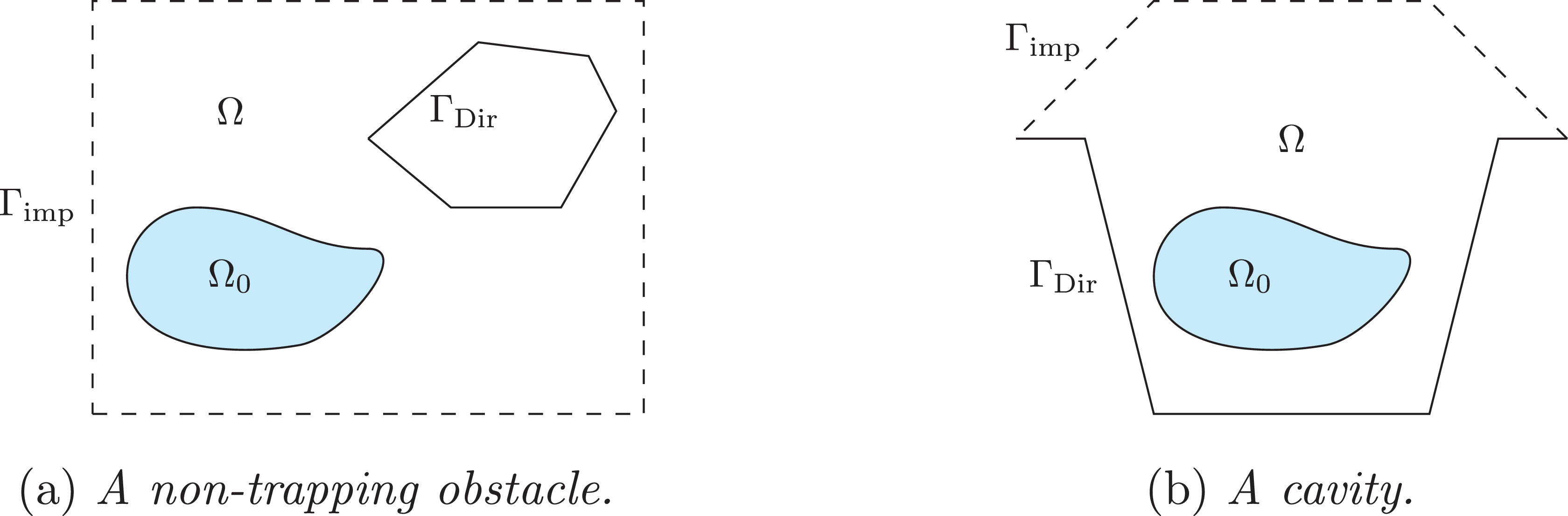

 ℜ(u)
 (12,0)
 (0,0)
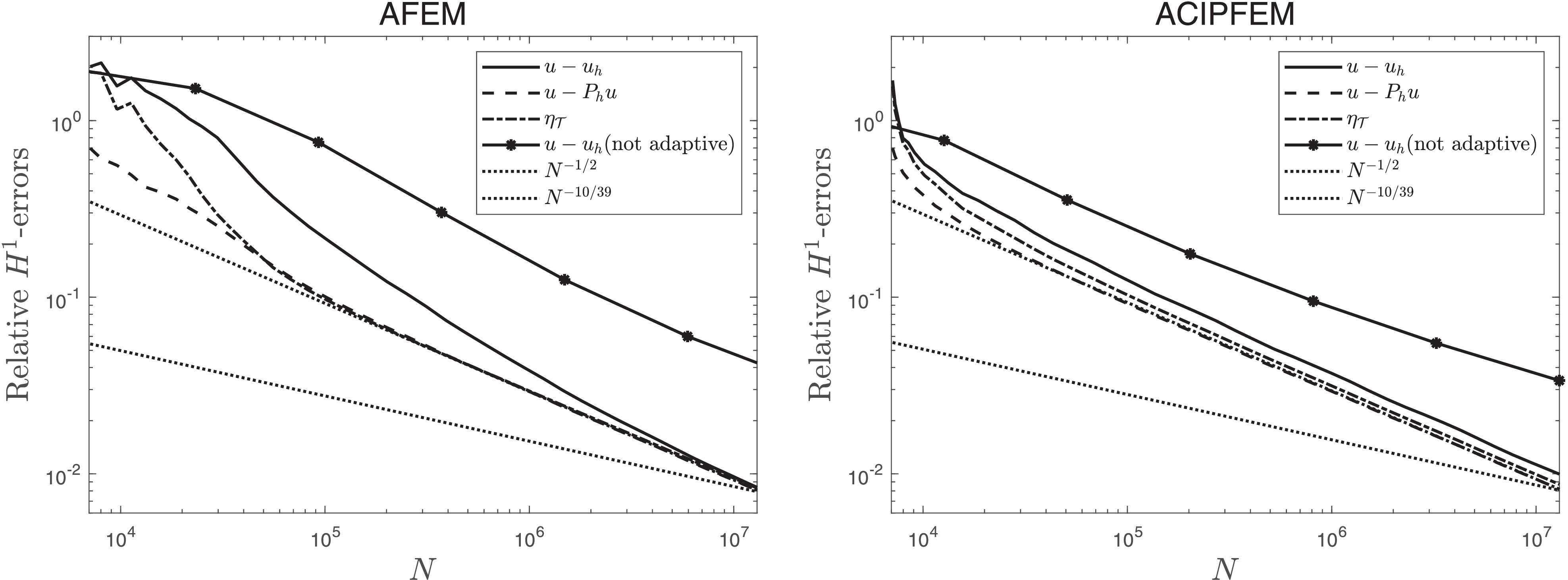
 H1
 k=80,q=20,hT0=0.04
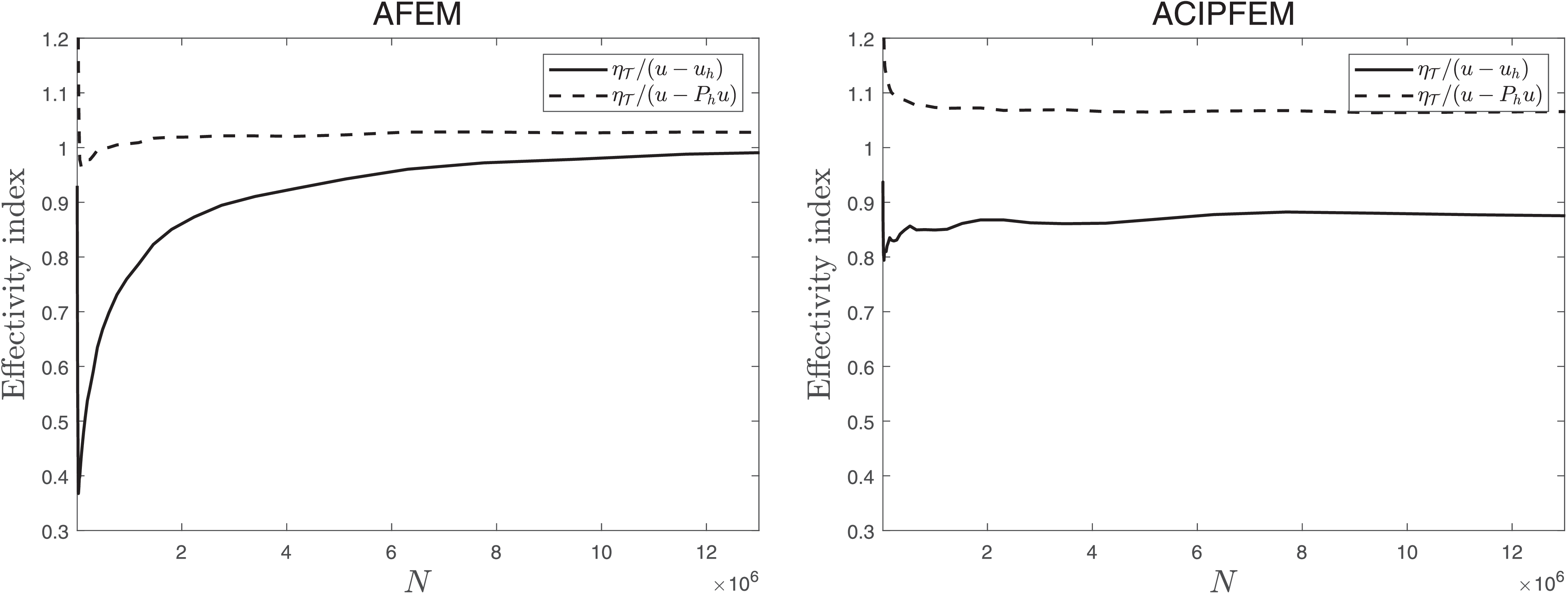
 k=80,q=20,hT0=0.04
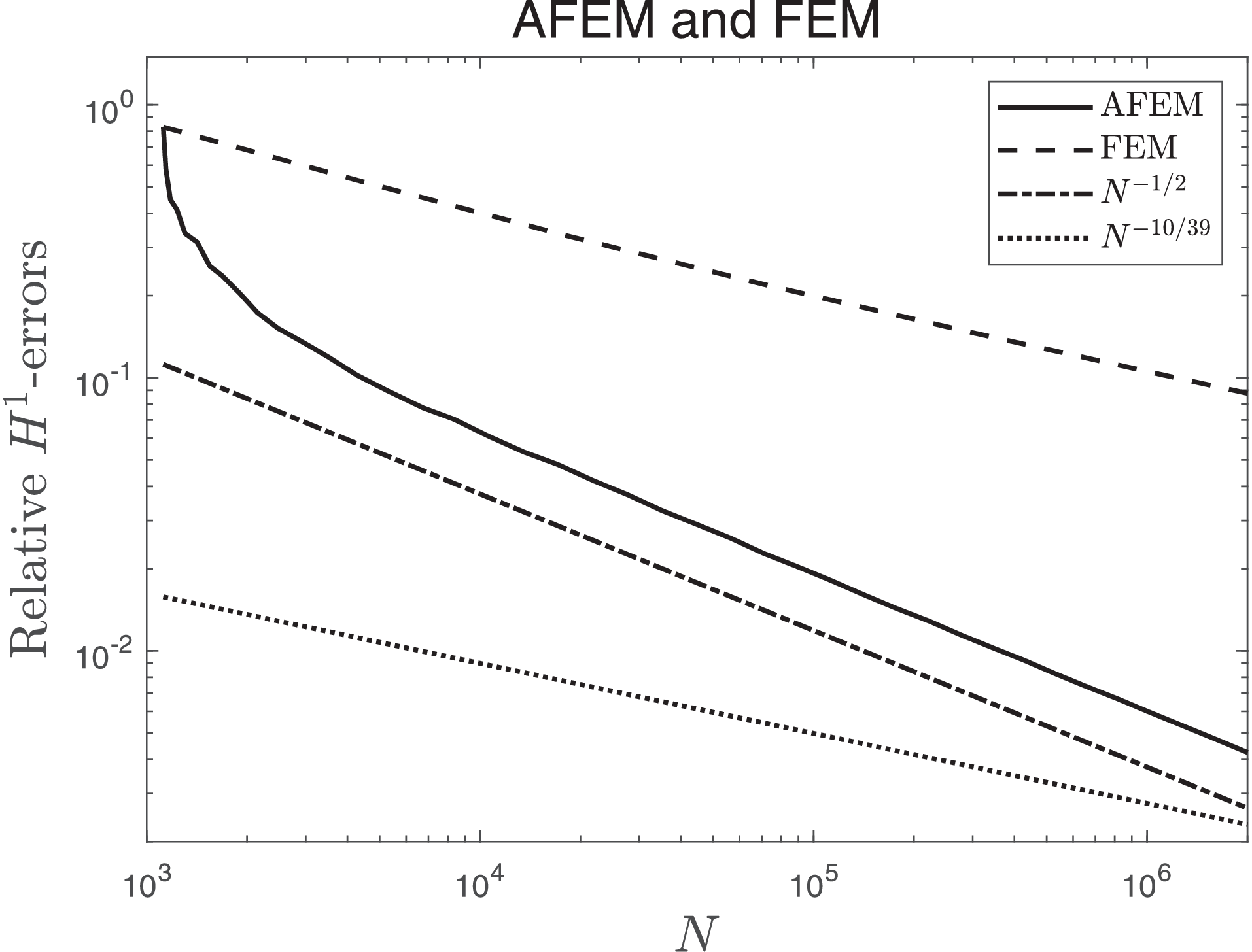
 H1
 k=5,q=1
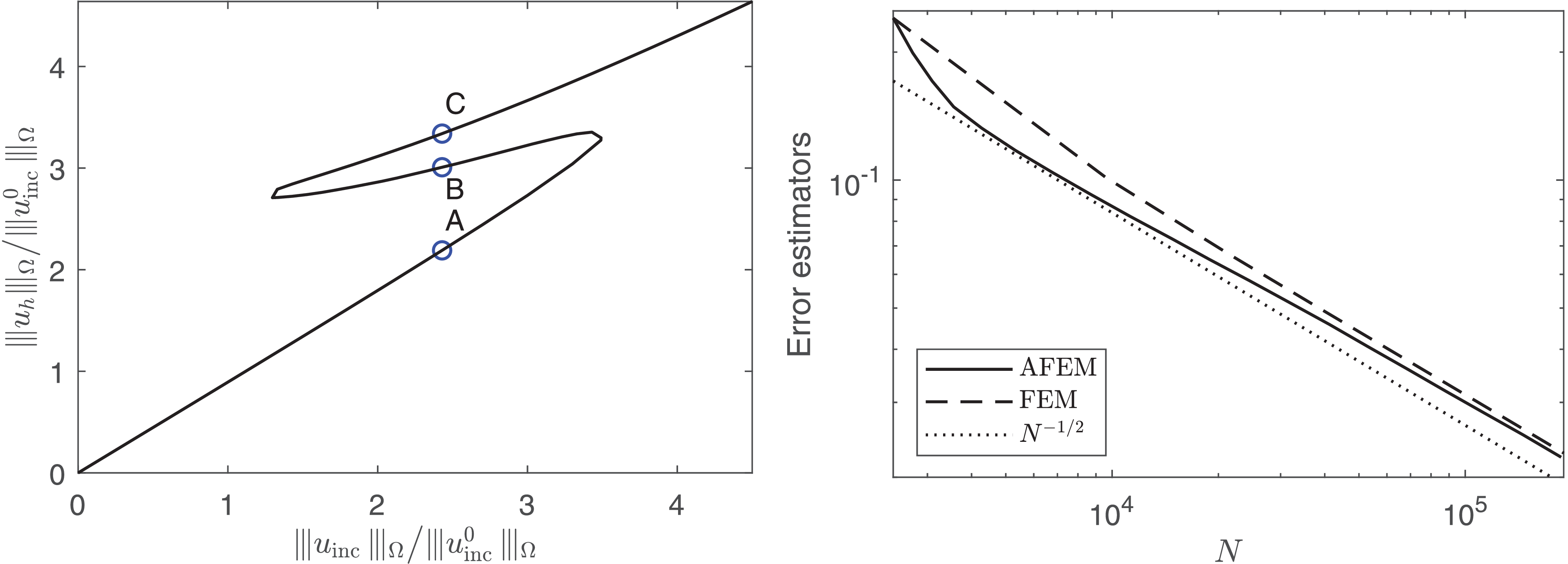
 ηT
 A


 |uh|1,T

 Open access

