
 L2
 L2





1. Introduction
Finite-size effects, where random fluctuations in agent-based systems remain non-negligible relative to the predictions of their corresponding mean-field equations, are widely observed in human-interacting and particle-interacting systems across the social and natural sciences (see, e.g., [Reference Chang, Tzou, Ward and Wei20, Reference Gomez, Ward and Wei31, Reference Hamba33, Reference Kolokolnikov, Ward, Tzou and Wei40, Reference Kolokolnikov and Wei41, Reference Paquin-Lefebvre, Nagata and Ward51, Reference Tse and Ward61, Reference Tzou, Ward and Wei62, Reference Ward63]). In an agent-based approach, the attributes of individual particles or human agents, such as their locations, velocities and states, are recorded and updated in a discrete and random manner. In contrast, mean-field equations are less granular and generally take the form of deterministic ordinary differential equations (ODEs) or partial differential equations (PDEs), offering reduced computational cost while allowing the use of classical analytical tools. The trade-off, however, is that they primarily capture the bulk and mean behaviour of the underlying agent-based system, while neglecting particle-level or individual-level heterogeneity and randomness.
This issue is particularly pronounced in epidemic modelling, since mean-field equations – built upon the inherent assumption of a well-mixed population – may fail to accurately describe epidemic dynamics in finite or heterogeneously structured populations. Indeed, extensive observations over recent decades (see e.g. [Reference Bertozzi, Franco, Mohler, Short and Sledge10, Reference Li, Wang, Li and Bertozzi44, Reference Peng, Lu, Lin, Lindstrom, Parkinson, Wang, Bertozzi and Porter53, Reference Xiong, Wang, Zhang and Britton65]) indicate that real-world epidemics have not always followed the trajectories predicted by mean-field equation models. Such deviations are particularly pronounced in restricted or localized settings with relatively small populations, where individual-level heterogeneities, including social behaviour, physical mobility and contact structures, are often disproportionately amplified. Consequently, without a clear quantitative understanding of finite-size effects in disease transmission dynamics, significant challenges arise for public health planning and policy decision-making in disease control and prevention. Despite the importance of this topic, it remains, to the best of our knowledge, largely unexplored. One of the pioneering works in this direction is [Reference Li, Wang, Li and Bertozzi44], where the authors focus on finite-size effects in epidemic regimes characterized by either the absence of an outbreak or the occurrence of a single outbreak. In this work, we extend this line of research by considering a broader range of real-world epidemic dynamical behaviours, including persistent and recurrent epidemic waves.
Epidemic waves – characterized by repeated rises and falls in infection levels – are a pervasive feature of many infectious diseases, such as recurring seasonal surges (e.g., influenza or the common cold) and major pandemic waves (e.g., COVID-19); see, for example, [Reference Cacciapaglia, Cot and Sannino17, Reference Kaxiras and Neofotistos37, Reference Mummert, Weiss, Long, Amigó, Wan and Roberts48, Reference Tang, Zhou, Wang, Wu and Xiao59]. In this intrinsically nonlinear dynamical regime, stochastic fluctuations may accumulate across successive outbreaks, making finite-size effects gradually amplified and analytically challenging. In an effort to isolate and identify finite-size effects, rather than introducing unnecessary complexity arising from overly elaborate modelling assumptions, in this article, we choose to focus on a minimal epidemic modelling framework capable of capturing disease waves. Compartmental models have long served as a foundational framework for mathematical epidemiology (see, e.g., [Reference Bertozzi, Franco, Mohler, Short and Sledge10, Reference Bongarti, Galvan, Hatcher, Lindstrom, Parkinson, Wang and Bertozzi14, Reference Liu, Mubayi, Reinhold and Zhu46]), making them a natural starting point for our modelling choice. In [Reference Li, Wang, Li and Bertozzi44], an SIR compartmental model is adopted, in which the population is divided into classes of S (susceptible), I (infectious) and R (removed). Here, in this work, we further subdivide the R compartment into H (hospitalized), R (recovered) and D (deceased) compartments, reflecting the central role of hospitalization and mortality in public health planning and risk assessment. Furthermore, we explicitly incorporate immunity waning, which allows for repeated infection cycles in the model. As a result, we arrive at an SIHRS compartmental model (with vital dynamics) in which recovered individuals may lose immunity and repeatedly become susceptible to infection upon infectious contacts.
Despite its relative simplicity, the SIHRS compartmental modelling framework, in both its agent-based and mean-field forms, exhibits rich long-term dynamical behaviour, including recurrent outbreaks across multiple settings. Moreover, without unnecessary intricacies obscuring the underlying mechanisms, this model enables us to disentangle, isolate and identify finite-size effects, shedding light on how they arise, interact with compartment structure and propagate over time. In addition, using the SIHRS compartment model as a base, one can readily incorporate a variety of elements – such as environmental and socio-economic factors – to increase the sophistication and applicability of the model. Examples include age-structured populations, complex contact networks, spatial mobility, behavioural feedback and vaccination dynamics. Each of these extensions introduces additional nonlinear couplings and new sources of randomness, creating natural opportunities to investigate how finite-size effects interact with increasingly realistic modelling features. In summary, the SIHRS model offers a flexible yet parsimonious prototype for epidemic modelling, serving as a transparent and well-structured baseline for our analysis.
Following standard agent-based formulations of compartmental epidemic models (see, e.g., [Reference Allen3, Reference Rizoiu, Mishra, Kong, Carman and Xie56]), we introduce Poisson clocks into the SIHRS framework to obtain an agent-based SIHRS model. The interarrival times between successive advancements of a Poisson clock are independently exponentially distributed random variables, with mean equal to the reciprocal of its advancing rate. Consequently, by the memoryless property of the exponential distribution, Poisson point processes are Markovian and therefore possess the memoryless property.
Particularly, in this formulation, each individual agent is equipped with independent Poisson clocks that govern the timing of events such as actions and state transitions. This construction ensures that events occur randomly in continuous time, without any prescribed ordering, and naturally generates ensembles of sample paths corresponding to distinct stochastic realizations of the epidemic dynamics. Moreover, it naturally leads to a continuous-time Markov process description of the underlying stochastic process. Exploiting this Markovian structure, we adopt a martingale approach for the agent-based SIHRS model. Specifically, we derive a martingale formulation that decomposes the stochastic dynamics into an integral term representing the infinitesimal mean and a martingale term accounting for the infinitesimal variance, following standard calculations (see, e.g., [Reference Durrett25, Reference Durrett26, Reference Kipnis and Landim39, Reference Liggett45]). Starting from this martingale formulation, we derive the associated mean-field description of the agent-based SIHRS model, which takes the form of a deterministic system of ODEs. The derivation closely parallels that of the classical hydrodynamic limit for interacting particle systems (see, e.g., [Reference Bichteler13, Reference Durrett25, Reference Durrett26, Reference Kipnis and Landim39, Reference Liggett45, Reference Mourrat47]).
To quantify the deviations between the agent-based model and its corresponding mean-field ODE system, we introduce a time-integrated
 $L^2$
discrepancy that measures the difference between stochastic and deterministic dynamics. We further apply a probabilistic decomposition that separates this discrepancy into a bias term arising from nonlinear expectations and a fluctuation term governed by the variance of the stochastic process. This decomposition yields a transparent structural interpretation of the finite-size effects. Numerical experiments indicate that both components grow as the population size decreases, resulting in dynamical behaviours – such as early die-out and irregular long-term oscillations – that arise in the agent-based model but do not appear in the deterministic counterpart. To explain these observations, we develop new techniques for deeper analysis. By combining martingale formulations with early-time asymptotic expansions, we can explicitly track the development and propagation of finite-size effects across successive time steps. For the first component, we show that initially small stochastic deviations in the infinitesimal drift can accumulate over time, leading to a systematic separation between random-path expectations and deterministic trajectories. For the second component, we demonstrate that the variance of the stochastic process admits an upper bound that scales inversely with the population size, and we provide numerical evidence suggesting that this inverse-scaling behaviour persists over a nontrivial time interval whose length may depend on both the compartment and the population size.
A key contribution of our methodology is the development of martingale formulations that extend beyond compartment variables to include higher-order interaction terms, such as the stochastic instantaneous infection rate. This extension is essential for advancing the early-time analysis beyond the initial stages and connecting early-time stochastic fluctuations with their nonlinear amplification and persistence over longer time scales. To the best of our knowledge, a martingale formulation at this higher-order level has not been developed in existing literature. While our analysis is conducted in the context of epidemic compartment models, the underlying methodology is not model-specific and may be applicable to a broader class of stochastic interacting-agent systems in which finite-size effects play a significant role. Our investigation demonstrates that finite-size effects depend not only on the total population size but also on the relative sizes of individual compartments and the temporal evolution of the system. In particular, stochastic deviations can accumulate across multiple epidemic waves, leading to sustained divergence from the mean-field dynamics. Furthermore, compartments that remain small in size, such as the hospitalized compartment, can exhibit pronounced stochastic variability even when the overall population is large.
Our theoretical analysis is supported and further complemented by an extensive suite of numerical simulations, including experiments calibrated with national-scale COVID-19 data and a focused county-level case study. For simulations informed by national-level data, we deliberately examine the agent-based SIHRS model across a wide range of population sizes, spanning regimes dominated by strong finite-size effects to regimes in which the dynamics increasingly approach those predicted by the mean-field equations. This choice enables a systematic investigation of the dependence of finite-size effects on population size. To further bridge the theoretical framework with realistic epidemic scenarios, we include a case study based on COVID-19 data from a small U.S. county whose population size is representative of many local communities. The simulations are calibrated using the county’s actual population size along with daily reported case counts and hospitalization data. Through a comparison between the real-life data, ensembles of stochastic sample paths from the agent-based model, and the corresponding mean-field trajectories, this case study provides a clear and interpretable illustration of compartment-dependent finite-size effects in realistic epidemic settings.
Overall, our findings establish a comprehensive, quantitative and analytical understanding of how finite-size effects influence the formation and evolution of epidemic dynamics, particularly in regimes characterized by recurrent epidemic waves. Specifically, the results highlight intrinsic limitations of deterministic mean-field descriptions in such settings and demonstrate that stochastic fluctuations can remain significant and continue to influence epidemic evolution even when the overall population size is relatively large.
The remainder of this paper is organized as follows. Section 2 introduces the basic assumptions of the agent-based SIHRS model, with particular emphasis on the assignment of Poisson clocks. A statistically equivalent description is then derived using Poisson merging and splitting techniques (Section 2.2), which effectively reduces the parameter set and facilitates the design of efficient simulation algorithms (Section 2.2.2). Section 4 presents the martingale-based framework. In Section 3.1, a martingale formulation is derived for each compartment variable of the agent-based SIHRS model. Based on this formulation, the corresponding mean-field equation, given by a deterministic ODE system, is obtained in Section 3.2. In Section 4, we introduce a time-integrated
 $L^2$
distance as a quantitative measurement of deviation between the agent-based and ODE models (Section 4.1) and present a probabilistic decomposition of this
 $L^2$
discrepancy into two components (Section 4.2). Further analytical, theoretical and numerical investigations focusing on these two components are presented in Sections 5 and 6, respectively. Section 7 presents a case study based on Carson City, Nevada, a small U.S. county.
The Appendix contains supplementary calculations and proofs supporting the results presented in the main text. In particular, Appendices A.1 and A.2 provide explicit calculations of the infinitesimal generators as well as a rigorous proof establishing an upper bound on the variances of the martingale terms in the martingale formulation developed in Section 2.1. In Appendix A.3.1, we present well-posedness theory together with an asymptotic analysis for the mean-field ODE system. Finally, in Appendix A.4, a martingale analysis analogous to that used for the compartment variables (Section 3) is applied to the instantaneous stochastic infection rate. In particular, a martingale formulation that separates infinitesimal mean behaviour from infinitesimal variance contributions, along with an early time-step analysis, is derived in Appendices A.4.1 and A.4.2, respectively.
The Appendix contains supplementary calculations and proofs supporting the results presented in the main text. In particular, Appendices A.1 and A.2 provide explicit calculations of the infinitesimal generators as well as a rigorous proof establishing an upper bound on the variances of the martingale terms in the martingale formulation developed in Section 2.1. In Appendix A.3.1, we present well-posedness theory together with an asymptotic analysis for the mean-field ODE system. Finally, in Appendix A.4, a martingale analysis analogous to that used for the compartment variables (Section 3) is applied to the instantaneous stochastic infection rate. In particular, a martingale formulation that separates infinitesimal mean behaviour from infinitesimal variance contributions, along with an early time-step analysis, is derived in Appendices A.4.1 and A.4.2, respectively.
2. The agent-based SIHRS model and simulations
We begin with the setup of an agent-based compartmental model, which consists of essentially two components: a cohort of individual agents who interact and subsequently evolve through varying stages of infection and recovery. In particular, agents can be assigned to five disjoint classes: Susceptible (S), Infectious (I), Hospitalized (H), Recovered (R) and Deceased (D). Here, the D compartment specifically represents individuals who have died as a consequence of the epidemic. Furthermore, we choose to exclude births from the vital dynamics, as our focus is on the transmission stages of an epidemic course. Moreover, deaths from causes unrelated to the epidemic, such as natural deaths, are also excluded.
Under this notation, S, I, H and R can be viewed as intermittent states of disease evolution, whereas the D state is permanent. Moreover, we assume that individuals in the R class may lose immunity and transition back to S. Furthermore, rather than using deterministic time steps, occurrences of individual events are governed by independent Poisson clocks. Subsequently, we will refer to this agent-based model as the SIHRS-IPC model (with vital dynamics). Here, IPC stands for Independent Poisson Clocks.
We assume a continuous time variable
 $t \in [0,\infty )$
, a probability space
 $\left (\Omega , \mathscr{F}, \mathbb{P}\right )$
, where
 $\Omega$
is the sample space,
 $\mathscr{F}$
is the associated
 $\sigma$
-algebra and
 $\mathbb{P}$
is the underlying probability measure. We then set a deterministic population size
 $N$
(which includes the deceased compartment) that is fixed in time. For each sample point
 $\omega \in \Omega$
, we assume that at a given time
 $t$
, the numbers in the five compartments are
 $\textbf {S}_N(\omega , t)$
,
 $\textbf {I}_N(\omega , t)$
,
 $\textbf {H}_N(\omega , t)$
,
 $\textbf R_N(\omega , t)$
and
 $\textbf D_N(\omega , t)$
, respectively. For every
 $t$
, we define the stochastic process
 ${\textbf {S}}_{N}(t)$
as
 $\{ {\textbf {S}}_{N}(\omega ,t)\,:\,\omega \in \Omega \}$
and similarly define
 $\textbf {I}_N(t)$
,
 $\textbf {H}_N(t)$
,
 $\textbf {R}_N(t)$
and
 $\textbf {D}_N(t)$
. Thus, for every
 $t$
, we have
 \begin{equation} N =\textbf {S}_N( t)+\textbf {I}_N( t)+\textbf {H}_N( t)+\textbf {R}_N(t)+\textbf {D}_N( t). \end{equation}
Moreover, we assume that the initial data are deterministic (but may depend on
 $N$
) and are denoted by
 $ {S}_{0N}$
,
 $ {I}_{0N}$
,
 ${H}_{0N}$
,
 ${R}_{0N}$
and
 ${D}_{0N}$
.
2.1. Event occurrences driven by independent Poisson clocks
We assume that the evolution of an agent’s state during the course of an epidemic may involve transitions among the five compartments, associated with infectious contact, hospitalization, recovery, immunity waning and death. In particular, susceptible agents may transition to the infectious state; infectious agents may transition to any other state except susceptible; hospitalized agents may transition to the recovered or deceased states; recovered agents may lose immunity and return to the susceptible class and deceased agents remain permanently in the D compartment.
We employ several types of Poisson clocks ( Type (I) – Type (IV) ) to model events associated with these stages, assuming that all clocks advance independently. Each clock advances according to a Poisson process with a specified rate; therefore, the waiting times between events are independent, exponentially distributed random variables with means equal to the reciprocals of the corresponding rates. Poisson processes are a fundamental modelling tool in many fields, such as chemistry and physics (see, e.g., [Reference Bertero, Boccacci, Desiderà and Vicidomini9, Reference Citi, Ba, Brown and Barbieri22, Reference Embrechts, Frey and Furrer28, Reference Erban and Chapman29]).
We note that the four Poisson clock types introduced below are intended to describe the biological mechanisms of disease progression rather than the final computational representation of the stochastic process. As pointed out in the stochastic simulation literature (see, e.g., [Reference Erban and Chapman29]), one may equivalently begin directly with the effective transition clocks obtained after Poisson thinning, leading immediately to the Gillespie stochastic simulation algorithm. Later, Section 2.2 serves this purpose; it demonstrates how the biologically motivated formulation can be systematically transformed, through the classical Poisson splitting and merging properties, into an equivalent Gillespie-type formulation consisting only of effective transition clocks.
Type (I)
Poisson clocks govern contacts between susceptible (S) and infectious (I) individuals. Specifically, each
 $(S,I)$
pair is assigned a
Type (I)
clock with an advancing rate
 $\beta /N$
, where
 $\beta \gt 0$
does not depend on
 $N$
(note that all parameters of the SIHRS-IPC model are assumed to be independent of
 $N$
, unless otherwise stated). Upon an advancement of a
Type (I)
clock at time
 $t^{-}$
, at time
 $t$
, the corresponding susceptible agent either transitions to state I with probability
 $p_{SI}$
or remains in state S with probability
 $1-p_{SI}$
(the subscripts in each probability indicate the initial and subsequent states of an agent). Moreover, we assume that
 $p_{SI}\in [0,1]$
, which holds for all transition probabilities throughout.
Each agent in the infectious state is assigned a
Type (II)
Poisson clock with an advancing rate
 $\gamma$
. A
Type (II)
Poisson clock governs transitions with four possible outcomes depending on symptom severity: direct recovery without hospitalization (typically asymptomatic or mild cases), persistence in the infectious state, hospitalization (typically severe cases) and direct death without hospitalization. More precisely, upon an advancement of a
Type (II)
clock, the clock transitions to state
 $H$
,
 $R$
or
 $D$
with probabilities
 $p_{IH}$
,
 $p_{IR}$
and
 $p_{ID}$
, respectively, or remains in state
 $I$
with probability
 $p_{II}=1-p_{IH}-p_{IR}-p_{ID}$
.
A
Type (III)
clock with rate
 $\alpha$
is assigned to each agent in state H to govern outcomes of hospitalization. Upon an advancement, the carrier either transitions to state R with probability
 $p_{HR}$
or to state D with probability
 $p_{HD}$
or remains in state H with probability
 $p_{HH}=1-p_{HR}-p_{HD}$
.
Transitions at the stage of immunity waning are governed by
Type (IV)
clocks with rate
 $\lambda _{RS}$
. Each agent in state R is assigned a
Type (IV)
clock, and upon its advancement, the agent loses immunity and transitions back to the Susceptible state.
For the reader’s convenience, we list the state transitions governed by each type of Poisson clock in Table 1.
Poisson clocks and their associated state transitions

Table 1. Long description
The table presents state transitions for four types of Poisson clocks. It has four columns labeled Type (I), Type (II), Type (III), and Type (IV). Each column lists a specific state transition. Type (I) shows S transitioning to I, S. Type (II) shows I transitioning to H, R, D, I. Type (III) shows H transitioning to R, D, H. Type (IV) shows R transitioning to S.
2.2. A statistically equivalent description of the SIHRS-IPC model
By implementing merged and split Poisson processes, we derive a statistically equivalent description of the agent-based SIHRS-IPC model, which significantly facilitates computer simulation. To the best of our knowledge, although such ideas are anecdotally known, detailed and fully explicit constructions of statistically equivalent descriptions for agent-based compartmental models of this level of complexity appear to be relatively scarce in the existing literature. A related approach has been considered in simpler settings, such as [Reference Li, Wang, Li and Bertozzi44], where the underlying model is of SIR compartmental type.
Poisson merging and splitting are basic properties of Poisson processes (see, e.g., [Reference Durrett26]); for additional explanations, see Remark 1 below. Roughly speaking, a Poisson process whose arrivals are categorized into different groups is equivalent to a collection of independent split Poisson processes whose arrival rates are equal to the rate of the original process multiplied by the corresponding grouping probabilities. At the same time, independent Poisson processes associated with Poisson clocks can be treated as a single merged Poisson process, in which the clocks “compete” to advance first, with probabilities proportional to their respective rates.
2.2.1. Application of Poisson splitting and merging
We first use Poisson splitting to obtain thinned, effective Poisson clocks, upon whose advancements exactly one type of transition between states occurs (i.e., with probability one). We then merge each type of thinned clock to obtain master clocks and finally merge all master clocks into a single clock governing the occurrences of all effective transitions.
Each
Type (I)
clock can be split into two clocks: an “effective” clock that governs contacts leading to a transition between the S and I compartments, and another clock that corresponds to non-infectious contacts. The effective Type (I) clock has advancing rate
 $p_{SI}\beta /N$
. In a similar way, each
Type (II)
and
Type (III)
clock can be split into four and three thinned clocks, respectively. Among these seven types of clocks, the effective ones are those governing transitions from I to H, I to R, I to D, H to R and H to D; their advancing rates are
 $p_{IH} \gamma$
,
 $p_{IR} \gamma$
,
 $p_{ID} \gamma$
,
 $p_{HR} \alpha$
and
 $p_{HD} \alpha$
, respectively. We note that there is no need to split any
Type (IV)
clocks.
As all effective clocks remain independent Poisson clocks (see Remark 1), we apply Poisson merging to each type of effective clocks. By merging all effective Type (I) clocks, we obtain a master effective Type (I) clock with rate
 $\beta _{SI} \textbf {I}_N ( t) \textbf {S}_N( t) / N$
because
 $\textbf {I}_N ( t) \textbf {S}_N( t)$
is the raw count of
 $(I,S)$
pairs at time
 $t$
. Similarly, the rates of the master effective clocks governing transitions from I to R, I to D and I to H, from H to D and H to R and from R to S are given by
 $p_{IR}\gamma \textbf {I}_{N}( t)$
,
 $p_{ID}\gamma \textbf {I}_{N}( t)$
,
 $p _{IH}\gamma \textbf {I}_{N}( t)$
,
 $p_{HD}\alpha H_{N}( t)$
,
 $p_{HR}\alpha H_{N}( t)$
and
 $\lambda _{RS} {R}_{N} ( t)$
, respectively. Based on this observation, we note that there is no loss in reducing the parameter set by permanently combining certain pairs of parameters. Table 2 lists the parameters that are combined and renamed to reduce the size of the parameter set.
Renaming of parameters for reducing the effective parameter set of the SIHRS-IPC model

Table 2. Long description
Panel A: The table lists original parameters and their renamed versions. The original parameters include pSIβ, pHIγ, pIRγ, pIDγ, pHRα, and pHDα. The renamed parameters are βSI, γIH, γIR, γID, αHR, and αHD respectively. The table aims to reduce the effective parameter set of the SIHRS-IPC model by combining certain pairs of parameters.
Finally, by applying Poisson merging to the seven master clocks obtained above, we obtain a single “sovereign” clock that governs the arrivals of all effective transitions. The advancing rate of the sovereign effective clock, denoted by
 ${\Lambda }_N( t)$
, is given by the sum of the rates of the seven master clocks
 \begin{align} \quad {\Lambda }_N( t) & =\dfrac {\beta _{SI}\textbf {I}_N ( t) \textbf {S}_N( t)}{N} + \left (\gamma _{IH} + \gamma _{IR} + \gamma _{ID} \right) \textbf {I}_{N}( t) + ( \alpha _{HR} + \alpha _{HD}) \textbf {H}_{N}( t) +\lambda _{RS}\textbf {R}_{N} ( t). \end{align}
Remark 1.
In general, suppose
 $X(t)$
is a Poisson process with arrival rate
 $\Lambda$
, and that each arrival is independently assigned to the
 $k$
-th process, denoted by
 $X_k(t)$
, with probability
 $p_k$
, for
 $k=1,2,\ldots ,m$
. As a result, we obtain the stochastic processes
 $X_1(t),\ldots ,X_m(t)$
. These processes are independent Poisson processes, with arrival rates
 $\Lambda _k =\Lambda p_k$
,
 $k=1,\ldots ,m$
.
Conversely, starting with multiple independent Poisson processes
 $X_1(t),\ldots ,X_m(t)$
with arrival rates
 $q_1,q_2,\ldots ,q_m$
, respectively, we can merge them into a single Poisson process with an advancing rate
 $\sum _{n=1}^{m} q_n$
. That is, the sum
 $\sum _{k=1}^{m} X_k(t)$
has the same distribution as the number of arrivals of a Poisson process with rate
 $\sum _{k=1}^{m} q_k$
. Furthermore, each arrival of the merged process originates from the
 $k$
-th process with probability
 $q_k / \sum _{n=1}^{m} q_n$
, for
 $k=1,2,\ldots ,m$
, independently of all other arrivals and their origins.
2.2.2. An equivalent description based on the merged clock
Once the sovereign clock is established, we can provide an equivalent description of the SIHRS-IPC model. Upon an advancement of the sovereign clock at time
 $t^{-}$
, exactly one transition occurs at time
 $t$
among the seven possible transitions: from S to I; from I to R, H or D; from H to R or D and from R to S. The corresponding transition probabilities are determined by the ratios of the rates of the associated master clocks to
 ${\Lambda }_N( t)$
, as summarized in Table 3.
The probabilities corresponding to transitions from S to I; from I to R, H, or D; from H to R or D; and from R to S, written in terms of the reduced parameter set of the SIHRS-IPC model

Table 3. Long description
A table titled `Table 3' displays the probabilities corresponding to various transitions in the SIHRS-IPC model. The table has two rows and seven columns. The first row lists the transitions: S to I, I to R, I to H, I to D, H to R, H to D, and R to S. The second row provides the probabilities for each transition, written in terms of the reduced parameter set of the SIHRS-IPC model. The probabilities are as follows: Row 1: S to I, I to R, I to H, I to D, H to R, H to D, R to S. Row 2: beta sub S I N sub I (t) S sub N (t) divided by N sub Lambda N (t), gamma sub I R I sub N (t) divided by Lambda N (t), gamma sub I H I sub N (t) divided by Lambda N (t), gamma sub I D I sub N (t) divided by Lambda N (t), alpha sub H R H sub N (t) divided by Lambda N (t), alpha sub H D H sub N (t) divided by Lambda N (t), lambda sub R S R sub N (t) divided by Lambda N (t).
Figure 1 provides a schematic overview of the SIHRS-IPC model, illustrating the evolution of the compartment classes together with the associated transition mechanisms and probabilities.
Diagram summarizing an equivalent description of the SIHRS-IPC model with a reduced set of parameters.

Based on the equivalent description derived above, it follows immediately that the disease-free and death-free homogeneous equilibrium of the SIHRS-IPC system is given by
 \begin{equation} ( N, 0, 0, 0, 0). \end{equation}
Furthermore, Table 3 shows that the parameter
 $\beta _{SI}$
plays the role of the effective transmission rate, whereas the combined rate
 $\gamma _{IR} + \gamma _{ID} + \gamma _{IH}$
represents the total removal rate from the infectious compartment, accounting for recovery, hospitalization and death. Thus, we obtain an estimate of the basic reproduction number R
 $_0$
as the ratio
 \begin{equation} \mbox{R$_0$} =\dfrac {\beta _{SI}} { \gamma _{IR} + \gamma _{ID} + \gamma _{IH} }. \end{equation}
Moreover, the equivalent description derived above provides a simulation method with significantly reduced computational time and effort, namely the Gillespie algorithm (see, e.g., [Reference Gillespie30]). The advantage of this simulation method is that it avoids the requirement of individual Poisson clocks to advance sequentially according to a prescribed diagram. One can first generate the current sojourn time of the single sovereign effective clock with rate
 $ {\Lambda }_N( t)$
, as in Eq. (2.2), using an exponential distribution and then determine which transition occurs by sampling from the probabilities listed in Table 3. Consequently, we can generate sample paths corresponding to random realizations of event sequences without any pre-determined ordering.
Remark 2.
We note that, with the equivalent description of the SIHRS-IPC model developed above, we can introduce the concept of a possible blow-up time for the associated stochastic process. It is possible that, for a given realization of the SIHRS-IPC model, the Poisson clocks generate time increments whose sum is finite, that is,
 $\tau \lt \infty$
. In this case, the corresponding stochastic process is defined only for
 $0\leq t \lt \tau$
. At time
 $t=\tau$
, the Poisson clocks produce an infinite number of advances. We then say that the stochastic process explodes and
 $\tau$
is called the blow-up time.
2.3. Numerical simulations of the SIHRS-IPC model
We perform simulations of the SIHRS-IPC model for a wide range of total population sizes
 $N$
, which are frequently encountered in small-scale population regions in real life. To observe the full effects of immunity waning (over approximately a three-month period), we set the ending time of the simulations to
 $1000$
days. The results are displayed in Figures 2 and 3, showing single random sample paths and path averages, respectively.
Output of the compartment fractions of the SIHRS-IPC model for different values of
 $N$
from time
 $0$
to
 $1000$
days. The S, I, H, R,and D compartments are displayed using golden yellow, purple, dark green, teal and navy curves, respectively. They are grouped into three sets:
 $( \mathbf {s}_N( t) , \mathbf {r}_N( t))$
,
 $( \mathbf {i}_N( t) , \mathbf {d}_N( t) )$
and
 $\mathbf {h}_N( t)$
, shown in the left, middle and right columns, respectively. In the first, second, third and fourth rows, we set
 $N=550$
,
 $1300$
,
 $2900$
and
 $7000$
, respectively. For all panels, the initial conditions at
 $t=0$
are set to
 $s_{0N}=0.96$
,
 $i_{0N}=0.035$
and
 $h_{0N}=0.005$
, and the parameters are chosen as listed in Table 4
.

Figure 2. Long description
The image contains twelve line graphs organized into four rows and three columns. Each row represents different values of N, with the first row for N = 550, the second row for N = 1300, the third row for N = 2900, and the fourth row for N = 7000. The columns represent different compartments of the SIHRS-IPC model. Panel A, D, G, and J in the first column show the fractions of susceptible (S) and recovered (R) compartments over time. The x-axis is labeled Time (days), and the y-axis is labeled s N(t), r N(t). Panel B, E, H, and K in the second column show the fractions of infected (I) and dead (D) compartments over time. The x-axis is labeled Time (days), and the y-axis is labeled i N(t), d N(t). Panel C, F, I, and L in the third column show the fraction of hospitalized (H) compartment over time. The x-axis is labeled Time (days), and the y-axis is labeled h N(t). Each graph displays trends over a period of 1000 days. The colors used in the graphs are golden yellow for S, purple for I, dark green for H, teal for R, and navy for D. The initial conditions and parameters are consistent across all panels as listed in Table 4 of the referenced study.
Output of the random path averages of the compartment fractions of the SIHRS-IPC model for different values of
 $N$
from time
 $0$
to
 $1000$
days. In panel (a), the averaged output of 70 random paths with the same parameters and initial data as in panel (a) of Figure 2
is displayed. The same convention applies to all other panels. The S, I, H, R and D compartments are displayed using golden yellow, purple, dark green, teal and navy curves, respectively.

2.3.1. Parameter choices
The parameters are chosen according to the characteristics of the COVID-19 pandemic, with an emphasis on U.S. data. All the parameter values are listed in Table 4.
Parameter values for the SIHRS-IPC model simulations

Table 4. Long description
A table listing parameter values for a model simulation. The table has two rows and seven columns. The first row contains the column headers: Parameters and Values. The second row lists the parameter names and their corresponding values. The parameters are beta subscript S I, gamma subscript H H, gamma subscript I R, gamma subscript H D, alpha subscript H R, alpha subscript H D, and lambda subscript R S. The values for these parameters are 0.213881786, 0.010204286, 0.11836714285, 0, 0.094, 0.017111, and 0.008134 respectively.
Regarding the parameters
 $\gamma _{IH}$
,
 $\gamma _{IR}$
and
 $\gamma _{ID}$
, Table 2 indicates that it is sufficient to estimate the total transition rate
 $\gamma$
together with the branching probabilities
 $p_{IH}$
,
 $p_{IR}$
and
 $p_{ID}$
. We choose
 $\gamma$
to be the inverse of
 $7$
days, which is consistent with the mean time interval from infectious contact through symptom onset to hospital admission, based on surveillance studies of COVID-19–like respiratory diseases (see, e.g., [Reference Lauer, Grantz, Bi, Jones, Zheng, Meredith, Azman, Reich and Lessler43]). We set
 $p_{IH}=0.07143$
according to U.S.-based analyses [Reference Deng, Kim, Bratcher, Jones, Simuzingili, Gundlapalli, Hagen, Iachan and Clarke24], which suggests that
 $p_{IH}$
for adults typically ranges from
 $0.04$
to
 $0.08$
. For
 $p_{ID}$
, we note that out-of-hospital deaths represent only a small fraction of total deaths (see, e.g., [Reference O’Driscoll, Ribeiro Dos Santos, Wang, Cummings, Azman, Paireau, Fontanet, Cauchemez and Salje50, Reference Pathak, Garcia, Menard and Salemi52]); therefore, we set
 $p_{ID}=0$
. Finally, we choose
 $p_{II}=0.1$
based on virological and epidemiological studies of individuals with mild or moderate COVID-19 who are not hospitalized (see, e.g., [Reference Boucau, Marino, Regan, Uddin, Choudhary, Flynn, Chen, Stuckwisch, Mathews, Liew, Singh, Lipiner, Kittilson, Melberg, Li, Gilbert, Reynolds, Iyer, Chamberlin, Vyas, Goldberg, Vyas, Li, Lemieux, Siedner and Barczak15, Reference Cevik, Kuppalli, Kindrachuk and Peiris18, Reference Puhach, Meyer and Eckerle54]). Therefore, we obtain
 $p_{IR} = 1- p_{IH} - p_{ID}-p_{II} = 0.82857$
. Consequently,
 $\gamma _{IH}$
,
 $\gamma _{IR}$
and
 $\gamma _{ID}$
are obtained by multiplying
 $\gamma$
with
 $p_{IH}$
,
 $p_{IR}$
and
 $p_{ID}$
, respectively.
We now estimate the transmission rate
 $\beta _{SI}$
. From Eq. (2.4), we obtain
 \begin{equation*} \beta _{SI} =\mbox{R$_0$}\left (\gamma _{IR} + \gamma _{ID}+\gamma _{IH}\right ) \approx 0.1285714\mbox{R$_0$} . \end{equation*}
Consequently, the determination of
 $\beta _{SI}$
amounts to selecting an appropriate value of the basic reproduction number
 $R_0$
. Following [Reference Sy, White and Nichols58], we adopt the median reproduction number computed across 1,151 U.S. counties, namely
 $R_0 = 1.663525$
.
For the choice of
 $\alpha _{HR}$
and
 $\alpha _{HD}$
, Table 3 shows that it is sufficient to estimate
 $\alpha$
,
 $p_{HR}$
and
 $p_{HD}$
. We choose
 $\alpha$
to be the inverse of
 $9$
days, which is consistent with the reported lengths of hospital stay for COVID-19 patients (see, e.g., [Reference Alimohamadi, Mansouri Yekta, Sepandi, Sharafoddin, Arshadi and Hesari2, Reference Kapinos, Peters, Murphy, Hohmann, Podichetty and Greenberg36]). In particular, we consider the average length of stay across non-ICU and ICU cases to be
 $9$
days. For the choice of
 $p_{HD}$
, the probability of death among hospitalized patients, we set
 $p_{HD}=0.154$
based on the CDC National Hospital Care Survey [49]. As for
 $p_{HH}$
, we set it to zero, since multiple virological studies indicate that viable SARS-CoV-2 cannot be recovered from respiratory samples of hospitalized patients beyond approximately 8–10 days after symptom onset (see, e.g., [Reference Bullard, Dust, Funk, Strong, Alexander, Garnett, Boodman, Bello, Hedley, Schiffman, Doan, Bastien, Li, Van Caeseele and Poliquin16, Reference Cevik, Tate, Lloyd, Maraolo, Schafers and Ho19, Reference Wölfel, Corman, Guggemos, Seilmaier, Zange, Müller, Niemeyer, Jones, Vollmar, Rothe, Hoelscher, Bleicker, Brünink, Schneider, Ehmann, Zwirglmaier, Drosten and Wendtner64]). Consequently, we obtain
 $p_{HR} = 1 - p_{HD} - p_{HH} = 1-0.154 = 0.846$
.
Finally, we choose the immunity waning rate
 $\lambda$
based on a mean immunity period of approximately four months, or
 $122$
days, that is,
 ${1}/{\lambda } =122$
, which reflects the observed duration of natural immunity against COVID-19 (see [Reference Berber and Ross7] and [Reference Krutikov, Palmer, Tut, Fuller, Azmi, Giddings, Shrotri, Kaur, Sylla, Lancaster, Irwin-Singer, Hayward, Moss, Copas and Shallcross42]).
2.3.2. Initial data choices
Rather than raw numbers, we display the fractions of each compartment, which are denoted as follows:
 \begin{align} \left ( \textbf {s}_N( t), \textbf {i}_N( t), \textbf {h}_N( t),\textbf {r}_N( t), \textbf {d}_N( t) \right ) \,:\!=\, \dfrac {1}{N} \left ( \textbf {S}_N( t), \textbf {I}_N( t), \textbf {H}_N( t),\textbf {R}_N( t), \textbf {D}_N( t) \right )\! . \end{align}
where the corresponding initial data are denoted by
 \begin{equation} \left (s_{0N} , i_{0N}, h_{0N}, r_{0N}, d_{0N} \right ) \,:\!=\, \dfrac {1}{N} \left ( {S}_{0N}, {I}_{0N}, {H}_{0N}, {R}_{0N}, {D}_{0N} \right )\! . \end{equation}
In Figures 2 and 3, simulations are performed for total population sizes
 $N=550$
,
 $1300$
,
 $2900$
and
 $7000$
, as shown from top to bottom in the four rows. The initial data are chosen as a small perturbation of the disease-free and death-free equilibrium Eq. (2.3), with a negligible fraction of infectious and hospitalized agents. As a result, we assume that the initial data remain fixed for all choices of
 $N$
, namely,
 \begin{equation} \left ( s_{0N}, i_{0N}, h_{0N}, r_{0N}, d_{0N} \right ) \equiv \left ( 0.96, 0.035, 0.005, 0, 0 \right )\!. \end{equation}
We group compartments of comparable magnitude into three categories: susceptible and recovered, infectious and deceased and hospitalized, which are shown in the left, middle and right columns of Figures 2 and 3, respectively. In all panels, the S, I, H, R and D compartments are depicted by golden yellow, purple, dark, green, teal and navy curves, respectively. Moreover, panel (a) in Figure 2 displays a single representative random path, while panel (a) in Figure 3 reports the average of 70 random paths generated with identical parameters and initial conditions. This convention is used for all panels in Figures 2 and 3.
2.3.3. Dynamical behaviours observed in agent-based simulations
Figures 2 and 3 illustrate three qualitatively distinct dynamical regimes exhibited by the SIHRS-IPC model. The first regime corresponds to early die-out, in which stochastic fluctuations dominate and the epidemic quickly becomes extinct before sustained transmission can occur. The second regime consists of long-term oscillatory dynamics with rough trajectories, where persistent epidemic waves are present but exhibit strong stochastic variability. The third regime features long-term oscillations with smooth trajectories, where stochastic fluctuations are relatively weak. In general, these three dynamic regimes arise sequentially as
 $N$
increases. We also note that the five compartments may display different behaviours for the same value of
 $N$
. In particular, the S and R compartments tend to transition more rapidly than the I and H compartments as
 $N$
increases.
To better understand the underlying dynamic behaviour, we begin by examining the single-path realizations presented in Figure 2. For relatively small population sizes, specifically
 $N\in (0,1300)$
, the infectious fraction
 $\textbf {i}_N (t)$
typically enters the early die-out regime, remaining positive for only a short duration before vanishing, as illustrated in panels (b) and (e). Because of the strong coupling between infection and hospitalization, early die-out of
 $\textbf {i}_N (t)$
typically induces early die-out of the hospitalized fraction
 $\textbf {h}_N(t)$
, as illustrated in panels (c) and (f) of Figure 2. As the population size increases beyond this range, the system transitions into a persistent oscillatory regime. For
 $N \geq 2900$
, all five compartments display long-term oscillations without extinction. In this regime, the infectious and hospitalized fractions,
 $\textbf {i}_N (t)$
and
 $\textbf {h}_N (t)$
, exhibit sustained oscillations characterized by sharp peaks and irregular fluctuations, indicating that stochastic effects remain significant. In contrast, the susceptible and recovered fractions,
 $\textbf {s}_N (t)$
and
 $\textbf {r}_N (t)$
evolve more smoothly over time. This mixed behaviour highlights the compartment-dependent nature of finite-size effects and is clearly visible in the third and fourth rows of Figure 2.
We now compare these results with the path-averaged dynamics shown in Figure 3. Two notable differences emerge. First, averaging across multiple realizations delays the apparent die-out of both the infectious and hospitalized compartments. This effect can be observed by comparing panels (b), (c), (e) and (f) in Figure 2 with their averaged counterparts. Second, the averaged trajectories are substantially smoother than the individual sample paths, particularly in the oscillatory regimes shown in the third and fourth rows. This smoothing effect reflects the cancellation of random fluctuations across realizations while still preserving the underlying oscillatory structure driven by immunity waning and reinfection.
In summary, these observations demonstrate that finite-size effects manifest not only through dependence on population size but also through compartment-specific sensitivity to stochastic fluctuations and through differences between single-path and ensemble-averaged behaviour. In the following section, we apply a martingale-based approach to conduct a preliminary theoretical investigation of these finite-size effects.
3. A martingale approach
We derive a martingale formulation associated with the SIHRS-IPC model, as it is a continuous-time Markov pure jump process. This formulation naturally yields the associated deterministic ODE system as the mean-field equation of the SIHRS-IPC model, while simultaneously providing a probabilistic framework for quantifying finite-size deviations. Within this framework, we can establish explicit quantitative connections between the population size, compartment structure and stochastic fluctuations.
3.1. A martingale formulation
We define the vectors
 $\overrightarrow {\textbf {m}_N(t)} = \left ( \textbf {s}_N( t),\textbf {i}_N( t), \textbf {h}_N( t), \textbf {r}_N( t), \textbf {d}_N( t) \right )$
and
 $\overrightarrow { {m}_{0N}} = \left ( s_{0N}, i_{0N}, h_{0N},r_{0N}, d_{0N} \right )$
. Because
 $\overrightarrow {\textbf {m}_N(t)}$
, with the initial condition
 $\overrightarrow { {m}_{0N}}$
, is a Markov pure-jump process taking values in
 $\mathbb{R} ^5$
; therefore, a martingale formulation can be derived as follows:
Theorem 3.
For each fixed
 $N$
, before the possible blow-up time (see Remark 2), we can write
 $\overrightarrow {\textbf {m}_N(t)}$
as the following martingale formulation:
 \begin{equation} \begin{aligned} {\textbf {m}^{(l)}_N(t)} = {m^{(l)}_{0N}} + \int _{0}^{t} {\mathscr{G}^{\kern1pt(l)} \left( \overrightarrow {\textbf {m}_N(w)} \right) } dw + {\mathscr{M}^{\kern1.6pt(l)}_{N} \left( \overrightarrow {\textbf {m}_N(t)} \right) }, \quad l =1, 2, 3, 4, 5, \end{aligned} \end{equation}
where
 ${\textbf {m}^{(l)}_N(t)}$
and
 $ {m^{(l)}_{0N}}$
are the components of vectors
 $\overrightarrow {\textbf {m}_N(t)}$
and
 $\overrightarrow { {m}_{0N}}$
, respectively. The processes
 $ \mathscr{M}^{\kern1.6pt(l)}\left( \overrightarrow {\textbf {m}_N(t)} \right)$
are martingales starting from zero at
 $t=0$
, and
 $ \mathscr{G}^{\kern1pt(l)}\left( \overrightarrow {\textbf {m}_N(t)} \right)$
denote the infinitesimal means of
 $ {\textbf {m}^{(l)}_N(t)}$
,
 $ l = 1, 2, 3, 4, 5$
, given by
 \begin{equation} \begin{cases} \mathscr{G} ^{\kern1.3pt(1)} \left( \overrightarrow {\textbf {m}_N(t)} \right) = -\beta _{SI} \textbf s_N(t) \textbf i_N(t) + \lambda _{RS} \textbf r_N(t) , \\[3pt] \mathscr{G} ^{\kern1.3pt(2)} \left( \overrightarrow {\textbf {m}_N(t)} \right) = - ( \gamma _{IH}+\gamma _{IR}+\gamma _{ID}) \textbf i_N(t) + \beta _{SI} \textbf s_N(t) \textbf i_N(t) , \\[3pt] \mathscr{G} ^{\kern1.3pt(3)} \left( \overrightarrow {\textbf {m}_N(t)} \right) = \gamma _{IH} \textbf i_N(t) - \left ( \alpha _{HR} + \alpha _{HD} \right ) \textbf h_N(t), \\[3pt] \mathscr{G} ^{\kern1.3pt(4)}\left( \overrightarrow {\textbf {m}_N(t)} \right) = \gamma _{IR} \textbf i_N(t) + \alpha _{HR} \textbf h_N(t) - \lambda _{RS} \textbf r_N(t), \\[3pt] \mathscr{G} ^{\kern1.3pt(5)}\left( \overrightarrow {\textbf {m}_N(t)} \right) = \gamma _{ID}\textbf i_N(t) + \alpha _{HD}\textbf h_N(t) . \end{cases} \end{equation}
The variances of the martingales
 $ \mathscr{M}^{\kern1.6pt(l)} \left( \overrightarrow {\textbf {m}_N(t)} \right)$
, denoted as
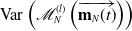 ${\operatorname {Var}}\left(\mathscr{M}_{N}^{\kern1.3pt(l)}\left( \overrightarrow {\textbf {m}_N(t)} \right) \right)$
for
 $l=1,2,3,4,5$
, satisfy
 \begin{equation} {\operatorname {Var}}\left(\mathscr{M}_{N}^{\kern1.3pt(l)}\left( \overrightarrow {\textbf {m}_N(t)} \right) \right) = \int _{0}^{t} \mathbb{E} \left[\mathscr{V}_{N}^{\kern2.6pt(l)}\left( \overrightarrow {\textbf {m}_N(w)} \right) \right]dw, \end{equation}
where
 $ \mathscr{V}^{\kern1.8pt( l )}_{N} \left( \overrightarrow {\textbf {m}_N(t)} \right)$
are the infinitesimal variances of
 ${\textbf {m}^{(l)}_N(t)}$
,
 $l=1, 2, 3, 4, 5$
, given by
 \begin{equation} \begin{cases} \mathscr{V}_{N}^{\kern2.6pt(1)} \left( \overrightarrow {\textbf {m}_N(t)} \right) = \frac {1}{N}{\left (\beta _{SI} \textbf s_N(t ) \textbf i_N(t) + \lambda _{RS} \textbf r_N(t) \right )}, \\[3pt] \mathscr{V}_{N}^{\kern2.6pt(2)} \left( \overrightarrow {\textbf {m}_N(t)} \right) = \frac {1}{N}{\left ( ( \gamma _{IH}+\gamma _{IR}+\gamma _{ID}) \textbf i_N(t) +\beta _{SI} \textbf s_N(t) \textbf i_N(t) \right )}, \\[3pt] \mathscr{V}_{N}^{\kern2.6pt(3)} \left( \overrightarrow {\textbf {m}_N(t)} \right) = \frac {1}{N}(\gamma _{IH} \textbf i_N(t) + ( \alpha _{HR} + \alpha _{HD})\textbf h_N(t) ), \\[3pt] \mathscr{V}_{N}^{\kern2.6pt(4)} \left( \overrightarrow {\textbf {m}_N(t)} \right) = \frac {1}{N}{\left (\gamma _{IR}\textbf i_N(t) + \alpha _{HR}\textbf h_N(t) + \lambda _{RS} \textbf r_N(t)\right ) }, \\[3pt] \mathscr{V}_{N}^{\kern2.6pt(5)} \left( \overrightarrow {\textbf {m}_N(t)} \right) = \frac {1}{N}\left ( \gamma _{ID} \textbf i_N(t) + \alpha _{HD}\textbf h_N(t) \right )\!. \end{cases} \end{equation}
The proof of Theorem3 involves computing the infinitesimal means and variances of
 $ \overrightarrow {\textbf {m}_N(t)}$
for each fixed
 $N$
. Once these infinitesimal means and variances are obtained, the martingale formulation in Eq. (3.1) follows directly from standard results, such as Theorem 1.6 [Reference Durrett25] or Theorem 3.32 [Reference Liggett45]. Similarly, the variance representation Eq. (3.3) can be derived by applying Exercise 3.8.12 [Reference Bichteler13], Lemma A.1.5.1 [Reference Liggett45], or Proposition B.1 [Reference Mourrat47].
There are several possible approaches for computing infinitesimal generators, including those discussed in [Reference Chung and Williams21, Reference Durrett26]. Here, we exploit the equivalent description of the SIHRS-IPC model derived in Section 2.2.2 and use it to compute small-time-interval transition probabilities for
 $\overrightarrow {\textbf {m}_N(t)}$
(see [Reference Bertsekas and Tsitsiklis11] for a general discussion of small-time-interval probabilities for Poisson processes). These probabilities yield the corresponding small-time-interval expectations and variances. Detailed computations of the infinitesimal generators are provided in Appendix A.1.
3.2. A mean-field equation for the agent-based SIHRS-IPC model
An immediate application of Theorem3 is to derive a continuum analogue of the agent-based stochastic SIHRS-IPC model, which we will subsequently refer to as the SIHRS-ODE model.
From Eqs. (3.3) and (A.17), we can infer that the infinitesimal variance
 $ \mathscr{V}_{N}^{\kern2.6pt(l)}(t)$
can be used to estimate and quantify the deviation contributed by the martingale term. Moreover, because these infinitesimal variances are of order at most
 $1/N$
(for a rigorous proof, see Theorem 7 in Appendix A.2), we argue that for a sufficiently large
 $N$
, it is reasonable to use the continuum version of the infinitesimal mean vector as the infinitesimal generator of a mean-field equation.
We denote a deterministic analogue of
 $\overrightarrow {\textbf {m}_N(t)}$
by
 \begin{equation} \overrightarrow { {m} (t)}= \left ( {s} ( t), {i} ( t), {h} ( t), {r} ( t), {d} ( t) \right )\!. \end{equation}
Then, by Eq. (3.2), we obtain the mean-field system
 \begin{equation} \begin{aligned} \dfrac { \texttt {d} { {m}^{(l)} (t)} }{\texttt {d} t } = \mathscr{G}^{\kern1pt(l)} \left( \overrightarrow { {m} (t)} \right )\!, \quad l =1, 2, 3, 4, 5, \end{aligned} \end{equation}
where
 $m^{(l)}(t)$
are the components of
 $\overrightarrow {m(t)}$
, and
 \begin{equation} \begin{cases} \mathscr{G} ^{\kern1.3pt(1)} \left( \overrightarrow { {m} (t)} \right) = -\beta _{SI} s (t) i (t) + \lambda _{RS} r (t) , \\[2pt] \mathscr{G} ^{\kern1.3pt(2)} \left( \overrightarrow { {m} (t)} \right) = - ( \gamma _{IH}+\gamma _{IR}+\gamma _{ID}) i (t) + \beta _{SI} s (t) i (t) , \\[2pt] \mathscr{G} ^{\kern1.3pt(3)} \left( \overrightarrow { {m} (t)} \right) = \gamma _{IH} i (t) - \left ( \alpha _{HR} + \alpha _{HD} \right ) h (t), \\[2pt] \mathscr{G} ^{\kern1.3pt(4)}\left( \overrightarrow { {m} (t)} \right) = \gamma _{IR} i (t) + \alpha _{HR} h (t) - \lambda _{RS} r (t), \\[2pt] \mathscr{G} ^{\kern1.3pt(5)}\left( \overrightarrow { {m} (t)} \right) = \gamma _{ID} i (t) + \alpha _{HD} h (t) . \end{cases} \end{equation}
The mean-field equation of the stochastic SIHRS-IPC model derived above is related to the classical Kermack–McKendrick SIR model (see, e.g., [Reference Kermack and McKendrick38]), differing primarily through the inclusion of additional compartments such as H and D and the corresponding transition mechanisms. Indeed, we observe that the generators of the ODEs in Eq. (3.6) do not explicitly depend on the population size parameter
 $N$
. Hereafter, we refer to the ODE systems derived above as the SIHRS–ODE model (with vital dynamics).
Theorems8 and 9 establish the theoretical validity of the SIHRS-ODE model, which can be found in Appendix A.3. In particular, Theorem9 implies that the SIHRS-ODE model is globally stable and converges to a disease-free equilibrium of the form
 $(s(\infty ),0,0,0,d(\infty ))$
with
 $s(\infty )\geq 0$
and
 $d(\infty )) \geq 0$
.
We subsequently simulate the SIHRS-ODE model (3.6) and compare its behaviour with that of the SIHRS-IPC model for population sizes
 $N$
exceeding those used in Figure 2, keeping all other parameters and initial data identical. In Figure 4, the first, second and third rows display single random sample paths of the SIHRS-IPC model with
 $N=15000$
,
 $30000$
and
 $60000$
, respectively, whereas the fourth row shows the compartment fractions of the SIHRS-ODE model with the same parameters and initial data. As shown in Figure 2, the compartments are grouped into three sets, each shown in one column of Figure 4. The S, I, H, R and D compartments are displayed as golden yellow, purple, dark green, teal and navy curves, respectively.
Output of the compartment fractions of the SIHRS-ODE and SIHRS-IPC models for different values of
 $N$
over the time interval
 $t\in [0,1000]$
. In the first, second and third rows, single random sample paths of the SIHRS-IPC model are displayed with
 $N=15000$
,
 $30000$
and
 $60000$
, respectively. All other parameters and initial conditions in these panels are the same as those used to generate Figure 2
. The fourth row shows the output of the SIHRS-ODE model with the same parameters and initial data. In all panels, the S, I, H, R and D compartments are displayed as golden yellow, purple, dark green, teal and navy curves, respectively.

Figure 4 highlights the absence of two notable dynamical features – early die-out events and irregular long-term oscillations – which are clearly visible in the stochastic sample-path realizations shown in Figure 2 and in the corresponding path-averages shown in Figure 3. In the agent-based SIHRS-IPC simulations, increasing the population size
 $N$
leads to progressively smoother trajectories in all compartments, reflecting the gradual suppression of stochastic fluctuations. In contrast, the SIHRS-ODE model, displayed in the fourth row of Figure 4, produces smooth and regular trajectories across all five compartments, with none of the stochastic dynamical regimes observed in the agent-based simulations.
In summary, these numerical results clearly demonstrate the presence of pronounced finite-size effects in SIHRS dynamics. Motivated by these observations, we next turn to a combination of theoretical analyses and computational experiments to explain the origin and structure of these effects. First, we introduce a systematic quantitative framework to measure the deviations between stochastic agent-based dynamics and their deterministic mean-field counterparts.
4. A preliminary analysis of the finite-size effects
Rather than relying solely on pointwise comparisons of sample paths, we quantify finite-size effects by examining the time-integrated
 $L^2$
difference between the SIHRS-IPC and SIHRS-ODE models. This provides a global measure of the discrepancy between the stochastic and deterministic dynamics. We then decompose this
 $L^2$
difference into two distinct components, each reflecting a different mechanism contributing to finite-size effects.
Numerical simulations associated with these components reveal qualitatively different behaviours and offer a preliminary explanation for finite-size phenomena observed for the overall
 $L^2$
discrepancy. To facilitate meaningful comparisons across compartments and population sizes, we further introduce an appropriate dimensionless renormalization of the
 $L^2$
discrepancy.
4.1. Quantification of the random deviation
First, we quantify the finite-size effects by directly examining the
 $L^2$
differences between the SIHRS-ODE and SIHRS-IPC models,
 $ \left | \left | {\textbf {m}^{(l)}_N(t)} - { {m}^{(l)} (t)}\right |\right |^2_{L^2 \left ( \Omega ; L^2 (0, t) \right )}$
, which we denote by
 $ \mathscr{D}^{\kern1pt(l)}_N (t)$
. That is,
 \begin{equation} \begin{aligned} \mathscr{D}^{\kern1pt(l)}_N (t) &\,:\!=\, \sqrt {\int _0 ^ t\mathbb E \left[\left( \textbf {m}^{(l)}_N(w) - { {m}^{(l)} (w)} \right)^2 \right] dw } , \quad l = 1, 2, 3, 4, 5. \end{aligned} \end{equation}
Moreover, to obtain a dimensionless statistic, we display the quantity
 $\mathscr{R}_{N}^{\kern1pt(l)}(t)$
, defined as the renormalized
 $L^2$
difference obtained by dividing by the corresponding ODE compartment fraction as follows:
 \begin{equation} \mathscr{R}_{N}^{\kern1pt(l)}(t) \,:\!=\, \dfrac {\mathscr{D}_{N}^{\kern1pt(l)}(w)}{ \left | \left | m ^{(l)} (w) \right | \right | _{ L^2 (0, t)} } = \dfrac { \left | \left | {\textbf {m}^{(l)}_N(w)} - { {m}^{(l)} (w)}\right |\right |_{L^2 \left ( \Omega ; L^2 (0, t) \right )} }{ \left | \left | m ^{(l)} (w) \right | \right | _{ L^2 (0, t)} }, \quad l = 1, 2, 3, 4, 5. \end{equation}
In Figure 5, we display
 $\log \left ( \mathscr{D}^{\kern1pt(l)}_N (t) \right )$
for
 $l=1,2,3,4,5$
in panels (a)–(e), respectively, and display
 $\log \left ( \mathscr{R}_{N}^{\kern1pt(l)}(t)\right )$
for
 $l=1,2,3,4,5$
in panels (f)–(j), respectively. The expectation in Eq. (4.1) is approximated by averaging
 $\left ( \textbf {m}^{(l)}_N(w) - { {m}^{(l)} (w)} \right )^2$
over 70 random sample paths of the SIHRS-IPC model for each fixed pair of
 $N$
and
 $l$
.
Output of
 $\ln ( \mathscr{D}_{N}^{\kern1pt(l)}(t))$
and
 $\ln (\mathscr{R}_{N}^{\kern1pt(l)}(t))$
for
 $t\in [5,1000]$
and
 $l=1,2,3,4,5$
. In each panel, the dark red, blue, green, purple, teal, orange and black curves correspond to
 $N=550$
,
 $1300$
,
 $2900$
,
 $7000$
,
 $15000$
,
 $30000$
and
 $60000$
, respectively. All other parameters and initial data are the same as those used to generate Figure 2
. The expectations are approximated by averaging over 70 random sample paths of the SIHRS-IPC model.

To further verify that averaging over the
 $70$
stochastic realizations used to generate Figure 5 is sufficient to produce stable estimates, Figure 6 presents the corresponding pointwise
 $95\%$
Monte Carlo confidence intervals for
 $\log \left ( \mathscr{D}^{\kern1pt(l)}_N(t) \right )$
and
 $\log \left ( \mathscr{R}_{N}^{\kern1pt(l)}(t)\right )$
. These confidence intervals are constructed using Student’s
 $t$
-distribution to quantify the Monte Carlo uncertainty in the estimated expected statistics. Specifically, letting
 $\mathfrak{s}_{N}^{(l)}(t)$
denote the corresponding sample standard deviation computed from the
 $70$
stochastic realizations, the confidence intervals are centred at the corresponding Monte Carlo estimates and have half-width
 $t_{0.975,69}\, {\mathfrak{s}_{N}^{(l)}(t)}/{\sqrt {70}}$
, where
 $t_{0.975,69}$
is the
 $97.5$
th percentile of Student’s
 $t$
-distribution with
 $69$
degrees of freedom.
Output of the pointwise
 $95\%$
Monte Carlo confidence intervals for the statistics shown in Figure 5
. Panels (a)–(j) display the pointwise
 $95\%$
Monte Carlo confidence intervals associated with panels (a)–(j) of Figure 5
, respectively. For clarity, only the cases
 $N=550$
,
 $7000$
and
 $60000$
are shown in each panel, corresponding to the dark red, purple and black curves, respectively.

In both figures, in each panel, the dark red, blue, green, purple, teal, orange and black curves correspond to
 $N=550$
,
 $1300$
,
 $2900$
,
 $7000$
,
 $15000$
,
 $30000$
and
 $60000$
, respectively, as indicated in the legend of panel (a) in both figures. Moreover, to avoid displaying
 $ \log \left ( \mathscr{D}^{\kern1pt(l)}_N (t)\right )$
and
 $\log \left ( \mathscr{R}_{N}^{\kern1pt(l)}(t) \right )$
at time zero, where they are not well defined, we restrict the time interval to
 $t\in [5,1000]$
. All other parameters and initial data are the same as those used to generate Figure 2.
The results in Figure 6 show that the
 $95\%$
Monte Carlo confidence intervals for the estimated expected statistics are remarkably narrow. This indicates that averaging over
 $70$
independent stochastic realizations already provides a stable and accurate approximation of the expected statistics, suggesting that the Monte Carlo sampling error is small. Moreover, the plots in Figure 5 quantitatively confirm the finite-size effects, as both the
 $L^2$
difference between the SIHRS-IPC and SIHRS-ODE models and its renormalized version decrease with increasing
 $N$
across all five compartments. We also observe from the plots of
 $\log \left ( \mathscr{R}_{N}^{\kern1pt(l)}(t) \right )$
(bottom two rows) that these differences are non-negligible, especially for small
 $N$
, where they can be of the same order of magnitude as the corresponding ODE compartment fractions. This phenomenon is most evident in compartments H and D, as shown in panels (h) and (j), where
 $\log \left ( \mathscr{R}_{N}^{\kern1pt(l)}(t) \right )$
remains substantially larger across all considered values of n than in the corresponding panels (f), (g) and (i) for the other compartments. Among them, compartment D exhibits the largest
 $\log \left ( \mathscr{R}_{N}^{\kern1pt(l)}(t) \right )$
values throughout the simulation. This observation is consistent with the fact that compartment D, compared with the other four compartments, contains the smallest number of individuals for most of the time horizon, largely independent of the population size.
4.2. A partitioning of the
 $L^2$
difference

As an initial step towards analysing
 $\left (\mathscr{D}^{\kern1pt(l)}_N(t)\right )^2$
, we decompose this quantity and use numerical simulations to show that each component of the decomposition displays finite-size effects comparable to those observed for
 $\left (\mathscr{D}^{\kern1pt(l)}_N(t)\right )^2$
in Figure 5.
Applying the fact that
 $\mathbf{m}_{N}^{(l)}(w) - \mathbb{E}\!\left [\mathbf{m}_{N}^{(l)}(w)\right ]$
and
 $\left (\mathbb{E}\!\left [\mathbf{m}_{N}^{(l)}(w)\right ]- m^{(l)}(w)\right )$
are uncorrelated, we have
 \begin{equation} \begin{aligned} \left (\mathscr{D}^{\kern1pt(l)}_N (t) \right ) ^2 &= \int _0 ^ t\mathbb E \left [\left ( \textbf {m}^{(l)}_N(w) - { {m}^{(l)} (w)} \right )^2 \right ] dw \\&= \int _{0}^{t}\mathbb{E}\!\left [\left (\left (\mathbb{E}\!\left [\mathbf{m}_{N}^{(l)}(w)\right ]- m^{(l)}(w)\right ) + \left (\mathbf{m}_{N}^{(l)}(w)- \mathbb{E}\!\left [\mathbf{m}_{N}^{(l)}(w)\right ]\right )\right )^{2}\right ]\,dw \\ & = \mathscr{E }^{\kern1.8pt(l)}_N (t) + \mathscr{F }^{\kern1.5pt(l)}_N (t) , \end{aligned} \end{equation}
where
 \begin{equation} \begin{aligned} \mathscr{E }^{\kern1.8pt(l)}_N (t) \,:\!=\, \left |\left |\mathbb{E}\!\left [\mathbf{m}_{N}^{(l)}(w)\right ]- m^{(l)}(w) \right |\right |_{L^2 (0, t)} ^2 , \quad \mathscr{F }^{\kern1.5pt(l)}_N (t) = \int _{0}^{t} \operatorname {Var}\!\left (\mathbf{m}_{N}^{(l)}(w)\right ) dw . \end{aligned} \end{equation}
In Figure 7, we display
 $\log \sqrt { \mathscr{E }^{\kern1.8pt(l)}_N (t)}$
for
 $l=1,2,3,4,5$
in panels (a)–(e) and
 $\sqrt { \mathscr{F }^{\kern1.5pt(l)}_N (t)}$
for
 $l=1,2,3,4,5$
in panels (f)–(j). From Eq. (4.4), we note that
 $\mathscr{F}_{N}^{\kern1pt(l)}(t)$
is given by the time integral of
 $\operatorname {Var}\!\left (\mathbf{m}_{N}^{(l)}(t)\right )$
. Accordingly, we also display the standard deviation
 $\sigma \!\left (\mathbf{m}_{N}^{(l)}(t)\right )$
in Figure 8 for
 $l=1,2,3,4,5$
in panels (a)–(e).
Output of
 $\log \sqrt { \mathscr{E }^{\kern1.8pt(l)}_N (t) }$
and
 $ \sqrt { \mathscr{F }^{\kern1.5pt(l)}_N (t) }$
for
 $l=1,2,3,4,$
and
 $5$
. The dark red, blue, green, purple, teal, orange and black curves correspond to
 $N=550$
,
 $1300$
,
 $2900$
,
 $7000$
,
 $15000$
,
 $30000$
and
 $60000$
, respectively. We set
 $t\in [5,1000]$
for the panels in the first two rows and
 $t\in [0,1000]$
for the remaining panels. All other parameters and initial data are the same as those used to generate Figure 2
.

Output of
 $\sigma (\mathbf{m}_{N}^{(l)}(t))$
for
 $l=1,2,3,4,$
and
 $5$
, together with diagnostics of early-die-out behaviour. All parameters and initial data are identical to those used to generate Figure 2
, except for time ending at 750 days. In panels (a)–(e), the sample standard deviations are computed from 70 stochastic sample paths. Panels (f), (g), (i) and (j) display the
 $50\%$
envelopes (shaded regions), while the corresponding path averages are superimposed on the empirical envelopes. Panels (h) and (k) each display 10 random paths of
 $\mathbf{d}_N(t)$
. Panels (f)–(h) and (i)–(k) correspond to
 $N=550$
and
 $N=1300$
, respectively.

In each panel, the dark red, blue, green, purple, teal, orange and black curves correspond to
 $N=550$
,
 $1300$
,
 $2900$
,
 $7000$
,
 $15000$
,
 $30000$
and
 $60000$
, respectively, as indicated in the legend of panel (a). To avoid displaying
 $\log \sqrt { \mathscr{E }^{\kern1.8pt(l)}_N (t)}$
at time zero, where it is not well defined, we restrict the time interval to
 $t\in [5,1000]$
for the panels in the first two rows. All other parameters and initial data are the same as those used to generate Figure 2. The expectations in Eq. (4.4) are approximated by averaging over 70 random sample paths of the SIHRS-IPC model for each fixed pair of
 $N$
and
 $l$
.
Additionally, as a complementary investigation of the role of early-die-out behaviour in the finite-size effects, in panels (f)–(k) of Figure 8, we present statistical diagnostics for the I, H and D compartments corresponding to the two smallest population sizes (
 $N=550$
and
 $N=1300$
). These include empirical envelopes together with the corresponding sample-average trajectories, as well as overlays of multiple stochastic sample paths. We use the central
 $50\%$
empirical envelope, bounded by the empirical 25th and 75th percentiles, to focus on the typical stochastic behaviour while reducing the influence of extreme realizations.
Particularly, for Figure 8, panels (f), (g), (i) and (j) display the corresponding
 $50\%$
empirical envelopes (shaded regions), constructed from the same
 $70$
stochastic simulations used to compute the sample averages shown in panels (b), (c), (e) and (f) of Figure 3, respectively. The corresponding sample-average trajectories are superimposed on the empirical envelopes. The corresponding sample averages shown in Figure 3 are displayed together with the envelopes. For improved visualization, we restrict the time interval to be
 $[0, 750]$
, as the prevalence of early-die-out trajectories is already evident by this time. Panels (f)–(h) correspond to
 $N=550$
, while panels (i)–(k) correspond to
 $N=1300$
.
Finally, to investigate whether the exceptional cases discussed above arise from estimating the ensemble sample averages using only 70 stochastic sample paths, we repeat the same computations in Figure 9 using 80 random paths for panels (a)–(e) and 90 random paths for panels (f)–(j). Apart from the increased numbers of sample paths, all computational details are identical to those used for panels (a)–(e) of Figure 8.
Output of
 $\sigma (\mathbf{m}_{N}^{(l)}(t))$
for
 $l=1,2,3,4,$
and
 $5$
. All parameters and initial data are identical to those used to generate panels (a)–(e) in Figure 8
, except that the numbers of stochastic sample paths are increased to 80 for panels (a)–(e) and 90 for panels (f)–(j).

Figure 9. Long description
The image contains ten line graphs organized into two sets of five panels each. Each panel shows the standard deviation of different variables over time, with time measured in days on the x-axis. The y-axis measures the standard deviation, with different scales for each panel. The graphs compare data across different population sizes, indicated by different colors and line styles. Panel A and F show statistics related to s N(t), Panel B and G show statistics related to i N(t), Panel C and H show statistics related to h N(t), Panel D and I show statistics related to r N(t), and Panel E and J show statistics related to d N(t). Each panel contains multiple lines representing different population sizes, with legends indicating the specific sizes. The trends and patterns vary across panels, showing how the standard deviation changes over time for each variable and population size.
The plots in Figures 7 and 8 confirm our conjecture that
 $\mathscr{E }^{\kern1.8pt(l)}_N (t)$
,
 $\mathscr{F }^{\kern1.5pt(l)}_N (t)$
and
 $\sigma \!\left (\mathbf{m}_{N}^{(l)}(t)\right )$
exhibit finite-size effects, increasing as
 $N$
decreases. We note, however, that this should be interpreted as an overall trend rather than a strict monotonic ordering that holds uniformly over all times. Exceptions occur for the dark red curves in panels (f)–(j) of Figure 7 and panels (a)–(e) of Figure 8, as well as for the blue curves in panels (a)–(d) of Figure 8. In these cases, the curves corresponding to
 $N=550$
and
 $N=1300$
are eventually exceeded by those associated with larger population sizes for the quantity
 $\mathscr{F }^{\kern1.5pt(l)}_{N}(t)$
and
 $\sigma \!\left (\mathbf{m}_{N}^{(l)}(t)\right )$
,
 $l=1,2,3,4, 5$
.
This behaviour is expected, because for
 $N=550$
and
 $N=1300$
early-die-out trajectories occur with non-negligible probability; see the first and second rows of Figures 2 and 3. This is also illustrated in Figure 8, which presents the
 $50\%$
empirical envelopes of the 70 stochastic sample paths shown in Figure 2, for the infectious and hospitalized compartments (panels (f), (g), (i) and (j)). Remarkably, in all four panels, the lower boundary of the envelope remains at or very close to zero throughout the late stage of the epidemic, even during periods when the corresponding sample-average trajectory remains strictly positive. Since the lower boundary of the
 $50\%$
envelope is given by the empirical 25th percentile, this indicates that a substantial proportion of the stochastic realizations have already undergone early epidemic extinction. Consequently, these plots indicate that extinction-type realizations are not confined to a small extreme tail of the distribution. Instead, they extend into the central portion of the sample-path distribution.
This interpretation is further supported by the overlay of multiple random path of the cumulative deaths, as shown in panels (h) and (k) in Figure 3, where
 $10$
sample paths are displayed in each panel. A considerable fraction of the sample paths exhibit only a few upward jumps before reaching a long horizontal plateau. Since the cumulative number of deaths is nondecreasing, such plateaus indicate that no further deaths occur after an early stage of the epidemic. This behaviour is consistent with early epidemic extinction, in which transmission terminates before a large outbreak can develop, resulting in only a small number of cumulative deaths.
Finally, the additional computations shown in Figure 9 provide further evidence that the exceptional cases discussed above are not merely an artefact of estimating the sample averages from 70 stochastic sample paths. Increasing the number of stochastic sample paths to 80 for panels (a)–(e) and 90 for panels (f)–(j) yields essentially the same ordering of the curves and the same overall finite-size trends as those obtained using 70 stochastic sample paths in Figure 8.
In summary, the above simulations provide strong evidence of finite-size effects appearing in both components of the partition of the
 $L^2$
norm. In the following sections, we will provide theoretical explanations of these observations. For this purpose, we consider the initial data to be fixed while allowing
 $N$
to vary as follows:
 \begin{equation} \left (s_{0N}, i_{0N}, h_{0N},r_{0N} , d_{0N}\right ) \equiv \left (s_{0 }, i_{0 }, h_{0 },r_{0 } , d_{0 }\right )\,:\!=\,\overrightarrow { {m}_{0 }} . \end{equation}
Moreover, we assume that
 $\overrightarrow { {m}_{0 }}$
is a small perturbation of the disease-free and death-free homogeneous equilibrium given in Eq. (2.3).
5. Finite-size effects of the first component of the
$L^2$
difference

We first focus on explaining the finite-size effects shown in Figure 7 for
 $\mathscr{E}_{N}^{\kern1.5pt(l)}(t)$
. This component measures the deviation between the expected stochastic trajectory and deterministic ODE solution. Specifically, by performing a step-by-step short-time expansion, we will provide a theoretical argument that
 $\mathscr{E}_{N}^{\kern1.5pt(l)}(t)$
increases as
 $N$
decreases, at least over a short time interval
 $t$
. We then conjecture that these effects persist over a nontrivial time interval whose length may depend on both the compartment and population size.
5.1. An early-time analysis of
$\mathscr{E}_{N}^{\kern1.5pt(l)}(t)$

We derive an inductive expression for
 $\mathbb E \left [ {\textbf {m}^{(l)}_{N}(t ) } \right ] - { {m}^{(l)} (t ) }$
and use it to examine the behaviour of this difference over the initial short time steps.
Before carrying out the detailed calculations, we first clarify the approximation notation used in this subsection and throughout the remainder of the paper. For any function
 $Q(w)$
that is sufficiently regular over a short time interval
 $[t,t+\Delta t]$
, the first-order Taylor expansion yields
 \begin{equation*} \int _t^{t+\Delta t} Q(w)\,dw = \Delta t\, Q(t) + O((\Delta t)^2), \end{equation*}
where
 $ O((\Delta t)^2)$
denotes a function of
 $\Delta t$
such that
 $ O((\Delta t)^2) \rightarrow 0$
as
 $\left ( \Delta t \right )^2 \rightarrow 0$
. In other words,
 $ \Delta t\, Q(t)$
is the leading-order term, whereas
 $ O((\Delta t)^2)$
is the higher-order remainder. Accordingly, throughout this paper, the notation
 $\approx$
denotes equality after truncating the Taylor expansion at first order, that is, after neglecting terms of order
 $ O((\Delta t)^2)$
or higher while retaining only the leading-order term. Whenever asymptotic approximations involving the population size
 $N$
are employed, they are stated separately.
5.1.1. An inductive formula
Taking the expectations on both sides of Eq. (3.1) and using the fact that the martingale term has a mean of zero, we obtain
 \begin{equation} \begin{aligned} \mathbb E \left[ {\textbf {m}^{(l)}_N(t)} \right] = {m^{(l)}_{0N}} + \int _{0}^{t} \mathbb E \left [{\mathscr{G}^{\kern1pt(l)} \left( \overrightarrow {\textbf {m}_N(w)} \right) } \right ] dw , \quad l =1, 2, 3, 4, 5. \end{aligned} \end{equation}
Taking
 $t$
to be
 $t+\Delta t$
in Eq. (3.1) and then subtracting the original expression, we obtain
 \begin{equation} \begin{aligned} \mathbb E \left [ {\textbf {m}^{(l)}_{N}(t+\Delta t) } \right ] -\mathbb E \left [ { \textbf {m}^{(l)}_{N}(t) } \right ] = \int _{t}^{t+ \Delta t} \mathbb E \left [{\mathscr{G}^{\kern1pt(l)} \left( \overrightarrow {\textbf {m}_N(w)} \right) } \right ] dw , \quad l =1, 2, 3, 4, 5. \end{aligned} \end{equation}
This implies that for sufficiently small
 $\Delta t$
, we have
 \begin{equation} \mathbb E \left [ {\textbf {m}^{(l)}_{N}(t+\Delta t) } \right ] -\mathbb E \left [ { \textbf {m}^{(l)}_{N}(t) } \right ] \approx \Delta t\mathbb E \left [ \mathscr{G}^{\kern1pt(l)} \left( \overrightarrow {\textbf {m}_N( t)} \right) \right ] , \quad l = 1, 2, 3, 4, 5. \end{equation}
Applying Eq. (3.2) over the interval
 $[t,t+\Delta t]$
implies that
 \begin{equation} { {m}^{(l)} (t+\Delta t) }- { {m}^{(l)} (t)} \approx {\mathscr{G}^{\kern1pt(l)} \left( \overrightarrow { {m} ( t)} \right) } \Delta t, \quad l = 1, 2, 3, 4, 5. \end{equation}
Subtracting Eq. (5.4) from Eq. (5.3), we obtain
 \begin{equation} \begin{aligned} & \mathbb E \left [ {\textbf {m}^{(l)}_{N}(t+\Delta t) } \right ] -{ {m}^{(l)} (t +\Delta t) }\\ &\quad \approx \mathbb E \left [ {\textbf {m}^{(l)}_{N}(t ) } \right ]-{ {m}^{(l)} (t ) } + \Delta t \left ( \mathbb E \left [ \mathscr{G}^{\kern1pt(l)} \left( \overrightarrow {\textbf {m}_N( t)} \right) \right ] - \mathscr{G}^{\kern1pt(l)} \left ( \overrightarrow {{m} ( t)} \right ) \right )\!, \quad l = 1, 2, 3, 4, 5. \end{aligned} \end{equation}
Subsequently, we compute step-by-step by taking
 $t=0$
,
 $\Delta t$
and
 $2\Delta t$
for the S and I compartments and
 $t=0$
,
 $\Delta t$
,
 $2\Delta t$
and
 $3\Delta t$
for the H, R and D compartments, respectively. We choose
 $\Delta t$
to be on the order of
 $1/\left (N \beta _{SI}\textbf {i}_{0} \textbf {s}_{0} \right )$
to control the expected number of occurrences of changes to
 $\overrightarrow {\textbf {m}_N(t)}$
to be approximately one per time interval
 $\Delta t$
(see Remark 4 for more details).
Remark 4.
Based on the equivalent description of the SIHRS-IPC model in Section 2.2.2
, the soveregin merged effective clock has interarrival time
 $\Delta t$
whose mean is the inverse of the rate
 ${\Lambda }_N( t)$
. Thus, from Eq. (3.2), we infer that
 $\Delta t$
, the average sojourn time between successive nontrivial increments of
 $\overrightarrow {\textbf {m}_N( t)}$
, is on the order of
 \begin{equation} \dfrac {1}{N \left ( {\beta _{SI}\boldsymbol{i}_N ( t) \boldsymbol{s}_N( t)} + \left (\gamma _{IH} + \gamma _{IR} + \gamma _{ID} \right ) \boldsymbol{i}_{N}( t)+( \alpha _{HR} + \alpha _{HD})\boldsymbol{h}_{N}( t) +\lambda _{RS}\boldsymbol {r}_{N} ( t) \right ) }. \end{equation}
Thus, within the scope of our study, with the initial data taken as a small perturbation of the disease-free and death-free homogeneous equilibrium in Eq. (3.3), and with a focus on early times
 $t$
, it is reasonable to assume that
 \begin{equation} \Delta t\ is\ on\ the\ order\ of\ 1/\left (N \beta _{SI}\boldsymbol {i}_{0} \boldsymbol{s}_{0} \right )\!. \end{equation}
This approximation reflects the dominant contribution of early-time infection events to the rate of the sovereign effective clock under the above assumptions.
5.1.2. First- and second-time-step analysis for all five compartments
First, for the first time step, taking
 $t=0$
in Eq. (5.5), we obtain
 \begin{equation} \begin{aligned} \mathbb E \left [ \textbf {m}^{(l)}_{N}(\Delta t) \right ] -m^{(l)} (\Delta t) &\approx \mathbb E \left [ { \textbf {m}^{(l)}_{N}(0) } \right ] -m^{(l)}_{0} + \left ( \mathbb E \left [ \mathscr{G}^{\kern1pt(l)}_{N} \left ( \overrightarrow {\textbf {m}_N( 0)} \right ) \right ] - \mathscr{G}^{\kern1pt(l)} \left ( \overrightarrow { {m}_{0}} \right ) \right ) \Delta t \\ & =m^{(l)}_{0} -m^{(l)}_{0} +\left ( \mathbb E \left [ \mathscr{G}^{\kern1pt(l)} \left ( \overrightarrow { {m}_{0}}\right ) \right ] -\mathscr{G}^{\kern1pt(l)} \left ( \overrightarrow { {m}_{0}} \right ) \right ) \Delta t \\ &=0 , \quad l = 1, 2, 3, 4, 5. \end{aligned} \end{equation}
Next, for the second time step, taking
 $t=\Delta t$
in Eq. (5.5) and using Eq. (5.8), we obtain
 \begin{equation} \begin{aligned} &\mathbb E \left [ { \textbf {m}^{(l)}_{N}(2\Delta t) } \right ] -{m}^{(l)} (2\Delta t) \\ &\quad \approx \mathbb E \left [ { \textbf {m}^{(l)}_{N}( \Delta t) } \right ] -m (\Delta t)+\left ( \mathbb E \left [ \mathscr{G}^{\kern1pt(l)} \left ( \overrightarrow {\textbf {m}_N(\Delta t)} \right ) \right ] - \mathscr{G}^{\kern1pt(l)} \left ( \overrightarrow {{m} (\Delta t)} \right ) \right )\Delta t \\ &\quad \approx \left ( \mathbb E \left [ \mathscr{G}^{\kern1pt(l)} \left ( \overrightarrow {\textbf {m}_N(\Delta t)} \right ) \right ] - \mathscr{G}^{\kern1pt(l)} \left ( \overrightarrow {{m} (\Delta t)} \right ) \right ) \Delta t , \quad l = 1, 2, 3, 4, 5. \end{aligned} \end{equation}
We first consider the cases
 $l=1,2$
. From Eqs. (A.26) and (A.27), we obtain
 \begin{equation} \left | \mathbb E \left [ \mathscr{G}^{\kern1pt(l)}_{N} \left ( \overrightarrow {\textbf {m}_N(\Delta t)} \right ) \right ]- \mathscr{G}^{\kern1pt(l)} \left ( \overrightarrow { {m} (\Delta t)} \right ) \right | \approx \dfrac {\left (\beta _{SI} \right )^2}{N} s_{0N} i_{0N} \Delta t , \quad l = 1, 2. \end{equation}
Together with Eq. (5.9), this implies that
 \begin{equation} \begin{aligned} \left | \mathbb E \left [ { \textbf {m}^{(l)}_{N}(2\Delta t) } \right ] -m ^{(l)}(2\Delta t)\right | \approx \dfrac {\left (\beta _{SI} \right )^2}{N} s_{0N} i_{0N} \left ( \Delta t \right )^2 \cong \dfrac { \left ( \Delta t \right )^2 }{N} , \quad l = 1, 2, \end{aligned} \end{equation}
where
 $\cong$
means equality up to an absolute multiplicative constant that does not depend on
 $N$
or
 $\Delta t$
, but depends only on the model parameters and initial data.
Next, we consider the cases
 $l=3,4,5$
. From Eq. (3.2), we can observe that for
 $l=3,4,5$
, the right-hand sides of
 $ {\mathscr{G}^{\kern1pt(l)}_{N} \left ( \overrightarrow {m ( t)} \right ) }$
are linear. Based on this observation and the linearity of the expectation, we have
 \begin{equation} \mathbb E \left [ {\mathscr{G}^{\kern1pt(l)} \left( \overrightarrow {\textbf {m}_N( t)} \right) } \right ] = {\mathscr{G}^{\kern1pt(l)} \left (\mathbb E \left [ \overrightarrow {\textbf {m}_N( t)}\right ] \right ) } , \quad t \geq 0, \quad l = 3, 4, 5. \end{equation}
This, together with Eqs. (5.9) and (5.8), implies that
 \begin{equation} \begin{aligned} \mathbb E \left [ { \textbf {m}^{(l)}_{N}(2\Delta t) } \right ] -{m}^{(l)} (2\Delta t) & \approx \left ( \mathscr{G}^{\kern1pt(l)} \left ( \mathbb E \left [ \overrightarrow {\textbf {m}_N(\Delta t)} \right ] \right ) - \mathscr{G}^{\kern1pt(l)} \left ( \overrightarrow {{m} (\Delta t)} \right ) \right ) \Delta t\\ & \approx \left ( \mathscr{G}^{\kern1pt(l)} \left ( \overrightarrow {{m} (\Delta t)} \right ) - \mathscr{G}^{\kern1pt(l)} \left ( \overrightarrow {{m} (\Delta t)} \right ) \right )\Delta t\\ &=0 , \quad l = 3, 4, 5. \end{aligned} \end{equation}
5.1.3. A third-time-step analysis for the H, R and D compartments
Taking
 $t=2\Delta t$
in Eq. (5.5), we can perform a third-step analysis for
 $l=3,4,5$
. Applying Eqs. (5.12) and (5.13), we obtain
 \begin{equation} \begin{aligned} &\mathbb E \left [ { \textbf {m}^{(l)}_{N}(3\Delta t) } \right ] - {m}^{(l)} (3\Delta t) \\ &\quad \approx \mathbb E \left [ { \textbf {m}^{(l)}_{N}( 2\Delta t) } \right ]- m^{(l)} (2\Delta t)+ \left (\mathbb E \left [ \mathscr{G}^{\kern1pt(l)} \left ( \overrightarrow {\textbf {m}_N(2\Delta t)} \right ) \right ] - \mathscr{G}^{\kern1pt(l)} \left ( \overrightarrow { {m} (2\Delta t)} \right ) \right ) \Delta t \\ &\quad \approx \left ( \mathscr{G}^{\kern1pt(l)} \left ( \mathbb E \left [ \overrightarrow {\textbf {m}_N(2\Delta t)} \right ] \right ) - \mathscr{G}^{\kern1pt(l)} \left ( \overrightarrow { {m} (2\Delta t)} \right ) \right ) \Delta t , \quad l = 3, 4, 5. \end{aligned} \end{equation}
Thus, we focus on computing the right-hand side of Eq. (5.14). We first consider the case
 $l=3$
. Using Eqs. (3.2)
 $_3$
and (5.13), we obtain
 \begin{equation} \begin{aligned} &{\mathscr{G}^{\kern1pt(3)}_{N} \left (\mathbb E \left [ \overrightarrow {\textbf {m}_N(2\Delta t)}\right ] \right ) } - \mathscr{G}^{\kern1pt(3)} \left ( \overrightarrow { {m} (2\Delta t)} \right ) \\ &\quad = \gamma _{IH}\mathbb E \left [ \textbf i_N(2\Delta t) \right ] - \left ( \alpha _{HR} + \alpha _{HD} \right ) \mathbb E \left [\textbf h_N(2\Delta t) \right ] - \left ( \gamma _{IH} i (2\Delta t) - \left ( \alpha _{HR} + \alpha _{HD} \right ) h (2\Delta t) \right ) \\ &\quad = \gamma _{IH} \left ( \mathbb E \left [ \textbf i_N(2\Delta t) \right ] - i (2\Delta t) \right ) - \left ( \alpha _{HR} + \alpha _{HD} \right ) \left (\mathbb E \left [\textbf h_N(2\Delta t) \right ] - h (2\Delta t) \right )\\ &\quad \approx \gamma _{IH} \left ( \mathbb E \left [ \textbf i_N(2\Delta t) \right ] - i (2\Delta t)\right )\!. \end{aligned} \end{equation}
This, together with Eqs. (5.11) and (5.14), implies that
 \begin{equation} \begin{aligned} \left |\mathbb E \left [ { \textbf {m}^{(3)}_{N}(3\Delta t) } \right ] - {m}^{(3)} (3\Delta t) \right | & \approx \gamma _{IH} \dfrac {\left (\beta _{SI} \right )^2}{N} s_{0N} i_{0N} \left ( \Delta t \right )^3 . \end{aligned} \end{equation}
With similar computations, we obtain parallel results for the cases
 $l=4$
and
 $l=5$
:
 \begin{equation} \begin{aligned} \begin{cases} \left |\mathbb E \left [ { \textbf {m}^{(4)}_{N}(3\Delta t) } \right ] - {m}^{(4)} (3\Delta t) \right | & \approx \gamma _{IR} \dfrac {\left (\beta _{SI} \right )^2}{N} s_{0N}i_{0N} \left ( \Delta t \right )^3\! ,\\[6pt] \left |\mathbb E \left [ { \textbf {m}^{(5)}_{N}(3\Delta t) } \right ] - {m}^{(5)} (3\Delta t) \right | & \approx \gamma _{ID} \dfrac {\left (\beta _{SI} \right )^2}{N} s_{0N} i_{0N} \left ( \Delta t \right )^3\! . \end{cases} \end{aligned} \end{equation}
This, together with Eq. (5.16), implies that
 \begin{equation} \begin{aligned} &\left |\mathbb E \left [ { \textbf {m}^{(l)}_{N}(3\Delta t) } \right ] - {m}^{(l)} (3\Delta t) \right | &\cong \dfrac {\left (\Delta t\right ) ^3}{N}, \quad l = 3, 4, 5. \end{aligned} \end{equation}
5.2. An explanation of the finite-size effects of
$\mathscr{E}_{N}^{\kern1.5pt(l)}(t)$

Building on the early-step analysis of
 $\left |\mathbb E \left [ { \textbf {m}^{(l)}_{N}( t) } \right ] - {m}^{(l)} ( t) \right |$
for
 $t=\Delta t$
and
 $t=2\Delta t$
with
 $l=1,2,3,4,5$
, as well as for
 $t=3\Delta t$
with
 $l=3,4,5$
, we now provide a theoretical explanation for the finite-size effects exhibited by
 $\mathscr{E}_{N}^{\kern1.5pt(l)}(t)$
. From Eqs. (5.8) and (5.16), we infer that
 \begin{equation} \begin{aligned} \mathscr{E}_{N}^{\kern1.5pt(l)}(k \Delta t) &=\int ^ {k \Delta t}_0 \left (\mathbb E \left [ \textbf {m}^{(l)}_{N}(w) \right ] -m ^{(l)}(w)\right ) ^2 dw \\ &\approx { \Delta t } {\left (\sum _{j = 0}^{k-1} \left (\mathbb E \left [ \textbf {m}^{(l)}_{N}(j\Delta t) \right ] -m ^{(l)}(j\Delta t) \right )^2 \right )} \\ & = \begin{cases} { \Delta t } \left | \mathbb E \left [ { \textbf {m}^{(l)}_{N}(2\Delta t) } \right ] -m ^{(l)}(2\Delta t)\right |,\quad k=3, \quad l = 1, 2, \\[4pt] { \Delta t } \left | \mathbb E \left [ { \textbf {m}^{(l)}_{N}(3\Delta t) } \right ] -m ^{(l)}(3\Delta t)\right |,\quad k=4, \quad l = 3, 4, 5. \end{cases} \end{aligned} \end{equation}
From Eqs. (5.18) and (5.11), we infer that for
 $ 0\lt N \lt \tilde {{ N}}$
,
 \begin{equation} \begin{aligned} \begin{cases} \left | \mathbb E \left [ { \textbf {m}^{(l)}_{N}(2\Delta t) } \right ] - m ^{(l)}(2\Delta t)\right |\gt \left | \mathbb E \left [ { \textbf {m}^{(l)}_{\tilde N}(2\Delta t) } \right ] -m ^{(l)}(2\Delta t)\right | , \quad l = 1, 2, \\[5pt] \left | \mathbb E \left [ { \textbf {m}^{(l)}_{N}(3\Delta t) } \right ] - m ^{(l)}(2\Delta t)\right |\gt \left | \mathbb E \left [ { \textbf {m}^{(l)}_{\tilde N}(3\Delta t) } \right ] -m ^{(l)}(2\Delta t)\right | , \quad l = 3, 4, 5. \end{cases} \end{aligned} \end{equation}
This, together with Eq. (5.19), implies that for
 $ 0\lt N \lt \tilde {{ N}}$
,
 \begin{equation} \begin{aligned} \begin{cases} \mathscr{E}_{N}^{\kern1.5pt(l)}(3\Delta t) \gt \mathscr{E}_{\tilde N}^{\kern2pt(l)}(3\Delta t) , \quad l = 1, 2, \\[3pt] \mathscr{E}_{N}^{\kern1.5pt(l)}(4\Delta t) \gt \mathscr{E}_{\tilde N}^{\kern2pt(l)}(4\Delta t) , \quad l = 3, 4, 5. \end{cases} \end{aligned} \end{equation}
This provides the basis for a theoretical explanation of the finite-size effects of
 $\mathscr{E}_{N}^{\kern1.5pt(l)}(t)$
. More precisely, we conjecture that Eq. (5.21) remains valid over a substantially longer time interval, rather than only for the first few time steps. That is, for
 $0\lt N\lt \tilde N$
, we expect that
 \begin{equation} \mathscr{E}_{N}^{\kern1.5pt(l)}(t) \gt \mathscr{E}_{\tilde N}^{\kern2pt(l)} ( t) \mbox{ for $t \in [0, t^{(l)}_{N}]$} , \quad l = 1, 2, 3, 4, 5, \end{equation}
where the terminal time
 $t^{(l)}_{N}$
may depend on both the compartment index
 $l$
and the population size
 $N$
. This conjecture provides a direct explanation for the behaviour observed in panels (a)–(e) of Figure 7, where smaller values of
 $N$
consistently lead to larger values of
 $\mathscr{E}_{N}^{\kern1.5pt(l)}(t)$
over a long time interval and in many cases over nearly the entire simulation horizon.
6. Finite-size effects of the second component of the
$L^2$
difference

We now turn to the second component,
 $\mathscr{F}_{N}^{\kern1pt(l)}(t)$
, of the
 $L^2$
difference and seek to explain the behaviour observed in Figure 7, where
 $\mathscr{F}_{N}^{\kern1pt(l)}(t)$
increases as
 $N$
decreases. Using Eq. (4.4), this behaviour is directly linked to the variance
 $\operatorname {Var}\!\left (\mathbf{m}_{N}^{(l)}(t)\right )$
. Motivated by the numerical evidence in Figure 7, we develop a theoretical explanation showing that this variance admits an upper bound that grows as
 $N$
becomes smaller.
6.1. An upper bound for
$\sigma ({{\mathbf{m}}_{N}^{(l)}}(t))$

For simplicity of notation, in what follows, whenever there is no ambiguity, we will use
 $ \mathscr{G}_{N}^{\kern1.5pt(l)}(t)$
,
 $ \mathscr{V}^{\kern1.8pt( l )}_{N} ( t)$
and
 $\mathscr{M}_{N}^{\kern1.3pt(l)}\left ( t \right )$
as shorthand for
 $ \mathscr{G} ^{l}\left( \overrightarrow {\textbf {m}_N(t)} \right)$
,
 $ \mathscr{V}^{\kern1.8pt( l )}_{N} \left( \overrightarrow {\textbf {m}_N(t)} \right)$
and
 $\mathscr{M}_{N}^{\kern1.3pt(l)}\left( \overrightarrow {\textbf {m}_N(t)} \right)$
, respectively, for
 $l=1,2,3,4,5$
. Moreover, we define
 \begin{equation} \mathfrak{G}_{N}^{(l)}(t)\,:\!=\,\int _{0}^{t} {\mathscr{G}^{\kern1pt(l)}_{N} \left ( w \right ) } dw, \quad l=1, 2, 3, 4, 5. \end{equation}
We now derive the upper and lower bounds that depend on
 $\sigma \left ( {\mathfrak{G}^{(l)}_{N} \left ( t \right ) }\right )$
and
 $ \sigma \left ( {\mathscr{M}^{\kern1.6pt(l)}_{N} \left ( t \right ) }\right )$
, where
 $\sigma \left ( \cdot \right )$
denotes
 $\sqrt {{\operatorname {Var}} \left ( \cdot \right )}$
. Taking the variances on both sides of Eq. (3.1), we obtain
 \begin{equation} \begin{aligned} {\operatorname {Var}} \left ( \textbf {m}^{(l)}_{N}(t) \right ) &= {\operatorname {Var}} \left ( \mathfrak{G}^{(l)}_{N} \left ( t \right ) + {\mathscr{M}^{\kern1.6pt(l)}_{N} \left ( t \right ) } \right ) \\ & = {\operatorname {Var}} \left ( {\mathfrak{G}^{(l)}_{N} \left ( t \right ) } \right ) + {\operatorname {Var}} \left ( {\mathscr{M}^{\kern1.6pt(l)}_{N} \left ( t \right ) } \right ) + 2{\operatorname {Cov}} \left ( {\mathfrak{G}^{(l)}_{N} \left ( t \right ) } , {\mathscr{M}^{\kern1.6pt(l)}_{N} \left ( t \right ) } \right )\!, \end{aligned} \end{equation}
where
 ${\operatorname {Cov}}(\cdot ,\cdot )$
denotes the covariance. By applying the Cauchy–Schwarz inequality to the covariance term, we obtain the following bound:
 \begin{equation} \begin{aligned} &\left | {\operatorname {Cov}} \left ({\mathfrak{G}^{(l)}_{N} \left ( t\right ) } , {\mathscr{M}^{\kern1.6pt(l)}_{N} \left ( t \right ) } \right ) \right | \leq \sigma \left ( {\mathfrak{G}^{(l)}_{N} \left ( t\right ) } \right ) \sigma \left ( {\mathscr{M}^{\kern1.6pt(l)}_{N} \left ( t \right ) }\right )\!, \end{aligned} \end{equation}
This, together with Eq. (6.2), implies that for
 $l=1,2,3,4,5$
, we have
 \begin{equation} \begin{aligned} \left |\sigma \left ( {\mathfrak{G}^{(l)}_{N} \left ( t\right ) } \right ) -\sigma \left ( {\mathscr{M}^{\kern1.6pt(l)}_{N} \left ( t \right ) } \right ) \right | \leq \sigma \left ( \textbf {m}^{(l)}_{N}(t) \right ) \leq \sigma \left ( {\mathfrak{G}^{(l)}_{N} \left ( t \right ) } \right ) + \sigma \left ( {\mathscr{M}^{\kern1.6pt(l)}_{N} \left ( t \right ) }\right )\!. \end{aligned} \end{equation}
Next, we present simulations showing that both
 $\sigma \left ( {\mathfrak{G}^{(l)}_{N} \left ( t\right ) }\right )$
and
 $\sigma \left ( {\mathscr{M}^{\kern1.6pt(l)}_{N} \left ( t \right ) }\right )$
exhibit finite-size effects.
Figure 10 displays the output of
 $\sigma \left ( {\mathfrak{G}^{(l)}_{N} \left ( t\right ) }\right )$
for
 $l=1,2,3,4,5$
in panels (a)–(e), respectively, and
 $\sigma \left ( {\mathscr{M}^{\kern1.6pt(l)}_{N} \left ( t \right ) }\right )$
for
 $l=1,2,3,4,5$
in panels (f)–(j), respectively. From Eq. (3.3), we observe that plotting
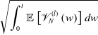 $\sqrt {\displaystyle \int _{0}^{t} \mathbb{E} \left [\mathscr{V}_{N}^{\kern2.6pt(l)}\left ( w \right ) \right ]dw}$
is equivalent to plotting
 $\sigma \left ( {\mathscr{M}^{\kern1.6pt(l)}_{N} \left ( t \right ) }\right )$
for each
 $l$
and
 $N$
.
Output of
 $\sigma ( {\mathscr{M}^{\kern1.6pt(l)}_{N} ( t ) })$
and
 $\sigma ( {\mathfrak{G}^{(l)}_{N} ( t) })$
for
 $l=1,2,3,4,$
and
 $5$
. The dark red, blue, green, purple, teal, orange and black curves correspond to
 $N=550$
,
 $1300$
,
 $2900$
,
 $7000$
,
 $15000$
,
 $30000$
, and
 $60000$
, respectively. All other parameters and initial data are the same as those used to generate Figure 2
.

In each panel, the dark red, blue, green, purple, teal, orange and black curves correspond to
 $N=550$
,
 $1300$
,
 $2900$
,
 $7000$
,
 $15000$
,
 $30000$
and
 $60000$
, respectively, as indicated in the legend of panel (a). All other parameters and initial data are the same as those used to generate Figure 2. The expectations involved in computing these standard deviations are approximated by averaging the outputs of 70 random sample paths of the SIHRS-IPC model for each fixed pair of
 $N$
and
 $l$
.
Additionally, similar to Figure 9, we repeat the computations in Figure 10 using larger ensembles of stochastic sample paths. In particular, Figure 11 recomputes the statistics
 $\sigma \left ( {\mathfrak{G}^{(l)}_{N} \left ( t\right ) }\right )$
shown in panels (f)–(j) of Figure 10. Specifically, Figure 11 is generated using 80 stochastic sample paths for panels (a)–(e) and 90 stochastic sample paths for panels (f)–(j), while all other parameters, initial data and computational procedures remain unchanged.
Output of
 $\sigma ( {\mathfrak{G}^{(l)}_{N} (t) })$
for
 $l=1,2,3,4,$
and
 $5$
. The dark red, blue, green, purple, teal, orange and black curves correspond to
 $N=550$
,
 $1300$
,
 $2900$
,
 $7000$
,
 $15000$
,
 $30000$
and
 $60000$
, respectively. All parameters and initial data are identical to those used to generate panels (f)–(j) in Figure 10
, except that the numbers of stochastic sample paths are increased to 80 for panels (a)–(e) and 90 for panels (f)–(j).

Figure 11. Long description
The image contains ten line graphs, each depicting statistics related to different variables over time in days. The graphs are organized into two rows, each containing five panels. Panel A shows statistics related to s N(t), Panel B shows statistics related to i N(t), Panel C shows statistics related to h N(t), Panel D shows statistics related to r N(t), and Panel E shows statistics related to d N(t). The second row repeats the same variables in Panels F to J. Each graph has the x-axis labeled as Time (days) and the y-axis labeled as sigma (with different subscripts and variables). The dark red, blue, green, purple, teal, orange, and black curves correspond to different parameters. All parameters and initial data are identical to those used to generate panels (f)-(j) in Figure 10, except that the numbers of stochastic sample paths are increased to 80 for panels (a)-(e) and 90 for panels (f)-(j). The graphs show various trends and patterns over a period of 1000 days, with each curve representing different expectations and variances.
The plots in Figure 10 provide evidence of finite-size effects for both
 $\sigma \left ( {\mathfrak{G}^{(l)}_{N} \left ( t \right ) }\right )$
and
 $ \sigma \left ( {\mathscr{M}^{\kern1.6pt(l)}_{N} \left ( t \right ) }\right )$
. As with the other finite-size statistics presented in Figure 8, both quantities in Figure 10 show a general trend of increasing as the population size
 $N$
decreases. Noticeable exceptions mainly occur for
 $ \sigma \left ( {\mathscr{M}^{\kern1.6pt(l)}_{N} \left ( t \right ) } \right )$
for the two smallest population sizes,
 $N=550$
and
 $N=1300$
, during the late stage of the epidemic (see, for example, the corresponding curves in panel (f) of Figure 10). As explained in Section 4.2 and further illustrated by the early-die-out diagnostics in panels (f)–(j) of Figure 8, these deviations stem from the increased prevalence of early-die-out trajectories in the smallest populations; they can alter the late-time ordering of the curves.
Furthermore, the results shown in Figure 11, obtained using 80 random paths for panels (a)–(e) and 90 random paths for panels (f)–(j), instead of the 70 stochastic sample paths used in Figure 10, exhibit essentially the same ordering of the curves and the same overall finite-size trends. In particular, the same late-time exceptions for the smallest population sizes persist after increasing the numbers of stochastic sample paths. This lends further evidence that the observed exceptions are more likely to reflect the intrinsic stochastic dynamics associated with the prevalence of early-die-out trajectories than to be artefacts of estimating the sample averages from only 70 sample paths.
To explain these observations, we begin with an analysis of
 $\sigma \left ( \mathscr{M}^{\kern1.6pt(l)}_{N} \left ( t \right ) \right )$
for small values of
 $t$
. We further analyse
 $\sigma \left ( {\mathfrak{G}^{(l)}_{N} \left ( t \right ) }\right )$
and demonstrate that it admits an upper bound that scales like
 $1/\sqrt {N}$
for early times, which provides a theoretical explanation for the finite-size effects observed in the behaviour displayed in panels (f)–(j) of Figure 10.
6.2. An early-time analysis of
$\sigma ({{\mathscr{M}}^{(l)}_{N}} (t))$

Using Eq. (3.3) and the additivity of the variance in time for martingales, for sufficiently small
 $\Delta t$
, we have
 \begin{equation} {\operatorname {Var}} \left ( {\mathscr{M}^{\kern1.6pt(l)}_{N} \left (k \Delta t \right ) } \right )=\sum \limits _{j = 0 }^ {k-1} {\operatorname {Var}} \left ( { \Delta \mathscr{M}^{\kern1.6pt(l)}_{N} (j\Delta t) }\right )\!, \end{equation}
where
 $ { \Delta \mathscr{M}^{\kern1.6pt(l)}_{N} (t)} = { \mathscr{M}^{\kern1.6pt(l)}_{N} (t+\Delta t) }- { \mathscr{M}^{\kern1.6pt(l)}_{N} (t)}$
. Thus, to estimate
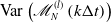 ${\operatorname {Var}} \left ( {\mathscr{M}^{\kern1.6pt(l)}_{N} \left (k \Delta t \right ) } \right )$
, it suffices to estimate
 ${\operatorname {Var}} \left ( \Delta \mathscr{M}^{\kern1.6pt(l)}_{N} (j\Delta t) \right )$
for
 $j \leq k-1$
.
 \begin{equation} {\operatorname {Var}} \left ( \Delta \mathscr{M}^{\kern1.6pt(l)}_{N} (j\Delta t) \right ) = \int _ {j \Delta t } ^ {(j+1)\Delta t} \mathbb{E}\left [\mathscr{V}_{N}^{\kern2.6pt(l)} (w) \right ] dw \approx \Delta t \mathbb{E}\left [\mathscr{V}_{N}^{\kern2.6pt(l)} (j\Delta t) \right ] , \quad l = 1, 2, 3, 4, 5. \end{equation}
Subsequently, we estimate
 $ \mathbb{E}\left [\mathscr{V}_{N}^{\kern2.6pt(l)} (j\Delta t) \right ]$
by taking
 $j=0,1$
for
 $l=1,2,3,4,5$
and additionally
 $j=2$
for
 $l=3,4,5$
.
6.2.1. An early-time-step estimation
First, taking
 $j=0$
in Eq. (6.6), from Eq. (3.4), we infer
 \begin{equation} \mathbb{E}\left [\mathscr{V}_{N}^{\kern2.6pt(l)} (0) \right ] = \mathbb{E}\left [\mathscr{V}_{N}^{\kern2.6pt(l)} (\overrightarrow { {m}_{0 }} ) \right ]\cong \dfrac {1}{N},\quad l = 1, 2, 3, 4, 5, \end{equation}
Next, taking
 $j=1$
in Eq. (6.6) and considering
 $l=1$
, from Eqs. (3.4)
 $_1$
Eq. (A.25), we infer that
 \begin{equation} \begin{aligned} \mathbb E \left [ \mathscr{V}^{\kern1.8pt(1)}_{N} \left ( \Delta t \right ) \right ] & = \dfrac {1}{N}\left ( \beta _{SI} \mathbb E \left [ \textbf s_N(\Delta t) \textbf i_N(\Delta t) \right ] + \lambda _{RS} \mathbb E \left [\textbf r_N(\Delta t) \right ] \right ) \\ & \approx \dfrac {1}{N}\left ( \beta _{SI} \left (s ( \Delta t) i ( \Delta t) -\dfrac {1}{N} \beta _{SI} s_{0N} i_{0N}\Delta t \right ) + \lambda _{RS} r (\Delta t)\right ) \\ &= \dfrac {1}{N}\left ( -\dfrac {\left (\beta _{SI} \right )^2}{N} s_{0N} i_{0N} \Delta t +\beta _{SI} s (\Delta t) i (\Delta t) + \lambda _{RS} r (\Delta t) \right )\!. \end{aligned} \end{equation}
With a similar computation, we obtain a parallel estimate for
 $l=2$
:
 \begin{equation} \begin{aligned} \mathbb E \left [ \mathscr{V}^{\kern1.8pt(2)}_{N} \left ( \Delta t \right ) \right ] &= \dfrac {1}{N}\left ( ( \gamma _{IH}+\gamma _{IR}+\gamma _{ID}) \mathbb E \left [ \textbf i_N(\Delta t) \right ] + \beta _{SI} \mathbb E \left [\textbf s_N(\Delta t) \textbf i_N(\Delta t) \right ] \right ) \\ &=\dfrac {1}{N}\left (-\dfrac { \beta _{SI} ^2}{N} s_{0N} i_{0N} \Delta t + ( \gamma _{IH}+\gamma _{IR}+\gamma _{ID}) i (\Delta t) + \beta _{SI} {s }(\Delta t) {i}(\Delta t) \right )\!. \end{aligned} \end{equation}
This, together with Eq. (6.8), implies that
 \begin{equation} \begin{aligned} \mathbb E \left [ \mathscr{V}^{\kern1.8pt(l)}_{N} \left ( \Delta t \right ) \right ] \cong \dfrac {1}{N}, \quad l = 1, 2, \end{aligned} \end{equation}
where we have discarded lower-order terms of magnitude
 $ {O} \left (\dfrac {\Delta t}{N^{2}}\right )$
on the right-hand sides of Eqs. (6.8) and (6.9).
For
 $l=3,4,5$
, using the linearity of expectation together with Eq. (5.8) and Eq. (3.4)
 $_3$
, Eq. (3.4)
 $_4$
and Eq. (3.4)
 $_5$
, we have
 \begin{equation} \mathbb E \left [ \mathscr{V}^{\kern1.8pt(l)}_{N} \left ( \overrightarrow {\textbf {m}_N( \Delta t)} \right ) \right ] = \mathscr{V}^{\kern1.8pt(l)}_{N} \left (\mathbb E \left [ \left ( \overrightarrow {\textbf {m}_N( \Delta t)}\right ) \right ] \right ) = \mathscr{V}^{\kern1.8pt(l)}_{N} \left ( \overrightarrow { {m} ( \Delta t)} \right ) \cong \dfrac {1}{N} , \quad l = 3, 4, 5. \end{equation}
This, together with (6.10), implies that
 \begin{equation} \begin{aligned} \mathbb E \left [ \mathscr{V}^{\kern1.8pt(l)}_{N} \left ( \Delta t \right ) \right ] \cong \dfrac {1}{N}, \quad l = 1, 2, 3, 4, 5. \end{aligned} \end{equation}
Finally, taking
 $j=2$
in (6.6), we analyse cases
 $l=3,4,5$
. From the linearity of expectation, together with Eq. (3.4)
 $_3$
, Eq. (3.4)
 $_4$
, Eq. (3.4)
 $_5$
and Eq. (5.13), we have
 \begin{equation} \mathbb E \left [ \mathscr{V}^{\kern1.8pt(l)}_{N} \left ( \overrightarrow {\textbf {m}_N( 2\Delta t)} \right ) \right ] = \mathscr{V}^{\kern1.8pt(l)}_{N} \left (\mathbb E \left [ \left ( \overrightarrow {\textbf {m}_N(2 \Delta t)}\right ) \right ] \right ) \approx \mathscr{V}^{\kern1.8pt(l)}_{N} \left ( \overrightarrow { {m} ( 2\Delta t)} \right ) \cong \dfrac {1}{N} , \quad l = 3, 4, 5. \end{equation}
6.2.2. Explanations for the finite-size effects
From Eqs. (6.12), (6.13), (6.7), and (6.5), we infer that
 \begin{equation} \begin{aligned} \begin{cases} \sigma \left ( { \mathscr{M}^{\kern1.6pt(l)}_{N} (k\Delta t ) } \right )\cong \sqrt {\dfrac {\Delta t}{N}}, \quad k = 1, 2, \quad l = 1, 2, 3, 4, 5, \\[10pt] \sigma \left ( { \mathscr{M}^{\kern1.6pt(l)}_{N} (3\Delta t ) } \right ) \cong \sqrt {\dfrac {\Delta t}{N}}, \quad l = 3, 4, 5. \end{cases} \end{aligned} \end{equation}
From Eq. (6.14) we infer that, at least for sufficiently small times, martingale fluctuations exhibit a clear finite-size ordering. Specifically, for
 $ 0\lt N \lt \tilde {{ N}}$
, we have
 \begin{equation} \begin{aligned} \begin{cases} \sigma \left ( { \mathscr{M}^{\kern1.6pt(l)}_{N} (k\Delta t ) } \right ) \gt \sigma \left ( { \mathscr{M}^{\kern1.6pt(l)}_{ \tilde N} (k\Delta t ) } \right )\!, \quad k = 1, 2, \quad l = 1, 2, 3, 4, 5, \\[2pt] \sigma \left ( { \mathscr{M}^{\kern1.6pt(l)}_{N} (3\Delta t ) } \right ) \gt \sigma \left ( { \mathscr{M}^{\kern1.6pt(l)}_{ \tilde N} (3\Delta t ) } \right )\!, \quad l = 3, 4, 5. \end{cases} \end{aligned} \end{equation}
This indicates that smaller population sizes lead to larger stochastic fluctuations in the martingale component during early-time evolution. Motivated by this observation, we conjecture that the ordering in Eq. (6.15) persists beyond the initial few time steps. More precisely, we conjecture that for
 $ 0\lt N \lt \tilde N$
,
 \begin{equation} \begin{aligned} \sigma \left ( { \mathscr{M}^{\kern1.6pt(l)}_{N} ( t ) } \right ) \gt \sigma \left ( { \mathscr{M}^{\kern1.6pt(l)}_{ \tilde N} ( t ) } \right )\! , \quad t \in \left[0, \tau ^{(l)}_{N}\right]\!, \quad l = 1, 2, 3, 4, 5, \end{aligned} \end{equation}
where
 $\tau ^{(l)}_{N}$
may depend on both the compartment index
 $l$
and population size
 $N$
. This conjecture provides a theoretical basis for the finite-size effects observed in panels (a)–(e) of Figure 10, where smaller values of
 $N$
consistently produce larger stochastic fluctuations in the martingale component.
6.3. An early-time analysis of
$\sigma ({\mathfrak{G}}^{(l)}_{N} (t))$

We now explain the finite-size effects observed for
 $ \sigma \left ( \mathfrak{G}^{(l)}_{N} \left ( t\right ) \right )$
. Our goal is to show that, at least for sufficiently small times
 $t$
, this quantity admits an upper bound that decreases as the population size
 $N$
increases.
Taking
 $t =k \Delta t$
and computing the variance on both sides of Eq. (6.1) and then applying the Cauchy–Schwarz inequality, we obtain
 \begin{equation} \begin{aligned} {\operatorname {Var}} \left ( \mathfrak{G}_{N}^{(l)}(k\Delta t) \right ) & = {\operatorname {Var}} \left ( \sum \limits _{j = 0}^ k \Delta \mathfrak{G}_{N}^{(l)}(j\Delta t) \right ) \\ & = \sum \limits _{j = 0}^ k {\operatorname {Var}} \left ( \Delta \mathfrak{G}_{N}^{(l)}\left ( j \Delta t \right ) \right ) + 2 \sum \limits _{j_1 \lt j_2} {\operatorname {Cov}} \left ( \Delta \mathfrak{G}_{N}^{(l)} \left ( j_1 \Delta t \right )\!, \Delta \mathfrak{G}_{N}^{(l)}\left ( j_2 \Delta t \right ) \right ) \\ &\leq k \sum \limits _{j = 0}^ k {\operatorname {Var}} \left ( \Delta \mathfrak{G}_{N}^{(l)}\left ( j \Delta t \right ) \right )\!, \quad l = 1, 2, 3,4, 5, \end{aligned} \end{equation}
where
 $ \Delta \mathfrak{G}_{N}^{(l)}( t)$
denotes the increment
 $ \mathfrak{G}^{(l)}_{N} (t+\Delta t) - \mathfrak{G}^{(l)}_{N} (t)$
. Therefore, to bound
 ${\operatorname {Var}} \left ( \mathfrak{G}_{N}^{(l)}(k\Delta t) \right )$
, it suffices to bound
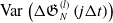 ${\operatorname {Var}} \left ( \Delta \mathfrak{G}_{N}^{(l)}\left ( j \Delta t \right ) \right )$
for
 $j \leq k$
. For sufficiently small
 $\Delta t$
, we have
 \begin{equation} {\operatorname {Var}} \left ( \Delta \mathfrak{G}_{N}^{(l)}\left ( j \Delta t \right ) \right ) = {\operatorname {Var}} \left (\int _{j \Delta t} ^ {(j+1) \Delta t} {\mathscr{G}^{\kern1pt(l)}_{N} \left ( w \right ) } dw \right ) \approx \left (\Delta t \right ) ^2 {\operatorname {Var}} \left ( \mathscr{G}^{\kern1pt(l)}_{N} \left ( j \Delta t \right )\right )\!. \end{equation}
Subsequently, we will estimate
 ${\operatorname {Var}} \left ( \mathscr{G}^{\kern1pt(l)}_{N} \left ( j \Delta t \right )\right )$
by considering the cases
 $j=0$
and
 $j=1$
.
6.3.1. A first and second time step analysis of
${\operatorname {Var}}\, ( \mathscr{G}^{\kern1pt(l)}_{N} (t))$

We begin with the first time step. Taking
 $ j= 0$
in Eq. (6.18), we obtain
 \begin{equation} \begin{aligned} {\operatorname {Var}} \left ( \Delta \mathfrak{G}_{N}^{(l)}\left ( 0 \right ) \right ) = {\operatorname {Var}} \left ( \mathscr{G}^{\kern1pt(l)}_{N} \left ( 0\right ) \right ) = {\operatorname {Var}} \left ({\mathscr{G}^{\kern1pt(l)} (\overrightarrow { {m}_{0 }} ) } \right ) = 0 , \quad l = 1, 2, 3, 4, 5. \end{aligned} \end{equation}
This follows from the fact that the initial condition
 $\overrightarrow { {m}_{0 }}$
is deterministic, as specified in Eq. (4.5). Combining Eq. (6.19) with Eq. (6.4), we infer that at the first time step,
 \begin{equation} \begin{aligned} \sigma \left ({ {\textbf {m}^{(l)}_{N}(\Delta t) }}\right ) & \approx \sigma \left ( { \mathscr{M}^{\kern1.6pt(l)}_{N} (\Delta t ) }\right )\!, \quad l =1, 2, 3, 4, 5 . \end{aligned} \end{equation}
Thus, at this early stage, the standard deviation of each compartment is dominated by the martingale component, whereas the contribution from the infinitesimal mean term is negligible.
Next, taking
 $j=1$
in Eq. (6.18), for
 $l=1$
, and using Eq. (3.2), we obtain
 \begin{equation} \begin{aligned} {\operatorname {Var}}\left ( \mathscr{G}^{\kern1pt(1)}_{N} (\Delta t) \right ) & = \beta _{SI} ^2{\operatorname {Var}}\left ( \textbf s_N( \Delta t) \textbf i_N( \Delta t) \right ) + \lambda _{RS} ^2 {\operatorname {Var}} \left (\textbf r_N(\Delta t) \right ) \\ &\quad - {2} \beta _{SI} \lambda _{RS} {\operatorname {Cov}} \left ( \textbf s_N( \Delta t) \textbf i_N( \Delta t) , \textbf r_N( \Delta t) \right )\!. \end{aligned} \end{equation}
Applying the Cauchy–Schwarz inequality to the covariance term on the right-hand side yields
 \begin{equation*} \left | {\operatorname {Cov}} \left ( \textbf s_N( \Delta t) \textbf i_N( \Delta t) , \textbf r_N( \Delta t) \right ) \right | \leq \sqrt {{\operatorname {Var}}\left ( \textbf s_N( \Delta t) \textbf i_N( \Delta t) \right ) }\sqrt { {\operatorname {Var}} \left (\textbf r_N(\Delta t) \right )} . \end{equation*}
Combining this bound with Eqs. (6.21), (6.6), (3.4), and (A.20), we obtain
 \begin{equation} \begin{aligned} {\operatorname {Var}}\left ( \mathscr{G}^{\kern1pt(1)}_{N} (\Delta t) \right ) &\leq 2 \beta _{SI} ^2 {\operatorname {Var}}\left ( \textbf s_N( \Delta t) \textbf i_N( \Delta t) \right ) +2 \lambda _{RS} ^2 {\operatorname {Var}} \left (\textbf r_N(\Delta t) \right ) \\ &\approx 2 \beta _{SI} ^2 {\mathbb{E}\left [\mathscr{W}_{N} \left ( \overrightarrow { {m}_{0 }} \right ) \right ]\Delta t} +2 \lambda _{RS} ^2 {\operatorname {Var}} \left ( { \mathscr{M}^{\kern1.6pt(4)}_{N} (\Delta t ) } \right ) \\ &\approx 2\Delta t\left ( \beta _{SI} ^2 \mathbb{E}\left [\mathscr{W}_{N} (\overrightarrow { {m}_{0 }} ) \right ] + \lambda _{RS} ^2 \mathbb{E}\left [\mathscr{V}_{N}^{\kern2.6pt(4)} (\overrightarrow { {m}_{0 }} ) \right ] \right )\!. \end{aligned} \end{equation}
With a similar computation, we obtain a parallel estimate for the case
 $l=2$
:
 \begin{equation} \begin{aligned} {\operatorname {Var}}\left ( \mathscr{G}^{\kern1pt(2)}_{N} (\Delta t) \right ) &\leq 2\beta _{SI} ^2 {\operatorname {Var}}\left ( \textbf i_N( \Delta t) \textbf s_N( \Delta t) \right ) + 2\left ( \gamma _{IH} + \gamma _{IR} + \gamma _{ID} \right )^2 {\operatorname {Var}} \left (\textbf i_N( \Delta t) \right ) \\ &\approx 2 \Delta t \left ( \beta _{SI} ^2 \mathbb{E}\left [\mathscr{W}_{N} (\overrightarrow { {m}_{0 }} ) \right ] +2 \left ( \gamma _{IH} + \gamma _{IR} + \gamma _{ID} \right )^2 \mathbb{E}\left [\mathscr{V}_{N}^{\kern2.6pt(2)} (\overrightarrow { {m}_{0 }} ) \right ] \right )\!. \end{aligned} \end{equation}
Together with Eqs. (6.22) and (A.15), this implies
 \begin{equation} {\operatorname {Var}} \left ({\mathscr{G}^{\kern1pt(l)}_{N} (\Delta t) } \right ) \lesssim \dfrac { \Delta t }{N}, \quad l = 1, 2, \end{equation}
where
 $\lesssim$
denotes an inequality up to a positive multiplicative constant depending only on the initial data and model parameters and independent of
 $N$
.
Finally, we deal with cases
 $l = 3, 4, 5$
. Using the Cauchy–Schwarz inequality together with Eq. (6.6), Eq. (3.2)
 $_3$
, Eq. (3.4)
 $_3$
and Eq. (6.20), we obtain the following estimate for
 $l=3$
:
 \begin{equation} \begin{aligned} {\operatorname {Var}}\left ( \mathscr{G}^{\kern1pt(3)}_{N} (\Delta t) \right ) & \leq 2 \gamma _{IH} ^2{\operatorname {Var}}\left ( \textbf i_N( \Delta t) \right ) +2 \left ( \alpha _{HR} + \alpha _{HD} \right )^2 {\operatorname {Var}} \left (\textbf h_N(\Delta t ) \right ) \\ & \approx 2 \gamma _{IH} ^2 {\operatorname {Var}}\left ( { \mathscr{M}^{\kern1.6pt(2)}_{N} (\Delta t ) } \right ) +2 \left ( \alpha _{HR} + \alpha _{HD} \right )^2 {\operatorname {Var}} \left ( { \mathscr{M}^{\kern1.6pt(3)}_{N} (\Delta t ) } \right ) \\ & \approx 2\Delta t \gamma _{IH} ^2 \mathbb{E}\left [\mathscr{V}_{N}^{\kern2.6pt(2)} (\overrightarrow { {m}_{0 }} ) \right ] +2\Delta t \left ( \alpha _{HR} + \alpha _{HD} \right )^2 \mathbb{E}\left [\mathscr{V}_{N}^{\kern2.6pt(3)} (\overrightarrow { {m}_{0 }} ) \right ]\! . \end{aligned} \end{equation}
With similar computations, for
 $l = 4, 5$
, we obtain
 \begin{equation*} \begin{aligned} \begin{cases} {\operatorname {Var}}\left ( \mathscr{G}^{\kern1pt(4)}_{N} (\Delta t) \right ) &\!\!\!\!\leq 3 \left ( \beta _{SI} ^2{\operatorname {Var}}\left ( \textbf i_N( \Delta t) \right ) + \alpha _{HR} ^2 {\operatorname {Var}} \left (\textbf h_N( \Delta t) \right ) + \lambda _{RS} ^2 {\operatorname {Var}} \left (\textbf r_N(\Delta t) \right ) \right )\!, \\ &\!\!\!\!\approx 3\Delta t \left ( \beta _{SI} ^2 \mathbb{E}\left [\mathscr{V}_{N}^{\kern2.6pt(2)} (\overrightarrow { {m}_{0 }} ) \right ] + \alpha _{HR} ^2 \mathbb{E}\left [\mathscr{V}_{N}^{\kern2.6pt(3)} (\overrightarrow { {m}_{0 }} ) \right ] + \lambda _{RS} ^2 \mathbb{E}\left [\mathscr{V}_{N}^{\kern2.6pt(4)} (\overrightarrow { {m}_{0 }} ) \right ] \right )\!, \\ {\operatorname {Var}}\left ( \mathscr{G}^{\kern1pt(5)}_{N} (\Delta t) \right ) &\!\!\!\!\leq 2 \left ( \gamma _{ID} ^2{\operatorname {Var}}\left ( \textbf i_N( \Delta t) \right ) + \alpha _{HD} ^2 {\operatorname {Var}} \left (\textbf h_N( \Delta t) \right ) \right ) \\ &\!\!\!\!\approx 2\Delta t \left ( \gamma _{ID} ^2 \mathbb{E}\left [\mathscr{V}_{N}^{\kern2.6pt(2)} (\overrightarrow { {m}_{0 }} ) \right ] + \alpha _{HD} ^2 \mathbb{E}\left [\mathscr{V}_{N}^{\kern2.6pt(3)} (\overrightarrow { {m}_{0 }} ) \right ] \right )\!. \\ \end{cases} \end{aligned} \end{equation*}
This, together with Eq. (6.25), Eq. (3.4)
 $_3$
, Eq. (3.4)
 $_4$
and Eq. (3.4)
 $_5$
, implies that
 \begin{equation} {\operatorname {Var}} \left ({\mathscr{G}^{\kern1pt(l)}_{N} (\Delta t) } \right ) \lesssim \dfrac { \Delta t }{N}, \quad l = 3, 4, 5. \end{equation}
6.3.2. An explanation of the finite-size effects for
$ \sigma ({\mathfrak{G}}_{N}^{(l)}(t))$

Using the estimates of
 $ {\operatorname {Var}} \left ( \mathscr{G}^{\kern1pt(l)}_{N} \left ( j \Delta t \right )\right )$
for
 $ j = 0$
and
 $j=1$
established, we are now ready to estimate
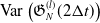 ${\operatorname {Var}} \left ( \mathfrak{G}_{N}^{(l)}(2\Delta t) \right )$
. From Eqs. (6.26), (6.24), (6.19), and (6.17), we infer that
 \begin{equation} \begin{aligned} \sigma \left ( \mathfrak{G}_{N}^{(l)}(2\Delta t) \right ) &\leq 2 \sum \limits _{j = 0}^ 2 {\operatorname {Var}} \left ( \Delta \mathfrak{G}_{N}^{(l)}\left ( j \Delta t \right ) \right ) \\ &\approx 2 \left (\Delta t \right ) ^2 \left ({\operatorname {Var}} \left ( \mathscr{G}^{\kern1pt(l)}_{N} \left ( 0\right )\right ) + {\operatorname {Var}} \left ( \mathscr{G}^{\kern1pt(l)}_{N} \left ( \Delta t \right )\right ) \right ) \\ & \lesssim \Delta t \sqrt {\dfrac { \Delta t }{N}} , \quad l = 1, 2, 3, 4, 5. \end{aligned} \end{equation}
This implies that, at least over the early time steps, the upper bound of
 $\sigma \left ( \mathfrak{G}_{N}^{(l)}(2\Delta t) \right )$
is a decreasing function of population size
 $N$
. We conjecture that this scaling behaviour persists up to a later time
 $ T^{(l)}_{N}$
, for
 $l = 1, 2, 3, 4, 5$
, where
 $T^{(l)}_{N}$
may depend on
 $ l$
for a fixed
 $N$
. This conjecture offers a theoretical explanation for the finite-size effects observed in the evolution of
 $\sigma \left ( \mathfrak{G}_{N}^{(l)}(2\Delta t) \right )$
as illustrated in panels (f)–(j) of Figure 10.
7. Finite-size effects in a case study
To complement the numerical investigations in the preceding sections, we present in this section, a case study based on data from a single real-world community, rather than relying on parameters estimated from national-level COVID-19 data (Section 2.3.1). Specifically, we use epidemiological data from the COVID-19 outbreak in Carson City, Nevada, covering the period from March 25, 2020 to December 5, 2021. The calibration is performed using reported daily confirmed cases and hospitalization data from publicly available sources, including The New York Times COVID-19 data repository [60]. The simulation results are shown in Figure 12.
Output of the I and H compartment fractions with parameters and initial data drawn from the COVID-19 trajectory in Carson City, Nevada, from March 25, 2020 to December 5, 2021. In particular, for simulations of the SIHRS-IPC model, the total population size is set to
 $N = 58,639$
. All other parameter values are listed in Table 5
. Panel (a) displays 20 random paths of
 $\mathbf {i}_N (t)$
(shown in pink), together with the curve of daily confirmed cases (light green), while Panel (c) shows the corresponding
 $90\%$
envelope (pink shaded region), along with the deterministic solution
 $i(t)$
(dark brown dashed line) and the curve of daily confirmed cases (light green). Panel (b) displays 30 random paths of
 $\mathbf {h}_N (t)$
(dark green), together with the curve of daily confirmed hospitalizations (magenta). Panel (d) shows the corresponding
 $90\%$
envelope (dark green shaded region), along with the deterministic solution
 $h(t)$
(purple dashed line) and the curve of daily confirmed hospitalizations (magenta). Moreover, panels (e) and (f) show the path averages of
 $\mathbf {i}_N (t)$
(blue) and
 $\mathbf {h}_N (t)$
(black), respectively, together with the corresponding observed data and deterministic solutions.

Figure 12. Long description
The image contains six panels of line graphs depicting the output of the I and H compartment fractions with parameters and initial data drawn from the COVID-19 trajectory in Carson City, Nevada, from March 25, 2020 to December 5, 2021. Panel A: A line graph showing 20 random paths of i_N(t) in pink, together with the curve of daily confirmed cases in light green. The x-axis represents the date from March 25, 2020, to December 5, 2021, and the y-axis represents the infected compartment fraction. Panel B: A line graph displaying 30 random paths of h_N(t) in dark green, together with the curve of daily confirmed hospitalizations in magenta. The x-axis represents the date from March 25, 2020, to December 5, 2021, and the y-axis represents the hospitalized compartment fraction. Panel C: A line graph showing the 90% envelope of i_N(t) in pink shaded region, along with the deterministic solution in dark brown dashed line and the curve of daily confirmed cases in light green. The x-axis represents the date from March 25, 2020, to December 5, 2021, and the y-axis represents the infected compartment fraction. Panel D: A line graph showing the 90% envelope of h_N(t) in dark green shaded region, along with the deterministic solution in purple dashed line and the curve of daily confirmed hospitalizations in magenta. The x-axis represents the date from March 25, 2020, to December 5, 2021, and the y-axis represents the hospitalized compartment fraction. Panel E: A line graph showing the path average of i_N(t) in blue, together with the corresponding observed data in light green and the deterministic solution in dark brown dashed line. The x-axis represents the date from March 25, 2020, to December 5, 2021, and the y-axis represents the infected compartment fraction. Panel F: A line graph showing the path average of h_N(t) in black, together with the corresponding observed data in magenta and the deterministic solution in purple dashed line. The x-axis represents the date from March 25, 2020, to December 5, 2021, and the y-axis represents the hospitalized compartment fraction.
The purpose of this case study is not to provide a precise epidemiological forecast, but rather to illustrate how the finite-size effects identified in earlier sections can manifest in practice within a realistic population setting, using empirically grounded parameters and initial conditions. In comparison with ensembles of agent-based SIHRS-IPC simulations, the corresponding deterministic model fails to reproduce several key dynamical features, including early die-out events, pronounced variability across stochastic realizations and persistent irregular fluctuations over time. These behaviours are consistent with, and anticipated by, the finite-size analysis developed in this study.
7.1. Parameter and initial data choices
To generate simulations of the SIHRS-IPC model, the total population size is fixed at the actual census value for Carson City, Nevada, namely
 $N = 58{,}639$
, based on the 2020 U.S. Census. The initial conditions for the infected and deceased compartments,
 $i_0$
and
 $d_0$
, are chosen directly from the data reported on March 25, 2020. Specifically, we set
 $i_0=3/58{,}639$
and
 $d_0 =0$
. We set the initial hospitalized and recovered populations to zero, that is,
 $h_0 = r_0 = 0$
, and determine the initial susceptible fraction as
 $s_0 = 1- \left (i_0 +h_0 + r_0 + d_0 \right )$
. This choice of the initial state reflects the onset of the epidemic (such as the early stage of the COVID-19 outbreak), in which only a small number of infectious individuals had been identified, while no individuals had yet progressed to hospitalization or recovery and consequently no epidemic-induced deaths had yet occurred.
The model parameters are chosen as a combination of those used in Table 3.3.1 and those estimated directly from data specific to Carson City, as summarized in Table 5.
Model parameter values used in simulations for Carson City, Nevada

Table 5. Long description
A table titled `Model parameter values used in simulations for Carson City, Nevada' presents the parameters and their corresponding values. The table has two columns: Parameters and Values. The Parameters column lists the following: beta subscript SI, gamma subscript IH, gamma subscript HR, gamma subscript ID, alpha subscript HR, alpha subscript HD, and lambda subscript RS. The Values column lists the following: 0.157114286, 0.01314285714, 0.1154285714, 0, 0.094, 0.01711, and 0.008134.
The difference between Tables 4 and 5 lies in the values of
 $\beta _{SI}$
,
 $\gamma _{IH}$
and
 $\gamma _{IR}$
; all other parameters, including
 $\alpha _{HR}$
,
 $\alpha _{HD}$
and
 $\lambda _{RS}$
, remain unchanged.
Regarding the choice of
 $\gamma _{IH}$
,
 $\gamma _{IR}$
and
 $\gamma _{ID}$
, Table 2 indicates that it suffices to estimate the quantities
 $\gamma$
,
 $p_{IH}$
,
 $p_{IR}$
and
 $p_{ID}$
. We continue to use the same values of
 $\gamma$
and
 $p_{ID}$
as described in Section 2.3.1. For
 $p_{IH}$
, however, we compute it directly from Carson City data as the 7-day moving average of the ratio between hospitalized patients and active cases (see, e.g., [Reference Arita6, Reference Bergman, Sella, Agre and Casadevall8, Reference Bhowmik, Tirtha, Iraganaboina, Eluru and Liu12] for discussions of moving-average techniques). Using the confirmed case and hospitalization data from [60], we obtain
 $p_{IH}=0.092$
.
We suspect that this value of
 $p_{IH}$
is slightly higher than that used in Section 2.3.1, partly because of a low ascertainment rate of COVID-19 infections in the United States (see, e.g., [Reference Clarke, Jones, Deng, Nycz, Lee, Iachan, Gundlapalli, Hall and MacNeil23, Reference Deng, Kim, Bratcher, Jones, Simuzingili, Gundlapalli, Hagen, Iachan and Clarke24, Reference Reese, Iuliano, Patel, Garg, Kim, Silk, Hall, Fry and Reed55]). In particular, CDC serosurveys indicate that true infection counts exceeded reported case counts by factors of 6–24 during the early phases of the pandemic [Reference Havers, Reed, Lim, Montgomery, Klena, Hall, Fry, Cannon, Chiang, Gibbons, Krapiunaya, Morales-Betoulle, Roguski, Rasheed, Freeman, Lester, Mills, Carroll, Owen and Thornburg34]. Consequently, infectious cases are substantially underreported relative to hospitalizations, leading to a larger empirical estimate of
 $p_{IH}$
when computed directly from the reported data. With
 $p_{IH}$
determined, we obtain
 $p_{IR} = 1- p_{IH} - p_{ID}-p_{II} = 0.8080$
. This yields the updated values
 $\gamma _{IH}=0.01314285714$
and
 $\gamma _{IR}=0.11542857142$
.
For the transmission rate
 $\beta _{SI}$
, Eq. (2.4) shows that it suffices to determine an appropriate basic reproduction number R
 $_0$
for Carson City. We adopt the reported value R
 $_0 = 1.222$
from [Reference Sy, White and Nichols58], which leads to
 $\beta _{SI}$
=R
 $_0$
 $\left ( \gamma _{IH} + \gamma _{IR} + \gamma _{ID} \right ) = 0.15711428571$
.
7.2. Simulation output
Figure 12 displays the simulation output for the compartment fractions of
 $I$
and
 $H$
, as shown in the first and second rows, respectively. In panel (a), we plot 20 random sample paths of
 $\textbf {i}_N(t)$
(shown in pink), together with the curve of daily confirmed cases (shown in light green). Panel (b) presents the corresponding
 $90\%$
envelope, defined by the 5th and 95th percentiles across the 20 stochastic simulations (pink shaded region), along with the deterministic solution
 $i(t)$
(dark brown dashed curve) and daily confirmed case data. Panels (c) and (d) present analogous results for the hospitalized compartment. In panel (c), we plot 30 random sample paths of
 $\textbf {h}_N(t)$
(dark green), together with the daily hospitalization data (magenta). Panel (d) shows the
 $90\%$
envelope across these simulations (dark green shaded region), deterministic trajectory
 $h(t)$
(purple dashed curve) and daily hospitalization data (magenta).
The long-term dynamics of the real-life infectious compartment exhibit clear multiple epidemic waves (panels (a) and (b) in Figure 12), with at least two major outbreaks visible over the simulated time horizon. Throughout this period, the hospitalized compartment remains significantly smaller in magnitude than the infectious compartment. Consequently, although the overall population of Carson City is relatively large (approximately
 $60,000$
), the stochastic fluctuations in
 $\textbf {h}_N(t)$
are large relative to its typical size (panels (c) and (d) in Figure 12). Furthermore, the
 $90\%$
empirical envelopes constructed from ensembles of stochastic sample paths quantify the range of fluctuations around the mean-field trajectories, rather than serving as pointwise fits to the observed data (panels (b) and (d)). In both panels (b) and (d), the lower edge of the envelope can be close to zero because a non-negligible proportion of stochastic realizations experience low-outbreak or early-die-out trajectories. These realizations contribute near-zero values to the empirical 5th percentile, which determines the lower boundary of the
 $90\%$
envelope. At the same time, other realizations exhibit sustained outbreaks with much larger infectious and hospitalized populations, thereby contributing to the upper boundary of the envelope. As a result, the resulting envelope spans a large portion of the plotting region. This interpretation is further supported by panels (e) and (f), where the average of the 30 stochastic sample paths lies well below the upper boundary of the corresponding
 $90\%$
envelope. Moreover, panel (f) shows that, for the comparatively small hospitalized compartment, the average of only 30 stochastic realizations already provides a close approximation to the deterministic ODE trajectory
 $h(t)$
.
The sustained width of these envelopes highlights the persistence of finite-size effects. Consequently, the case study indicates that even when the total population is large, stochastic variability can remain non-negligible in compartments with comparatively small population sizes.
In addition, we emphasize that the comparison among the real-world data, SIHRS-IPC model and SIHRS-ODE model shown in Figure 12 is performed in a fair and internally consistent manner. The observed discrepancies are not the result of artificially degraded parameter choices for the deterministic model, but rather stem from fundamental differences between stochastic epidemic dynamics and their mean-field representations (see Remark 5 for further discussion).
Remark 5. The simultaneous capture of both the timing and magnitude of epidemic peaks and intervening troughs remains a difficult and largely unresolved challenge for standard deterministic ODE-based compartmental models. Periods such as major holidays (e.g., November through January) or the start of the academic year (e.g., September) are often associated with sharp increases in social interactions. These events can create short-lived but intense clustering of individuals in relatively confined and well-mixed environments, leading to sharp transient surges in transmission that are difficult to represent within a fixed-parameter ODE compartmental framework. In addition, during the early phases of the COVID-19 pandemic, widespread limitations in testing availability likely led to a systematic underestimation of the infection counts. This underreporting introduces further discrepancies between the observed data and the model predictions, particularly during low-incidence periods. In light of these factors, we consider the overall agreement between the SIHRS-ODE model and the data (panels (b) and (d) in Figure 12 ) to be reasonable, even though the model reproduces epidemic peaks more faithfully than the intervening troughs.
8. Conclusion and future works
In epidemic modelling, random fluctuations in agent-based formulations with finite population sizes can produce pronounced finite-size effects, leading to systematic departures from mean-field predictions. Consequently, achieving an effective balance between modelling accuracy, computational efficiency and predictive capability necessitates a systematic quantification and careful assessment of the magnitude of finite-size effects. In this study, we investigate finite-size effects in epidemic dynamics using an SIHRS compartmental framework that incorporates immunity waning, thereby naturally allowing for recurrent epidemic waves. In particular, an agent-based SIHRS compartmental model is constructed by assigning Poisson clocks to individual agents to govern the arrival of events (Section 2.1).
By combining numerical simulations with martingale-based early-time asymptotic analysis (Sections 5.1, 6.2 and 6.3), we investigate how finite-size effects vary with population size, compartmental structure and temporal scale. The population sizes
 $N$
explored in our simulations cover a wide spectrum (
 $N=550$
,
 $1300$
,
 $2900$
,
 $7000$
,
 $15000$
,
 $30000$
and
 $60000$
) and are deliberately chosen to be representative of realistic epidemic scenarios, including nursing homes, conferences and social gatherings. Across all parameter regimes examined , the simulation results consistently corroborate the analytical predictions, demonstrating that finite-size effects are not merely theoretical artefacts but can exert a decisive influence on the evolution of epidemic dynamics (see Figures 5, 7, 8, and 10). In particular, the case study (Section 7) focused on a specific U.S. county indicates that even when the total population size is relatively large, stochastic variability can remain significant in key compartments that have a smaller size, most notably the hospitalized compartment (panels (c) and (d) of Figure 12). In summary, our results provide a systematic and quantitative means of identifying the regimes in which mean-field approximations are adequate and those in which agent-based descriptions are necessary to faithfully capture realistic epidemic dynamics, thereby anchoring the proposed theoretical framework in a concrete and interpretable real-world setting.
The results presented here indicate several potential directions for future research. The first direction lies at the interface of the modelling and application. In particular, the explicit inclusion of a hospitalized compartment in the model structure considered here provides a pathway for studying healthcare-related objectives, such as hospital capacity planning, intervention thresholds and risk mitigation under uncertainty. In finite populations, stochastic variability in hospitalization can have significant practical consequences, and incorporating finite-size effects into such analyses may offer more realistic guidance for public health decision-making.
Another natural direction for future work is the further development of the theoretical analysis. In particular, the martingale-based framework can be extended by systematically incorporating higher-order nonlinear terms into the formulation. Systematic analysis of terms involving quadratic, cubic or mixed products of compartment variables has the potential to yield a deeper understanding of how finite-size effects arise from nonlinear coupling between compartments. Such developments could provide sharper theoretical insight into long-time stochastic behaviour that goes beyond the early-time regime examined in the present work.
Furthermore, the modelling framework can be upgraded to incorporate additional epidemiological, behavioural or structural features. These extensions can be achieved, for instance, by incorporating social networks [Reference Abhishek and Srivastava1, Reference Hou, Gao, Li, Kang, Chen, Chen, Rao, Ellenberg and Patz35, Reference Peng, Lu, Lin, Lindstrom, Parkinson, Wang, Bertozzi and Porter53, Reference Ruiz-Herrera and Torres57], agent movement via random walks in two-dimensional space [Reference Xiong, Wang, Zhang and Britton65] and additional compartments representing alerted agents to account for sub-populations adopting preventive behaviours [Reference Bongarti, Galvan, Hatcher, Lindstrom, Parkinson, Wang and Bertozzi14, Reference Guo, Lei, Jiang, Ma, Huo and Zheng32]. Extending the analysis developed in this study to these enriched models would provide valuable insight into how finite-size effects interact with growing model complexity and improved real-life applicability and predictive power.
Acknowledgements
This article is a direct product of the Research Experience for Undergraduates (REU) program in Summer 2025, held by UA Department of Mathematics at The University of Alabama.
Funding statement
Aakash Gurung gratefully acknowledges support from an ASSURE grant from the University of Alabama. Yuanzhen Shao gratefully acknowledges support from NSF grants DMS-2306991 and DMS-2512104.
Competing interests
The authors declare none.
A. Appendix
This appendix contains technical calculations and proofs that are omitted from the main text because of their length and are provided here for completeness.
A.1. Computations of the infinitesimal generators for the SIHRS-IPC model
Infinitesimal generators may be computed using a variety of standard approaches, such as those described in [Reference Applebaum5, Reference Chung and Williams21, Reference Durrett26]. In this section, we adopt a direct approach based on the equivalent description of the SIHRS-IPC model derived in Section 2.2.2. Specifically, we derive the small-time-interval probabilities for the stochastic process
 $\overrightarrow {\textbf {m}_N(t)}$
(e.g., see [Reference Bertsekas and Tsitsiklis11] for a general discussion of small-time-interval probabilities for Poisson-driven processes). These probabilities allow us to compute the corresponding small-time expectations and variances, which form the basis of the infinitesimal generators of the model.
With the new notation
 $\overrightarrow {\Delta \textbf {m}_{N}(t) } \,:\!=\, \overrightarrow {\textbf {m} _{N} (t+\Delta t) }- \overrightarrow {\textbf {m}_{N}(t)}$
, we study the probabilities of small-time increments
 $\overrightarrow {\Delta \textbf {m}_{N}(t) }$
over a short-time interval
 $\Delta t$
, conditioned on the state
 $\overrightarrow { \textbf {m}_{N}(t) }$
at time
 $ t$
. Specifically, we enumerate the possible values of
 $\overrightarrow {\Delta \textbf {m}_{N}(t) }$
and compute their associated probabilities under this condition.
For a sufficiently small
 $\Delta t$
(such that at most one advancement of the sovereign master effective clock occurs), we can compute the conditional probabilities based on the small-time-interval property of a Poisson process (see Remark 6 for details).
As an illustration, consider one possible outcome of
 $ \overrightarrow {\Delta \textbf {m}_{N}(t) }$
, namely
 $(-{1}/N , {1}/{N } , 0, {0}, 0)$
, which corresponds to exactly one susceptible agent transitioning to the infected state. Using Eq. (2.2) together with the second column of Table 3, we obtain
 \begin{equation} \begin{aligned} \mathbb{P}\left ( \overrightarrow {\Delta \textbf {m}_{N}(t) } = \left (- \dfrac {1}{N} , \dfrac {1}{N} ,0,0, 0 \right ) \bigg |\overrightarrow { \textbf {m}_{N}(t) } =\left ( {s} , {i} , {h} , {r} , {d} \right ) \right ) = N { {\beta _{SI}} {i} s\Delta t } + o (\Delta t) , \end{aligned} \end{equation}
where
 $ o (\Delta t)$
denotes a function of
 $\Delta t$
satisfying
 $\lim \limits _{\Delta t \to 0} o (\Delta t) / \Delta t = 0$
, and its precise form may differ at each occurrence.
Among all the possible outcomes of
 $ \overrightarrow {\Delta \textbf {m}_{N}(t) }$
, only two lead to nontrivial changes in
 $\textbf {s}_N ( t)$
, namely,
 $ \left ( {1}/{N},0, - {1}/{N},0 , 0\right )$
and
 $\left ( - {1}/{N}, {1}/{N},0, 0, 0 \right )$
. Thus, by denoting
 $\Delta \textbf {s}(t) =\textbf {s}( t+\Delta t) - \textbf {s}( t)$
, and using the small-time-interval probabilities derived above, we can compute the conditional expectation of
 $\Delta \textbf {s}_N ( t)$
:
 \begin{equation*} \lim \limits _{\Delta t\rightarrow 0}\dfrac {\mathbb E \left [\Delta \textbf {s}_N ( t) \bigg |\overrightarrow { \textbf {m}_{N}(t) } =\left ( {s} , {i} , {h} , {r} , {d} \right ) \right ] }{\Delta t} = \lim \limits _{\Delta t\rightarrow 0} \dfrac { \left ( - { {\beta _{SI}} {i} {s} } + \lambda _{RS}r \right ) \Delta t + o (\Delta t)} {\Delta t} {\color {blue}=} - { {\beta }_{SI} {i} {s} } + \lambda _{RS}r . \end{equation*}
This implies (3.2)
 $_1$
. Using similar computations, we can also obtain the rates of change of the conditional expectations of
 $\Delta \textbf {i}_N ( t)$
,
 $\Delta \textbf {h}_N ( t)$
,
 $\Delta \textbf {r}_N ( t)$
, and
 $\Delta \textbf {d}_{N} (t)$
. These findings provide the corresponding infinitesimal means and consequently yield Eq. (3.2) as desired.
As for the infinitesimal variances, we can again utilize small-interval probabilities. For each
 $l$
, because
 $ \mathscr{V}^{\kern1.8pt( l )}_{N} ( t)$
is the infinitesimal variance of
 $ {\textbf {m}^{(l)}_N(t)}$
, we have
 \begin{align} \mathscr{V}^{\kern1.8pt( l )}_{N} \left( \overrightarrow {\textbf {m}_N(t)} \right) & = \lim _{\Delta t \rightarrow 0} \frac {1}{\Delta t}{\mathbb E \left [ \left ( {\Delta \textbf {m}^{(l)}_{N}(t^ - ) } \right ) ^2 \middle | \overrightarrow {\textbf {m}_N (t^-) } \right ] } , \quad l = 1, 2, 3, 4, 5, \end{align}
where
 $ {\Delta \textbf {m}^{(l)}_{N}(t^ - ) } = \textbf {m}^{(l)}_N (\Delta t+ t^-) - \textbf {m}^{(l)}_N (t^-)$
,
 $l=1, 2, 3, 4, 5$
. As a result, using arguments entirely analogous to those employed for the infinitesimal means above, we can compute the infinitesimal variances from the small-interval probabilities and thereby derive Eq. (3.4).
Remark 6.
In general, for a Poisson process with an arrival rate
 $r$
, the probability of observing
 $k$
arrivals over a time interval of length
 $t$
is given by
 $ e^{-r t}\frac {({r} t)^k}{k!}$
. Taking
 $k=1$
, the probability of a single arrival is therefore
 $e^{-{r} t} {r} t$
. When
 $t$
is sufficiently small, a Taylor expansion of
 $e^{- rt}$
yields
 \begin{equation*} e^{- rt} = 1 - {r} t + \dfrac {{r}^{2} t^{2}}{2} + o (t^2). \end{equation*}
Thus, for a small time interval of length
 $t$
, the probability of exactly one arrival is approximately
 ${r} t$
, up to a higher-order negligible term.
A.2. An upper bound of the martingale variances
As mentioned in Section 3.2, in this section, we derive the upper bounds for the variances of the martingales appearing in the martingale formulations in the spirit of Theorem 3.3 in [Reference Li, Wang, Li and Bertozzi44]. This result implies that the variances of the martingales associated with
 ${\textbf {s}}_{ N}(t)$
,
 ${\textbf {i}}_{ N}(t)$
,
 $ {\textbf {r}}_{ N}(t)$
,
 $ {\textbf {h}}_{ N}(t)$
,
 $ {\textbf {d}}_{ N}(t)$
are bounded in terms of the initial states of each compartment and the total population size
 $N$
. Moreover, these variances are controlled by the quantities of order at most
 $\frac {1}{N}$
. Consequently, as
 $N \rightarrow \infty$
, the stochastic system converges to the corresponding deterministic ODE model.
Theorem 7 (Variance bounds for martingales). The following estimates hold, at least up to the possible blow-up time:
 \begin{equation} \begin{cases} Var\left (\mathscr{M}_{N}^{\kern1.4pt(1)}(t)\right ) \leq \frac {1}{N} \left (\frac {\beta _{SI} }{2}(1 - d_{0N})^{2}t + i_{0N} +h_{0N}+r_{0N}\right )\!, \\[2pt] Var\left (\mathscr{M}_{N}^{\kern1.4pt(2)}(t)\right ) \leq \frac {1}{N} \left ({s_{0N}+h_{0N}+r_{0N}+2\left ( \gamma _{IH} + \gamma _{IR} + \gamma _{ID}\right )(1 - d_{0N})t} \right )\!, \\[2pt] Var\left (\mathscr{M}_{N}^{\kern1.4pt(3)}(t)\right ) \leq \frac {1}{N} \left ( {s_{0N}+i_{0N}+r_{0N}+2\left ( \alpha _{HR} + \alpha _{HD}\right )(1- d_{0N})t}\right )\!, \\[2pt] Var\left (\mathscr{M}_{N}^{\kern1.4pt(4)}(t)\right ) \leq \frac {1}{N}\left ( s_{0N}+i_{0N}+h_{0N} +2\lambda _{RS} (1 - d_{0N})t \right )\!, \\[2pt] Var\left (\mathscr{M}_{N}^{\kern1.4pt(5)}(t)\right ) \leq \frac {1}{N}\left ( 1 - d_{0N} \right )\!. \end{cases} \end{equation}
The proof follows the same strategy as in Theorem 3.3 [Reference Li, Wang, Li and Bertozzi44]. Using Eqs. (3.3) and (3.4), we obtain
 \begin{equation} \begin{aligned} Var\left (\mathscr{M}_{N}^{\kern1.4pt(1)}(t)\right ) &=\frac {1}{N}\left ( 2\beta _{SI} \int _{0}^{t}\mathbb{E}[ \textbf s_N(w) \textbf i_N(w)] dw + \int _{0}^{t}\mathbb{E}\left [\mathscr{G}_{N}^{\kern1.5pt(1)}(w)\right ] dw \right )\!. \end{aligned} \end{equation}
Taking expectations on both sides of the martingale formulation in Eq. (3.1) yields
 \begin{equation} \mathbb{E}[ \textbf s_N(t) ] = s_{0N} + \int _{0}^{t}\mathbb{E}\left [\mathscr{G}_{N}^{\kern1.5pt(1)}(w)\right ]dw . \end{equation}
This together with (A.4) implies
 \begin{equation} Var\left (\mathscr{M}_{N}^{\kern1.4pt(1)}(t)\right ) = \frac {1}{N}\left (2\beta _{SI} \int _{0}^{t}\mathbb{E}[\textbf s_N(w) \textbf i_N(w)]dw + \mathbb{E}[\textbf s_N(t)] - s_{0N}\right )\! . \end{equation}
Note that the maximum possible value of
 $ \textbf s_N(t)$
and
 $ \textbf i_N(t)$
is bounded by
 \begin{equation*} s_{0N} + i_{0N} +h_{0N}+r_{0N} = 1 - d _{0N}. \end{equation*}
Consequently, the product
 $\mathbb{E}[\textbf {s}_N(t)\textbf {i}_N(t)]$
is bounded above by
 $\frac {1}{4}(1-d_{0N})^{2}$
. Therefore, from Eq. (A.6), we deduce that:
 \begin{equation*} Var\left (\mathscr{M}_{N}^{\kern1.4pt(1)}(t)\right ) \leq \frac {1}{N} \left (\dfrac {\beta _{SI}t }{2}(1 - d_{0N})^{2} + i_{0N} +h_{0N}+r_{0N}\right )\!. \end{equation*}
Using the same approach, we can treat
 $Var\left (\mathscr{M}_{N}^{\kern1.4pt(2)}(t)\right )$
and
 $Var\left (\mathscr{M}_{N}^{\kern1.4pt(3)}(t)\right )$
, which leads to the bounds stated in Eq. (A.3)
 $_2$
and Eq. (A.3)
 $_3$
.
For the recovered compartment, we have
 \begin{equation*} \begin{aligned} Var\left (\mathscr{M}_{N}^{\kern1.4pt(4)}(t)\right ) & =\frac {1}{N} \int _{0}^{t} \mathbb{E}\left [\mathscr{G}_{N}^{\kern1.5pt(4)}(w)\right ]dw+\frac {2\lambda _{RS}}{N} \int _{0}^{t} \mathbb{E}\left [\textbf r_N(w)\right ]dw \\ &\leq \frac {1}{N}(\mathbb{E}[\textbf r_N(w)]-r_{0N}) + \frac {2\lambda _{RS}}{N} \int _{0}^{t} \mathbb{E}\left [\textbf r_N(w)\right ]dw \\ & \leq \dfrac {1}{N}\left ( { s_{0N}+i_{0N}+h_{0N} +2\lambda _{RS} (1 - d_{0N})t} \right )\!, \end{aligned} \end{equation*}
which yields Eq. (A.3)
 $_4$
. Here, we have used the fact that
 $\textbf r_N(t)$
cannot exceed
 $s_{0N}+i_{0N}+h_{0N}+r_{0N}=1-d_{0N}$
at any time. A similar argument applies to the deceased compartment, and by following the same steps, we obtain the bound Eq. (A.3)
 $_5$
for
 $Var\left (\mathscr{M}_{N}^{\kern1.4pt(5)}(t)\right )$
.
A.3. Analysis of the SIHRS–ODE model with vital dynamics
In this part of the appendix, we investigate the asymptotic behaviour of solutions to the deterministic SIHRS-ODE model, which underpins the hydrodynamic limit of the SIHRS-IPC model.
A.3.1. Well-posedness and asymptotic behaviour of solutions
We begin by recalling the SIHRS-ODE model with vital dynamics, which takes the form
 \begin{equation} \displaystyle \begin{aligned} \begin{cases} \dfrac{\texttt{d}{{s}} (t)}{\texttt{d} t} = - \beta _{SI} s (t) i (t) + \lambda _{RS} r (t), \\[8pt]\dfrac{\texttt{d}{{i}} (t)}{\texttt{d} t} = \beta _{SI} s (t) i (t) - \left ( \gamma _{IH} + \gamma _{IR} + \gamma _{ID}\right ) i (t) , \\[8pt]\dfrac{\texttt{d}{{h}} (t)}{\texttt{d} t} = \gamma _{IH}i (t) - \left ( \alpha _{HR} + \alpha _{HD}\right ) h (t), \\[8pt]\dfrac{\texttt{d}{{r}} (t)}{\texttt{d}t} = \gamma _{IR} i (t)+ \alpha _{HR} h (t)- \lambda _{RS} r (t),\\[8pt]\dfrac{\texttt{d}{{d}} (t)}{\texttt{d}t} = \gamma _{ID} i (t) + \alpha _{HD} h (t), \\[8pt](s({0}), i({0}), h({0}), r({0}), d({0}))=(s_{0}, i_{0}, h_{0}, r_{0}, d_{0}). \end{cases} \end{aligned} \end{equation}
Here, all parameters assume nonnegative values. Next, we state two theorems concerning the well-posedness of Eq. (A.7) and the asymptotic behaviour of its solutions. We then provide proofs for both of the theorems.
Define the state space
 $ \mathscr{S} = \{(s, i, h, r, d) \in [0,1]^5 \,:\, s + i + h + r + d = 1\}$
for system Eq. (A.7). Recall that we use the shorthand notation
 $\overrightarrow { {m}_{0 }} = (s_{0}, i_{0}, h_{0}, r_{0}, d_{0})$
and
 $\overrightarrow { {m} (t)}= (s (t), i (t), h (t), r (t), d (t))$
. Then, we have the following theorem.
Theorem 8.
For any initial value
 $\overrightarrow { {m}_{0 }} \in \mathscr{S}$
, the ODE system Eq. (A.7) admits a unique solution
 $\overrightarrow { {m} (t)} \in C^1([0,\infty );\, \mathscr{S}\,)$
.
Define the set of disease-free equilibria by
 \begin{equation} \mathscr{E}=\{(s,i,h,r,d)\in \mathscr{S}\,:\, i=h=r=0\}. \end{equation}
The following theorem characterizes the asymptotic behaviour of solutions to system Eq. (A.7):
Theorem 9.
Every solution
 $\overrightarrow { {m} (t)}= (s(t),i(t),h(t),r(t),d(t))$
of system Eq. (A.7) with initial data
 $\overrightarrow { {m}_{0 }} \in \mathscr{S}$
converges to a disease-free equilibrium:
 \begin{equation} \lim _{t\to \infty }\overrightarrow { {m} (t)} \,:\!=\, \lim _{t\to \infty }(s(t),i(t),h(t),r(t),d(t))\,:\!=\,\overrightarrow { {m} _\infty }=(s_\infty ,0,0,0,d_\infty ) \in \mathscr{E} , \end{equation}
where
 $s_\infty \lt \frac {1}{ R_0}$
. Moreover, the convergence is exponential: there exist positive constants
 $M$
,
 $T$
, and
 $k$
such that for all
 $t\gt T$
 \begin{equation} | \overrightarrow { {m} (t)}-\overrightarrow { {m} _\infty } | \leq M e^{-kt}. \end{equation}
A.3.2. Proof of the theorems
First, we focus on the proof of Theorem8. The proof follows from a standard argument; nevertheless, for the readers’ convenience, we provide a brief discussion.
The local existence and uniqueness of a solution
 $\overrightarrow { {m} (t)}\in C^1([0,T_*);\,\mathbb{R}^5)$
on some maximal interval of existence
 $[0,T_*)$
follow from the standard ODE theory; see, for instance, [Reference Amann4]. Let
 $N(t)= s(t)+ i(t)+h(t)+r(t) + d(t)$
. Then,
 \begin{equation*} \frac { \texttt {d} { N} (t)}{ \texttt {d} t}=0. \end{equation*}
This implies that
 $N (t)=1$
for all
 $t\in [0,T_*)$
. A direct computation based on Eq. (A.7) yields the following:
 \begin{align*} \frac { \texttt {d} { {m}^{(l)} (t)} }{ \texttt {d} t} \geq 0 \quad \text{on } \{{ {m}^{(l)} (t)} =0\}\cap \mathscr{S} \quad \text{for all} \quad t\in [0,T_*) ,\quad l=1, 2, 3, 4, 5. \end{align*}
This implies that the solution remains nonnegative and hence satisfies
 $\overrightarrow { {m} (t)}\in C^1([0,T_*);\,\mathscr{S})$
. Global existence then follows from standard continuation arguments; see, for example, [Reference Amann4, Theorem II.7.6]. This completes the proof of Theorem8.
Subsequently, we focus on the proof of Theorem9. Throughout the proof,
 $M$
and
 $k$
denote generic positive constants, which may vary from line to line.
If
 $i_0=0$
, then
 $i(t)= 0$
for all
 $t\gt 0$
. In this case, system Eq. (A.7) is reduced to a linear system, and the assertion follows directly from standard ODE theory. Hence, in what follows, we assume
 $i_0\gt 0$
.
From Eq. (A.7)
 $_2$
, we obtain
 \begin{equation*} \frac {\texttt {d} i}{i} = \left ( \beta _{SI} s - (\gamma _{IH} + \gamma _{IR} + \gamma _{ID}) \right ) \texttt {d} t. \end{equation*}
Integrating from 0 to
 $t$
yields
 \begin{equation*} \ln \frac {i(t)}{i_0} = \beta _{SI} \int _0^t s(\tau ) d\tau - (\gamma _{IH} + \gamma _{IR} + \gamma _{ID}) t. \end{equation*}
Consequently,
 \begin{equation} i(t) = i_0 \exp \left ( \beta _{SI} \int _0^t s(\tau ) d\tau - (\gamma _{IH} + \gamma _{IR} + \gamma _{ID}) t \right )\!. \end{equation}
In the sequel, we split the proof into five steps.
Step 1: Let
 $V(t) = 1 - d(t)$
. Then,
 \begin{equation*} \dot{\!V}(t) = -\dfrac {\texttt {d} }{\texttt {d} t}d(t) = -(\gamma _{ID} i(t) + \alpha _{HD} h(t)) \leq 0, \end{equation*}
by virtue of Theorem8 and the fact that
 $\gamma _{ID}, \gamma _{HD } \geq 0$
. Therefore,
 $V$
is a Lyapunov function. It follows from the LaSalle invariance principle and the compactness of
 $\mathscr{S}$
that
 $ \overrightarrow { {m} (t)}$
converges to
 \begin{equation*} \left \{(s, i, h, r, d) \in \mathscr{S} \ \; :\ \; \dot{\!V}(s, i, h, r, d) = -(\gamma _{ID} i + \alpha _{HD} h) = 0 \right \} \subset \left \{(i, h) = (0, 0) \right \} \cap \mathscr{S}. \end{equation*}
Consequently,
 \begin{equation*} i_\infty \,:\!=\, \lim \limits _{ t \to \infty }i(t)=0, \quad h_\infty \,:\!=\, \lim \limits _{ t \to \infty } h(t) =0. \end{equation*}
Step 2: Define
 \begin{equation*} \mathfrak{ i}(t) = \int _0^t i(\tau ) \, \texttt {d} \tau , \quad \mathfrak{h}(t) = \int _0^t h(\tau ) \, \texttt {d} \tau . \end{equation*}
Integrating Eq. (A.7)
 $_5$
from 0 to
 $t$
yields
 \begin{equation*} d(t) - d_0 = \gamma _{ID} \mathfrak{ i}(t)+ \alpha _{HD} \mathfrak{h}(t) , \end{equation*}
which implies
 \begin{equation*} 0 \leq \gamma _{ID}\mathfrak{ i}(t)+ \alpha _{HD} \mathfrak{h}(t)\leq 1. \end{equation*}
As both
 $\mathfrak{ i}(t)$
and
 $\mathfrak{h}(t)$
are increasing functions, we conclude that
 $i(t)$
and
 $ h(t)$
are integrable over
 $[0, \infty )$
. Let
 \begin{equation*} \mathfrak{i}_\infty = \int _0^\infty i(t) \, \texttt {d} t , \quad \mathfrak{h}_\infty = \int _0^\infty h(t) \,\texttt {d} t . \end{equation*}
Then the limit
 \begin{equation*} d_\infty \,:\!=\, \lim _{t \to \infty } d(t) = \gamma _{ID} \mathfrak{i}_\infty + \alpha _{HD} \mathfrak{h}_\infty + d_0 \end{equation*}
exists and satisfies
 $d_\infty \in [0,1]$
.
Step 3: Consider Eq. (A.7)
 $_4$
. Because
 $\lim \limits _{\to \infty } i(t) =\lim \limits _{\to \infty } h(t) =0$
, for any
 $\varepsilon \gt 0$
, there exists
 $T \gt 0$
such that
 \begin{equation*} \dfrac {\texttt {d} { {r}} (t)}{\texttt {d}t} = \gamma _{IR} i (t)+ \alpha _{HR} h (t)- \lambda _{RS} r (t) \leq \varepsilon - \lambda _{RS} r (t),\quad t\gt T . \end{equation*}
Applying the Gronwall inequality yields
 \begin{equation*} r(t) \leq \left (r (T) + \varepsilon (t-T) \right ) e^{- \lambda _{RS} (t-T)} , \quad t\gt T, \end{equation*}
which implies
 \begin{equation*} r_\infty \,:\!=\,\lim \limits _{t\to \infty } r(t)=0. \end{equation*}
Step 4: Because
 $ \overrightarrow { {m} (t)}\in \mathscr{S}$
for every
 $t$
,
 $ i_\infty = h_\infty = r_\infty = 0$
, and
 $d_\infty \in [0,1]$
exists, from Theorem8, we obtain
 \begin{equation*} s_\infty \,:\!=\, \lim \limits _{t\to \infty }s(t) = \lim \limits _{t\to \infty } (1-i(t)-h(t)-r(t)-d(t))= 1 - d_\infty . \end{equation*}
Moreover, by the Cesaro mean theorem,
 \begin{equation*} \lim _{t \to \infty } \frac {1}{t} \int _0^t s(\tau )\, d\tau = s_\infty . \end{equation*}
Using Eq. (A.11) and the fact that
 $ i_\infty = 0$
, we have
 \begin{equation*} \lim _{t \to \infty } t \left ( \frac {\beta _{SI} \int _0^t s(\tau )\, d\tau }{t} - (\gamma _{IH} + \gamma _{IR} + \gamma _{ID}) \right )=\lim _{t \to \infty } \left (\beta _{SI} \int _0^t s(\tau )\, d\tau - (\gamma _{IH} + \gamma _{IR} + \gamma _{ID})t \right ) = -\infty , \end{equation*}
which implies
 \begin{equation*} \lim \limits _{t \to \infty } \dfrac {\beta _{SI} }{t}\int _0^t s(\tau ) d\tau \lt \gamma _{IH} + \gamma _{IR} + \gamma _{ID} . \end{equation*}
Therefore,
 \begin{equation*} s_\infty = \lim _{t \to \infty } \frac {1}{t} \int _0^t s(\tau ) d\tau \lt \frac {\gamma _{IH} + \gamma _{IR} + \gamma _{ID}}{\beta _{SI}} = \frac {1}{R_0} . \end{equation*}
Step 5: By Step 4, there exist
 $L\in \big (0, \frac {1}{R_0} \big )$
and time
 $T\gt 0$
such that
 \begin{equation*} s(t)\lt L ,\quad t\gt T. \end{equation*}
From Eq. (A.7)
 $_2$
, we obtain for
 $t\gt T$
,
 \begin{equation*} \frac {\texttt {d}}{\texttt {d} t} i(t) = i(t)(\beta _{SI} s(t) - (\gamma _{IH} + \gamma _{IR} + \gamma _{ID})) \lt -k i(t) , \end{equation*}
where
 $ k = (\gamma _{IH} + \gamma _{IR} + \gamma _{ID}) - \beta _{SI} L \gt 0$
. Hence,
 \begin{equation*} |i(t)| \leq M e^{-kt} ,\quad t\gt T. \end{equation*}
Substituting this estimate into Eq. (A.7)
 $_3$
yields
 \begin{equation*} \frac {\texttt {d}}{\texttt {d} t} h(t) + (\alpha _{HR} + \alpha _{HD}) h(t) = \gamma _{IH} i(t) \leq M e^{-kt} , \end{equation*}
for a sufficiently large
 $t$
. This implies an exponential decay of
 $h (t)$
by the Gronwall inequality. Similar arguments yield exponential convergence for
 $r (t)$
and
 $d (t)$
.
Finally, the exponential decay of
 $i (t)$
and
 $r (t)$
, together with Eq. (A.7)
 $_1$
, implies
 \begin{equation*} \left |\frac {\texttt {d}}{\texttt {d} t} s(t) \right | \leq M e^{-kt} , \end{equation*}
for sufficiently large
 $t$
. Since
 $\lim \limits _{t \to \infty } s(t) = s_\infty$
, we may write
 \begin{equation*} s_\infty - s(t) = \int _t^\infty \frac {\texttt {d}}{\texttt {d} t} s(\tau ) \, d\tau , \end{equation*}
and therefore, for sufficiently large
 $t$
, we obtain
 \begin{equation*} |s_\infty - s(t)| \leq \int _t^\infty \left |\frac {\texttt {d}}{\texttt {d} t} s(\tau ) \right | \, d\tau \leq \int _t^\infty M e^{-k\tau } \, d\tau = \frac {M}{k} e^{-kt}, \end{equation*}
which verifies the exponential convergence of
 $s (t)$
. This completes the proof of Theorem9.
A.4. Martingale analysis of the stochastic instantaneous infection rate
In this subsection, we carry out an early-time-step analysis of the stochastic instantaneous infection rate, that is, the instantaneous relative number of possible infectious contacts,
 $ \textbf {s}_N( t) \textbf {i}_N( t)$
, and compare it with its deterministic counterpart
 $s(t)i(t)$
. We will develop a martingale formulation of
 $ \textbf {s}_N( t) \textbf {i}_N( t)$
and then quantify both the expectation mismatch and variance growth over short time intervals.
A.4.1. A martingale formulation for the stochastic instantaneous infection rate
Based on Theorem3, we derive a martingale formulation for
 $ \textbf {s}_N( t) \textbf {i}_N( t)$
, the stochastic instantaneous infection rate, which is a functional of
 $\overrightarrow {\textbf {m}_N(t)}$
for each fixed
 $\omega$
and
 $t$
.
Corollary 10.
For each fixed
 $N$
, before any possible blow-up time, the process
 $ \textbf {s}_N( t) \textbf {i}_N( t)$
admits the decomposition
 \begin{equation} \begin{aligned} \textbf {s} _N(t) \textbf {i} _N(t) = {s }_{0N} {i}_{0N} + \int _{0}^{t} {\mathscr{L} _{N} \left( \overrightarrow {\textbf {m}_N(w)} \right) } dw + {\mathscr{O} _{N} \left( \overrightarrow {\textbf {m}_N(t)} \right) }, \quad l =1, 2, 3, 4, 5, \end{aligned} \end{equation}
where
 $ \mathscr{O} \left( \overrightarrow {\textbf {m}_N(t)} \right)$
is a martingale starting from zero, and
 $ \mathscr{L} \left( \overrightarrow {\textbf {m}_N(t)} \right)$
is the infinitesimal mean given by
 \begin{equation} \begin{aligned} \mathscr{L}_{N} \left( \overrightarrow {\textbf {m}_N(t)} \right) & = \textbf s_N(t)\textbf i_N(t) \left ( \beta _{SI} \left ( {\textbf s_N(t)} - {\textbf i_N(t)} -\dfrac {1}{N } \right )- ( \gamma _{IH}+\gamma _{IR}+\gamma _{ID}) \right ) \\ & \quad + \lambda _{RS} \textbf r_N(t) \textbf i_N(t) . \end{aligned} \end{equation}
Moreover, the variance of the martingale term
 $ \mathscr{O} \left( \overrightarrow {\textbf {m}_N(t)} \right)$
satisfies
 \begin{equation} Var\left (\mathscr{O}_{N} \left( \overrightarrow {\textbf {m}_N(t)} \right) \right ) = \int _{0}^{t} \mathbb{E} \left [\mathscr{W}_{N} \left( \overrightarrow {\textbf {m}_N(w)} \right) \right ]dw, \end{equation}
where the infinitesimal variance
 $ \mathscr{W} _{N} \left( \overrightarrow {\textbf {m}_N(t)} \right)$
is given by
 \begin{equation} \begin{aligned} \mathscr{W}_{N} \left( \overrightarrow {\textbf {m}_N(t)} \right) & = \dfrac {1}{N} \beta _{SI} \textbf s_N(t)\textbf i_N(t) \left ( {\textbf s_N(t)} - {\textbf i_N(t)} -\dfrac {1}{N } \right ) ^2+ \dfrac {1}{N} \lambda _{RS} \textbf r_N(t) \left ( { \textbf i_N(t)} \right ) ^2\\ &\quad + \dfrac {1}{N} ( \gamma _{IH}+\gamma _{IR}+\gamma _{ID}) \textbf i_N(t) \left ( {\textbf s_N(t)} \right ) ^2. \end{aligned} \end{equation}
The proof of Corollary 10, as in Theorem3, amounts to computing the infinitesimal mean and variance. For the stochastic process
 $ \textbf {s} _N(t) \textbf {i} _N(t)$
, it is straightforward to verify that over a small time interval
 $\Delta t$
, the nontrivial increment
 $ \textbf {s} _N(t+ \Delta t) \textbf {i} _N(t+ \Delta t)$
-
 $ \textbf {s} _N(t ) \textbf {i} _N(t )$
can take only three possible values:
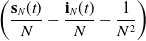 $\left ( \dfrac {\textbf s_N(t)}{N} - \dfrac {\textbf i_N(t)}{N} -\dfrac {1}{N^2} \right )$
,
 $ \left (\dfrac { \textbf i_N(t)}{N} \right )$
,
 $\left ( \dfrac {\textbf s_N(t)}{N} \right )$
. The associated small-time-interval probabilities are
 $N\beta _{SI} \textbf s_N(t)\textbf i_N(t)$
,
 $\lambda _{RS} N \textbf r_N(t)$
, and
 $( \gamma _{IH}+\gamma _{IR}+\gamma _{ID}) N \textbf i_N(t)$
. Therefore, the infinitesimal mean and variance can be obtained by summing the jump sizes (and their squares) weighted by the corresponding rates, which yields
 \begin{equation} \begin{aligned} \begin{cases} \mathscr{L}_{N} \left( \overrightarrow {\textbf {m}_N(t)} \right) = N\beta _{SI} \textbf s_N(t)\textbf i_N(t) \left ( \dfrac {\textbf s_N(t)}{N} - \dfrac {\textbf i_N(t)}{N} -\dfrac {1}{N^2} \right ) + \lambda _{RS} \textbf r_N(t) \textbf i_N(t) \\[3pt]\qquad\quad\quad\qquad -\, ( \gamma _{IH}+\gamma _{IR}+\gamma _{ID}) \textbf i_N(t) \textbf s_N(t), \\[3pt] \mathscr{W}_{N} \left( \overrightarrow {\textbf {m}_N(t)} \right) = N\beta _{SI} \textbf s_N(t)\textbf i_N(t) \left ( \dfrac {\textbf s_N(t)}{N} - \dfrac {\textbf i_N(t)}{N} -\dfrac {1}{N^2} \right ) ^2+ \lambda _{RS} N \textbf r_N(t) \left (\dfrac { \textbf i_N(t)}{N} \right ) ^2\\[3pt]\qquad\quad\quad\qquad +\, ( \gamma _{IH}+\gamma _{IR}+\gamma _{ID}) N \textbf i_N(t) \left ( \dfrac {\textbf s_N(t)}{N} \right ) ^2. \end{cases} \end{aligned} \end{equation}
A.4.2. Early time-step analysis for the stochastic instantaneous infection rate
We are now prepared to carry out a first-step analysis to examine the difference between the expectation of
 $\textbf {s} _N(t) \textbf {i} _N(t)$
and its deterministic counterpart
 $ {s} (t) {i} (t)$
.
By applying Eq. (A.12) over a small time interval
 $\Delta t$
, we obtain the following first-order approximation for the evolution of the stochastic instantaneous infection rate:
 \begin{equation} \textbf {s} _N(\Delta t + t) \textbf {i} _N(\Delta t + t) \approx \textbf {s} _N( t) \textbf {i} _N( t) + \mathscr{L} _{N} \left( \overrightarrow {\textbf {m}_N(t)} \right) \Delta t + \Delta \mathscr{O} _{N} \left( \overrightarrow {\textbf {m}_N(t)} \right )\!, \end{equation}
where
 $ { \Delta \mathscr{O}^{\kern1pt(l)}_{N} \left( \overrightarrow {\textbf {m}_N(t)} \right) } = { \mathscr{O}^{\kern1pt(l)}_{N} \left ( \overrightarrow {\textbf {m}_N(t + \Delta t)} \right ) }- { \mathscr{O}^{\kern1pt(l)}_{N} \left( \overrightarrow {\textbf {m}_N(t)} \right) }$
. Taking
 $t=0$
in Eq. (A.17), we infer that the stochastic instantaneous infection rate at the initial time admits the following first-step approximation over the interval
 $[0, \Delta t]$
:
 \begin{equation} \begin{aligned} \textbf {s}_{N}(\Delta t ) \textbf {i}_{N}(\Delta t ) &\approx \mathscr{L}_{N} \left (\overrightarrow {m}_{0N}\right ) \Delta t + \Delta \mathscr{O}_{N} \left (\overrightarrow {m}_{0N}\right ) + s _{0N}{i _{0N}} \\ &= {\mathscr{L}}_{N} \left (\overrightarrow {m}_{0N}\right ) \Delta t + {\mathscr{O}}_{N} \left (\overrightarrow {\textbf {m}_N(\Delta t)}\right ) + s _{0N}{i _{0N}} . \end{aligned} \end{equation}
Taking the variance on both sides of Eq. (A.18) and invoking Eq. (A.13), we obtain
 \begin{equation} \begin{aligned} {\operatorname {Var}}\left (\textbf {s} _{N}(\Delta t ) \textbf {i} _{N}(\Delta t ) \right ) \approx {\operatorname {Var}} \left ( {\mathscr{L} _{N} \left (\overrightarrow { {m}_{0N}} \right ) } \Delta t + \mathscr{O} _{N} \left ( \overrightarrow {\textbf {m}_N(\Delta t)} \right ) + {s _{0N}}{i _{0N} } \right ) = {\operatorname {Var}} \left ( \mathscr{O} _{N} \left ( \overrightarrow {\textbf {m}_N(\Delta t)} \right ) \right )\!. \end{aligned} \end{equation}
This, together with Eq. (A.14), implies that
 \begin{equation} \begin{aligned} {\operatorname {Var}}\left (\textbf {s} _{N}(\Delta t ) \textbf {i} _{N}(\Delta t ) \right ) \approx \mathbb{E}\left [\mathscr{W}_{N} \left (\overrightarrow { {m}_{0N}} \right ) \right ]\Delta t . \end{aligned} \end{equation}
We are now ready to perform a first-step analysis of the discrepancy between
 $\textbf {s} _N(t) \textbf {i} _N(t)$
and its deterministic counterpart
 $ {s} (t) {i} (t)$
. Taking the expectations on both sides of Eq. (A.18), we obtain
 \begin{equation} \mathbb E \left [ \textbf {s} _{N}(\Delta t ) \textbf {i} _{N}(\Delta t ) \right ] \approx \mathscr{L} _{N} \left ( \overrightarrow {\textbf {m}_N(0)} \right ) \Delta t +\mathbb E \left [ \Delta \mathscr{O} _{N} \left ( \overrightarrow {\textbf {m}_N(0)} \right ) \right ]+ {s _{0N}}{i _{0N}} = \mathscr{L} _{N} (0) \Delta t + {s _{0N}}{i _{0N}} . \end{equation}
We now compare
 $\mathbb E \left [ \textbf {s} _{N}(\Delta t ) \textbf {i} _{N}(\Delta t ) \right ]$
with its deterministic counterpart, namely
 $ {s} (\Delta t ) {i} (\Delta t )$
. From Eq. (3.2) and the product rule
 $\frac { \texttt {d} } {\texttt {d} t} (s(t) i (t) ) = s(t) \frac { \texttt {d} i (t) } {\texttt {d} t} + i (t) \frac { \texttt {d} s(t) } {\texttt {d} t}$
, it follows that the deterministic quantity
 $s(t)i(t)$
satisfies an integral formulation of the form
 \begin{equation} {s} (t) {i} (t) = {s }_{0 } {i}_{0 } + \int _{0}^{t} \mathscr{L} \left ( \overrightarrow { {m} (w)} \right ) dw , \end{equation}
where the drift
 $\mathscr{L} \left( \overrightarrow { {m} (t)} \right)$
is given by
 \begin{equation} \begin{aligned} {\mathscr{L} \left( \overrightarrow { {m} (t)} \right) } & = \beta _{SI} s (t) i (t) \left ( s (t) - i (t)\right ) +\lambda _{RS} r (t) i (t) - \left ( \gamma _{IH} + \gamma _{IR} + \gamma _{ID}\right ) i (t) s(t). \end{aligned} \end{equation}
Thus, we have
 \begin{equation} \begin{aligned} \mathscr{L}_{N} \left ( \overrightarrow {\textbf {m}_N(0)} \right ) & = \mathscr{L}_{N} \left ( \overrightarrow { {m}_{0N}} \right ) \\& = \beta _{SI} s_{0N} i_{0N} \left ( { s_{0N}} - { i_{0N}} -\dfrac {1}{N } \right ) + \lambda _{RS} r_{0N} i_{0N} - ( \gamma _{IH}+\gamma _{IR}+\gamma _{ID}) i_{0N} s _{0N} \\ & = \mathscr{L} \left ( \overrightarrow { {m}_{0N}} \right ) -\dfrac {1}{N} \beta _{SI} s_{0N} i_{0N} . \end{aligned} \end{equation}
This, together with Eq. (A.18) and the fact that the martingale has a mean of zero for every
 $t$
, implies that
 \begin{equation} \begin{aligned} \mathbb E \left [ \textbf {s} _{N}(\Delta t ) \textbf {i} _{N}(\Delta t ) \right ] &\approx \mathscr{L} _{N} \left ( \overrightarrow { {m}_{0N}} \right ) \Delta t + \mathbb E \left [ { \Delta \mathscr{O} _{N} \left ( \overrightarrow { {m}_{0N}} \right ) }\right ]+ {s _{0N}}{i _{0N}} \\ &= \mathscr{L} _{N} \left ( \overrightarrow { {m}_{0N}} \right ) \Delta t + {s _{0N}}{i _{0N}} \\ & = s ( \Delta t) i ( \Delta t) -\dfrac {1}{N} \beta _{SI} s_{0N} i_{0N}\Delta t . \end{aligned} \end{equation}
Moreover, with the above information, we are now in a position to estimate the discrepancy between
 $\mathbb E \left [ \mathscr{G}^{\kern1pt(l)}_{N} \left ( \overrightarrow {\textbf {m}_N(\Delta t)} \right ) \right ]$
and
 $ \mathscr{G}^{\kern1pt(l)} \left ( \overrightarrow { {m} (\Delta t)} \right )$
for
 $l = 1, 2$
. We first consider the case
 $l=1$
. From Eqs. (3.2), (3.7), and (A.25), we obtain
 \begin{equation} \begin{aligned} \mathbb E \left [ \mathscr{G}^{\kern1pt(1)}_{N} \left ( \overrightarrow {\textbf {m}_N(\Delta t)} \right ) \right ] & = -\beta _{SI} \mathbb E \left [ \textbf s_N(\Delta t) \textbf i_N(\Delta t) \right ] + \lambda _{RS} \mathbb E \left [\textbf r_N(\Delta t) \right ] \\ &= -\beta _{SI} \mathbb E \left [ \textbf s_N(\Delta t) \textbf i_N(\Delta t) \right ] + \lambda _{RS} r (\Delta t) \\ & \approx -\beta _{SI} \left ( s ( \Delta t) i ( \Delta t) -\dfrac {1}{N} \beta _{SI} s_{0N} i_{0N} \Delta t \right ) + \lambda _{RS} r (\Delta t) \\ &= \dfrac {\left (\beta _{SI} \right )^2}{N} s_{0N} i_{0N} \Delta t -\beta _{SI} s (\Delta t) i (\Delta t) + \lambda _{RS} r (\Delta t) \\ &= \dfrac {\left (\beta _{SI} \right )^2}{N} s_{0N} i_{0N} \Delta t + \left ( -\beta _{SI} s (\Delta t) i (\Delta t) + \lambda _{RS} r (\Delta t)\right ) \\ &= \dfrac {\left (\beta _{SI} \right )^2}{N} s_{0N} i_{0N} \Delta t + \mathscr{G}^{\kern1pt(1)} \left ( \overrightarrow { {m} (\Delta t)} \right )\!. \end{aligned} \end{equation}
Second, similarly for
 $l=2$
, by Eqs. (3.2), (3.7), and (A.25), we obtain
 \begin{equation} \begin{aligned} &\mathbb E \left [ \mathscr{G}^{\kern1pt(2)}_{N} \left ( \overrightarrow {\textbf {m}_N(\Delta t)} \right ) \right ] \\ &\quad = -\, ( \gamma _{IH}+\gamma _{IR}+\gamma _{ID}) \mathbb E \left [ \textbf i_N(\Delta t) \right ] + \beta _{SI} \mathbb E \left [\textbf s_N(\Delta t) \textbf i_N(\Delta t) \right ] \\ &\quad \approx -\, ( \gamma _{IH}+\gamma _{IR}+\gamma _{ID}) i (\Delta t) + \beta _{SI} \left ( s ( \Delta t) i ( \Delta t) -\dfrac {1}{N} \beta _{SI} s_{0N} i_{0N} \Delta t\right ) \\ &\quad = -\dfrac {\left (\beta _{SI} \right )^2}{N} s_{0N} i_{0N} \Delta t + \left ( - ( \gamma _{IH}+\gamma _{IR}+\gamma _{ID}) i (\Delta t) + \beta _{SI} s ( \Delta t) i ( \Delta t) \right ) \\ &\quad =- \dfrac {\left (\beta _{SI} \right )^2}{N} s_{0N} i_{0N} \Delta t + \mathscr{G}^{\kern1pt(2)} \left ( \overrightarrow { {m} (\Delta t)} \right )\!. \end{aligned} \end{equation}




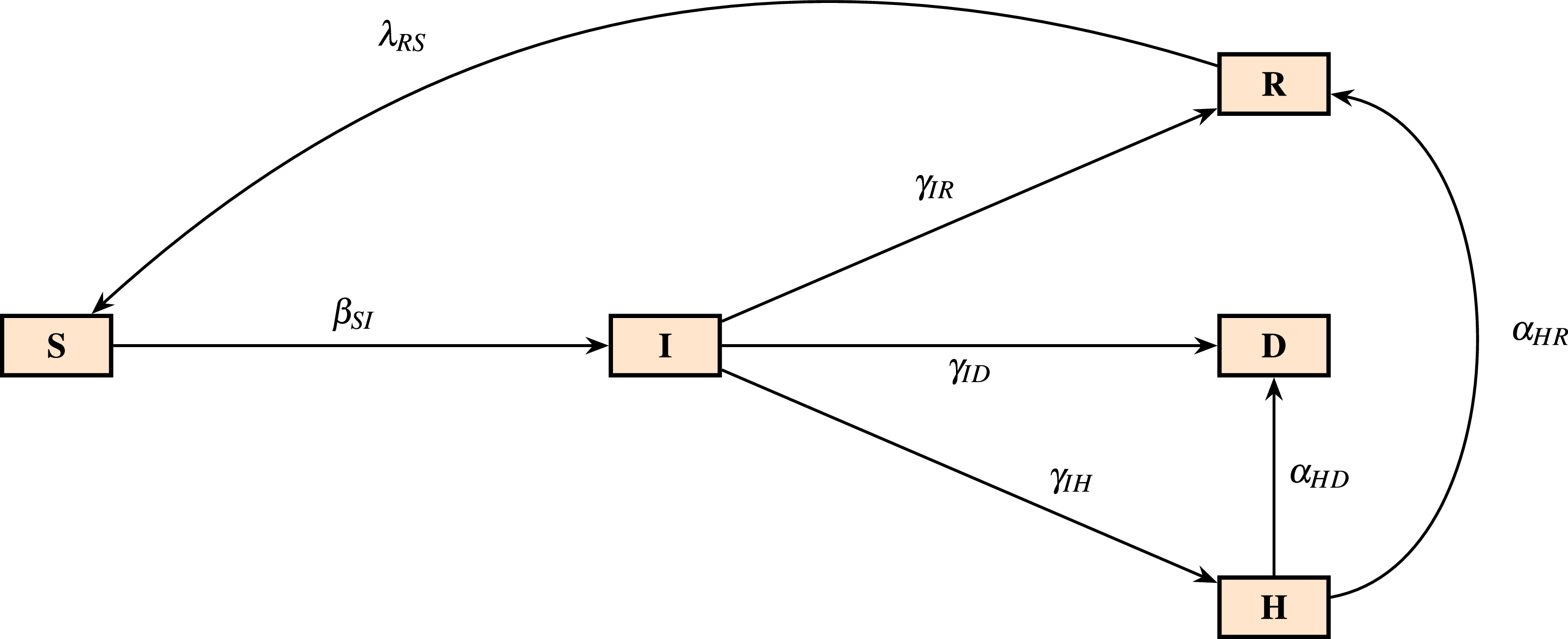

 N
 0
 1000
 (sN(t),rN(t))
 (iN(t),dN(t))
 hN(t)
 N=550
 1300
 2900
 7000
 t=0
 s0N=0.96
 i0N=0.035
 h0N=0.005

 N
 0
 1000


 N
 t∈[0,1000]
 N=15000
 30000
 60000

 ln(DN(l)(t))
 ln(RN(l)(t))
 t∈[5,1000]
 l=1,2,3,4,5
 N=550
 1300
 2900
 7000
 15000
 30000
 60000

 95%
 95%
 N=550
 7000
 60000

 logEN(l)(t)
 FN(l)(t)
 l=1,2,3,4,
 5
 N=550
 1300
 2900
 7000
 15000
 30000
 60000
 t∈[5,1000]
 t∈[0,1000]

 σ(mN(l)(t))
 l=1,2,3,4,
 5
 50%
 dN(t)
 N=550
 N=1300

 σ(mN(l)(t))
 l=1,2,3,4,
 5

 σ(MN(l)(t))
 σ(GN(l)(t))
 l=1,2,3,4,
 5
 N=550
 1300
 2900
 7000
 15000
 30000
 60000

 σ(GN(l)(t))
 l=1,2,3,4,
 5
 N=550
 1300
 2900
 7000
 15000
 30000
 60000

 N=58,639
 iN(t)
 90%
 i(t)
 hN(t)
 90%
 h(t)
 iN(t)
 hN(t)


 Open access

