





1. Introduction
Metamaterials are a class of artificial composite materials, typically comprising periodic or random arrays of subwavelength resonators [Reference Liu, Chan and Sheng26, Reference Matlack, Bauhofer, Krödel, Palermo and Daraio28]. These resonators are characterised by high contrasts between their specific physical parameters and those of the background medium. A ‘resonator’ is a device that amplifies waves via resonances at specific frequencies, a concept applicable to acoustic, electromagnetic and elastic waves. The ‘subwavelength’ means the incident wavelength is significantly larger than the resonator’s size. Metamaterials enable a range of exceptional applications, including super-resolution imaging [Reference Blåsten, Li, Liu and Wang12, Reference Casse, Lu, Huang, Gultepe, Menon and Sridhar14], super-focusing [Reference Ammari, Fitzpatrick, Gontier, Lee and Zhang5, Reference Lanoy, Pierrat, Lemoult, Fink, Leroy and Tourin21], waveguiding [Reference Alu and Engheta1, Reference Ammari, Hiltunen and Yu7], metasurfaces [Reference Ammari, Challa, Choudhury and Sini2, Reference Ammari, Fitzpatrick, Gontier, Lee and Zhang4] and invisibility cloaking [Reference Ammari, Ciraolo, Kang, Lee and Milton3, Reference Ando, Kang, Kim and Yu11, Reference Milton and Nicorovici29]. Due to these promising applications and feasible fabrication methods, the study of subwavelength resonances induced by high-contrast physical parameters has become a major research focus in recent decades.
In acoustics, bubbles embedded in a liquid can exhibit Minnaert resonance [Reference Ammari, Fitzpatrick, Gontier, Lee and Zhang6, Reference Feppon and Ammari19], a phenomenon resulting from the high density contrast between the gas and liquid. To improve bubble stability, an effective strategy is to replace the liquid with a soft elastic material featuring a small shear modulus [Reference Calvo, Thangawng and Layman13, Reference Chen, Gao, Li and Liu17]. Similarly, in electromagnetics, dielectric particles with high refractive indices function as subwavelength resonators [Reference Ammari, Li and Zou9, Reference Kuznetsov, Miroshnichenko, Brongersma, Kivshar and Luk’yanchuk20]. For elastic waves, both physical experiments and numerical simulations have confirmed that the lead ball coated with silicone rubber, characterised by high contrasts in Lamé parameters and density, exhibits localised resonant behaviour [Reference Liu, Chan and Sheng26, Reference Liu, Zhang, Mao, Zhu, Yang, Chan and Sheng27]. The authors in [Reference Chen, Gao, Li and Ren16] and [Reference Li and Zou25] independently utilised a variational method and layer potential techniques to develop a rigorous mathematical framework for elastic wave scattering and subwavelength resonant phenomena induced by high-contrast material parameters. A subsequent generalisation of this physical model, presented in [Reference Li and Xu24], replaced the single hard inclusion with two inclusions to enable the analysis of resonances and stress estimate.
The aforementioned references predominantly address the three-dimensional (3D) case. In this setting, the static single-layer potential operators – denoted by
 $\mathcal{S}_D$
for the Laplace equation and
 $\boldsymbol{\mathcal{S}}_D$
for the Lamé system – are always invertible [Reference Ammari, Kang and Lee8, Reference Chang and Choe15]. Moreover, these operators and their inverses are analytic with respect to the wavenumber
 $k$
in the low-frequency regime.
In contrast, the two-dimensional (2D) case introduces distinct mathematical challenges, which manifest in three key aspects:
-
1. The operators
 $\mathcal{S}_D$
and
$\boldsymbol{\mathcal{S}}_D$
may fail to be invertible. There exist bounded domains
$D$
for which
$\boldsymbol{\mathcal{S}}_D[\boldsymbol{\varphi }] = \boldsymbol 0$
for some non-trivial
$\boldsymbol{\varphi }$
. Notably, even for a disk, the kernel of
$\boldsymbol{\mathcal{S}}_D$
depends on its radius
$R$
[Reference Ando, Ji, Kang, Kim and Yu10]. A similar non-invertibility phenomenon for
$\mathcal{S}_D$
is also known [Reference Verchota32].
-
2. The asymptotic expansions of the fundamental solutions in the low-frequency regime differ significantly between the 2D and 3D cases. Specifically, the 3D expansion is a power series in
$k^j$
, while its 2D counterpart involves a double series comprising terms of the form
$k^{2j}$
and
$k^{2j} \ln k$
for
$j \in \mathbb{N}$
. -
3. The leading-order term in the asymptotic expansion of the single-layer potential operator is not simply the static operator. It also incorporates a logarithmic singularity
$\ln k$
and an imaginary component. We denote this leading-order term as
$\hat {\mathcal{S}}_D^k$
and
$\hat {\boldsymbol{\mathcal{S}}}_{D}^k$
for the Helmholtz equation and the Lamé system, respectively.


This complexity presents significant challenges for the mathematical investigation of subwavelength resonances in
 $\mathbb{R}^2$
. Notably, the equations governing the subwavelength resonant frequencies of 2D Minnaert bubbles are detailed for a single inclusion in the appendix of [Reference Ammari, Fitzpatrick, Gontier, Lee and Zhang6] and for two inclusions in [Reference Dong, Li and Xu18]. In contrast to acoustic waves (which are purely longitudinal), the investigation of elastic waves involves considerably higher complexity, attributable to the coupling of longitudinal and transverse waves as well as the vectorial characteristics of the Lamé operator. Furthermore, while the space spanned by all linear solutions to the Laplace equation with Neumann boundary conditions is one-dimensional, the corresponding space for the static Lamé system with Neumann boundary conditions is three-dimensional. These factors not only affect the invertibility of
 $\hat {\boldsymbol{\mathcal{S}}}^k_{D}$
but also lead to the leading-order terms of the resonant frequencies are governed by two
 $3\times 3$
matrices. Consequently, to rigorously establish the relationship between resonant frequencies and high-contrast parameters, this work focuses on the elastic scattering problem for resonators with radial geometry.
This paper extends the 3D high-contrast elastic scattering analysis from [Reference Chen, Gao, Li and Ren16] and [Reference Li and Zou25] to the more challenging 2D case. Unlike earlier approaches that employed primal and dual variational principles for the elastostatic system to identify resonant conditions [Reference Li and Liu22, Reference Li and Liu23], the works of [Reference Chen, Gao, Li and Ren16] and [Reference Ren, Chen, Gao and Li30] derived explicit expressions for subwavelength resonant frequencies by introducing the Dirichlet-to-Neumann (DtN) map and an auxiliary sesquilinear form. However, this variational approach is inapplicable in 2D case due to the lack of analyticity of the DtN map with respect to
 $k$
. To overcome this challenge, the present study adopts the boundary integral equations, leveraging the spectral properties of the Neumann–Poincaré (NP) operator. The main contributions are summarised as follows:
-
1. Asymptotic analysis of integral operators: Building on the asymptotic expansion of the zeroth-order Hankel function of the first kind, we establish the low-frequency asymptotic expressions for the relevant boundary integral operators with respect to the wavenumber
$k$
. Furthermore, we prove the invertibility of the leading-order operator
$\hat {\boldsymbol{\mathcal{S}}}^k_{D}$
in the case of
$\operatorname {Im} \ln k\neq \frac {\pi }{2}$
. In contrast to [Reference Li and Zou25], our definitions of fundamental solutions and associated operators are parameterised directly by
$k$
rather than by frequency. This choice leads to inherent differences in the analysis of both the boundary integral operators and the coefficients of the scattered fields. -
2. Reformulation via boundary integral equations and kernel analysis: The coupled internal–external scattering problem is reformulated as a system of boundary integral equations. The kernel space of the leading-order boundary integral operator is characterised by the spectral properties of
$\boldsymbol{\mathcal{S}}_D$
and the NP operator. This kernel space bifurcates into two distinct cases, contingent on the invertibility of
$\boldsymbol{\mathcal{S}}_D$
. We also determine the kernel space of the adjoint operator. Based on these kernel spaces, we introduce an invertible operator and then employ asymptotic analysis to derive the equations governing the leading-order terms of the resonant frequencies. In 3D case, these terms are explicitly given by the eigenvalues of a matrix, which is inherently symmetric. By contrast, explicit expressions in 2D are not always available even for a circular inclusion. -
3. Analysis of scattered fields: We explicitly derive the scattered field
$\boldsymbol u_D$
inside the resonator
$D$
for incident frequencies across different regimes. The enhancement coefficients of
$\boldsymbol u_D$
are of order
$\mathcal{O}(|\ln \omega |)$
and
$\mathcal{O}(|\omega ^{-1} \ln ^{-1} \omega |)$
, respectively, when the real incident frequency
$\omega$
is close to subwavelength resonances satisfying
$\omega ^2 \ln \omega = \mathcal{O}(\epsilon )$
and
$\omega ^2 = \mathcal{O}(\epsilon )$
. Here,
$\epsilon$
denotes the density contrast between the interior and exterior elastic materials. Additionally, we characterise the far-field patterns of the scattered field in the exterior domain, encompassing both longitudinal and transverse components. -
4. Subwavelength bandgap in dilute phononic crystals: Build upon the established existence of the subwavelength bandgap in phononic crystals [Reference Ren, Chen, Gao and Li30], we further pinpoint the exact frequency location of the bandgap within a dilute structure. This analysis exploits the small size of the resonator and the invertibility of
$\hat {\boldsymbol{\mathcal{S}}}^k_{D}$
. In this dilute regime, where the resonator size is much smaller than the inter-resonator distance, inter-particle interactions can be neglected.







This paper is structured into five main sections. Section 2 presents the mathematical formulation of the elastic scattering problem in
 $\mathbb{R}^2$
, introducing the definitions and fundamental properties of the relevant boundary integral operators. In Section 3, we derive the equations that govern the leading-order terms of the resonant frequencies. Section 4 analyzes the asymptotic behaviour of the scattered field inside the resonator and the corresponding far-field patterns when the incident frequency lies in different regimes. Section 5 examines the position of the subwavelength bandgap in dilute-structure phononic crystals. Finally, Section 6 provides concluding remarks and outlines future research directions.
2. Mathematical setup
This section is devoted to the mathematical characterisation of two-dimensional elastic wave scattering. We also present the definitions and essential properties of layer potential operators to establish the foundation for the subsequent analysis.
2.1. Problem formulation
Consider the two-dimensional elastic wave scattering by the scatterer
 $D$
, where
 $D$
is a disk with radius
 $R$
. Let the displacement field
 $\boldsymbol{u}=(u_i(\boldsymbol{x}))_{i=1}^2$
satisfy the time-harmonic Lamé system:
 \begin{align*} \mathcal{L}^{\widehat {\lambda },\widehat {\mu }} \boldsymbol{u}(\boldsymbol{x}) + \widehat {\rho } \, \omega ^2 \boldsymbol{u}(\boldsymbol{x}) = \boldsymbol 0, \quad \boldsymbol{x} \in \mathbb{R}^2, \end{align*}
where the partial differential operator
 $\mathcal{L}^{\widehat {\lambda },\widehat {\mu }}$
is defined by
 \begin{align*} \mathcal{L}^{\widehat {\lambda },\widehat {\mu }} \boldsymbol{u} \,:\!=\, \widehat {\mu } \, \nabla \cdot (\nabla \boldsymbol{u} + \nabla \boldsymbol{u}^\top ) + \widehat {\lambda } \, \nabla (\nabla \cdot \boldsymbol{u}) \end{align*}
with
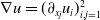 $\nabla \boldsymbol{u} = (\partial _{x_j} u_i)_{i,j=1}^2$
denoting the displacement gradient matrix and
 ${}^\top$
denoting the matrix transpose. Define the conormal derivative
 $\partial _{\boldsymbol{\nu };\,\widehat {\lambda },\widehat {\mu }}$
as
 \begin{align} \partial _{\boldsymbol{\nu };\,\widehat {\lambda },\widehat {\mu }}\boldsymbol{u}\,:\!=\,\widehat {\lambda }(\nabla \cdot \boldsymbol{u})\boldsymbol{\nu }+\widehat {\mu }(\nabla \boldsymbol{u}+\nabla \boldsymbol{u}^\top )\boldsymbol{\nu } \end{align}
with
 $\boldsymbol{\nu }$
representing the unit outward normal vector to
 $\partial D$
. The material parameters – the density
 $\widehat {\rho }$
and the Lamé parameters
 $\widehat {\lambda }$
and
 $\widehat {\mu }$
– are piecewise constant, defined by
 \begin{align*} (\widehat {\rho };\, \mathbb{R}^2) =(\rho ;\, \mathbb{R}^2\backslash \overline {D}) \cup (\widetilde {\rho };\, D) , \quad (\widehat {\lambda }, \widehat {\mu };\, \mathbb{R}^2) = (\lambda , \mu ;\, \mathbb{R}^2 \backslash \overline {D}) \cup (\widetilde {\lambda }, \widetilde {\mu };\, D) . \end{align*}
These parameters satisfy the strong convexity conditions in both media
 \begin{align*} \mu \gt 0, \quad \lambda + \mu \gt 0, \quad \widetilde {\mu } \gt 0, \quad \text{and} \quad \widetilde {\lambda } + \widetilde {\mu } \gt 0. \end{align*}
The corresponding shear and compressional wave velocities in the exterior domain
 $\mathbb{R}^2 \backslash \overline {D}$
and the inclusion
 $D$
are given, respectively
 \begin{align} \begin{cases} c_s = \sqrt {\mu / \rho }, \\[3pt] c_p = \sqrt {(\lambda + 2\mu ) / \rho }, \end{cases} \quad \text{and} \quad \begin{cases} \widetilde {c}_s = \sqrt {\vphantom{\sum}\widetilde {\mu } / \widetilde {\rho }}, \\[3pt] \widetilde {c}_p = \sqrt {\vphantom{\sum}(\widetilde {\lambda } + 2\widetilde {\mu }) / \widetilde {\rho }}. \end{cases} \end{align}
Consider the time-harmonic incident wave
 $\boldsymbol{u}^{\mathrm{in}}$
(with the frequency
 $\omega$
) that is scattered by
 $D$
. The resulting total field
 $\boldsymbol{u}$
is governed by the following Lamé system:
 \begin{align} \left \{ \kern-3pt\begin{aligned} &\mathcal{L}^{\lambda ,\mu }\boldsymbol{u}+\rho \omega ^2\boldsymbol{u}= \boldsymbol 0&&\text{in }\mathbb{R}^2\backslash \overline {D},\\ &\mathcal{L}^{\widetilde {\lambda },\widetilde {\mu }}\boldsymbol{u}+\widetilde {\rho }\omega ^2\boldsymbol{u}=\boldsymbol 0&&\text{in } D,\\ &\boldsymbol{u}|_+=\boldsymbol{u}|_-&&\text{on } \partial D,\\ &\partial _{\boldsymbol{\nu };\,\lambda ,\mu }\boldsymbol{u} \big |_+=\partial _{\boldsymbol{\nu };\,\widetilde {\lambda },\widetilde {\mu }}\boldsymbol{u}\big |_-&&\text{on }\partial D, \end{aligned}\right . \end{align}
where the notations
 $|_{+}$
and
 $|_{-}$
denote the traces on
 $\partial D$
taken from outside and inside of
 $D$
, respectively. To ensure that the scattering wave propagates outwards, the following Kupradze radiation conditions are imposed at infinity [Reference Ammari, Kang and Lee8]:
 \begin{align*} \left \{ \kern-3pt\begin{aligned} &(\nabla \times \nabla \times (\boldsymbol{u}-\boldsymbol{u}^{\mathrm{in}}))(\boldsymbol x)\times \frac {\boldsymbol x}{|\boldsymbol x|}-\mathrm{i}k_s\nabla \times (\boldsymbol{u}-\boldsymbol{u}^{\mathrm{in}})(\boldsymbol x)=\mathcal{O}\big(|\boldsymbol x|^{-\frac {3}{2}}\big)& \text{as }|\boldsymbol x|\rightarrow +\infty ,\\ &\frac {\boldsymbol x}{|\boldsymbol x|}\cdot (\nabla (\nabla \cdot (\boldsymbol{u}-\boldsymbol{u}^{\mathrm{in}})))(\boldsymbol x)-\mathrm{i}k_p\nabla \cdot (\boldsymbol{u}-\boldsymbol{u}^{\mathrm{in}})(\boldsymbol x)=\mathcal{O}\big(|\boldsymbol x|^{-\frac {3}{2}}\big)&\text{as }|\boldsymbol x|\rightarrow +\infty , \end{aligned}\right . \end{align*}
where
 \begin{align} k_s=\frac {\omega }{c_s}\quad \text{and}\quad k_p=\frac {\omega }{c_p} \end{align}
denote the shear wavenumber and compressional wavenumber, respectively.
To quantify the discrepancy between the material parameters of the inclusion
 $D$
and the background medium
 $\mathbb{R}^2 \backslash \overline {D}$
, we introduce the following dimensionless contrast parameters:
 \begin{align} (\widetilde {\lambda },\widetilde {\mu })=\frac {1}{\delta }(\lambda ,\mu ), \quad \widetilde {\rho }=\frac {1}{\epsilon }\rho , \quad \tau =\frac {c_s}{\widetilde {c}_s}=\frac {c_p}{\widetilde {c}_p}. \end{align}
In view of the wave speeds defined in (2.2), the parameter
 $\tau$
satisfies the relation
 \begin{align} \tau =\sqrt {\frac {\delta }{\epsilon }}. \end{align}
Using the relations in (2.5) and (2.6), the system (2.3) can be reformulated equivalently as
 \begin{align} \left \{ \kern-2pt\begin{aligned} &\mathcal{L}^{\lambda ,\mu }\boldsymbol{u}+\rho \omega ^2\boldsymbol{u}=\boldsymbol 0&&\text{in }\mathbb{R}^2\backslash \overline {D},\\ &\mathcal{L}^{\lambda ,\mu }\boldsymbol{u}+\rho \tau ^2\omega ^2\boldsymbol{u}= \boldsymbol 0&&\text{in } D,\\ &\boldsymbol{u}|_+=\boldsymbol{u}|_-&&\text{on } \partial D,\\ &\delta \partial _{ \boldsymbol{\nu }} \boldsymbol{u}\big |_+=\partial _{\boldsymbol{\nu }}\boldsymbol{u}\big |_-&&\text{on }\partial D. \end{aligned}\right . \end{align}
Here, we abbreviate
 $\partial _{ \boldsymbol{\nu }}\boldsymbol{u}=\partial _{\boldsymbol{\nu };\,\lambda ,\mu }\boldsymbol{u}$
, with
 $\partial _{\boldsymbol{\nu };\,\lambda ,\mu }\boldsymbol{u}$
given by (2.1).
The subsequent analysis relies on the following physical assumptions:
-
• High contrasts: the scatterer’s Lamé parameters and density differ significantly from the background medium (
$\delta , \epsilon \to 0^+$
). -
• Matched wave speeds: the wave speeds inside and outside are of the same order (
$\tau = \mathcal{O}(1)$
). -
• Subwavelength regime: the exciting frequency is small (
$\omega \to 0$
).


2.2. Layer potential operators
In this subsection, we present the definitions of layer potential operators and derive the asymptotic expansions of these operators in the low-frequency regime.
For the wavenumber
 $k$
, define the single-layer potential
 $\boldsymbol{\widetilde {\mathcal{S}}}^{\,k}_{D}\,:\, L^2(\partial D)^2\rightarrow H^{3/2}_{\mathrm{loc}}(\mathbb{R}^2)^2$
as
 \begin{align*} \boldsymbol{\widetilde {\mathcal{S}}}^{k}_{D}[\boldsymbol \varphi ](\boldsymbol x)\,:\!=\,\int _{\partial D}\boldsymbol{G}^{k}(\boldsymbol x-\boldsymbol y)\boldsymbol \varphi (\kern1pt\boldsymbol y)\mathrm{d}\sigma (\kern1pt\boldsymbol y),\quad \boldsymbol x\in \mathbb{R}^2\backslash \partial D, \end{align*}
where the Green’s tensor
 $\boldsymbol{G}^{k}(\boldsymbol x-\boldsymbol y)$
is the fundamental solution to
 \begin{align*} (\mathcal{L}^{\lambda ,\mu }+k^2)\boldsymbol{G}^{k}(\boldsymbol x-\boldsymbol y)=\boldsymbol{\delta }(\boldsymbol x-\boldsymbol y)\boldsymbol{I}. \end{align*}
Here,
 $\boldsymbol{\delta }$
denotes the Dirac delta distribution and
 $\boldsymbol{I}$
is the
 $2\times 2$
identity matrix. Explicitly, the fundamental solution
 $\boldsymbol{G}^{k}(\boldsymbol x)=(G_{ij}^{k}(\boldsymbol x))^2_{i,j=1}$
is given by
 \begin{equation} \begin{aligned} G_{ij}^{k}(\boldsymbol x)=\begin{cases}\frac {1}{4\pi }\big(\frac {1}{\mu }+\frac {1}{\lambda +2\mu }\big)\delta _{ij}\ln |\boldsymbol x|-\frac {1}{4\pi }\big(\frac {1}{\mu }-\frac {1}{\lambda +2\mu }\big)\frac {x_{i}x_{j}}{|\boldsymbol x|^{2}},&k=0,\\[5pt] -\frac {\mathrm{i}}{4\mu }\delta _{ij}H_{0}^{(1)}\left (\frac {k|\boldsymbol x|}{\sqrt {\mu }}\right )+\frac {\mathrm{i}}{4k^{2}}\partial _{i}\partial _{j} \Big(H_{0}^{(1)}\Big(\frac {k|\boldsymbol x|}{\sqrt {\lambda +2\mu }}\Big)-H_{0}^{(1)}\Big(\frac {k|\boldsymbol x|}{\sqrt {\mu }}\Big)\Big),&k\neq 0, \end{cases} \end{aligned} \end{equation}
where
 $H_{0}^{(1)}$
denotes the zeroth-order Hankel function of the first kind and
 $x_i$
is the
 $i$
-th component of the vector
 $\boldsymbol x$
.
With the fundamental solution
 $\boldsymbol{G}^{k}(\boldsymbol x)$
defined piecewise for
 $k=0$
and
 $k\neq 0$
in (2.8), we further define the boundary integral operators
 $\boldsymbol{\mathcal{S}}^{k}_{D}\,:\, L^2(\partial D)^2\rightarrow H^{1}(\partial D)^2$
and
 $\boldsymbol{\mathcal{K}}^{k,*}_{D}\,:\, L^2(\partial D)^2\rightarrow L^2(\partial D)^2$
as
 \begin{align*} \boldsymbol{\mathcal{S}}^{k}_{D}[\boldsymbol \varphi ](\boldsymbol x)&\,:\!=\,\int _{\partial D}\boldsymbol G^{k}(\boldsymbol x-\boldsymbol y)\boldsymbol \varphi (\kern1pt\boldsymbol y)\mathrm{d}\sigma (\kern1pt\boldsymbol y),\quad \boldsymbol x\in \partial {D},\\[4pt] \boldsymbol{\mathcal{K}}^{k,*}_{D}[\boldsymbol \varphi ](\boldsymbol x)&\,:\!=\,\mathrm{p.v.}\int _{\partial D} \partial _{\boldsymbol{\nu }_{\boldsymbol x}}\boldsymbol G^{k}(\boldsymbol x-\boldsymbol y)\boldsymbol \varphi (\kern1pt\boldsymbol y)\mathrm{d}\sigma (\kern1pt\boldsymbol y),\quad \boldsymbol x\in \partial {D}, \end{align*}
where
 $\mathrm{p.v.}$
denotes the Cauchy principal value and
 $\boldsymbol{\mathcal{K}}^{k,*}_{D}$
is referred to as NP operator. For
 $k=0$
, the above operators adopt the static fundamental solution
 $\boldsymbol{G}^{0}$
and are denoted simply by
 $\boldsymbol{\mathcal{S}}_{D}$
and
 $\boldsymbol{\mathcal{K}}^{*}_{D}$
. Moreover, the following jump relations hold
 \begin{align} \partial _{\boldsymbol{\nu }}\boldsymbol{\mathcal{S}}^{k}_{D}[\boldsymbol \varphi ]\big |_{\pm }(\boldsymbol x)=\left (\pm \frac {1}{2}\boldsymbol{\mathcal{I}}+\boldsymbol{\mathcal{K}}^{k,*}_{ D}\right )[\boldsymbol \varphi ](\boldsymbol x),\quad \boldsymbol x\in \partial {D} \end{align}
with the identity operator
 $\boldsymbol{\mathcal{I}}$
.
Introduce four parameters
 \begin{align} \tau _1&=\frac {1}{2}\left (\frac {1}{\mu }+\frac {1}{\lambda +2\mu }\right )\!,&&\tau _2=\frac {1}{2}\left (\frac {1}{\mu }-\frac {1}{\lambda +2\mu }\right )\!,\nonumber \\[5pt] \varrho _1&=-\frac {1}{8\pi }\left (\gamma -\ln 2-\frac {\mathrm{i}\pi }{2}-1\right )\!,&&\varrho _2=\frac {1}{128\pi }\left (\gamma -\ln 2-\frac {\mathrm{i}\pi }{2}-\frac {3}{2}\right ) \end{align}
with the Euler’s constant
 $\gamma$
.
Next, we derive the asymptotic expansions of
 $\boldsymbol{\mathcal{S}}^{k}_{D}$
and
 $\boldsymbol{\mathcal{K}}^{k,*}_{D}$
with respect to
 $k$
as
 $k\rightarrow 0$
, based on the asymptotic expansion of
 $\boldsymbol G^k$
.
Lemma 2.1.
As
 $k\rightarrow 0$
, the fundamental solution
 $\boldsymbol G^k$
admits the asymptotic expansion
 \begin{align*} \boldsymbol G^{k}(\boldsymbol x)= \boldsymbol G^{0}(\boldsymbol x)+ \beta _k \boldsymbol I + k^2 \ln k \boldsymbol A(\boldsymbol x)+k^2 \boldsymbol B(\boldsymbol x)+\mathcal{O}(k^4 \ln k+k^4), \end{align*}
where
 $\boldsymbol A(\boldsymbol x)=(a_{ij}(\boldsymbol x))^2_{i,j=1},$
 $\boldsymbol B(\boldsymbol x)=(b_{ij}(\boldsymbol x))^2_{i,j=1},$
and
 \begin{align} \beta _k = \frac {\tau _1}{4\pi }(2\gamma - \pi \mathrm{i} - \ln 4) + \frac {\tau _2}{4\pi } + \frac {\ln (k/\sqrt {\lambda +2\mu })}{4\pi (\lambda + 2\mu )} + \frac {\ln (k/\sqrt {\mu })}{4\pi \mu }. \end{align}
Here, the matrix elements are given by
 \begin{align*} &a_{ij}(\boldsymbol x)=\delta _{ij}\left (-\frac {3|\boldsymbol x|^2}{32\pi \mu ^2}-\frac {|\boldsymbol x|^2}{32\pi (\lambda +2\mu )^2}\right )-\frac {x_ix_j}{16\pi (\lambda +2\mu )^2}+\frac {x_ix_j}{16\pi \mu ^2},\\[5pt] &b_{ij}(\boldsymbol x)=\delta _{ij}\left (\sigma _1|\boldsymbol x|^2+(\tau _1 \tau _2-\mu ^{-2})\frac {|\boldsymbol x|^2\ln |\boldsymbol x|}{8\pi }\right )+\sigma _2x_ix_j+\frac {\tau _1\tau _2}{4\pi }x_ix_j\ln |\boldsymbol x| \end{align*}
with the constants given by
 \begin{align*} &\sigma _1=\frac {1}{\mu ^2}\left (\varrho _1{+\frac {3\ln \mu }{64\pi }}+4\varrho _2+\frac {1}{128\pi }\right )-\frac {1}{(\lambda +2\mu )^2}\left (4\varrho _2+\frac {1}{128\pi }-\frac {\ln (\lambda +2\mu )}{64\pi }\right )\!,\\[5pt] &\sigma _2=\frac {8}{\mu ^2}\left (\varrho _2-\frac {\ln \mu }{256\pi }\right )-\frac {8}{(\lambda +2\mu )^2}\left (\varrho _2-\frac {\ln (\lambda +2\mu )}{256\pi }\right )+\frac {3\tau _1\tau _2}{16\pi }. \end{align*}
Proof. Using the following behaviour of the Hankel function
 $H_{0}^{(1)}$
near
 $0$
(cf. [Reference Ammari, Kang and Lee8, p. 22]):
 \begin{align*} -\frac {\mathrm{i}}{4}H_{0}^{(1)}(k|\boldsymbol x|)=&\frac {1}{2\pi }\ln |\boldsymbol x|+\frac {1}{2\pi }({\ln}\, k+\gamma -\ln 2)-\frac {\mathrm{i}}{4}+\left (-\frac {1}{8\pi }\ln (k|\boldsymbol x|)+\varrho _1\right )(k|\boldsymbol x|)^2\\[3pt] &+\left (\frac {1}{128\pi }\ln (k|\boldsymbol x|)+\varrho _2\right )(k|\boldsymbol x|)^4+\mathcal{O}(k^6 \ln k+k^6), \quad \text{for }k\ll 1. \end{align*}
By substituting this expansion into the expression for
 $\boldsymbol{G}^k$
given by (2.8) and performing careful term-by-term computation, we can obtain the desired asymptotic expansion.
Lemma 2.2.
As
 $k\rightarrow 0$
, the boundary integral operators
 $\boldsymbol{\mathcal{S}}^{k}_{D}\,:\, L^{2}(\partial D)^2\rightarrow H^{1}(\partial D)^2$
and
 $\boldsymbol{\mathcal{K}}^{k,*}_{D}\,:\,L^{2}(\partial D)^2\rightarrow L^{2}(\partial D)^2$
admit the following asymptotic expansions:
 \begin{align*} \boldsymbol{\mathcal{S}}^{k}_{D}=\hat {\boldsymbol{\mathcal{S}}}^k_{D}+k^2\ln k \boldsymbol{\mathcal{S}}^{(1)}_{D,1}+k^2\boldsymbol{\mathcal{S}}^{(2)}_{D,1}+\mathcal{O}(k^4\ln k+k^4), \end{align*}
 \begin{align*} \boldsymbol{\mathcal{K}}^{k,*}_{D}=\boldsymbol{\mathcal{K}}^*_{D}+k^2\ln k \boldsymbol{\mathcal{K}}^{(1),*}_{D,1}+k^2\boldsymbol{\mathcal{K}}^{(2),*}_{D,1}+\mathcal{O}(k^4\ln k+k^4), \end{align*}
where
 \begin{align} \hat {\boldsymbol{\mathcal{S}}}^k_{D}[\boldsymbol \varphi ]=\boldsymbol{\mathcal{S}}_{D}[\boldsymbol \varphi ]+\beta _k\int _{\partial D}\boldsymbol \varphi (\kern1pt\boldsymbol y)\mathrm{d}\sigma (\kern1pt\boldsymbol y), \end{align}
 \begin{equation*}\boldsymbol{\mathcal{S}}^{(1)}_{D,1}[\boldsymbol \varphi ]=\int _{\partial D}\boldsymbol A(\boldsymbol x-\boldsymbol y)\boldsymbol \varphi (\kern1pt\boldsymbol y)\mathrm{d}\sigma (\kern1pt\boldsymbol y),\quad \boldsymbol{\mathcal{S}}^{(2)}_{D,1}[\boldsymbol \varphi ]=\int _{\partial D}\boldsymbol B(\boldsymbol x-\boldsymbol y)\boldsymbol \varphi (\kern1pt\boldsymbol y)\mathrm{d}\sigma (\kern1pt\boldsymbol y),\end{equation*}
and
 \begin{equation*}\boldsymbol{\mathcal{K}}^{(1),*}_{D,1}[\boldsymbol \varphi ]=\int _{\partial D}\partial _{\boldsymbol{\nu }_{\boldsymbol x}}\boldsymbol A(\boldsymbol x-\boldsymbol y)\boldsymbol \varphi (\kern1pt\boldsymbol y)\mathrm{d}\sigma (\kern1pt\boldsymbol y),\quad \boldsymbol{\mathcal{K}}^{(2),*}_{D,1}[\boldsymbol \varphi ]=\int _{\partial D}\partial _{\boldsymbol{\nu }_{\boldsymbol x}}\boldsymbol B(\boldsymbol x-\boldsymbol y)\boldsymbol \varphi (\kern1pt\boldsymbol y)\mathrm{d}\sigma (\kern1pt\boldsymbol y)\end{equation*}
with
 $\beta _k$
,
 $\boldsymbol A$
and
 $\boldsymbol B$
defined in Lemma 2.1
.
Consider the following homogeneous Neumann problem for the Lamé system:
 \begin{align*} \begin{cases} \mathcal{L}^{\lambda ,\mu } \boldsymbol u = \boldsymbol 0 & \text{in } D, \\ \partial _{\boldsymbol \nu } \boldsymbol u = \boldsymbol 0 & \text{on } \partial D. \end{cases} \end{align*}
The solution space of this problem is spanned by three linearly independent functions
 \begin{align} \boldsymbol f^{(1)} = \frac {1}{\sqrt {2\pi R}} \begin{pmatrix} 1 \\ 0 \end{pmatrix}\!, \quad \boldsymbol f^{(2)} = \frac {1}{\sqrt {2\pi R}} \begin{pmatrix} 0 \\ 1 \end{pmatrix}\!, \quad \boldsymbol f^{(3)} = \frac {1}{\sqrt {2\pi R^3}} \begin{pmatrix} x_2 \\ -x_1 \end{pmatrix}\!, \end{align}
where
 $x_i$
denotes the
 $i$
-th component of
 $\boldsymbol x\in D$
. Obviously, these basis functions are orthonormal in
 $L^2(\partial D)^2$
, satisfying
 \begin{align} \langle \kern1.9pt\boldsymbol f^{(i)},\boldsymbol f^{(j)}\rangle =\delta _{ij}, \quad \text{for } i, j =1, 2, 3, \end{align}
where
 $\langle \cdot ,\cdot \rangle$
denotes the inner product in
 $L^2(\partial D)^2$
. Furthermore, we introduce the spaces
 \begin{equation*}\mathcal{H}=L^2(\partial D)^2\times L^2(\partial D)^2\end{equation*}
and
 \begin{equation*}\mathcal{H}_1=H^1(\partial D)^2\times L^2(\partial D)^2.\end{equation*}
Define a subspace of
 $L^2(\partial D)^2$
by
 \begin{equation*}\mathbf{L}^2_{\boldsymbol f}(\partial D)=\{\boldsymbol h\in L^2(\partial D)^2\,:\,\langle \boldsymbol h,\boldsymbol f^{(i)}\rangle =0, \forall i=1,2,3\}.\end{equation*}
Lemma 2.3. (see [ Reference Ando, Ji, Kang, Kim and Yu10 ]) One has
-
(i) The operator
$\boldsymbol{\mathcal{S}}_{D}$
is invertible in the subspace
$\mathbf{L}^2_{\boldsymbol f}(\partial D)$
. -
(ii) The eigenvectors
$\boldsymbol f^{(1)},\boldsymbol f^{(2)}$
and
$\boldsymbol f^{(3)}$
span the eigenspace for the operator
$\boldsymbol{\mathcal{K}}_{D}$
in
$ L^{2}(\partial D)^2$
corresponding to the eigenvalue
$\frac {1}{2}$
, where
$\boldsymbol{\mathcal{K}}_{D}$
is the
$L^2$
-adjoint of
$\boldsymbol{\mathcal{K}}^{*}_{D}$
. -
(iii) When
$D$
is a disk, the eigenvectors
$\boldsymbol f^{(1)},\boldsymbol f^{(2)}$
and
$\boldsymbol f^{(3)}$
span the eigenspace for the operator
$\boldsymbol{\mathcal{K}}^*_{D}$
in
$ L^{2}(\partial D)^2$
corresponding to the eigenvalue
$\frac {1}{2}$
.


Lemma 2.4.
Let
 $D$
be a disk of radius
 $R$
. Then the operator
 $\widetilde {\boldsymbol{\mathcal{S}}}_{D}$
satisfies the following identities:
-
(i)
$\widetilde {\boldsymbol{\mathcal{S}}}_{D}[\kern1.4pt\boldsymbol f^{(1)}]=\left (\tau _1 R\ln R-\frac {\tau _2}{2} R\right )\boldsymbol f^{(1)},$
-
(ii)
$\widetilde {\boldsymbol{\mathcal{S}}}_{D}[\kern1.4pt\boldsymbol f^{(2)}]=\left (\tau _1 R\ln R-\frac {\tau _2}{2} R\right )\boldsymbol f^{(2)},$
-
(iii)
$\widetilde {\boldsymbol{\mathcal{S}}}_{D}[\kern1.4pt\boldsymbol f^{(3)}]=-\frac {R}{2\mu }\boldsymbol f^{(3)},$



where
 $\tau _1$
and
 $\tau _2$
are constants defined by (2.10).
Proof. We begin with the following identities from [Reference Ammari, Ciraolo, Kang, Lee and Milton3]:
 \begin{align} \int _{\partial D}\frac {1}{2\pi }\ln |\boldsymbol x-\boldsymbol y|\mathrm{d}\sigma (\kern1pt\boldsymbol y)=R\ln R \quad \text{and}\quad \int _{\partial D}\frac {1}{2\pi }\ln |\boldsymbol x-\boldsymbol y|y_i\mathrm{d}\sigma (\kern1pt\boldsymbol y)=-\frac {R x_i}{2}, \quad \text{for } \boldsymbol x\in D. \end{align}
For
 $i = 1,2$
, we can obtain
 \begin{align*} \int _{\partial D} \frac {1}{2\pi } \frac {(x_i-y_i)^2}{|\boldsymbol x-\boldsymbol y|^2}\mathrm{d}\sigma (\kern1pt\boldsymbol y)&=x_i \int _{\partial D} \frac {1}{2\pi } \frac {x_i-y_i}{|\boldsymbol x-\boldsymbol y|^2}\mathrm{d}\sigma (\kern1pt\boldsymbol y) - \int _{\partial D} \frac {1}{2\pi } \frac {(x_i-y_i)y_i}{|\boldsymbol x-\boldsymbol y|^2}\mathrm{d}\sigma (\kern1pt\boldsymbol y)\\ &=x_i\partial _{x_i}\int _{\partial D}\frac {1}{2\pi }\ln |\boldsymbol x-\boldsymbol y|\mathrm{d}\sigma (\kern1pt\boldsymbol y)-\partial _{x_i}\int _{\partial D}\frac {1}{2\pi }\ln |\boldsymbol x-\boldsymbol y|y_i\mathrm{d}\sigma (\kern1pt\boldsymbol y)\\ &=\frac {R}{2}, \end{align*}
and
 \begin{align} &\int _{\partial D} \frac {1}{2\pi } \frac {(x_1-y_1)(x_2-y_2)}{|\boldsymbol x-\boldsymbol y|^2}\mathrm{d}\sigma (\kern1pt\boldsymbol y)\nonumber \\[3pt]& \quad =x_2 \partial _{x_1}\int _{\partial D} \frac {1}{2\pi } \ln |\boldsymbol x-\boldsymbol y|\mathrm{d}\sigma (\kern1pt\boldsymbol y) - \partial _{x_1}\int _{\partial D} \frac {1}{2\pi }\ln |\boldsymbol x-\boldsymbol y|y_2 \mathrm{d}\sigma (\kern1pt\boldsymbol y)\nonumber \\[3pt]& \quad = 0. \end{align}
Then, (i) and (ii) follows directly from the definition of
 $\widetilde {\boldsymbol{\mathcal{S}}}_{D}$
and the above computations.
Moreover, it follows from polar coordinate calculations that
 \begin{align*} \int _{\partial D}\frac {1}{2\pi }\frac {(\boldsymbol x-\boldsymbol y)(\boldsymbol x-\boldsymbol y)^\top }{|\boldsymbol x-\boldsymbol y|^2}\begin{pmatrix} y_2 \\ -y_1 \end{pmatrix} \mathrm{d}\sigma (\kern1pt\boldsymbol y) = \frac {R}{2} \begin{pmatrix} x_2 \\ -x_1 \end{pmatrix}\!,\quad \text{for } \boldsymbol x\in D. \end{align*}
Combining these with (2.15) yields (iii).
Let
 \begin{align} \Delta = \tau _1 R \ln R - \frac {\tau _2}{2} R. \end{align}
According to Lemma 2.4, the invertibility of the operator
 $ \boldsymbol{\mathcal{S}}_D$
is determined by the value of
 $ \Delta$
. Throughout this paper, we shall distinguish the following two cases:
-
• The non-invertible case:
$ \Delta = 0$
, where
$ \boldsymbol{\mathcal{S}}_D$
is clearly not invertible
$(\boldsymbol{\mathcal{S}}_{D}[\kern1.4pt\boldsymbol f^{(1)}]=\boldsymbol{\mathcal{S}}_{D}[\kern1.4pt\boldsymbol f^{(2)}]=\boldsymbol 0)$
; -
• The invertible case:
$ \Delta \neq 0$
, where
$ \boldsymbol{\mathcal{S}}_D$
is invertible (by property (i) in Lemma 2.3).





In all subsequent lemmas, theorems, and formulas, these two cases will be referred to explicitly by the conditions
 $ \Delta = 0$
and
 $ \Delta \neq 0$
, respectively.
3. Subwavelength resonances
This section utilises boundary integral equations to reformulate the scattering problem (2.7). Based on the kernel space of the leading-order operator, we construct an auxiliary invertible operator. The subwavelength resonant frequencies are subsequently derived through the asymptotic analysis, which are closely linked to the diagonal elements of the two diagonal matrices. Towards this goal, our first step is to demonstrate that the leading-order term
 $\hat {\boldsymbol{\mathcal{S}}}^k_{D}$
of the boundary integral operator
 $\boldsymbol{\mathcal{S}}^{k}_{D}$
is invertible and that the two matrices are indeed diagonal.
Lemma 3.1.
Let
 $D$
be a disk of radius
 $R$
. For any
 $k\in \mathbb{C}$
with
 $\operatorname {Im}\ln k\neq \frac {\pi }{2}$
, the operator
 $\hat {\boldsymbol{\mathcal{S}}}^k_{D}\,:\,L^{2}(\partial D)^2\rightarrow H^{1}(\partial D)^2$
defined in (2.12) is invertible.
Proof. Let us first demonstrate the injectivity of the operator
 $\hat {\boldsymbol{\mathcal{S}}}^k_{D}.$
Suppose
 $\boldsymbol \varphi \in L^2(\partial D)^2$
satisfies
 \begin{align} \hat {\boldsymbol{\mathcal{S}}}^k_{D}[\boldsymbol \varphi ]=\boldsymbol{\mathcal{S}}_{D}[\boldsymbol \varphi ]+\beta _k\int _{\partial D}\boldsymbol \varphi (\kern1pt\boldsymbol y)\mathrm{d}\sigma (\kern1pt\boldsymbol y)=\boldsymbol 0, \end{align}
we only need to prove that
 $\boldsymbol \varphi =\boldsymbol 0$
. We consider the two cases identified previously.
The non-invertible case:
 $\Delta =0\,(\mathrm{i.e.},\tau _1 R\ln R-\frac {\tau _2}{2} R=0)$
.
Taking the inner product of both sides of (3.1) with
 $\boldsymbol f^{(i)} (i=1,2)$
, we obtain
 \begin{align*} &\left \langle \hat {\boldsymbol{\mathcal{S}}}^k_{D}[\boldsymbol \varphi ], \boldsymbol f^{(1)}\right \rangle =\left \langle \boldsymbol{\mathcal{S}}_{D}[\boldsymbol \varphi ], \boldsymbol f^{(1)}\right \rangle +\beta _k\left \langle \int _{\partial D}\boldsymbol \varphi (\kern1pt\boldsymbol y)\mathrm{d}\sigma (\kern1pt\boldsymbol y), \boldsymbol f^{(1)}\right \rangle =0,\\[4pt] &\left \langle \hat {\boldsymbol{\mathcal{S}}}^k_{D}[\boldsymbol \varphi ], \boldsymbol f^{(2)}\right \rangle =\left \langle \boldsymbol{\mathcal{S}}_{D}[\boldsymbol \varphi ], \boldsymbol f^{(2)}\right \rangle +\beta _k\left \langle \int _{\partial D}\boldsymbol \varphi (\kern1pt\boldsymbol y)\mathrm{d}\sigma (\kern1pt\boldsymbol y), \boldsymbol f^{(2)}\right \rangle =0. \end{align*}
Given that the operator
 $\boldsymbol{\mathcal{S}}_{D}$
is self-adjoint and that
 $\boldsymbol{\mathcal{S}}_{D}[\kern1.4pt\boldsymbol f^{(1)}]=\boldsymbol{\mathcal{S}}_{D}[\kern1.4pt\boldsymbol f^{(2)}]=\boldsymbol 0$
, it follows that
 \begin{equation*} \left \langle \int _{\partial D}\boldsymbol \varphi (\kern1pt\boldsymbol y)\mathrm{d}\sigma (\kern1pt\boldsymbol y), \boldsymbol f^{(1)}\right \rangle =0\quad \text{and}\quad \left \langle \int _{\partial D}\boldsymbol \varphi (\kern1pt\boldsymbol y)\mathrm{d}\sigma (\kern1pt\boldsymbol y), \boldsymbol f^{(2)}\right \rangle =0,\end{equation*}
which implies
 \begin{align} \int _{\partial D}\boldsymbol \varphi (\kern1pt\boldsymbol y)\mathrm{d}\sigma (\kern1pt\boldsymbol y)=\boldsymbol 0. \end{align}
Consequently, one has
 $\boldsymbol{\mathcal{S}}_{D}[\boldsymbol \varphi ]= \boldsymbol 0$
, and thus
 \begin{align} \boldsymbol \varphi =a_1\kern1.2pt\boldsymbol f^{(1)}+b_1\kern1.2pt\boldsymbol f^{(2)} \end{align}
for some constants
 $a_1$
and
 $b_1$
needing to be determined. Substituting (3.3) into (3.2) yields
 \begin{align*} \frac {a_1}{\sqrt {2\pi R}} \int _{\partial D} \begin{pmatrix} 1 \\ 0 \end{pmatrix} \mathrm{d}\sigma (\kern1pt\boldsymbol y) + \frac {b_1}{\sqrt {2\pi R}} \int _{\partial D} \begin{pmatrix} 0 \\ 1 \end{pmatrix} \mathrm{d}\sigma (\kern1pt\boldsymbol y) = \begin{pmatrix} 0 \\ 0 \end{pmatrix}\!, \end{align*}
which implies
 $a_1 = 0$
and
 $b_1 = 0$
. Hence,
 $\boldsymbol{\varphi } =\boldsymbol 0$
.
The invertible case:
 $\Delta \neq 0\left (\mathrm{i.e.},\tau _1 R\ln R-\frac {\tau _2}{2} R\neq 0\right )$
.
From (3.1), we have
 \begin{align} \boldsymbol{\mathcal{S}}_{D}[\boldsymbol \varphi ]=-\beta _k\int _{\partial D}\boldsymbol \varphi (\kern1pt\boldsymbol y)\mathrm{d}\sigma (\kern1pt\boldsymbol y). \end{align}
By Lemma 2.4, it follows that
 \begin{align} \boldsymbol \varphi =a_2\kern1.3pt\boldsymbol f^{(1)}+b_2\kern1.3pt\boldsymbol f^{(2)}. \end{align}
Substituting (3.5) into (3.4) yields
 \begin{align*} \left \{ \begin{array}{l} a_2\big(\Delta +\beta _k\sqrt {2\pi R}\big)= 0,\\[3pt] b_2\big(\Delta +\beta _k\sqrt {2\pi R}\big)= 0. \end{array} \right . \end{align*}
Because
 $\operatorname {Im} \ln k\neq \frac {\pi }{2}$
, it follows that
 $\beta _k$
possesses a non-zero imaginary part. Consequently, the coefficient
 $\Delta +\beta _k\sqrt {2\pi R}\neq 0$
does not vanish. Therefore,
 $a_2=0$
and
 $b_2=0$
, which implies
 $\boldsymbol \varphi =\boldsymbol 0.$
Having established injectivity in both cases, we now address invertibility. Notice that
 $\boldsymbol{\mathcal{S}}_{D}$
is a Fredholm operator with index
 $0$
and
 $\beta _k\int _{\partial D}\boldsymbol \varphi (\kern1pt\boldsymbol y)\mathrm{d}\sigma (\kern1pt\boldsymbol y)$
is a finite-rank operator. Then, according to Proposition 1.4 in [Reference Ammari, Kang and Lee8], we can obtain that
 $\hat {\boldsymbol{\mathcal{S}}}^k_{D}$
is also a Fredholm operator of index
 $0$
. Hence, based on the injectivity of
 $\hat {\boldsymbol{\mathcal{S}}}^k_{D}$
, we can obtain that
 $\hat {\boldsymbol{\mathcal{S}}}^k_{D}$
is an invertible operator.
Define the two
 $3\times 3$
matrix
 \begin{align*} \boldsymbol Q=(Q_{ij})^3_{i,j=1} \quad \text{and}\quad \boldsymbol P=(P_{ij})^3_{i,j=1}, \end{align*}
where
 \begin{align*} Q_{ij}=\left \langle \kern1.9pt\boldsymbol f^{(i)},\boldsymbol{\mathcal{K}}^{(1)}_{D,1}[\kern1.4pt\boldsymbol f^{(j)}]\right \rangle \quad \text{and}\quad P_{ij}=\left \langle \kern1.9pt\boldsymbol f^{(i)},{\boldsymbol{\mathcal{K}}^{(2)}_{D,1}}[\kern1.4pt\boldsymbol f^{(j)}]\right \rangle . \end{align*}
Lemma 3.2.
Let
 $D$
be a disk of radius
 $R$
. The matrix
 $\boldsymbol Q$
and
 $\boldsymbol P$
are diagonal, with their elements given by
 \begin{align} Q_{11}=Q_{22}={-R^2\frac {\lambda +3\mu }{4\mu (\lambda +2\mu )}}, \quad Q_{33}={0}. \end{align}
and
 \begin{align} P_{11}=P_{22} &={\pi R^2\tilde {p} - \frac {R^2}{2}\left (\tau _1\ln R - \frac {\tau _2}{2}\right )},\\[-10pt]\nonumber \end{align}
 \begin{align} P_{33} &= {\frac {R^2}{8\mu }}, \end{align}
where
 \begin{align} \tilde {p}=(2\lambda +6\mu )\sigma _1 + (\lambda +5\mu )\frac {\tau _1\tau _2-\mu ^{-2}}{8\pi } + (3\lambda +5\mu )\sigma _2+ (\lambda +\mu )\frac {\tau _1\tau _2}{4\pi }. \end{align}
Here,
 $\sigma _1,\sigma _2$
are defined in Lemma 2.1 and
 $\tau _1,\tau _2$
are given by (2.10).
Proof. According to the definition of
 $\boldsymbol{\mathcal{K}}^{(1),*}_{D,1}$
, it holds that
 \begin{equation*}\boldsymbol{\mathcal{K}}^{(1)}_{D,1}[\kern1.4pt\boldsymbol f^{(j)}]=\int _{\partial D}\partial _{\boldsymbol{\nu }_{\boldsymbol y}}\overline {\boldsymbol A(\boldsymbol x-\boldsymbol y)}\boldsymbol f^{(j)}(\kern1pt\boldsymbol y)\mathrm{d}\sigma (\kern1pt\boldsymbol y).\end{equation*}
Consequently, the matrix elements
 $Q_{ij}$
are given by
 \begin{align} Q_{ij}&=\langle \kern1.9pt\boldsymbol f^{(i)},\boldsymbol{\mathcal{K}}^{(1)}_{D,1}[\kern1.4pt\boldsymbol f^{(j)}]\rangle \nonumber \\[3pt] &=\int _{\partial D}\int _{\partial D}\boldsymbol f^{(i)}(\boldsymbol x)\cdot \partial _{\boldsymbol{\nu }_{\boldsymbol y}}\overline {\boldsymbol A(\boldsymbol x-\boldsymbol y)}\boldsymbol f^{(j)}(\kern1pt\boldsymbol y)\mathrm{d}\sigma (\kern1pt\boldsymbol y)\mathrm{d}\sigma (\boldsymbol x)\nonumber \\[3pt] &=\int _{\partial D}\int _D{\mathcal{L}^{\lambda ,\mu }_{\boldsymbol y}\boldsymbol A(\boldsymbol x-\boldsymbol y)\boldsymbol f^{(j)}(\kern1pt\boldsymbol y)}\mathrm{d}\boldsymbol y\cdot \boldsymbol f^{(i)}(\boldsymbol x)\mathrm{d}\sigma (\boldsymbol x)\nonumber \\[3pt] &={-\frac {\lambda +3\mu }{4\pi \mu (\lambda +2\mu )}\int _{\partial D}\int _D\boldsymbol f^{(j)}(\kern1pt\boldsymbol y)\mathrm{d}\boldsymbol y\cdot \boldsymbol f^{(i)}(\boldsymbol x)\mathrm{d}\sigma (\boldsymbol x)}, \end{align}
where we apply Green’s formula for the Lamé system [Reference Ammari, Kang and Lee8, p. 30] and
 $\mathcal{L}^{\lambda ,\mu }_{\boldsymbol y}$
denotes the Lamé operator with respect to the variable
 $\boldsymbol y$
. Based on (3.10) and the orthogonality relation
 $\langle \kern1.9pt\boldsymbol f^{(i)},\boldsymbol f^{(j)}\rangle =\delta _{ij}$
, we obtain the expressions in (3.6) and conclude that
 \begin{equation*} Q_{ij}=0, \quad \text{for}\,i\neq j.\end{equation*}
Similarly, for the matrix
 $\boldsymbol{P}$
, we have
 \begin{align*} P_{ij} & = \int _{\partial D}\int _D\mathcal{L}^{\lambda ,\mu }_{\boldsymbol y}\boldsymbol B(\boldsymbol x-\boldsymbol y)\boldsymbol f^{(j)}(\kern1pt\boldsymbol y)\mathrm{d}\boldsymbol y\cdot \boldsymbol f^{(i)}(\boldsymbol x)\mathrm{d}\sigma (\boldsymbol x)\\[4pt] & =\tilde {p}\int _{\partial D}\int _D\boldsymbol f^{(j)}(\kern1pt\boldsymbol y)\mathrm{d}\boldsymbol y\cdot \boldsymbol f^{(i)}(\boldsymbol x)\mathrm{d}\sigma (\boldsymbol x)-\int _{\partial D}\int _D\boldsymbol G^0(\boldsymbol x-\boldsymbol y)\boldsymbol f^{(j)}(\kern1pt\boldsymbol y)\mathrm{d}\boldsymbol y\cdot \boldsymbol f^{(i)}(\boldsymbol x)\mathrm{d}\sigma (\boldsymbol x). \end{align*}
Then, one obtains the expressions (3.7) and (3.8). Furthermore, using
 $\langle \kern1.9pt\boldsymbol f^{(i)},\boldsymbol f^{(j)}\rangle =\delta _{ij}$
, it follows that
 \begin{equation*}P_{ij}=0, \quad \text{for}\,\,i\neq j.\end{equation*}
This completes the proof.
Based on the layer potential theory [Reference Ammari, Kang and Lee8, p. 28; Chapter 2.4], the solution to (2.7) can be represented as
 \begin{align} \boldsymbol u(\boldsymbol x) = \begin{cases} \widetilde {\boldsymbol{\mathcal{S}}}_D^{\sqrt {\rho }\tau \omega }[\boldsymbol \phi ](\boldsymbol x), & \boldsymbol x \in D,\\[2pt] \boldsymbol u^{\mathrm{in}} + \widetilde {\boldsymbol{\mathcal{S}}}_D^{\sqrt {\rho }\omega }[\boldsymbol \varphi ](\boldsymbol x), & \boldsymbol x \in \mathbb{R}^2 \backslash \overline {D}, \end{cases} \end{align}
for some densities
 $\boldsymbol \phi ,\boldsymbol \varphi \in L^2(\partial D)^2$
. With the help of the jump relations (2.9),
 $\boldsymbol \phi$
and
 $\boldsymbol \varphi$
satisfy the following boundary integral equations:
 \begin{align} \boldsymbol{\mathcal{A}}(\omega , \delta )[\boldsymbol \Psi _{\boldsymbol F}] = \boldsymbol F, \end{align}
where
 \begin{align} \boldsymbol{\mathcal{A}}(\omega , \delta ) &= \begin{pmatrix} \boldsymbol{\mathcal{S}}_{D}^{\sqrt {\rho }\tau \omega } & \quad -\boldsymbol{\mathcal{S}}_{D}^{\sqrt {\rho }\omega } \\[4pt] -\frac {1}{2}\boldsymbol{\mathcal{I}} + \boldsymbol{\mathcal{K}}_{D}^{\sqrt {\rho }\tau \omega ,*} & \quad -\delta \left (\frac {1}{2}\boldsymbol{\mathcal{I}} + \boldsymbol{\mathcal{K}}_{D}^{\sqrt {\rho }\omega ,*}\right ) \end{pmatrix}\!,\quad \boldsymbol \Psi _{\boldsymbol F} = \begin{pmatrix} \boldsymbol \phi \\ \boldsymbol \varphi \end{pmatrix}\!,\quad \boldsymbol F = \begin{pmatrix} \boldsymbol u^{\mathrm{in}} \\ \delta \partial _{\boldsymbol \nu }\boldsymbol u^{\mathrm{in}} \end{pmatrix}\!. \end{align}
Clearly,
 $\boldsymbol{\mathcal{A}}(\omega , \delta )$
is a bounded linear operator from
 $\mathcal{H}$
to
 $\mathcal{H}_1$
.
Definition 3.3.
The subwavelength resonant frequency is defined as the value of
 $\omega (\delta )\in \mathbb{C}$
for which there exists a non-trivial solution
 $\boldsymbol{\Psi }_{\delta }$
to the homogeneous equations:
 \begin{align*} \boldsymbol{\mathcal{A}}(\omega , \delta )[\boldsymbol{\Psi }_{\delta }]=\boldsymbol 0, \end{align*}
with the additional condition that
 $\omega (\delta )\rightarrow 0$
as
 $\delta \rightarrow 0^+.$
Moving forward, we now determine the subwavelength resonant frequencies by means of asymptotic analysis. From Lemma 2.2, we obtain the following asymptotic expression:
 \begin{align} \boldsymbol{\mathcal{A}}(\omega , \delta )&\,:\!=\, \boldsymbol{\mathcal{A}}_0 + \boldsymbol{\mathcal{B}}(\omega , \delta )\nonumber \\ &\,= \boldsymbol{\mathcal{A}}_0 + \omega ^2\ln \omega \boldsymbol{\mathcal{A}}_{1,1;0} + \omega ^2 \boldsymbol{\mathcal{A}}_{1,2;0} + \delta \boldsymbol{\mathcal{A}}_{0,0;1} + \mathcal{O}(\delta \omega ^2\ln \omega ) + \mathcal{O}(\omega ^4\ln \omega ), \end{align}
where
 \begin{align*} \boldsymbol{\mathcal{A}}_0 &= \begin{pmatrix} \hat {\boldsymbol{\mathcal{S}}}_D^{\sqrt {\rho }\tau \omega } & \quad\!\! -\hat {\boldsymbol{\mathcal{S}}}_D^{\sqrt {\rho }\omega } \\[4pt] -\frac {1}{2}\boldsymbol{\mathcal{I}} + \boldsymbol{\mathcal{K}}_D^* & \quad\!\! \boldsymbol 0 \end{pmatrix}\!,\qquad \qquad \qquad \qquad \qquad \qquad \qquad \boldsymbol{\mathcal{A}}_{1,1;0} = \begin{pmatrix} \rho \tau ^2 \boldsymbol{\mathcal{S}}_{D,1}^{(1)} & \quad\!\! -\rho \boldsymbol{\mathcal{S}}_{D,1}^{(1)} \\[4pt] \rho \tau ^2 \boldsymbol{\mathcal{K}}_{D,1}^{(1),*} & \quad\!\! \boldsymbol 0 \end{pmatrix}\!, \\[4pt] \boldsymbol{\mathcal{A}}_{1,2;0} &= \begin{pmatrix} \rho \tau ^2 \ln (\sqrt {\rho }\tau ) \boldsymbol{\mathcal{S}}_{D,1}^{(1)} + \rho \tau ^2 \boldsymbol{\mathcal{S}}_{D,1}^{(2)} & \quad\!\! -\rho \ln \sqrt {\rho } \boldsymbol{\mathcal{S}}_{D,1}^{(1)} - \rho \boldsymbol{\mathcal{S}}_{D,1}^{(2)} \\[4pt] \rho \tau ^2 \ln (\sqrt {\rho }\tau ) \boldsymbol{\mathcal{K}}_{D,1}^{(1),*} + \rho \tau ^2 \boldsymbol{\mathcal{K}}_{D,1}^{(2),*} & \quad\!\! \boldsymbol 0 \end{pmatrix}\!,\quad\!\! \boldsymbol{\mathcal{A}}_{0,0;1} = \begin{pmatrix} \boldsymbol 0 & \boldsymbol 0 \\[4pt] \boldsymbol 0 & \quad\!\! -\left (\frac {1}{2}\boldsymbol{\mathcal{I}} + \boldsymbol{\mathcal{K}}_D^*\right ) \end{pmatrix}\!. \end{align*}
Lemma 3.4. It holds that
-
(i)
$\operatorname {Ker}{\boldsymbol{\mathcal{A}}_0}= \operatorname {span}\{\boldsymbol \Psi _i\}$
with
where the coefficients are given by
\begin{equation*}\boldsymbol \Psi _i=b_i\begin{pmatrix} \boldsymbol f^{(i)}\\[3pt]a_i\,\boldsymbol f^{(i)}\end{pmatrix}\!,\end{equation*}
(3.15)Here,
\begin{align} a_1 & = a_2=\left \{ \begin{aligned} &\frac {\beta _{\sqrt {\rho }\tau \omega }}{\beta _{\sqrt {\rho }\omega }},&& \Delta = 0,\\[3pt] &\frac {\Delta +\sqrt {2\pi R}\beta _{\sqrt {\rho }\tau \omega }}{\Delta +\sqrt {2\pi R}\beta _{\sqrt {\rho }\omega }},&&\Delta \neq 0, \end{aligned}\right .\\ a_3 & =1.\nonumber \end{align}
$\Delta$
is defined by (2.17) and the constants
$b_i$
are chosen such that
$\langle \boldsymbol{\Psi }_i, \boldsymbol{\Psi }_j \rangle _{\mathcal{H}} = \delta _{ij}$
.
-
(ii)
$\operatorname {Ker}{\boldsymbol{\mathcal{A}}^*_0}=\operatorname {span}\{\boldsymbol \Phi _i\}$
with
\begin{equation*}\boldsymbol \Phi _i=\begin{pmatrix} \boldsymbol 0\\\boldsymbol f^{(i)}\end{pmatrix}\!.\end{equation*}





Proof. Assuming that
 \begin{align*} \operatorname {ker}{\boldsymbol{\mathcal{A}}_0}=\text{span}\left \{\begin{pmatrix}\boldsymbol{\phi }_i\\ \boldsymbol{\varphi }_i \end{pmatrix}\right \}\!, \end{align*}
it holds that
 \begin{align} \left \{ \begin{array}{l} \boldsymbol{\mathcal{S}}_D[\boldsymbol{\phi }_i] + \beta _{\sqrt {\rho }\tau \omega } \int _{\partial D} \boldsymbol{\phi _i}(\kern1pt\boldsymbol y)\mathrm{d}\sigma (\kern1pt\boldsymbol y) - \boldsymbol{\mathcal{S}}_D[\boldsymbol{\varphi }_i] - \beta _{\sqrt {\rho } \omega } \int _{\partial D} \boldsymbol{\varphi }_i(\kern1pt\boldsymbol y)\mathrm{d}\sigma (\kern1pt\boldsymbol y) = 0,\\[5pt] \left (-\frac {1}{2}\boldsymbol{\mathcal{I}} + \boldsymbol{\mathcal{K}}_D^* \right ) [\boldsymbol{\phi }_i] = 0. \end{array} \right . \end{align}
From the second equality in (3.16) and Lemma 2.3, it follows that
 $\boldsymbol \phi _i$
is a multiple of
 $\boldsymbol f^{(i)}(i=1,2,3)$
. Without loss of generality, we set
 $\boldsymbol \phi _i=\boldsymbol f^{(i)}$
and proceed to determine the corresponding
 $\boldsymbol \varphi _i$
.
In the case of
 $\Delta =0$
, as
 $\boldsymbol \phi _i=\boldsymbol f^{(i)}(i=1,2)$
, it follows from (3.16) that
 \begin{equation*}\beta _{\sqrt {\rho }\tau \omega }\int _{\partial D}\boldsymbol f^{(i)}\mathrm{d}\sigma (\kern1pt\boldsymbol y)=\boldsymbol{\mathcal{S}}_D[\boldsymbol \varphi _i]+\beta _{\sqrt {\rho }\omega }\int _{\partial D}\boldsymbol \varphi _i\mathrm{d}\sigma (\kern1pt\boldsymbol y).\end{equation*}
Then, Lemma 2.4 indicates that
 $\boldsymbol \varphi _i=c\boldsymbol f^{(i)}$
for some constant
 $c$
, which satisfies
 \begin{equation*}\sqrt {2\pi R}\beta _{\sqrt {\rho }\tau \omega }=c\beta _{\sqrt {\rho }\omega }\sqrt {2\pi R}.\end{equation*}
One obtains
 \begin{align*} \boldsymbol \varphi _i=\frac {\beta _{\sqrt {\rho }\tau \omega }}{\beta _{\sqrt {\rho }\omega }}\boldsymbol f^{(i)}, \quad \text{for }i=1,2. \end{align*}
As
 $\boldsymbol \phi _{3}=\boldsymbol f^{(3)},$
we can get from (3.16) that
 \begin{equation*}\boldsymbol{\mathcal{S}}_D[\kern1.4pt\boldsymbol f^{(3)}]=\boldsymbol{\mathcal{S}}_D[\boldsymbol \varphi _3]+\beta _{\sqrt {\rho }\omega }\int _{\partial D}\boldsymbol{\varphi }_3\mathrm{d}\sigma (\kern1pt\boldsymbol y),\end{equation*}
where we use the fact for a disk
 $D$
that
 \begin{align} \int _{\partial D}\boldsymbol f^{(3)}(\kern1pt\boldsymbol y)\mathrm{d}\sigma (\kern1pt\boldsymbol y)= \boldsymbol 0. \end{align}
Then, it holds that
 \begin{equation*}\boldsymbol \varphi _3=\boldsymbol f^{(3)}.\end{equation*}
In the case of
 $\Delta \neq 0$
, as
 $\boldsymbol \phi _i=\boldsymbol f^{(i)}(i=1,2)$
, one has
 \begin{equation*}\boldsymbol{\mathcal{S}}_D[\kern1.4pt\boldsymbol f^{(i)}-\boldsymbol{\varphi }_{i}]=\beta _{\sqrt {\rho }\omega }\int _{\partial D}\boldsymbol \varphi _i\mathrm{d}\sigma (\kern1pt\boldsymbol y)-\beta _{\sqrt {\rho }\tau \omega }\int _{\partial D}\boldsymbol{f}^{(i)}\mathrm{d}\sigma (\kern1pt\boldsymbol y).\end{equation*}
It follows from Lemma 2.4 that
 $\boldsymbol \varphi _i=c\kern0.8pt\boldsymbol f^{(i)}$
. Moreover, the constant
 $c$
satisfies
 \begin{align*} (1-c)\Delta =c\beta _{\sqrt {\rho }\omega }\sqrt {2\pi R}-\beta _{\sqrt {\rho }\tau \omega }\sqrt {2\pi R}. \end{align*}
Then, we get
 \begin{align*} \boldsymbol \varphi _i=\frac {\Delta +\sqrt {2\pi R}\beta _{\sqrt {\rho }\tau \omega }}{\Delta +\sqrt {2\pi R}\beta _{\sqrt {\rho }\omega }}\boldsymbol f^{(i)},\quad \text{for }i=1,2. \end{align*}
As
 $\boldsymbol \phi _{3}=\boldsymbol f^{(3)},$
following the same analysis as in the case of
 $\Delta =0$
, we conclude that
 \begin{equation*}\boldsymbol \varphi _3=\boldsymbol f^{(3)}.\end{equation*}
We have completed the proof for (i).
For (ii), note that the adjoint operator
 $\boldsymbol{\mathcal{A}}^*_0$
is given by
 \begin{align*} \boldsymbol{\mathcal{A}}^*_0 &= \begin{pmatrix} \hat {\boldsymbol{\mathcal{S}}}_D^{\sqrt {\rho }\tau \omega ,*} & \quad -\frac {1}{2}\boldsymbol{\mathcal{I}} + \boldsymbol{\mathcal{K}}_D \\[5pt] -\hat {\boldsymbol{\mathcal{S}}}_D^{\sqrt {\rho }\omega ,*} & \quad \boldsymbol 0 \end{pmatrix}\!. \end{align*}
Given the invertibility of
 $\hat {\boldsymbol{\mathcal{S}}}^k_D$
, it follows that the first component of
 $\boldsymbol \Phi _i$
must be zero. Lemma 2.3 indicates the second component of
 $\boldsymbol \Phi _i$
is
 $\boldsymbol f^{(i)}$
.
The proof is complete.
Define a new operator
 $\tilde {\boldsymbol{\mathcal{A}}_0}\,:\, \mathcal{H} \to \mathcal{H}_1$
by
 \begin{equation*}\tilde {\boldsymbol{\mathcal{A}}_0}\,:\!=\,\boldsymbol{\mathcal{A}}_0+\boldsymbol{\mathcal{M}},\end{equation*}
where
 $\boldsymbol{\mathcal{M}} \,:\, \mathcal{H} \to \mathcal{H}_1$
is given by
 \begin{equation*}\boldsymbol{\mathcal{M}}[\boldsymbol \psi ]=\sum ^3_{i=1}\langle \boldsymbol \psi ,\boldsymbol \Psi _i\rangle _{\mathcal{H}}\boldsymbol \Phi _i.\end{equation*}
By construction, this operator satisfies
 $\tilde {\boldsymbol{\mathcal{A}}_0}[\boldsymbol \Psi _i]=\boldsymbol \Phi _i$
. Notice that
 $\boldsymbol{\mathcal{M}}^*(\boldsymbol \theta )=\sum ^3_{i=1}\left \langle \boldsymbol \theta , \boldsymbol \Phi _i\right \rangle _{{\mathcal{H}_1}}\boldsymbol \Psi _i$
. It holds that
 $\tilde {\boldsymbol{\mathcal{A}}_0}^*[\boldsymbol \Phi _i]=\boldsymbol \Psi _i$
. Given the construction of
 $\tilde {\boldsymbol{\mathcal{A}}_0}$
and the invertibility of
 $\hat {\boldsymbol{\mathcal{S}}}^k_D$
, it follows that
 $\tilde {\boldsymbol{\mathcal{A}}_0}$
is bijective, which results in
 $\tilde {\boldsymbol{\mathcal{A}}_0}^*$
being a bijection.
Theorem 3.5.
Let
 $D$
be a disk of radius
 $R$
. For
 $\delta ,\epsilon \in \mathbb{R}^+\rightarrow 0^+$
, there exist three subwavelength resonant frequencies (counted with their multiplicities), whose leading-order terms denoted by
 $\hat {\omega }_i (i=1,2,3)$
can be determined by the equations as follows:
 \begin{align} \rho \hat {\omega }^2_i\ln \hat {\omega }_i Q_{ii}+\rho \hat {\omega }_i^2\left ({\ln} \left (\sqrt {\rho }\tau \right )Q_{ii}+P_{ii}\right )-\epsilon a_i=0,\quad \text{for }i=1,2,3, \end{align}
where the constants
 $a_i$
are defined in Lemma 3.4
, and
 $Q_{ii},P_{ii}$
are given in Lemma 3.2
.
Proof. According to Definition 3.3, the subwavelength resonant frequency
 $\omega ^* \ll 1$
is characterised by the existence of a non-trivial solution
 $\boldsymbol{\Psi }_{\delta }$
to the equations:
 \begin{align} \boldsymbol{\mathcal{A}}(\omega ^*,\delta )[\boldsymbol{\Psi }_{\delta }]=\boldsymbol 0. \end{align}
Set
 $\boldsymbol \Psi =\sum ^3_{j=1}c_j\boldsymbol \Psi _j$
with the constants
 $c_j$
. Due to
 $\operatorname {Ker}{\boldsymbol{\mathcal{A}}_0}= \text{span}\{\boldsymbol \Psi _j\}$
,
 $\boldsymbol{\Psi }_{\delta }$
is a slight perturbation of
 $\boldsymbol{\Psi }$
. Hence, we can decompose
 $\boldsymbol{\Psi }_{\delta }$
as
 \begin{align*} \boldsymbol{\Psi }_{\delta }=\boldsymbol{\Psi }+\boldsymbol{\Psi }^\bot \quad \text{with} \quad \langle \boldsymbol{\Psi },\boldsymbol{\Psi }^\bot \rangle _{\mathcal{H}}=0. \end{align*}
It follows from (3.19) that
 \begin{align} (\tilde {\boldsymbol{\mathcal{A}}_0}-\boldsymbol{\mathcal{M}}+\boldsymbol{\mathcal{B}}(\omega ,\delta ))[\boldsymbol{\Psi }+\boldsymbol{\Psi }^\bot ]= \boldsymbol 0. \end{align}
With
 $\tilde {\boldsymbol{\mathcal{A}}_0}$
being invertible, for sufficiently small
 $\omega$
and
 $\delta$
, the perturbed operator
 $\tilde {\boldsymbol{\mathcal{A}}_0}+\boldsymbol{\mathcal{B}}(\omega ,\delta )$
remains invertible. Applying
 $(\tilde {\boldsymbol{\mathcal{A}}_0}+\boldsymbol{\mathcal{B}}(\omega ,\delta ))^{-1}$
to both sides of (3.20) gives
 \begin{align*} \boldsymbol{\Psi }^\bot =(\tilde {\boldsymbol{\mathcal{A}}_0}+\boldsymbol{\mathcal{B}})^{-1}\boldsymbol{\mathcal{M}}[\boldsymbol \Psi ]-\boldsymbol \Psi . \end{align*}
Then, Neumann series yields
 \begin{align*} \langle \boldsymbol{\Psi }^\bot ,\boldsymbol \Psi \rangle _{\mathcal{H}} & = \big\langle -\tilde {\boldsymbol{\mathcal{A}}_0}^{-1}\left (\omega ^2\ln \omega \boldsymbol{\mathcal{A}}_{1,1;0}+\omega ^2\boldsymbol{\mathcal{A}}_{1,2;0}+\delta \boldsymbol{\mathcal{A}}_{0,0;1}+\mathcal{O}\big(\delta \omega ^2\ln \omega +\omega ^4\ln ^2\omega +\delta ^2\big)\right )\boldsymbol \Psi ,\boldsymbol \Psi \big\rangle _{\mathcal{H}}\\ & = -\left \langle \big(\omega ^2\ln \omega \boldsymbol{\mathcal{A}}_{1,1;0}+\omega ^2\boldsymbol{\mathcal{A}}_{1,2;0}+\delta \boldsymbol{\mathcal{A}}_{0,0;1}\big)[\boldsymbol \Psi ],\sum ^3_{j=1}c_j\boldsymbol \Phi _j\right \rangle _{\mathcal{H}_1}\\ & \quad +\mathcal{O}(\delta \omega ^2\ln \omega +\omega ^4\ln ^2\omega +\delta ^2), \end{align*}
where we use
 $\tilde {\boldsymbol{\mathcal{A}}_0}^*[\boldsymbol \Phi _j]=\boldsymbol \Psi _j$
.
Next, we calculate
 $\langle \boldsymbol{\mathcal{A}}_{1,1;0}[\boldsymbol \Psi ],\sum ^3_{j=1}c_j\boldsymbol \Phi _j\rangle _{\mathcal{H}_1}$
,
 $\langle \boldsymbol{\mathcal{A}}_{1,2;0}[\boldsymbol \Psi ],\sum ^3_{j=1}c_j\boldsymbol \Phi _j\rangle _{\mathcal{H}_1}$
and
 $\langle \boldsymbol{\mathcal{A}}_{0,0;1}[\boldsymbol \Psi ],\sum ^3_{j=1}c_j\boldsymbol \Phi _j\rangle _{\mathcal{H}_1}$
. It holds that
 \begin{align*} \left \langle \boldsymbol{\mathcal{A}}_{1,1;0}[\boldsymbol \Psi ],\sum ^3_{j=1}c_j\boldsymbol \Phi _j\right \rangle _{\mathcal{H}_1}&=\left \langle \sum ^3_{i=1}c_i\boldsymbol \Psi _i,\sum ^3_{j=1}c_j\boldsymbol{\mathcal{A}}^*_{1,1;0}\boldsymbol \Phi _j\right \rangle _{\mathcal{H}}\\ &=\left \langle \sum ^3_{i=1}c_ib_i\begin{pmatrix} \boldsymbol f^{(i)}\\ a_i\,\boldsymbol f^{(i)}\end{pmatrix}\!,\sum ^3_{j=1}c_j\begin{pmatrix}\rho \tau ^2\boldsymbol{\mathcal{K}}^{(1)}_{D,1}[\kern1.4pt\boldsymbol f^{(j)}]\\ \boldsymbol 0 \end{pmatrix}\right \rangle _{\mathcal{H}}\\ &=\sum ^3_{i,j=1}c_ib_i\rho \tau ^2c_j\left \langle \kern1.9pt\boldsymbol f^{(i)},\boldsymbol{\mathcal{K}}^{(1)}_{D,1}[\kern1.4pt\boldsymbol f^{(j)}]\right \rangle \\ &=\sum ^3_{i,j=1}c_ib_i\rho \tau ^2c_jQ_{ij}. \end{align*}
Similarly, we have
 \begin{align*} \left \langle \boldsymbol{\mathcal{A}}_{1,2;0}[\boldsymbol \Psi ],\sum ^3_{j=1}c_j\boldsymbol \Phi _j\right \rangle _{\mathcal{H}_1}=&\sum ^3_{i,j=1}c_ic_jb_i\rho \tau ^2\ln (\sqrt {\rho }\tau )\left \langle \kern1.9pt\boldsymbol f^{(i)},\boldsymbol{\mathcal{K}}^{(1)}_{D,1}[\kern1.4pt\boldsymbol f^{(j)}]\right \rangle \\ &+\sum ^3_{i,j=1}c_ic_jb_i\rho \tau ^2\left \langle \kern1.9pt\boldsymbol f^{(i)},{\boldsymbol{\mathcal{K}}^{(2)}_{D,1}}[\kern1.4pt\boldsymbol f^{(j)}]\right \rangle \\ =&\sum ^3_{i,j=1}c_ib_ic_j\rho \tau ^2\ln (\sqrt {\rho }\tau )Q_{ij}+\sum ^3_{i,j=1}c_ib_ic_j\rho \tau ^2P_{ij} \end{align*}
and
 \begin{align*} \left \langle \boldsymbol{\mathcal{A}}_{0,0;1}[\boldsymbol \Psi ],\sum ^3_{j=1}c_j\boldsymbol \Phi _j\right \rangle _{\mathcal{H}_1}&=\left \langle \sum ^3_{i=1}c_ib_i\begin{pmatrix} \boldsymbol 0\\[3pt]-(\frac {1}{2}\boldsymbol{\mathcal{I}}+\boldsymbol{\mathcal{K}}^*_D)[a_i\,\boldsymbol f^{(i)}]\end{pmatrix}\!,\sum ^3_{j=1}c_j\begin{pmatrix} \boldsymbol 0 \\ \boldsymbol f^{(j)}\end{pmatrix}\right \rangle _{\mathcal{H}_1}\\ &=-\sum ^3_{i,j=1}c_ib_ia_ic_j\rho \tau ^2\left \langle \kern1.9pt\boldsymbol f^{(i)},\boldsymbol f^{(j)}\right \rangle \\ &=-\sum ^3_{i,j=1}c_ib_ia_ic_j\rho \tau ^2\delta _{ij}\\ &=-\sum ^3_{i=1}c^2_ia_ib_i\rho \tau ^2. \end{align*}
Then, it follows that
 \begin{align*} 0&=\langle \boldsymbol{\Psi }^\bot ,\boldsymbol \Psi \rangle _{\mathcal{H}}\\ &=-\boldsymbol c^\top \left (\rho \tau ^2\omega ^2\ln \omega \boldsymbol Q\boldsymbol \Pi +\rho \tau ^2\omega ^2\ln (\sqrt {\rho }\tau )\boldsymbol Q\boldsymbol \Pi +\rho \tau ^2\omega ^2\boldsymbol P\boldsymbol \Pi -\delta \boldsymbol N\right )\boldsymbol c+\mathcal{O}(\delta \omega ^2\ln \omega +\omega ^4\ln ^2\omega +\delta ^2), \end{align*}
where
 $\boldsymbol{c}^{\top }=(c_1,c_2,c_3)$
, and
 $\boldsymbol \Pi$
and
 $\boldsymbol N$
are diagonal matrix with entries
 $\Pi _{ii}=b_i$
and
 $N_{ii}=a_ib_i$
, respectively. Hence, Lemma 3.2 indicates that subwavelength resonant frequencies, denoted by
 $\omega _i (i=1,2,3)$
, are determined by
 \begin{equation*}\rho \tau ^2\omega _i^2\ln \omega _i b_i Q_{ii}+\rho \tau ^2\omega ^2\ln (\sqrt {\rho }\tau )b_iQ_{ii}+\rho \tau ^2\omega _i^2b_iP_{ii}-\delta a_ib_i+\mathcal{O}(\delta \omega ^2\ln \omega +\omega ^4\ln ^2\omega +\delta ^2)=0.\end{equation*}
4. Scattered fields
This section aims to derive the asymptotic expansion of the scattered field within the resonator
 $D$
and characterise the far-field patterns, which include both longitudinal and transverse far-field patterns. Furthermore, we analyse the behaviours of these scattered fields as the incident frequency
 $\omega$
lies in different regimes. In particular, as the real incident frequency
 $\omega$
approaches the subwavelength resonances, the scattered field within
 $D$
exhibits an enhancement of order
 $\mathcal{O}(|\ln \omega |)$
and
 $\mathcal{O}(|\omega ^{-1}\ln ^{-1}\omega |)$
under the conditions
 $|\omega ^2 \ln \omega | = \mathcal{O}(\epsilon )$
and
 $\omega ^2 = \mathcal{O}(\epsilon )$
, respectively.
4.1. Solution to the internal problem
Without loss of generality, we consider the incidence of time-harmonic compressed plane wave:
 \begin{align*} \boldsymbol{u}^{\mathrm{in}}(\boldsymbol x)=\boldsymbol{d}e^{\mathrm{i}k_p\boldsymbol x\cdot \boldsymbol{d}}, \end{align*}
where
 $k_p$
is defined by (2.4) and
 $\boldsymbol{d} = (d_1, d_2)$
is the unit incident direction vector. By adhering to the same analytical framework, we can arrive at similar conclusions for other incident waves. In order to obtain the asymptotic expansion for the field in
 $D$
, we first establish the following two lemmas.
Lemma 4.1.
For
 $i=1,2$
, we have
 \begin{align*} \tilde {\boldsymbol{\mathcal{A}}_0}^{-1}\begin{pmatrix} \sqrt {2\pi R}\boldsymbol f^{(i)}\\[2pt] \boldsymbol 0 \end{pmatrix}=\begin{pmatrix} \eta\kern1pt \boldsymbol f^{(i)} \\[2pt] \widetilde {\eta }\kern1pt \boldsymbol f^{(i)}\end{pmatrix}\!, \end{align*}
where
 \begin{align} \left \{ \begin{aligned} &\eta =\frac {a_1}{\sqrt {2\pi R}(\beta _{\sqrt {\rho }\tau \omega }a_1+\beta _{\sqrt {\rho }\omega })},\\[3pt] &\tilde {\eta }=\frac {-1}{\sqrt {2\pi R}(\beta _{\sqrt {\rho }\tau \omega }a_1+\beta _{\sqrt {\rho }\omega })}, \end{aligned}\right .\quad \Delta =0, \end{align}
or
 \begin{align} \left \{ \begin{aligned} &\eta =\frac {\sqrt {2\pi R}a_1}{(a_1+1)\Delta +2\pi R(\beta _{\sqrt {\rho }\tau \omega }a_1+\beta _{\sqrt {\rho }\omega })},\\[4pt] &\tilde {\eta }=\frac {-\sqrt {2\pi R}}{(a_1+1)\Delta +2\pi R(\beta _{\sqrt {\rho }\tau \omega }a_1+\beta _{\sqrt {\rho }\omega })}, \end{aligned}\right . \quad \Delta \neq 0. \end{align}
Here,
 $\Delta$
and
 $a_1$
are given by (2.17) and (3.15), respectively.
Proof. Assume that
 \begin{align*} \tilde {\boldsymbol{\mathcal{A}}_0}\begin{pmatrix}\boldsymbol{\psi }_D\\[2pt] \boldsymbol{\psi } \end{pmatrix}=\begin{pmatrix} \sqrt {2\pi R}\boldsymbol f^{(i)} \\[2pt] \boldsymbol 0\end{pmatrix}\!. \end{align*}
According to the definition of
 $\tilde {\boldsymbol{\mathcal{A}}_0}$
, the above equations are equivalent to
 \begin{align} \begin{pmatrix} \hat {\boldsymbol{\mathcal{S}}}_D^{\sqrt {\rho }\tau \omega } & \quad -\hat {\boldsymbol{\mathcal{S}}}_D^{\sqrt {\rho }\omega } \\[4pt] -\frac {1}{2}\boldsymbol{\mathcal{I}} + \boldsymbol{\mathcal{K}}_D^* & \quad \boldsymbol 0 \end{pmatrix} \begin{pmatrix} \boldsymbol{\psi }_D \\[2pt] \boldsymbol{\psi } \end{pmatrix} +\sum ^3_{j=1} \left \langle \begin{pmatrix} \boldsymbol{\psi }_D \\[2pt] \boldsymbol{\psi } \end{pmatrix}\!, b_j \begin{pmatrix} \boldsymbol f^{(j)} \\[2pt] a_j\,\boldsymbol f^{(j)} \end{pmatrix}\right \rangle _{\mathcal{H}} \begin{pmatrix} \boldsymbol 0 \\[2pt] \boldsymbol f^{(j)} \end{pmatrix} = \begin{pmatrix} \sqrt {2\pi R}\boldsymbol f^{(i)} \\[2pt] \boldsymbol 0 \end{pmatrix}\!. \end{align}
Based on Lemma 2.4 and (iii) in Lemma 2.3, we can assume that
 $\boldsymbol \psi _D=\eta _i\,\boldsymbol f^{(i)}$
and
 $\boldsymbol \psi =\tilde {\eta }_i\,\boldsymbol f^{(i)}$
. Then, we need to determine the coefficients
 $\eta _i$
and
 $\tilde {\eta }_i$
. We now proceed by two cases.
When
 $\Delta =0$
, it follows that
 $\boldsymbol{\mathcal{S}}_D[\kern1.4pt\boldsymbol f^{(1)}]=\boldsymbol{\mathcal{S}}_D[\kern1.4pt\boldsymbol f^{(2)}]= \boldsymbol 0.$
By (4.3), we obtain
 \begin{align*} \begin{aligned} \begin{cases} 2\pi R\eta _i\beta _{\sqrt {\rho }\tau \omega }- 2\pi R\tilde {\eta }_i\beta _{\sqrt {\rho } \omega } = \sqrt {2\pi R},\\ \eta _i b_i+\tilde {\eta }_ib_ia_i=0, \end{cases} \end{aligned} \end{align*}
where we utilise (iii) in Lemma 2.3 for the second equality. Solving the above equations directly yields the results stated in (4.1).
When
 $\Delta \neq 0$
, one has
 \begin{equation*}\boldsymbol{\mathcal{S}}[\kern1.4pt\boldsymbol f^{(i)}]=\boldsymbol f^{(i)}\Delta ,\quad \text{for }i=1,2.\end{equation*}
Substituting the above equality into (4.3) and using the orthonormality relation
 $\langle \boldsymbol{f}^{(i)}, \boldsymbol{f}^{(j)} \rangle = \delta _{ij}$
leads to the system
 \begin{align*} \left \{ \begin{array}{l} (\eta _i-\tilde {\eta }_i)\Delta +2\pi R(\eta _i\beta _{\sqrt {\rho }\tau \omega }-\tilde {\eta }_i\beta _{\sqrt {\rho }\omega })= \sqrt {2\pi R},\\ \eta _i b_i+\tilde {\eta }_ib_ia_i= 0. \end{array} \right . \end{align*}
Solving this system gives the results stated in (4.2).
The proof is complete.
Next, we analyse the asymptotic behaviour of the inner product
 $\langle (\tilde {\boldsymbol{\mathcal{A}}_0}+\boldsymbol{\mathcal{B}})^{-1}[\boldsymbol F],\boldsymbol{\Psi }_i\rangle _{\mathcal{H}}$
associated with the incident field
 $\boldsymbol{u}^{\mathrm{in}}$
. Here,
 $\boldsymbol F$
and
 $\boldsymbol{\Psi }_i$
are defined by (3.13) and Lemma 3.4, respectively.
Lemma 4.2. The following asymptotic expansion holds
 \begin{align} \langle (\tilde {\boldsymbol{\mathcal{A}}_0} + \boldsymbol{\mathcal{B}})^{-1}[\boldsymbol{F}], \boldsymbol{\Psi }_i \rangle _{\mathcal{H}} = \begin{cases} -\,\omega ^2 \ln \omega \, \rho \tau ^2 \eta d_i Q_{ii} - \omega ^2 \rho \tau ^2 \eta \left ( \ln (\sqrt {\rho } \tau ) d_i Q_{ii} + d_i P_{ii} \right ) \\ \quad +\, \delta \tilde {\eta } d_i + \mathcal{O}( \omega ^3 \ln \omega + \omega ^3 + \omega \delta ), & i = 1, 2, \\[1.5ex] \mathcal{O}( \omega ^3 \ln \omega + \omega ^3 + \omega \delta ), & i = 3, \end{cases} \end{align}
where
 $\eta$
and
 $\tilde {\eta }$
are given in Lemma 4.1
, while
 $Q_{ii}$
and
 $P_{ii}$
are given in Lemma 3.2
.
Proof. We decompose the source term
 $\boldsymbol{F}$
(defined in (3.13)) as
 $\boldsymbol{F} = \boldsymbol{F}_1 + \boldsymbol{F}_2$
, where
 \begin{equation*} \boldsymbol{F}_1 = \begin{pmatrix} \boldsymbol{u}^{\mathrm{in}} \\[2pt] \boldsymbol 0 \end{pmatrix} \quad \text{and} \quad \boldsymbol{F}_2 = \begin{pmatrix} \boldsymbol 0 \\[2pt] \delta \partial _{\boldsymbol{\nu }} \boldsymbol{u}^{\mathrm{in}} \end{pmatrix}\!. \end{equation*}
From the properties of the incident field, we have the asymptotic expansions
 \begin{equation*} \boldsymbol{F}_1 = \begin{pmatrix} \boldsymbol{d} \\ \boldsymbol 0 \end{pmatrix} + \mathcal{O}(\omega ) \quad \text{and} \quad \boldsymbol{F}_2 = \mathcal{O}(\omega \delta ). \end{equation*}
Starting from the target inner product, we proceed term by term
 \begin{align*} &\langle (\tilde {\boldsymbol{\mathcal{A}}_0} + \boldsymbol{\mathcal{B}} )^{-1} [\boldsymbol{F}], \boldsymbol{\Psi }_i \rangle _{\mathcal{H}} \\& \quad = \langle ( \tilde {\boldsymbol{\mathcal{A}}_0} + \boldsymbol{\mathcal{B}} )^{-1} [\boldsymbol{F}_1 + \boldsymbol{F}_2], \boldsymbol{\Psi }_i \rangle _{\mathcal{H}} \\& \quad = \langle ( \tilde {\boldsymbol{\mathcal{A}}_0} + \boldsymbol{\mathcal{B}} )^{-1} [\boldsymbol{F}_1], \boldsymbol{\Psi }_i \rangle _{\mathcal{H}} + \mathcal{O}(\omega \delta ) \quad \text{(since $\boldsymbol{F}_2 = \mathcal{O}(\omega \delta )$)}. \end{align*}
Using the Neumann series expansion, one obtains
 \begin{align*} &(\tilde {\boldsymbol{\mathcal{A}}_0} + \boldsymbol{\mathcal{B}} )^{-1} = \big(\boldsymbol{\mathcal{I}} + \tilde {\boldsymbol{\mathcal{A}}_0}^{-1} \boldsymbol{\mathcal{B}} \big)^{-1} \tilde {\boldsymbol{\mathcal{A}}_0}^{-1} \\& \quad = \big( \boldsymbol{\mathcal{I}} - \tilde {\boldsymbol{\mathcal{A}}_0}^{-1} \boldsymbol{\mathcal{B}} + \mathcal{O}\big(\big(\tilde {\boldsymbol{\mathcal{A}}_0}^{-1} \boldsymbol{\mathcal{B}}\big)^2\big) \big) \tilde {\boldsymbol{\mathcal{A}}_0}^{-1} \\& \quad = \tilde {\boldsymbol{\mathcal{A}_0}}^{-1} -\tilde {\boldsymbol{\mathcal{A}}_0}^{-1} \boldsymbol{\mathcal{B}} \tilde {\boldsymbol{\mathcal{A}}_0}^{-1} + \mathcal{O}(\delta \omega ^2\ln \omega + \omega ^4\ln ^2\omega + \delta ^2). \end{align*}
Substituting this expansion yields
 \begin{align*} &\langle (\tilde {\boldsymbol{\mathcal{A}}_0} + \boldsymbol{\mathcal{B}} )^{-1} [\boldsymbol{F}_1], \boldsymbol{\Psi }_i \rangle _{\mathcal{H}} \\ & \quad = \big\langle \tilde {\boldsymbol{\mathcal{A}}_0}^{-1} [\boldsymbol{F}_1], \boldsymbol{\Psi }_i \big\rangle _{\mathcal{H}} - \big\langle \tilde {\boldsymbol{\mathcal{A}}_0}^{-1} \boldsymbol{\mathcal{B}} \tilde {\boldsymbol{\mathcal{A}}_0}^{-1} [\boldsymbol{F}_1], \boldsymbol{\Psi }_i \big\rangle _{\mathcal{H}} + \mathcal{O}( \delta \omega ^2\ln \omega + \omega ^4\ln ^2\omega + \delta ^2) \\ &\quad = \big\langle \tilde {\boldsymbol{\mathcal{A}}_0}^{-1} [\boldsymbol{F}_1], \boldsymbol{\Psi }_i \big\rangle _{\mathcal{H}} - \big\langle \boldsymbol{\mathcal{B}} \tilde {\boldsymbol{\mathcal{A}}_0}^{-1} [\boldsymbol{F}_1], \big(\tilde {\boldsymbol{\mathcal{A}}_0}^{-1}\big)^* [\boldsymbol{\Psi }_i] \big\rangle _{\mathcal{H}} + \mathcal{O}(\delta \omega ^2\ln \omega + \omega ^4\ln ^2\omega + \delta ^2). \end{align*}
We now analyse each term separately. For the first term, one obtains
 \begin{align*} \big\langle \tilde {\boldsymbol{\mathcal{A}}_0}^{-1} [\boldsymbol{F}_1], \boldsymbol{\Psi }_i \big\rangle _{\mathcal{H}} &= \left \langle \begin{pmatrix} \boldsymbol{u}^{\mathrm{in}} \\ \boldsymbol 0 \end{pmatrix}\!, \big(\tilde {\boldsymbol{\mathcal{A}}_0}^{-1}\big)^* [\boldsymbol{\Psi }_i] \right \rangle _{\mathcal{H}} \\ &= \left \langle \begin{pmatrix} \boldsymbol{u}^{\mathrm{in}} \\ \boldsymbol 0 \end{pmatrix}\!, \begin{pmatrix}\boldsymbol 0 \\ \boldsymbol{f}^{(i)} \end{pmatrix} \right \rangle _{\mathcal{H}} \\ &= 0. \end{align*}
The second term requires more careful analysis. Using the asymptotic expansion of
 $\boldsymbol{\mathcal{B}}$
, it holds that
 \begin{align*} &\big\langle \boldsymbol{\mathcal{B}} \tilde {\boldsymbol{\mathcal{A}}_0}^{-1} [\boldsymbol{F}_1], \big(\tilde {\boldsymbol{\mathcal{A}}_0}^{-1}\big)^* [\boldsymbol{\Psi }_i] \big\rangle _{\mathcal{H}} \\ & \quad = \left \langle \left ( \omega ^2 \ln \omega \boldsymbol{\mathcal{A}}_{1,1;0} + \omega ^2 \boldsymbol{\mathcal{A}}_{1,2;0} + \delta \boldsymbol{\mathcal{A}}_{0,0;1} \right ) \left [ \tilde {\boldsymbol{\mathcal{A}}_0}^{-1} \begin{pmatrix} \boldsymbol{d} \\ \boldsymbol 0 \end{pmatrix} + \mathcal{O}(\omega ) \right ], \boldsymbol{\Phi }_i \right \rangle _{\mathcal{H}} \\ & \quad = \omega ^2 \ln \omega \left \langle \tilde {\boldsymbol{\mathcal{A}}_0}^{-1} \begin{pmatrix} \boldsymbol{d} \\ \boldsymbol 0 \end{pmatrix}\!, \boldsymbol{\mathcal{A}}^*_{1,1;0} \left [\boldsymbol{\Phi }_i\right ] \right \rangle _{\mathcal{H}} + \omega ^2 \left \langle \tilde {\boldsymbol{\mathcal{A}}_0}^{-1} \begin{pmatrix} \boldsymbol{d} \\ \boldsymbol 0 \end{pmatrix}\!, \boldsymbol{\mathcal{A}}^*_{1,2;0} \left [\boldsymbol{\Phi }_i\right ] \right \rangle _{\mathcal{H}} \\ &\qquad +\delta \left \langle \tilde {\boldsymbol{\mathcal{A}}_0}^{-1} \begin{pmatrix} \boldsymbol{d} \\ \boldsymbol 0 \end{pmatrix}\!, \boldsymbol{\mathcal{A}}^*_{0,0;1}\left [\boldsymbol{\Phi }_i \right ] \right \rangle _{\mathcal{H}} + \mathcal{O}(\omega ^3 \ln \omega + \omega ^3+\omega \delta ). \end{align*}
Moreover, Lemma 4.1 yields
 \begin{align*} &\left \langle \tilde {\boldsymbol{\mathcal{A}}_0}^{-1} \begin{pmatrix} \boldsymbol{d} \\ \boldsymbol 0 \end{pmatrix}\!, \boldsymbol{\mathcal{A}}^*_{1,1;0} \left [\boldsymbol{\Phi }_i \right ] \right \rangle _{\mathcal{H}} = \rho \tau ^2 \eta (d_1 Q_{1i} + d_2 Q_{2i}), \\ &\left \langle \tilde {\boldsymbol{\mathcal{A}}_0}^{-1} \begin{pmatrix} \boldsymbol{d} \\ \boldsymbol 0 \end{pmatrix}\!, \boldsymbol{\mathcal{A}}^*_{1,2;0}\left [\boldsymbol{\Phi }_i\right ] \right \rangle _{\mathcal{H}} = \rho \tau ^2 \eta \left ( \ln (\sqrt {\rho } \tau ) (d_1 Q_{1i} + d_2 Q_{2i}) + d_1 P_{1i} + d_2 P_{2i} \right )\!, \\ &\left \langle \tilde {\boldsymbol{\mathcal{A}}_0}^{-1} \begin{pmatrix} \boldsymbol{d} \\ \boldsymbol 0 \end{pmatrix}\!, \boldsymbol{\mathcal{A}}^*_{0,0;1} \left [ \boldsymbol{\Phi }_i\right ] \right \rangle _{\mathcal{H}} = -\tilde {\eta } (d_1 \delta _{1i} + d_2 \delta _{2i}). \end{align*}
Combining all terms and using the diagonal structure of
 $\boldsymbol{Q}$
and
 $\boldsymbol{P}$
(from Lemma 3.2), we obtain
 \begin{align*} \big\langle \big( \tilde {\boldsymbol{\mathcal{A}}_0} + \boldsymbol{\mathcal{B}} \big)^{-1} [\boldsymbol{F}], \boldsymbol{\Psi }_i \big\rangle _{\mathcal{H}} = \begin{cases} -\omega ^2 \ln \omega \, \rho \tau ^2 \eta d_i Q_{ii} - \omega ^2 \rho \tau ^2 \eta d_i \left ( \ln (\sqrt {\rho } \tau ) Q_{ii} + P_{ii} \right ) \\ \quad +\, \delta \tilde {\eta } d_i + \mathcal{O}(\omega ^3 \ln \omega + \omega ^3 + \omega \delta ), \quad & \text{for } i = 1, 2, \\ \mathcal{O}(\omega ^3 \ln \omega + \omega ^3 + \omega \delta ), \quad & \text{for } i = 3, \end{cases} \end{align*}
which is the desired result (4.4).
Theorem 4.3.
Let
 $D$
be a disk of radius
 $R$
. For
 $\omega ,\delta ,\epsilon \in \mathbb{R}^+\rightarrow 0^+$
, the solution
 $\boldsymbol u_D$
of (2.7) located in
 $D$
admits the asymptotic expansion:
 \begin{align*} \boldsymbol u_D=\sum ^3_{i=1}\xi _i\,\boldsymbol f^{(i)}+\mathcal{O}(\omega +\delta ) \end{align*}
with
 $\boldsymbol f^{(i)}$
given by (2.13). The coefficients
 $\xi _i,i=1,2,3,$
satisfy the following estimates:
 \begin{equation*} \left \{ \begin{array}{l@{\quad}l@{\quad}l} \xi _1 = \xi _2 = \mathcal{O}(1), & \xi _3 = \mathcal{O}(\omega ), & |\omega ^2\ln \omega | \ll \epsilon , \\[2pt] \xi _1 = \xi _2 = \mathcal{O}(|\ln \omega |), & \xi _3 = \mathcal{O}(\omega ), & |\omega ^2\ln \omega | = \mathcal{O}(\epsilon ), \\[2pt] \xi _1 = \xi _2 = \mathcal{O}\left (\frac {\delta }{|\omega ^2\ln \omega |}\right )\!, & \xi _3 = \mathcal{O}\left (\frac {|\omega ^3\ln \omega |}{\delta }\right )\!, & \omega ^2 \ll \epsilon \ll |\omega ^2\ln \omega | \ll 1, \\[4pt] \xi _1 = \xi _2 = \mathcal{O}\left (\frac {1}{|\ln \omega |}\right )\!, & \xi _3 = \mathcal{O}\left (\frac {1}{|\omega \ln \omega |}\right )\!, & \omega ^2 = \mathcal{O}(\epsilon ), \\[4pt] \xi _1 = \xi _2 = \mathcal{O}\left (\frac {\delta }{|\omega ^2\ln \omega |}\right )\!, & \xi _3 = \mathcal{O}(\omega |\ln \omega |), & \epsilon \ll \omega ^2 \ll 1. \end{array} \right . \end{equation*}
Proof. According to the solution formulated in (3.11), the investigation of system (2.7) reduces to analysing the boundary integral equations (3.12), which, as indicated by (3.14), are equivalent to
 \begin{align} (\tilde {\boldsymbol{\mathcal{A}}_0} + \boldsymbol{\mathcal{B}} - \boldsymbol{\mathcal{M}} ) [\boldsymbol{\Psi _F}](\boldsymbol x) = \boldsymbol{F}(\boldsymbol{x}), \quad \boldsymbol{x} \in \partial D. \end{align}
We decompose the unknown
 $\boldsymbol{\Psi _F}$
orthogonally as
 \begin{align*} \boldsymbol{\Psi _F}=\tilde {\boldsymbol{\Psi }}_{\boldsymbol F}+\tilde {\boldsymbol{\Psi }}^{\bot }_{\boldsymbol F} \quad \text{with}\quad \langle \tilde {\boldsymbol{\Psi }}_{\boldsymbol F},\tilde {\boldsymbol{\Psi }}^{\bot }_{\boldsymbol F}\rangle =0, \end{align*}
where
 $\tilde {\boldsymbol{\Psi }}_{\boldsymbol F}\in \operatorname {ker}{\boldsymbol{\mathcal{A}}_0}$
. Then,
 $\tilde {\boldsymbol{\Psi }}^{\bot }_{\boldsymbol F}$
can be uniquely determined. We express
 $\tilde {\boldsymbol{\Psi }}_{\boldsymbol F}$
as a linear combination of the basis functions:
 \begin{align} \tilde {\boldsymbol{\Psi }}_{\boldsymbol F}=\sum ^3_{i=1}\alpha _i\boldsymbol{\Psi }_i, \end{align}
where the coefficients
 $\alpha _i$
are to be determined.
Applying the operator
 $(\tilde {\boldsymbol{\mathcal{A}}_0}+\boldsymbol{\mathcal{B}})^{-1}$
to both sides of (4.5), it holds that
 \begin{align*} \big(\boldsymbol{\mathcal{I}}-(\tilde {\boldsymbol{\mathcal{A}}_0}+\boldsymbol{\mathcal{B}})^{-1}\boldsymbol{\mathcal{M}}\big)[\boldsymbol{\Psi _F}]=(\tilde {\boldsymbol{\mathcal{A}}_0}+\boldsymbol{\mathcal{B}})^{-1}[\boldsymbol F]. \end{align*}
Notice that
 \begin{align*} \boldsymbol{\mathcal{M}}\big[\tilde {\boldsymbol{\Psi }}_{\boldsymbol F}+\tilde {\boldsymbol{\Psi }}^{\bot }_{\boldsymbol F}\big]=\sum ^3_{i=1}\alpha _i\boldsymbol{\Phi }_i\quad \text{and}\quad \tilde {\boldsymbol{\mathcal{A}}_0}^{-1}\left [\sum ^3_{i=1}\alpha _i\boldsymbol{\Phi }_i\right ]=\tilde {\boldsymbol{\Psi }}_{\boldsymbol F}. \end{align*}
Using the Neumann series expansion and the asymptotic expansion (3.14), we derive
 \begin{align} &\tilde {\boldsymbol{\Psi }}^{\bot }_{\boldsymbol F}+\tilde {\boldsymbol{\mathcal{A}}_0}^{-1}\left (\omega ^2\ln \omega \boldsymbol{\mathcal{A}}_{1,1;0}+\omega ^2\boldsymbol{\mathcal{A}}_{1,2;0}+\delta \boldsymbol{\mathcal{A}}_{0,0;1}\right )[\tilde {\boldsymbol{\Psi }}_{\boldsymbol F}]+\mathcal{O}(\delta \omega ^2\ln \omega +\omega ^4\ln ^2\omega +\delta ^2)\nonumber \\ & \quad =(\tilde {\boldsymbol{\mathcal{A}}_0}+\boldsymbol{\mathcal{B}})^{-1}[\boldsymbol F]. \end{align}
Taking the inner product of both sides of (4.7) with
 $\boldsymbol{\Psi }_i$
gives
 \begin{align*} &\big\langle (\tilde {\boldsymbol{\mathcal{A}}_0}+\boldsymbol{\mathcal{B}})^{-1}[\boldsymbol F],\boldsymbol{\Psi }_i \big\rangle _{\mathcal{H}}\\[2pt] & \quad =\left \langle \omega ^2 \ln \omega \boldsymbol{\mathcal{A}}_{1,1;0} \left [\sum ^3_{j=1} \alpha _j \boldsymbol{\Psi }_j \right ]\!, \boldsymbol{\Phi }_i \right \rangle _{\mathcal{H}} + \left \langle \omega ^2 \boldsymbol{\mathcal{A}}_{1,2;0} \left [\sum ^3_{j=1} {\alpha _j} \boldsymbol{\Psi }_j \right ]\!, {\boldsymbol{\Phi }}_i \right \rangle _{\mathcal{H}} \\[2pt] & \qquad +\delta \left \langle \boldsymbol{\mathcal{A}}_{0,0;1} \left [ \sum ^3_{j=1} \alpha _j \boldsymbol{\Psi }_j \right ]\!, \boldsymbol{\Phi }_i \right \rangle _{\mathcal{H}} +\mathcal{O}(\delta \omega ^2 \ln \omega + \omega ^4 \ln ^2 \omega +\delta ^2). \end{align*}
For
 $i=1,2,3$
, leveraging the diagonality of the matrices
 $\boldsymbol{P}$
and
 $\boldsymbol{Q}$
(from Lemma 3.2), the above equality can be simplified to
 \begin{align} \big\langle (\tilde {\boldsymbol{\mathcal{A}}_0} + \boldsymbol{\mathcal{B}})^{-1}[\boldsymbol{F}], \boldsymbol{\Psi }_i \big\rangle _{\mathcal{H}} &= \omega ^2 \ln \omega \, \rho \tau ^2 \alpha _i b_i Q_{ii} + \omega ^2 \rho \tau ^2 \ln (\sqrt {\rho } \tau ) \alpha _i b_i Q_{ii} \nonumber \\ &\quad + \omega ^2 \rho \tau ^2 \alpha _i b_i P_{ii} - \delta \alpha _i b_i a_i + \mathcal{O}(\delta \omega ^2 \ln \omega + \omega ^4 \ln ^2 \omega + \delta ^2). \end{align}
Combining (4.4) and (4.8), we obtain for
 $i=1,2$
that
 \begin{align} & \omega ^2 \ln \omega \, \rho \tau ^2 (\alpha _i b_i + \eta d_i) Q_{ii} + \omega ^2 \rho \tau ^2 \ln (\sqrt {\rho }\tau ) (\alpha _i b_i + \eta d_i) Q_{ii} \nonumber \\ & \quad + \omega ^2 \rho \tau ^2 (\alpha _i b_i + \eta d_i) P_{ii} - \delta a_i(\alpha _i b_i + \eta d_i) + \mathcal{O}(\delta \omega ^2 \ln \omega + \omega ^4 \ln ^2\omega + \delta ^2) \nonumber \\ & = \delta d_i\left ( \tilde {\eta } - a_i \eta _i \right ) + \mathcal{O}(\omega ^3 \ln \omega + \omega ^3 + \omega \delta )\nonumber \\ & = \delta d_i \tilde {\eta } (1+a^2_i) + \mathcal{O}(\omega ^3 \ln \omega + \omega ^3 + \omega \delta ), \end{align}
where we use the fact that
 $\eta =-a_i\tilde {\eta }$
. It is noteworthy that, based on the expressions for
 $P_{ii}(i=1,2)$
in (3.7), the
 $\mathcal{O}(\omega ^2)$
term on the left-hand side of (4.9) carries imaginary contributions.
In addition, it holds from (4.7) that
 \begin{align} \tilde {\boldsymbol{\Psi }}^{\bot }_{\boldsymbol F}&=(\tilde {\boldsymbol{\mathcal{A}}_0}+\boldsymbol{\mathcal{B}})^{-1}[\boldsymbol F]+\mathcal{O}(\omega ^2\ln \omega +\omega ^2+\delta )\nonumber \\ &=\tilde {\boldsymbol{\mathcal{A}}_0}^{-1}\begin{pmatrix}\boldsymbol d\\ \boldsymbol 0\end{pmatrix}+\mathcal{O}(\omega +\delta ). \end{align}
Then, according to Lemmas 4.1 and 2.2, we obtain
 \begin{align} \boldsymbol u_D&=\widetilde {\boldsymbol{\mathcal{S}}}_D^{\sqrt {\rho }\tau \omega }\left [\sum ^3_{j=1}\alpha _jb_j\,\boldsymbol f^{(j)}+\eta d_1\,\boldsymbol f^{(1)}+\eta d_2\,\boldsymbol f^{(2)}+\mathcal{O}(\omega +\delta )\right ]\nonumber \\ &=\sum ^2_{j=1}(\alpha _jb_j+\eta d_j)\widetilde {\boldsymbol{\mathcal{S}}}_D[\,\boldsymbol f^{(j)}]+\alpha _3b_3\widetilde {\boldsymbol{\mathcal{S}}}_D[\,\boldsymbol f^{(3)}]+\sqrt {2\pi R}\beta _{\sqrt {\rho }\tau \omega } \begin{pmatrix}\alpha _1b_1+\eta d_1\\ \alpha _2b_2+\eta d_2\end{pmatrix}+\mathcal{O}(\omega +\delta ). \end{align}
It follows from Lemma 2.4 and (4.11) that
 \begin{align*} \boldsymbol u_D=\sum ^3_{j=1}\xi _j\,\boldsymbol f^{(j)}+\mathcal{O}(\omega +\delta ), \end{align*}
where
 \begin{align*} \left \{ \begin{aligned} &\xi _1=2\pi R\beta _{\sqrt {\rho }\tau \omega }(\alpha _1b_1+\eta d_1),\\ &\xi _2=2\pi R\beta _{\sqrt {\rho }\tau \omega }(\alpha _2b_2+\eta d_2),\\ &\xi _3=-\frac {R}{2\mu }\alpha _3b_3, \end{aligned}\right .\quad \Delta =0 \end{align*}
or
 \begin{align*} \left \{ \begin{aligned} &\xi _1=(\alpha _1b_1+\eta d_1)\left (\Delta +2\pi R\beta _{\sqrt {\rho }\tau \omega }\right )\!,\\ &\xi _2=(\alpha _2b_2+\eta d_2)\left (\Delta +2\pi R\beta _{\sqrt {\rho }\tau \omega }\right )\!,\\ &\xi _3=-\frac {R}{2\mu }\alpha _3b_3, \end{aligned}\right .\quad \Delta \neq 0 \end{align*}
with
 $\Delta$
given by (2.17).
Based on (4.4), (4.8) and (4.9), we can obtain the following estimates associated with
 $\xi _i$
for
 $\omega$
located in different regimes. When
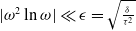 $|\omega ^2\ln \omega |\ll \epsilon =\sqrt {\frac {\delta }{\tau ^2}}$
, one has
 \begin{align*} \xi _1=\xi _2=\mathcal{O}\left (\frac {\delta \ln \omega }{\delta \ln \omega }\right )=\mathcal{O}(1) \quad \text{and}\quad \xi _3=\mathcal{O}\left (\frac {\delta \omega }{\delta }\right )=\mathcal{O}(\omega ). \end{align*}
When
 $|\omega ^2\ln \omega |=\mathcal{O}(\epsilon )$
, one has
 \begin{align*} \xi _1=\xi _2&=\mathcal{O}\left (\frac {\delta \ln \omega }{\omega ^2 \ln \omega }\right )=\mathcal{O}(|\ln \omega |) \quad \text{and}\quad \xi _3=\mathcal{O}\left (\frac {|\omega ^3\ln \omega |}{\delta }\right )=\mathcal{O}(\omega ). \end{align*}
When
 $\omega ^2\ll \epsilon \ll |\omega ^2\ln \omega |\ll 1$
, one has
 \begin{equation*}\mathcal{O}\left (\frac {1}{|\omega \ln \omega |}\right )\ll \xi _1=\xi _2=\mathcal{O}\left (\frac {\delta |\ln \omega |}{|\omega ^2\ln ^2 \omega |}\right )=\mathcal{O}\left (\frac {\delta }{|\omega ^2\ln \omega |}\right )\ll \mathcal{O}(1),\end{equation*}
and
 \begin{equation*} \mathcal{O}(\omega ) \ll \xi _3 = \mathcal{O}\left (\frac {|\omega ^3\ln \omega |}{\delta }\right ) \ll \mathcal{O}(\omega |\ln \omega |). \end{equation*}
When
 $\omega ^2=\mathcal{O}(\epsilon )$
, one has
 \begin{align*} \xi _1=\xi _2=\mathcal{O}\left (\frac {|\delta \ln \omega |}{\omega ^2\ln ^2\omega }\right )=\mathcal{O}\left (\frac {1}{|\ln \omega |}\right )\quad \text{and}\quad \xi _3=\mathcal{O}\left (\frac {|\omega ^3\ln \omega |}{\omega ^4\ln ^2\omega }\right )=\mathcal{O}\left (\frac {1}{|\omega \ln \omega |}\right )\!. \end{align*}
When
 $\epsilon \ll \omega ^2\ll 1$
, one has
 \begin{align*} \xi _1=\xi _2=\mathcal{O}\left (\frac {|\delta \ln \omega |}{\omega ^2 \ln ^2\omega }\right )=\mathcal{O}\left (\frac {\delta }{|\omega ^2\ln \omega |}\right ) \quad \text{and}\quad \xi _3=\mathcal{O}\left (\frac {|\omega ^3\ln \omega |}{\omega ^2}\right )=\mathcal{O}(\omega |\ln \omega |). \end{align*}
We complete the proof.
4.2. Far-field patterns
This section focuses on the far-field patterns of the scattered field in the exterior domain, including both longitudinal (denoted by
 $\boldsymbol{u}_{p,\infty }(\hat {\boldsymbol x})$
) and transverse (denoted by
 $\boldsymbol{u}_{s,\infty }(\hat {\boldsymbol x})$
) far-field patterns. Here,
 $\hat {\boldsymbol x}=\frac {\boldsymbol x}{|\boldsymbol x|}$
. Clearly, these far-field patterns are defined on the unit circle in
 $\mathbb{R}^2$
. We begin by presenting an important property related to the Kupradze matrix
 $\boldsymbol{G}^{k}(\boldsymbol x-\boldsymbol y)$
, as detailed in [Reference Sevroglou31].
Lemma 4.4.
As
 $|\boldsymbol x|\rightarrow +\infty$
and
 $k\rightarrow 0$
, it holds for
 $\boldsymbol{y}\in \partial D$
that
 \begin{align*} \boldsymbol{G}^{k}(\boldsymbol{x}-\boldsymbol{y}) = &-\frac {\mathrm{i}+1}{4(\lambda +2\mu )^{3/4}\sqrt {\pi k}} \, \widehat {\boldsymbol{x}}\widehat {\boldsymbol{x}}^\top \, e^{-\mathrm{i} \frac {k}{\sqrt {\lambda +2\mu }}\widehat {\boldsymbol{x}}\cdot \boldsymbol{y}} \, \frac {e^{\mathrm{i}\frac {k}{\sqrt {\lambda +2\mu }}|\boldsymbol{x}|}}{\sqrt {|\boldsymbol{x}|}} \\[2pt] &-\frac {\mathrm{i}+1}{4\mu ^{3/4}\sqrt {\pi k}} \, (\mathbf{I}-\widehat {\boldsymbol{x}}\widehat {\boldsymbol{x}}^\top ) \, e^{-\mathrm{i} \frac {k}{\sqrt {\mu }}\widehat {\boldsymbol{x}}\cdot \boldsymbol{y}} \, \frac {e^{\mathrm{i}\frac {k}{\sqrt {\mu }}|\boldsymbol{x}|}}{\sqrt {|\boldsymbol{x}|}} + \mathcal{O}\left (|\boldsymbol{x}|^{-3/2}\right ) \end{align*}
uniformly with respect to
 $\hat {\boldsymbol x}$
.
From Lemma 4.4, we directly obtain the corresponding expansion for the specific wavenumber
 $k = \sqrt {\rho }\omega$
:
 \begin{align} \boldsymbol{G}^{\sqrt {\rho }\omega }(\boldsymbol{x}-\boldsymbol{y}) = &-\frac {\mathrm{i}+1}{4\rho ^{1/4}\mu ^{3/4}\sqrt {\pi \omega }} \, (\mathbf{I}-\widehat {\boldsymbol{x}}\widehat {\boldsymbol{x}}^\top ) \, \frac {e^{\mathrm{i}\frac {\sqrt {\rho }\omega }{\sqrt {\mu }}|\boldsymbol{x}|}}{\sqrt {|\boldsymbol{x}|}} \, \left (1+\mathcal{O}(\omega )\right ) \nonumber \\[2pt] &-\frac {\mathrm{i}+1}{4\rho ^{1/4}(\lambda +2\mu )^{3/4}\sqrt {\pi \omega }} \, \widehat {\boldsymbol{x}}\widehat {\boldsymbol{x}}^\top \, \frac {e^{\mathrm{i}\frac {\sqrt {\rho }\omega }{\sqrt {\lambda +2\mu }}|\boldsymbol{x}|}}{\sqrt {|\boldsymbol{x}|}} \, \left (1+\mathcal{O}(\omega )\right ) + \mathcal{O}\left (|\boldsymbol{x}|^{-3/2}\right )\!. \end{align}
Theorem 4.5.
Let
 $D$
be a disk of radius
 $R$
. As
 $\omega ,\delta ,\epsilon \in \mathbb{R}^+\rightarrow 0^+$
, the solution
 $\boldsymbol u_{\mathbb{R}^2\backslash D}$
to (2.7) in the far field admits the expansion:
 \begin{align} \boldsymbol u_{\mathbb{R}^2\backslash D}-\boldsymbol{u}^{\mathrm{in}}(\boldsymbol x)&=\boldsymbol{u}_{p,\infty }(\widehat {\boldsymbol x})\frac {e^{\mathrm{i}\frac {\sqrt {\rho }\omega }{\sqrt {\lambda +2\mu }}|\boldsymbol x|}}{\sqrt {|\boldsymbol x|}}+\boldsymbol{u}_{s,\infty }(\widehat {\boldsymbol x})\frac {e^{\mathrm{i}\frac {\sqrt {\rho }\omega }{\sqrt {\mu }}|\boldsymbol x|}}{\sqrt {|\boldsymbol x|}}+\mathcal{O}\big(\zeta _i|\boldsymbol x|^{-\frac {3}{2}}\big), \end{align}
where
 \begin{align*} \boldsymbol{u}_{p,\infty }(\widehat {\boldsymbol x})\,:\!=\,-\frac {\mathrm{i}+1}{4\rho ^{\frac {1}{4}}(\lambda +2\mu )^{\frac {3}{4}}\sqrt {\pi \omega }}\widehat {\boldsymbol x}\widehat {\boldsymbol x}^\top \sum ^2_{i=1}\zeta _i\,\boldsymbol f^{(i)}\left (1+\mathcal{O}(\omega )\right )+\mathcal{O}\big(\omega ^{\frac {1}{2}}+\delta \omega ^{-\frac {1}{2}}\big), \end{align*}
and
 \begin{align*} \boldsymbol{u}_{s,\infty }(\widehat {\boldsymbol x})&\,:\!=\,-\frac {\mathrm{i}+1}{4\rho ^{\frac {1}{4}}\mu ^{\frac {3}{4}}\sqrt {\pi \omega }}(\mathbf{I}-\widehat {\boldsymbol x}\widehat {\boldsymbol x}^\top ) \sum ^2_{i=1}\zeta _i\,\boldsymbol f^{(i)}\left (1+\mathcal{O}(\omega )\right )+\mathcal{O}\big(\omega ^{\frac {1}{2}}+\delta \omega ^{-\frac {1}{2}}\big). \end{align*}
Here, the magnitudes
 $\zeta _i (i=1,2)$
are characterised by
 \begin{align} \zeta _i=\left \{ {\begin{array}{lll}\mathcal{O}\left (\frac {|\omega ^2\ln \omega |}{\delta }\right )\!,&& |\omega ^2\ln \omega |\ll \epsilon ,\\[2pt] \mathcal{O}(|\ln \omega |),&& |\omega ^2\ln \omega |=\mathcal{O}(\epsilon ),\\ \mathcal{O}(1),&&\omega ^2 \ll \epsilon \ll |\omega ^2\ln \omega | \ll 1,\\ \mathcal{O}(1),&& \omega ^2 = \mathcal{O}(\epsilon ),\\ \mathcal{O}(1),&& \epsilon \ll \omega ^2 \ll 1. \end{array}}\right . \end{align}
Proof. Based on (4.6) and (4.10), we derive the expression:
 \begin{align} \boldsymbol u_{\mathbb{R}^2\backslash D}-\boldsymbol u^{\mathrm{in}} & = \widetilde {\boldsymbol{\mathcal{S}}}_D^{\sqrt {\rho }\omega }\left [\sum ^3_{i=1}\alpha _ib_ia_i\,\boldsymbol f^{(i)}+\sum ^2_{i=1}\tilde {\eta }d_i\,\boldsymbol f^{(i)}+\mathcal{\mathcal{O}}(\omega +\delta )\right ]\nonumber \\[3pt] & = \int _{\partial D}\boldsymbol{G}^{\sqrt {\rho }\omega }(\boldsymbol x-\boldsymbol y)\left (\sum ^3_{i=1}\alpha _ib_ia_i\,\boldsymbol f^{(i)}+\sum ^2_{i=1}{\tilde {\eta } d_i}\,\boldsymbol f^{(i)}+\mathcal{O}(\omega +\delta )\right )\mathrm{d}\sigma (\kern1pt\boldsymbol y). \end{align}
Set
 \begin{align*} \zeta _i=2\pi R(\alpha _ib_ia_i+{\tilde {\eta } d_i}), \quad \text{for } i=1,2. \end{align*}
Combining (4.12), (4.15) and (3.17), we get (4.13). Moreover, combining (4.4) and (4.8), we obtain for
 $i=1,2$
that
 \begin{align*} & \omega ^2 \ln \omega \, \rho \tau ^2 (\alpha _i b_i + \eta d_i) Q_{ii} + \omega ^2 \rho \tau ^2 \ln (\sqrt {\rho }\tau ) (\alpha _i b_i + \eta d_i) Q_{ii} \\ &\quad + \omega ^2 \rho \tau ^2 (\alpha _i b_i + \eta d_i) P_{ii} \mathcal{O}(\delta \omega ^2 \ln \omega + \omega ^4 \ln \omega + \omega ^4) \\ & = \delta d_i\left (\alpha _ib_ia_i+\tilde {\eta }d_i\right ) + \mathcal{O}(\omega ^3 \ln \omega + \omega ^3 + \omega \delta ). \end{align*}
5. Dilute phononic structure
When resonators are arranged periodically, the subwavelength bandgap exists in two-dimensional phononic crystals, as established in [Reference Ren, Chen, Gao and Li30]. This section extends this analysis to the dilute structure, where the distance between adjacent resonators is significantly larger than the size of an individual resonator, as illustrated in Figure 1.
Two-dimensional phononic crystal with a dilute structure.

Let
 $\Omega =s D$
with the scaling factor
 $0\lt s\ll 1$
, where
 $D$
denotes a disk of radius
 $R$
. Moreover, assume
 $|\frac {\epsilon }{s^2\ln s}|\ll 1$
. For the quasi-momentum variable
 $\boldsymbol \alpha \in [{-}\pi ,\pi ]^2\backslash \boldsymbol{0}$
, define the quasi-periodic single-layer potential
 $\boldsymbol{\mathcal{S}}^{\boldsymbol{\alpha },0}_{\Omega }\,:\, L^{2}(\partial \Omega )^2\rightarrow H^{1}(\partial \Omega )^2$
as
 \begin{align*} \boldsymbol{\mathcal{S}}^{\boldsymbol{\alpha },0}_{\Omega }[\boldsymbol \varphi ](\boldsymbol x)\,:\!=\,\int _{\partial \Omega }\boldsymbol{G}^{\boldsymbol{\alpha },0}(\boldsymbol x-\boldsymbol y)\boldsymbol \varphi (\kern1pt\boldsymbol y)\mathrm{d}\sigma (\kern1pt\boldsymbol y),\quad \boldsymbol x\in \partial \Omega , \end{align*}
where the quasi-periodic fundamental solution:
 \begin{align*} \boldsymbol{G}^{\boldsymbol{\alpha },0}(\boldsymbol x-\boldsymbol y)=\sum _{\boldsymbol{n}\in \mathbb{Z}^{2}}\boldsymbol{G}^{0}(\boldsymbol x-\boldsymbol y-\boldsymbol{n})e^{\mathrm{i}\boldsymbol{n}\cdot \boldsymbol \alpha } \end{align*}
with
 $\boldsymbol{G}^{0}(\boldsymbol x)=(G_{ij}^{0}(\boldsymbol x))^2_{i,j=1}$
defined by (2.8). Then, the following lemma can be formulated, with its proof available in Theorem 3.14 of [Reference Ren, Chen, Gao and Li30].
Lemma 5.1.
For the phononic crystals constructed from the periodic arrangement of resonator
 $\Omega$
, there exists a subwavelength bandgap above the frequency:
 \begin{align} \omega ^{\boldsymbol \alpha }_{\ast }\,:\!=\,\max _{i=1,2}\max _{\boldsymbol \alpha \in [-\pi ,\pi ]^2\backslash \boldsymbol 0}\sqrt {\frac {\lambda ^{\boldsymbol \alpha }_i}{\rho |\Omega |}}\epsilon ^{\frac {1}{2}}, \end{align}
where
 $\lambda ^{\boldsymbol \alpha }_i(i=1,2)$
are the eigenvalues of the matrix:
 \begin{align} \boldsymbol{Q^\alpha }\,:\!=\,(Q^{\boldsymbol \alpha }_{ij})^2_{i,j=1}\quad \text{with} \quad Q^{\boldsymbol \alpha }_{ij}=-\int _{\partial \Omega } (\boldsymbol{\mathcal{S}}^{\boldsymbol \alpha ,0}_\Omega )^{-1}[\boldsymbol e_i](\boldsymbol x)\cdot \boldsymbol e_j\mathrm{d}\sigma (\boldsymbol x). \end{align}
Here,
 $\boldsymbol{e}_i(i=1,2)$
denote the standard unit vectors in
 $\mathbb{R}^2$
.
In dilute case, the following theorem further characterises the frequency
 $\omega ^{\boldsymbol \alpha }_{\ast }$
defined in (5.1).
Theorem 5.2.
Let
 $D$
be a disk of radius
 $R$
and let
 $\Omega =sD$
with a scaling factor
 $0\lt s\ll 1$
such that
 $|\frac {\epsilon }{s^2\ln s}|\ll 1$
. For
 $|\boldsymbol \alpha |\gt c\gt 0$
, there exist a subwavelength phononic bandgap slightly above the frequency:
 \begin{align*} \omega _{\ast }=\operatorname {Re}\sqrt {\frac {-2t\epsilon }{\rho R s^2}}, \end{align*}
where
 \begin{align} t=\frac {1}{\tau _1 R\ln R-\frac {\tau _2}{2} R+2\pi R\beta _{s}} \end{align}
with
 $\tau _1,\tau _2$
given by (2.10) and
 $\beta _{s}$
given by (2.11).
Proof. Define the matrix-valued function:
 \begin{align*} \boldsymbol \Lambda ^{\boldsymbol \alpha }=\big(\Lambda ^{\boldsymbol \alpha }_{ij}\big)^2_{i,j=1} \quad \text{with}\quad \Lambda ^{\boldsymbol \alpha }_{ij}(\boldsymbol x)=G^{\boldsymbol \alpha ,0}_{ij}(\boldsymbol x)-G^{0}_{ij}(\boldsymbol x). \end{align*}
Note that
 $\boldsymbol \Lambda ^{\boldsymbol \alpha }(\boldsymbol x)$
is smooth and admits the expansion:
 \begin{equation*}\boldsymbol \Lambda ^{\boldsymbol \alpha }(\boldsymbol x)=\boldsymbol \Lambda ^{\boldsymbol \alpha }(0)+\mathcal{O}(|\boldsymbol x|), \quad \mathrm{\,as\,}|\boldsymbol x|\to 0.\end{equation*}
Let
 $\boldsymbol x,\boldsymbol y\in \partial D$
, so that
 $s\boldsymbol x, s\boldsymbol y\in \partial \Omega$
. It follows for
 $\boldsymbol \varphi \in L^{2}(\partial \Omega )^2$
that
 \begin{align} \boldsymbol{\mathcal{S}}^{\boldsymbol \alpha ,0}_{\Omega }[\boldsymbol \varphi ](s \boldsymbol x)=&\,s\int _{\partial D}\boldsymbol G^{\boldsymbol \alpha ,0}(s \boldsymbol x-s \boldsymbol y)\boldsymbol \varphi (s \boldsymbol y)\mathrm{d}\sigma (\kern1pt\boldsymbol y)\nonumber \\[2pt] =&\,s\int _{\partial D}\boldsymbol G^{0}(\boldsymbol x-\boldsymbol y)\widetilde {\boldsymbol \varphi }(\kern1pt\boldsymbol y)\mathrm{d}\sigma (\kern1pt\boldsymbol y) +s\ln s\frac {\lambda +3\mu }{4\pi \mu (\lambda +2\mu )}\int _{\partial D}\widetilde {\boldsymbol \varphi }(\kern1pt\boldsymbol y)\mathrm{d}\sigma (\kern1pt\boldsymbol y)\nonumber \\[2pt] &+s\int _{\partial D}\boldsymbol{\Lambda }^{\boldsymbol \alpha }(0)\widetilde {\boldsymbol \varphi }(\kern1pt\boldsymbol y)\mathrm{d}\sigma (\kern1pt\boldsymbol y) +s\int _{\partial D}\mathcal{O}(s|\boldsymbol x-\boldsymbol y|)\widetilde {\boldsymbol \varphi }(\kern1pt\boldsymbol y)\mathrm{d}\sigma (\kern1pt\boldsymbol y)\nonumber \\[2pt] =&\,s\hat {\boldsymbol{\mathcal{S}}}^{s}_D[\widetilde {\boldsymbol \varphi }](\boldsymbol x)+s\left ({\ln}\, s\frac {\lambda +3\mu }{4\pi \mu (\lambda +2\mu )}-\beta _s\right )\int _{\partial D}\widetilde {\boldsymbol \varphi }(\kern1pt\boldsymbol y)\mathrm{d}\sigma (\kern1pt\boldsymbol y)\nonumber \\[2pt] &\,+s\boldsymbol{\Lambda }^{\boldsymbol \alpha }(0)\int _{\partial D}\widetilde {\boldsymbol \varphi }(\kern1pt\boldsymbol y)\mathrm{d}\sigma (\kern1pt\boldsymbol y)+\mathcal{O}(s^2)\nonumber \\[2pt] =&\,s\hat {\boldsymbol{\mathcal{S}}}^{s}_D\big(\boldsymbol{\mathcal{I}}-\big(\hat {\boldsymbol{\mathcal{S}}}^{s}_D\big)^{-1}\boldsymbol{\Pi }\big)[\widetilde {\boldsymbol \varphi }](\boldsymbol x), \end{align}
where
 $\widetilde {\boldsymbol \varphi }(\boldsymbol x)=\boldsymbol \varphi (s \boldsymbol x)$
and
 \begin{align*} \boldsymbol{\Pi }[\widetilde {\boldsymbol \varphi }]=\int _{\partial D}\left (\left (\frac {\tau _1}{4\pi }(2\gamma - \pi \mathrm{i} - \ln 4) + \frac {\tau _2}{4\pi } - \frac {\ln (\lambda +2\mu )}{8\pi (\lambda + 2\mu )} -\frac {\ln \mu }{8\pi \mu }\right )\boldsymbol{I}-\boldsymbol \Lambda ^{\boldsymbol \alpha }(0)\right )\widetilde {\boldsymbol \varphi }(\kern1pt\boldsymbol y)\mathrm{d}\sigma (\kern1pt\boldsymbol y) \end{align*}
for
 $\widetilde {\boldsymbol \varphi }\in L^{2}(\partial D)^2$
. Given that
 $\hat {\boldsymbol{\mathcal{S}}}^{s}_D$
involves
 $\ln s$
and
 $|\ln s|\rightarrow +\infty$
as
 $s\rightarrow 0$
, we can obtain
 \begin{align*} \big\|\big(\hat {\boldsymbol{\mathcal{S}}}^{s}_D\big)^{-1}\boldsymbol{\Pi }\big\|_{\mathcal{L}(L^{2}(\partial D)^2,L^{2}(\partial D)^2)}\lt 1, \end{align*}
where
 $\mathcal{L}(L^{2}(\partial D)^2,L^{2}(\partial D)^2)$
denotes the space of bounded linear operators from
 $L^{2}(\partial D)^2$
to
 $L^{2}(\partial D)^2$
. Then, (5.4) indicates that
 \begin{align} \big(\boldsymbol{\mathcal{S}}^{\boldsymbol \alpha ,0}_{\Omega }\big)^{-1}[\boldsymbol e_i]= s^{-1}\big(\hat {\boldsymbol{\mathcal{S}}}^{s}_D\big)^{-1}[\boldsymbol e_i]+O(s^{-1}\ln ^{-2} s). \end{align}
We now focus on computing
 $(\hat {\boldsymbol{\mathcal{S}}}^{s}_D)^{-1}[\boldsymbol e_i]$
. Assume
 $\widetilde {\boldsymbol \varphi }(\boldsymbol x)\in L^{2}(\partial D)^2$
satisfying
 $\hat {\boldsymbol{\mathcal{S}}}^{s}_D[\widetilde {\boldsymbol \varphi }]=\boldsymbol e_i.$
One has
 \begin{align*} \boldsymbol{\mathcal{S}}_D[\widetilde {\boldsymbol \varphi }]+\beta _s\int _{\partial D}\widetilde {\boldsymbol \varphi }(\kern1pt\boldsymbol y)\mathrm{d}\sigma (\kern1pt\boldsymbol y)=\boldsymbol e_i. \end{align*}
According to
 $(\mathrm{i})$
and
 $(\mathrm{ii})$
in Lemma 2.4, it holds that
 $\widetilde {\boldsymbol \varphi }=t\boldsymbol e_i$
with a constant
 $t$
. Then, we obtain
 \begin{align*} \left (\tau _1 R\ln R-\frac {\tau _2}{2} R\right )t\boldsymbol e_i+2\pi R\beta _st\boldsymbol e_i=\boldsymbol e_i, \end{align*}
which indicates (5.3). It holds from (5.2) and (5.5) that
 \begin{align} Q^{\boldsymbol \alpha }_{ij}&=-\int _{\partial \Omega }s^{-1} \big(\hat {\boldsymbol{\mathcal{S}}}^s_D\big)^{-1}[\boldsymbol e_i](\boldsymbol x)\cdot \boldsymbol e_j\mathrm{d}\sigma (\boldsymbol x)+\mathcal{O}({\ln}^{-2}s)\nonumber \\ &=-\operatorname {Re}2\pi Rt\delta _{ij}+\mathcal{O}({\ln} ^{-2}s).\end{align}
In the above expression, the last equality utilises
 $\operatorname {Re} t=\mathcal{O}(|\ln ^{-1}s|)$
and
 $\operatorname {Im} t=\mathcal{O}({\ln} ^{-2}s)$
. Note that
 $\operatorname {Re} t \lt 0$
as
 $s \to 0$
. Then, it follows that
 $\operatorname {Re} \sqrt {\frac {-2t \epsilon }{\rho R s^2}} \gt 0$
, which is consistent with the fact that the eigenvalues of the matrix
 $\mathbf{Q}^\alpha$
are positive real numbers (see Lemma 3.11 in [Reference Ren, Chen, Gao and Li30]). Combining (5.1) with (5.6) yields
 \begin{align*} \omega ^{\boldsymbol \alpha }_{\ast }=\operatorname {Re}\sqrt {\frac {-2\pi Rt\epsilon }{\rho |\Omega |}}+\mathcal{O}\left (\sqrt {\frac {\epsilon }{s^2\ln ^2s}}\right )=\operatorname {Re}\sqrt {\frac {-2t\epsilon }{\rho R s^2}}+\mathcal{O}\left (\sqrt {\frac {\epsilon }{s^2\ln ^2s}}\right )\!. \end{align*}
Therefore, by Lemma 5.1, the proof is complete.
6. Concluding remarks
This paper presents a systematic analysis of wave scattering by a hard elastic inclusion embedded in a soft elastic matrix in two-dimensional space using layer potential techniques. By examining the spectral properties of the associated boundary integral operators, we characterise the asymptotic behaviours of subwavelength resonant frequencies. Furthermore, we describe the scattering fields both inside and outside the resonator across various regimes of incident frequencies. Finally, extending the result of [Reference Ren, Chen, Gao and Li30], we determine the location of the subwavelength bandgap in dilute elastic phononic crystals.
As noted in Section 1, our current analysis is limited to radial configurations due to the specific asymptotic expansion of the two-dimensional fundamental solution and the spectral properties of the boundary integral operators. Generalising these results to arbitrary geometries will be the subject of future research. We are also particularly interested in developing an effective medium theory for randomly distributed elastic particles. Such a system represents a non-periodic configuration.
Acknowledgements
The authors thank the anonymous reviewers and the editorial team for their constructive comments and suggestions, which have greatly strengthened this work. The authors specially thank Professor Peijun Li for his insightful discussions and valuable advice.
Funding statement
The work of YG was supported by NSFC grants (project numbers, 12371187 and 12071065) and Science and Technology Development Plan Project of Jilin Province (project number, 20240101006JJ).
Competing interests
The authors declare no competing interests.
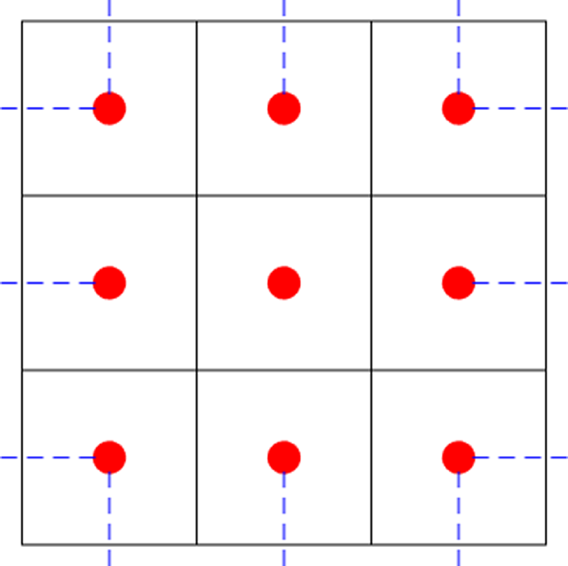

 Open access

