


1. Introduction
Humans exhibit diverse reproductive strategies, as can be observed by comparing fertility rates both between (Davison and Gurven, Reference Davison and Gurven2021) and within populations (Ross et al., Reference Ross, Hooper, Smith, Jaeggi, Smith, Gavrilets, Zohora, Ziker, Xygalatas and Wroblewski2023). The observed diversity in completed fertility has been largely associated with differences in the amount of resources available, usually proxied for by material wealth ownership or access (Low et al., Reference Low, Hazel, Parker and Welch2008, Stulp et al., Reference Stulp, Sear, Schaffnit, Mills and Barrett2016, Uggla and Mace, Reference Uggla and Mace2016, Fieder and Huber, Reference Fieder and Huber2022). Life history theory predicts that under many conditions, favourable resource access will hasten the age at which females first give birth. However, in long-lived species, especially those with extended juvenile dependence and skill-intensive diets, individuals with greater access to resources should start their reproductive careers later in life (see Kaplan (Reference Kaplan1996) for the case in humans, Fay et al. (Reference Fay, Barbraud, Delord and Weimerskirch2016) for foraging seabirds, and Stearns and Crandall (Reference Stearns and Crandall1981) more generally). Wealth can be accumulated by delaying reproductive onset, and this wealth can then be allocated towards parental care (‘quantity versus quality of offspring’ trade-off) and/or higher amounts of embodied capital (‘somatic versus reproductive investment’ trade-off) (Lack, Reference Lack1947, Kaplan, Reference Kaplan1996). However, despite evidence of a negative relationship between wealth and fertility in early research on the topic (Vining Jr, Reference Vining1986), observed wealth–fertility associations in high-income countries with high-quality longitudinal data tend to be positive (Stulp and Barrett, Reference Stulp and Barrett2016). More generally, wealth–fertility relationships are highly variable across contexts: for example, positive associations have been observed among the Kipsigis in Kenya (Borgerhoff Mulder, Reference Borgerhoff Mulder1989a) and negative ones among Chilean women (Varas Enríquez et al., Reference Varas Enríquez, McKerracher and Montalva Rivera2022). In addition, the relationship between wealth and fertility seems to vary depending on which aspect of resource availability is measured (e.g., wealth versus status (Colleran et al., Reference Colleran, Jasienska, Nenko, Galbarczyk and Mace2015)), the nature of the data analysed (e.g., cross-sectional versus longitudinal data (Kolk, Reference Kolk2023)), and/or the production system of societies (Page et al., Reference Page, Ringen, Koster, Borgerhoff Mulder, Kramer, Shenk, Stieglitz, Starkweather, Ziker and Boyette2024). Our primary goal here is to explore the complexities behind the varied patterning of the relationship between resource availability and the reproductive strategies of women, using longitudinal data collected in a non-Western population of indigenous Pimbwe people in Tanzania.
We focus on age at first birth, a crucial life history trait, due to its influence on the length of the reproductive career of women and their subsequent fitness (Käär et al., Reference Käär, Jokela, Helle and Kojola1996, Kirk et al., Reference Kirk, Blomberg, Duffy, Heath, Owens and Martin2001, Byars et al., Reference Byars, Ewbank, Govindaraju and Stearns2010, Stearns et al., Reference Stearns, Byars, Govindaraju and Ewbank2010). Age at first birth is a highly variable trait, which is biologically constrained by age at menarche (from  $10$ years old) and menopause (to
 $60$ years old) (Thomas et al., Reference Thomas, Renaud, Benefice, De Meeüs and Guegan2001, Wood, Reference Wood2017). Across multiple countries, the average age at first birth is
 $26.84$ years old, with a standard deviation (SD) of
 $3.42$ (Bulley and Pepper, Reference Bulley and Pepper2017). There is a wide range in average age at first birth among countries (
 $\sim18$ to
 $\sim31$ years old) (Low et al., Reference Low, Hazel, Parker and Welch2008) and also among small-scale populations (
 $\sim 16.2$ to
 $\sim 25.7$ years old) (Walker et al., Reference Walker, Gurven, Hill, Migliano, Chagnon, De Souza, Djurovic, Hames, Hurtado and Kaplan2006). Within populations, age at first birth can also be highly variable. In post-demographic transition England, the average age at first birth is
 $28.59$ years old (SD
 $=5.93$) (Nettle, Reference Nettle2010), in mid-demographic transition Chile the average age at first birth is
 $22.54$ years old (SD
 $=5.06$) (Varas Enríquez et al., Reference Varas Enríquez, McKerracher and Montalva Rivera2022), whereas in the pre-demographic transition Agta, the average at first birth is
 $20.14$ years old (SD
 $=2.97$) (Goodman et al., Reference Goodman, Estioko-Griffin, Griffin and Grove1985). The sources of variation in the ages at first birth among and within populations appear to involve a complex interplay of different social and environmental factors.
Both theory and empirical work suggest that starting to reproduce early can increase the number of lifetime reproductive opportunities, but can simultaneously reduce the survival probabilities of both the mother and her child, due to ‘maternal depletion’ (Hurtado and Hill, Reference Hurtado and Hill1996, Tracer, Reference Tracer2002, Allal et al., Reference Allal, Sear, Prentice and Mace2004, Nenko and Jasienska, Reference Nenko and Jasienska2009, Kramer and Lancaster, Reference Kramer and Lancaster2010, Liu and Lummaa, Reference Liu and Lummaa2011, Perez-Alvarez and Favara, Reference Perez-Alvarez and Favara2023). On the other hand, a woman who begins to reproduce later can accumulate more resources for subsequent investment in either her own embodied capital or in the ‘quality’ of her descendants, rather than in having more children. Such life history trade-offs are referred to, respectively, as the ‘somatic versus reproductive investment’ and ‘quantity versus quality of offspring’ trade-offs, both of which are responsive to resource availability (Figure 1a) (Kaplan, Reference Kaplan1996, Hill and Kaplan, Reference Hill and Kaplan1999, Snopkowski and Kaplan, Reference Snopkowski and Kaplan2014).
Summary of expected relationships between the probability of first birth (Prob. (FB)) and absolute wealth (a. $1$–
 $4$) and variability in wealth (b.
 $1$–
 $4$), based on the different hypotheses. The differences are displayed in terms of the minimum (Min.), medium (Med.), and maximum (Max.) levels of absolute wealth and its variability. Regarding absolute wealth, life history trade-offs between both the quantity and quality of offspring and the need to invest in somatic versus reproductive effort generally predict a late reproductive onset of women with higher amounts of wealth. In terms of wealth variability, the prediction is that women who experience more variability will start their reproductive career early, as a result of responding to environmental uncertainty and/or the life history trade-offs between current and future reproduction. These predictions can be seen in the overall differences among the curves (a.1, b.1), the median age at first birth (a.2, b.2), the modal age at first birth (a.3, b.3), and the age at maximum differences (a.4, b.4). The modal age at first birth refers to the age interval with the largest change in the cumulative probability of first birth in response to a wealth predictor. The age at maximum difference refers to the age at which the difference in cumulative probability of first birth is largest for each pair of wealth predictor levels.

Figure 1 Long description
Multi-line graphs comparing the probability of first birth with absolute wealth and wealth variability across different ages. The horizontal axis represents age, while the vertical axis represents the probability of first birth (Prob. (FB)). Each graph displays three curves representing minimum (Min.), medium (Med.) and maximum (Max.) levels of wealth or wealth variability. Absolute Wealth (Graphs a.1 to a.4): - Graph a.1 shows overall differences, with higher wealth leading to later first births. The Min. line is left-shifted, indicating earlier births compared to Med. and Max. - Graph a.2 highlights median age at first birth, showing earlier median ages for Min. wealth. - Graph a.3 depicts modal age at first birth, with Min. wealth having the earliest mode. - Graph a.4 shows age at maximum differences, where Min. wealth results in the earliest significant change. Wealth Variability (Graphs b.1 to b.4): - Graph b.1 shows overall differences, with higher variability leading to earlier first births. The Max. line is right-shifted, indicating later births compared to Min. and Med. - Graph b.2 highlights median age at first birth, showing later median ages for Max. variability. - Graph b.3 depicts modal age at first birth, with Max. variability having the latest mode. - Graph b.4 shows age at maximum differences, where Max. variability results in the latest significant change. The graphs use dashed and dotted lines to mark median, mode and maximum differences, with highlighted segments indicating key age ranges where probability rises steeply. The legend indicates the color coding for Min., Med. and Max. levels.
Empirical evidence suggests that, across contemporary populations, women with higher resource availability typically delay their first births (Low et al., Reference Low, Hazel, Parker and Welch2008, Stulp et al., Reference Stulp, Sear, Schaffnit, Mills and Barrett2016, Uggla and Mace, Reference Uggla and Mace2016, Fieder and Huber, Reference Fieder and Huber2022). This postponement appears to reflect the opportunity for well-resourced women to further invest in human capital, such as education (Adu Boahen, Reference Adu Boahen2024). However, when such opportunities to invest in embodied capital are low (e.g., limited access to schools), absolute wealth tends to be associated with earlier reproduction (Borgerhoff Mulder, Reference Borgerhoff Mulder1989a, Reference Borgerhoff Mulder1989b). Recent evidence in populations from the Global North also shows that high-income women begin reproducing earlier (Van Wijk and Billari, Reference Van Wijk and Billari2024). The influence of resource availability on age at first birth is not well understood, as suggested by the inconsistency of existing findings.
Variation in the availability of resources over time, specifically fluctuations and uncertainty in the amount of resources available to a woman, will also influence age at first birth. This logic is usually presented in life history theory as a trade-off between ‘current versus future reproduction’, wherein earlier reproductive onset under conditions of high resource variability would result in higher reproductive success of women (Figure 1b and in Hill and Kaplan ( Reference Hill and Kaplan1999), Griskevicius et al. ( Reference Griskevicius, Delton, Robertson and Tybur2011); see also the ‘variance compensation hypothesis’ (Leslie and Winterhalder, Reference Leslie and Winterhalder2002, Winterhalder and Leslie, Reference Winterhalder and Leslie2002)). Such theoretical claims are supported by empirical evidence that women who experience greater environmental uncertainty throughout their lives – in terms of wealth and mortality risk – tend to begin reproducing earlier (Low et al., Reference Low, Hazel, Parker and Welch2008, Griskevicius et al., Reference Griskevicius, Delton, Robertson and Tybur2011, Uggla and Mace, Reference Uggla and Mace2016). However, such patterns are by no means consistent. For example, a study comparing populations within Latin America showed that women postpone their reproductive onset in response to high short-term unemployment rates, but hasten their reproductive onset if the unemployment rate is calculated with a 4-year lag (Adsera and Menendez, Reference Adsera and Menendez2011).
Few studies have examined the influence of material wealth and its variability on age at first birth together. In a study of post-demographic transition populations of the Global North, Van Wijk and Billari (Reference Van Wijk and Billari2024) found the income of women to be positively associated with age at first birth, although their perceptions of economic uncertainty played no major role. In another example focusing on the interaction between economic uncertainty and socioeconomic status during childhood conducted among undergraduate students in Singapore, Tan et al. (Reference Tan, Li, Meltzer, Chin, Tan, Lim, Neuberg and van Vugt2022) found that cues of economic uncertainty were associated with preferences for earlier first births, but only among students from lower socioeconomic backgrounds. Uggla and Mace (Reference Uggla and Mace2016) combined population-level indicators of environmental uncertainty with individual-level measures of wealth, and found that only poorer women in post-demographic transition Northern Ireland respond to uncertainties by beginning to reproduce earlier. These findings contrast with those of Low et al. (Reference Low, Hazel, Parker and Welch2008), who showed that, using national-level data of  $\sim 170$ countries, unpredictability accelerates the start of reproduction only in contexts where high wealth promotes delayed childbearing.
Overall, existing empirical research in this area is limited by the difficulty in measuring the value of material wealth, as well as capturing its variability over time. Because wealth is hard to measure, researchers have relied on various proxies to measure wealth at individual (Sheppard et al., Reference Sheppard, Pearce and Sear2016, Varas Enríquez et al., Reference Varas Enríquez, McKerracher and Montalva Rivera2022) and aggregate levels (Low et al., Reference Low, Hazel, Parker and Welch2008, Nettle, Reference Nettle2010), as well as the use of retrospective socioeconomic self-reports (Griskevicius et al., Reference Griskevicius, Delton, Robertson and Tybur2011, Tan et al., Reference Tan, Li, Meltzer, Chin, Tan, Lim, Neuberg and van Vugt2022) or reliance on occupational status (Modena et al., Reference Modena, Rondinelli and Sabatini2014). Similarly, for wealth variability – or environmental uncertainty – researchers have used diverse proxies at the aggregate level (e.g., state-level unemployment rate (Currie and Schwandt, Reference Currie and Schwandt2014), crime rates (Uggla and Mace, Reference Uggla and Mace2016), or country-level life expectancy (Low et al., Reference Low, Hazel, Parker and Welch2008)), whereas for uncertainty at the individual-level researchers have mainly used perceptions regarding job security, economic crises, and environmental safety (Modena et al., Reference Modena, Rondinelli and Sabatini2014, Amir et al., Reference Amir, Jordan and Bribiescas2016, Tan et al., Reference Tan, Li, Meltzer, Chin, Tan, Lim, Neuberg and van Vugt2022). While these proxies are useful, they capture different dimensions of wealth and uncertainty, which could explain the mixed findings in previous studies. In contrast, the use of direct measures at the individual level, and in the period leading up to the age of reproductive onset, may help to clarify the relationship between wealth and the reproductive strategies of women. In short, with a focus on directly observed indicators of material wealth (as pioneered in early work (Hurtado and Hill, Reference Hurtado and Hill1996), and see Sear et al. ( Reference Sear, Lawson, Kaplan and Shenk2016), Stulp and Barrett ( Reference Stulp and Barrett2016), Stulp et al. ( Reference Stulp, Sear, Schaffnit, Mills and Barrett2016)), we propose that individual-level measures of wealth – and their variability over time through a longitudinal approach – may offer a more precise understanding of how material wealth shapes the timing of reproductive onset in women.
In this study, we address limitations to previous research on wealth effects on fertility by using direct, time-varying measures of material wealth as well as short- and long-term measures of wealth variability. To do this, we leverage a longitudinal data set on wealth and fertility measures collected in a primarily Pimbwe community in Tanzania. We analyse the reproductive careers of individual women, linked to direct measures of the material wealth of the households in which they lived before starting their reproductive careers. Our focus is on material wealth because of earlier research highlighting its importance for the survival and well-being of children (Borgerhoff Mulder, Reference Borgerhoff Mulder2009a, Borgerhoff Mulder and Beheim, Reference Borgerhoff Mulder and Beheim2011). More specifically, we explore how material wealth relates to the timing of reproductive onset, and differentiate between the association of absolute wealth and its variability, by focusing on three research questions (Figure 2):
Directed Acyclic Graph (DAG) describing our hypothesised causal relationships between timing of first birth ( $FB_{[i,t]}$) and different wealth predictors. We assume that the three wealth measures, the current amount of wealth in the household of woman
 $i$ at time
 $t$ (
 $W_{[i,t]}$), her short-term variability (
 $\Delta W_{[i,t]}$), and her long-term wealth variability (
 $Var(W)_{[i,t]}$), might make it more or less likely for this woman to have her first birth in this year relative to what is expected for her age. We assume that age (
 $AGE_{[i,t]}$) does not directly cause the first birth of a woman, but its influence is mediated by unmeasured variables associated with biological and social processes affecting fertility (circled
 $U$ in the DAG).

• How do current levels of material wealth relate to the timing of first birth of women?
• How does short- and long-term variability in household material wealth associate with the timing of first birth of women?
• How does the relationship between current levels of material wealth and the timing of first birth of women differ from relationships with short- and long-term wealth variability?
2. Methods
2.1. Population of study
The study village in the Rukwa Valley, now in Katavi (but at the time of study, Rukwa) Region in western Tanzania, is primarily the home of Pimbwe and related ethnic groups of Bantu origin (Seel et al., Reference Seel, Mgawe and Borgerhoff Mulder2014). Pimbwe rely on farming and foraging for subsistence (e.g., cassava production, fishing, and hunting), while increasingly engaging in market-oriented, agricultural activities and livestock raising (e.g., maize, sunflower, rice, and cattle). Items of material wealth are very limited, and mostly not differentiated by gender. For this study, the wealth of young women approaching their first birth is proxied by the items of wealth linked to the household (and the associated farm) where they live (Borgerhoff Mulder, Reference Borgerhoff Mulder2021). The area is characterised by high food insecurity (Hadley et al., Reference Hadley, Borgerhoff Mulder and Fitzherbert2007), unpredictable crop productivity (Borgerhoff Mulder, Reference Borgerhoff Mulder2021), poor child growth (Hadley, Reference Hadley2005), substantial child mortality (Borgerhoff Mulder and Beheim, Reference Borgerhoff Mulder and Beheim2011), high levels of maternal anxiety (Hadley and Patil, Reference Hadley and Patil2008), and rather weak and variable patterns of cooperation among households (Hadley, Reference Hadley2004, Hadley et al., Reference Hadley, Borgerhoff Mulder and Fitzherbert2007, Kasper and Borgerhoff Mulder, Reference Kasper and Borgerhoff Mulder2015). Many of these outcomes are, or are likely to be, associated with variations in material, relational, and somatic wealth (as measured in Borgerhoff Mulder and Beheim (Reference Borgerhoff Mulder and Beheim2011)), making this a suitable context within which to test hypotheses regarding the relationship between material wealth and onset of reproduction. Marriage is usually a very informal affair, with pregnancies occurring either before or after marriage. Couples simply move into a shared new household (Borgerhoff Mulder, Reference Borgerhoff Mulder2009a), although in some cases marriage payments are made and traditional (or religious, most commonly Christian) celebrations are held (Seel et al., Reference Seel, Mgawe and Borgerhoff Mulder2014). Most unions are monogamous. Serial monogamy (for both men and women, following divorce) is very common (Borgerhoff Mulder, Reference Borgerhoff Mulder2009a, Borgerhoff Mulder and Ross, Reference Borgerhoff Mulder and Ross2019), with the result that households, and household membership, are unstable over time (Brockington and Noe, Reference Brockington and Noe2021, Minocher et al., Reference Minocher, Borgerhoff Mulder and Ross2024), with dependents either moving to one of their parent’s new marital home, settling with a grandmother, aunt, or sibling, finding their own partner, or residing alone.
Nowadays young women have considerable, if not complete, autonomy with respect to whom they settle down with and marry, whereas in former times parental control was more prominent but highly variable (Maurice, Reference Maurice1936). Although completed family sizes are large (typically around  $6$ or
 $7$ children, with little evidence of use of family planning (Borgerhoff Mulder, Reference Borgerhoff Mulder2009a)) and no evidence that the population has entered into demographic transition (Borgerhoff Mulder and Ross, Reference Borgerhoff Mulder and Ross2019), there is no prominent pro-natal cultural value, likely because of the widely recognised costs of supporting large families in such a food-insecure environment. Our analyses of the population to date suggest how Pimbwe women appear to adopt strategies such as moving between households or seeking divorce to cope with economic shocks and, in particular, the food insecurity that characterises this population (Hadley et al., Reference Hadley, Borgerhoff Mulder and Fitzherbert2007). These behavioural strategies might lessen the variability of resource availability among women (as we return to in Section 4), though they do not confound the analysis of the association between material wealth and the age at first birth.
2.2. Sample description
Drawing from full village surveys of all households ( $1995$,
 $1998$,
 $2000$,
 $2002$,
 $2004$,
 $2006$, and
 $2010$), we sampled
 $495$ women. The individual demographic and economic information about the household each woman lived in at the time of the survey was recorded. We used for our analyses data on the year of birth of a woman, her age at first birth, her household ID, and, as a measure of material wealth, the sum of the value of the material assets of this household at the time of each survey, measured in Tanzanian shillings (TZS) corrected for the annual deflation rate to adjust for the cost of living (Borgerhoff Mulder, Reference Borgerhoff Mulder2021). The sample includes all women who gave birth in
 $1995$ or later, together with those women who were childless during the survey period. Childless women are censored at their last year of survey. The last record of a woman across surveys either indicates that she was recorded in the final full survey (
 $2010$), that she died, or that she moved out of the village during the time of data collection. Fifty-one per cent of the birth dates are recorded to the day based either on field period observation or health cards, with careful interviews with mothers and/or other caretakers providing birth date estimates with accuracy to the month (
 $30\%$) or year (
 $19\%$). See S1.2 for a further description of the sample, as well as the ethical clearance for data collection.
2.3. Description of variables
Our outcome variable is the occurrence ( $0/1$) of first birth of a woman, at each given age. We measure current material wealth as the summed value (in TZS) of assets of the household, house value, and livestock holdings at each survey year, including the year of first birth. This gives us a trajectory of current wealth for every woman in each year, over a span of
 $15$ years of data collection. We use a household asset count for several reasons. First, it gives a consistent trajectory of current wealth across years. Second, despite some heterogeneity among households in cash versus subsistence production, all households aspire to acquire the same set of limited assets. Third, substituting income for wealth would produce a noisy signal – income is seasonally variable, hard to remember (or report), and resorted to by rich and poor under different sets of constraints and opportunities. For these reasons, asset counts are an effective instrument with which to assess changes in wealth and well-being, not only in Mpimbwe (Borgerhoff Mulder, Reference Borgerhoff Mulder2021) but across multiple different sites throughout Tanzania (Brockington and Noe, Reference Brockington and Noe2021). There are measurement gaps in our wealth data due to the timing of the surveys (
 $1995$,
 $1998$,
 $2000$,
 $2002$,
 $2004$,
 $2006$, and
 $2010$) and because wealth data are not available prior to
 $1995$. To fill in these gaps in the data – i.e., ‘missing data’ – we utilise data imputation procedures (see Sections 2.4 and S1.4.2 for more details).
Short-term wealth variability was calculated as the absolute value of the change between current material wealth and wealth  $2$ years earlier based on the data resolution. We use the absolute value to characterise the magnitude of the difference, regardless of its direction, as the focus of this study is on variability rather than the loss or gain of resources (see Section S1.8.2 for a comparison of absolute versus positive or negative changes in short-term wealth variability). We define the absolute change in wealth from one period of time to the next as ‘short-term variability’, for consistency with the scope of this study. Long-term wealth variability was calculated as the moving SD of wealth within the previous
 $10$ years. The ‘moving’ aspect refers to the use of a fixed-size window to dynamically calculate the dispersion of data points at different time points in a longitudinal database (Fullman and Bunting, Reference Fullman and Bunting2014, Liu et al., Reference Liu, Tan, Badrick and Loh2018). We used the SD because it measures the absolute dispersion in the same unit as the original data, making its interpretation easier, and a
 $10$-year window, considering that the earliest age at first birth in the sample is
 $13$ years old, while also taking a conservative approach to account for the measurement gaps in the data, as mentioned above.
We log-transformed and standardised the wealth values to have a mean of  $0$ and an SD of
 $1$. A one-unit increase in our standardised wealth variables therefore means an increase of 1 SD in wealth relative to other women in a given year, which in our sample can range from
 $161.10$ TZS in
 $1995$ to
 $5052.13$ in
 $2010$. This indicates that while the distribution was always skewed, the scale of disparity evolved from a context of low wealth and compressed distribution to one of higher wealth and greater inequality (see S2 for the wealth distribution across years of data collection). The short-term and long-term wealth variability measures are calculated after our standardisation and data imputation (see S1.3 for a further description of the predictors and their distribution). This strategy allows us to compare the different predictors and the model parameters on the same scale. Additionally, the standardisation of the predictors of wealth variability allows us to address the changes in wealth relative to the population, and therefore account for possible secular trends such as overall increases in wealth and wealth variability in the population due to market integration (see S1.2 and S1.3 for further descriptions).
2.4. Data imputation
We explored the amount of missing wealth data in our sample, given the uneven representation of ages and the time resolution of data collection. We found that the amount of missing data per woman across the different surveys is on average  $5.34\%$, with a median of
 $0.00\%$, and a range between
 $0.00\%$ and
 $71.43\%$. Only
 $3.64\%$ of the women in the sample have
 $50\%$ or more of their wealth data missing. This indicates that almost all women have complete wealth data across the 16 years that the surveys were conducted, with very few exceptions. Missing data most commonly arose from short-term absences or unavailability of household heads during the period of data collection. Hence, we used Bayesian data imputation to include women with unevenly captured wealth trajectories. The imputation provides information for years when a survey did not occur (
 $1997$,
 $1999$,
 $2001$,
 $2003$,
 $2005$,
 $2007$,
 $2008$, and
 $2009$) as well as for women born previous to those years (earliest year of birth in the sample is
 $1933$). We use an auto-regressive model for data imputation, which comprises both a stochastic term and a weighting term. The stochastic term allows us to be agnostic about the causes of the missing data, while the weighting term constrains a given value to be similar to the wealth data from the previous year (McElreath, Reference McElreath2020) (see S1.4.2 for a detailed description of the model).
2.5. Statistical analysis
We model the event that a woman  $i$ has her first birth at time
 $t$ (
 $FB_{[i,t]}\in{0,1}$), conditional on not having had her first child in the previous year (
 $(FB)_{_i,t-1}=0$), as a Bernoulli distributed outcome with probability
 $p_{[i,t]}$:
 \begin{align}
FB_{[i,t]} & \sim \text{Bernoulli}(\text{logistic}(p_{[i,t]}))|_{(FB)_{[i,t]-1}=0}\\
p_{[i,t]} & = \alpha + \mu_{[A_{[i,t]}]} + \beta_{[A_{[i,t]}]} W_{[i,t]} + \gamma_{[A_{[i,t]}]} \Delta W_{[i,t]} + \delta_{[A_{[i,t]}]} Var(W)_{[i,t]} \nonumber\end{align}
The probability of first birth ( $p_{[i,t]}$) is a function of age-specific parameters and time-varying covariates for woman
 $i$. The parameter
 $\alpha$ is a global intercept. The parameter set
 $\mu$ models the effect of age. The parameter set
 $\beta$ models age-specific effects of current wealth (
 $W_{[i,t]}$), while the parameter sets
 $\gamma$ and
 $\delta$ model age-specific effects of short-term variability of wealth (
 $\Delta W_{[i,t]}$) and long-term wealth variability (
 $Var(W)_{[i,t]}$), respectively.
 $A_{[i,t]}$ represents the age of woman
 $i$ in year
 $t$ (see S1.4.1 for a detailed description of the model).
We use a Gaussian process function to model the effect of age ( $\mu_{[A_{[i,t]}]}$), allowing us to account for temporal auto-correlation between ages, the uneven representation of ages in the data, and unmeasured variables linked to age (McElreath, Reference McElreath2020, Mitchell et al., Reference Mitchell, Dujon, Beckmann and Biro2020, Nabhan et al., Reference Nabhan, Mburu, Elshafeey, Magdi, Kamel, Elshebiny, Abuelnaga, Ghonim, Abdelhamid and Ghonim2022). We incorporate varying slopes by age to model the effects of different wealth measures (
 $\beta_{[A_{[i,t]}]}$,
 $\gamma_{[A_{[i,t]}]}$, and
 $\delta_{[A_{[i,t]}]}$).
We model the age-specific probabilities of a woman having her first birth, assuming that a woman is excluded from the analysis once she has her first child or is censored for either leaving the study community, dying or reaching the end of the study as childless. We model the probabilities between the ages of  $10$ and
 $50$, considering the period of female sexual maturity and cessation (Thomas et al., Reference Thomas, Renaud, Benefice, De Meeüs and Guegan2001, Wood, Reference Wood2017). While these ages might include periods before or after any women had their first child, these periods do not affect our inferences because we focus on the shifts in reproductive patterns that we infer (see below). We included women for whom we had data from birth until age
 $50$ even if they were censored at a young age, to increase the information in our sample. We cannot account for all the potential competing causes of appearing childless in our uncensored sample (such as infertility or choice), but our ethnographic work has never revealed a case of preferred childlessness (Borgerhoff Mulder, Reference Borgerhoff Mulder2009b).
All analyses and data-processing procedures were performed in R (version  $4.4.0$, R Core Team (2024)) and Stan (version
 $2.32.2$, Gabry et al. (Reference Gabry, Češnovar and Johnson2024)). The model was run on four parallel Markov Chain Monte Carlo (MCMC) chains, for
 $2000$ iterations each, giving
 $8000$ samples after warm up. We represent the posterior distribution of the model with the medians and boundaries of the
 $90\%$ highest posterior density interval (HPDI) from the
 $8000$ samples. Model convergence and mixing were assessed by
 $\hat{R}$ values and effective sample sizes. All
 $\hat{R}$ values were lower than
 $1.01$, and the trace plots show good mixing of all relevant parameters (see S1.4.3). To assess the power of the statistical model to detect the predicted effects, we checked whether the model accurately recovered known effects in simulated data (see S1.6). The code developed for the data processing and analysis can be found at: https://github.com/pjve90/wealth_afr.
2.6. Summary and presentation of model predictions
We focus on the relationship between current wealth and its previous variability with the first birth of a child, without attempting to make strong claims about causality. Without any formal celebration of marriage among the Pimbwe, residential shifts, recognition of marriage, and pregnancies are all best viewed as potentially overlapping processes that cannot easily be ordered into a fixed sequential chain of events. For example, while resource availability may well drive reproductive decisions, pregnancies and childbirth can prompt women to settle with a partner and/or leave home, resulting in a changed wealth status. While such dynamics limit our ability to draw strong inferences about the mechanisms by which resource variability influences reproductive decision-making, we can still make a descriptive analysis of the patterning of age at first reproduction in relation to predictions from life history theory (viz. Figure 1). We discuss this limitation further in Section 4.
To summarise the results of our statistical model, we generate predictions about the age-specific probabilities of first birth for women of different empirical wealth levels. The three predictors vary continuously, and all our analyses are based on the full distribution of values. To facilitate interpretation of the outcomes, we use three levels per wealth predictor for descriptive statistics and for plotting: the minimum, the medium, and the maximum values of their respective distributions. This approach captures the full range of wealth (minimum to maximum), while the medium level represents typical wealth. The medium level is characterised by the median of each wealth predictor, considering the skewed distribution of material wealth in the data (Details in S1.2 and S1.3). Thus, we represent  $3$ levels per wealth predictor (Table S2), which allows us to compare how the age-specific probabilities of first birth respond to differing levels for each wealth measure. For each level, we calculate the cumulative probability of birth at a given time, and derive the expected median age at first birth. The cumulative probability of first birth allows us to visualise the age at which women with different levels of current wealth and variability are either more or less likely to have their first birth. The expected median age at first birth provides a summary that indicates whether there is a shift in the expected age at first birth, dependent on wealth. Finally, we compare the age-specific standardised coefficients of the parameters of the different wealth predictors (
 $\beta$,
 $\gamma$,
 $\delta$) and their
 $90\%$ HPDI to evaluate the relative importance of current wealth versus short- and long-term wealth variability on the probability of first birth. By standardising the coefficients, these influences are directly comparable across predictors with different units or scales, allowing us to assess the relative impact of each wealth variable on the outcome in a consistent manner.
In summary, the data preparation, analysis, and presentation can be described in six steps. First, we construct the reproductive and wealth trajectories of each woman by each year, based on their age at first birth or censoring, and the household wealth recorded throughout the period of data collection. Second, we use Bayesian data imputation to account for the gaps regarding wealth in our sample, due to our data treatment, the data resolution, and the uneven representation of ages in the sample. Third, we calculate the short- and long-term wealth variability for each woman based on the wealth trajectories that combine original and imputed data. Fourth, we infer for this population the probability that a woman with a given amount and variability of wealth has her first birth at a given age. Fifth, we infer the cumulative probabilities of first birth across ages. Here, we present for each predictor the ‘Median age at first birth’ at each wealth level to describe whether, overall, the predictor shifts women toward earlier or later reproductive onsets. Then, we report when the ‘Modal age at first birth’ is, understood as the age interval with the largest change in the cumulative probability of first birth in response to a wealth predictor. We describe this age interval to show when most women start their reproductive careers depending on the different wealth predictors. Also, we identify the age at which the difference in cumulative probability of first birth is largest for each pair of wealth predictor levels (i.e., ‘Age of maximum difference’). If that age is close to the median age at first birth, the difference later shrinks, which indicates that wealth shifts timing (earlier or later) for that pair. If the age is close to older ages, the difference persists, which indicates that the wealth predictor affects the overall probability of first birth in the population for that pair. With three levels, these interpretations may differ across pairs, highlighting the complex relationship between wealth and age at first birth. In our sixth step, we present the standardised coefficients of the different wealth predictors ( $\beta$,
 $\gamma$, and
 $\delta$) to assess the relative contribution of each of the predictors on shifts in the age at first birth.
3. Results
Here we present the main results of our analyses. First, we describe age at first birth and material wealth in our sample. In the following subsections, we present the associations between current wealth (Section 3.1) and then short- and long-term wealth variability (Section 3.2) with age-specific probabilities of first birth. For this, we report the median age, the modal age interval, and the age at maximum difference at first birth for each wealth predictor. In Section 3.3, we compare the age-specific coefficients between the different wealth predictors to assess how the strength and direction of the association between each wealth predictor and the timing of first birth vary across age. We chose these summaries of the calculated probabilities to describe on shifts in the ages of having a first child in relation to our predictor variables. While our inferences also incorporate the potential differences between women of different wealth in the overall likelihood of having a first child (differences shown at the oldest ages in Figures 3–5), our results focus on the potential earlier shifts in the timing of those women who do have a first child.
Predicted cumulative probabilities of first birth by the minimum, medium, and maximum current levels of material wealth across reproductive years of women. The black line and round points show the mean of the posterior prediction intervals for women with the minimum current material wealth. The golden line and round points show the mean posterior prediction intervals for women with the medium levels of material wealth. The light blue line and round points show the mean of the posterior prediction intervals for women with the maximum levels of current material wealth. The black, golden, and light blue shades show the boundaries of the interval of the posterior that contains  $90\%$ of the probability mass for the minimum, medium, and maximum current levels of material wealth, respectively. The black, gold, and light blue dashed lines in the top right figure show the median age at first birth for the different levels of current wealth, revealing that women do not seem to differ in their reproductive onset based on the amount of material wealth they have. The black, gold, and light blue thick lines in the middle right figure show the modal age at first birth for the different levels of current material wealth, again indicating that the age of first birth does not differentiate based on the amount of wealth. The purple and burgundy brackets in the bottom right figure show the age at maximum difference in the probability of first birth between the minimum and medium levels and the medium and maximum levels, respectively. The lack of large differences supports the pattern where age at first birth does not seem to differ by the current levels of material wealth.

Figure 3 Long description
Four line graphs with circular markers and a legend for Wealth level: Minimum, Medium, Maximum. Graph title, Current levels of material wealth. The horizontal axis label reads, Age. The horizontal axis shows 10, 15, 20, 25, 30, 35, 40. The vertical axis label reads, Cumulative probability of first birth. The vertical axis shows 0.0, 0.2, 0.4, 0.6, 0.8, 1.0. Three curves rise from near 0.0 around age 10 to near 0.9 by about age 25, then remain near 0.9 through age 40. The three curves are close to each other from about age 20 onward. Graph title, Median age at first birth. The horizontal axis label reads, Age. The horizontal axis shows 10, 15, 20, 25, 30, 35, 40. The vertical axis label reads, Cumulative probability of first birth. The vertical axis shows 0.0, 0.2, 0.4, 0.6, 0.8, 1.0. A dotted horizontal reference line is drawn at 0.5 on the vertical axis. Three curves rise from near 0.0 around age 10 to near 0.9 by about age 25, then remain near 0.9 through age 40. A dashed vertical marker is drawn near age 18. Graph title, Modal age at first birth. The horizontal axis label reads, Age. The horizontal axis shows 10, 15, 20, 25, 30, 35, 40. The vertical axis label reads, Cumulative probability of first birth. The vertical axis shows 0.0, 0.2, 0.4, 0.6, 0.8, 1.0. Three curves rise from near 0.0 around age 10 to near 0.9 by about age 25, then remain near 0.9 through age 40. A thick vertical segment is drawn near age 18. Graph title, Age at maximum difference. The horizontal axis label reads, Age. The horizontal axis shows 10, 15, 20, 25, 30, 35, 40. The vertical axis label reads, Cumulative probability of first birth. The vertical axis shows 0.0, 0.2, 0.4, 0.6, 0.8, 1.0. Three curves rise from near 0.0 around age 10 to near 0.9 by about age 25, then remain near 0.9 through age 40. A short horizontal bracket marker is drawn near age 16. Text below the graphs reads, Wealth level: Minimum Medium Maximum. Median AFB: Minimum Medium Maximum. Modal AFB: Minimum Medium Maximum. Max. age difference: Minimum vs Medium Medium vs Maximum.
Predicted cumulative probabilities of first birth by the minimum, medium, and maximum levels of short-term variability of material wealth across reproductive years of women. In the left figure, the green line and round points show the mean of the posterior prediction intervals for women who experience minimum short-term variability of material wealth. The yellow line and round points show the mean posterior prediction intervals for women with medium short-term variability of material wealth. The blue line and round points show the mean of the posterior prediction intervals for women with the maximum levels of short-term variability of material wealth. The green, yellow, and blue shades show the boundaries of the interval of the posterior that contains  $90\%$ of the probability mass for women who experience minimum, medium, and maximum short-term variability of material wealth, respectively. The green, yellow, and blue dashed lines in the top right figure show the median age at first birth for the different levels of short-term wealth variability, revealing that women who experience lower short-term wealth variability (green line) delay their first reproduction relative to women who experience medium (yellow line) or maximum (blue line) levels of short-term wealth variability. The green, yellow, and blue thick lines in the middle right figure show the modal age at first birth for the different levels of short-term wealth variability, again indicating that the age of first reproduction is later the lower the short-term variability. The purple and burgundy brackets in the bottom right figure show the age at maximum difference in the probability of first birth between the minimum and medium levels and the medium and maximum levels, respectively. The differences are the largest around the modal ages of first reproduction and decline again at older ages, indicating that women with lower short-term wealth variability shift to have their first birth at older ages.

Figure 4 Long description
The main graph shows cumulative probability of first birth by age, with three lines representing different levels of short-term wealth variability: minimum, medium and maximum. The horizontal axis is labeled Age, ranging from 10 to 40 years. The vertical axis is labeled Cumulative probability of first birth, ranging from 0.0 to 1.0. The green line represents minimum variability, the yellow line represents medium variability and the blue line represents maximum variability. The green line rises steeply between ages 15 and 20, reaching a plateau near 1.0 probability by age 25. The yellow line follows a similar pattern but reaches the plateau slightly earlier. The blue line rises quickly and reaches the plateau before age 20. The smaller graphs on the right illustrate specific age metrics: Medium age at first birth shows dashed lines indicating median ages for each variability level, with the green line indicating a later median age compared to the yellow and blue lines. Modal age at first birth highlights the age range where the probability is highest, with the green line showing a later modal age. Age at maximum difference displays brackets indicating the age where differences between variability levels are most pronounced, with the largest differences occurring around the modal ages. The legend at the bottom clarifies line styles and colors for each wealth level and age difference comparison.
Predicted cumulative probabilities of first birth by the minimum, medium, and maximum levels of long-term variability of material wealth across reproductive years of women. The orange line and round points show the mean of the posterior prediction intervals for women who experience minimum long-term variability of material wealth. The pink line and round points show the mean posterior prediction intervals for women with medium long-term variability of material wealth. The grey line and round points show the mean of the posterior prediction intervals for women with the maximum levels of long-term variability of material wealth. The orange, pink, and grey shades show the boundaries of the interval of the posterior that contains  $90\%$ of the probability mass for women who experience minimum, medium, and maximum long-term variability of material wealth, respectively. The orange, pink, and grey dashed lines in the top right figure show the median age at first birth for the different levels of long-term wealth variability, revealing that women who experience lower long-term wealth variability (orange line) delay their first reproduction relative to women who experience medium (pink line) or maximum (grey line) levels of long-term wealth variability. The orange, pink, and grey thick lines in the middle right figure show the modal age at first birth for the different levels of long-term wealth variability, again indicating that the age of first reproduction is later the lower the long-term variability. The purple and burgundy brackets in the bottom right figure show the age at maximum difference in the probability of first birth between the minimum and medium levels and the medium and maximum levels, respectively. The differences are the largest around the modal ages of first reproduction and decline again at older ages, indicating that women with lower long-term wealth variability shift to have their first birth at older ages.

Figure 5 Long description
The line graph titled, Long term wealth variability. The horizontal axis label is, Age, with values from 10 to 40. The vertical axis label is, Cumulative probability of first birth, with values from 0.0 to 1.0. Three lines with circular markers rise from near 0.0 around age 10 to higher values by age 40. The line labeled, Maximum, rises steeply between about age 15 and age 20 and reaches about 1.0 by about age 25, then stays near 1.0 to age 40. The line labeled, Medium, rises steeply between about age 15 and age 22 and reaches about 0.95 by about age 30, then stays near about 0.95 to age 40. The line labeled, Minimum, rises between about age 15 and age 30 and reaches about 0.85 by about age 30, then stays near about 0.85 to age 40. Shaded bands surround each line. The line graph titled, Medium age at first birth. The horizontal axis label is, Age, with values from 10 to 40. The vertical axis label is, Cumulative probability of first birth, with values from 0.0 to 1.0. Three rising curves with circular markers are shown. A horizontal dotted line is drawn at 0.5 on the vertical axis. Three vertical dashed lines are drawn near ages around 17 to 19. The line graph titled, Modal age at first birth. The horizontal axis label is, Age, with values from 10 to 40. The vertical axis label is, Cumulative probability of first birth, with values from 0.0 to 1.0. Three rising curves with circular markers are shown. Three thick vertical segments appear near ages around 16 to 18. The line graph titled, Age at maximum difference. The horizontal axis label is, Age, with values from 10 to 40. The vertical axis label is, Cumulative probability of first birth, with values from 0.0 to 1.0. Three rising curves with circular markers are shown. Two bracket like vertical markers appear near ages around 16 to 18. A legend area at the bottom includes the text, Wealth level:, Medium AFB:, Modal AFB: and Max. age difference:, with entries, Minimum, Medium and Maximum.
Figures 3, 4, and 5 represent the cumulative probabilities of first birth, shown for women with minimum, medium, and maximum levels of each wealth predictor, against age, as well as the median age at first birth, the modal age, and the age at maximum differences in the probability of first birth for each wealth predictor. Table 1 shows the values of these summaries. There is a more detailed description of the results in S1.5.
In our sample, the average age at first birth is  $18.91$ years old, with an SD of
 $\pm 2.93$, and a range from
 $13.48$ to
 $32.00$ years old. The medians (and SDs) of material wealth recorded in households range from
 $58.53$ TZS (SD
 $=\pm161.10$) in
 $1995$ to
 $982$ TZS (SD
 $=\pm5052.13$) in 2010. Also, the range of household wealth within the sample increased from 35.1–902.2 TZS in
 $1995$ to 144.46–33,886.77 TZS in
 $2010$. A further description of the sample and the variables of interest, including other summary statistics of first birth and wealth, is in S1.2 and S1.3.
3.1. RQ1: Current wealth is not associated with age at first birth
The median age at first birth does not differ as the levels of current wealth increase (Figure 3). The median age at first birth for minimum amounts of wealth is  $18.28$ years old (
 $\beta_{18.28} = 0.002$;
 $90\%$ HPDI:
 $-0.099$,
 $0.113$), for medium levels is
 $18.26$ years old (
 $\beta_{18.26} = 0.002$;
 $90\%$ HPDI:
 $-0.103$,
 $0.113$), and for maximum levels of current wealth is
 $18.22$ years old (
 $\beta_{18.22} = 0.002$;
 $90\%$ HPDI:
 $-0.102$,
 $0.121$) (Table 1).
Summary table showing the median age at first birth (‘Median age at first birth’), the modal age interval at first birth (‘Modal age interval’), and the age at maximum differences of the probability of first birth for each wealth predictor (‘Age at maximum difference’)

Table 1 Long description
Columns list wealth predictor, wealth predictor level, median age at first birth in years, modal age interval with the absolute change of cumulative probability, and age at maximum difference with the absolute difference versus the medium level. For current wealth, median age is 18.28 at minimum, 18.26 at medium, and 18.22 at maximum; modal age interval is 17 to 18 with 0.172 at minimum, 18 to 19 with 0.389 at medium, and 16 to 17 with 0.399 at maximum; age at maximum difference is 19 with 0.117 at minimum, blank at medium, and 19 with 0.117 at maximum. For short term wealth variability, median age is 18.55 at minimum, 17.34 at medium, and 17.14 at maximum; modal age interval is 17 to 18 with 0.172 at minimum, 18 to 19 with 0.389 at medium, and 16 to 17 with 0.399 at maximum; age at maximum difference is 19 with 0.434 at minimum, blank at medium, and 16 with 0.460 at maximum. For long term wealth variability, median age is 18.87 at minimum, 17.58 at medium, and 17.26 at maximum; modal age interval is 18 to 19 with 0.173 at minimum, 18 to 19 with 0.242 at medium, and 17 to 18 with 0.359 at maximum; age at maximum difference is 19 with 0.253 at minimum, blank at medium, and 18 with 0.293 at maximum. Age at maximum difference is not provided for any medium level row.
Notes: The median age at first birth is expressed in years. The modal age interval at first birth is shown as the age interval with the absolute change in cumulative probability in parentheses. The age at maximum difference in the probability of first birth is described as the age at which it is observed, with the absolute difference between the minimum or maximum level compared to the medium level in parentheses.
Women with maximum levels of wealth experience the modal age of first birth at a slightly earlier age, with a  $0.399$ (
 $90\%$ HPDI:
 $0.000$,
 $0.712$) increase at ages
 $16$–
 $17$ (
 $90\%$ HPDI:
 $12$,
 $18$) than women with medium levels of wealth experience, with a
 $0.389$ increase (
 $90\%$ HPDI:
 $0.168$,
 $0.612$) at ages
 $18$–
 $19$ (
 $90\%$ HPDI:
 $15$,
 $18$), and as women with minimum current wealth, with a
 $0.172$ increase (
 $90\%$ HPDI:
 $0.132$,
 $0.219$) at ages
 $17$–
 $18$ (
 $90\%$ HPDI:
 $17$,
 $19$) (Table 1 and Figure 3).
The age at maximum differences in cumulative first birth probabilities between wealth levels occurs at age  $19$, though with wide credible intervals (
 $90\%$ HPDI:
 $16$–
 $22$), and not a clear distinction from the absolute differences observed at other ages (
 $0.233$,
 $90\%$ HPDI:
 $0.000$–
 $0.516$). This indicates substantial uncertainty in both the magnitude and timing of these differences across the age range (Table 1 and Figure 3).
Overall, all of these differences are minimal and vague, indicating that current wealth has a very limited association with the timing of first births.
3.2. RQ2: Wealth variability is associated with earlier ages at first birth
3.2.1. Short-term wealth variability
The median expected age at first birth is slightly later for women with low levels of short-term wealth variability (Figure 4). Women experiencing the minimum level of short-term wealth variability are expected to have their first birth at  $18.55$ years old (
 $\gamma_{18.55} = 0.133$;
 $90\%$ HPDI:
 $-0.029$,
 $0.316$), those with medium levels at
 $17.34$ years old (
 $\gamma_{17.34} = 0.053$;
 $90\%$ HPDI:
 $-0.089$,
 $0.210$), and those with maximum levels of short-term wealth variability at
 $17.14$ years old (
 $\gamma_{17.14} = 0.008$;
 $90\%$ HPDI:
 $-0.174$,
 $0.145$) (Table 1 and Figure 4).
Figure 4 shows that women experiencing the maximum short-term wealth variability have the modal age at first birth between the ages of  $16$ and
 $17$ (
 $90\%$ HPDI:
 $12$,
 $18$), with an increase of
 $0.399$ (
 $90\%$ HPDI:
 $0.000$,
 $0.712$). At the medium level of short-term wealth variability, women experience the modal age at first birth between
 $18$ and
 $19$ years old (
 $90\%$ HPDI:
 $15$,
 $18$) with a change of
 $0.389$ (
 $90\%$ HPDI:
 $0.168$,
 $0.612$). Women experiencing minimum levels of short-term wealth variability show the modal age interval at first birth between ages
 $17$ and
 $18$ years old (
 $90\%$ HPDI:
 $17$,
 $19$), with a shift of
 $0.172$ (
 $90\%$ HPDI:
 $0.132$,
 $0.219$) (Table 1 and Figure 4).
The ages at maximum differences in the cumulative probability of first birth across minimum, medium, and maximum levels of short-term wealth variability occur between  $16$ and
 $19$ years old. At
 $17$ years old (
 $90\%$ HPDI:
 $11$,
 $19$), the difference between minimum and maximum levels is
 $0.717$ (
 $90\%$ HPDI:
 $0.346$,
 $1.000$). The largest difference between minimum and medium levels is at
 $19$ years old (
 $90\%$ HPDI:
 $17$,
 $21$) with an absolute value of
 $0.434$ (
 $90\%$ HPDI:
 $0.104$,
 $0.644$). The age at maximum difference in cumulative probability between medium and maximum levels occurs at
 $16$ years old (
 $90\%$ HPDI:
 $11$,
 $19$) with a value of
 $0.460$ (
 $90\%$ HPDI:
 $0.112$,
 $0.872$) (Table 1 and Figure 4).
The patterns described above suggest that women with higher short-term wealth variability have their first child at younger ages than women with lower short-term wealth variability. This difference arises because women exposed to high variability have a higher probability of starting their reproductive career at earlier ages compared to women exposed to low variability.
3.2.2. Long-term wealth variability
Long-term wealth variability is also associated with reduced median expected age at first birth, and the pattern is slightly clearer (Figure 5). Women experiencing the minimum level of long-term wealth variability are expected to have their first birth at  $18.87$ years old (
 $\delta_{18.87} = 0.047$;
 $90\%$ HPDI:
 $-0.148$,
 $0.311$), those with medium levels at
 $17.58$ years old (
 $\delta_{17.58} = 0.108$;
 $90\%$ HPDI:
 $-0.045$,
 $0.322$), and those with maximum levels of long-term wealth variability at
 $17.26$ years old (
 $\delta_{17.26} = 0.098$;
 $90\%$ HPDI:
 $-0.060$,
 $0.307$) (Table 1 and Figure 5).
Figure 5 shows that women experiencing the maximum amount of long-term wealth variability have the modal age at first birth between  $17$ and
 $18$ years old (
 $90\%$ HPDI:
 $13$,
 $18$), with an increase of
 $0.359$ (
 $90\%$ HPDI:
 $0.136$,
 $0.696$). The modal age at first birth for women experiencing medium levels is later: between the ages of
 $18$ and
 $19$ (
 $90\%$ HPDI:
 $16$,
 $18$), with an increase of
 $0.242$ (
 $90\%$ HPDI:
 $0.147$,
 $0.371$). The modal age for women having minimum levels of long-term wealth variability is also between
 $18$–
 $19$ (
 $90\%$ HPDI:
 $15$,
 $20$), with an increase of
 $0.173$ (
 $90\%$ HPDI:
 $0.106$,
 $0.250$) (Table 1 and Figure 5).
The ages at maximum differences in the cumulative probabilities of first birth between women with different levels of long-term wealth variability occur at ages  $18$ and
 $19$. At age
 $19$, the absolute difference between the minimum and maximum levels is
 $0.512$ (
 $90\%$ HPDI:
 $0.008$,
 $0.805$; age HPDI:
 $16$,
 $22$). The age at maximum difference between minimum and medium levels is observed at age
 $19$, with a difference of
 $0.253$ (
 $90\%$ HPDI:
 $0.000$,
 $0.499$; age HPDI:
 $18$,
 $23$), and between medium and maximum levels at
 $18$ years old (
 $90\%$ HPDI:
 $14$,
 $21$), with a difference of
 $0.293$ (
 $90\%$ HPDI:
 $0.000$,
 $0.588$) (Table 1 and Figure 5).
Mirroring the pattern for short-term variability, we observe on average early ages at first birth among women with higher long-term wealth variability, due to their higher tendency to have their first birth at younger ages, whereas women with lower long-term variability are more likely to have their first birth at older ages.
3.3. RQ3: Comparing different wealth predictors
The age-specific probability of first birth is most sensitive to changes in short-term wealth variability, followed by long-term wealth variability, and is not associated with current wealth, based on the observed magnitude of their respective standardised coefficients (Figure 6). Considering the differences and uncertainty in the probability of first birth reported above, the ages at maximum differences in the absolute cumulative probabilities of first birth occur close to the median age of first birth in this population: at  $17$ years old for short-term wealth variability (
 $0.717$), for long-term wealth variability (
 $0.512$), and at
 $19$ years old for current wealth (
 $0.233$). The average expected age at first birth changes the most in response to variation in long-term wealth variability (
 $1.844$ years later for women with the lowest variability compared to those with the highest), followed by short-term wealth variability (
 $1.404$ years), with essentially no shift related to levels of current wealth (
 $0.061$ years).
Age-specific coefficients for the parameters related to current wealth ( $\beta$), short-term (
 $\gamma$), and long-term wealth variability (
 $\delta$). For each parameter, dots represent the mean coefficient and horizontal lines indicate the SD. Coefficients related to current wealth are shown in light blue, for short-term wealth variability in soft blue, and for long-term wealth variability in bright pink.

Figure 6 Long description
Three dot and whisker plots titled, Current wealth, Short-term wealth variability and Long-term wealth variability. Shared axes and marks across all three plots: The vertical axis label is, Ages, with tick labels from 10 to 40. Each age from 10 to 40 has one dot with a horizontal line through it. A vertical dashed reference line is at 0.0. The horizontal axis tick labels are negative 0.4, negative 0.2, 0.0, 0.2, 0.4. Current wealth plot: The horizontal axis label is, beta coefficients. The dots for ages 10 to 40 are positioned close to the 0.0 reference line, with short horizontal lines at each age. Short-term wealth variability plot: The horizontal axis label is, gamma coefficients. The dots for ages 10 to 40 are positioned on both sides of the 0.0 reference line. Several ages in the late teens and early twenties have dots positioned to the positive side of 0.0, including a dot near the 0.2 tick label around age 18 and another dot near the 0.2 tick label around age 20. Many other ages have dots close to 0.0, with horizontal lines extending across the 0.0 reference line. Long-term wealth variability plot: The horizontal axis label is, delta coefficients. The dots for ages 10 to 40 are positioned close to the 0.0 reference line, with small shifts to the positive side at some ages and to the negative side at some ages. The horizontal lines at each age extend across the 0.0 reference line. Legend text at the bottom reads, Wealth parameters: beta, gamma, delta.
The direction of the relationship between the different wealth predictors and the probability of first birth appears to differ slightly by age (Figure 6). However, the frequent overlap of their confidence intervals with zero indicates that the relationship is not statistically robust. Current wealth shows no clear relationship with the probability of having a first child at any age. Short-term and long-term wealth variability show positive mean coefficients for the probability of reproductive onset between ages  $18$–
 $28$ and
 $16$–
 $24$, respectively.
4. Discussion
Pimbwe women experiencing more past variability in wealth are more likely to have their first child at a younger age. In contrast, absolute wealth appears to have no influence on the start of the reproductive career in this population. While the magnitude of the effect sizes of all three wealth predictors is small, women with the lowest levels of long-term variability (i.e., the most stable wealth trajectories) have their first child, on average, about  $11$ months later than those with the least stable wealth trajectories. Notably, more than half of the population have their first birth between
 $17$ and
 $19$ years of age, regardless of their wealth.
Despite the prediction from life history trade-off models that more resources delay first births (Hill and Kaplan, Reference Hill and Kaplan1999, Lawson and Borgerhoff Mulder, Reference Lawson and Borgerhoff Mulder2016), we did not find such a pattern. Our findings are nonetheless consistent with a large and carefully controlled study of a broader set of life history traits (Jaeggi et al., Reference Jaeggi, Martin, Floris, Bender, Haeusler, Sear and Staub2022). The absence of a relationship between current levels of material wealth and age at first birth may also result from the phenotypic masking of life history trade-offs (Van Noordwijk and de Jong, Reference Van Noordwijk and de Jong1986, Bolund, Reference Bolund2020, Jaeggi et al., Reference Jaeggi, Martin, Floris, Bender, Haeusler, Sear and Staub2022), as well as from social or economic factors that influence reproductive timing independently of the amount of wealth.
That current wealth and reproductive onset are uncorrelated in our study likely reflects the fact that material prosperity is often quite fleeting among the Pimbwe (Borgerhoff Mulder, Reference Borgerhoff Mulder2009a), rendering decisions to start or delay a reproductive career contingent on current wealth a poor strategy. Furthermore, wealthier households are typically higher status and better educated, such that young girls in the household experience a home environment which emphasises further education, potentially delaying reproduction, as indeed found in many other populations (Low et al., Reference Low, Hazel, Parker and Welch2008, Stulp et al., Reference Stulp, Sear, Schaffnit, Mills and Barrett2016, Uggla and Mace, Reference Uggla and Mace2016, Fieder and Huber, Reference Fieder and Huber2022). However, other aspects of material wealth may more directly influence the start of reproduction among Pimbwe women, such as the experience of food insecurity (e.g., months without grain (Borgerhoff Mulder, Reference Borgerhoff Mulder2021)) or household resource stress (related to the number of household members). Future research might expand our analysis beyond material wealth to include embodied and/or relational wealth (Borgerhoff Mulder and Beheim, Reference Borgerhoff Mulder and Beheim2011), usually captured by proxies such as parental presence/absence (Mathews and Sear, Reference Mathews and Sear2013, Snopkowski and Sear, Reference Snopkowski and Sear2013, Schaffnit and Sear, Reference Schaffnit and Sear2014, Minocher et al., Reference Minocher, Borgerhoff Mulder and Ross2024), height (Allal et al., Reference Allal, Sear, Prentice and Mace2004, Silventoinen et al., Reference Silventoinen, Helle, Nisen, Martikainen and Kaprio2013), or education (Kaplan, Reference Kaplan1996, Snopkowski and Kaplan, Reference Snopkowski and Kaplan2014, Snopkowski et al., Reference Snopkowski, Towner, Shenk and Colleran2016). These alternative measures may additionally influence age at first birth among Pimbwe, or obscure or weaken the influences of current wealth.
When Pimbwe women experience fluctuations in their material wealth, they are more likely to have their first child at a young age. We focused on absolute changes in wealth, but a model examining the direction of the change produced similar outcomes, suggesting that both substantial wealth gains and losses trigger younger ages at first birth (S1.8.2). Earlier reproductive onset in response to wealth variability is consistent with evidence linking environmental uncertainty and reproductive timing (Low et al., Reference Low, Hazel, Parker and Welch2008, Griskevicius et al., Reference Griskevicius, Delton, Robertson and Tybur2011, Uggla and Mace, Reference Uggla and Mace2016, Tan et al., Reference Tan, Li, Meltzer, Chin, Tan, Lim, Neuberg and van Vugt2022). In the Pimbwe context, the material wealth of young women fluctuates due to household wealth shocks (typically the households of their biological parents; Minocher et al. (Reference Minocher, Borgerhoff Mulder and Ross2024)) and/or to residential moves prompted by parental deaths, divorces, or conflicts, which exacerbate wealth uncertainties over short periods of time and may trigger earlier reproduction to optimise survival and reproductive success. This is consistent with cross-country empirical evidence (Bulley and Pepper, Reference Bulley and Pepper2017), as well as with theoretical formulations of both the ‘current versus future reproduction’ trade-off (Hill and Kaplan, Reference Hill and Kaplan1999) and the variance compensation hypothesis (Leslie and Winterhalder, Reference Leslie and Winterhalder2002, Winterhalder and Leslie, Reference Winterhalder and Leslie2002). Hence, our findings align with research showing that environmental uncertainty can accelerate the onset of reproduction. Studies linking higher economic uncertainty to the postponement of reproductive onset (Vignoli et al., Reference Vignoli, Tocchioni and Mattei2020, Lappegård et al., Reference Lappegård, Kristensen, Dommermuth, Minello and Vignoli2022) are primarily based on post-demographic transition populations in the Global North, where fertility decisions are arguably shaped less by perceived uncertainty and more by the high economic costs of parenthood (Van Wijk and Billari, Reference Van Wijk and Billari2024). Notably, such studies tend to emphasise uncertainty about the future rather than past wealth fluctuations, and use subjective rather than direct measures of wealth variability. A study spanning both past and future uncertainty across populations from Latin America, Adsera and Menendez (Reference Adsera and Menendez2011) found that whether economic uncertainty influences women to have their first birth earlier or later depends on the timescale over which variability is characterised. Together, these findings highlight that the effects of uncertainty on reproductive timing depend not only on socioeconomic context but also on how uncertainty is conceptualised, measured, and temporally framed.
Among Pimbwe women, short-term wealth variability appears to be more closely associated with the start of their reproductive career than either long-term wealth variability or current wealth. But these associations are not uniform across the life course: short- and long-term variability are positively associated with the probability of first birth at earlier ages, whereas current wealth shows no association at any age. This pattern presents a clear contrast to somewhat parallel studies in the Global North, which typically show that current wealth is a stronger predictor of age at first birth than either perceived future uncertainty (Van Wijk and Billari, Reference Van Wijk and Billari2024) or past socioeconomic status (van Roode et al., Reference van Roode, Sharples, Dickson and Paul2017); notably, Stulp and Barrett (Reference Stulp and Barrett2016) also found that age at first birth varies as a function of how far back the amount of wealth is measured. While this central finding is consistent across our models (S1.4.3), it is important to note that our results should be interpreted with caution due to the modest effect sizes and the substantial uncertainty – likely due to a skewed distribution and overlap in the posterior estimates of wealth measures. A separate but related finding is that women with more wealth tend to begin childbearing across a broader age range ( $15$–
 $31$ years) than those with less wealth (
 $14$–
 $26$ years). These differences might reflect the fact that wealthier women are often engaged in small-scale economic enterprises that allow a greater flexibility in reproductive onset. Taken together, these results likely reflect a context wherein reproductive decisions vary more due to variations in material wealth, perhaps because the overall levels of wealth in the population are so low – rendering high wealth variation a dangerous prospect for child survival (Borgerhoff Mulder and Beheim, Reference Borgerhoff Mulder and Beheim2011). Clearly, this is a research question that requires further exploration.
4.1. Limitations and future analyses
Our research design is novel, and our longitudinal measures of household wealth are unusually detailed. Nonetheless, several limitations may have contributed to the relatively weak predicted associations we found. First, although consistent with theoretically derived life history trade-offs, ours is not the only way to measure such trade-offs empirically (Bolund, Reference Bolund2020). Indeed, insofar as the theoretical assumptions underlying trade-off models are always sensitive to specific conditions (e.g., de Vries et al., Reference de Vries, Galipaud and Kokko2023), we re-emphasise those underlying our own modelling: asexual reproduction (no mating effort), a population in equilibrium (no variation in population structure through time), and resource transfers only in the form of parental investment (no contributions of sociality to resource dynamics) (Lack, Reference Lack1947, Williams, Reference Williams1966, Hill and Kaplan, Reference Hill and Kaplan1999, Lawson and Borgerhoff Mulder, Reference Lawson and Borgerhoff Mulder2016).
Second, population-level factors, like mortality risk, may influence the optimal timing of reproductive onset, either independent of, or in conjunction with, individual wealth. The variance compensation hypothesis uses extrinsic mortality risk to define environmental uncertainty rather than resource fluctuations, and focuses on completed family size rather than age at first birth (Leslie and Winterhalder, Reference Leslie and Winterhalder2002, Winterhalder and Leslie, Reference Winterhalder and Leslie2002). In our study of a single population, we necessarily ignore such factors, but comparative work can reveal their importance in other contexts. For example, Uggla and Mace (Reference Uggla and Mace2016) found early reproductive onset was best explained by an interaction between socioeconomic status and proxies for extrinsic morality rates in Northern Ireland.
Third, we did not consider early childhood experiences explicitly, only accounting for the last decade of life for long-term wealth variability. Evidence from rural Dominica showed that age at first birth varied according to rather early mortality risks, such as the current infant mortality rate, or that experienced early in life (Quinlan, Reference Quinlan2010). How our findings fit with other theoretical approaches on reproductive timing focusing on early life effects, such as the ‘silver spoon’ effect (Lummaa and Clutton-Brock, Reference Lummaa and Clutton-Brock2002), adaptive developmental plasticity (Nettle and Bateson, Reference Nettle and Bateson2015), and bet-hedging strategies (Jones, Reference Jones2011, Simons, Reference Simons2011, Schmid et al., Reference Schmid, Paniw, Postuma, Ozgul and Guillaume2022) are described in Supplement S1.9.
Women can experience changes in their material circumstances because of fluctuations in their current households, or because they move to another household. Accordingly, it is possible that pregnancy drives wealth changes – via moving in with the father of the future child, the physiological costs of pregnancy, or altered work patterns due to pregnancy – rather than the opposite. To explore reverse causality, we repeated our analysis using wealth predictors measured one year earlier, to better account for the wealth context prior to pregnancy ( $\sim 9$ months earlier). We find that these relationships are qualitatively similar to our previously reported result, but with even smaller effect-size estimates (S1.7). Given the Pimbwe context of high inter-household mobility, it is not easy to determine whether wealth changes influence the decision to transition into motherhood, or whether a pregnancy itself causes changes in wealth through household relocation. Our study is not unique in this respect. Determining the direction of causality between education and first births is notoriously difficult (Rindfuss et al., Reference Rindfuss, Bumpass and St. John1980, Hotz et al., Reference Hotz, McElroy and Sanders2005, Cohen et al., Reference Cohen, Kravdal and Keilman2011, Ní Bhrolcháin and Beaujouan, Reference Ní Bhrolcháin and Beaujouan2012), and any directionality itself can be context-dependent (Snopkowski et al., Reference Snopkowski, Towner, Shenk and Colleran2016). Only very fine-grained future research will clarify the precise mechanisms by which material wealth availability shapes first-birth decisions and the direction of causality.
Secular changes in age at first birth are also a concern since our study population is in the early stages of a demographic transition (Borgerhoff Mulder and Ross, Reference Borgerhoff Mulder and Ross2019), which might have accelerated during the time frame these data were collected. The amount of material wealth at the household level increased during the same time period (see Figure S2). Given the potential intersection between wealth, fertility, and censoring, we performed a post hoc analysis to understand how short- and long-term wealth variability relate to age at first birth depending on the amount of wealth. We found that more wealth variability accelerates reproductive onset among the poorest women only, whereas the opposite is found among the richest women (S1.8.1). These ancillary results remain consistent with the hypothesis that being wealthier buffers households from economic uncertainty, offering women more flexibility in deciding when to have their first child (see also Low et al., Reference Low, Hazel, Parker and Welch2008, Tan et al., Reference Tan, Li, Meltzer, Chin, Tan, Lim, Neuberg and van Vugt2022).
Such buffering, however, also appears to have existed in earlier times. Pimbwe marriage and residence have for a long time been characterised by a high degree of marital and residential fluidity (Maurice, Reference Maurice1936). Two key forms of residential mobility potentially trigger changes in both wealth and the start of the reproductive career – residency shifts due to pregnancy and/or marriage, and behavioural responses due to the serial remarriage of parents. The former involves leaving the parental home to cohabit with a partner, and may occur before or after pregnancy (or first birth), and will depend on where a woman feels most comfortable and safe during pregnancy and with an infant. The latter, residential changes contingent on parental divorce and remarriage, entails a woman (or more typically a girl) having some option to choose with whom to live (either a separated or remarried parent, a sibling, a grandparent or other carer, or a partner). This fluid residential system allows women to strategise against economic hardships by choosing where to live, thereby potentially mitigating the worst effects of material shortfalls (see also Minocher et al., Reference Minocher, Borgerhoff Mulder and Ross2024).
Our analytical strategy offers an inductive approach to investigating deductively derived hypotheses for the timing of a key life history traits. This is contrary to a recent proposal which suggests to treat the predictors of key life history transitions in a hierarchical format (Ellis et al., Reference Ellis, Reid and Kramer2024), and our approach is aligned with concerns over such a formulation (Coall et al., Reference Coall, Sear, Karthigesu and Chisholm2025, Jones, Reference Jones2025, Kuzawa et al., Reference Kuzawa, Rosenbaum and Gettler2025, Varas Enríquez and Borgerhoff Mulder, Reference Varas Enríquez and Borgerhoff Mulder2025). Our strategy offers multiple benefits. First, it allows us to use time-varying measures of wealth in the period prior to first birth as a predictor of when a woman first gives birth, consistent with best practice (see Stulp et al., Reference Stulp, Sear, Schaffnit, Mills and Barrett2016). Second, the use of longitudinally collected data facilitates a more concrete understanding of resource-fertility dynamics, insofar as available wealth and reproductive outcomes are identified at different ages, although limitations (as discussed above) remain. Third, our statistical approach of calculating the effect of wealth on the inferred age-specific probabilities of first birth can more clearly elucidate the variable relationships between resources and reproduction. The age-specific effects reveal potential changes in the associations across ages and wealth, in contrast to standard survival analyses which assume a constant process over time that is shifted by the predictor variables. Our approach provides a granularity that allows adjustment to reveal effects at the level where they are occurring (e.g., see Lawson et al. ( Reference Lawson, James, Ngadaya, Ngowi, Mfinanga and Borgerhoff Mulder2015), Minocher et al. ( Reference Minocher, Borgerhoff Mulder and Ross2024) for parallel examples in the study of polygyny). It also allows us to more efficiently deal with reverse causality (to the extent that the granularity of our data allows) and with confounds such as secular trends. In addition, the age-specific effects can clearly identify shifts in reproduction from earlier to later ages, whereas the conclusions drawn from other analyses are often dominated by inferences of whether, overall, some individuals are more likely than others to have a child at all (as demonstrated by the contrast between our results in Figures 3, 4, 5, and 6 and a constant-process model in S1.8.3). In short, our analytical strategy can provide information that is more difficult to obtain with alternative approaches, and therefore offers an important contribution to resolving challenges in understanding how resources shape reproductive decisions.
4.2. Conclusion
Pimbwe women who start their reproductive careers at younger ages tend to be those who experienced large changes in wealth, either in the last 2 years or over the previous decade. However, reproductive onset does not seem to be associated with the amount of wealth a woman has available. By addressing both current resources and resource variability using direct measures of household wealth, our study suggests that predicted patterns in the relationships between wealth and first birth are even more complex once age-specific differences are accounted for and variable scales of uncertainty are captured. Our use of novel methodologies and a longitudinal database points the way to a finer-grained understanding of the mechanisms which influence reproductive decisions in resource-poor settings. Nonetheless, among Pimbwe women, we show that resources have only small predicted impacts on age at first birth.
Supplementary material
The supplementary material for this article can be found at https://doi.org/10.1017/ehs.2026.10069.
Data availability statement
The code for the analyses and anonymised tabular data have been deposited in GitHub (https://github.com/pjve90/wealth_afr).
Acknowledgements
The authors would like to thank the communities in Mpimbwe for their help and collaboration during the time of data collection, as well as the enduring friendship they have with M.B.M. over so many years. We would also like to thank the comments and feedback over the analyses and manuscript from the different members of the Department of Human Behaviour, Ecology, and Culture and the BirthRites Lise Meitner Research Group at the Max Planck Institute for Evolutionary Anthropology, especially Drs. Cody Ross and Bret Beheim.
Author contributions
P.V.E, M.B.M, D.T., H.C., and R.M. designed research; M.B.M. did the data collection; P.V.E., R.M., and D.T. analysed the data; P.V.E., M.B.M., R.M., D.T., and H.C. wrote the article.
Financial support
This project received financial support from the Max-Planck-Gesellschaft, Leaky Foundation, the National Science Foundation (IBSS Grant ID 1329089), and the French National Research Agency (ANR) under the Investments for the Future (Investissements d’Avenir) program, grant ANR-17- EURE-0010.
Competing interests
The authors declare no competing interests.


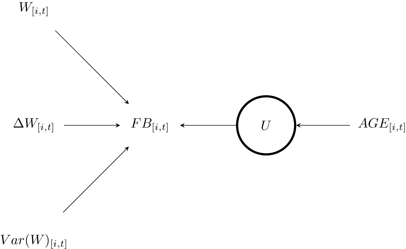


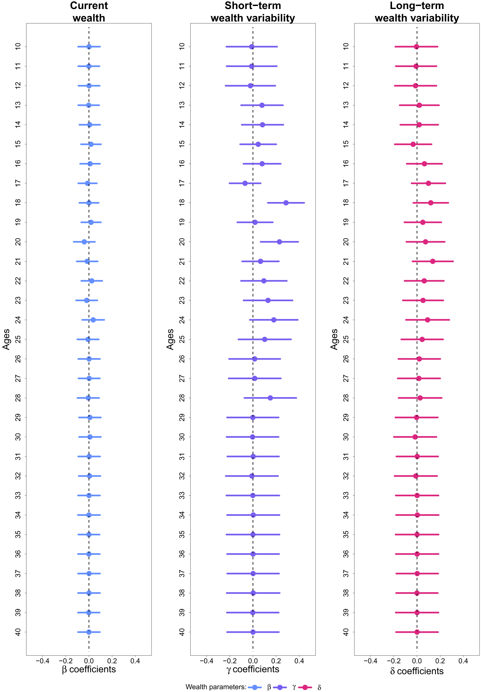


 Open access

