2.1 Notation and elementary properties

We use Dirac’s bra-ket notation. Vectors in a Hilbert space $\mathcal {H}$ will be represented as “kets” $|{\phi }\rangle $ , and the scalar product between $|{\phi }\rangle $ and $|{\psi }\rangle $ is written as $\langle {\phi }|{\psi }\rangle $ (which is antilinear in the first argument). The linear functional $|{\psi }\rangle \mapsto \langle {\phi }|{\psi }\rangle $ is then denoted as a “bra” $\langle {\phi }|$ . Rank-one linear maps will be written as $\left|{\psi }\right\rangle \!\!\left\langle {\phi }\right|$ .

Let us consider an arbitrary set $\Lambda $ , and associate to every site $x \in \Lambda $ a finite-dimensional Hilbert space $\mathcal {H}_{x} \equiv \mathbb {C}^{d}$ for a prefixed $d \in \mathbb {N}$ . As usual, for a finite subset $X \subset \Lambda $ , we define the corresponding space of states $\mathcal {H}_{X} := \otimes _{x \in X}\mathcal {H}_{x}$ and the space of bounded linear operators (observables) $\mathcal {B}_{X} := \mathcal {B}(\mathcal {H}_{X})$ endowed with the usual operator norm. We denote by the identity. We identify for $X \subset X' \subset \Lambda $ observables $\mathcal {B}_{X} \hookrightarrow \mathcal {B}_{X'}$ via the isometric embedding . Given an operator Q, the minimal region $X\subset \Lambda $ , such that $Q \in \mathcal {B}_X$ is called the support of Q. Let us observe that if $Q \in \mathcal {B}_{X}$ is a self-adjoint element, then and Q have the same eigenvalues $\lambda $ , and the corresponding eigenspaces are related via $V_{\lambda } \mapsto V_{\lambda } \otimes \mathcal {H}_{X' \setminus X}$ . In particular, . We define the spectral gap of such Q, denoted $\operatorname {gap}(Q)$ , as the difference of the two lowest (unequal) eigenvalues of Q. If Q has only one eigenvalue, we set $\operatorname {gap}(Q)=0$ .

A local Hamiltonian is defined in terms of a family of local interactions, that is, a map $\Phi $ that associates to each finite subset $Z \subset \Lambda $ a self-adjoint observable . For each finite $X \subset \Lambda $ , the corresponding Hamiltonian is the self-adjoint operator $H_{X} \in \mathcal {B}_{X}$ given by

$$\begin{align*}H_{X} = \sum_{Z \subset X}{\Phi_{Z}}\,. \end{align*}$$

Next, let us introduce some further conditions on the type of interactions we are going to deal with.

First, we are going to assume the lowest eigenvalue of $\Phi _{Z}$ is zero for each Z. This means that $\Phi _{Z} \geq 0$ , and thus $H_{X} \geq 0$ , for each finite subset $X \subset \Lambda $ . In general, from an arbitrary local interaction $\Phi _{Z}$ , we can always construct a new interaction satisfying this property by shifting each local term $\Phi _{Z}$ to , where $c_{Z}$ is the lowest eigenvalue of $\Phi _{Z}$ . As a consequence, each local Hamiltonian $H_{X}$ is shifted to , and its eigenvalues $\lambda $ are then shifted to $\lambda - (\sum _{Z \subset X} c_{Z}) $ , although the corresponding eigenspaces and the spectral gap are preserved. It should be mentioned that this shifting procedure introduces an energy constraint that can significantly impact certain physical properties of the original system. However, since our sole focus is on studying the spectral gap properties in relation to the orthogonal projectors onto the ground spaces, this argument appears reasonable for reducing the overall problem to this particular setting.

On the other hand, we are also going to assume that the local interaction $\Phi $ is frustration-free, namely, that for every finite subset $X \subset \Lambda $ , it holds that

$$\begin{align*}W_{X}:=\bigcap_{Z \subset X}{\ker(\Phi_{Z})} \neq \{0\} \,. \end{align*}$$

Let $P_{X} \in \mathcal {B}_{X}$ be the orthogonal projector onto $W_{X}$ . As a consequence of

(2.1) $$ \begin{align} \langle{\phi}|{H_X}|{\phi}\rangle = \sum_{Z\subset X} \langle{\phi}|{\Phi_Z}|{\phi}\rangle \ge 0\,, \end{align} $$

we immediately get that $\ker {(H_{X})}= W_{X}$ , and that the frustration-free condition is equivalent to each $H_{X}$ having zero as the lowest eigenvalue. In this case, $W_{X}$ is the ground space of $H_{X}$ , $P_{X}$ is the ground state projector, and the spectral gap of $H_{X}$ , in case the latter is nonzero, can be described as the largest positive constant satisfying that for every $|{\phi }\rangle \in \mathcal {H}_{X}$

(2.2) $$ \begin{align} \langle{\phi}|{P_X^{\perp}}|{\phi}\rangle \cdot \operatorname{gap}(H_{X}) \leq \langle{\phi}|{H_X}|{\phi}\rangle \,, \end{align} $$

where .

We conclude by remarking that for every $X \subset Y \subset \Lambda $ , we have $W_{Y} \subset W_{X}$ , where we are identifying $W_{X} \equiv \mathcal {H}_{Y \setminus X} \otimes W_{X}$ , and therefore $P_{Y} P_{X} = P_{Y}$ .

2.2 Spectral gap of local Hamiltonians

We will now recall a recursive strategy to obtain lower bounds to the spectral gap of frustration-free Hamiltonians described in [Reference Kastoryano and Lucia24], which we will also slightly improve over the original formulation. The main tool will be the following lemma, which is an improved version of [Reference Kastoryano and Lucia24, Lemma 14] in which the constant $(1-2c)$ has been improved to $(1-c)$ . The argument here is different and inspired by [Reference Kitaev, Shen and Vyalyi26, Lemma 14.4].

Lemma 2.1. Let $U, V, W$ be subspaces of a finite-dimensional Hilbert space $\mathcal {H}$ with corresponding orthogonal projectors $\Pi _{U}, \Pi _{V}, \Pi _{W}$ , and assume that $W \subset U \cap V$ . Then,

$$\begin{align*}\Pi_{U}^{\perp} + \Pi_{V}^{\perp} \geq (1 - c) \, \Pi_{W}^{\perp} \quad, \mbox{ where } \quad c:=\| \Pi_{U}\Pi_{V} - \Pi_{W}\|\,. \end{align*}$$

Moreover, $c \in [0,1]$ always holds, and $c \in [0,1)$ if and only if $U \cap V =W$ .

Proof. Let us start by observing that, since $W\subset U$ , it holds that $\Pi _W \Pi _U = \Pi _U \Pi _W = \Pi _W$ , and similarly for V. Thus, the constant c can be rewritten as

(2.3) $$ \begin{align} \begin{aligned} c & = \| (\Pi_{U} - \Pi_{W}) \, (\Pi_{V} - \Pi_{W}) \|\\ & = \| \Pi_{W}^{\perp} \, \Pi_{U} \, \Pi_{V} \, \Pi_{W}^{\perp}\|\\ & = \sup{\{ \, |\langle{a}| \Pi_{W}^{\perp} \, \Pi_{U} \, \Pi_{V} \, \Pi_{W}^{\perp} |{b}\rangle| \, \colon \, \| a\| \leq 1, \, \| b\| \leq 1 \rangle \}}\\ & = \sup{\{ \, | \langle{a}| \Pi_{U} \, \Pi_{V} |{b}\rangle | \, \colon \, a, b \in W^{\perp}, \, \| a\| \leq 1, \, \| b\| \leq 1 \rangle \}}\\ & = \sup{\{ \, | {\langle{a}|{b}\rangle} | \, \colon \, a \in U \cap W^{\perp}, \, b\in V \cap W^{\perp}, \, \| a\| \leq 1, \, \| b\| \leq 1 \rangle \}}. \end{aligned} \end{align} $$

From here, it immediately follows that $c \in [0,1]$ . Moreover, since $\mathcal {H}$ is finite-dimensional, the set over which the supremum is taken is compact, meaning that the supremum is always attained. Therefore, $c=1$ if and only if there exists $a\in U \cap W^{\perp }$ and $b\in V \cap W^{\perp }$ , such that $|\langle {a}| {b}\rangle | = \| a\| \| b\|$ . As the Cauchy–Schwarz inequality is only saturated by vectors which are proportional to each other, $c=1$ is equivalent to the fact that there exists an $a \in (U \cap V \cap W^{\perp }) \setminus \{ 0\}$ , or equivalently, that $W \subsetneq U \cap V$ . The first observation also implies that $\Pi _{U} = \Pi _{W} + \Pi _{W}^{\perp } \, \Pi _{U} \, \Pi _{W}^{\perp }$ and $\Pi _{V} = \Pi _{W} + \Pi _{W}^{\perp } \, \Pi _{V} \, \Pi _{W}^{\perp }$ , and therefore

$$\begin{align*}\Pi_{U}^{\perp} + \Pi_{V}^{\perp} = 2\Pi_W^{\perp} - \Pi_{W}^{\perp} \, (\Pi_{U} + \Pi_{V}) \Pi_{W}^{\perp}.\end{align*}$$

This allows us to reformulate the original inequality we aim to prove as

(2.4) $$ \begin{align} \Pi^{\perp}_{U} + \Pi_{V}^{\perp} \geq (1-c) \, \Pi_{W}^{\perp} \,\, \Leftrightarrow \,\, (1+c) \Pi_{W}^{\perp} \geq \Pi_{W}^{\perp} \, (\Pi_{U} + \Pi_{V}) \Pi_{W}^{\perp}\,. \end{align} $$

Let $|{x}\rangle $ be a norm-one eigenvector of $\Pi _{W}^{\perp } \, (\Pi _{U} + \Pi _{V}) \Pi _{W}^{\perp }$ with corresponding eigenvalue $\lambda>0$ . Note that $\Pi _{W}^{\perp } |{x}\rangle = |{x}\rangle $ necessarily, since eigenvectors with different eigenvalues are orthogonal, and W is contained in the kernel. Thus, to show that the right-hand side inequality of (2.4) holds, it is enough to check that $\lambda \leq 1+c$ necessarily. For that, let us write

$$ \begin{align*} \Pi_{U}|{x}\rangle & = \lambda_{U} \, |{x_{U}}\rangle \quad \mbox{ for some } \quad |{x_{U}}\rangle \in U \cap W^{\perp}\,, \, \langle{x_{U}}|{x_{U}}\rangle = 1\,, \, \lambda_{U} \geq 0\,,\\ \Pi_{V}|{x}\rangle & = \lambda_{V} \, |{x_{V}}\rangle \quad \mbox{ for some } \quad |{x_{V}}\rangle \in V \cap W^{\perp}\,, \, \langle{x_{V}}|{x_{V}}\rangle = 1\,, \, \lambda_{V} \geq 0\,. \end{align*} $$

On the one hand, we have

$$ \begin{align*} \lambda = \langle{x}| \Pi_{U} + \Pi_{V} |{x}\rangle & = \langle{x}| \Pi_{U} |{x}\rangle + \langle{x}| \Pi_{V} |{x}\rangle \\ & \, = \langle{x}| \Pi_{U}^{2} |{x}\rangle + \langle{x}| \Pi_{V}^{2} |{x}\rangle \\ & \, = \, \lambda_{U}^{2} + \lambda_{V}^{2}, \end{align*} $$

and, on the other hand

$$ \begin{align*} \lambda^{2} & = \langle{x}| (\Pi_{U} + \Pi_{V}) \, (\Pi_{U} + \Pi_{V}) |{x}\rangle \\ & = \lambda_{U}^{2} + \lambda_{V}^{2} + \langle{x}|\Pi_{U} \Pi_{V}|{x}\rangle + \langle{x}|\Pi_{V} \Pi_{U}|{x}\rangle \\ & = \lambda_{U}^{2} + \lambda_{V}^{2} + 2 \, \lambda_{U} \, \lambda_{V} \, \operatorname{Re}\langle{x_{U}}|{x_{V}}\rangle \,. \end{align*} $$

Combining both equalities we get, denoting $c_{x}:=|\operatorname {Re}\langle {x_{U}}|{x_{V}}\rangle |$ ,

$$ \begin{align*} (1+c_{x}) \lambda - \lambda^{2} & = c_{x} \left( \lambda_{U}^{2} + \lambda_{V}^{2} \right) - 2 \lambda_{U} \lambda_{V} \operatorname{Re}\langle{x_{U}}|{x_{V}}\rangle \\ & \geq c_{x}(\lambda_{U}^{2} + \lambda_{V}^{2} - 2 \lambda_{U} \lambda_{V}) = c_{x}(\lambda_{U} - \lambda_{V})^{2} \geq 0\,. \end{align*} $$

Since $\lambda>0$ , we conclude that

$$\begin{align*}\lambda \leq 1 + c_{x} \leq 1+c, \end{align*}$$

where the last inequality follows from (2.3). This concludes the argument.

This lemma has important implications for frustration-free local Hamiltonians, when applied to the ground state subspaces $W_X$ and their associated orthogonal projections $P_X$ . The frustration-free condition yields that, for $X, Y \subset \Lambda $ , the ground state subspaces satisfy $ W_{X \cup Y} \subset W_{X} \cap W_{Y}$ . As a consequence of Lemma 2.1,

$$\begin{align*}\| P_{X \cup Y} - P_{X} P_{Y}\| = \| (P_{X \cup Y} - P_{X}) (P_{X \cup Y} - P_{Y})\| \in [0, 1]\,. \end{align*}$$

Moreover, $W_{X \cup Y} = W_{X} \cap W_{Y}\,$ if and only if $\| P_{X \cup Y} - P_{X} P_{Y}\| \in [0, 1)$ . This happens whenever $\Lambda $ is a metric space, $\Phi $ has finite range $r>0$ , namely, that $\Phi _{X}=0$ if the diameter of X is larger than r, and the distance $d(X \setminus Y, Y \setminus X)$ is greater than r, since in this case, every subset $Z \subset X \cup Y$ with $\Phi _{Z} \neq 0$ is either contained in X or Y, so that

$$\begin{align*}W_{X \cup Y} = \bigcap_{Z \subset X \cup Y} \ker{\Phi_{Z}} = \bigcap_{Z \subset X} \ker{\Phi_{X}} \cap \bigcap_{Z \subset Y} \ker{\Phi_{Z}} = W_{X} \cap W_{Y} \,. \end{align*}$$

Definition 2.2 (Spectral gap).

For each finite subset $Y \subset \Lambda $ , let us denote by $\operatorname {gap}(H_{Y})$ , or simply $\operatorname {gap}(Y)$ , the spectral gap of $H_{Y}$ , namely, the difference between the two lowest unequal eigenvalues of $H_{Y}$ . If it has only one eigenvalue, then we define $\operatorname {gap}(Y) = 0$ . Given a family $\mathcal {F}$ of finite subsets of $\Lambda $ , we say that the system of Hamiltonians $(H_{Y})_{Y \in \mathcal {F}}$ is gapped whenever

$$\begin{align*}\operatorname{gap}(\mathcal{F}):=\inf{\{ \operatorname{gap}(Y) \colon Y \in \mathcal{F} \}}> 0\,. \end{align*}$$

Otherwise, it is said to be gapless.

The following result allows to relate the gap of two families. It adapts a result from [Reference Kastoryano and Lucia24, Section 4.2].

Theorem 2.3. Let $\mathcal {F}$ and $\mathcal {F}'$ be two families of finite subsets of $\Lambda $ . Suppose that there are $s \in \mathbb {N}$ and $\delta \in [0,1]$ satisfying the following property: for each $Y \in \mathcal {F}' \setminus \mathcal {F}$ , there exist $(A_{i}, B_{i})_{i=1}^{s}$ pairs of elements in $\mathcal {F}$ , such that:

1. (i) $Y = A_{i} \cup B_{i}$ for each $i=1, \ldots , s$ ,

2. (ii) $(A_{i} \cap B_{i}) \cap (A_{j} \cap B_{j}) = \emptyset $ whenever $i \neq j$ ,

3. (iii) $\|P_{A_{i}}P_{B_{i}} - P_{Y}\| \leq \delta $ for every $i=1, \ldots , s$ .

Then,

$$\begin{align*}\operatorname{gap}(\mathcal{F}') \, \geq \, \frac{1-\delta}{1+ \frac{1}{s}} \, \operatorname{gap}(\mathcal{F}) \, \underset{(\text{if }\delta < 1)}{\geq} \, \exp\left[ -\frac{\delta}{1- \delta} - \frac{1}{s}\right] \, \operatorname{gap}(\mathcal{F}) \,. \end{align*}$$

Proof of Theorem 2.3.

Let $Y \in \mathcal {F}' \setminus \mathcal {F}$ , and let $(A_{i}, B_{i})_{i=1}^{s}$ be the family of pairs satisfying $(i)$ – $(iii)$ provided by the hypothesis. To prove the first inequality, we can assume that $\delta < 1$ and $\operatorname {gap}(\mathcal {F})>0$ , since otherwise, the inequality is obvious. Applying Lemma 2.1, and using (2.2), we can estimate

$$ \begin{align*} \langle{x}| P_{Y}^{\perp} |{x}\rangle \, = \, \frac{1}{s} \sum_{i=1}^{s}{\langle{x}| P_{Y}^{\perp} |{x}\rangle } \,\, & \leq \,\, \frac{1}{s} \sum_{i=1}^{s} \frac{1}{1-\delta} \left(\langle{x}| P_{A_{i}}^{\perp} |{x}\rangle + \langle{x}| P_{B_{i}}^{\perp} |{x}\rangle \right) \\ & \leq \,\, \frac{1}{1-\delta} \, \frac{1}{s} \sum_{i=1}^{s} \frac{1}{\operatorname{gap}(\mathcal{F})} \left(\langle{x}| H_{A_{i}} |{x}\rangle + \langle{x}| H_{B_{i}} |{x}\rangle \right)\\ & \leq \,\, \frac{1}{1-\delta} \, \frac{1}{\operatorname{gap}(\mathcal{F})} \, \frac{1}{s} \sum_{i=1}^{s} \langle{x}| H_{Y} + H_{A_{i} \cap B_{i}} |{x}\rangle \\ & \leq \,\, \frac{1}{1- \delta} \, \frac{1}{\operatorname{gap}(\mathcal{F})} \, \, \langle{x}| H_{Y} + \frac{1}{s} \sum_{i=1}^{s} H_{A_{i} \cap B_{i}} |{x}\rangle \\ & \leq \,\, \frac{1}{1- \delta} \, \frac{1}{\operatorname{gap}(\mathcal{F})} \, \, \left( 1+ \frac{1}{s} \right) \, \langle{x}| H_{Y} |{x}\rangle \,. \end{align*} $$

Notice that in the third line, we have used that $H_{A_{i}} + H_{B_{i}} \leq H_{Y} + H_{A_{i} \cap B_{i}}$ , which holds since all the local interactions are positive semidefinite. Therefore, again by (2.2), it holds that

$$\begin{align*}\operatorname{gap}(Y) \geq \frac{1- \delta}{1+\frac{1}{s}} \, \operatorname{gap}(\mathcal{F})\quad \text{whenever} \quad Y \in \mathcal{F}' \setminus \mathcal{F}\,. \end{align*}$$

On the other hand, if $Y \in \mathcal {F}' \cap \mathcal {F}$ , then $\operatorname {gap}(Y) \geq \operatorname {gap}(\mathcal {F}) $ by definition. Hence, we conclude the that the first inequality holds. To obtain the second inequality, we simply use twice that $(1+x)^{-1} \geq e^{-x}$ for every $x \geq 0$ .

In the next section, we will apply Theorem 2.3 in order to bound the spectral gap of a quantum spin Hamiltonian on an arbitrarily large torus (with periodic boundary conditions) in terms of the spectral gap of the same model on a finite family of rectangles with open boundary conditions. This is reminiscent to the bounds on the spectral gap based on the local gap thresholds [Reference Anshu3, Reference Gosset and Mozgunov18, Reference Lemm and Mozgunov20, Reference Lemm21, Reference Knabe27]. The reason for which we are following a different approach is that the constants appearing in the spectral gap thresholds are highly dependent on the specific shape and range of the interactions of the Hamiltonian, and in our case, we will have to consider $\beta $ -dependent interaction length. Therefore, it will be unfeasible to verify the local gap threshold conditions for our models. The connection between the control of quantities of the type ${\lVert }{P_{X\cup Y} - P_X P_Y}{\rVert }$ and spectral gap estimates originated in the seminal work on finitely correlated states [Reference Fannes, Nachtergaele and Werner16], later extended to more general spin models [Reference Nachtergaele32]. The main difference between that approach and the one of [Reference Kastoryano and Lucia24], which we are following here, is due to the way in which we are growing the lattice: while the methods of [Reference Fannes, Nachtergaele and Werner16, Reference Nachtergaele32] consider a single increasing sequence of regions, Theorem 2.3 permits more rich families of subsets, thus allowing us to keep the shape of their intersections more well-behaved (i.e., they will always be rectangles or cylinders).

2.3 Periodic boundary conditions on a torus

To describe the periodic boundary conditions case, we have to introduce further notation. For each natural N, let us denote by $\mathbb {S}_{N}$ the quotient $\mathbb {R}/\sim $ , where we relate $x \sim x+N$ for every $x \in \mathbb {R}$ . Note that we can identify $\mathbb {S}_{N} \equiv [0, N)$ .

We will take as $\Lambda _{N}$ , the set where the spins of the system are located, the set of midpoints of the edges $\mathcal {E}_{N}$ of the square lattice on the torus $\mathbb {S}_{N} \times \mathbb {S}_{N}$ (as this is the setting in which the quantum double models are defined). We will identify each point of $\Lambda _{N}$ with the corresponding edge from $\mathcal {E}_{N}$ , so that we will indistinctly use $\Lambda _{N}$ or $\mathcal {E}_{N}$ (see Figure 1).

Figure 1

The square lattice on the torus (left), and the quantum spin system with spins on the midpoints of the edges (right). The marks on the borders of both squares represent the pairwise identification of edges, a standard depiction of the torus in topology. A similar notation will be used for the cylinder, where only one pair of edges is identified.

Let us recall the notion of a (closed) interval in $\mathbb {S}_{N}$ . Given $x,y \in \mathbb {S}_{N}$ , we denote by $d_{+}(x,y)$ the unique $0 \leq c < N$ , such that $x+c \sim y$ . Then, we define the interval $[a,b]$ as the set $\{ x \in \mathbb {S}_{N} \colon d_{+}(a, x) \leq d_{+}(a,b) \}$ . We are only going to consider intervals with integer endpoints, that is, $a,b \in \mathbb {Z}_{N}$ . A proper rectangle $\mathcal {R}$ in $\mathbb {R}^{2}$ or $\mathbb {S}_{N} \times \mathbb {S}_{N}$ is a Cartesian product of intervals $\mathcal {R}=[a_{1}, b_{1}] \times [a_{2}, b_{2}]$ (with integer endpoints). Its number of plaquettes per row is then $d_{+}(a_{1},b_1)$ and per column is $d_{+}(a_{2},b_2)$ . Shortly, we say that $\mathcal {R}$ has dimensions $d_{+}(a_{1},b_1)$ and $d_{+}(a_{2},b_2)$ . A cylinder is a Cartesian product of the form $\mathbb {S}_{N} \times [a,b]$ or $[a,b] \times \mathbb {S}_{N}$ . We will refer simply as rectangles to proper rectangles, cylinders, and the whole torus $\mathbb {S}_{N} \times \mathbb {S}_{N}$ . In an abuse of notation, we will identify $\mathcal {R}$ with $\mathcal {R} \cap \Lambda $ and often write $\mathcal {R} \subset \Lambda $ and $\mathcal {H}_{\mathcal {R}}$ to denote the associated Hilbert space (see Figure 2).

Figure 2

Examples of rectangles as a subset of the square lattice $\Lambda _{N} \equiv \mathcal {E}_{N}$ . Above, two examples of proper rectangles, whereas below, two examples of cylinders. In each case, we present two pictures: on the right, we highlight the spins belonging to the region, while on the left, we highlight the edges. We will use this latter representation in the forthcoming pictures.

We are going to define, for every $N,r \in \mathbb {N}$ with $N \geq r \geq 2$ , the following sets of rectangular regions in $\mathcal {E}_{N}$ :

• $\triangleright $ $\mathcal {F}_{N}$ is the set of all rectangular regions having at least two plaquettes per row and per column.

• $\triangleright $ $\mathcal {F}_{N}^{torus}$ is the family consisting of only one element, the whole torus.

• $\triangleright $ $\mathcal {F}_{N}^{cylin}$ is the family of all cylinders having at least two plaquettes per row and per column.

• $\triangleright $ $\mathcal {F}_{N, r}^{rect}$ is the family of all proper rectangles having at least two and at most r plaquettes per row and per column.

Martingale condition on local projectors

For each $X \in \mathcal {F}_{N}$ , let $\Pi _{X}$ be an orthogonal projector onto a subspace of $\mathcal {H}_{X}$ , such that $(\Pi _{X})_{X}$ satisfies the frustration-free condition: $\Pi _{X} \Pi _{Y}=\Pi _{Y}\Pi _{X} =\Pi _{Y}$ for every pair of rectangular regions $X \subset Y$ . Notice that the family of projectors $(P_{X})_{X}$ associated to a frustration-free Hamiltonian, as it was defined in Section 2.1, satisfies this condition.

Estimating the gap from below

Let us fix a local interaction $\Phi $ on the torus $\mathcal {E}_{N}$ defining a frustration-free Hamiltonian. For each rectangular region $X \subset \mathcal {E}_{N}$ , let us denote by $P_{X}$ the orthogonal projector onto the ground space of $H_{X}$ . Let us, moreover, assume that the family of projectors $(P_{X})_{X}$ satisfies the martingale condition for a decay function $\delta (\ell )$ as in Definition 2.4.

Theorem 2.5. If $\delta (\lfloor N/2-1 \rfloor )<1/2$ , then

$$\begin{align*}\operatorname{gap}(\mathcal{F}_{N}^{torus}) \, \geq \, \frac{1}{4} \operatorname{gap}(\mathcal{F}_{N}^{cylin}) \, \geq \, \frac{1}{16} \operatorname{gap}(\mathcal{F}_{N,N}^{rect})\,.\end{align*}$$

Proof. Let us first compare $\operatorname {gap}(\mathcal {F}_{N}^{torus})$ and $\operatorname {gap}(\mathcal {F}_{N}^{cylin})$ . We consider a decomposition of the torus $\Lambda _{N}$ into four regions $A,B,C,B'$ as in (2.8), so that $\mathcal {C}_{1}:=B'AB$ and $\mathcal {C}_{2}:=BCB'$ are cylinders having dimensions $N-1$ and N belonging to $\mathcal {F}_{N}^{cylin}$ and whose intersection consists of two cylinders B and $B'$ , each having N plaquettes per column and at least $\lfloor N/2-1\rfloor $ plaquettes per row.

(2.8)

Applying the martingale condition from Definition 2.4 (iii), we deduce that

(2.9) $$ \begin{align} \| P_{\mathcal{C}_{1}} P_{\mathcal{C}_{2}} - P_{\Lambda_{N}} \| \, \leq \, \delta(\lfloor N/2-1 \rfloor) < \frac{1}{2}\,, \end{align} $$

and so, by Theorem 2.3 with $s=1$ and $\delta =1/2$ , we can estimate

$$\begin{align*}\operatorname{gap}(\mathcal{F}_{N}^{torus}) \, \geq \, \frac{1}{4} \, \operatorname{gap}(\mathcal{F}_{N}^{cylin}) \,. \end{align*}$$

Next, we compare $\mathcal {F}_{N}^{cylin}$ and $\mathcal {F}_{N,N}^{rect}$ . Given a cylinder $\mathcal {C} \in \mathcal {F}_{N}^{cylin}$ , we can split it along the wrapping direction into four regions $A,B,C,B'$ as in (2.10), so that $\mathcal {R}_{1}:=B'AB$ and $\mathcal {R}_{2}:=BCB'$ are proper rectangles having N plaquettes along the splitting direction, belonging to $\mathcal {F}_{N}^{rect}$ , and whose intersection consists of two proper rectangles B and $B'$ having at least $\lfloor N/2-1 \rfloor $ plaquettes along the splitting direction.

(2.10)

Thus, applying the martingale condition from Definition 2.4(ii), we deduce that

$$\begin{align*}\| P_{\mathcal{R}_{1}} P_{\mathcal{R}_{2}} - P_{\mathcal{C}} \| \, \leq \, \delta(\lfloor N/2-1 \rfloor) < \frac{1}{2}\,, \end{align*}$$

and so, by Theorem 2.3 with $s=1$ and $\delta =1/2$ , we can estimate

(2.11) $$ \begin{align} \operatorname{gap}(\mathcal{F}_{N}^{cylin}) \, \geq \, \frac{1}{4} \, \operatorname{gap}(\mathcal{F}_{N,N}^{rect})\,. \end{align} $$

Combining (2.9) and (2.11), we conclude the result.

Theorem 2.6. For fixed integers $N \geq r \geq 16$ , let us denote $\delta _{k}:= \delta (\lfloor \tfrac {r}{4}(\sqrt {9/8}\,)^{k}\rfloor \,)$ and $s_k:=\lfloor (\sqrt {4/3}\,)^{k} \rfloor $ for each integer $k \geq 0$ . Then, we can estimate from below

$$\begin{align*}\operatorname{gap}(\mathcal{F}_{N,N}^{rect}) \, \geq \, \left(\, \prod_{k=0}^{\infty} \frac{1-\delta_{k}}{1+\frac{1}{s_{k}}}\right) \, \operatorname{gap}(\mathcal{F}^{rect}_{N,r})\,. \end{align*}$$

Notice that the infinite product that appears in the previous expression is convergent to a positive value whenever the decay function $\delta (\ell )$ decays polynomially fast, namely, $\delta (\ell ) = O(\ell ^{-\alpha })$ for some $\alpha>0$ .

Proof. The idea of the proof is inspired by [Reference Cesi9]. Fix $N,r$ as above, for each $k \geq 0$ , let $\mathcal {G}_{k}$ be the family of all proper rectangles in $\mathcal {F}_{N,N}^{rect}$ of dimensions a and b satisfying

$$\begin{align*}a,b \geq 2 \quad \mbox{ and } \quad a \cdot b \leq r (3/2)^{k}\,.\end{align*}$$

Observe that $\mathcal {G}_{k} \subset \mathcal {G}_{k+1}$ for every $k \geq 0$ and that $\mathcal {G}_{k} = \mathcal {F}_{N,N}^{rect}$ for k large enough. Next, let $Y \in \mathcal {G}_{k+1} \setminus \mathcal {G}_{k}$ of dimensions a and b. Then

$$\begin{align*}r (3/2)^{k} < a \cdot b \leq r (3/2)^{k+1}\,. \end{align*}$$

We can assume without loss of generality that $a \leq b$ , so using the previous inequalities, we can estimate from below (recall that $r \geq 16$ )

(2.12) $$ \begin{align} 4 \leq \sqrt{r} (\sqrt{3/2}\,)^{k} \leq b\,. \end{align} $$

Let us define

$$\begin{align*}s_{k}:= \lfloor (\sqrt{4/3}\,)^{k} \rfloor \quad \mbox{and} \quad \ell_{k} := \left\lfloor b/(4 s_{k}) \right\rfloor \,. \end{align*}$$

Observe that by (2.12)

(2.13) $$ \begin{align} \ell_{k} \geq \left\lfloor\frac{b}{4s_{k}}\right\rfloor \geq \left\lfloor \frac{\sqrt{r}}{4} (\sqrt{3/2}\,)^{k} (\sqrt{3/4}\,)^{k} \right\rfloor = \left\lfloor\frac{\sqrt{r}}{4} (\sqrt{9/8}\,)^{k}\right\rfloor \geq 1\,, \end{align} $$

and for every $j = 0, \ldots , s_{k}-1$

(2.14) $$ \begin{align} (2j+1) \ell_{k} \leq 2 s_{k} \ell_{k} -\ell_{k} \leq \frac{b}{4}-1\,. \end{align} $$

Next, let us identify our rectangle Y with $[0,b] \times [0,a]$ , and consider the subrectangles (see Figure 3)

$$ \begin{align*} A_{j} := \left[0, \lceil b/3 \rceil + (2j+1) \ell_k \, \right] \times [0,a] \quad ,\quad B_{j} := \left[\lceil b/3 \rceil + 2j \ell_k, b \, \right] \times [0,a] \,. \end{align*} $$

Note that, applying (2.14), we deduce that $A_{j}$ is contained in a rectangle of dimensions a and $\lceil b/3\rceil +b/4-1 \leq 2b/3$ . Similarly, $B_{j}$ is contained in a rectangle of dimensions a and $b-\lceil b/3 \rceil \leq 2b/3$ . Since $a \geq 2$ , $2b/3 \geq 2$ , and $a \cdot (2b/3) \leq r(3/2)^{k}$ , we conclude that $A_{j}, B_{j} \in \mathcal {G}_{k}$ by definition. Moreover, the intersections

$$\begin{align*}A_{j} \cap B_{j} = \left[ \, \lceil b/3 \rceil + 2j \ell_k, \lceil b/3 \rceil + (2j+1) \ell_k \, \right] \times [0,a] \, \end{align*}$$

are disjoint, that is $A_{j} \cap B_{j} \cap A_{j'} \cap B_{j'} = \emptyset $ whenever $j \neq j'$ , and have $\ell _{k}$ plaquettes per row and a plaquettes per column. Using the martingale condition from Definition 2.4(i) and (2.13)

$$\begin{align*}\| P_{A_{j}} P_{B_{j}} - P_{Y} \| \leq \delta(\ell_{k}) \leq \delta(\lfloor\tfrac{\sqrt{r}}{4}(\sqrt{9/8})^{k}\rfloor)\,.\end{align*}$$

Figure 3

Split of the rectangle Y in the proof of Theorem 2.6. The thick subrectangles correspond to the intersections $A_{i} \cap B_{i}$ , being disjoint and having width equal to $\ell _{k}$ .

Applying now Theorem 2.3, we deduce that

$$\begin{align*}\operatorname{gap}(\mathcal{G}_{k+1}) \geq \frac{1-\delta_{k}}{1+\frac{1}{s_{k}}} \operatorname{gap}(\mathcal{G}_{k}) \geq \ldots \geq \, \left(\prod_{j=0}^{k} \frac{1-\delta_{j}}{1+\frac{1}{s_{j}}}\right) \,\, \operatorname{gap}(\mathcal{G}_{0})\,. \end{align*}$$

Finally, noticing that $\mathcal {G}_{0} \subset \mathcal {F}_{r,N}^{rect}$ , we conclude the result.

3.1 Tensor notation

Let us denote $[d]:=\{ 0,1,\ldots , d-1\}$ for each $d \in \mathbb {N}$ . Recall that a tensor with n indices is simply an element $T \in \mathbb {C}^{[d_{1}] \times \ldots \times [d_{n}]} $ , where each $d_{j} \in \mathbb {N}$ is called the dimension of the j-th index. We will employ the usual notation

$$\begin{align*}T_{\alpha} = T_{\alpha_{1} \ldots \alpha_{n}} \quad , \quad \alpha = (\alpha_{1}, \ldots, \alpha_{n}) \in [d_{1}] \times \ldots \times [d_{n}]\,. \end{align*}$$

By definition, a tensor with zero indices will be a scalar $T \in \mathbb {C}$ . We can represent tensors in the form of a ball with a leg for each index:

Let us describe the basic operations that we will perform with tensors. Given a tensor with (at least) two indices, say $\alpha _{1}$ and $\alpha _{2}$ with dimensions $d_{1}$ and $d_{2}$ , respectively, we can combine them into one index $\gamma $ of dimension $d_{1}\cdot d_{2}$ , so that the resulting tensor has one index less. This process can be iterated to combine several indices into one index. Graphically, we have the following example:

Given two tensors $T=(T_{\alpha })$ and $S=(S_{\beta })$ with m and n indices, respectively, we define its tensor product as the unique tensor with $n+m$ indices given by $T \otimes S :=(T_{\alpha } \cdot S_{\beta })$ . For instance:

If a tensor $(T_{\alpha })$ has two indices with the same dimension, say $\alpha _{1}$ and $\alpha _{2}$ , then we can contract them, resulting in a tensor with $n-2$ indices $S_{\alpha _{3} \ldots \alpha _{n}} = \sum _{j} T_{jj\alpha _{3}\ldots \alpha _{n}}$ . Combining this operation with the tensor product of tensors, we define the contraction of tensors: given two tensors $(T_{\alpha })$ and $(S_{\beta })$ having both an index with the same dimension, say $\alpha _{1}$ and $\beta _{1}$ , we can contract these indices to generate a new tensor $(\sum _{j}T_{j\alpha _{2}\ldots \alpha _{n}} \cdot S_{j\beta _{2}\ldots \beta _{m}})$ . Graphically, we have the following example:

If two tensors have the same indices with the same dimensions $(T_{\alpha })_{\alpha }$ and $(S_{\alpha })_{\alpha }$ , we can define their tensor sum $T+S:=(T_{\alpha }+S_{\alpha })_{\alpha }$ . Given a tensor $(T_{\alpha })_{\alpha }$ and a scalar $\lambda \in \mathbb {C}$ , we define $\lambda T := (\lambda T_{\alpha })_{\alpha }$ .

If we identify each index j with a Hilbert space $\mathbb {C}^{d_{j}}$ , we can interpret a tensor T as the coefficients of a ket $|{\psi }\rangle $ in the computational basis

$$\begin{align*}|{\psi}\rangle \in \otimes_{j=1}^{n} \mathbb{C}^{d_{1}} \quad , \quad |{\psi}\rangle = \sum_{\alpha_{1}, \ldots, \alpha_{n}} T_{\alpha_{1} \ldots \alpha_{n}} |{\alpha_{1} \ldots \alpha_{n}}\rangle\,. \end{align*}$$

More generally, if we split the set of indices into two subsets A and B called input and output indices, respectively, we can then associate to T the operator

$$\begin{align*}T: \otimes_{j \in A} \mathbb{C}^{d_{j}} \longrightarrow \otimes_{j \in B}\mathbb{C}^{d_{j}} \quad , \quad \sum_{\alpha} T_{\alpha} |{\alpha_{B}}\rangle \langle{\alpha_{A}}| \,, \end{align*}$$

where $|{\alpha _{J}}\rangle = \otimes _{j \in J} |{\alpha _{j}}\rangle $ for any subset of indices J. Following the graphical description, we will represent input (respectively, output) indices with arrows that will point at (away from) the ball. For instance, in the case of a tensor with five legs $(T_{\alpha _{1} \ldots \alpha _{5}})$ , we can consider

We will take advantage of these multiple interpretations to find easy descriptions of tensors. For instance, the tensor T with four indices of dimension two given by $T_{0 0 0 0} = T_{1 1 1 1} =1, T_{0 1 1 0} = T_{1 0 0 1}=-1$ and $T_{\alpha _{1} \alpha _{2} \alpha _{3} \alpha _{4}}=0$ , otherwise, can be represented as

Simple descriptions of a tensor can also be obtained by taking linear combinations of tensors having the same number of indices and the same dimensions. For instance, the tensor T with four indices of dimension two given by $T_{0 0 0 0} = T_{1 1 1 1} =1$ and $T_{\alpha _{1} \alpha _{2} \alpha _{3} \alpha _{4}}=0$ , otherwise, can be represented as

Finally, we can also represent the previous tensor as the contraction of two tensors, namely

(3.1)

3.2 PEPS

Let us recall the notation and main concepts for PEPS [Reference Cirac, Pérez-García, Schuch and Verstraete10, Reference Cirac, Garre-Rubio and Pérez-García11]. Let us consider a finite graph consisting of a finite set of vertices $\Lambda $ and a set of edges E. At each vertex $x \in \Lambda $ , consider a tensor in the form of an operator

Here, $\mathbb {C}^{d}$ is the physical space associated with x and each $\mathbb {C}^{D}$ is the virtual space corresponding to an edge $e \in \partial x$ , the set of edges incident to x (in the figure, we have shown the case ${|}{\partial x}{|} =4$ ).

For a finite region $X \subset \Lambda $ , we can assign the tensors $V_{x}$ to each site $x \in X$ and perform contractions between pairs of sites $x, y \in X$ that share an edge e. Specifically, we contract the two virtual indices from $V_{x}$ and $V_{y}$ that are associated with the same edge e. The contraction of the PEPS tensors gives a linear map from the virtual edges $\partial X$ connecting X with its complement to the bulk physical Hilbert space, which we denote as

$$\begin{align*}V_X : \mathcal{H}_{\partial X} \longrightarrow \mathcal{H}_{X}\,, \end{align*}$$

where we can identify $\mathcal {H}_{\partial X} \equiv (\mathbb {C}^{D})^{\otimes \partial X}$ and $\mathcal {H}_{X} \equiv (\mathbb {C}^{d})^{\otimes X}$ . The image of $V_X$ is the space of physical states which can be represented by the PEPS with an appropriate choice of boundary condition.

The boundary state on region X is defined as

(3.2)

If $\rho _{\partial X}$ has full rank, we say that the PEPS is injective on region X. If the PEPS is injective on every sufficiently large region X, we will simply say that it is injective. We will denote by $J_{\partial X}$ the orthogonal projector onto the support of $\rho _{\partial X}$ .

If we replace the physical space $\mathbb {C}^d$ with a space of operators $\mathcal {B}(\mathbb {C}^d)$ , then we talk of Projected Entangled-Pair Operators (PEPOs) instead. If we fix a basis of matrix units $\{ \left|{i}\right\rangle \!\left\langle {j}\right| \}_{i,j=1}^{d}$ for $\mathcal {B}(\mathbb {C}^d)$ (although we will find it convenient to sometimes work with different bases), then the single-site tensor $V_x$ takes the form:

In the formula, we have separated the physical indices, given by the matrix units $\left|{i}\right\rangle \!\left\langle {j}\right|$ , from the virtual indices. In the figures, we add arrows on the physical indices to indicate which spaces correspond to the “ket” and “bra” part of $\left|{i}\right\rangle \!\left\langle {j}\right|$ , see, for example, (3.1). A particularly simple case of a PEPO is when the lattice is simply a 1D ring of n sites, in which case, it is also called an MPO. These will be the building blocks for our PEPO constructions. An MPO is any operator that can be written as

$$\begin{align*}\sum_{i_1,\dots,i_n=1}^{d^2} \operatorname{Tr} \left[ M^{(1)}_{i_1} \cdots M^{(n)}_{i_n} \right] B^{(1)}_{i_1} \otimes \cdots \otimes B^{(n)}_{i_n}, \end{align*}$$

where, for each site $k=1,\dots , n$ , we have fixed a basis $\{ B^{(k)}_i \}_{i=1}^{d^2}$ of $\mathcal {B}(\mathbb {C}^d)$ and a set of $d^2$ matrices $\{ M^{(k)}_i \}_{i=1}^{d^2}$ of dimension $D\times D$ . To pass from an MPO to a PEPO representation, it is sufficient to check that the single site tensor

$$\begin{align*}V_{k} = \sum_{i=1}^{d^2} B^{(k)}_i \otimes \sum_{\alpha, \beta = 1}^D (M^{(k)}_{i})_{\alpha,\beta} \langle{\alpha, \beta}|, \end{align*}$$

where $(M^{(k)}_{i})_{\alpha ,\beta }$ denotes the matrix units of $M^{(k)}_{i}$ , represents the same operator. It will be convenient to have a “hybrid” representation of a PEPO, in which the virtual level is still represented as a matrix, that is by writing

$$\begin{align*}V_{k} = \sum_{i=1}^{d^2} B^{(k)}_i \otimes M^{(k)}_{i}, \end{align*}$$

as this allows a more direct calculation of the tensor contractions.

Note that we can always represent a PEPO as a PEPS with physical space $\mathbb {C}^d \otimes \mathbb {C}^d$ , by choosing an orthonormal basis of $\mathcal {B}(\mathbb {C}^d)$ in order to identify that space with $\mathbb {C}^d \otimes \mathbb {C}^d$ . If we choose the basis given by matrix units $\{ \left|{i}\right\rangle \!\left\langle {j}\right|\}_{i,j=1}^d$ , then this identification can be done as follows. Let $|{\Psi }\rangle = (\sum _{i=1}^d |{i,i}\rangle )^{\otimes |{\mathcal {R}} |}$ be a maximally entangled state on $\mathcal {H}_{\mathcal {R}} \otimes \mathcal {H}_{\mathcal {R}}$ . Each operator $Q \in \mathcal {B}(\mathcal {H}_{\mathcal {R}})$ can be represented in “vector form” by

The map $Q \mapsto |{Q}\rangle $ is an isometry between $\mathcal {B}(\mathcal {H}_{\mathcal {R}})$ with the Hilbert-Schmidt scalar product and $\mathcal {H}_{\mathcal {R}} \otimes \mathcal {H}_{\mathcal {R}}$ . We should mention that, if $\rho \in \mathcal {B}(\mathcal {H}_{\mathcal {R}})$ is a positive PEPO (in the sense that it is a positive operator in the range of the map $V_{\mathcal {R}}$ for some region $\mathcal {R}$ ), it is not always true that it admits a local purification, in the sense that there exists a PEPS on a doubled physical space $\mathcal {H}_{\mathcal {R}} \otimes \mathcal {H}_{\mathcal {R}}$ , such that we recover $\rho $ when we trace out one of the copies of $\mathcal {H}_{\mathcal {R}}$ . On the other hand, in the case when $\rho ^{1/2}$ is a PEPO, then $|{\rho ^{1/2}}\rangle $ is a PEPS and a purification of $\rho $ . Therefore, when studying the case in which $\rho _{\beta }$ is the Gibbs state of a local, commuting Hamiltonian at inverse temperature $\beta $ , we will write a PEPO representation for $\rho _{\beta }^{1/2}$ (which is proportional to $\rho _{\beta /2}$ up to normalization), and from it, we will obtain the PEPS representation for the thermofield double state $|{\rho _{\beta }^{1/2}}\rangle $ .

Let us briefly discuss some characteristics that the PEPS description of the thermofield double state will have. It will be convenient for us to consider a more general definition of PEPS in which the underlying graph $(\Lambda , E)$ can be a multigraph. This means that there might be multiple edges joining the same pair of different vertices of $\Lambda $ . Of course, we might combine virtual indices joining the same pair of sites into only one virtual index, adhering to the original definition of PEPS on graphs, as we represent in the next picture:

However, as we will see in Section 4, when finding the PEPS description of the thermofield double state, it is more natural and useful using the representation with the multigraph, especially when applying results, such as Theorem 3.5, that require a suitable arrangement of the set of all virtual indices of $V_{X}$ for a region X into several subsets. In the setting of the quantum double model, recall that $\Lambda _{N}$ is the set of edges $\mathcal {E}_{N}$ of the squared lattice on the torus. It is important not to confuse this set of edges with the set of edges $E_{N}$ joining the sites in $\Lambda _{N}$ and define the PEPS. In this case, every site $x \in \Lambda _{N}$ will be connected to the other four sites via two edges of $E_{N}$ as in the next picture:

If G is the finite group from which the quantum double model will be constructed, then the individual tensor $V_{x}$ will have as physical space $\mathbb {C}^{{|{G}|}}$ , and each virtual space will correspond to $\mathbb {C}^{|G|}$ :

3.3 Parent Hamiltonian

A parent Hamiltonian of a PEPS is a local, frustration-free Hamiltonian whose local ground state spaces $W_{\mathcal {R}}$ coincide with the range of $V_{\mathcal {R}}$ for all sufficiently large regions $\mathcal {R}$ .

There are well-known conditions that can be imposed on the local PEPS tensors $V_x$ that ensure that a parent Hamiltonian exists (in which case, it will not be unique), one of which is injectivity [Reference Pérez-García, Verstraete, Cirac and Wolf36], and which can be generalized to G-injectivity and MPO-injectivity. Since the PEPS we will consider will not satisfy any of them, we omit further details in this direction, and we will prove directly the existence of a parent Hamiltonian in Section 4.5.

For a given PEPS, there is a canonical construction of a local and frustration-free Hamiltonian whose local ground spaces contain the range of $V_{\mathcal {R}}$ . For every finite subset X of $\Lambda $ , let $P_{X}:\mathcal {H}_{X} \longrightarrow \mathcal {H}_{X}$ be the orthogonal projector onto $\operatorname {Im} (V_{X})$ . Note that if $X \subset Y$ , then $\operatorname {Im} (V_{Y}) \subset Im (V_{X}) \otimes \mathcal {H}_{Y \setminus X}$ . Thus, the projectors satisfy the frustration-free condition $P_{X}P_{Y}=P_{Y}P_{X}=P_{Y}$ , or also, $P_{X}^{\perp } \geq P_{Y}^{\perp }$ .

Next, let us fix a certain family $\mathcal {X}$ of subsets of $\Lambda $ having small range, for example, rectangular regions in $\Lambda = \mathbb {Z}^{2}$ of dimensions $r \times r$ for a fixed value r. Then, consider the local interaction defined by the operators . Note that for each finite region R, the local Hamiltonian

$$\begin{align*}H_{\mathcal{R}} = \sum_{X \in \mathcal{X} \, , \, X \subset \mathcal{R}} P_{X}^{\perp}\end{align*}$$

satisfies $\operatorname {Im} (V_{R}) \subset \ker {H_{R}}$ , so that the PEPS is in the ground space of this Hamiltonian. For this to be a parent Hamiltonian, we need a condition ensuring that this is indeed an equality for large enough regions. We will now show that such condition can be obtained starting from the martingale condition (see Definition 2.4). As the result is not specific to PEPS, we will state it here in its full generality.

Let us consider the setting of a quantum spin system over a finite set $\Lambda $ that we presented at the beginning of Section 2.3. Let us assume that for each finite subset X, we have an orthogonal projector $P_{X}$ onto a subspace of $\mathcal {H}_{X}$ satisfying the frustration-free condition $P_{X}P_{Y} = P_{Y}P_{X}=P_{Y}$ for every pair of subsets $X \subset Y$ . In the case of a PEPS, these projections will be the ones onto $\operatorname {Im} (V_{X})$ .

Lemma 3.1. Under the setting just described, fix a family $\mathcal {X}$ of finite subsets of $\Lambda $ , and consider the local interactions , $X \in \mathcal {X}$ defining for each finite $\mathcal {R} \subset \Lambda $ the local Hamiltonian

$$\begin{align*}H_{\mathcal{R}} = \sum_{\substack{X \in \mathcal{X}\, , \, X \subset \mathcal{R}}} P_{X}^{\perp}\,. \end{align*}$$

If $\mathcal {R}_{1}, \mathcal {R}_{2} \subset \Lambda $ satisfy the following properties:

1. (i) $\ker (H_{\mathcal {R}_{i}}) = \Im (P_{\mathcal {R}_{i}})$ for $i=1,2$ ,

2. (ii) $\|P_{\mathcal {R}_{1} \cup \mathcal {R}_{2}} - P_{\mathcal {R}_{1}} P_{\mathcal {R}_{2}}\| < 1$ ,

3. (iii) for every $X \in \mathcal {X}$ with $X \subset \mathcal {R}_{1} \cup \mathcal {R}_{2}$ , we have that $X \subset \mathcal {R}_{1}$ or $X \subset \mathcal {R}_{2}$ ,

then $\ker (H_{\mathcal {R}_{1} \cup \mathcal {R}_{2}}) = \Im (P_{\mathcal {R}_{1} \cup \mathcal {R}_{2}})$ .

Proof. Let us denote $\mathcal {R}:= \mathcal {R}_{1} \cup \mathcal {R}_{2}$ . Applying $(iii)$ , we get

Combining the previous equality with the frustration-free condition $P_{\mathcal {R}} P_{\mathcal {R}_{i}} = P_{\mathcal {R}}$ and with $(i)$ , we obtain that

$$ \begin{align*} \operatorname{Im}(P_{\mathcal{R}}) \subset \ker (H_{\mathcal{R}}) = \operatorname{Im}(P_{\mathcal{R}_{1}}) \cap \operatorname{Im}(P_{\mathcal{R}_{2}})\,. \end{align*} $$

It remains to prove that this is indeed a chain of equalities, which is a consequence of the last statement of Lemma 2.1 together with $(ii)$ .

Let us now restrict to the case in which $\Lambda $ is the torus $\Lambda _{N}$ and the family of projectors $P_X$ satisfies the martingale condition from Definition 2.4 with decay function $\delta (\ell )$ . Let $3 \leq r \in \mathbb {N}$ with $N \geq 2(1+r)$ and such that $\delta (\ell ) <1/2$ for every $\ell \geq r-2$ . Then, let us consider the family $\mathcal {X} = \mathcal {F}_{N,r}^{rect}$ of all proper rectangles in $\mathcal {F}_{N}$ having at most r plaquettes per row and per column

and the set of local interactions $(P_{X}^{\perp })_{X \in \mathcal {X}}$ , where

.

Proposition 3.2. Under the previous hypothesis, for every rectangular region $\mathcal {R} \in \mathcal {F}_{N}$ containing at least r plaquettes per row and per column, we have that the associated Hamiltonian

$$\begin{align*}H_{\mathcal{R}} = \sum_{X \in \mathcal{X} , X \subset \mathcal{R}} P_{X}^{\perp} \quad \quad \mbox{satisfies} \quad \quad \ker(H_{\mathcal{R}}) = \operatorname{Im}(P_{\mathcal{R}})\,. \end{align*}$$

In other words, $P_{\mathcal {R}}$ is the orthogonal projector onto the ground state space of $H_{\mathcal {R}}$ .

Proof. We are going to prove that every rectangle $\mathcal {R}$ having a plaquettes per row and b per column with $a,b \geq r$ satisfies $\ker {(H_{\mathcal {R}})} = \operatorname {Im}(P_{\mathcal {R}})$ arguing by induction on $a+b$ . The first case is $a+b=2r$ , for which we necessarily have $a=b=r$ and so $\mathcal {R} \in \mathcal {X}$ . In this case, the frustration-free condition of the projectors and the fact that $P_{\mathcal {R}}^{\perp }$ is one of the summands of $H_{\mathcal {R}}$ immediately yields the equality.

Let us assume that $a+b>2r$ and that the claim holds for all rectangular regions $\mathcal {R'}$ with dimensions $a',b'$ satisfying $a'+b' < a+b$ . We claim that there exist rectangular subregions $\mathcal {R}_{1}, \mathcal {R}_{2} \subset \mathcal {R}$ , such that:

1. (i) $\mathcal {R} = \mathcal {R}_{1} \cup \mathcal {R}_{2}$ ,

2. (ii) $\mathcal {R}_{j}$ has dimensions $a_{j}, b_{j}$ satisfying $a_{j} + b_{j} < a+b$ for each $j=1,2$ ,

3. (iii) If $X \in \mathcal {X}$ is contained in $\mathcal {R}$ , then $X \subset \mathcal {R}_{1}$ or $X \subset \mathcal {R}_{2}$ ,

4. (iv) $\| P_{\mathcal {R}_{1}} P_{\mathcal {R}_{2}} - P_{\mathcal {R}} \| < 1$ .

If this claim holds, then by Lemma 3.1, we immediately conclude that $\ker (H_{\mathcal {R}}) = \Im (P_{\mathcal {R}})$ , and so the proof is finished. Let us the show the validity of the claim, distinguishing three possible cases according to whether the region $\mathcal {R}$ is a proper rectangle, a cylinder, or the whole torus.

Case 1: If $\mathcal {R}$ is a proper rectangle, we can assume without loss of generality that $b>r$ , where we recall that b is the number of plaquettes of each row. Then, we split $\mathcal {R}$ along the rows into three disjoint parts $A,B,C$ , as in the next picture

so that $\mathcal {R}_{1}=AB$ and $\mathcal {R}_{2} = BC$ are proper rectangles of dimensions a and $b-1$ , and thus they satisfy (i)–(ii). They also satisfy (iii), since if $X \subset \mathcal {R}$ is a rectangle contained neither in $\mathcal {R}_{1}$ nor in $\mathcal {R}_{2}$ , it must have b plaquettes per row, but $b>r$ , so X cannot belong to $\mathcal {X}$ . Since $\mathcal {R}_{1} \cap \mathcal {R}_{2} = B$ is, again, a rectangle of dimensions a and $b-2$ , we deduce from the martingale condition that

$$\begin{align*}\| P_{\mathcal{R}_{1}} P_{\mathcal{R}_{2}} - P_{\mathcal{R}_{1} \cup \mathcal{R}_{2}} \| \, \leq \, \delta(b-2) < 1 \,. \end{align*}$$

Case 2: If $\mathcal {R}$ is a cylinder, we can assume without loss of generality that its border lies on the horizontal sides, so that it contains N plaquettes per row. We then split $\mathcal {R}$ along the rows into four disjoint regions $A, B, C, B'$ , as in the next picture, where A and C correspond to columns of horizontal edges, and $B, B'$ have horizontal dimension greater than $\lfloor N/2-1 \rfloor $

Taking $\mathcal {R}_{1}=B'AB$ and $\mathcal {R}_{2}=BCB'$ , we immediately get that these are proper rectangles satisfying (i) and (ii). They also satisfy (iii), since $\lfloor N/2-1\rfloor \geq r$ by the hypothesis. Property (iv) follows from the martingale condition, since it yields that

$$\begin{align*}\| P_{B'AB} P_{BCB'} - P_{ABCB'} \| \, \leq \, \delta(\lfloor N / 2-1 \rfloor) < 1\,. \end{align*}$$

Case 3: Assume $\mathcal {R}$ is the whole torus $\Lambda _{N}$ . Then, we can split it into four regions $A,B,C,B'$ , as in the next picture, where B and $B'$ have dimensions $a = N$ and $b \geq \lfloor N/2-1\rfloor $

Taking $\mathcal {R}_{1} = B'AB$ and $\mathcal {R}_{2}=BCB'$ as rectangular subregions, we can argue analogously to the previous cases to deduce that they satisfy (i)–(iii) and

$$ \begin{align*} \| P_{\mathcal{R}_{1}} P_{\mathcal{R}_{2}} - P_{\Lambda_{N}} \| \, &\leq \, \delta(\lfloor N / 2-1 \rfloor) < 1\,. \end{align*} $$

This concludes the proof of the claim.

3.4 Spectral gap of a parent Hamiltonian

We will now recall the relationship established in [Reference Kastoryano, Lucia and Perez-Garcia25] between boundary states and the spectral gap of a parent Hamiltonian of a PEPS.

3.4.1 Boundary states and approximate factorization

Let us consider three (connected) regions $A,B,C \subset \Lambda $ and assume that B shields A from C, so that there is no edge joining vertices from A and C (see Figure 4). Let us consider the boundary states $\rho _{\partial ABC}, \rho _{\partial AB}, \rho _{\partial BC}$ , and $\rho _{\partial B}$ . In the case, where they are all full rank, the approximate factorization condition is defined as follows.

Figure 4

An example of three regions A, B, C.

Definition 3.3 (Approximate factorization for injective PEPS [Reference Kastoryano, Lucia and Perez-Garcia25]).

Let $\varepsilon>0$ . We will say that the boundary states are $\varepsilon $ -approximately factorizable, if we can divide the regions

and find invertible matrices $\Delta _{az}$ , $\Delta _{zc}$ , $\Omega _{\alpha z}$ , $\Omega _{z \gamma }$ with support in the regions indicated by the respective subindices, such that the boundary observables

approximate the boundary states

The approximate factorization of the boundary states implies a small norm of the overlaps of ground space projections.

Theorem 3.4 [Reference Kastoryano, Lucia and Perez-Garcia25, Theorem 10].

If the boundary states are $\varepsilon $ -approximately factorizable for some $\varepsilon \leq 1$ , then

$$\begin{align*}\| P_{AB}P_{BC} - P_{ABC} \| < 8 \varepsilon\,. \end{align*}$$

3.4.2 Approximate factorization for locally noninjective PEPS

In [Reference Kastoryano, Lucia and Perez-Garcia25], the approximate factorization condition was extended to noninjective PEPS satisfying what is known as the pulling through condition, which holds in the case of G-injective and MPO-injective PEPS. Unfortunately, the PEPS representing the thermofield double state $|{\rho _{\beta }^{1/2}}\rangle $ will neither be injective nor satisfy such a condition. At the same time, it will turn out to have some stronger property which will make up for the lack of it: it can be well approximated by a tensor product operator. We will now present the necessary modifications to the results of [Reference Kastoryano, Lucia and Perez-Garcia25] required to treat this case.

There are three geometrical cases we need to consider in our decomposition of the torus $\mathbb {Z}_{N}\times \mathbb {Z}_{N}$ into subregions: two cylinders to cover the torus, two rectangles to cover a cylinder, and two rectangles to cover a rectangle. The following theorem is an adaptation of [Reference Kastoryano, Lucia and Perez-Garcia25, Theorem 10] that covers each of these three cases.

Theorem 3.5. Let $A,B,C$ be three disjoint regions of $\Lambda $ , such that A and C do not share mutually contractible boundary indices. Let us, moreover, assume that the (boundary) virtual indices of $ABC$ , $AB$ , $BC$ , and B can be arranged into four sets $a ,c, \alpha , \gamma $ , as in the next picture, so that

Let us also assume that the orthogonal projections $J_{\partial \mathcal {R}}$ onto the support of $\rho _{\partial \mathcal {R}}$ admit a factorization in terms of projections $J_{a}, J_{c}, J_{\alpha }, J_{\gamma }$ (subindices indicate their corresponding support), namely

$$\begin{align*}J_{\partial ABC} = J_{a} \otimes J_{c} \quad , \quad J_{\partial AB} = J_{a} \otimes J_{\gamma} \quad , \quad J_{\partial BC} = J_{\alpha} \otimes J_{c} \quad , \quad J_{\partial B} = J_{\alpha} \otimes J_{\gamma}\,,\end{align*}$$

and there also exist positive semidefinite operators $\sigma _{a}, \sigma _{c}, \sigma _{\alpha }, \sigma _{\gamma }$ with full-rank on $J_{\alpha }, J_{a}, J_{\gamma }, J_{c}$ , such that

$$\begin{align*}\sigma_{\partial ABC}:= \sigma_{a} \otimes \sigma_{c} \quad , \quad \sigma_{\partial AB}:= \sigma_{a} \otimes \sigma_{\gamma} \quad , \quad \sigma_{\partial BC}:= \sigma_{\alpha} \otimes \sigma_{c} \quad , \quad \sigma_{\partial B}:= \sigma_{\alpha} \otimes \sigma_{\gamma} \end{align*}$$

satisfy for some $0 \le \varepsilon \leq 1$

Here, inverses are taken on the corresponding support. Then,

$$\begin{align*}\| P_{AB} P_{BC} - P_{ABC} \| \, \leq \, 8\varepsilon \,.\end{align*}$$

In case the region $\mathcal {R}$ consists of the whole lattice (e.g., torus), then the sets a and c would be empty. Consequently, $\sigma _{a}$ and $\sigma _{c}$ would be simply scalars.

Proof. Let us define the approximate projections

Note that $V_{\mathcal {R}}\rho _{\mathcal {R}}^{-1/2}$ is a partial isometry from the support of $\rho _{\partial \mathcal {R}}$ to $\Im (V_{\mathcal {R}})$ , since

and

where the last equality is a consequence of the fact that

is a self-adjoint projection whose image is exactly $\Im (V_{\mathcal {R}})$ . As a consequence

(3.3)

We are going to denote by $V_{C \rightarrow B}$ the tensor obtained from $V_{C}$ by taking all input indices that connect with B into output indices, so that

$$\begin{align*}V_{ABC} = V_{AB} V_{C \rightarrow B} \quad \text{and} \quad V_{BC} = V_{B} \, V_{C \rightarrow B} \,. \end{align*}$$

Analogously, we define $V_{A \rightarrow B}$ satisfying

$$\begin{align*}V_{ABC} = V_{BC} V_{A \rightarrow B} \quad \text{and} \quad V_{AB} = V_{B} V_{A \rightarrow B}\,. \end{align*}$$

Then, we can rewrite

At this point, we can use the local structure of the projections to write $V_{AB} = V_{AB} J_{\partial AB} = V_{AB} J_{\partial AB} J_{\gamma } = V_{AB} J_{\gamma } = V_{AB} \sigma _{\gamma } \sigma _{\gamma }^{-1}$ . Analogously, $V_{BC}= V_{BC} \sigma _{\alpha } \sigma _{\alpha }^{-1}$ . Inserting both identities above, we can rewrite

Similarly, we handle

To compare the expressions for $Q_{ABC}$ and $Q_{AB} \, Q_{BC}$ , we introduce

It is easy to check that

(3.4)

Since

, we can apply (3.3) to estimate

Analogously,

, and so $\| \Delta _{AB}\| \leq 1 + \varepsilon $ . Combining these inequalities with (3.4), we get

(3.5) $$ \begin{align} \| Q_{ABC} - Q_{AB} Q_{BC} \| \leq (1+ \varepsilon)^2 \, \| J_{\partial B} - (\rho_{\partial B}^{-1/2} \sigma_{\partial B} \rho_{\partial B}^{-1/2}) \, \|\, \leq \varepsilon(1+\varepsilon)^2\,. \end{align} $$

Finally, we combine the previous inequality with (3.3) to conclude

which gives the result.

3.4.3 Gauge invariance of the approximate factorization condition

An interesting observation, omitted in [Reference Kastoryano, Lucia and Perez-Garcia25], is that the property of $\varepsilon $ -approximately factorization is gauge invariant if the transformation does not change the support of the boundary state. Indeed, for every vertex $x \in \Lambda $ and every edge $e \in E$ incident to x, let us fix an invertible matrix $\mathcal {G}(e,x) \in \mathbb {C}^{D} \otimes \mathbb {C}^{D}$ . We assume that for every edge e with vertices $x,y$ , we have

(3.6) $$ \begin{align} \mathcal{G}(e,x) = \mathcal{G}(e,y)^{-1}\,. \end{align} $$

We will simply write $\mathcal {G}(e)$ when the site is clear from the context. Let us assume that we have two PEPS related via this gauge, namely, for every site $x \in \Lambda $ , we have that the local tensors $\widetilde {V}_{x}$ and $V_{x}$ are related via (see Figure 5)

$$\begin{align*}V_{x} = \widetilde{V}_{x} \, \circ \, \mathcal{G}_{x} \quad \quad \mbox{, where } \quad \mathcal{G}_{x}:=\bigotimes_{e \in \partial x}{\mathcal{G}(e,x)} \,. \end{align*}$$

Figure 5

Tensors with (right) and without (left) gauge.

For a region $\mathcal {R} \subset \Lambda $ , when contracting indices to construct $V_{\mathcal {R}}$ , we have, as a consequence of (3.6), that contracting inner edges of $\mathcal {R}$ cancel the gauge matrices. Thus, $\widetilde {V}_{\mathcal {R}}$ and $V_{\mathcal {R}}$ are related via (see Figure 6):

(3.7) $$ \begin{align} V_{\mathcal{R}} = \widetilde{V}_{\mathcal{R}} \, \circ \, \mathcal{G}_{\partial \mathcal{R}} \quad \quad \mbox{ with } \quad \mathcal{G}_{\partial \mathcal{R}}:=\bigotimes_{e \in \partial \mathcal{R}}{\mathcal{G}(e)} \, .\end{align} $$

Figure 6

Tensor network with (right) and without (left) gauge (physical indices are not shown).

The boundary state after the change of gauge is transformed as

where

.

Proposition 3.6. Assume that $[{J_{\partial \mathcal {R}}},{\mathcal {G}_{\partial \mathcal {R}}}] =0$ . Let $\widetilde \sigma _{\partial \mathcal {R}}$ supported on $J_{\partial \mathcal {R}}$ , and define

Then, ${\sigma }_{\partial \mathcal {R}}$ is also supported on $J_{\partial \mathcal {R}}$ , and it holds that

$$\begin{align*}\left\| \rho_{\partial \mathcal{R}}^{1/2} \sigma_{\partial \mathcal{R}}^{-1} \rho_{\partial \mathcal{R}}^{1/2} - J_{\partial R} \right\| \, = \, \left\| \widetilde{\rho}_{\partial \mathcal{R}}^{1/2} \widetilde{\sigma}_{\partial \mathcal{R}}^{-1} \widetilde{\rho}_{\partial \mathcal{R}}^{1/2} - J_{\partial R} \right\|\,. \end{align*}$$

Proof. Since $J_{\partial \mathcal {R}}$ and $\mathcal G_{\partial \mathcal {R}}$ commute, we have that $\rho _{\partial \mathcal {R}}$ , $\widetilde {\rho }_{\partial \mathcal {R}}$ , $\sigma _{\partial \mathcal {R}}$ , and $\widetilde {\sigma }_{\partial \mathcal {R}}$ all have the same support, namely, $J_{\partial \mathcal {R}}$ , and so

Therefore, if $P_{\mathcal {R}}$ denotes the orthogonal projection onto $\operatorname {Im}(V_{\mathcal {R}}) = \operatorname {Im}(\widetilde {V}_{\mathcal {R}})$ , then we can write

From the definition of $\widetilde {\sigma }_{\partial \mathcal {R}}$ , we similarly see that

The statement then follows from the fact that

where $W_{\mathcal {R}} = V_{\mathcal {R}} \rho _{\partial \mathcal {R}}^{-1/2}$ and $\widetilde {W}_{\mathcal {R}} = \widetilde {V}_{\mathcal {R}} \widetilde {\rho }_{\partial \mathcal {R}}^{-1/2}$ are isometries.

Corollary 3.7. Let $A, B,C$ be three regions of $\Lambda $ , as in the definition of approximate factorization (Definition 3.3), and assume that $[{J_{\partial \mathcal {R}}},{G_{\partial \mathcal {R}}}] = 0$ for $\mathcal {R} \in \{ABC, AB, BC, B\}$ . If the PEPS generated by $\widetilde {V}_{x}$ is $\varepsilon $ -approximately factorizable, then so does the PEPS generated by $V_{x}$ .

Proof. Let us assume then that the PEPS with local tensors $\widetilde {V}_{x}$ is $\varepsilon $ -approximately factorizable. Because of Proposition 3.6, it is sufficient to verify that ${\sigma }_{\partial \mathcal {R}}$ satisfies the necessary locality properties. If $\widetilde J_{\partial \mathcal {R}}$ and $\widetilde {\sigma }_{\partial \mathcal {R}}$ are product operators (as in Theorem 3.5), then so are $J_{\partial \mathcal {R}}$ and $\sigma _{\partial \mathcal {R}}$ , and there is nothing to prove.

Let us now consider the case in which $\widetilde {\sigma }_{\partial \mathcal {R}}$ is not in a tensor product form (as in Definition 3.3). Let $a,\alpha , z, \gamma , c$ be the regions dividing the boundaries $\partial ABC = a z c$ , $\partial AB = az \gamma $ , $\partial BC = \alpha z c$ , $\partial B = \alpha z \gamma $ , and let $\widetilde {\Delta }_{az}, \widetilde {\Delta }_{zc}, \widetilde {\Omega }_{\alpha z}, \widetilde {\Omega }_{z \gamma }$ be the corresponding matrices. Note that the gauge matrices $\mathcal {G}_{\partial \mathcal {R}}$ can be rearranged according to the boundary subregions, for example

$$\begin{align*}\mathcal{G}_{\partial ABC} = \mathcal{G}_{a zc} = \mathcal{G}_{az} \mathcal{G}_{c} = \mathcal{G}_{a} \mathcal{G}_{zc}\,. \end{align*}$$

If we define

(3.8)

then, we can directly check that $\sigma _{\partial \mathcal {R}}$ satisfies

$$ \begin{align*} & \sigma_{\partial AB} := \Omega_{z \gamma} \Delta_{az}, & \sigma_{\partial BC} := \Delta_{z c} \Omega_{\alpha z},\\ & \sigma_{\partial ABC} := \Delta_{z c} \Delta_{az}, & \sigma_{\partial B} := \Omega_{z \gamma} \Omega_{\alpha z}. \end{align*} $$

This finishes the proof.

4.1 Quantum double models

Let us begin by recalling the definition of the quantum double models. They are defined on the lattice $\Lambda _{N}$ consisting of midpoints of the edges of the square lattice $\mathbb {Z}_N \times \mathbb {Z}_{N}$ (see Section 2.3). Let us denote by $\mathcal {V}=\mathcal {V}_{N}$ the set of vertices, and by $\mathcal {E}=\mathcal {E}_{N}$ the set of edges of $\mathbb {Z}_N \times \mathbb {Z}_{N}$ . Each edge is given an orientation: for simplicity, we will assume that all horizontal edges point to the left, while vertical edges point downwards.

Let us fix an arbitrary finite group G, and let $\ell _2(G)$ be the complex finite dimensional Hilbert space with orthonormal basis given by $\{ |{g}\rangle \mid g \in G\}$ . At each edge $e \in \mathcal {E}$ , we have a local Hilbert space $\mathcal {H}_e$ and a space of observables $\mathcal {B}_e$ defined as

$$\begin{align*}\mathcal{H}_{e} = \ell_{2}(G) \quad \text{and} \quad \mathcal{B}_{e} = \mathcal{B}(\mathcal{H}_{e}) = \mathcal{M}_{|G|}(\mathbb{C}). \end{align*}$$

We will use the alternative notation $\mathcal {H}_{\Lambda } = \mathcal {H}_{\mathcal {E}}$ and $\mathcal {B}_{\Lambda } = \mathcal {B}_{\mathcal {E}}$ .

Given $g \in G$ , we define operators on $\ell _2(G)$ by

(4.1) $$ \begin{align} L^{g} := \sum_{h \in G} |{gh}\rangle\!\langle{h}|. \end{align} $$

Then $g\mapsto L^g$ is a representation of the group G, known as the left regular representation.

For each finite group G, the quantum double model on $\Lambda $ is defined by a Hamiltonian $H_{\Lambda }^{\text {syst}}$ of the form

$$\begin{align*}H_{\Lambda}^{\text{syst}} = - \sum_{v {\tiny \, \mathrm{vertex}}}{A(v)} \,\, - \sum_{p {\tiny \, \mathrm{plaquette} }} B(p)\,;\end{align*}$$

where the terms $A(v)$ are star operators, supported on the four incident edges of v, which we will denote as $\partial v$ , while $B(p)$ are plaquette operators, supported on the four edges forming the plaquette p. Both terms are projections, and they commute, namely

$$\begin{align*}[A(v), A(v')] \,\, = \,\, [B(p), B(p')] \,\, = \,\, [A(v), B(p)] \,\, = \,\, 0 \end{align*}$$

for all vertices $v,v'$ and plaquettes $p,p'$ . We will now explicitly define these terms, and a straightforward calculation will show that they satisfy these properties.

Let v be a vertex and e an edge incident to v. For each $g \in G$ , we define the operator $T^{g}(v,e)$ acting on $\mathcal {H}_{e}$ according to the orientation given to e as

In other words, the operator $T^{g}(v,e)$ acts on the basis vector of $\mathcal {H}_{e}$ by taking h into $g h$ (respectively, $hg^{-1}$ ) if the oriented edge e points away from (respectively, to) v. It is easily checked that

(4.2)

for every $g,h \in G$ .

With this definition, the vertex operator $A(v)$ is given by

Using (4.2), it is easy to verify that $A(v)$ is a projection.

The plaquette operator $B(p)$ is defined as follows. Let us enumerate the four edges of p as $e_{1}, e_{2}, e_{3}, e_{4}$ following counterclockwise order starting from the upper horizontal edge. The plaquette operator on p acts on $\otimes _{j=1}^{4}{\mathcal {H}_{e_{j}}}$ and is defined as the orthogonal projection $B(p)$ onto the subspace spanned by basis vectors of the form $|{g_{1} g_{2}g_{3}g_{4}}\rangle $ with $\sigma _{p}(g_{1}) \sigma _{p}(g_{2}) \sigma _{p}(g_{3}) \sigma _{p}(g_{4}) = 1$ . Here, $\sigma _{p}(g)$ is equal to g if the orientation of the corresponding edge agrees with the counterclockwise labelling, otherwise, it is equal to $g^{-1}$ .

For the orientation we have previously fixed, we can give an explicit expression in terms of the regular character $g \mapsto \chi ^{reg}(g) = \operatorname {Tr}(L^{g}) = |G| \, \delta _{g,1}\,$ , namely

Fixed $\beta < \infty $ , the associated Gibbs state at inverse temperature $\beta $ is given by

$$\begin{align*}\rho_{\beta} = e^{- \beta H^{\text{syst}}_{\Lambda}}/\operatorname{Tr}(e^{- \beta H^{\text{syst}}_{\Lambda}})\,. \end{align*}$$

Since the star and plaquette operators commute, we can decompose

(4.3) $$ \begin{align} e^{-\frac{\beta}{2} H^{\text{syst}}_{\Lambda}} = \prod_{v {\tiny \, \mathrm{vertex}}}{e^{\frac{\beta}{2}A(v)}} \prod_{p {\tiny \, \mathrm{plaquette} }} e^{\frac{\beta}{2} B(p)}\,. \end{align} $$

Using the fact that $A(v)$ and $B(p)$ are projections, we can rewrite the last expression as

$$\begin{align*}e^{-\frac{\beta}{2} H^{\text{syst}}_{\Lambda}} = \prod_{v {\tiny \, \mathrm{vertex}}} \left( \operatorname{Id} + (e^{\beta/2} - 1) \, A(v)\right) \prod_{p {\tiny \, \mathrm{plaquette} }} \left( \operatorname{Id} + (e^{\beta/2} - 1) \, B(p)\right). \end{align*}$$

4.2 PEPO elementary tensors

We will now construct a PEPO representation of the interactions $A(v)$ and $B(p)$ (which will actually be a MPO representation). From this, we will obtain a very similar PEPO representation for $\operatorname {Id} + (e^{\beta /2} - 1) \, A(v) $ and $ \operatorname {Id} + (e^{\beta /2} - 1) \, B(p)$ . Combining the single-site tensors of each, we will derive the PEPO representation of $ e^{-\frac {\beta }{2} H^{\text {syst}}_{\Lambda }} $ and the corresponding PEPS representation of $|{\rho _{\beta }^{1/2}}\rangle $ . We will use the notation

$$\begin{align*}\gamma_{\beta}:= \frac{e^{\beta}-1}{|G|} \end{align*}$$

along the section. It is also recommended to review the tensor notation that was introduced in Section 3.1, as we will be using it extensively in the upcoming sections.

4.2.1 Star operator as a PEPO

The star operator $A(v)$ admits an easy representation as a PEPO, namely

where each individual tensor consists of four indices: two physical indices colored in black and two virtual indices colored in red. All indices have the same dimension and are identified with $\ell _{2}(G)$ . These tensors can be explicitly described using the notation introduced in Section 3.1 as follows:

Since $A(v)$ is a projection,

$$\begin{align*}e^{\frac{\beta}{2} A(v)} \, = \, \operatorname{Id} + (e^{\beta/2} - 1) \, A(v) \, = \, \operatorname{Id} + \gamma_{\beta/2} \, |G| \, A(v) \,, \end{align*}$$

or equivalently

$$ \begin{align*} e^{\frac{\beta}{2} A(v)} \, & = \, \left( \, 1 + \gamma_{\beta/2} \right) \, \bigotimes\limits_{e \in \partial v} T^{1}(e,v) + \, \left( \, \gamma_{\beta/2} \right) \, \sum\limits_{\substack{g \in G\\ g \neq 1}} \, \bigotimes\limits_{e \in \partial v} T^{g}(e,v) \,. \end{align*} $$

Comparing with $A(v)$ , we find a natural description as a PEPO

where we are adding to the above representation for $A(v)$ suitable weights

(4.4)

Therefore, we have a PEPO decomposition of $e^{\frac {\beta }{2} A(v)}$ into four identical tensors acting individually on each edge

where we can expand

4.2.2 Plaquette operator as a PEPO

The plaquette operator

$$\begin{align*}B(p) \,\, = \,\, \dfrac{1}{|G|} \, \displaystyle\sum_{g_{1}, g_{2}, g_{3}, g_{4} \in G} \chi^{reg}(g_{1} g_{2} g_{3}^{-1} g_{4}^{-1}) \,\, \bigotimes_{j=1}^{4} \left|{g_{j}}\right\rangle\!\left\langle{g_{j}}\right| \end{align*}$$

admits an easy PEPO representation. Using that

$$\begin{align*}\chi^{reg}(g_{1} g_{2} g_{3}^{-1} g_{4}^{-1}) = \operatorname{Tr}(L^{g_{1}} L^{g_{2}} L^{g_{3}^{-1}} L^{g_{4}^{-1}})\,, \end{align*}$$

we can decompose

where

and $L^{g^{\pm }}$ is a shorthand for $L^{\sigma _p(g)}$ : it is either $L^g$ or

, depending on whether the orientation of the edge agrees with the counterclockwise orientation of the plaquette ( $L^g$ ), or is the opposite ( $L^{g^{-1}}$ ).

As in the case of the star operator, $B(p)$ is a projection so

Recall that left regular representation is in general not irreducible [Reference James and Liebeck22]. Let us denote

(4.5) $$ \begin{align} P_1 = \frac{1}{|G|} \sum_{g\in G} L_g. \end{align} $$

By direct calculation, one can verify that $P_1$ is an orthogonal projection on a subspace of dimension 1 (since $\operatorname {Tr} P_1 =1$ ). Moreover, since $L_g P_1 = P_1$ for every $g\in G$ , the regular representation acts trivially on this subspace ( $P_1$ is the orthogonal projection onto $V_{1}$ the unique trivial irreducible subrepresentation of the regular representation). As a consequence of this, we get that for every $g \in G$

$$\begin{align*}\operatorname{Tr}\left(P_1 L^g\right) = \operatorname{Tr} P_1 = 1. \end{align*}$$

If we denote

, then we have for every $g \in G$

(4.6) $$ \begin{align} L^{g} = P_{1}L^{g} P_{1} + P_{0} L^{g}P_{0} = P_{1} + P_{0}L^{g} P_{0}\,, \end{align} $$

and so

(4.7)

Comparing with $B(p)$ , we have then the following decomposition

where we are adding to the above representation for $B(p)$ suitable weights

(4.8)

Therefore, we have a PEPO decomposition of $e^{\frac {\beta }{2} B(p)}$ into four identical tensors acting individually on each edge and given by

where we can expand

The choice of the sign is given according to the next picture

so that the order in the composition of the maps fits with (4.7).

4.2.3 PEPS tensor on an edge

We have decomposed each star operator $e^{\frac {\beta }{2} A(s)}$ , respectively, plaquette operator $e^{\frac {\beta }{2} B(p)}$ , into four tensors acting, respectively, on the incident, respectively, surrounding, edges. Let us now fix an edge e with orientation:

On this edge, we will have four tensors acting, two coming from the plaquettes and two coming from the stars which the edge belongs to. Each of these four tensors has a component acting on the physical space $\mathcal {H}_e$ , which in the graphs has been denoted as a solid black ball, and a component acting on some virtual space (which is also isomorphic to $\ell _2(G)$ ), which we denoted as colored lines (either red or blue). All four tensors act on the same physical space, but each of them has a separate virtual space distinct from the others. We want now to contract the indices of these tensors acting on the physical space. As the weights tensors (the white dots in our graphical notation) act only on the virtual indices, we can for the moment ignore them. The resulting tensor will be called slim (as it is lacking the weights), and will be denoted by $\widetilde V_e \in \mathcal {B}(\mathcal {H}_e) \otimes \mathcal {B}(\ell _2(G))^{\otimes 4}$ .

Graphically, the situation is represented in Figure 7: on the left side, we have shown (in perspective) the four tensors acting on the given edge following the specific order for their contraction (see Remark 4.1). On the right-hand side, the graphical representation of a tensor in $\mathcal {B}(\mathcal {H}_e) \otimes \mathcal {B}(\ell _2(G))^{\otimes 4}$ (seen from a top-down view): here, the black square represents an element of $\mathcal {B}(\mathcal {H}_e)$ , while each of the four colored lines is an element of $\mathcal {B}(\ell _2(G))$ . Performing the contraction, we obtain the following decomposition of the tensor $\widetilde V_e$ .

(4.9)

This tensor defines a PEPO, and as discussed in Section 3, we can realize a local purification to obtain a PEPS with physical space $\mathcal {H}_e^2 = \mathcal {H}_e \otimes \mathcal {H}_e$ , via the purification map , where $|{\Psi }\rangle = \sum _{h} |{hh}\rangle $ . It will be convenient to also represent the virtual spaces $\mathcal {B}(\ell _2(G))$ as $\ell _2(G)\otimes \ell _2(G)$ , using the same purification map. With a minor abuse of notation, we will denote also by $\widetilde V_e$ the linear map from the virtual space $\mathcal {H}_{\partial e} = \ell _{2}(G)^{\otimes 8}$ to the physical space $\mathcal {H}_e^2$ given by

(4.10)

Figure 7

The contraction defining the slim edge tensor. Note that the resulting tensor depends on the ordering of the product of the four original tensors. Here, we have convened to set the two tensors coming from the plaquettes below the two tensors coming from the vertices.

The full tensor $V_{e}$ is then constructed from $\widetilde {V}_{e}$ by adding the corresponding weights

and

on the boundary indices. Indeed, adding the weights to the representation (4.9) leads to the corresponding representation for $V_{e}$ simply replacing

whereas adding the weights to (4.10) leads to the same expression but replacing

Using this last representation, we can relate

$$\begin{align*}V_{e} = \widetilde{V}_{e} \, \mathcal{G}_{\partial e}\,, \end{align*}$$

where $\mathcal {G}_{\partial e}$ is a suitable tensor product of (positive and invertible) operators of the form

and

.

We will use a simpler picture for this slim tensor as well as for the full edge-tensor:

Remark 4.1. The tensor $V_e$ we constructed depends on the way we have ordered the four components coming from the plaquette and star terms. Choosing a different order would have given us a different PEPO tensor representing the same operator $e^{-\frac {\beta }{2} H^{\text {syst}}_{\Lambda }} $ . This choice will be irrelevant for our purposes, as they all give rise to equivalent boundary states.

4.3 Boundary states

4.3.1 Edge

In the previous subsection, we have described the slim and full tensors of the PEPS associated to an edge, namely, $\widetilde {V}_{e}$ and $V_{e}$ , both depending on the prefixed orientation. Next, we are going to construct the corresponding boundary states $\widetilde {\rho }_{\partial e}$ and $\rho _{\partial e}$ by contracting the physical indices. Let us first consider an edge with fixed orientation:

The slim boundary state is constructed as

, or equivalently, by considering

and contracting the physical indices:

Note that the scalar factor given in terms of the scalar product will be zero or one, the latter if and only if

$$\begin{align*}g = g' = (h^{-1} \, h')^{-1} \, g \, (k^{-1} \, k')\, \end{align*}$$

so if we denote $b:=k^{-1} k'$ and $a:=h^{-1} h'$ , then we can rewrite

Let us introduce some notation for $a,g \in G$

This allows us to rewrite the slim boundary state in the simpler form:

(4.11)

It will also be convenient to introduce the weighted version of these tensors. For that, we introduce the analog of $\widetilde {\phi }_{a}$ and $\widetilde {\psi }_{g}$ when contracting with the weights of the PEPO representation of $e^{\frac {\beta }{2} A(s)}$ and $e^{\frac {\beta }{2} B(p)}$ , namely

and

Thus, analogously to the slim case, we can represent the full boundary state

(4.12)

For the sake of applying the theory relating boundary states and the gap property of the parent Hamiltonian of a PEPS (see Section 3), we should look at the boundary states $\widetilde {\rho }_{e}$ and $\rho _{\partial e}$ as maps $\mathcal {H}_{\partial e} \longrightarrow \mathcal {H}_{\partial e}$ . We could have taken the PEPS expressions for $\widetilde {V}_{e}$ and $V_{e}$ described in the previous section as maps $\mathcal {H}_{\partial e} \longrightarrow \mathcal {H}_{e}^{2}$ , see (4.10), and calculated

and

. This can be obtained also from (4.11) and (4.12) by reinterpreting for $a,g \in G$

$$\begin{align*}\widetilde{\phi}_{a} = \sum_{h \in G} |{ha}\rangle |{ha}\rangle \langle{h}| \langle{h}| \quad \quad , \quad \quad \widetilde{\psi}_{g}= |{L^{g}}\rangle \langle{L^{g}}| \,, \end{align*}$$

and so

$$ \begin{align*} \phi_{a} & = \, \sum_{h \in G} \left( \delta_{h,1} + \gamma_{\beta/2} \right)^{1/4} \left( \delta_{ha,1} + \gamma_{\beta/2} \right)^{1/4} \,\, |{ha}\rangle |{ha}\rangle \langle{h}| \langle{h}|\,,\\ \psi_{g} & = \sum_{n,m \in \{ 0,1\}} (n+ \gamma_{\beta/2})^{1/4} (m+ \gamma_{\beta/2})^{1/4} |{\smash{P_{n}L^{g}P_{n}}}\rangle\langle{\smash{P_{m}L^{g}P_{m}}}| \,. \end{align*} $$

We will use this notation for the rest of the paper. Recall that

Defining $\mathcal {G}_{\partial e}$ as

, up to a reordering of the tensor factors, we obtain that $\rho _{\partial e} = \mathcal {G}_{\partial e} \, \widetilde {\rho }_{e} \, \mathcal {G}_{\partial e}$ .

4.3.2 Plaquette

Let us next describe the boundary state of a plaquette, constructed by placing the boundary state of each edge, as it was described in the previous subsection, and contracting indices accordingly:

For a more precise description, let us first label the edges and vertices of the plaquette $e_{1}, e_{2}, e_{3}, e_{4}$ and $v_{1}, v_{2}, v_{3}, v_{4}$ counterclockwise, as in the next picture

At each vertex $v_{j}$ , when contracting the indices of $\phi _{a}$ and $\phi _{a'}$ coming from the two incident edges, we have

Note that this contraction will be zero unless $a = a'$ , and in that case, only the summands with $h=h'$ will be nonzero. We will denote this tensor as $\phi ^{(2)}_{a}$ , being

Hence, we can expand

We remark that the elements $g_{j}$ and $a_{j}$ satisfy some compatibility conditions for the corresponding summand to be nonzero, namely

(4.13) $$ \begin{align} a_{2} = g_{1}^{-1} a_{1} g_{1} \quad , \quad a_{3} = g_{2}^{-1} a_{2} g_{2} \quad , \quad a_{4} = g_{3} a_{3} g_{3}^{-1} \quad , \quad a_{1} = g_{4} a_{4} g_{4}^{-1}\,. \end{align} $$

The whole circle corresponds to the full contraction of the inner $\psi _{g}$ ’s placed on the edges, so it is a constant factor

Since $P_{k}P_{k'} = 0$ whenever $k \neq k'$ and $P_{k}L^{g} = L^{g}P_{k}$ , we can simplify

And the last expression can be simplified further using (4.7)

(4.14)

Note that, since $\chi ^{reg}(g)/|G|$ is equal to zero or one, we have for every $g \in G$

(4.15) $$ \begin{align} \left( 1+ \frac{e^{\beta/2} -1}{|G|} \, \chi^{reg}(g) \right)^{2} \,\, = \,\, 1 + \frac{e^{\beta} - 1}{|G|} \chi^{reg}(g)\,. \end{align} $$

Therefore, we can take the scalar out and rewrite

Again, it should be noted that the sum expands over elements $g_{j}$ and $a_{j}$ , satisfying the compatibility conditions (4.13). They yield, in particular, that knowing $g_{j}$ for $j=1, 2,3,4$ and one of the $a_{j}$ ’s, we can determine the rest. As a consequence, we can rewrite

where the sum is taken over $a, g_{j}$ satisfying

(4.16) $$ \begin{align} (g_{1} g_{2} g_{3}^{-1} g_{4}^{-1}) \, a \, (g_{1} g_{2} g_{3}^{-1} g_{4}^{-1})^{-1} = a \,. \end{align} $$

It will also be useful to consider the slim version $\widetilde {\rho }_{p}$ of $\rho _{p}$ obtained by “removing” the weights from the boundary virtual indices:

where, once again, the sum is taken over elements satisfying the compatibility condition (4.16).

4.3.3 Rectangular region

We aim at describing the boundary of the rectangular regions $\mathcal {R} \subset \Lambda \equiv \mathcal {E}$ . We are going to make the details in the case of a proper rectangle, since the cylinder case follows analogously with few adaptations. First, we need to introduce some further notation regarding the edges and vertices that form $\mathcal {R}$ :

To formally construct the transfer operator or boundary state $\rho _{\mathcal {R}}$ on $\mathcal {R}$ , we must place at each edge e contained in $\mathcal {R}$ the transfer operator $\rho _{e}$ that was constructed in the previous subsection and contract the indices:

The philosophy is similar to the plaquette case, although more cumbersome to formalize. We are going to expand the expression for $\rho _{\partial \mathcal {R}}$

as a sum over maps

$$\begin{align*}\widehat{g}: \mathcal{E}_{\mathcal{R}} \longrightarrow G \quad , \quad \widehat{a}: \mathcal{V}_{\mathcal{R}} \longrightarrow G \, \end{align*}$$

satisfying a certain compatibility condition. Let us explain the notation: at each edge $e \in \mathcal {E}_{\mathcal {R}}$ , we set a value $g:=\widehat {g}(e)$ according to whether we have

At each vertex $v \in \mathcal {V}_{\mathcal {R}}$ , the contraction of indices coming from incident edges and corresponding to say $\phi _{a}$ and $\phi _{a'}$ will be zero unless $a = a'$ . Thus, a nonzero contraction will be determined by a unique $\widehat {a}(v) = a = a'$ :

(4.17)

Moreover, the sum in the aforementioned expression for $\rho _{\partial \mathcal {R}}$ is taken over maps $\widehat {g}$ and $\widehat {a}$ satisfying the compatibility condition: for every edge $e \in \mathcal {E}_{\mathcal {R}}$

The notation for the rectangles with $\psi _{\widehat {g}}$ and $\phi _{\widehat {a}}$ is the obvious. They specifically refer to the tensor product of operators $\phi _{a}^{(j)}$ and $\psi _{g}$ (respectively) that are present in the boundary. They do not encompass the entire circles (constants) that are observed within the plaquettes:

The compatibility condition yields an interesting consequence that we also pointed out for plaquettes in Section 4.3.2. For each pair $(\widehat {a}, \widehat {g})$ , the map $\widehat {a}$ can be reconstructed, knowing only its value at one vertex using $\widehat {g}$ . In particular, if we fix a vertex, namely, the lower right corner, we can rewrite the above expression of $\rho _{\partial R}$ as

Here, $\widehat {a}$ is the only map compatible with $\widehat {g}$ and the choice a in the prefixed vertex. In particular, all the elements $\widehat {a}(v) ,\, v \in \mathcal {V}_{\mathcal {R}}$ belong to the same conjugation class. This means that we have two possibilities: If $a =1$ , respectively, $a \neq 1$ , then $\widehat {a}(v) = 1$ , respectively, $\widehat {a}(v) \neq 1 $ , for every vertex of $\mathcal {V}_{\mathcal {R}}$ , and thus by (4.17)

where we have extracted the constant factor resulting from full contraction in the inner vertices of the rectangle. Analogously, we can argue with the $\psi _{\widehat {g}}$ factor, where now we get a constant factor for each inner plaquette by (4.14) and (4.15):

where we are denoting for each plaquette

Note that the definition is independent of the enumeration of the edges, as long as it is done counterclockwise ( $\chi ^{reg}$ is invariant under cyclic permutations) and respect the inverses on the lower and right edges.

We have then the following representation for the boundary state $\rho _{\mathcal {R}}$ of the rectangular region $\mathcal {R}$

where we are denoting

(4.18) $$ \begin{align} c_{\beta}( \, \widehat{g} \, ) \, := \, \prod_{ \substack{p \text{ inner}\\ \text{plaquette}} } \left( 1 + \gamma_{\beta} \chi^{reg}(\widehat{g}|_{p}) \, \right)\,. \end{align} $$

We are going to deal with the slim version of the boundary state resulting from removing the weights acting on the boundary indices:

(4.19)

Defining $\mathcal {G}_{\partial \mathcal {R}}$ to be the suitable tensor product of , and corresponding to the boundary indices appearing in $\partial \mathcal {R}$ , the two versions of the boundary state are related by

$$\begin{align*}\rho_{\partial \mathcal{R}} = \mathcal{G}_{\partial \mathcal{R}} \widetilde{\rho}_{\partial \mathcal{R}} \mathcal{G}_{\partial \mathcal{R}} \,.\end{align*}$$

4.3.4 Leading term and approximate factorization

Finding a short explicit formula for the boundary states $\rho _{\partial \mathcal {R}}$ and $\widetilde {\rho }_{\partial \mathcal {R}}$ is not going to be feasible. But we will show that, after rearranging summands, there is a dominant term that we can explicitly describe in a short way. For that, let us introduce

$$\begin{align*}\widetilde{\Delta} := \frac{1}{|G|} \, \sum_{g \in G} \,\, \widetilde{\psi}_{g} \, = \, \frac{1}{|G|} \sum_{g \in G} |{L^{g}}\rangle \langle{L^{g}}| \,\, \end{align*}$$

and consider the (product) operator

(4.20)

We will later show that this is indeed an orthogonal projection on $\mathcal {H}_{\partial \mathcal {R}}$ made of local projections $\widetilde {\Delta }$ and $\widetilde {\phi }_{\widehat {1}}$ on $\ell _{2}(G) \otimes \ell _{2}(G)$ . We next state the first main (and most involved) result of the section.

Theorem 4.2 (Leading term of the boundary).

Let us define the scalars

$$\begin{align*}\kappa_{\mathcal{R}}:= (1 + \gamma_{\beta})^{|\mathcal{V}_{\mathring{\mathcal{R}}}| + n_{\mathcal{R}}} \, |G|^{|\mathcal{E}_{\mathcal{R}}|} \quad , \quad \epsilon_{\mathcal{R}}:= 3 \, |G|^{2} \, \left( \frac{\gamma_{\beta}}{1+ \gamma_{\beta}}\right)^{|\mathcal{V}_{\mathring{\mathcal{R}}}|}\,. \end{align*}$$

Then, we can decompose

$$\begin{align*}\widetilde{\rho}_{\partial \mathcal{R}} = \kappa_{\mathcal{R}} \, \left( \widetilde{\mathcal{S}}_{\partial \mathcal{R}} + \widetilde{\mathcal{S}}^{rest}_{\partial \mathcal{R}} \right) \end{align*}$$

for some observable $\widetilde {\mathcal {S}}^{rest}_{\partial \mathcal {R}}$ with $\| \widetilde {\mathcal {S}}^{rest}_{\partial \mathcal {R}}\| \leq \epsilon _{\mathcal {R}}$ .

Before proving the theorem, let us discuss two useful consequences. Recall that the full boundary state $\rho _{\partial \mathcal {R}}$ and its slim version $\widetilde {\rho }_{\partial \mathcal {R}}$ are related via a transformation $\mathcal {G}_{\partial \mathcal {R}}$ consisting of a tensor product of the (positive and invertible) weight-operators (see Section 4.3.3):

Denote by $J_{\partial \mathcal {R}}$ and $\widetilde {J}_{\partial \mathcal {R}}$ the orthogonal projections onto $(\ker \rho _{\partial \mathcal {R}})^{\perp }$ and $(\ker \widetilde {\rho }_{\partial \mathcal {R}})^{\perp }$ , respectively.

Theorem 4.3 (Approximate factorization of the boundary).

Following the notation of the previous theorem, let us assume that $\epsilon _{\mathcal {R}} < 1$ . Then, the following assertions hold:

1. (i) $J_{\partial \mathcal {R}} = \widetilde {J}_{\partial \mathcal {R}} = \widetilde {S}_{\partial \mathcal {R}}$ . In other words, $\widetilde {\mathcal {S}}_{\partial \mathcal {R}}$ is the orthogonal projection onto the support of the slim boundary state and the full boundary state.

2. (ii) The operator

   $$\begin{align*}\sigma_{\partial \mathcal{R}} := \kappa_{\mathcal{R}}\, (\mathcal{G}_{\partial \mathcal{R}} J_{\partial \mathcal{R}}\, \mathcal{G}_{\partial \mathcal{R}}) , \end{align*}$$
   satisfies
   $$\begin{align*}\left\| \rho_{\partial \mathcal{R}}^{1/2} \sigma_{\partial \mathcal{R}}^{-1} \rho_{\partial \mathcal{R}}^{1/2} - J_{\partial R} \right\| < \epsilon_{\mathcal{R}} \,\, , \,\, \left\| \rho_{\partial \mathcal{R}}^{-1/2} \sigma_{\partial \mathcal{R}} \rho_{\partial \mathcal{R}}^{-1/2} - J_{\partial R} \right\|\, \le \frac{\epsilon_{\mathcal{R}}}{1 - \epsilon_{\mathcal{R}}}\,, \end{align*}$$
   where, here, the inverses are taken in the corresponding support.

In particular, $J_{\partial \mathcal {R}}$ , $\widetilde {J}_{\partial \mathcal {R}}$ , and $\sigma _{\partial \mathcal {R}}$ inherit the tensor product structure of $\widetilde {\mathcal {S}}_{\partial \mathcal {R}}$ , $\mathcal {G}_{\partial \mathcal {R}}$ .

In the rest of the subsection, we will develop the proofs of the above results. We have divided the whole argument into four parts. The first two parts are Tool Box 1 and Tool Box 2 that contain some auxiliary results. Then, we will first prove Theorem 4.2, and finally Theorem 4.3.

Tool Box 1: Boundary projections

We start with a few useful observations on the operators $\widetilde {\phi }$ and $\widetilde {\psi }$ . Using the explicit formula $\widetilde {\phi }_{a} = \sum _{h \in G} |{ha}\rangle |{ha}\rangle \langle {h}|\langle {h}|$ , it is easy to check that

• $\triangleright $ $\widetilde {\phi }_{a} \widetilde {\phi }_{a'} = \widetilde {\phi }_{a'a}$ for each $a,a' \in G$ ,

• $\triangleright $ $\widetilde {\phi }_{1}$ is a projection.

For every $g,g' \in G$

(4.21) $$ \begin{align} \langle{\smash{L^{g}}}|{\smash{L^{g'}}}\rangle = \operatorname{Tr}(L^{g^{-1}} L^{g'}) = \operatorname{Tr}(L^{g^{-1}g'}) = \delta_{g,g'} |G|. \end{align} $$

This means that vectors $\frac {1}{\sqrt {|G|}} |{L^{g}}\rangle $ are orthonormal in $\ell _{2}[G] \otimes \ell _{2}[G]$ , so

• $\triangleright $ $\frac {1}{|G|}\widetilde {\psi }_{g} = \frac {1}{|G|} |{L^{g}}\rangle \langle {L^{g}}|$ is a one-dimensional orthogonal projection,

• $\triangleright $ $\frac {1}{|G|}\widetilde {\psi }_{g}$ and $\frac {1}{|G|}\widetilde {\psi }_{g'}$ are mutually orthogonal if g and $g'$ are distinct.

These facts will be used throughout the forthcoming results.

Proposition 4.4. For each $\widehat {f}:\mathcal {E}_{\partial \mathcal {R}} \longrightarrow G$ , let

Then, $\mathcal {P}_{\partial \mathcal {R}}(\widehat {f})$ is an orthogonal projection on $\mathcal {H}_{\partial \mathcal {R}}$ . Moreover, if $\widehat {f}_{1}$ and $\widehat {f}_{2}$ are different, then $\mathcal {P}_{\partial \mathcal {R}}(\widehat {f}_{1})$ and $\mathcal {P}_{\partial \mathcal {R}}(\widehat {f}_{2})$ are mutually orthogonal, that is

$$\begin{align*}\mathcal{P}_{\partial \mathcal{R}}(\widehat{f}_{1}) \, \mathcal{P}_{\partial \mathcal{R}}(\widehat{f}_{2}) \, = \, \mathcal{P}_{\partial \mathcal{R}}(\widehat{f}_{2}) \, \mathcal{P}_{\partial \mathcal{R}}(\widehat{f}_{1}) = 0 .\end{align*}$$

Proof. The first statement is clear, since $\mathcal {P}_{\partial \mathcal {R}}(\widehat {f})$ is by definition a tensor product of projections $\widetilde {\phi }_{1}$ and $\frac {1}{|G|}\widetilde {\psi }_{g}$ . Moreover, if $\widehat {f}_{1}$ and $\widehat {f}_{2}$ are different, then there is a boundary edge $e \in \mathcal {E}_{\partial \mathcal {R}}$ , such that 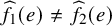$\widehat {f}_{1}(e) \neq \widehat {f}_{2}(e)$ . Thus,

since $\widetilde {\psi }_{\widehat {f}_{1}(e)}$ and $\widetilde {\psi }_{\widehat {f}_{2}(e)}$ are mutually orthogonal by the above observations.

Proposition 4.5. For each $\widehat {f}:\mathcal {E}_{\partial \mathcal {R}} \longrightarrow G$ , let us define

Recall that for each $a \in G$ , the element $\widehat {a}$ that appears on the right-hand side is the only choice compatible with $\widehat {f}$ and the fixed a. Then, $\mathcal {Q}_{\partial \mathcal {R}}(\widehat {f})$ is an orthogonal projection. Moreover, if $\widehat {f}_{1}$ and $\widehat {f}_{2}$ are different, then $\mathcal {Q}_{\partial \mathcal {R}}(\widehat {f}_{1})$ and $\mathcal {Q}_{\partial \mathcal {R}}(\widehat {f}_{2})$ are mutually orthogonal.

Proof. Let us first check that $\mathcal {Q}_{\partial \mathcal {R}}(\widehat {f})$ is an orthogonal projection. For that, it is enough to check that each of the two (tensor product) factors is a projection. The first factor is indeed a tensor product of projections $\frac {1}{|G|} \widetilde {\psi }_{g}$ . For the second factor, we just need to check that it is self-adjoint and idempotent. Since for every a, the adjoint of $\widetilde {\phi }_{a}$ is $\widetilde {\phi }_{a^{-1}}$ , it holds

and that the latter is, again, compatible with $\widehat {f}$ , since at each edge, the condition $a_{2} = g a_{1} g^{-1}$ is equivalent to $a_{2}^{-1} = g a_{1}^{-1} g^{-1}$ . Thus, summing over all $a \in G$ , we get self-adjointness, and so the first statement is proved. To see the second statement, note that

and that the resulting element $\widetilde {\phi }_{\widehat {ba}}$ is compatible with g, since $a_{2} = g a_{1} g^{-1}$ and $b_{2} = g b_{1} g^{-1}$ yield that $a_{2}b_{2} = g a_{1}b_{1} g^{-1}$ . Hence, summing over $a,b \in G$ in the previous expression, we get

This finishes the argument that $\mathcal {Q}_{\partial \mathcal {R}}(\widehat {f})$ is an orthogonal projection. Finally, if $\widehat {f}_{1}$ and $\widehat {f}_{2}$ are different, then we can check that $\mathcal {Q}_{\partial \mathcal {R}}(\widehat {f}_{1})$ and $\mathcal {Q}_{\partial \mathcal {R}}(\widehat {f}_{2})$ are mutually orthogonal, arguing as in the proof of Proposition 4.4.

Lemma 4.6. The operator

$$\begin{align*}\widetilde{\Delta} := \frac{1}{|G|} \sum_{g \in G}\widetilde{\psi}_{g} = \frac{1}{|G|} \sum_{g \in G}|{L^{g}}\rangle \langle{L^{g}}| \end{align*}$$

is a projection on $\ell _{2}(G) \otimes \ell _{2}(G)$ satisfying

Proof. It is clear from the above observations on $\frac {1}{|G|}\widetilde {\psi }_{g}$ that $\widetilde {\Delta }$ is actually the projection onto the vector subspace generated by vectors of the form $|{L^{g}}\rangle $ , and that $\widetilde {\Delta } \widetilde {\psi }_{g} = \widetilde {\psi }_{g} \widetilde {\Delta } = \widetilde {\psi }_{g} \,\,\, \text {for all } g \in G$ . To prove the last identity, let us apply (4.6) to decompose

$$\begin{align*}\begin{aligned} |{L^{g}}\rangle \langle{L^{g}}| = |{P_{1}}\rangle & \langle{P_{1}}| + |{P_{1}}\rangle \langle{\smash{P_{0} L^{g} P_{0}}}| + |{\smash{P_{0} L^{g} P_{0}}}\rangle \langle{P_{1}}| + |{\smash{P_{0} L^{g} P_{0}}}\rangle \langle{\smash{P_{0} L^{g} P_{0}}}| \,. \end{aligned} \end{align*}$$

Since $P_{1} = \frac {1}{|G|}\sum _{g \in G}{L^{g}}$ (see (4.5) and the subsequent discussion), we get after summing over $g \in G$ in the previous expression

$$\begin{align*}\widetilde{\Delta} = \frac{1}{|G|} \sum_{g \in G} |{L^{g}}\rangle \langle{L^{g}}| = |{P_{1}}\rangle \langle{P_{1}}| + \frac{1}{|G|} \sum_{g \in G} |{\smash{P_{0} L^{g} P_{0}}}\rangle \langle{\smash{P_{0} L^{g} P_{0}}}| \,.\end{align*}$$

Note that

that is $|{P_{1}}\rangle $ and $|{P_0L^{g}P_0}\rangle $ are both eigenvectors of

. As a consequence

and so taking adjoints, we immediately get that

This concludes the proof.

Proposition 4.7. The operator

is a projection on $\mathcal {H}_{\partial \mathcal {R}}$ satisfying

$$\begin{align*}\widetilde{\rho}_{\partial \mathcal{R}} = \widetilde{\rho}_{\partial \mathcal{R}} \, \widetilde{\mathcal{S}}_{\partial \mathcal{R}} = \widetilde{\mathcal{S}}_{\partial \mathcal{R}}\, \widetilde{\rho}_{\partial \mathcal{R}} \quad \quad , \quad \quad \mathcal{G}_{\partial \mathcal{R}} \, \widetilde{\mathcal{S}}_{\partial \mathcal{R}} = \widetilde{\mathcal{S}}_{\partial \mathcal{R}}\, \mathcal{G}_{\partial \mathcal{R}}. \end{align*}$$

Proof. The first statement is clear, as it is a tensor product of projections $\widetilde {\Delta }$ and $\widetilde {\phi }_{\widehat {1}}$ . Let us check that $\widetilde {\mathcal {S}}_{\partial \mathcal {R}} \, \widetilde {\rho }_{\partial \mathcal {R}} \, = \, \widetilde {\rho }_{\partial \mathcal {R}}$ . In view of the representation of $\widetilde {\rho }_{\partial \mathcal {R}}$ given in (4.19), it is enough to prove that

(4.22)

for all possible choices of $\widehat {g}$ and $\widehat {a}$ . The composition on the left-hand side of (4.22) is, again, a tensor product of operators of the form $\widetilde {\phi }_{1} \, \widetilde {\phi }_{a} = \widetilde {\phi }_{a}$ and $\widetilde {\Delta } \, \widetilde {\psi }_{g} = \widetilde {\psi }_{g}$ , so (4.22) holds. Analogously, we can argue that $\widetilde {\rho }_{\partial \mathcal {R}} \, \widetilde {\mathcal {S}}_{\partial \mathcal {R}} = \widetilde {\rho }_{\partial \mathcal {R}}$ .

Finally, to see that $\mathcal {G}_{\partial \mathcal {R}} \, \widetilde {\mathcal {S}}_{\partial \mathcal {R}} = \widetilde {\mathcal {S}}_{\partial \mathcal {R}}\, \mathcal {G}_{\partial \mathcal {R}}$ , note that both $\mathcal {G}_{\partial \mathcal {R}} $ and $\widetilde {\mathcal {S}}_{\partial \mathcal {R}}$ have a compatible tensor product structure, so that their product $\mathcal {G}_{\partial \mathcal {R}} \, \widetilde {\mathcal {S}}_{\partial \mathcal {R}}$ is, again, a tensor product of elements of the form

and analogously for $\widetilde {\mathcal {S}}_{\partial \mathcal {R}} \, \mathcal {G}_{\partial \mathcal {R}}$ ,

By Lemma 4.6, we know that

. For the others, we only need to check that

This finishes the proof.

Tool Box 2: Plaquette constants

We need a couple of auxiliary results. First, let us introduce the notation

$$\begin{align*}\widetilde{\chi}^{reg}(g) = \chi^{reg}(g) - 1 = |G| \delta_{g,1} - 1\,, \quad g \in G\,. \end{align*}$$

If $P_{1}$ is the projection onto $V_{1}$ , then

Lemma 4.8. Let us fix $u,v \in G$ and complex numbers $a_{0}, b_{0}, a_{1}, b_{1} \in \mathbb {C}$ . Then,

$$\begin{align*}\begin{aligned} \sum_{g_{1}, \ldots, g_{m} \in G} \left( a_{0} + b_{0} \, \widetilde{\chi}^{reg}(u g_{1} \ldots g_{m})\right) \, & \left( a_{1} + b_{1} \widetilde{\chi}^{reg}(g_{m}^{-1} \ldots g_{2}^{-1} g_{1}^{-1} v)\right) \\ &\quad\quad\quad = |G|^{m} \, \left( a_{0}a_{1} + b_{0} b_{1} \widetilde{\chi}^{reg}(uv) \right)\,. \end{aligned} \end{align*}$$

Proof. Note that the left-hand side of the equality can be rewritten as

$$\begin{align*}\begin{aligned} \sum_{g \in G} \,\, \sum_{\substack{g_{1}, \ldots, g_{m} \in G \\ g_{1} \, \ldots \, g_{m} =g}} \, & \left(a_{0} + b_{0} \widetilde{\chi}^{reg}(ug)\right) \, \left(a_{1} + b_{1} \widetilde{\chi}^{reg}(g^{-1}v)\right) \\ & \quad \quad = |G|^{m-1} \, \sum_{g \in G} \left(a_{0} + b_{0} \widetilde{\chi}^{reg}(ug)\right) \, \left(a_{1} + b_{1} \widetilde{\chi}^{reg}(g^{-1}v)\right) \end{aligned} ,\end{align*}$$

so we can restrict ourselves to the case $m=1$ . First, let us expand

The second and third summands are equal to zero, since

$$\begin{align*}\sum_{h \in G} \widetilde{\chi}^{reg}(h) = \sum_{h \in G} \left( |G| \, \delta_{h,1} -1 \right) = |G| - |G| = 0\,. \end{align*}$$

Moreover,

so the fourth summand in the aforementioned expansion is equal to $b_{0} b_{1} \widetilde {\chi }^{reg}(uv)$ , leading to the desired statement.

Next, we need a result which helps us to deal with the constants

$$\begin{align*}c_{\beta}( \, \widehat{g} \, ) \, := \, \prod_{ \substack{p \text{ inner}\\ \text{plaquette}} } \left( 1 + \gamma_{\beta} \, \chi^{reg}(\widehat{g}|_{p}) \, \right) \end{align*}$$

that appear in $\widetilde {\rho }_{\partial \mathcal {R}}$ , see (4.19). Let us first extend the notation $\chi ^{reg}(\widehat {g}|_{p})$ from plaquettes to the boundary of the rectangle $\mathcal {R}$ : let us enumerate its boundary edges $\mathcal {E}_{\partial \mathcal {R}}$ counterclockwise by fixing any initial edge $e_{1}, e_{2}, \ldots , e_{k}$ . Given a map $\widehat {f} : \mathcal {E}_{\partial \mathcal {R}} \longrightarrow G$ associating $e_{j} \longmapsto g_{j}$ , let us define

where $\sigma _{j} = 1$ if $e_{j}$ is in the upper or left side of the rectangle, and $\sigma _{j} = -1$ otherwise. We will also use the notation

$$\begin{align*}\widetilde{\chi}^{reg}(\widehat{f}) := \chi^{reg}(\widehat{f})-1\,. \end{align*}$$

As in the case of plaquettes, note that the definition is independent of the enumeration of the edges as long as it is done counterclockwise ( $\chi ^{reg}$ is invariant under cyclic permutations) and respects the inverses ( $\sigma _{j}=-1$ ) on the lower and right edges.

Proposition 4.9. For fixed $\widehat {f}: \mathcal {E}_{\partial \mathcal {R}} \longrightarrow G$ , we have that

$$\begin{align*}\sum_{\substack{\widehat{g}: \mathcal{E}_{\mathcal{R}} \longrightarrow G\\ \widehat{g}|_{\mathcal{E}_{\partial \mathcal{R}}} = \widehat{f} }} c_{\beta}(\widehat{g}) \,\, = \,\, |G|^{{|{\mathcal{E}_{\mathring{\mathcal{R}}}}|}} \, \left( \left(1 + \gamma_{\beta} \right)^{n_{\mathcal{R}}} + \gamma_{\beta}^{n_{\mathcal{R}}} \,\, \widetilde{\chi}^{reg}(\widehat{f}) \right)\,. \end{align*}$$

Proof. If the region $\mathcal {R}$ only consists of one plaquette, then the identity is trivial since there is only one summand $\widehat {g} = \widehat {f}$ , so that

$$\begin{align*}c_{\beta}(\widehat{g}) \, = \, 1 + \gamma_{\beta} \chi^{reg}(\widehat{g}|_{p}) = \left( 1 + \gamma_{\beta}\right) + \gamma_{\beta} \,\, \widetilde{\chi}^{reg}(\widehat{g}|_{p})\,. \end{align*}$$

Let us denote to simplify notation

$$\begin{align*}a_{\beta} := 1 + \gamma_{\beta} \quad , \quad b_{\beta}:= \gamma_{\beta}\,. \end{align*}$$

For multiplaquette rectangular regions, the key is Lemma 4.8. Let us illustrate the case of a region $\mathcal {R}$ consisting of two (adjacent) plaquettes.

Then, as a consequence of the aforementioned lemma

The procedure is now clear and can be formalized by induction. Let $\mathcal {R}$ be a rectangular region. We can obviously split $\mathcal {R}$ into two adjacent rectangles sharing one side $\mathcal {R}=AC$ as below. The induction hypothesis yields that the identity is true for A and C. Let us set some notation for the boundary edges of A and C:

Fix a boundary function $\widehat {f} : \mathcal {E}_{\partial \mathcal {R}} \rightarrow G$ (note that $\mathcal {E}_{\partial \mathcal {R}} = \alpha \gamma $ ), let us consider the sum over all choices $\widehat {g}: \mathcal {E}_{\mathcal {R}} \longrightarrow G$ , such that $\widehat {g}$ coincides with $\widehat {f}$ on the boundary edges of $\mathcal {R}$

(4.23)

Next, we want to apply the induction hypothesis on each subregion A and C. For that, we have to make the right expression appear. We can split the sum

(4.24)

Hence, we can rewrite (4.23) as

.

Applying the induction hypothesis, we have that the above expression can be rewritten as

where $n_{A}$ and $n_{C}$ are the number of inner plaquettes of A and C, respectively; $\widehat {g}|_{\alpha } \widehat {h}$ is the map $\mathcal {E}_{\partial A} \rightarrow G$ that coincides with $\widehat {g}$ on $\alpha $ and with $\widehat {h}$ on z; and $\widehat {h} \, \widehat {g}|_{\gamma }$ is the map $\mathcal {E}_{\partial C} \rightarrow G$ that coincides with $\widehat {g}$ on $\gamma $ and with $\widehat {h}$ on z. Finally, we use Lemma 4.8 to rewrite the above expression as

$$ \begin{align*} |G|^{|\mathcal{E}_{\mathring{A}}| + |\mathcal{E}_{\mathring{C}}| + |z|} \, \left( a_{\beta}^{n_{A} + n_{C}} + b_{\beta}^{n_{A} + n_{C}} \,\, \widetilde{\chi}^{reg}(\widehat{g}|_{\alpha} \widehat{g}|_{\gamma}) \right) \,. \end{align*} $$

Finally, observe that the set $\mathcal {E}_{\mathring {\mathcal {R}}}$ of inner edges of $\mathcal {R}$ is actually formed by the disjoint union of $\mathcal {E}_{\mathring {A}}$ , $\mathcal {E}_{\mathring {C}}$ and z, whereas the number $n_{\mathcal {R}}$ of inner plaquettes of $\mathcal {R}$ is indeed the sum of $n_{A}$ and $n_{C}$ , so that

$$\begin{align*}\sum_{\substack{\widehat{g}: \mathcal{E}_{\mathcal{R}} \rightarrow G \\ \widehat{g}|_{a \gamma} = \widehat{f}}} \, \prod_{\substack{p \subset \mathcal{R}\\ \text{plaquette}}} \left( a_{\beta} + b_{\beta} \,\, \widetilde{\chi}^{reg}(\widehat{g}|_{p}) \right) \,\, = \,\, |G|^{|\mathcal{E}_{\mathring{\mathcal{R}}}|} \, \left( a_{\beta}^{n_{\mathcal{R}}} + b_{\beta}^{n_{\mathcal{R}}} \,\, \widetilde{\chi}^{reg}(\widehat{f}) \right)\,. \end{align*}$$

This finishes the proof of the proposition.

Proof of the Leading term of the boundary Theorem 4.2

We are now ready to prove our main result about the boundary state of the thermofield double. Our starting point is (4.19). We can replace the sum over $\widehat {g}:\mathcal {E}_{\mathcal {R}} \rightarrow G$ with a double sum, the first one over $\widehat {f}: \mathcal {E}_{\partial \mathcal {R}} \rightarrow G$ (fixing first the values at the boundary), and the second one over 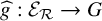$\widehat {g}:\mathcal {E}_{\mathcal {R}} \rightarrow G$ with $\widehat {g}|_{\mathcal {E}_{\partial \mathcal {R}}}=\widehat {f}$ , so that

where, from Proposition 4.9, it follows that

(4.25)

Let us now split the sum over $a \in G$ into a first summand with $a = 1$ (which forces $\widehat {a}(v) = 1$ for every $v \in \mathcal {V}_{\mathcal {R}}$ , as we argued in previous sections) and $a \neq 1$ :

In the first summand, we can, moreover, decompose

Thus, combining both expressions

Dividing the above expression by

$$\begin{align*}\kappa_{\mathcal{R}} = |G|^{{|{\mathcal{E}_{\mathcal{R}}}|}} \, (1+ \gamma_{\beta})^{{|{\mathcal{V}_{\mathring{\mathcal{R}}}}|} + n_{\mathcal{R}}} \, = \, |G|^{{|{\mathcal{E}_{\mathring{\mathcal{R}}}}|} + {|{\mathcal{E}_{\partial \mathcal{R}}}|}} \, (1+ \gamma_{\beta})^{{|{\mathcal{V}_{\mathring{\mathcal{R}}}}|} + n_{\mathcal{R}}} \,, \end{align*}$$

we obtain

(4.26) $$ \begin{align} \frac{1}{\kappa_{\mathcal{R}}} \widetilde{\rho}_{\partial \mathcal{R}} = \mathcal{S}_{1} + \left(\frac{\gamma_{\beta}}{1+\gamma_{\beta}}\right)^{n_{\mathcal{R}}} \, \mathcal{S}_{2} + \, \left(\frac{\gamma_{\beta}}{1+\gamma_{\beta}}\right)^{|\mathcal{V}_{\mathring{\mathcal{R}}}|} \, \mathcal{S}_{3} - \, \left(\frac{\gamma_{\beta}}{1+\gamma_{\beta}}\right)^{|\mathcal{V}_{\mathring{\mathcal{R}}}|} \, \mathcal{S}_{4} ,\end{align} $$

where

Note that the first summand actually corresponds to

To estimate the norm of $\mathcal {S}_{2}$ and $\mathcal {S}_{4}$ , we are going to use that the operators

are (orthogonal) projections and mutually orthogonal (see Proposition 4.4). Then, we can estimate

$$\begin{align*}\| \mathcal{S}_{2} \| \,\, \leq \,\, \sup_{\widehat{f}: \mathcal{E}_{\partial \mathcal{R}} \longrightarrow G} \,\,\, |\widetilde{\chi}^{\, reg}(\widehat{f} \,)| \leq |G|\,, \end{align*}$$

and by recalling that Proposition 4.9 implies the formula for $c_{\beta }(\widehat {f})$ given in (4.25), we obtain

$$ \begin{align*} \| \mathcal{S}_{4}\| \,\, \leq \,\, \sup_{\widehat{f}: \mathcal{E}_{\mathcal{R}} \longrightarrow G} \,\,\, \frac{c_{\beta}( \, \widehat{f} \, )}{(1+\gamma_{\beta})^{n_{\mathcal{R}}}\, |G|^{{|{\mathcal{E}_{\mathring{\mathcal{R}}}}|}}} \leq 1 + \left( \frac{\gamma_{\beta}}{1+\gamma_{\beta}}\right)^{n_{\mathcal{R}}} \, |G|\,. \end{align*} $$

To estimate the norm of $\mathcal {S}_{3}$ , we are going to use that the operators

are (orthogonal) projections and mutually orthogonal (see Proposition 4.5). Then, again, by using (4.25),

$$\begin{align*}\| \mathcal{S}_{3}\| = \sup_{\widehat{f}: \mathcal{E}_{\partial \mathcal{R}} \longrightarrow G} \,\, \frac{|G| \, c_{\beta}(\widehat{f})}{(1+\gamma_{\beta})^{n_{\mathcal{R}}} |G|^{{|{\mathcal{E}_{\mathring{\mathcal{R}}}}|}}} \, \leq \, |G|\, \left[1 + \left( \frac{\gamma_{\beta}}{1+ \gamma_{\beta}}\right)^{n_{\beta}}|G|\right] \,. \end{align*}$$

Combining all these estimates, we can reformulate (4.26) as

$$\begin{align*}\widetilde{\rho}_{\partial \mathcal{R}} \,\, = \,\, \kappa_{\mathcal{R}} \,\, \big( \, \widetilde{\mathcal{S}}_{\partial \mathcal{R}} \, + \, \widetilde{\mathcal{S}}_{\partial \mathcal{R}}^{rest} \, \big)\,, \end{align*}$$

where the observable $\widetilde {\mathcal {S}}_{\partial \mathcal {R}}^{rest}$ satisfies

having used in the second inequality that $ |\mathcal {V}_{\mathring {\mathcal {R}}}| \leq n_{\mathcal {R}}$ .

Proof of the approximate factorization of the boundary Theorem 4.3

Let us assume that $\epsilon _{\mathcal {R}} <1$ . By Proposition 4.7, we have that $\widetilde {S}_{\partial \mathcal {R}}$ is a projection satisfying $\widetilde {\rho }_{\partial \mathcal {R}} = \widetilde {\rho }_{\partial \mathcal {R}}\widetilde {S}_{\partial \mathcal {R}}= \widetilde {S}_{\partial \mathcal {R}} \widetilde {\rho }_{\partial \mathcal {R}}$ . Moreover, by Theorem 4.2

(4.27) $$ \begin{align} \left\| \kappa_{\mathcal{R}}^{-1} \, \widetilde{\rho}_{\partial \mathcal{R}} - \widetilde{S}_{\partial \mathcal{R}} \right\| \, = \, \| \widetilde{S}_{\partial \mathcal{R}}^{rest} \| \leq \epsilon_{\mathcal{R}} < 1 \,. \end{align} $$

These three properties yield that $\widetilde {S}_{\partial \mathcal {R}} = \widetilde {J}_{\partial \mathcal {R}}$ , as a consequence of the next general observation:

Let T be a self-adjoint operator on $\mathcal {H} \equiv \mathbb {C}^{d}$ , and $\Pi $ an orthogonal projection onto a subspace $W \subset \mathcal {H}$ , such that $T \, \Pi = \Pi \, T = T$ and $\| T- \Pi \| < 1$ . Then, $\Pi $ is the orthogonal projection onto $(\ker {T})^{\perp }$ . Indeed, since $T = \Pi T \Pi $ , we have that $(\ker {T})^{\perp }$ is contained in W. If they were different subspaces, then there would be a state $|{u}\rangle \in W$ with $T|{u}\rangle = 0$ . But then, $1 = \langle {u}|{u}\rangle = \langle {u}|{(\Pi -T)u}\rangle \leq \| T - \Pi \| < 1$ .

Next, observe that by Proposition 4.7

$$\begin{align*}[\mathcal{G}_{\partial \mathcal{R}}, \widetilde{J}_{\partial \mathcal{R}}] \, = \, [\mathcal{G}_{\partial \mathcal{R}}, \widetilde{S}_{\partial \mathcal{R}} ] \, = \, 0\,. \end{align*}$$

This yields that $\rho _{\partial \mathcal {R}}$ and $\widetilde {\rho }_{\partial \mathcal {R}}$ have the same support, that is $J_{\partial \mathcal {R}} = \widetilde {J}_{\partial \mathcal {R}}$ , since they are related via $\rho _{\partial \mathcal {R}} = \mathcal {G}_{\partial \mathcal {R}} \, \widetilde {\rho }_{\partial \mathcal {R}} \, \mathcal {G}_{\partial \mathcal {R}}$ , where $\mathcal {G}_{\partial \mathcal {R}}$ is invertible. Moreover, the operators $\sigma _{\partial \mathcal {R}} = \kappa _{\mathcal {R}} \, \mathcal {G}_{\partial \mathcal {R}} \, \widetilde {J}_{\mathcal {R}} \, \mathcal {G}_{\partial \mathcal {R}}$ and $\widetilde {\sigma }_{\partial \mathcal {R}} = \kappa _{\mathcal {R}}\, \widetilde {J}_{\mathcal {R}}$ will also have the same support as $\rho _{\partial \mathcal {R}}$ . We can thus argue as in the proof of Proposition 3.6 to get

$$ \begin{align*} \| \rho_{\partial \mathcal{R}}^{1/2} \, \sigma_{\partial \mathcal{R}}^{-1} \, \rho^{1/2}_{\partial \mathcal{R}} - J_{\partial \mathcal{R}} \| & = \| \widetilde{\rho}_{\partial \mathcal{R}}^{1/2} \, (\kappa_{\mathcal{R}} \widetilde{J}_{\partial \mathcal{R}})^{-1} \, \widetilde{\rho}^{1/2}_{\partial \mathcal{R}} - \widetilde{J}_{\partial \mathcal{R}} \|\\ & = \| \kappa_{\mathcal{R}}^{-1} \, \widetilde{\rho}_{\partial \mathcal{R}}^{1/2} \widetilde{J}_{\partial \mathcal{R}} \widetilde{\rho}_{\partial \mathcal{R}}^{1/2} - \widetilde{J}_{\partial \mathcal{R}} \| \\ & = \| \kappa_{\mathcal{R}}^{-1} \, \widetilde{\rho}_{\partial \mathcal{R}} - \widetilde{J}_{\partial \mathcal{R}} \|\, \leq \, \epsilon_{\mathcal{R}} ,\end{align*} $$

where in the last line, we have used, again, (4.27). Finally, since $\sigma _{\partial \mathcal {R}}$ and $\rho _{\partial \mathcal {R}}$ have the same support, we can use the identity

$$\begin{align*}\rho_{\partial \mathcal{R}}^{-1/2} \, \sigma_{\partial \mathcal{R}} \, \rho^{-1/2}_{\partial \mathcal{R}} = \big( \rho_{\partial \mathcal{R}}^{1/2} \, \sigma_{\partial \mathcal{R}}^{-1} \, \rho^{1/2}_{\partial \mathcal{R}} \big)^{-1} = J_{\partial \mathcal{R}} + \sum_{m=1}^{\infty} \,\big( J_{\partial \mathcal{R}} - \rho_{\partial \mathcal{R}}^{1/2} \, \sigma_{\partial \mathcal{R}}^{-1} \, \rho^{1/2}_{\partial \mathcal{R}}\big)^{m} \end{align*}$$

to deduce that

$$\begin{align*}\| \rho_{\partial \mathcal{R}}^{-1/2} \, \sigma_{\partial \mathcal{R}} \, \rho^{-1/2}_{\partial \mathcal{R}} - J_{\partial \mathcal{R}}\| \, \leq \, \sum_{m=1}^{\infty} \, \epsilon_{\mathcal{R}}^{m} = \frac{\epsilon_{\mathcal{R}}}{1-\epsilon_{\mathcal{R}}}\,. \end{align*}$$

4.4 Approximate factorization of the ground state projections

In this section, we study for a given rectangular region $\mathcal {R}$ split into three suitable regions $A, B, C$ , where B shields A from C and such that $AB, BC$ are again rectangular regions, how to estimate

$$\begin{align*}\| P_{ABC} - P_{AB} P_{BC}\| \end{align*}$$

in terms of the size of B. This problem is related to the approximate factorization property of the boundary states that we studied in the previous sections (see Section 3.4.2 for details on this relation and the main results in the context of general PEPS). Our main tools will be Theorems 3.5 and 4.3.

Corollary 4.10. Let us consider a rectangular region with open boundary conditions

split into three subregions $A,B,C$ , as in the next picture

so that $AB, BC, B$ are again rectangular regions. If B has M plaquettes per row and N plaquettes per column with

(4.28) $$ \begin{align} \epsilon_{B}:= 3 \, |G|^{2} \, \left( \frac{\gamma_{\beta}}{1+\gamma_{\beta}} \right)^{(M-1)(N-1)} \, < \, \frac{1}{2}\,, \end{align} $$

then the orthogonal projections $P_{\mathcal {R}}$ onto $\operatorname {Im}(V_{\mathcal {R}})$ satisfy

$$\begin{align*}\| P_{AB} P_{BC} - P_{ABC}\| \leq 16 \epsilon_{B} \,. \end{align*}$$

Proof. In order to apply Theorem 3.5, we arrange the virtual indices of $ABC$ , $AB$ , $BC$ , and B into four sets $a,c,\alpha , \gamma $ as in the next picture:

so that

$$\begin{align*}\partial ABC = ac \quad , \quad \partial AB = a \gamma \quad , \quad \partial BC = \alpha c \quad , \quad \partial B = \alpha \gamma\,. \end{align*}$$

The hypothesis $\epsilon _{B} < 1$ ensures that the hypothesis $\epsilon _{\mathcal {R}}<1$ in Theorem 4.3 is satisfied for $\mathcal {R} \in \{ B, AB, BC, ABC \}$ , and so $J_{\partial \mathcal {R}}$ and $\sigma _{\partial \mathcal {R}}$ have a simple tensor product structure. This allows us to factorize

where $J_{a}$ , $J_{c}$ , $J_{\alpha }$ , and $J_{\gamma }$ are projections. The local structure of $\widetilde {\mathcal {S}}_{\partial \mathcal {R}}$ and $\mathcal {G}_{\partial \mathcal {R}}$ allows us to decompose both operators as a tensor product of operators acting on $a,c,\alpha , \gamma $ . Hence, we can define

Then, we can easily verify that $\kappa _{ABC} \kappa _{B} = \kappa _{AB} \kappa _{BC}$ , and so

From Theorem 4.3, it follows that for each $\mathcal {R} \in \{ ABC, AB, BC, B\}$

$$\begin{align*}\| \rho_{\partial \mathcal{R}}^{1/2} \sigma_{\partial \mathcal{R}}^{-1} \rho_{\partial \mathcal{R}}^{1/2} - J_{\partial \mathcal{R}} \| < \epsilon_{B}\,, \end{align*}$$

and

$$\begin{align*}\| \rho_{\partial \mathcal{R}}^{-1/2} \, \sigma_{\partial \mathcal{R}} \, \rho_{\partial \mathcal{R}}^{-1/2} - J_{\partial \mathcal{R}} \| \, \leq \, \frac{\epsilon_{B}}{1-\epsilon_{B}} \leq 2 \epsilon_{B}\,.\end{align*}$$

Thus, applying Theorem 3.5, we conclude the result.

Analogously, we can prove results for the torus and cylinders.

Corollary 4.11. Let us consider a cylinder with open boundary conditions and split it into four sections $A,B,C,B'$ so that $B'AB$ and $BCB'$ are two overlapping rectangles whose intersection is formed by two disjoint rectangles B and $B'$ , as in the next picture:

Let us assume that B and $B'$ have at least M plaquettes per row and N plaquettes per column with

$$\begin{align*}\epsilon_{BB'}:= 3 \, |G|^{2} \, \left( \frac{\gamma_{\beta}}{1+\gamma_{\beta}} \right)^{(M-1)(N-1)} \, \leq \, \frac{1}{2}\,, \end{align*}$$

then the orthogonal projections $P_{\mathcal {R}}$ onto $\operatorname {Im}(V_{\mathcal {R}})$ satisfy

$$\begin{align*}\| P_{B'AB} P_{BCB'} - P_{ABCB'}\| \leq 48 \epsilon_{BB'} \,. \end{align*}$$

Proof. We are going to apply Theorem 3.5 for the three regions A, $BB'$ , and C. Firstly, we need to find a suitable arrangement of the virtual indices. First, we split the boundary of $BB'$ into two four parts $\gamma , \gamma ',\alpha , \alpha '$ as in

and define regions a and c according to

so that

$$ \begin{align*} & \partial B'AB=\gamma' a \gamma \quad , \quad \partial BCB' = \alpha c \alpha' \quad , \quad \partial ABCB' = ac\,,\\ & \partial B= \alpha \gamma \quad , \quad \partial B' = \gamma' \alpha'\,. \end{align*} $$

The local structure of $\widetilde {S}_{\partial \mathcal {R}}$ and $\mathcal {G}_{\partial \mathcal {R}}$ allows us to write them as a tensor product of operators acting on the defined boundary segments, and consider

Then, using that $\kappa _{ABC} \kappa _{B} \kappa _{B'} = \kappa _{B'AB} \kappa _{BCB'}$ , we can easily check that

By Theorem 4.3, we have for each $\mathcal {R} \in \{ B, B', B'AB, BCB', ABCB' \}$

$$ \begin{align*} \| \rho_{\partial \mathcal{R}}^{1/2} \sigma_{\partial \mathcal{R}}^{-1} \rho_{\partial \mathcal{R}}^{1/2} - J_{\partial \mathcal{R}} \| \,\, , \,\, \| \rho_{\partial \mathcal{R}}^{-1/2} \sigma_{\partial \mathcal{R}} \rho_{\partial \mathcal{R}}^{-1/2} - J_{\partial \mathcal{R}} \| \, \leq \, 2 \epsilon_{BB'} \,. \end{align*} $$

In particular, considering the joint region $BB'$ , we get

Applying Theorem 3.5, we conclude the result.

Corollary 4.12. We consider a decomposition of the torus into four regions $A,B,C,B'$ as below. We have then two overlapping cylinders $B'AB$ and $BCB'$ , whose intersection is formed by two disjoint cylinders B and $B'$ .

Let us assume that B and $B'$ have at least M plaquettes per row and N plaquettes per column with

$$\begin{align*}\epsilon_{BB'}:= 3 \, |G|^{2} \, \left( \frac{\gamma_{\beta}}{1+\gamma_{\beta}} \right)^{(M-1)(N-1)} \, \leq \, \frac{1}{2}\,, \end{align*}$$

then the orthogonal projections $P_{\mathcal {R}}$ onto $\operatorname {Im}(V_{\mathcal {R}})$ satisfy

$$\begin{align*}\| P_{B'AB} P_{BCB'} - P_{ABCB'}\| \leq 48 \epsilon_{BB'}\,. \end{align*}$$