


Introduction
The unending evolution of wireless communication networks demands highly efficient, compact, and broadband antennas for maximum data rates, minimum latency, and massive device networks [Reference Nasir, Jadoon, Owais, Iftikhar, Malik, Khan and Koziel1, Reference Çelik2]. One of the primary target bands for wireless deployment is the sub-8 GHz spectrum, particularly within the 4.5–8 GHz range, due to its favorable balance between coverage and capacity [Reference Çelik3, Reference Sen, Harutyunyan, Umar and Kamal4]. Among numerous varieties of antennas, Microstrip Patch Antennas (MPAs) are widely preferred for low-size design, simple fabrication, lightweight structure, and compatibility with integrated circuits. However, MPAs typically suffer from limitations such as narrow bandwidth and moderate gain, which restrict their standalone use in next-generation communication systems [Reference Yumuşak and Çelik5–Reference Douhi, Houssaini, Das, Subramanian, Madhav and Eddiai7]. Designing antennas that perform efficiently within this band while meeting modern wireless requirements presents unique challenges, such as bandwidth enhancement, gain improvement, and size reduction [Reference Khan, Ahmad and Alam8–Reference Dwivedi, Srivastava and Singh10]. A combination of advanced design techniques, innovative structural modifications, and strategic material selections is necessary to overcome these issues.
In the context of wireless transmission, particularly in the sub-8 GHz range, Multiple-Input Multiple-Output (MIMO) systems are vital for supporting high throughput, spatial diversity, and reliable signal transmission in complex environments [Reference Kim and Kong11]. MIMO antennas employ multiple radiating elements within a compact structure to enhance channel capacity and link robustness [Reference Khan, Song, Ullah, Qi, Zhang, Kamal, Shao, Gong, Khan, Livreri and Alibakhshikenari12]. However, a primary challenge in MIMO design is separation between the MIMO elements, minimizing the system performance, increases correlation, and reduces radiation efficiency [Reference Li, He, Zhou, Zhang and Wu13]. Effective mutual coupling reduction is crucial to maintain high isolation and optimize MIMO performance [Reference Elalaouy, El Ghzaoui and Foshi14]. Another promising enhancement technique involves the use of frequency-selective surface (FSS), periodic arrangements that reflect, transmit, or filter electromagnetic (EM) waves at different frequencies [Reference Cuiñas, Expósito, Andriukaitis, Caldeirinha, García Sánchez and Valinevičius15].
There has been much attention in the literature toward MIMO antenna design for sub-8 GHz applications, especially where efforts have been directed toward the development of high bandwidth, high isolation, and high-gain antennas. There have been some innovations in the area of MIMO MPAs. Nature-inspired geometry has been used to develop small 5G MPAs [Reference Nahar, Rawat, Pathak, Kumar and Anguera16], and a dual-band design based on complementary split-ring resonator configuration has been developed [Reference Chowdhury and Ranjan17]. In addition, large MIMO antenna arrays designed for sub-6 GHz have been made to achieve high gain and coverage [Reference El Ghaoual, Zbitou, Hefnawi and El Hammoumi18], along with compact multi-port antennas with good isolation properties [Reference Srinubabu and Rajasekhar19]. Additionally, passive decoupling techniques using resonator-based structures have been proposed to mitigate mutual coupling effects [Reference Singh, Tomar and Parihar20].
The manipulation of wave propagation in FSSs has received a great deal of attention in many research papers. Gain, directivity, and bandwidth have increased greatly after integrating these structures with antennas, while undesired frequency components and radiation modes have been eliminated [Reference Sharma and Kumar21]. These FSS structures act either as superstrates or ground plane modifications to achieve effective control over the antenna’s radiations [Reference Rajavel and Ghoshal22]. FSSs have been utilized in wideband and polarization-independent structures to shield against EM waves [Reference Chatterjee, Dey, Roy and Parui23, Reference Meka and Krishnan24] and in dual-band and optically transparent structures for communication applications [Reference Abdollahvand, Martinez-de-rioja, Katoch, Arboleya and Fontá25, Reference Nasir, Koziel and Iftikhar26]. Also, some work has been performed to enhance indoor transmissions of signals using FSS-based structures in the 5G environment [Reference Nguyen, Jung, Lee and Moon27].
It is also observed that the combination of FSS and MIMO antennas improves the gain and isolation of such antennas. The performance improvements are achieved through the use of FSS-backed or metasurface-assisted MIMO antennas, which include orthogonally configured radiating elements and FSS arrays [Reference Ud Din, Alibakhshikenari, Virdee, Ullah, Ullah, Akram, Ali, Livreri and Limiti28], compact designs with parasitic elements [Reference Zeain, Abu, Althuwayb, Alsariera, Al-gburi, Abdulbari and Zakaria29], and metamaterial enhancements [Reference Hasan, Islam, Alam, Kirawanich, Alamri and Alshammari30] and metasurface-based suppression of coupling effects [Reference Raza, Zhang and Yan31]. Also, there are reports of FSS superstrate spatial filtering antennas [Reference Li, Nie, Yang, Liu, Lin and Huang32].
There are some limitations associated with the existing MIMO-MPAs and FSS-assisted systems, including narrow bandwidth, low gain, high mutual coupling, and multilayered designs. Most designs have not covered the entire sub-8 GHz band and cannot be used for compact 5G and WLAN communication systems. Designing a system with high performance results in increased fabrication costs, especially when using FR4 substrates.
This work provides solutions by introducing new compact 2P and 4P MIMO-MPAs for sub-8 GHz bands that can support wide bandwidth, high gain, and reduced mutual coupling with an affordable and easy-to-fabricate design. The square-ring Defected Ground Structure (DGS) technique is adopted to increase bandwidth. On the other hand, orthogonal elements and a new coupling network scheme are used to minimize mutual coupling. The design is built on an FR4 substrate to achieve cost-effective and easy fabrication. Besides, a single-layer FSS with hybrid cells is integrated into the design to boost gain and directionality without impairing the impedance characteristics of the antenna. Some key contributions of this study are as follows:
• In contrast with previous studies where each parameter was optimized independently, this design is capable of delivering a broad bandwidth (4.69–8.1 GHz), low mutual coupling (envelope correlation coefficient [ECC] < 0.002), and improved gain at the same time.
• The approach of improving isolation performance by introducing a tilted cross-type coupling structure together with orthogonal positioning of antennas is used to effectively reduce mutual coupling without increasing the antenna’s physical dimensions.
• A single-layer FSS with a square/cross-slot hybrid cell structure is utilized to deliver 1–1.2 dB improvement in gain due to constructive interference effects, but without impairing impedance-matching properties of the designed system.
• The proposed antenna offers good performance with a very small physical size (∼0.63λ₀ × 0.63λ₀) in terms of multi-objective measures (diversity gain [DG] > 9.99 dB, channel capacity loss [CCL] < 0.03 bps/Hz, total active reflection coefficient [TARC] −13 dB).
The research is organized with section II for the proposed MIMO antenna, section III for the frequency-selective surface design, section IV shows the result analysis of the proposed antenna, section V includes the experimental outcomes, section VI includes a discussion, section VII concludes the research and also includes the future scope of the research.
Proposed MIMO antenna
The proposed MPA (PMPA) is designed using FR4 substrate ( $\varepsilon r = \,4.4\,,\,\delta = \,0.02$) with a thickness of 1.6 mm. The PMPA and the MIMO designs are implemented and analyzed using Ansys High-Frequency Structure Simulator (Ansys HFSS). Additionally, the research is conducted on a desktop with 32 GB RAM and Intel(R) Core (TM) i7-6700 CPU@3.40 GHz specifications.
Single-port antenna
The single-port antenna serves as the baseline design, from which the MIMO configurations are derived. The geometric layout is of a modified rectangular patch with few slots and parasitic structures to modify the operation as desired.
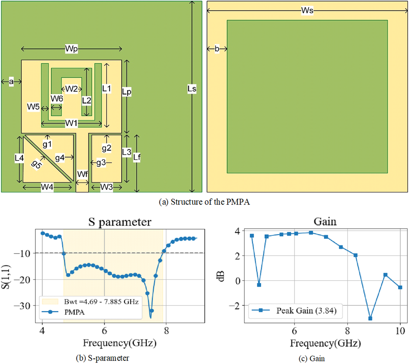
Figure 1(a) includes reflection coefficient (S11) vs. frequency plot, showing resonant frequencies and return loss. The S11 of the PMPA is <−10 dB with an operating band range of 3.195 GHz. Figure 1(b) includes a plot of gain across frequency where the gain improvements of PMPA indicate better radiation efficiency and directional performance. In Fig. 1(c), the Voltage Standing Wave Ratio (VSWR) vs. frequency is included, where VSWR < 2 indicates good impedance matching in the operating band.
Proposed PMPA (a) antenna geometry, (b) simulated reflection coefficient (S-parameters), and (c) realized gain characteristics.

Figure 1 Long description
The structure of the PMPA antenna with labeled dimensions including Wp, Lp, W1, L1, W2, L2, W3, L3, W4, L4, W5, L5, W6, L6, W7, L7, W8, L8 and G1 is shown in image A. The antenna is depicted with a central rectangular area surrounded by various sections and labeled lines indicating different widths and lengths. A plot of the S-parameter, specifically S11, against frequency in gigahertz is presented in image B. The plot shows a curve with a notable dip indicating a resonant frequency at approximately 7.985 gigahertz, where the S11 is less than minus 10 decibels, suggesting good performance. A gain plot against frequency in gigahertz is displayed in image C, showing variations in gain with a peak gain of 3.34 decibels. The gain plot indicates the antenna′s radiation efficiency and directional performance across the frequency range.
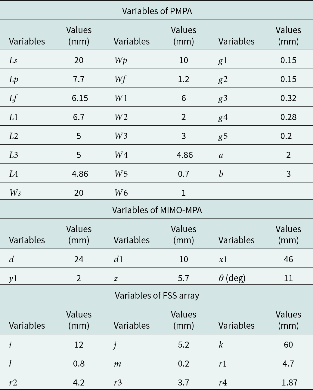
Table 1 contains all the design variables used throughout this research, including single-element antenna, 2P and 4P MIMO antennas, FSS unit cell, and FSS array.
Design dimensions of the PMPA, MIMO antenna, and FSS array

Table 1 Long description
Design dimensions in millimeters are provided for three components: a PMPA, a MIMO microstrip patch antenna, and an FSS array. PMPA values include multiple lengths and widths, with the largest listed dimensions at 20 mm for both a length and a width, and several small gap settings between 0.15 and 0.32 mm. Additional PMPA parameters include widths down to 0.7 mm and two feature sizes of 2 mm and 3 mm. MIMO antenna parameters include spacings and offsets such as 24 mm and 46 mm, plus smaller values like 2 mm and 5.7 mm, and one rotation angle of 11 degrees. FSS array parameters span from very small features at 0.2 mm and 0.8 mm up to a largest dimension of 60 mm, with four radius-like values between 1.87 mm and 4.7 mm. Overall, the table mixes fine fabrication-critical gaps with much larger layout dimensions, so units and parameter names should be matched carefully to the correct component section.
Patch and feed position
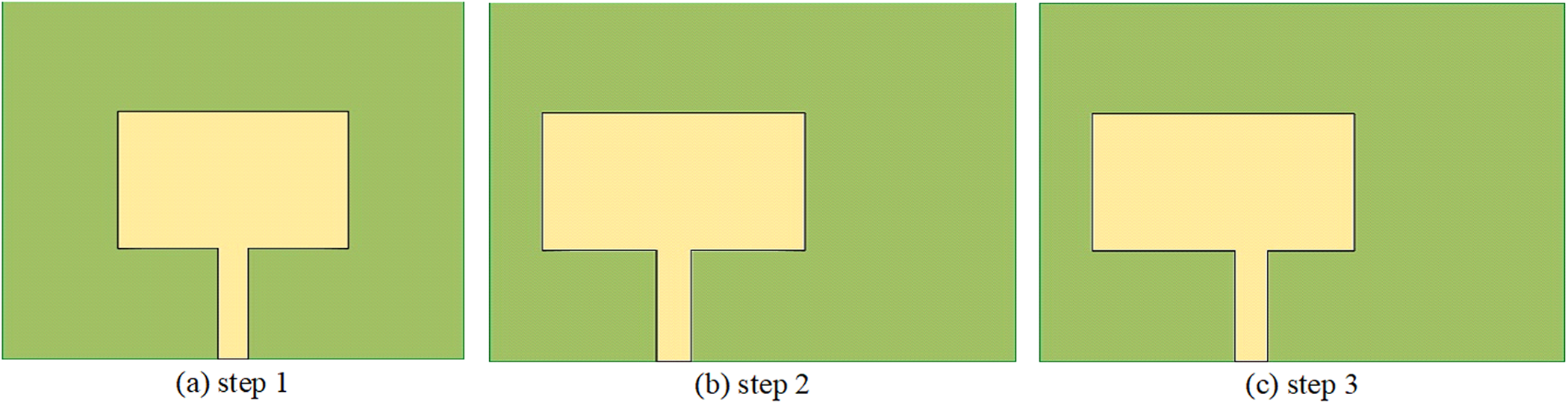
Typically, patch geometry is designed to achieve optimal resonance characteristics while maintaining compact dimensions. In this research, to maintain optimal spacing, the antenna is placed on the edge of the substrate to maintain maximum spacing on the other side. Additionally, feed placement plays a pivotal role in impedance matching and bandwidth tuning.
Figure 2(a) is the initial patch and feed configuration where the patch and feed are in the center position of the substrate. In Fig. 2(b), the patch and feed are shifted toward the left end of the substrate. In Fig. 2(c), the feed is shifted toward the right side of the patch. Each change influences impedance matching, resonant frequency, and radiation characteristics. Most importantly, these changes are done with the consideration of isolation and footprint as the antenna is developed into a MIMO antenna.
Evolution of the PMPA through different patch and feed configurations: (a) step 1, (b) step 2, and (c) step 3.

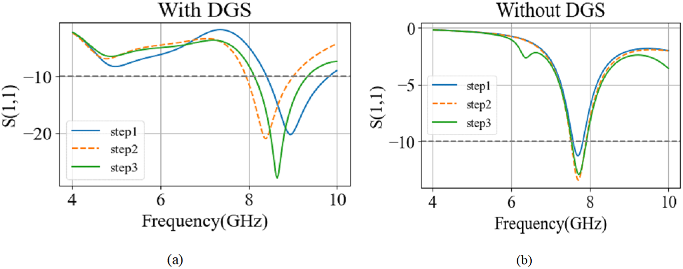
Figure 3(a, b) includes the performance effects of the patch and feed position with and without DGS. It is seen that DGS is necessary for the baseline antenna to obtain an optimal return loss and bandwidth. Additionally, step 3 provides optimal return loss when compared with the other two steps.
Influence of patch and feed positioning on antenna performance: (a) without DGS and (b) with DGS.

Design realization of the single-element patch antenna
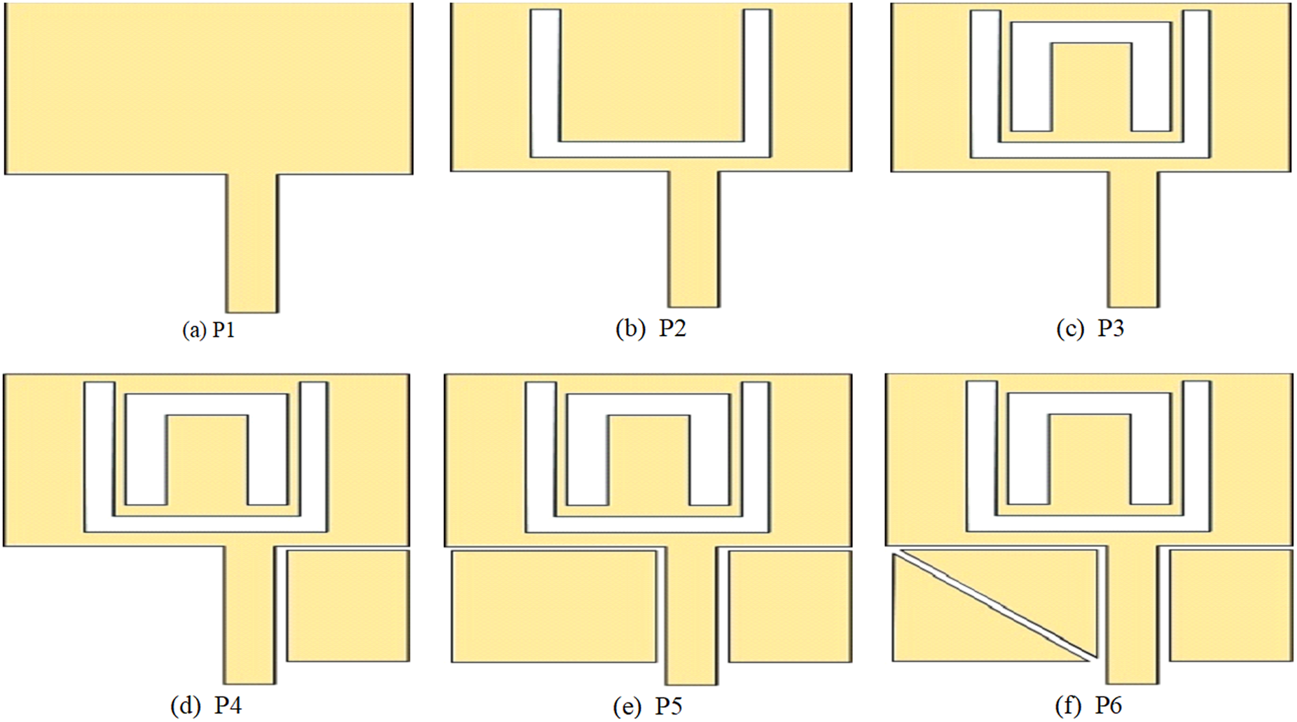
Figure 4(a–f) shows step-by-step modification of patch geometry, feed technique, and ground structure. These iterations demonstrate the development of PMPA to meet desired performance like wider bandwidth or better gain. P1 is a simple patch designed used as a baseline in this research. P2 includes a “U”-shaped slot, which introduces a different band at around 5 GHz, while P3 includes an additional inverted-“U”-shaped slot in an attempt to improve reflection coefficient and bandwidth. In P4, a parasitic structure is introduced, which improves the bandwidth of the antenna significantly, ranging approximately 2 GHz, however, with minimal return loss. P5 introduces a different parasitic structure that increases the return loss, while P6 improves the performance a step further to include optimal return loss and bandwidth.
Design evolution of the proposed PMPA: (a) initial structure (P1), (b) P2, (c) P3, (d) P4, (e) P5, and (f) final optimized design (P6).

Figure 4 Long description
The initial structure labeled P1, featuring a simple rectangular patch with a central feed line extending downward. P2, which introduces a U-shaped slot within the patch, altering the geometry to include a central cutout. P3, adding an inverted U-shaped slot inside the existing U-shaped slot, further modifying the patch geometry. P4, where a parasitic structure is added to the patch, consisting of additional rectangular sections on either side of the central feed line. P5, which includes a different parasitic structure, enhancing the complexity of the patch with more rectangular sections. The final optimized design labeled P6, featuring a diagonal line across the patch, indicating further refinement in the geometry. Each stage represents a step in the design evolution aimed at improving performance characteristics such as bandwidth and return loss.
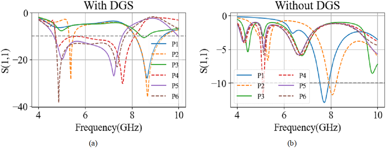
Figure 5(a, b) proves the need for the proposed DGS within the PMPA design to obtain optimal outcomes such as return loss and bandwidth. The full ground structure is highly reflective, while the DGS improves impedance matching or adds additional resonant modes to optimize the reflection coefficient and bandwidth of the PMPA.
Comparison of the simulated reflection coefficient (S11) of the PMPA: (a) without DGS and (b) with DGS.

Figure 5 Long description
Title text With DGS. Horizontal axis label: Frequency(GHz). Horizontal axis range: 4 to 10. Vertical axis label: S11. Vertical axis range: 0 to minus 40. Legend labels: P1, P2, P3, P4, P5, P6. Line style identification: P1 is a solid line. P2 is a dashed line. P3 is a dotted line. P4 is a dash dot line. P5 is a solid line. P6 is a dashed line. Data points as coordinate pairs. P1: (4, 0), (6, minus 20), (8, minus 10), (10, 0) P2: (4, 0), (6, minus 10), (8, minus 30), (10, 0) P3: (4, 0), (6, minus 15), (8, minus 5), (10, 0) P4: (4, 0), (6, minus 25), (8, minus 15), (10, 0) P5: (4, 0), (6, minus 5), (8, minus 20), (10, 0) P6: (4, 0), (6, minus 30), (8, minus 10), (10, 0) Lowest listed S11 values among the extracted points: P6 at (6, minus 30) and P2 at (8, minus 30). Title text Without DGS. Horizontal axis label: Frequency(GHz). Horizontal axis range: 4 to 10. Vertical axis label: S11. Vertical axis range: 0 to minus 40. Legend labels: P1, P2, P3, P4, P5, P6. Line style identification: P1 is a solid line. P2 is a dashed line. P3 is a dotted line. P4 is a dash dot line. P5 is a solid line. P6 is a dashed line. Data points as coordinate pairs. P1: (4, 0), (6, minus 10), (8, minus 20), (10, 0) P2: (4, 0), (6, minus 5), (8, minus 35), (10, 0) P3: (4, 0), (6, minus 15), (8, minus 10), (10, 0) P4: (4, 0), (6, minus 20), (8, minus 15), (10, 0) P5: (4, 0), (6, minus 10), (8, minus 25), (10, 0) P6: (4, 0), (6, minus 30), (8, minus 10), (10, 0) Lowest listed S11 value among the extracted points: P2 at (8, minus 35). Comparison using the extracted points: At Frequency 8, P2 is minus 30 in With DGS and minus 35 in Without DGS. At Frequency 6, P6 is minus 30 in both With DGS and Without DGS.
Defective ground plane
To overcome the limitations of conventional ground planes, a square-ring DGS is incorporated, significantly enhancing bandwidth and reducing surface-wave effects. Additionally, the dimensions and its influence on the PMPA’s performance are also analyzed.
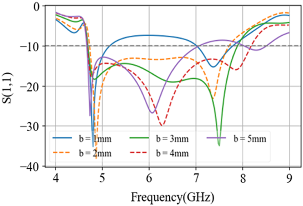
Figure 6 plots the effect of any changes in design parameter  $b$ (DGS) on the antenna’s reflection coefficient. According to the plot, PMPA operates optimally when
 $b = 3\,{\text{mm}}$. This plot shows that any changes in DGS affect PMPA’s bandwidth and reflection coefficient. Additionally, it might also affect the gain and isolation when built into a MIMO antenna.
Parametric analysis of the proposed PMPA illustrating the effects of antenna design parameters on the reflection coefficient.

Figure 6 Long description
The graph shows the reflection coefficient S(1,1) against Frequency in GHz. The horizontal axis is labeled Frequency(GHz) ranging from 4 to 9. The vertical axis is labeled S(1,1) ranging from 0 to minus 40. Five lines represent different b values: 1mm, 2mm, 3mm, 4mm and 5mm. Each line is visually distinguished by different styles: solid, dashed and dotted. Key observations include: the line for b equals 1mm shows a sharp dip around 5 GHz reaching approximately minus 30. The line for b equals 3mm shows a significant dip around 6.5 GHz reaching approximately minus 35. As b increases, the resonance dips shift slightly in frequency and depth. The graph illustrates how changes in b affect the reflection coefficient, with b equals 3mm showing the deepest dip, indicating optimal performance at this setting.
1 × 2 MIMO antenna
The transition from a single-port PMPA to a 2P-MIMO configuration introduces new challenges in reducing mutual coupling and optimizing spatial arrangement. The spacing arrangement maintained in the single-element design supports effectively achieving much space between the elements to reduce mutual interference.
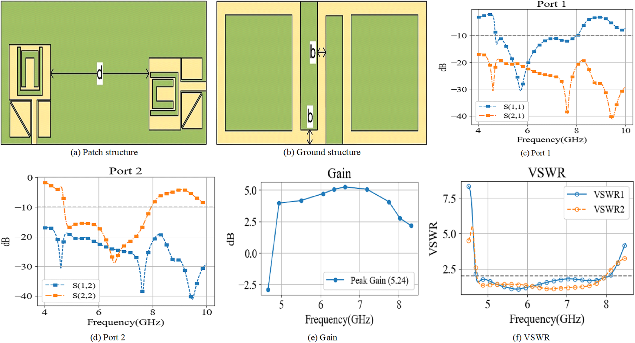
Figure 7(a, b) introduces patch and ground structures of proposed 2P-MIMO-MPA, placed in orthogonal configuration to reduce the spacing between elements. Figure 7(c, d) shows individual port responses to evaluate isolation and mutual coupling. It is seen that the isolation in both ports reaches almost 20 dB while maintaining a proper bandwidth and return loss. Figure 7(e, f) includes gain and VSWR of the proposed 2P-MIMO-MPA.
Configuration and simulated characteristics of the 2P-MIMO-MPA: (a, b) antenna geometry, (c, d) reflection coefficients of ports 1 and 2, (e) realized gain, and (f) VSWR.

Figure 7 Long description
Two rectangular layout drawings connected by a narrow line. The left drawing contains nested rectangular outlines and a small rectangular feature near the center. The right drawing contains a rectangular outline with a smaller rectangular feature inside and a diagonal line segment near the right side. Two large rectangular areas separated by a narrow vertical strip. Two small arrow markers point inward toward the central strip from left and right. The letter b appears near the arrows. Line graph titled Port 1. The x-axis is labeled Frequency(GHz), ranging from 4 to 10. The y-axis is labeled dB, ranging from minus 40 to 0. Two series are shown in the legend: S(1,1) and S(2,1). S(1,1) starts near about minus 2 at 4, drops to about minus 35 near 5, rises to about minus 10 near 6, rises to about minus 5 near 7, then stays between about minus 10 and minus 5 from 7 to 10. S(2,1) starts near about minus 10 at 4, drops to about minus 20 near 5, rises to about minus 10 near 6, then drops to about minus 35 near 9 and ends near about minus 20 at 10. Line graph titled Port 2. The x-axis is labeled Frequency(GHz), ranging from 4 to 10. The y-axis is labeled dB, ranging from minus 40 to 0. Two series are shown in the legend: S(1,2) and S(2,2). S(1,2) starts near about minus 5 at 4, drops to about minus 20 near 5, stays around minus 15 to minus 20 from about 5 to 7, rises to about minus 5 near 9 and ends near about minus 10 at 10. S(2,2) starts near about minus 10 at 4, drops to about minus 30 near 5, stays around minus 20 to minus 30 from about 5 to 8, drops to about minus 40 near 9.5 and ends near about minus 25 at 10. Line graph titled Gain. The x-axis is labeled Frequency(GHz), ranging from 4 to 8. The y-axis is labeled dB, ranging from minus 2.5 to 5.0. A single series is shown with a legend label Peak Gain (5.24). The curve rises from about minus 2.5 near 4 to about 4 near 5, increases to about 5 near 6, stays near about 5 from about 6 to 7, then decreases to about 2.5 near 8. Line graph titled VSWR. The x-axis is labeled Frequency(GHz), ranging from 4 to 8. The y-axis is labeled VSWR, ranging from 0 to 7.5. Two series are shown in the legend: VSWR1 and VSWR2. VSWR1 starts near about 7.5 at 4, drops to about 1 near 5, stays near about 1 from about 5 to 7, then rises to about 3 near 8. VSWR2 starts near about 5 at 4, drops to about 1 near 5, stays near about 1 from about 5 to 7, then rises to about 2.5 near 8.
S-shaped coupling structure in 1 × 2 MIMO antenna
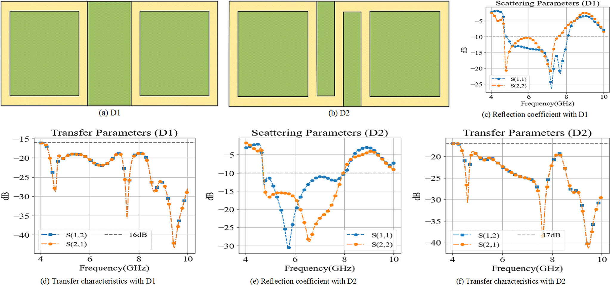
The 2P-MIMO-MPA achieves proper isolation, however, with space for improvement. As such, a novel S-shaped coupling structure is integrated into the ground plane to improve isolation and bandwidth, mitigating the adverse effects of close element placement.
Figure 8(a, b) represents physical layouts of two different DGS with and without coupling structures. As seen in Fig. 8(c, d), the return loss of 2P-MIMO-MPA is sub-optimal with acceptable isolation. An “S”-shaped coupling structure is introduced to lower the reflection coefficient and mutual coupling of the 2P-MIMO-MPA, as in Fig. 8(e, f).
Investigation of inter-element spacing in the proposed 2P-MIMO antenna: (a) spacing D1, (b) spacing D2, and corresponding (c–f) reflection and transmission characteristics.

Figure 8 Long description
Rectangular layout labeled (a) D1, with two large rectangular areas separated by a central vertical strip and a narrow border around the outer edge. Rectangular layout labeled (b) D2, with two large rectangular areas separated by a central vertical strip and a narrow border around the outer edge. Line graph titled Scattering Parameters (D1). The x-axis label is Frequency(GHz) with a range from 4 to 10. The y-axis label is dB with a range from 0 to negative 25. The legend lists S(1,1) and S(2,1). Two curves are plotted with point markers. The S(1,1) curve starts near 0 dB at 4, drops to a low point near 6, rises toward about 7, drops again near 8, then rises toward 10. The S(2,1) curve starts near 0 dB at 4, drops near 6, rises toward about 7, drops again near 8, then rises toward 10. Line graph titled Transfer Parameters (D1). The x-axis label is Frequency(GHz) with a range from 4 to 10. The y-axis label is dB with a range from negative 15 to negative 45. The legend lists S(1,2) and S(2,1). Two curves are plotted with point markers. Both curves start near negative 15 dB at 4, show a dip near about 4.5, rise toward about 6, show a deeper dip near about 7.5, rise near about 8, then drop again toward about 9.5 to 10. Line graph titled Scattering Parameters (D2). The x-axis label is Frequency(GHz) with a range from 4 to 10. The y-axis label is dB with a range from 0 to negative 30. The legend lists S(1,1) and S(2,1). Two curves are plotted with point markers. The S(1,1) curve starts near 0 dB at 4, drops to a deep low point near 6, then rises toward about 8 and remains near the upper part of the plotted range toward 10. The S(2,1) curve starts near 0 dB at 4, drops to a low point near about 6.5, then rises toward about 8 and remains near the upper part of the plotted range toward 10. Line graph titled Transfer Parameters (D2). The x-axis label is Frequency(GHz) with a range from 4 to 10. The y-axis label is dB with a range from negative 15 to negative 45. The legend lists S(1,2) and S(2,1). Two curves are plotted with point markers. Both curves start near negative 15 dB at 4, show a dip near about 4.5, rise toward about 6, show a deeper dip near about 7.5, rise near about 8, then drop again toward about 9.5 to 10.
2 × 2 MIMO antenna design
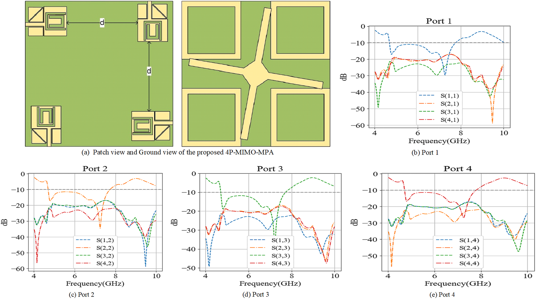
The design of 2P-MIMO-MPA is further developed into 4P-MIMO-PMPA to increase the channel capacity; however, it requires careful decoupling and impedance management. The 4P design also achieves much spacing between elements due to the design choice of PMPA, and it includes a coupling structure to improve isolation.
Figure 9(a) includes top and back designs of the proposed 4P-MIMO-MPA. As named, it is of four MPAs of distinct ports with a spacing of  $d$, while the ground planes are coupled using a cross-shaped coupler for optimal performance. Figure 9(b–e) includes S-parameters for each port separately to evaluate mutual coupling and matching, since high isolation among ports is critical for MIMO performance. Accordingly, the 4P MIMO antenna achieves isolation of at least >17 to ∼30 dB in every port within the specified operating range of the proposed MIMO-MPA.
Geometry and simulated reflection characteristics of the proposed 4-port MIMO microstrip patch antenna (4P-MIMO-MPA): (a) antenna structure and (b–e) reflection coefficients of ports 1–4.

Figure 9 Long description
The image includes the design and reflection characteristics of a four-port MIMO microstrip patch antenna. The left section shows the antenna′s patch and ground view, featuring four distinct microstrip patches with a cross-shaped coupler. The right section contains four graphs labeled Port 1 to Port 4, each displaying S-parameters over a frequency range from 4 to 10 GHz. Each graph has the x-axis labeled as Frequency in GHz and the y-axis as S-parameter magnitude in decibels. The graphs plot multiple traces, such as S11, S21, S31 and S41, indicating mutual coupling and matching for each port. Key observations include: Port 1 shows a main return-loss dip around 5 GHz with S11 reaching approximately -30 dB. Port 2 has a similar dip near 6 GHz. Port 3 and Port 4 show dips around 7 GHz. The coupling terms generally stay below -17 dB, indicating good isolation. The plots use different line styles to distinguish the traces, aiding in visual differentiation.
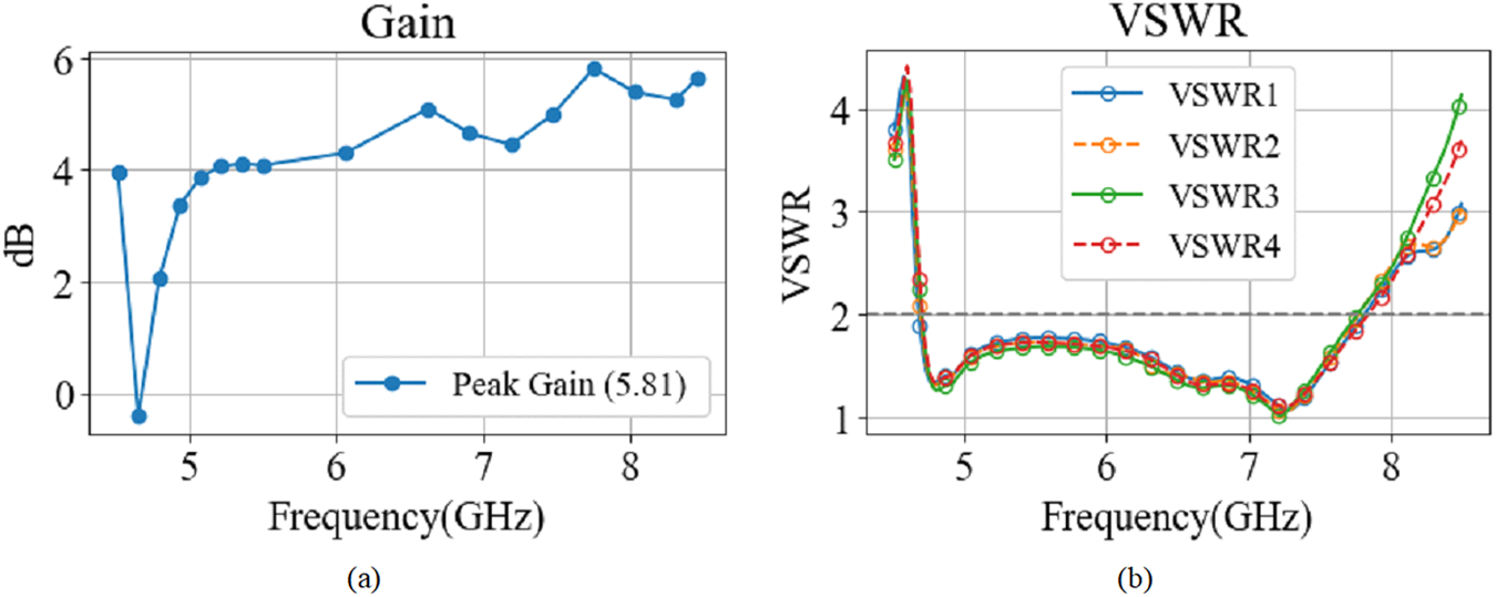
Figure 10(a, b) presents the gain and VSWR characteristics, proving that the proposed MIMO-MPA radiates efficiently while maintaining impedance consistency across all four elements. This balance between gain and impedance matching is crucial in real-time high-throughput systems where multiple antenna elements operate simultaneously. These results also imply minimal performance degradation due to mutual coupling, a typical challenge in MIMO design, for robust diversity and multiplexing performance.
Simulated radiation performance of the proposed 4P-MIMO-MPA: (a) realized gain and (b) VSWR.

Inclusion of coupling structure in the ground plane
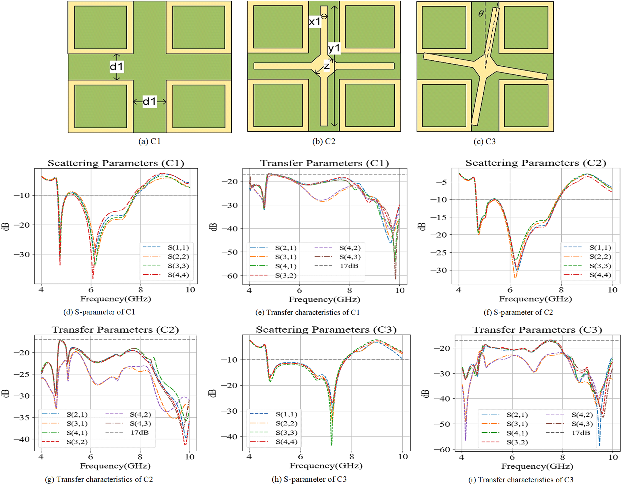
The effect of using the proposed coupling structure is also analyzed and compared with the 4P-MIMO-MPA without coupling structures. A cross-shaped meander-line coupling network is introduced in this research to reduce coupling between ports and maintain high isolation, ensuring robust MIMO performance.
Figure 11 explores the influence of different coupling structures (C1, C2, and C3) on the 4P-MIMO-MPA’s reflection coefficient and transfer characteristics. Figure 11(a–c) includes the evolution of coupling structures, where C1 is simply the ground planes without a coupling structure, while C2 contains a cross-shaped meander-line structure. In C3, the cross-shaped coupling structure is tilted to 11° to obtain optimal reflection characteristics and transfer characteristics. Figure 11(d–i) includes reflection coefficients and transfer characteristics of different coupling structures, where C1 shows moderate matching performance, with minimal bandwidth and isolation. C2 improves on isolation but is restricted in bandwidth, while C3 includes a balanced bandwidth and isolation.
Development of the decoupling/coupling structure: (a–c) design evolution and (d–i) corresponding reflection and transmission characteristics.

Figure 11 Long description
The composite figure contains nine panels labeled (a) through (i). Panels (a), (b) and (c) show the physical design layouts of coupling structures C1, C2 and C3 respectively. C1 shows a layout with ground planes and a dimension label d1. C2 shows a cross-shaped meander-line structure with labels x1, y1 and z. C3 shows the cross-shaped structure tilted at an angle with a label theta. Panel (d) is titled Scattering Parameters (C1). The horizontal axis shows frequency in gigahertz ranging from 4 to 10. The vertical axis shows magnitude in decibels. The legend lists S(1,1), S(2,2), S(3,3) and S(4,4). The curves show a notch at approximately 5.5 gigahertz reaching down to approximately negative 30 decibels. Panel (e) is titled Transfer Parameters (C1). The horizontal axis shows frequency in gigahertz from 4 to 10. The vertical axis shows magnitude in decibels. The legend lists S(2,1), S(3,1), S(4,1) and S(3,2), with a reference line at negative 17 decibels. The curves vary between approximately negative 20 and negative 60 decibels across the frequency range. Panel (f) is titled Scattering Parameters (C2). The horizontal axis shows frequency in gigahertz from 4 to 10. The vertical axis shows magnitude in decibels. The legend lists S(1,1), S(2,2), S(3,3) and S(4,4). The curves show a deeper notch compared to C1, reaching approximately negative 30 decibels near 5.5 gigahertz. Panel (g) is titled Transfer Parameters (C2). The horizontal axis shows frequency in gigahertz from 4 to 10. The vertical axis shows magnitude in decibels. The legend lists S(2,1), S(3,1), S(4,1) and S(4,3), with a reference line at negative 17 decibels. Curves show improved separation between transfer parameter values compared to C1, ranging between approximately negative 20 and negative 55 decibels. Panel (h) is titled Scattering Parameters (C3). The horizontal axis shows frequency in gigahertz from 4 to 10. The vertical axis shows magnitude in decibels ranging from approximately negative 5 to negative 45. The legend lists S(1,1), S(2,2), S(3,3) and S(4,4). The notch reaches approximately negative 40 decibels near 5.8 gigahertz, showing a wider and deeper response compared to C1 and C2. Panel (i) is titled Transfer Parameters (C3). The horizontal axis shows frequency in gigahertz from 4 to 10. The vertical axis shows magnitude in decibels. The legend lists S(2,1), S(3,1), S(4,1) and S(4,3), with a reference line at negative 17 decibels. Curves show values ranging between approximately negative 20 and negative 55 decibels, with more consistent separation across the frequency band compared to C1 and C2.
Performance comparison of the proposed 2P and 4P MIMO antennas
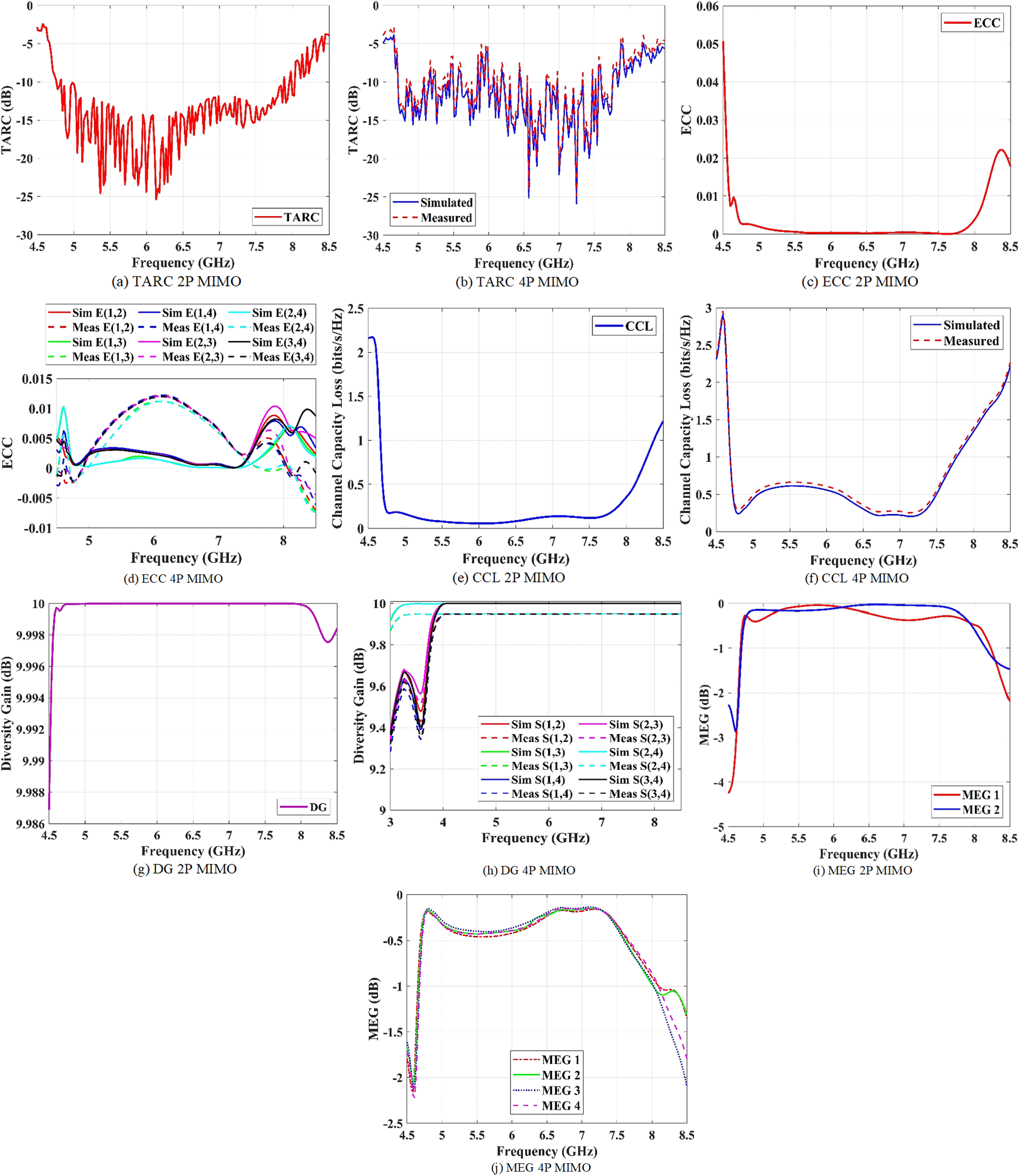
The progressive improvement in MIMO-MPA is measured using specific parameters like total ECC, TARC, CCL, DG, and mean effective gain (MEG).
Figure 12(a–j) includes various MIMO parameters across both 2P and 4P MIMO designs. The 4P MIMO offers superior DG and MEG, while the 2P shows higher ECC and TARC. Additionally, both the MIMO designs achieve ECC < 0.002 and DG > 9.9, which is significant in measuring the performance of the MIMO antennas.
(a–j) Comparison of key MIMO performance metrics for the proposed 2-port and 4-port antennas, including (a, b) TARC, (c, d) ECC, (e, f) CCL, (g, h) DG, and (i, j) MEG.

Figure 12 Long description
Line graph with the x-axis labeled Frequency (GHz) and the y-axis labeled TARC (dB). The x-axis ranges from 4.5 to 8.5. The y-axis ranges from negative 30 to 0. One curve is labeled TARC. The curve starts near negative 5 at 4.5, drops to around negative 25 between about 5.2 and 6.2, rises to around negative 15 near 6.8 and rises toward about negative 5 by 8.5. Line graph with the x-axis labeled Frequency (GHz) and the y-axis labeled TARC (dB). The x-axis ranges from 4.5 to 8.5. The y-axis ranges from negative 30 to 0. A legend lists Simulated and Measured. Two curves follow similar paths, starting near negative 5 at 4.5, dipping to around negative 20 to negative 25 between about 6.0 and 7.2 and rising toward about negative 5 by 8.5. Line graph with the x-axis labeled Frequency (GHz) and the y-axis labeled ECC. The x-axis ranges from 4.5 to 8.5. The y-axis ranges from 0.00 to 0.06. One curve is labeled ECC. The curve is near 0.06 at 4.5, drops close to 0.00 by about 4.8, stays near 0.00 through most of the mid-band, then rises to about 0.02 near 8.5. Line graph with the x-axis labeled Frequency (GHz) and the y-axis labeled ECC. The x-axis ranges from 4.5 to 8.5. The y-axis ranges from negative 0.01 to 0.015. A legend lists multiple traces labeled Sim E1,1, Sim E1,2, Sim E1,3, Sim E1,4, Sim E2,3, Sim E2,4, Sim E3,4 and corresponding Meas traces. Multiple curves cluster near 0.00 to 0.01 across the band, with several peaks around 5.0 to 5.5 and again around 7.8 to 8.5 and some segments dipping slightly below 0.00. Line graph with the x-axis labeled Frequency (GHz) and the y-axis labeled Channel Capacity Loss (bits per second per hertz). The x-axis ranges from 4.5 to 8.5. The y-axis ranges from 0.0 to 2.5. One curve is labeled CCL. The curve stays near 0.0 from 4.5 to about 7.0, then rises gradually and reaches about 1.0 to 1.2 near 8.5. Line graph with the x-axis labeled Frequency (GHz) and the y-axis labeled Channel Capacity Loss (bits per second per hertz). The x-axis ranges from 4.5 to 8.5. The y-axis ranges from 0.0 to 2.5. A legend lists Simulated and Measured. Two curves track closely, staying near 0.0 from 4.5 to about 7.0, then rising and reaching about 1.8 to 2.0 near 8.5. Line graph with the x-axis labeled Frequency (GHz) and the y-axis labeled Diversity Gain (dB). The x-axis ranges from 4.5 to 8.5. The y-axis ranges from 9.984 to 10.000. One curve is labeled DG. The curve stays close to 10.000 across most of the band, with a small drop near the upper end around 8.3 to 8.5. Line graph with the x-axis labeled Frequency (GHz) and the y-axis labeled Diversity Gain (dB). The x-axis ranges from 4.5 to 8.5. The y-axis ranges from 9.3 to 10.0. A legend lists multiple traces labeled Sim S1,1, Sim S1,2, Sim S1,3, Sim S1,4, Sim S2,2, Sim S2,3, Sim S2,4, Sim S3,3, Sim S3,4, Sim S4,4. Multiple curves rise steeply from about 9.3 near 4.5 to near 10.0 by about 5.0, then remain near 10.0 through about 8.5. Line graph with the x-axis labeled Frequency (GHz) and the y-axis labeled MEG (dB). The x-axis ranges from 4.5 to 8.5. The y-axis ranges from negative 4 to 0. A legend lists MEG 1 and MEG 2. Two curves stay near 0 from about 4.8 to about 7.8, then drop toward about negative 2 to negative 3 near 8.5. Line graph with the x-axis labeled Frequency (GHz) and the y-axis labeled MEG (dB). The x-axis ranges from 4.5 to 8.5. The y-axis ranges from negative 2.5 to 0. A legend lists MEG 1, MEG 2, MEG 3, MEG 4. Four curves stay near 0 from about 4.8 to about 7.6, then drop between about 7.8 and 8.5, reaching roughly negative 1.0 to negative 2.0 by 8.5, with the curves separating near the upper end.
FSS design
The gain and directivity of the MIMO-MPA are improved with the inclusion of proposed FSS (PFSS). In this research, a  $5\, \times \,5$ FSS array is designed on a Rogers RT/Duroid 5880 substrate (
 $\varepsilon r = \,2.2\,,\,\delta = \,0.0009$), and its performance evaluation establishes its role in improving antenna gain and directivity.
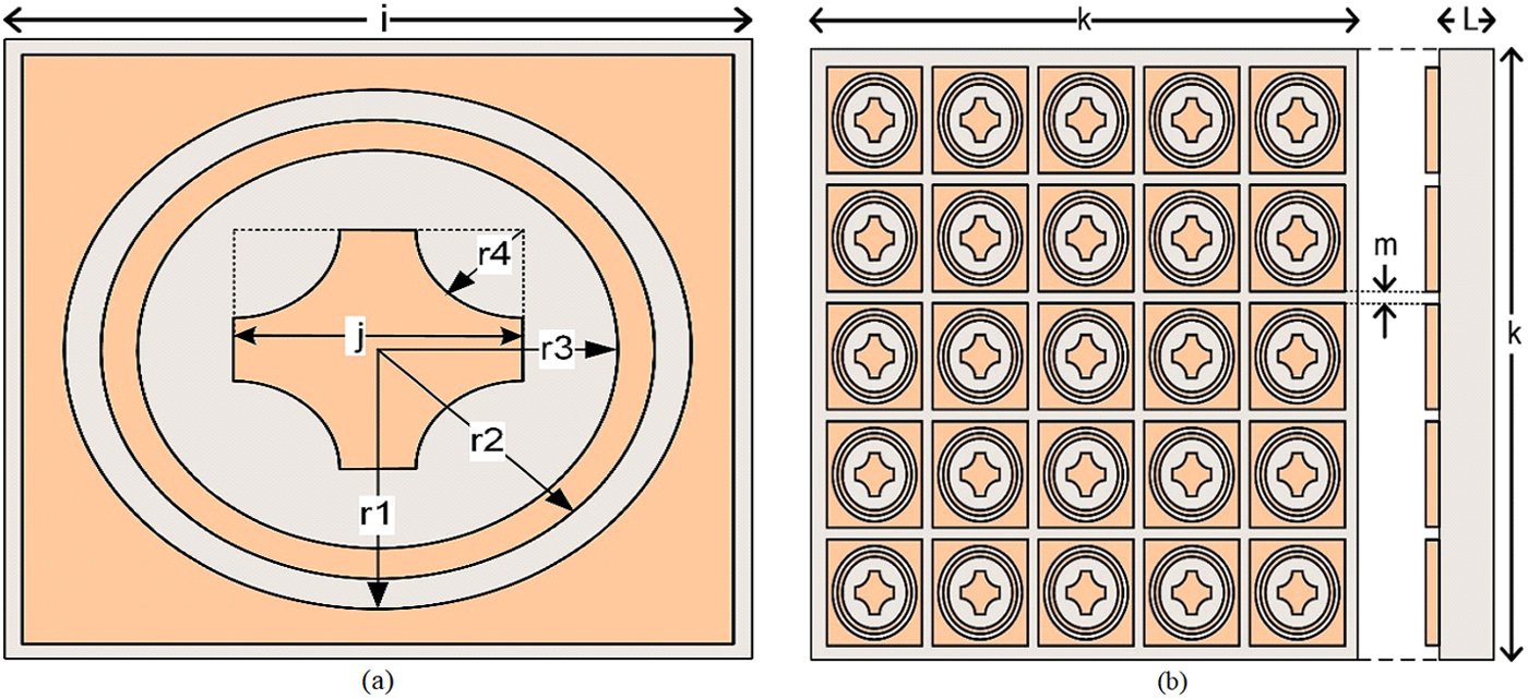
Figure 13(a, b) presents the structure of PFSS, highlighting the unit-cell configuration and its array configuration. The design integrates square unit cells with a circular slot, an inner ring, and a cross-structure to achieve the desired frequency response.
Proposed FSS: (a) unit-cell geometry and (b) front and side views of the periodic FSS array.

Figure 13 Long description
Parameterized unit cell for a frequency selective surface, drawn inside a square boundary with a concentric circular ring near the perimeter and a second concentric circular ring closer to the center. A central square sits inside the inner ring and a cross shaped feature spans across the central square with one horizontal bar and one vertical bar. Four dimension arrows are drawn on the geometry and labeled r1, r2, r3 and r4, with each label placed next to its arrow; no numeric values or units are printed next to these labels. Periodic layout of the same unit cell repeated in a square grid, with each cell containing the concentric ring and central cross pattern. Above the grid, a horizontal dimension line is labeled L. To the right of the grid, a narrow vertical side view is drawn as a tall rectangle with a vertical dimension line labeled k and a shorter vertical dimension line near the top labeled m; no numeric values or units are printed next to L, k, or m.
Physical mechanism of gain enhancement
The suggested FSS behaves as a partially reflective surface (PRS) positioned above the antenna at an optimal height, constituting the Fabry–Perot resonator. Once the antenna radiates, the EM waves are partly reflected from the FSS, and the rest of them are transmitted. Interaction between the reflected and directly radiated waves leads to their in-phase superposition in the broadside direction, causing constructive interference. In turn, the constructive interference results in an improvement of the directivity coefficient and an increase in the realized gain of the antenna without enlarging its size or applying additional input power. Moreover, by affecting the pattern of the antenna, the FSS redistributes energy into desirable directions, thus limiting undesirable emissions. The periodicity of the FSS structure also contributes to the suppression of the surface waves and back radiation, improving the radiation efficiency and front-to-back ratio. At the same time, the proper arrangement of the FSS provides optimal impedance characteristics of the antenna with respect to the minimum variation of VSWR values.
Unit-cell-level performance
Unit cells make up the core of the PFSS, providing both simplicity and wideband capability. The performance of the PFSS array can be analyzed by examining just one of its unit cells.
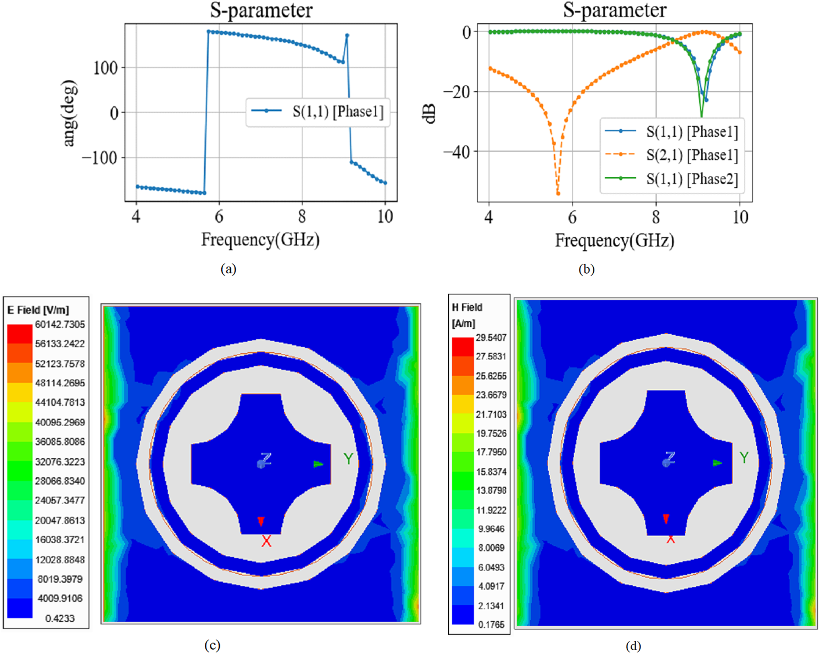
Figure 14(a–d) illustrates the frequency response of the unit cell of the FSS, showing how it reflects and transmits signals within the specified bandwidth. The steep variations in the S-parameter graphs indicate that the design can reject unwanted frequencies but pass the wanted frequencies.
Electromagnetic characteristics of the proposed FSS unit cell: (a) reflection phase, (b) transmission magnitude, (c) electric-field distribution, and (d) magnetic-field distribution.

Figure 14 Long description
A: Line plot titled S-parameter. The plot shows reflection phase versus frequency. The horizontal axis is labeled Frequency(GHz) with tick labels 4, 6, 8, 10. The vertical axis is labeled Phase(deg) with tick labels 0, 50, 100, 150. The legend shows S(1,1) [Phase]. The curve is near 0 from about 4 to 6, then rises to about 150 just after 6, stays near 150 until about 9, then drops to about 50 near 9.5 and approaches about 0 by 10. B: Line plot titled S-parameter. The plot shows magnitude in decibel versus frequency for multiple S-parameter traces. The horizontal axis is labeled Frequency(GHz) with tick labels 4, 6, 8, 10. The vertical axis is labeled dB with tick labels 0, minus 20, minus 40. The legend shows S(1,1) [Phase], S(2,1) [Phase] and S(1,1) [Phase2]. One curve forms a deep notch reaching about minus 40 at about 6, then rises toward 0 by about 10. The other two curves stay near 0 over most of the range, with a narrow dip near about 9 to 10 where one curve drops to roughly minus 20 to minus 30 before returning toward 0. C: Electric-field distribution map with a color scale labeled E Field (V/m). The scale ranges from 0.41735 to 84012.736. The map shows a ring-shaped structure around a central shape. Axis markers labeled x, y and z appear near the center. D: Magnetic-field distribution map with a color scale labeled H Field (A/m). The scale ranges from 1.7186 to 38.947. The map shows a ring-shaped structure around a central shape. Axis markers labeled x, y and z appear near the center.
EM behavior and operating principle of PFSS
To further understand the proposed PFSS structure, its EM characteristics are investigated through both magnitude and phase responses. From the results obtained using S-parameters, it is clear that the PFSS structure shows a band-pass response for the 6–8 GHz band, which can let the desired wave pass but block out the unwanted parts of the wave. Apart from the magnitude response, another parameter that should be considered in analyzing the operation of the proposed surface is the reflection phase response, since it helps confirm the functioning mode of the surface. The reflection phase of the surface does not stay around 0°; thus, it is evident that the proposed surface is not working as Artificial Magnetic Conductor (AMC). Rather, it works as a PRS. By optimizing the air gap distance, the PFSS acts like a Fabry–Perot type resonator, and the constructive interference helps improve gain and directivity.
Performance of FSS array
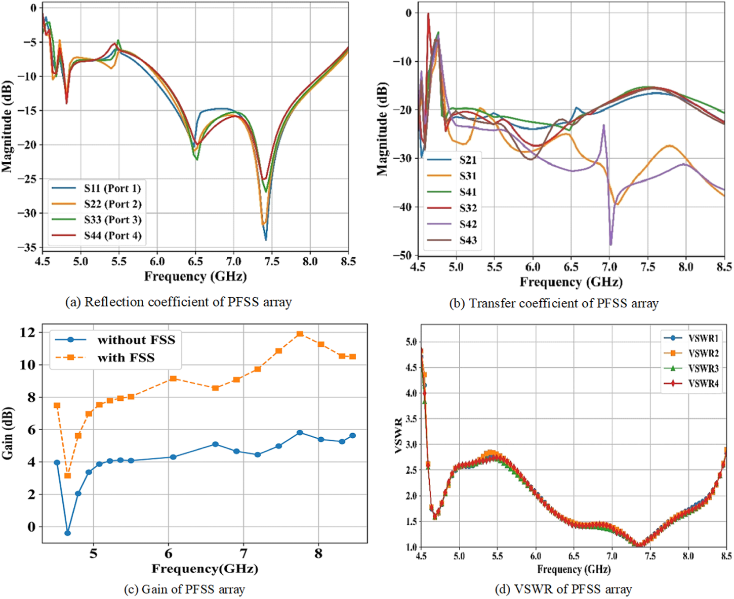
The unit cells are placed together periodically to form a finite-element array. This is to optimize the integration of PFSS with the 4P-MIMO-MPA. In this research, the reflection coefficient, transfer coefficient, and gain levels of the 4P-MIMO-MPA are analyzed along with the VSWR of the 4P-MIMO-MPA before and after the inclusion of PFSS. The air gap between the 4P-MIMO-MPA and PFSS is about 15 mm.
Figure 15(a–d) demonstrates the impact of the PFSS integrated with the 4P-MIMO-MPA, in reflection coefficient, transmission response, gain performance, and VSWR. The results reveal a noticeable gain enhancement, validating the PFSS’s role as a passive superstrate in boosting antenna directivity. The addition of PFSS improves the gain from an average of 5.81–11.91 dB. Additionally, the VSWR plot validates the impedance matching of the 4P-MIMO-MPA.
Performance of the FSS-integrated 4P-MIMO-MPA: (a) reflection coefficient, (b) transmission coefficient, (c) realized gain, and (d) VSWR.

Figure 15 Long description
Line graph with the horizontal axis labeled Frequency (GHz) and the vertical axis labeled Magnitude (dB). The frequency axis runs from 4.5 to 8.5. The magnitude axis runs from 0 to negative 40. A legend lists S11 (Port 1), S22 (Port 2), S33 (Port 3) and S44 (Port 4). The plotted curves show a dip near about 4.8, another dip near about 6.6 and a deeper dip near about 7.5. Line graph with the horizontal axis labeled Frequency (GHz) and the vertical axis labeled Magnitude (dB). The frequency axis runs from 4.5 to 8.5. The magnitude axis runs from 0 to negative 40. A legend lists S21, S31, S41, S32, S42 and S43. The plotted curves include a sharp feature near about 4.6 to 4.8, then values mostly between about negative 10 and negative 35 across the remaining frequency range, with several curves crossing each other. Line graph with the horizontal axis labeled Frequency (GHz) and the vertical axis labeled Gain (dB). The frequency axis runs from 4.5 to 8.5. The gain axis runs from 0 to 12. A legend lists without FSS and with FSS. The without FSS curve starts near about 0 around 4.7, rises to about 5 by about 5.0 and stays around about 5 to 7 through about 8.5. The with FSS curve starts near about 3 around 4.7, rises to about 8 by about 5.0, increases to about 12 near about 7.6, then decreases to about 10 by about 8.5. Line graph with the horizontal axis labeled Frequency (GHz) and the vertical axis labeled VSWR. The frequency axis runs from 4.5 to 8.5. The VSWR axis runs from 0 to 5. A legend lists VSWR1, VSWR2, VSWR3 and VSWR4. The curves are closely grouped, with values near about 5 around 4.5, dropping to around about 2 near about 5.0, reaching a low near about 1 around about 7.4 to 7.6, then rising toward about 3 to 4 by about 8.5.
Comparative analysis of various FSS
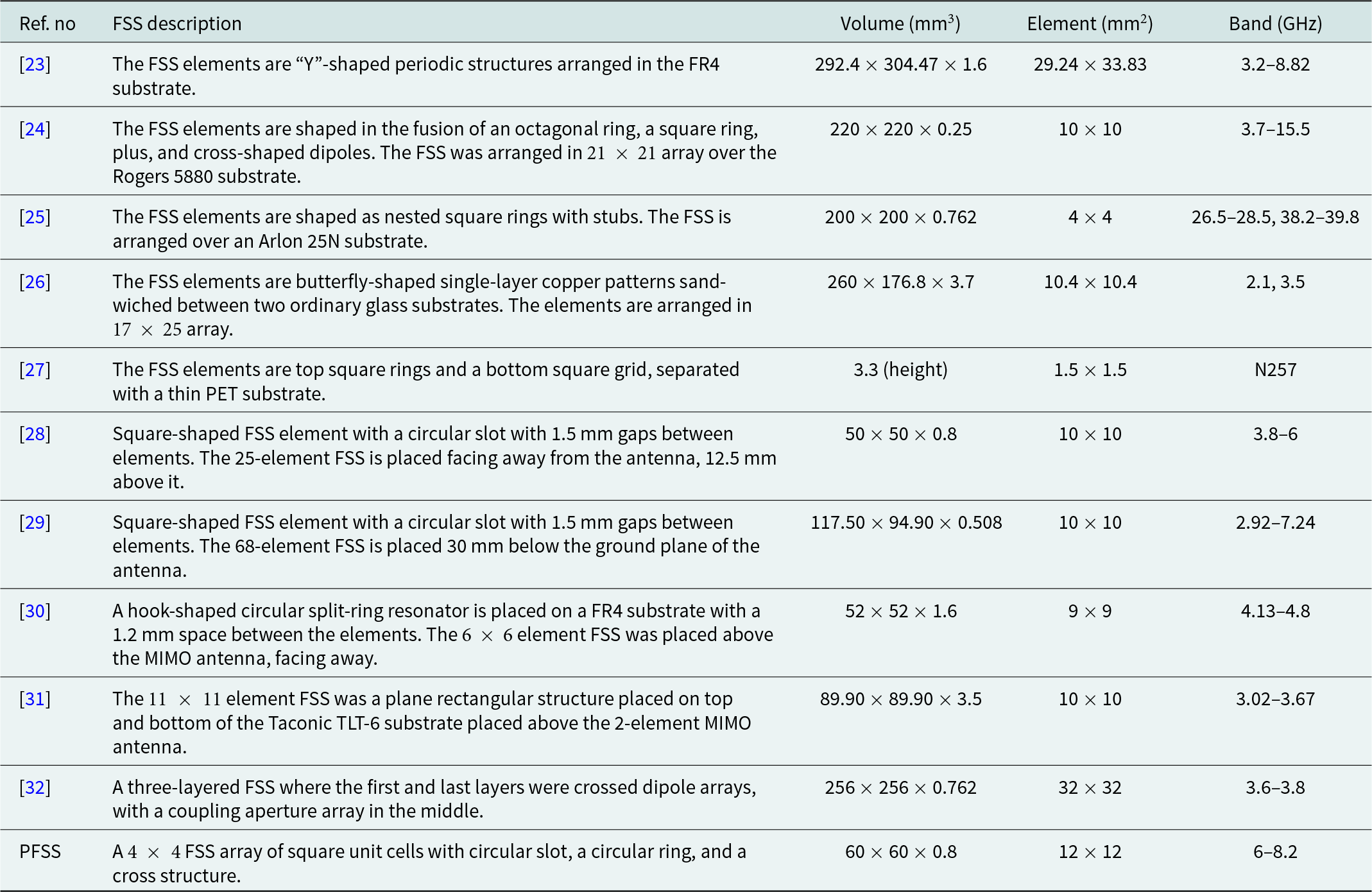
The impact of the PFSS on the overall antenna performance is compared with the literature in terms of volume and operational bandwidth. The literature [Reference Chatterjee, Dey, Roy and Parui23–Reference Li, Nie, Yang, Liu, Lin and Huang32] includes FSS and is used in this comparison.
Table 2 compares PFSS configurations across various literature employing a hybrid square–circular–cross-shaped unit cell, providing wideband operation in the sub-8 GHz range. Compared to [Reference Hasan, Islam, Alam, Kirawanich, Alamri and Alshammari30] and [Reference Raza, Zhang and Yan31], which target narrower or lower-frequency bands, the PFSS covers a broader range while maintaining a compact form factor. Unlike multilayered or bulky FSS designs such as [Reference Li, Nie, Yang, Liu, Lin and Huang32], which complicate integration, the PFSS remains single-layered and lightweight, ensuring compatibility with the proposed MIMO antennas without structural complexity, making it a viable enhancement for sub-8 GHz MIMO antennas.
Comparison of the proposed FSS with existing state-of-the-art FSS structures in terms of geometry, physical dimensions, unit-cell size, and operating frequency range

Table 2 Long description
Frequency selective surface designs are compared by element geometry, overall physical size (length, width, thickness), unit-cell size, and operating band in gigahertz. Prior works span many shapes, including Y-shaped elements on FR4, fused ring and dipole motifs on Rogers 5880, nested square rings with stubs on Arlon, butterfly copper patterns between glass, and square-ring or grid stacks separated by PET. Overall sizes range from very large panels around 292 by 304 by 1.6 mm down to 50 by 50 by 0.8 mm, while unit cells range from 1.5 by 1.5 mm up to 32 by 32 mm. Operating coverage varies widely: several designs target sub-10 GHz bands such as 3.2 to 8.82 GHz, 3.8 to 6 GHz, and 2.92 to 7.24 GHz, while one design targets millimeter-wave bands around 26.5 to 28.5 GHz and 38.2 to 39.8 GHz. Some entries list discrete resonant frequencies (2.1 and 3.5 GHz) or a named band (N257) rather than a numeric range, limiting direct bandwidth comparison. The proposed PFSS uses a 4 by 4 array of square unit cells combining a circular slot, circular ring, and cross, with an overall size of 60 by 60 by 0.8 mm and a 6 to 8.2 GHz operating range. Compared with many earlier sub-10 GHz designs, PFSS is among the smaller panels while maintaining a mid-band gigahertz operating range, though thickness and array size differ across studies and may reflect different application constraints.
Result analysis of the proposed antenna
The simulations were carried out in Ansys HFSS using radiation boundary conditions with a radiation box placed at least λ/4 away from the structure. A finite-element mesh with adaptive refinement was used, with convergence criteria set to ΔS < 0.02. Wave ports were assigned to excitation terminals, and all simulations were performed under frequency-domain solver settings.
The electric-field plot, radiation patterns, and other elements demonstrate the inner workings and performance of the proposed antennas. As such, the relevant plots of both the 2P and 4P MIMO-MPAs are included and analyzed in this research. The individual and combined performance metrics of the 2P and 4P MIMO-MPAs are analyzed to correlate the design modifications with quantitative improvements.
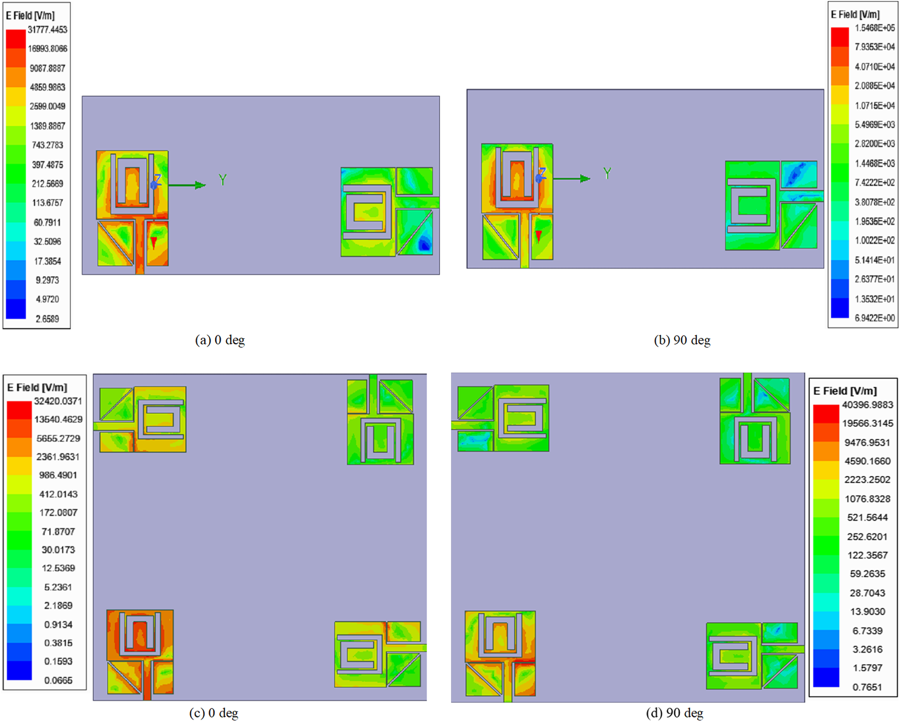
Figure 16(a–d) illustrates the electric field distribution at different phase angles (0°, 90°) for both 2 and 4P MIMO systems. It also demonstrates radiation symmetry and coupling characteristics.
Electric-field distribution of the proposed MIMO antennas at different excitation phases: (a, b) 2-port MIMO and (c, d) 4-port MIMO.

Figure 16 Long description
Four electric-field distribution heatmaps compare two-port and four-port MIMO antenna configurations at two excitation phases: 0 degrees and 90 degrees. Each heatmap displays the electric-field magnitude across the antenna plane, with the color scale on the right side of each panel labeled E Field in V m superscript -1. The first heatmap shows the two-port MIMO configuration at 0 degrees excitation phase. The color scale ranges from approximately 0.5029 at the lower end to 1993.4446 at the upper end. High field magnitude regions are concentrated near the inner driven element and surrounding ring structures. The field is more intense at specific points along the driven element edges. The second heatmap shows the two-port MIMO configuration at 90 degrees excitation phase. The color scale ranges from approximately 1.4609 times 10 superscript minus 4 at the lower end to 2.0000 at the upper end. The field distribution shifts compared to the 0 degrees case, with intensity redistributed across the antenna plane. The third heatmap shows the four-port MIMO configuration at 0 degrees excitation phase. The color scale ranges from approximately 0.0000 at the lower end to 35428.2031 at the upper end. The field magnitude is noticeably higher overall compared to the two-port configuration, with peak intensity concentrated near multiple driven elements distributed across the antenna plane. The fourth heatmap shows the four-port MIMO configuration at 90 degrees excitation phase. The color scale ranges from approximately 0.7897 at the lower end to 40396.9883 at the upper end. The peak field magnitude is the highest across all four panels. Intense regions appear near the driven elements and the distribution pattern differs from the 0 degrees case for the same four-port configuration. In all four panels, a coordinate axis marker labeled Y is visible within the antenna plane, indicating spatial orientation. The two-port configuration shows a more spatially concentrated field pattern, while the four-port configuration shows higher peak magnitudes with field activity distributed across more driven element locations. Changing the excitation phase from 0 degrees to 90 degrees visibly alters the spatial distribution of high-magnitude field regions in both configurations.
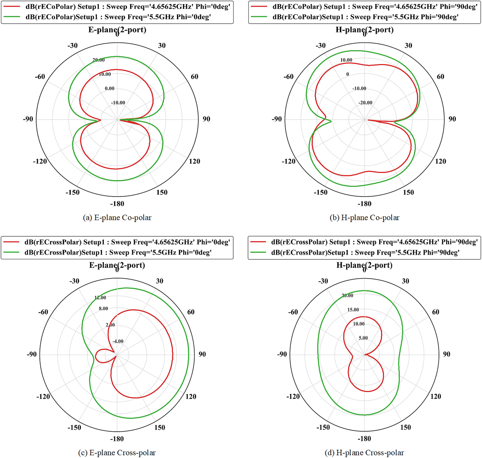
Figure 17(a–d) includes both E- and H-plane patterns at two key frequencies where the return loss is optimal. The subfigures also include co-polar vs. cross-polar patterns to identify polarization purity of the 2P MIMO design.
Simulated radiation patterns of the proposed 2P-MIMO-MPA at 4.7 GHz and 5.5 GHz showing (a, b) co-polarization and (c, d) cross-polarization characteristics.

Figure 17 Long description
The plots illustrate simulated radiation patterns of a 2P-MIMO-MPA at 4.65625 GHz and 5.5 GHz. Each plot has an angular axis labeled theta in degrees, ranging from minus 180 to 180 and a radial axis labeled magnitude in decibels. The E-plane co-polar plot shows two main lobes with peaks near minus 180 degrees and 180 degrees, with the 5.5 GHz trace having a broader lobe and higher magnitude around minus 10 decibels compared to the 4.65625 GHz trace. The H-plane co-polar plot also displays two lobes, with the 5.5 GHz trace showing a narrower shape and higher peaks. The E-plane cross-polar plot features a larger lobe at 5.5 GHz with peaks around minus 10 decibels, while the 4.65625 GHz trace shows a smaller lobe with a deep null near minus 90 degrees. The H-plane cross-polar plot has a tall narrow shape at 5.5 GHz with peaks near minus 180 degrees and 180 degrees, while the 4.65625 GHz trace forms a smaller two-lobed shape. Co-polarization refers to the alignment of the electric field with the antenna′s polarization, while cross-polarization indicates orthogonal alignment. Phi represents the azimuthal angle, with 0 degrees for E-plane and 90 degrees for H-plane. The plots highlight differences in lobe width and peak magnitudes between the two frequencies, with the 5.5 GHz traces generally showing broader lobes and higher magnitudes.
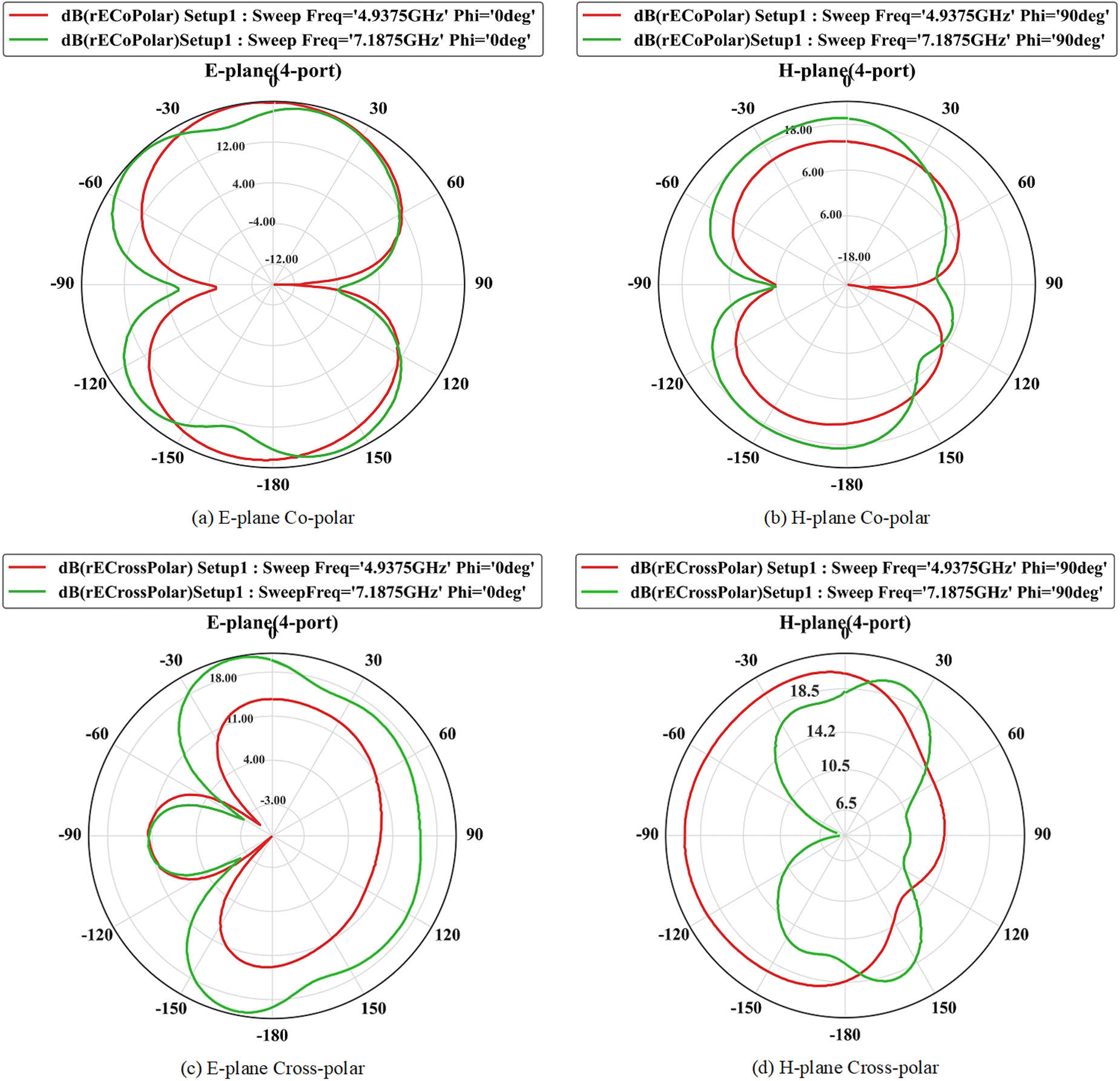
Figure 18(a–d) includes E- and H-plane plots of the proposed 4P-MIMO-MPA at 4.94 and 7.19 GHz and includes co-polar vs. cross-polar patterns, which indicate good polarization purity.
Simulated radiation patterns of the proposed 4P-MIMO-MPA at 4.94 GHz and 7.19 GHz showing (a, b) co-polarization and (c, d) cross-polarization characteristics.

Figure 18 Long description
A polar line graph labeled E-plane (plus 0 port) and the caption text (a) E-plane Co-polar. The plotted quantity in the legend is dB(rECoPolar). The angle markings are 0, 30, 60, 90, 120, 150, 180, minus 150, minus 120, minus 90, minus 60, minus 30 degrees. The radial tick labels are minus 12.00, minus 8.00, minus 4.00, 0.00. Legend entries: dB(rECoPolar) Setup1: Sweep Freq equals 4.9375GHz Phi equals 0deg; dB(rECoPolar) Setup1: Sweep Freq equals 7.1875GHz Phi equals 0deg; dB(rECoPolar) Setup1: Sweep Freq equals 7.1875GHz Phi equals 90deg. The three traces form a two-lobed shape with a narrow region near 0 degrees and a broader region around 180 degrees. The traces pass near the 0.00 ring around 0 degrees and around 180 degrees and pass closer to the minus 12.00 ring around plus or minus 90 degrees. The image B showing a polar line graph labeled H-plane (plus 0 port) and the caption text (b) H-plane Co-polar. The plotted quantity in the legend is dB(rECoPolar). The angle markings are 0, 30, 60, 90, 120, 150, 180, minus 150, minus 120, minus 90, minus 60, minus 30 degrees. The radial tick labels are minus 18.00, minus 12.00, minus 6.00, 0.00. Legend entries: dB(rECoPolar) Setup1: Sweep Freq equals 4.9375GHz Phi equals 90deg; dB(rECoPolar) Setup1: Sweep Freq equals 7.1875GHz Phi equals 90deg; dB(rECoPolar) Setup1: Sweep Freq equals 7.1875GHz Phi equals 0deg. The traces form a two-lobed shape with the outermost radius near 0 degrees and near 180 degrees and reduced radius near plus or minus 90 degrees. One trace shows a deeper inward notch on the right side between about 60 degrees and 120 degrees, reaching near the minus 18.00 ring. The image C showing a polar line graph labeled E-plane (plus 0 port) and the caption text (c) E-plane Cross-polar. The plotted quantity in the legend is dB(rECrossPolar). The angle markings are 0, 30, 60, 90, 120, 150, 180, minus 150, minus 120, minus 90, minus 60, minus 30 degrees. The radial tick labels are minus 9.00, minus 6.00, minus 3.00, 0.00. Legend entries: dB(rECrossPolar) Setup1: Sweep Freq equals 4.9375GHz Phi equals 0deg; dB(rECrossPolar) Setup1: Sweep Freq equals 7.1875GHz Phi equals 0deg; dB(rECrossPolar) Setup1: Sweep Freq equals 7.1875GHz Phi equals 90deg. The traces are asymmetric, with one side extending closer to the 0.00 ring and the opposite side pulled inward toward the minus 9.00 ring. A narrow inward feature appears near 0 degrees for one trace and a broader outward bulge appears between about 120 degrees and 180 degrees. The image D showing a polar line graph labeled H-plane (plus 0 port) and the caption text (d) H-plane Cross-polar. The plotted quantity in the legend is dB(rECrossPolar). The angle markings are 0, 30, 60, 90, 120, 150, 180, minus 150, minus 120, minus 90, minus 60, minus 30 degrees. The radial tick labels are 6.5, 10.5, 14.2, 18.5. Legend entries: dB(rECrossPolar) Setup1: Sweep Freq equals 4.9375GHz Phi equals 90deg; dB(rECrossPolar) Setup1: Sweep Freq equals 7.1875GHz Phi equals 90deg; dB(rECrossPolar) Setup1: Sweep Freq equals 7.1875GHz Phi equals 0deg. One trace forms a tall lobe near 0 degrees reaching close to the 18.5 ring, with a smaller lobe near 180 degrees. Another trace stays closer to the inner rings, with a narrow waist near plus or minus 90 degrees. Across the four graphs, the co-polar plots use radial tick labels from negative values up to 0.00 and the cross-polar plots use radial tick labels from negative values up to 0.00 in the E-plane cross-polar plot and from 6.5 to 18.5 in the H-plane cross-polar plot. Each graph overlays three traces corresponding to the legend frequency and phi entries listed for that graph.
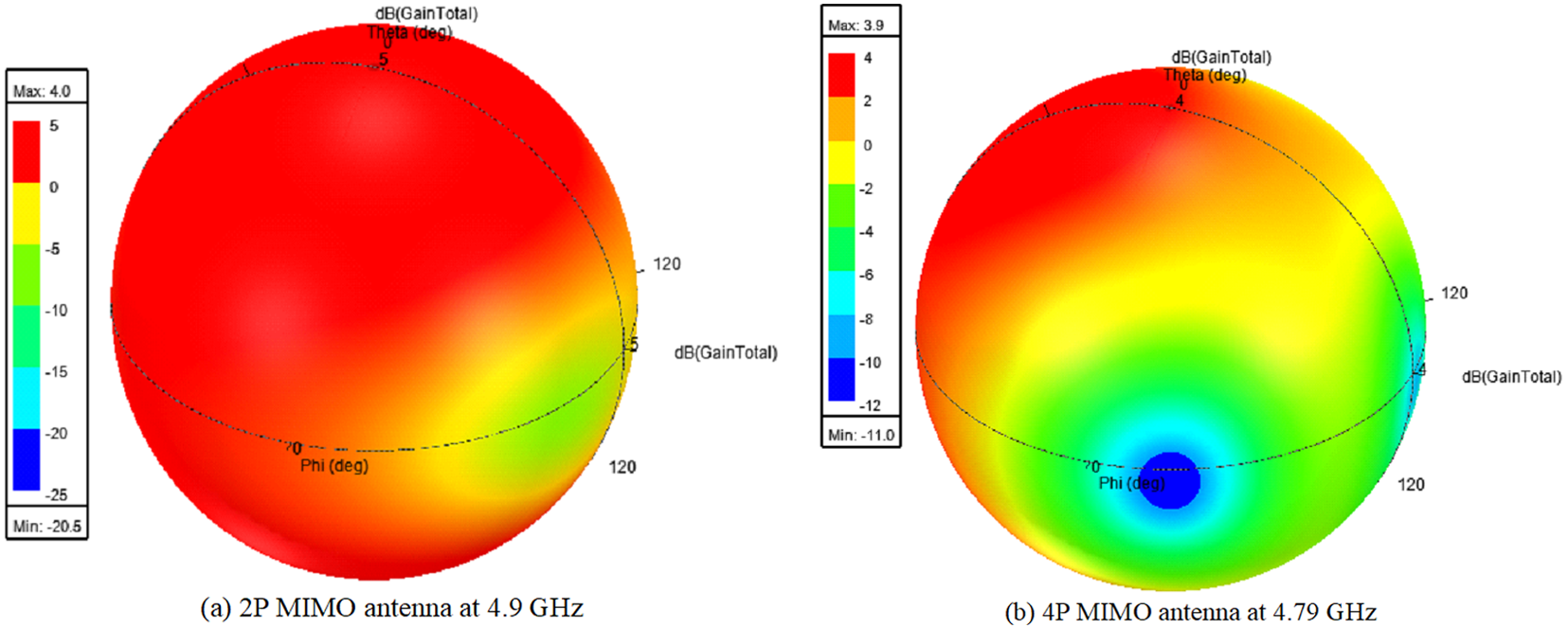
Figure 19(a, b) provides effective visual validation through the spherical plot for omnidirectional or directional performance. Accordingly, it is also seen that the 4P antenna is more directive than the 2P design.
Three-dimensional radiation patterns of the proposed (a) 2-port and (b) 4-port MIMO antennas at their respective operating frequencies.

Figure 19 Long description
Two three-dimensional spherical far-field radiation pattern plots compare the gain performance of two MIMO antenna configurations at their respective operating frequencies. The first plot is labeled 2-port MIMO antenna at 4.9 GHz. The second plot is labeled 4-port MIMO antenna at 4.79 GHz. Both plots use a spherical coordinate system with angular variables theta and phi, each expressed in degrees. The radial dimension in both plots represents gain magnitude. The color scale in both plots ranges from approximately minus 30 decibels at the lower end to 0 decibels at the upper end, with the scale labeled as decibels total. The 2-port MIMO antenna at 4.9 GHz displays a broad, near-uniform radiation pattern across the spherical surface. The gain distribution is spread widely across most of the sphere, with the maximum gain value visible on the color scale readout at the top of the plot. The 4-port MIMO antenna at 4.79 GHz displays a more concentrated radiation pattern. A dominant main lobe is visible where the gain is highest, occupying a narrower angular region compared to the 2-port case. A deep null region is also visible on the opposite side of the sphere, where gain drops toward the lower end of the scale. The maximum gain readout visible at the top of the second plot is higher than that of the first plot. The minimum gain readout is visible at the bottom of each color scale. The 2-port pattern shows energy distributed more uniformly across the sphere, while the 4-port pattern concentrates energy into a narrower main lobe with a more pronounced null region.
Experimental outcomes
Measurements were carried out using an Anritsu MS2038C Vector Network Analyzer (VNA). The system was calibrated using the standard Short–Open–Load–Through calibration technique to ensure accurate S-parameter measurements. Radiation characteristics were measured in an anechoic chamber under far-field conditions, maintaining a separation distance of at least 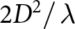 ${{2{D^2}} \mathord{\left/
{\vphantom {{2{D^2}} \lambda }} \right.
} \lambda }$. A standard horn antenna was used as the reference antenna, with proper alignment and polarization matching ensured throughout the measurements.
In order to prove the accuracy of the proposed models for the design, the measured characteristics of the prototypes of the proposed 4P MIMO-MPAs were compared to the simulations. These experiments involved VNA measurements of S-parameters along with the evaluation of radiation properties in the anechoic chamber. The prototypes under test were not only standalone MIMO antennas but also the 4P-MIMO-MPA with PFSS superstrate.
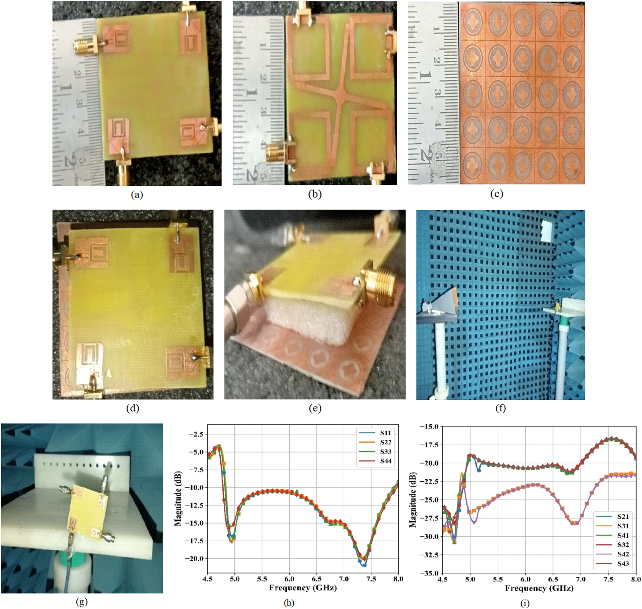
Figure 20(a–c) shows the fabricated patch, ground plane, and PFSS, respectively, whereas Fig. 20(d–g) represents the top view, isometric view, and the test chamber setup. Figure 20(h–i) shows S-parameter measurements at all ports where return loss is <−10 dB in the range of 4.69–7.885 GHz and mutual coupling is above 16 dB, which matches the simulated results. There was a slight difference between simulation and measurement results, mainly because of fabrication errors, losses from SMA connections, and the dielectric constant of the FR4 substrate. However, the measurements proved a wide impedance bandwidth, enhanced isolation, and gain obtained through the utilization of DGS and coupling structures along with the PFSS.
Fabrication and experimental validation of the proposed antenna: (a) fabricated patch, (b) ground plane, (c) FSS layer, (d, e) assembled antenna prototype, (f, g) measurement setup inside the anechoic chamber, and (h, i) measured reflection coefficients.

Discussion
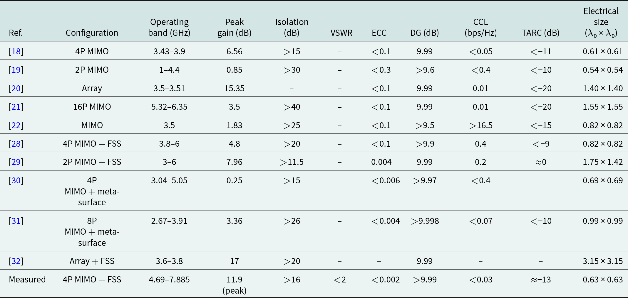
Comparative analysis brings out the advantages, disadvantages, and consequences of using DGS, network coupling, and FSS substrate for improving performance of the miniature MIMO structure. Further, comparative analysis is performed between the proposed antenna and other antennas discussed in literature. Table 3 shows the comparative assessment of different MIMO structures based on their dimensions, number of elements, bandwidth, and gain characteristics. It is observed that the performance of the proposed 2P- and 4P-MIMO-MPAs in terms of bandwidth is superior, with a range from 4.9 to 8.1 GHz for 2P and 4.69 to 7.885 GHz for 4P. It can be seen that the improved gain of 5.8 and 11.9 dB in the proposed design is much higher than <5 dB achieved by many compact antennas such as [Reference Srinubabu and Rajasekhar19, Reference Rajavel and Ghoshal22, Reference Chatterjee, Dey, Roy and Parui23].
Performance comparison of the proposed FSS-assisted MIMO antenna with existing state-of-the-art MIMO and FSS-integrated antenna designs

Table 3 Long description
Performance metrics are compared across prior antenna designs and one measured 4 port MIMO with frequency selective surface, including operating band, peak gain, isolation, VSWR, envelope correlation, diversity gain, channel capacity loss, total active reflection coefficient, and electrical size. The measured design covers roughly 4.69 to 7.885 GHz, reaches 11.9 dB peak gain, maintains isolation above 16 dB, keeps VSWR below 2, and reports very low correlation below 0.002 with diversity gain above 9.99 dB. Among earlier works, the highest listed gains are 17 dB for an array with frequency selective surface over 3.6 to 3.8 GHz and 15.35 dB for an array over 3.5 to 3.51 GHz, but both are much larger in electrical size than the measured design. Several multiport MIMO designs report stronger isolation, such as a 16 port MIMO above 40 dB and a 2 port MIMO above 30 dB, though their gains are lower than the measured design. Frequency selective surface or metasurface assisted MIMO entries generally show low correlation values, often below 0.01, with the measured design being among the lowest reported. Channel capacity loss is typically small where reported, and the measured design is below 0.03 bps per Hz, while one MIMO entry lists a much larger value above 16.5 bps per Hz, suggesting inconsistent reporting or differing definitions. Some cells are missing or use approximate or threshold values, so direct ranking across all rows should be treated cautiously.
Adding the proposed superstrate of the FSS increases the effectiveness of the design by enhancing the gain value from 5.81 to 11.91 dB. This proves that it works as an effective method of passively boosting the gain of the antenna without affecting the matching or the bandwidth. It is different from other FSS-assisted designs in that they tend to be complex, with multilayers, whereas the proposed design is single-layered but performs better than other compact designs in terms of radiation.
On the other hand, using FR4-based structures, together with the volumes of  $20 \times 50 \times 1.6\,{\text{m}}{{\text{m}}^3}$ for 2P and
 $50 \times 50 \times 1.6\,{\text{m}}{{\text{m}}^3}$ for 4P, makes the design appealing to those applications where space is limited. Nevertheless, the design does not perform well in comparison to high-gain designs like [Reference Chatterjee, Dey, Roy and Parui23] and [Reference Li, Nie, Yang, Liu, Lin and Huang32], since it does not have more than 15 dB gain, even though it is compact, has improved isolation, and can operate at frequencies below 8 GHz. Therefore, using DGS for bandwidth enhancement, coupling structures for isolation enhancement, and FSS for gain boost, the proposed design offers an excellent balance between compactness, bandwidth, and radiation, making it a good fit for sub-8 GHz wireless and mid-band 5G systems.
Conclusion
The sub-8 GHz band should still be utilized for current wireless applications because of the proper ratio of range, penetration capability, and data transmission. Nevertheless, traditional microstrip antennas suffer from the following drawbacks: narrow bandwidth, medium gain, and strong mutual coupling in the case of MIMO. The paper proposes highly efficient MIMO 2-port and 4-port microstrip antennas based on the introduction of defected ground structures, orthogonal antenna orientation, and improved coupling circuits. The designed antennas exhibit broad impedance bandwidths of 4.9–8.1 GHz (2P) and 4.69–7.885 GHz (4P) along with maximum gains of 5.8 and 11.9 dB and mutual isolation >17 dB. Additionally, the implementation of a one-dimensional FSS helps increase gain and radiation patterns while not compromising the matching performance. The measurement results are in excellent agreement with the simulated values.
The main advantage of the developed antennas compared to the previous ones is that they provide a good balance between gain, bandwidth, and size. They can be easily produced at a low cost due to the use of FR4 substrate. The antennas can be applied in sub-8 GHz 5 G/WLAN applications as well as for developing next-generation 6G technology. In the future, the proposed wideband MIMO antenna will be utilized for integrating sensing and communication functions in a single unit, that is, Integrated Sensing And Communication (ISAC) for the sixth generation of cellular networks. The wideband feature will allow radar sensing as well as range resolution, whereas the low ECC and multichannel system will enable spatial sensing and localization.

Mrs. B. Naga Prasanna is a research scholar in the Department of Electronics and Communication Engineering at Dr. M.G.R. Educational and Research Institute, Chennai. She obtained her M.Tech in Electronics and Communication Engineering with specialization in Communications and Radar and completed her B.Tech in Electronics and Instrumentation. She is a research scholar with a passionate antenna and RF systems designer with a focused interest in next-generation wireless communication technologies.

Dr. T. Kalpalatha Reddy is presently working as Professor and Additional Dean E&T at Dr. M.G.R. Educational and Research Institute, Chennai, Tamil Nadu, India. She is a reviewer for journals published by Springer and Elsevier. Presently doing her research in the area of Medical Processing Neural Networks and Biomedical Signal Processing. She is being awarded by various agencies for her contribution to the field of teaching and research. She has visited countries like China, Nepal, Vietnam, Japan, the USA, Sri Lanka, Dubai, Malaysia, and Singapore to disseminate knowledge by participating in Tech Forums. She has also published seven patents.