













Introduction
The data rate demand in satellite communication is increasing rapidly, driving the move to higher-frequency bands such as the Q-, V-, and W-bands [Reference Neff, Özat, Wörmann, Singhal, Schoch and Kallfass1–Reference Kallfass, Manoliu, Schoch, Haussmann, Koller, Tessmann, Henneberger, Steinmetz and Freese3]. To meet the high linearity requirements of higher-order modulation schemes for higher spectral efficiency, the output power of high-power amplifiers (HPAs) is typically reduced, leading to a rapidly declining power-added efficiency of the transmitter [Reference Katz, Gray and Dorval2]. Predistortion linearizers for HPAs can more than double the efficiency and add  $\approx6\,\mathrm{dB}$ of output power [Reference Katz, Gray and Dorval2, Reference Deng, Zhang, Zhou, Wang and Wang4]. The linearizer is sensitive to the signal power injected at its input, so to predistort the signal correctly, its input power must be precisely monitored [Reference Neff, Özat, Wörmann, Singhal, Schoch and Kallfass1]. For new-space applications such as low-earth orbit or very low-earth orbit satellite constellations emerging today, low-cost, highly compact, fully integrated, and versatile communication components are desired. Therefore, a highly sensitive, temperature-compensated power detector is designed in this work using a commercially available, new-space-capable IHP SG13G3Cu
 $130\,\mathrm{nm}$ silicon-germanium bipolar complementary metal-oxide-semiconductor (SiGe BiCMOS) technology for integration on chip with the linearizer. To align further with the new space approach, rather than targeting a single communication standard, the detector was intentionally designed as a highly reusable building block that can be employed across a broad range of microwave and millimeter-wave systems. In particular, its bandwidth enables operation across most major satellite communication bands, including the C-, X-, Ku-, K-, Ka-, Q-, V-, and W-bands, without requiring redesign or re-optimization of the detector core. The technology also permits monolithic integration of the presented power detector with other functional stages, such as power amplifiers [Reference Haag and Ulusoy5], transmitters [Reference Aljuhani, Kanar, Zihir and Rebeiz6, Reference Fumagalli, Colzani and Fonte7], or linearizers. A directional coupler is used to monitor the input power and implement a built-in self-test.
Integrated power detectors commonly rely on the nonlinear transfer characteristic of diodes or transistors to generate an output voltage proportional to the input power  $V_\mathrm{out}~\propto~P_\mathrm{in}$ [Reference Wei, Qayyum and Negra8]. For high-sensitivity detector designs, heterojunction bipolar transistor (HBT) or III–V technologies are typically preferred due to their inherently higher second-order transconductance, resulting in higher sensitivity than complementary metal–oxide–semiconductor (CMOS) [Reference Qayyum and Negra9–Reference Zheng, Gilreath, Jain and Heydari11].
At its simplest, a power detector uses the nonlinear transfer characteristic of a single element, such as a common-source (CS) or common-emitter (CE) transistor or a diode, achieving a high sensitivity [Reference Zheng, Gilreath, Jain and Heydari11–Reference Ildefonso, Coen, Fleetwood, Tzintzarov, Wachter, Khachatrian, McMorrow, Warner, Paki and Cressler13]. A good input-matching network (IMN) can increase sensitivity by a factor of 3 [Reference Zheng, Gilreath, Jain and Heydari11], and bandwidths above  $30\,\mathrm{GHz}$ have been reported [Reference Qayyum and Negra9, Reference Zheng, Gilreath, Jain and Heydari11, Reference Malotaux and Spirito14–Reference Cordes, Braun, Papurcu and Pohl16]. However, achieving wideband matching is difficult because the transistor or diode bias point results in a low input capacitance and, therefore, very high impedance.
Wideband detectors have been demonstrated using resistive matching [Reference Qayyum and Negra9], omitting the IMN [Reference Malotaux and Spirito14, Reference Zhou and Chia17, Reference Zhong, Han, Liu, Qi, Li and Wang18], or tolerating higher input mismatch [Reference Ozeren, Göyzu, Arslan and Kağan19, Reference Ustundag, Turkmen, Cetindogan, Kaynak and Gurbuz20]. However, a reduced input power decreases sensitivity, and the resistor’s thermal noise limits the minimum detectable power [Reference Qayyum and Negra10]. The distributed topology offers an alternative approach by absorbing the input capacitance of detector transistors into an artificial transmission line (TL) structure, resulting in relative bandwidths of up to  $200\,\mathrm{\%}$. Distributed detectors are typically realized as uniform traveling-wave detectors. CMOS implementations employ CS or common-gate (CG) transistors [Reference Wei, Qayyum and Negra8, Reference Qayyum and Negra10, Reference Wang, Liu, Ma and Han21], whereas lower-frequency implementations often use discrete diodes [Reference Qayyum and Negra22, Reference Qayyum, Wei and Negra23]. An alternative approach is a tunable narrowband detector, which optimizes the input network for a selected frequency band. Such an approach requires an additional tunable matching network and control signals, thereby significantly increasing complexity. In contrast, the proposed distributed architecture provides broadband operation without reconfiguration and can therefore be reused across multiple frequency bands without adjustments.
The detector design presented in this paper was previously published in [Reference Neff, Özat, Wörmann, Singhal, Schoch and Kallfass1]. This journal article significantly extends the previous work by providing a more detailed theoretical analysis of the nonuniform distributed detector topology, a wideband characterization of the detector and coupler up to  $110\,\mathrm{GHz}$, and the characterization of the temperature compensation. In contrast to previously reported distributed power detectors that employ uniform transistor dimensions, the proposed detector introduces a nonuniform distributed architecture in which the HBT dimensions are individually optimized for each stage. This approach enables a significant reduction in DC power consumption while maintaining the high sensitivity and ultra-wide bandwidth of the distributed detector. Furthermore, to the best of the authors’ knowledge, this work presents the first distributed power detector implemented in an HBT technology, combining the high transconductance and sensitivity of HBT devices with the wideband characteristics of a distributed architecture. Nonuniform HBT sizes are utilized to implement three identical detectors, a standalone detector, a reference for thermal compensation, and a combined combiner-detector configuration, as illustrated in Figure 4.
Nonuniform distributed power detector
Detector topology and analysis
For the analog-to-digital converters (ADCs), following the coupler-detector combination to receive a sufficiently high output voltage for a given input power, a high-voltage-sensitivity detector design is desired in this work.
For a small sinusoidal input signal with an amplitude  $V_{\mathrm{in}}=\sqrt{2P_{\mathrm{in}}Z_{\mathrm{0}}}$, the output voltage
 $V_{\mathrm{Det}}$ of a conventional CE-based power detector operating in the square-law region can be derived under the assumption of perfect matching and negligible parasitics. Assuming an input amplitude at the transistor base of
 $V_{\mathrm{B}} \approx V_{\mathrm{in}}$, the output voltage
 $V_{\mathrm{Det}}$ can be derived as [Reference Ozeren, Göyzu, Arslan and Kağan19]:
 \begin{equation}
V_{\mathrm{Det}} = V_{\mathrm{CC}}-I_\mathrm{C,0}R_{\mathrm{L}} \left( 1+\frac{V_{\mathrm{B}}^{2}}{4V_\mathrm{T}^{2}} \right),
\end{equation}
where  $V_\mathrm{T}$ is the thermal voltage,
 $I_\mathrm{C,0}=I_\mathrm{S} \:\,e^{\frac{V_{\mathrm{BE,0}}}{V_\mathrm{T}}}$ is the DC quiescent current through the transistor, and
 $R_{\mathrm{L}}$ is the load resistor.
For distributed detectors, (1) must be expanded, since they typically consist of two or more transistor stages, each of which taps the input signal voltage  $V_{\mathrm{in}}$ at different positions
 $z$ along a TL, where
 $V_{\mathrm{B}}(z=0)=V_{\mathrm{in}}$. The wave propagation along the artificial TL is described by the superposition of the forward-traveling wave
 $V^+_{\mathrm{B}}(z)$ and the backward-traveling wave
 $V^-_{\mathrm{B}}(z)$, as obtained from the solution of the telegrapher’s equation. Assuming the artificial TL is well terminated,
 $V^-_{\mathrm{B}} \lt \lt V^+_{\mathrm{B}}(z)$, yielding:
 \begin{equation}
V_{\mathrm{B}}(z)=V^-_{\mathrm{B}}(z)+V^+_{\mathrm{B}}(z) \approx V^+_{\mathrm{B}}(z)=V_\mathrm{in} e^{-\gamma z},
\end{equation}
where  $\gamma=\alpha + j\beta$ is the propagation constant with the attenuation constant
 $\alpha$ and phase constant
 $\beta$,
 $z$ is the position from the input where the
 $V_{\mathrm{B}}$ is tapped, and
 $V_\mathrm{in}$ is the amplitude of the sinusoidal input signal at the input. Substituting (2) into (1) and expanding, the equation for an n-stage distributed detector can be derived as:
 \begin{equation}
V_{\mathrm{Det}} = V_{\mathrm{CC}}-R_{\mathrm{L}} \left(\sum_{i=1}^{n} I_{\mathrm{C,0}i} \left( 1+\frac{\left(V_\mathrm{in} \cdot e^{-\gamma z_i}\right)^{2}}{4V_\mathrm{T}^{2}} \right)\right),
\end{equation}
where  $I_{\mathrm{C,0}i}$ is the DC quiescent current of stage
 $i$, and
 $z_i$ is the position from the input where the
 $i$th stage taps
 $V_\mathrm{B}$. From (3), it can now be seen that the sensitivity of the distributed detector is proportional to
 $I_{\mathrm{C,0}i}$ or
 $R_{\mathrm{L}}$ as:
 \begin{equation}
\frac{dV_{\mathrm{Det}}}{dP_{\mathrm{in}}} \propto \left(\sum_{i=1}^{n} I_{\mathrm{C,0}i}\cdot e^{-2\alpha z_i}\right)R_{\mathrm{L}},
\end{equation}
which means that increasing either  $I_{\mathrm{C,0}i}$ or
 $R_{\mathrm{L}}$ will raise the detector’s sensitivity. While
 $R_{\mathrm{L}}$ can only be modified by adjusting the supply voltage
 $V_{\mathrm{CC}}$,
 $I_{\mathrm{C,0}i}$ can be increased, for example, by using HBTs with a longer emitter length. Adding multiple emitters in parallel also raises
 $I_{\mathrm{C,0}i}$. However,
 $P_{\mathrm{in}}$ is split between the emitters, so each emitter is driven less, reducing sensitivity.
Equation (4) further indicates that the proposed distributed concept is readily scalable to a larger number of detector stages. While increasing the number of stages generally increases the overall detector sensitivity through the additional terms in the summation, the DC power consumption also increases significantly. Assuming  $R_{\mathrm{L}}$ is kept constant and equally dimensioned HBTs are employed, the quiescent current draw increases linearly, and the supply voltage
 $V_\mathrm{CC}$ must be increased to maintain the voltage drop across
 $R_{\mathrm{L}}$ for the higher quiescent current. This assumption becomes increasingly difficult to satisfy as the number of stages increases under a fixed supply voltage, since the total quiescent current rises and either a larger supply voltage or a reduction in
 $R_{\mathrm{L}}$ is required to maintain the desired collector bias. Consequently, the achievable sensitivity improvement is determined by the joint optimization of the number of stages, transistor dimensions, load resistance, and supply voltage, rather than by the number of stages alone.
Similar to uniform distributed amplifiers [Reference Campbell24], uniform distributed detectors do not evenly load their stages. Transmission-line losses and the finite base input resistance progressively attenuate the injected input wave as it propagates along the artificial TL, as described by (3). This behavior is captured by the propagation constant  $\gamma$ in (3) and introduces an exponential decay
 $e^{-\alpha z}$ of the forward-traveling wave. Consequently, this results in exponential decay of contributions from later stages to the detector’s overall sensitivity, as seen in (4) through the reduction in
 $I_{\mathrm{C,0}i}$ for larger
 $i$. Therefore, in a uniform design, the first stage will generate a larger
 $P_{\mathrm{in}}$-proportional collector current contribution than the subsequent stages.
Later stages contribute progressively less to the overall sensitivity while still consuming DC power. Consequently, a uniform stage design becomes increasingly power-inefficient as the number of stages increases. The proposed nonuniform topology addresses this by allowing the transistor dimensions, and therefore the quiescent collector current, to be optimized individually for each stage according to its expected contribution. The HBT dimensions and corresponding quiescent collector currents of the later stages can therefore be reduced compared to those of the preceding stages. This stage-dependent optimization of the emitter lengths improves the sensitivity-to-power-consumption ratio while maintaining the broadband matching characteristics of the artificial TL structure. Therefore, the proposed nonuniform topology provides greater flexibility for optimizing the sensitivity-to-power-consumption trade-off in detectors employing a larger number of stages. An equal contribution of all stages would theoretically require increasing the quiescent collector current of the later stages to compensate for the attenuation of the input wave. However, this would significantly increase the DC power consumption and diminish the benefit of the proposed nonuniform distributed topology.
Circuit implementation
In practical designs, the maximum supply voltage  $V_\mathrm{CC}$ is often fixed, which means selecting the HBT emitter lengths
 $l_\mathrm{e}$ of the detector stages is a trade-off between DC power consumption
 $P_\mathrm{DC}$,
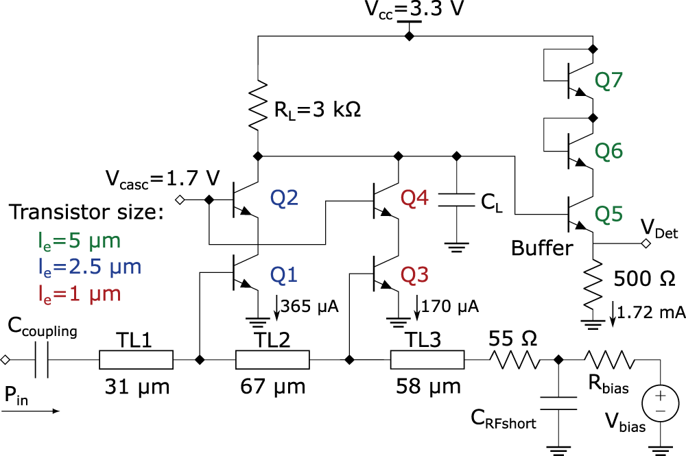
 $R_{\mathrm{L}}$, and sensitivity [Reference Neff, Özat, Wörmann, Singhal, Schoch and Kallfass1]. To illustrate this trade-off and motivate the selected two-stage implementation, a uniform and a nonuniform detector are compared using circuit simulations for a fixed
 $V_\mathrm{CC}=3.3\,\mathrm{V}$. Both detector configurations are independently optimized to achieve comparable broadband input matching over the target frequency range. For the uniform design,
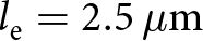 $l_{\mathrm e}=2.5\,{\mu}\mathrm m$ is selected for both stages, resulting in
 $R_{\mathrm L}=2.1\,\mathrm{k}\Omega$,
 $P_\mathrm{DC}=3.09\,\mathrm{mW}$, and a sensitivity of
 $50\,\mathrm{kV\,W^{-1}}$ at
 $45\,\mathrm{GHz}$. For the nonuniform design, the configuration shown in Figure 1 is used, reducing the second-stage emitter length to
 $l_\mathrm{e}=1$ µm. This increases
 $R_{\mathrm L}=3\,\mathrm{k}\Omega$ to maintain equal bias conditions. An approximate one-third reduction in
 $P_\mathrm{DC}$ to
 $P_\mathrm{DC}=2.16\,\mathrm{mW}$ and a sensitivity of
 $49.2\,\mathrm{kV\,W^{-1}}$ at
 $45\,\mathrm{GHz}$ is achieved. Therefore, a nonuniform design can achieve almost identical sensitivity while significantly reducing
 $P_\mathrm{DC}$ compared to a uniform design.
Schematic of the proposed nonuniform distributed detector core adapted from [Reference Neff, Özat, Wörmann, Singhal, Schoch and Kallfass1].

Figure 1 Long description
The detector circuit includes transistors labeled Q1, Q2, Q3, Q4, Q5, Q6 and Q7. Transistor sizes are indicated as l subscript e equals 5 micrometers, 2.5 micrometers and 1 micrometers. The circuit operates with a supply voltage V subscript CC of 3.3 Volts and a cascade voltage V subscript casc of 1.7 Volts. A load resistor R subscript L of 3 kiloohms is connected to the circuit. The input signal P subscript in passes through a coupling capacitor C subscript coupling and transmission lines TL1, TL2 and TL3 with lengths of 31 micrometers, 67 micrometers and 58 micrometers, respectively. The circuit includes a buffer and a detection voltage V subscript Det. A resistor of 500 Ohms is connected to the buffer, with a current of 1.72 milliamperes. The circuit also features a bias resistor R subscript bias and a bias voltage V subscript bias. Capacitors C subscript L and C subscript RFshort are present, with no ratings shown. The current through Q1 is 365 microamperes and through Q3 is 170 microamperes. Connections are made between the transistors, resistors and capacitors, forming a network for signal processing.
In a CE-HBT detector, the broadband matching can be degraded by output loading due to the limited input-output isolation [Reference Ozeren, Göyzu, Arslan and Kağan19]. As a secondary effect, the collector-base capacitance  $C_\mathrm{cb}$ varies with
 $P_{\mathrm{in}}$ because the current through
 $R_\mathrm{L}$ and the corresponding collector voltage change, introducing a weak
 $P_{\mathrm{in}}$ dependence of the transistor input impedance. Since the distributed detector relies on an artificial TL formed by the inductive TL sections and the transistor input capacitances, these effects degrade the broadband matching. A cascode configuration significantly improves the input-output isolation, thereby reducing the influence of output loading on the input impedance while maintaining a more constant collector voltage across the CE transistor, which minimizes variations in
 $C_\mathrm{cb}$ at large
 $P_{\mathrm{in}}$. Therefore, the cascode configuration shown in Figure 1 was adopted for the proposed two-cell detector to achieve simultaneous wideband small- and large-signal matching.
RF power  $P_{\mathrm{in}}$ is coupled to the input artificial TL of the detector via a large capacitance
 $C_\mathrm{coupling}=4\,\mathrm{pF}$. Since the transistor input capacitances vary with the emitter lengths along the bottom TL, the TL segment lengths are adjusted to
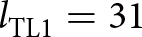 $l_\mathrm{TL1}=31$ µm,
 $l_\mathrm{TL2}=67$ µm, and
 $l_\mathrm{TL3}=58$ µm. The TLs are implemented with a width of
 $w_\mathrm{TL}=2.4$ µm, narrower than a
 $50\,{\Omega}$ TL (
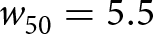 $w_\mathrm{50}=5.5$ µm), providing higher inductance per unit length and reducing the required physical length and detector area. It is further beneficial for the inductance, and therefore the impedance, of the bottom TL to be slightly larger than
 $50\,{\Omega}$, since this is shown to increase high-frequency input matching [Reference Qayyum and Negra22]. The bottom TL is therefore RF-terminated with a
 $55\,{\Omega}$ resistor, which slightly improves sensitivity while balancing input matching, followed by a capacitor
 $C_\mathrm{RFshort}=4\,\mathrm{pF}$ to ground potential.
The detector is biased with  $V_\mathrm{bias}=0.8\,\mathrm{V}$ through
 $R_{\mathrm{bias}}=1\,\mathrm{k}\Omega$, resulting in a quiescent collector current of 365 µA through Q1 and Q2 and 170 µA through Q3 and Q4. The emitter follower is biased at
 $1.72\,\mathrm{mA}$. The detector current was selected as a trade-off between sensitivity, square-law dynamic range, bandwidth, and DC power consumption. In contrast, the higher emitter-follower current is designed to provide a sufficiently low output impedance to drive the off-chip measurement setup.
Contrary to distributed amplifiers, the electrical length and impedance of the upper output TL can be ignored so long as the current-carrying capability is given, as the desired output of the detector is a DC voltage and the remaining high-frequency components are filtered by the output low-pass filter consisting of  $R_{\mathrm{L}}$ and
 $C_\mathrm{L}=3\,\mathrm{pF}$.
In the breakout chip, which is used for evaluation of the designed circuits, an emitter follower buffer is employed to isolate the detector core from the output node and the external measurement environment. While power detectors are typically loaded with a high-ohmic input, the buffer is included in this implementation to minimize the influence of parasitic capacitances and loading effects introduced by the measurement setup, including the connection to the vector network analyzer (VNA)’s external ADC via a long coaxial cable. The low output impedance of the emitter follower enables fast charging and discharging of the cable capacitance, ensuring that the measured detector voltage accurately follows the detector response during frequency sweeps. In a fully integrated implementation with a nearby ADC input, this buffer stage may be omitted to reduce power consumption. Two diode-connected HBTs reduce  $V_\mathrm{CC}$ to supply the buffer and protect the buffer transistor by reducing the maximum base-collector voltage. This is required because, depending on the input power level, the buffer base voltage varies between 0.8 and
 $2.8\,\mathrm{V}$, which can otherwise result in a base-collector voltage exceeding the minimum specified breakdown voltage of the employed HBT technology.
Coupler
Figure 2 shows the coupler that directs a small fraction of the input power to the on-chip power detector. Conventional monolithic microwave integrated circuit (MMIC) couplers are typically implemented as edge-side-coupled TLs on the same metal layer. In this work, a broadside-coupled design is chosen to reduce the occupied area, as illustrated by the cross-sectional views in Figure 2(a) and (b). For the two coupler topologies to achieve equal coupling factors of  $\approx 15\,\mathrm{dB}$ between the two lines, an edge-side coupler would need a spacing of 9.1 µm between two microstriplines on the top thick copper layer. The choice of TL layers sets the baseline coupling in the broadside design. Their width and overlap can be adjusted to fine-tune the coupling factor at the cost of impedance matching. The top line on the thick copper layer is chosen as the through line to the linearizer because it has the lowest loss due to its thickness. The bottom layer is realized on the fourth thin metal layer. The process specifications set the broadside coupler spacing to 4.46 µm. The broadside coupler achieves lower coupling at a closer distance because the bottom TL width (2 µm) is smaller than the thickness of the thick copper layer (3.2 µm).
Overview of the proposed broadside directional coupler showing (a) the cut section view of an edgeside coupler, and (b) the cut section view, (c) the top view, and (d) a photograph of the fabricated breakout chip of the broadside coupler.

Figure 2 Long description
Four parts illustrate a broadside directional coupler. The first part, labeled a, shows the edgeside cut section with two thick copper 2 layers separated by 9.1 micrometers and a metal 3 layer below. The second part, labeled b, depicts the broadside cut section with a spacing of 4.46 micrometers between two metal layers, with a 2 micrometers width for the bottom layer. The third part, labeled c, presents the top view of the coupler with a zigzag pattern, marked with points P1, P2, P3 and P4 and dimensions of 154.8 micrometers by 192.2 micrometers. The fourth part, labeled d, is a photograph of the fabricated breakout chip, showing a layout with labeled points P1, P2, P3 and P4 and dimensions of 274 micrometers by 312 micrometers. The materials are color-coded: thick copper 2 in yellow, metal 4 in orange, metal 3 in red and metal 2 in gray.
The detector is designed for a  $50\,{\Omega}$ environment, using a 5.5 µm-wide microstripline with the third thin metal layer as the ground plane. The broadside coupler uses the second thin metal layer as the ground because the bottom TL is too close to the third thin metal layer. The top TL must be wider at 8 µm to achieve
 $50\,{\Omega}$ matching. Per TL section, this results in an area saving of about
 $40\,\mathrm{\%}$ for the broadside design over the edgeside design, at the cost of one less layer available for routing underneath the coupler. Figure 2(c) shows the meandering of the TLs used to compact the coupler footprint, with dimensions of 155 µm
 $\times$ 192 µm.
Measurement
Coupler
The coupler was implemented once together with the detectors, Figure 4(b), and a second time as a standalone breakout chip, Figure 2(c), to confirm its performance. Its physical dimensions are largely dominated by the two RF pads at the input port P1 and at the coupled port P3. The through P2 and isolation port P4 are terminated with  $50\,{\Omega}$ resistors each to reduce area consumption by omitting two RF pads. The S-parameter measurement of the coupler was performed with a VNA, using frequency extenders and 1-mm coaxial probes at each port, to continuously measure from
 $10\,\mathrm{MHz}$ to
 $110\,\mathrm{GHz}$. Calibration was performed to the on-chip pad reference level.
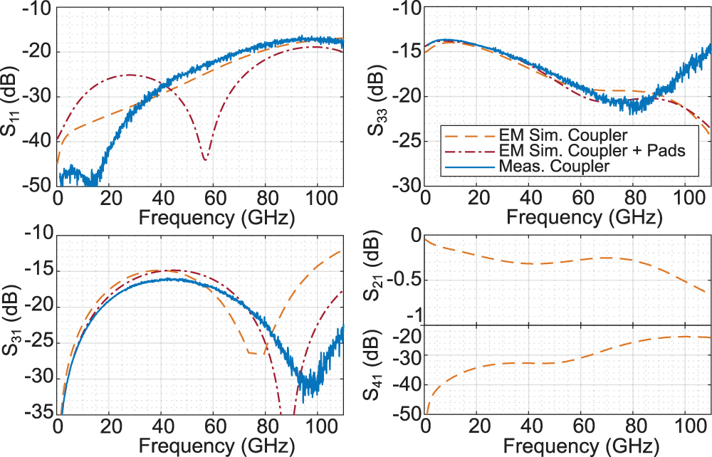
The comparison between the electromagnetic (EM) simulation performed in Cadence EMX and the measurement results is shown in Figure 3. Since the coupler is symmetrical,  $S_{11}$ and
 $S_{22}$, and
 $S_{33}$ and
 $S_{44}$ should be identical. This means that, with the implemented setup, only the isolation
 $S_{41}$ and the through
 $S_{21}$ cannot be measured for a full characterization of the coupler. The simulation results are shown in Figure 3. While
 $S_{33}$ shows excellent agreement with both EM simulations up to
 $80\,\mathrm{GHz}$,
 $S_{11}$ exhibits deviations at low frequencies
 $ \lt 30\,\mathrm{GHz}$. This behavior is attributed to the higher sensitivity of port P1 to the pad and probe parasitics, as it directly probes the frequency-dependent impedance transformation of the coupled-line structure. With the through P2 and isolated P4 ports terminated in
 $50\,{\Omega}$, the coupled port P3 exhibits an inherently broadband impedance match and is less sensitive to pad parasitics, since port P1 is isolated when injecting from P3.
Measured and simulated coupler S-parameters.

Figure 3 Long description
A four part figure with four line graphs. The image A showing a line graph with the vertical axis labeled, S subscript 11, open parenthesis decibel close parenthesis, ranging from minus 50 to minus 10. The horizontal axis is labeled, Frequency open parenthesis gigahertz close parenthesis, ranging from 0 to 110. Three curves are shown: a dashed curve labeled, EM Sim. Coupler, a dash dot curve labeled, EM Sim. Coupler plus Pads and a solid curve labeled, Meas. Coupler. The solid curve starts near minus 50 at 0, rises to about minus 47 near 10, then rises to about minus 30 near 30, about minus 25 near 40, about minus 22 near 60 and about minus 18 near 100 to 110. The dashed curve rises from about minus 40 near 0 to about minus 30 near 40, then to about minus 20 near 80 to 110. The dash dot curve rises from about minus 40 near 0 to about minus 25 near 30, then drops to about minus 45 near 55, then rises to about minus 20 near 90 to 110. The image B showing a line graph with the vertical axis labeled, S subscript 33, open parenthesis decibel close parenthesis, ranging from minus 30 to minus 10. The horizontal axis is labeled, Frequency open parenthesis gigahertz close parenthesis, ranging from 0 to 110. A legend inside the plot lists three curves: dashed, EM Sim. Coupler; dash dot, EM Sim. Coupler plus Pads; solid, Meas. Coupler. The solid curve is near minus 15 around 0 to 20, decreases to about minus 18 near 50, reaches about minus 21 near 70 to 80, then rises to about minus 15 near 110. The dashed curve is near minus 15 around 0 to 20, decreases to about minus 20 near 70, stays near minus 20 around 70 to 90, then decreases to about minus 24 near 110. The dash dot curve follows a similar path, near minus 15 around 0 to 20, decreasing to about minus 21 near 70 to 80, then decreasing further to about minus 25 near 110. The image C showing a line graph with the vertical axis labeled, S subscript 31, open parenthesis decibel close parenthesis, ranging from minus 35 to minus 10. The horizontal axis is labeled, Frequency open parenthesis gigahertz close parenthesis, ranging from 0 to 110. Three curves are shown with the same labels as the legend in image B. The solid curve rises from about minus 35 at 0 to about minus 20 near 10, reaches about minus 16 near 40 to 50, then decreases to about minus 20 near 70, reaches about minus 30 near 95 to 100 and ends near minus 24 to minus 25 near 110. The dashed curve rises from about minus 35 at 0 to about minus 15 near 40 to 50, then decreases to about minus 27 near 70, then rises to about minus 12 near 110. The dash dot curve rises from about minus 35 at 0 to about minus 15 near 40 to 50, then decreases to below minus 35 near 85 to 90, then rises to about minus 18 near 110. The image D showing a line graph with two stacked vertical scales on the left. The upper vertical scale is labeled, S subscript 21, open parenthesis decibel close parenthesis, ranging from 0 to minus 1. The lower vertical scale is labeled, S subscript 41, open parenthesis decibel close parenthesis, ranging from minus 50 to minus 20. The horizontal axis is labeled, Frequency open parenthesis gigahertz close parenthesis, ranging from 0 to 110. Two dashed curves are shown. The upper dashed curve starts near 0 at 0, is near minus 0.3 around 40 to 60 and is near minus 0.6 near 110. The lower dashed curve starts near minus 50 at 0, rises to about minus 33 near 20 to 40 and rises to about minus 22 near 100 to 110.
(a) Block diagram of the proposed circuit and (b) photograph of the fabricated chip adapted from [Reference Neff, Özat, Wörmann, Singhal, Schoch and Kallfass1].

Figure 4 Long description
A block diagram with inputs on the left and voltage outputs on the right. At the upper left, an input arrow labeled In subscript Det points right into a node labeled P subscript in, then into a block labeled Detector that contains a diode symbol. The Detector block output goes right to a node labeled V subscript Det, then to a ground symbol. A vertical line labeled V subscript out runs downward near the right side of the diagram, with arrows pointing to the right at two points: one arrow labeled V subscript Det near the top and one arrow labeled V subscript RDet below. In the middle, a block labeled Reference contains a diode symbol. The left side of the Reference block is connected to a ground symbol. The right side of the Reference block connects to the V subscript out vertical line at the level of the arrow labeled V subscript RDet. The V subscript RDet arrow points right to a ground symbol. At the lower left, a coupler section is labeled Coupler. A left input node is labeled P subscript in, with an upward arrow labeled In subscript C. From this P subscript in node, a line goes right into the Coupler block. Inside the Coupler block, a curved branch is labeled minus 15 decibel and connects upward to a vertical resistor labeled 50 ohm that ends at a ground symbol. The main coupler line continues right and is labeled approximately P subscript in. At the right end of this line, a vertical resistor labeled 50 ohm connects down to a ground symbol. From the main coupler line, a branch goes up into a second block labeled Detector that contains a diode symbol. The output of this lower Detector block goes right to an arrow labeled V subscript coup, then to a ground symbol. To the right of the coupler output area, a dashed rectangle is labeled Linearizer, Not included. The image B showing a rectangular chip photograph with dimension arrows labeled 600 micrometers across the top and 1130 micrometers along the right side. Near the top center of the chip, text reads MNLNDPDL2023. A dashed rectangular region near the upper left of the chip area is labeled 194 micrometers across and 170 micrometers vertically. Along the right edge of the chip are stacked pad labels, from top to bottom: V subscript Det, GND, V subscript cc, V subscript casc, GND, V subscript RDet, V subscript bias, GND, V subscript Coup. On the left side of the chip, a label reads In subscript Det near a pad area. Near the bottom, a label reads In subscript C near a pad area.
The measured coupling  $S_{31}$ is
 $1.15\,\mathrm{dB}$ lower than simulated, resulting in a maximum coupling of
 $S_{31}=-16.05\,\mathrm{dB}$. At the same time, the measured 3-dB bandwidth increases by
 $3\,\mathrm{GHz}$ to
 $48\,\mathrm{GHz}$, extending from 20 to
 $68\,\mathrm{GHz}$. This behavior is likely caused by substrate losses, even-/odd-mode imbalance due to fabrication tolerances, and termination parasitics, which flatten the coupling response while reducing its peak value. The center frequency of the coupling structure was shifted by
 $5\,\mathrm{GHz}$ to
 $45\,\mathrm{GHz}$ in the EM simulation and the fabricated design, compared to the simulation without RF pads, due to additional TL length that was added to facilitate transitions to other layers for termination and for connecting the coupler to the RF pads. The EM simulation shows a maximum
 $S_{41}$ of
 $-24\,\mathrm{dB}$ at frequencies above
 $90\,\mathrm{GHz}$ and a maximum loss
 $\left|S_{21}\right|= 0.7\,\mathrm{dB}$ at
 $110\,\mathrm{GHz}$ with around
 $0.4\,\mathrm{dB}$ loss at the coupling maximum of
 $45\,\mathrm{GHz}$.
Detector
To evaluate the detector and the combined performance of the coupler and the detector, the breakout chip shown in Figure 4 is manufactured. Three identical detector cells are placed in close proximity on the chip. The upper detector shown in Figure 4 in red is used to evaluate the performance of the standalone detector. By adding an identical reference detector, highlighted in Figure 4 in green, with a grounded input, the DC offset-free detector output voltage is calculated as  $V_{\mathrm{out}}=V_{\mathrm{Det}}-V_{\mathrm{RDet}}$. The third detector is placed in combination with the coupler at its input to characterize the two circuits as they would be employed in a system, for example, a linearizer. The unused through connection of the coupler is terminated by a
 $50\,{\Omega}$ resistor. Like the standalone detector, the DC offset-free output voltage
 $V_{\mathrm{out}}$ can be calculated by referencing the detector’s output voltage to the idle reference detector in the center.
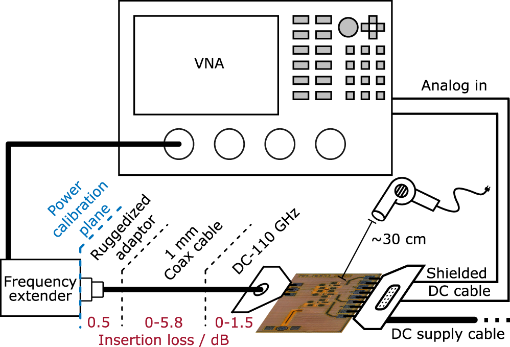
The measurement setup for the detector chip is shown in Figure 5 and differs from the S-parameter setup used to measure the coupler breakout, as only one RF port is used for the power detector’s RF input. The bias and output voltages are supplied to and from the chip via a DC probe. The two DC voltages  $V_{\mathrm{Det}}$ and
 $V_{\mathrm{RDet}}$, or
 $V_{\mathrm{Coup}}$ and
 $V_{\mathrm{RDet}}$ for the two fabricated signal paths, are fed to the internal analog inputs of the VNA. They are sampled by two
 $\pm 10\,\mathrm{V}$ 14 bit ADCs with a typical resolution of
 $1.22\,\mathrm{mV}$. For the RF probe, a thru–reflect–line (TRL) calibration using a second RF probe and a commercial calibration substrate was performed, moving the reference plane for the S-parameter measurement to the probe tips. The reported measurements, therefore, include the RF pad parasitics. Power calibration could only be performed directly at the output of the frequency extenders. Each measurement is corrected by de-embedding the frequency-dependent insertion loss of the ruggedized coaxial adapter, the
 $50\,\mathrm{cm}$ 1-mm coaxial cable, and the 1-mm coaxial RF probes. The measurement setup is identical to [Reference Neff, Özat, Wörmann, Singhal, Schoch and Kallfass1], except that a 1.85-mm coaxial cable, probe, and power calibration up to
 $67\,\mathrm{GHz}$ were used in [Reference Neff, Özat, Wörmann, Singhal, Schoch and Kallfass1].
Measurement setup used to measure the transfer characteristic and thermal compensation of the detector.

Figure 5 Long description
The measurement setup features a Vector Network Analyzer (VNA) at the top center, connected to an analog input on the right. Below the VNA, a frequency extender is positioned on the left, linked to the VNA via a ruggedized adaptor and a one millimeter coaxial cable. The cable is labeled with insertion loss values ranging from zero point five to five point eight decibels. The coaxial cable extends to a printed circuit board at the bottom right, which is connected to a shielded DC cable approximately thirty centimeters long. A DC supply cable is also shown extending from the circuit board. The power calibration plane is marked near the frequency extender, indicating the calibration setup. The entire configuration is designed to measure specific characteristics using the VNA and associated components.
During the S-parameter measurements, a constant uncorrected  $P_\mathrm{in}=-15\,\mathrm{dBm}$ is applied to the detector, while
 $P_\mathrm{in}=-5\,\mathrm{dBm}$ is used for the coupler and detector combination. These values represent the power levels at the output of the frequency extender. S-parameters are subsequently corrected through calibration. Therefore, the frequency-dependent variation of
 $P_\mathrm{in}$ is only relevant to the drive level of the detector. The artificial TL structure mainly determines detector matching, and the base-collector capacitance is compensated for changes in
 $P_\mathrm{in}$ through the cascode implementation in each detector cell. As a result, power-dependent S-parameter changes are negligible. The comparison of the measured and simulated
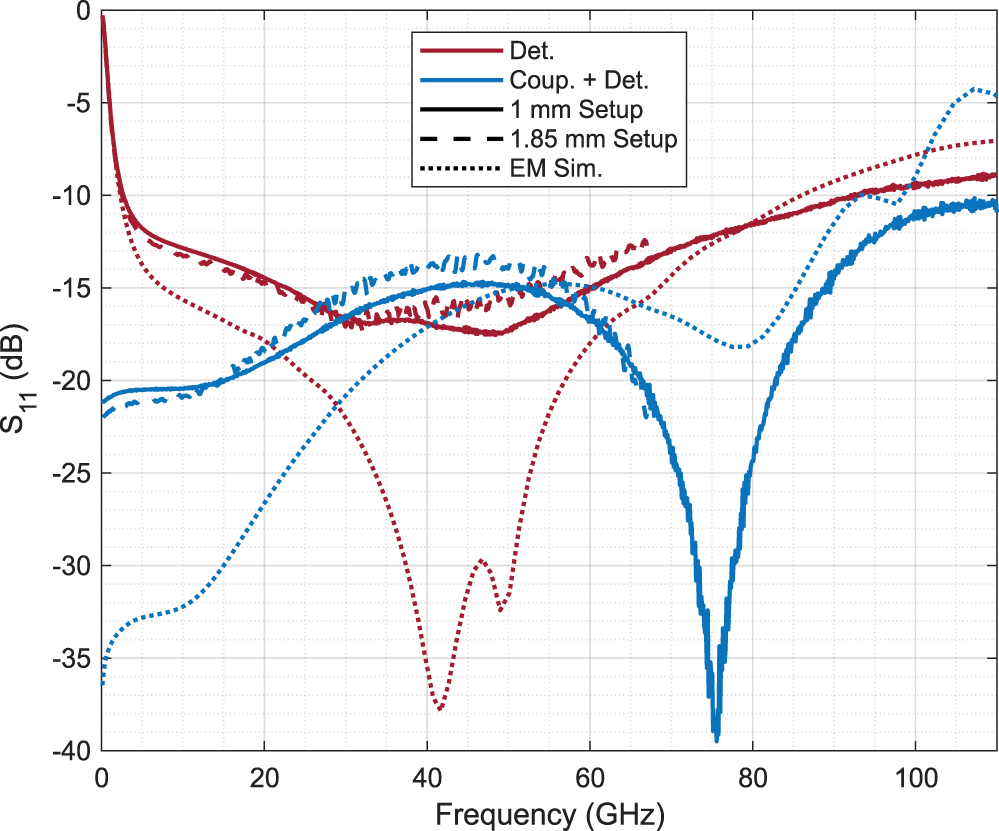
 $S_{11}$ is shown in Figure 6 and includes the
 $S_{11}$ measurement from [Reference Neff, Özat, Wörmann, Singhal, Schoch and Kallfass1] with the 1.85-mm coaxial setup. In [Reference Neff, Özat, Wörmann, Singhal, Schoch and Kallfass1], the
 $S_{11}$ measurement of the standalone detector shows a strong frequency shift of the minimum by more than
 $5\,\mathrm{GHz}$ and only a single minimum, which reduces the matching bandwidth. New measurements, shown in Figure 6, of the standalone detector with the 1-mm coaxial setup show improved performance and better agreement with simulations, due to better calibration and improved contact between the on-wafer probes and the wafer surface. These new measurements agree well with the two-minima behavior observed in
 $S_{11}$ in EM simulation and match the
 $S_{11}$ measurement performed using the 1-mm coaxial setup. The measured standalone detector shows a below
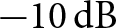
 $-10\,\mathrm{dB}$
 $S_{11}$ bandwidth of
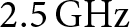
 $90\,\mathrm{GHz}$ from 2.5 to
 $92.5\,\mathrm{GHz}$, resulting in a relative bandwidth of
 $190\,\mathrm{\%}$. The measured
 $S_{11}$ in Figure 6 of the coupler and detector combination is mainly dominated by the coupler’s
 $S_{11}$. The measurement using the 1-mm coaxial setup shows good agreement with that of the 1.85-mm coaxial setup in [Reference Neff, Özat, Wörmann, Singhal, Schoch and Kallfass1]. The differences between the simulated and measured
 $S_{11}$ are likely caused by the metal filler structures above the coupler, which were omitted in the EM simulation. These structures are required to satisfy the local metal-density rules of the SiGe process.
Measured and simulated  $S_{11}$ of the standalone detector and the coupler + detector combination with the 1-mm setup compared to the measured results from [Reference Neff, Özat, Wörmann, Singhal, Schoch and Kallfass1] with the 1.85-mm setup.

Figure 6 Long description
The legend lists, Det., Coup. plus Det., 1 millimeter Setup, 1.85 millimeter Setup and EM Sim. The horizontal axis is labeled, Frequency in gigahertz, ranging from 0 to 110 with labeled ticks at 0, 20, 40, 60, 80 and 100. The vertical axis is labeled, S subscript 11 in decibel, ranging from 0 to minus 40 with labeled ticks at 0, minus 5, minus 10, minus 15, minus 20, minus 25, minus 30, minus 35 and minus 40. Detector curves: One detector curve starts near 0 decibel at 0 gigahertz, drops to about minus 12 decibel by about 5 gigahertz, then stays between about minus 12 and minus 18 decibel from about 5 to 60 gigahertz, with a shallow minimum around the mid band near about minus 17 to minus 18 decibel. From about 60 to 110 gigahertz it rises gradually, reaching about minus 9 to minus 10 decibel near 100 to 110 gigahertz. A detector simulation curve shows two deep minima in the mid band, reaching about minus 38 decibel near about 42 gigahertz and about minus 33 decibel near about 48 gigahertz, then rising toward about minus 7 to minus 8 decibel by about 110 gigahertz. Coupler plus detector curves: A coupler plus detector curve begins near about minus 21 to minus 22 decibel at 0 gigahertz, rises to about minus 15 decibel by about 40 to 50 gigahertz, then drops to a deep minimum near about minus 39 to minus 40 decibel around about 75 gigahertz. After this minimum it rises to about minus 12 decibel near about 95 gigahertz and about minus 10 to minus 11 decibel near about 110 gigahertz. A coupler plus detector simulation curve rises from about minus 36 decibel at 0 gigahertz to about minus 15 decibel near about 55 to 60 gigahertz, dips to about minus 18 decibel near about 75 gigahertz, then rises and reaches about minus 5 decibel near about 105 to 110 gigahertz.
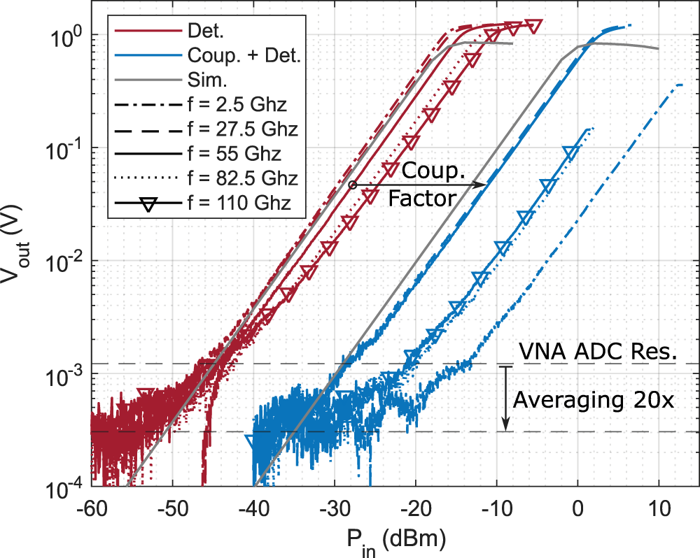
For the measurement of the transfer characteristic  $V_{\mathrm{out}}$ vs.
 $P_{\mathrm{in}}$, the frequency of the input signal in Figure 7 is kept constant, while sweeping
 $P_{\mathrm{in}}$ starting from
 $-60\,\mathrm{dBm}$ and measuring the DC output voltages of the detector at each step. The upper limit of the sweep was adjusted based on the detector’s sensitivity at the examined frequency. The measured
 $V_{\mathrm{out}}$ vs.
 $P_{\mathrm{in}}$ data have been corrected for the frequency-dependent insertion loss of the measurement setup.
 $P_{\mathrm{in}}$ is the power injected directly from the probe tip.
Measured and simulated  $V_{\mathrm{out}}$ vs.
 $P_{\mathrm{in}}$ of the standalone detector and the coupler + detector combination.

Figure 7 Long description
The y-axis label is, V out, with unit, V. The y-axis uses logarithmic tick labels, 10 superscript 0, 10 superscript minus 1, 10 superscript minus 2, 10 superscript minus 3 and 10 superscript minus 4. The x-axis label is, P in, with unit, decibel milliwatt. The x-axis tick labels are minus 60, minus 50, minus 40, minus 30, minus 20, minus 10, 0 and 10. A legend box lists three series labels, Det., Coup. plus Det. and Sim. It also lists five frequency entries: f equals 2.5 Ghz, f equals 27.5 Ghz, f equals 55 Ghz, f equals 82.5 Ghz and f equals 110 Ghz. Two main groups of rising curves are shown. One group is positioned on the left side of the plot and spans roughly from P in near minus 60 to about minus 10, with V out rising from around 10 superscript minus 4 up to around 10 superscript 0. A second group is positioned to the right and spans roughly from P in near minus 40 to about plus 10, with V out rising from around 10 superscript minus 4 up to around 10 superscript 0. An annotation near the middle reads, Coup. Factor, with a horizontal arrow pointing from the left group toward the right group. Near the lower right, text reads, VNA ADC Res. Below it, text reads, Averaging 20x. A vertical double headed arrow is drawn beside this text, spanning between two horizontal dashed reference lines in the lower portion of the plot.
The lower limit of the  $V_{\mathrm{out}}$ measurement from [Reference Neff, Özat, Wörmann, Singhal, Schoch and Kallfass1] was limited by the ADC resolution of the VNA’s analog inputs. For this measurement setup, the DC measurement was averaged 20 times using successive capture averaging in the VNA. This reduces the measurement noise and improves the effective number of bits of the VNA ADC from 14 bits to 16.16 bits, reducing the effective voltage resolution to
 $\approx 276$ µV [Reference Zheng, Zhao, Zhou, Wang and Jiang25], as shown in Figure 7. The
 $V_{\mathrm{out}}$ vs.
 $P_{\mathrm{in}}$ characteristic was measured in
 $2.5\,\mathrm{GHz}$ steps from 2.5 to
 $110\,\mathrm{GHz}$, with five of the measured curves at equally spaced frequencies shown in Figure 7 for the two circuit variants fabricated. At
 $55\,\mathrm{GHz}$, the transfer characteristic of the standalone detector and the combined coupler and detector are separated by
 $\approx 17\,\mathrm{dB}$, which corresponds directly with the simulated and measured performance of the standalone coupler, shown in Figure 3. EM simulation and measurement agree well, showing a slightly higher loss but an
 $\approx 2\,\mathrm{dB}$ increase in linearity at high
 $P_{\mathrm{in}}$ levels. The coupler-detector combination shows early compression in the
 $V_{\mathrm{out}}$ curves at 2.5, 82.5, and
 $110\,\mathrm{GHz}$. This behavior is caused by the limited output power of the frequency extenders, which is typically restricted to
 $12\,\mathrm{dBm}$ at
 $2.5\,\mathrm{GHz}$ and
 $2\,\mathrm{dBm}$ above
 $64\,\mathrm{GHz}$. The detector measurement remains noise-limited near the ADC resolution, even after averaging.
The sensitivity of the measured  $V_{\mathrm{out}}$ vs.
 $P_{\mathrm{in}}$ characteristics is calculated in the square-law region around the offset-corrected
 $P_{\mathrm{in}}=-20\,\mathrm{dBm}$ for the standalone detector and around
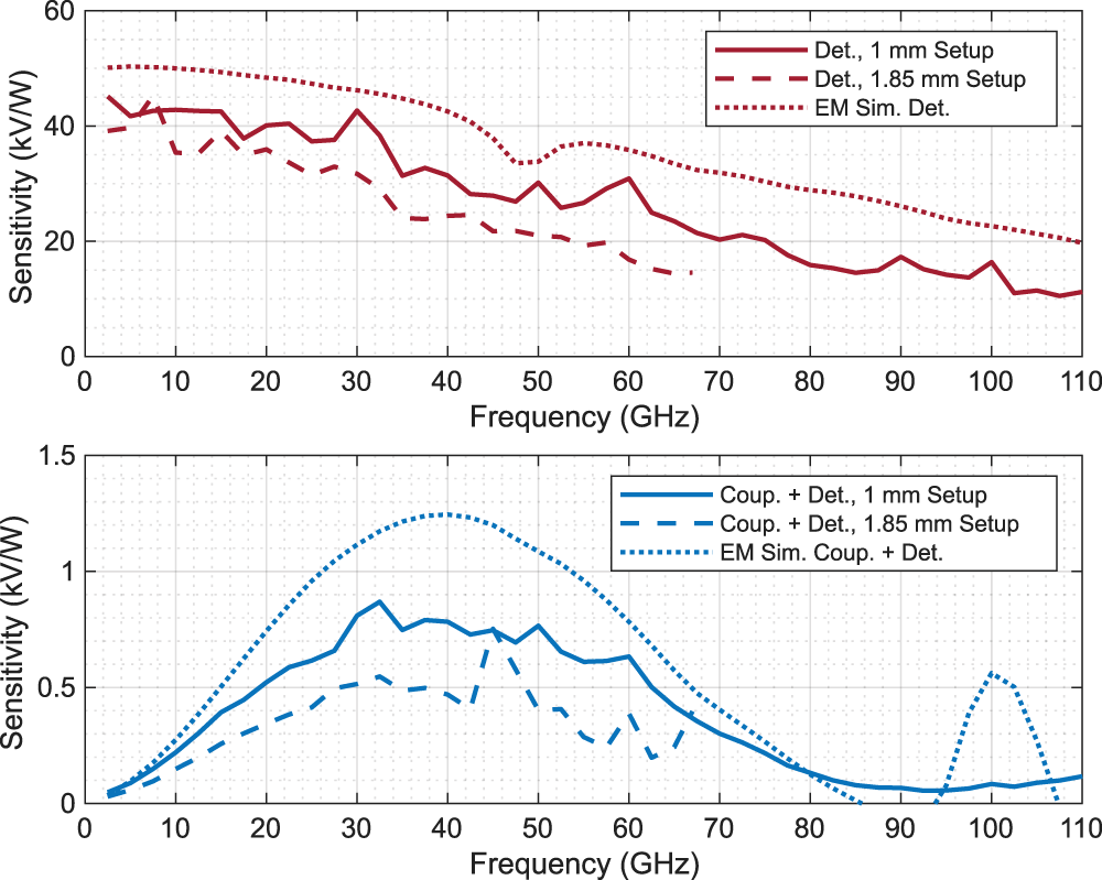
 $P_{\mathrm{in}}=-3\,\mathrm{dBm}$ for the combined circuit. As seen in Figure 8, a higher sensitivity was measured with the
 $1\,\mathrm{mm}$ coaxial setup than in [Reference Neff, Özat, Wörmann, Singhal, Schoch and Kallfass1] due to improved frequency-dependent compensation of the external losses in the measurement setup, improved contact, and calibration. Therefore, a sensitivity of
 $45.12\,\mathrm{kV\,W^{-1}}$ at
 $2.5\,\mathrm{GHz}$ to
 $10.51\,\mathrm{kV\,W^{-1}}$ at
 $107.5\,\mathrm{GHz}$ is measured for the standalone detector, showing a clear downward trend for higher frequencies. The near-constant simulated offset of approximately
 $9\,\mathrm{kV\,W^{-1}}$ over the entire measured bandwidth suggests a frequency-independent scaling error. This deviation is likely caused by unaccounted losses in the interconnections, probes, or DC bias network, as well as slight differences between the simulated and measured bias conditions of the detector cells. For the combined coupler and detector circuit, this trend continues, with the coupler’s coupling behavior clearly dictating the circuit’s sensitivity vs. frequency behavior. The simulation trend is followed more closely by the 1-mm setup than by the measurement in [Reference Neff, Özat, Wörmann, Singhal, Schoch and Kallfass1], with fewer extreme outliers due to the aforementioned frequency-dependent loss compensation in the measurement periphery. Peak sensitivity is achieved around the maximum of the coupling factor around
 $32.5\,\mathrm{GHz}$ with
 $869\,\mathrm{V\,W^{-1}}$ and 49 and
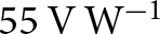 $55\,\mathrm{V\,W^{-1}}$ at 2.5 and
 $92.5\,\mathrm{GHz}$, respectively.
Measured and simulated sensitivity vs. frequency of the standalone detector and the coupler + detector combination with the 1-mm setup compared to the measured results from [Reference Neff, Özat, Wörmann, Singhal, Schoch and Kallfass1] with the 1.85-mm setup.

Figure 8 Long description
The line graph A has three curves and a legend listing, Det., 1 mm Setup, Det., 1.85 mm Setup and EM Sim. Det. The x-axis label is Frequency, in gigahertz, with tick labels from 0 to 110 in steps of 10. The y-axis label is Sensitivity, in kilovolt per watt, with tick labels at 0, 20, 40 and 60. The solid curve starts near 45 at about 5 gigahertz, stays near 40 to 45 through about 30 gigahertz, then declines with fluctuations to about 30 near 60 gigahertz, about 20 near 70 gigahertz, about 15 near 85 gigahertz and about 10 near 110 gigahertz. The dashed curve starts near 40 at about 5 gigahertz, declines to about 35 near 20 gigahertz, about 30 near 30 gigahertz, about 25 near 40 gigahertz and about 15 near 65 gigahertz where the curve ends. The dotted curve starts near 50 at about 5 gigahertz, declines to about 45 near 30 gigahertz, about 40 near 40 gigahertz, dips to about 33 near 50 gigahertz, rises to about 37 near 55 gigahertz, then declines to about 30 near 75 gigahertz and about 20 near 110 gigahertz. The line graph B has three curves and a legend listing, Coup. plus Det., 1 mm Setup, Coup. plus Det., 1.85 mm Setup and EM Sim. Coup. plus Det. The x-axis label is Frequency, in gigahertz, with tick labels from 0 to 110 in steps of 10. The y-axis label is Sensitivity, in kilovolt per watt, with tick labels at 0, 0.5, 1.0 and 1.5. The solid curve starts near 0 at 0 gigahertz, rises to about 0.4 near 15 gigahertz, about 0.6 near 25 gigahertz, peaks near 0.85 around 32 gigahertz, then declines to about 0.7 near 50 gigahertz, about 0.5 near 65 gigahertz, about 0.2 near 75 gigahertz and near 0.05 around 90 to 100 gigahertz, ending near 0.1 at 110 gigahertz. The dashed curve starts near 0 at 0 gigahertz, rises to about 0.3 near 20 gigahertz, about 0.5 near 30 gigahertz, reaches about 0.7 near 45 gigahertz, then drops to about 0.3 near 55 gigahertz, fluctuates between about 0.2 and 0.4 from about 55 to 70 gigahertz and approaches near 0 by about 85 gigahertz where the curve ends. The dotted curve starts near 0 at 0 gigahertz, rises to about 0.6 near 20 gigahertz, about 1.1 near 30 gigahertz, peaks near 1.25 around 40 gigahertz, then declines to about 1.0 near 55 gigahertz, about 0.6 near 65 gigahertz, about 0.2 near 75 gigahertz, reaches near 0 around 85 to 95 gigahertz, rises to about 0.55 near 100 gigahertz and returns near 0 by 110 gigahertz.
Temperature compensation
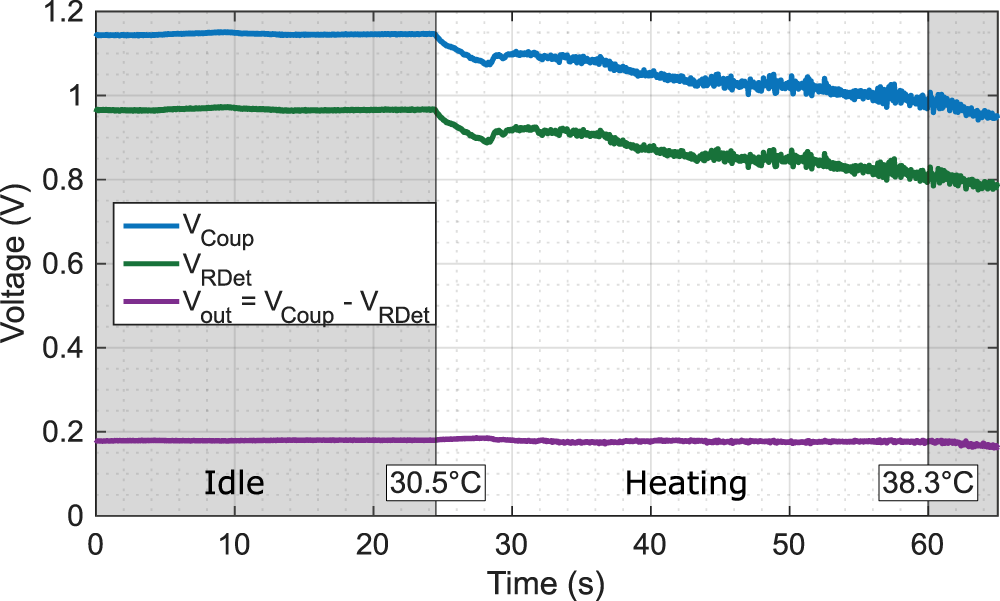
Two identical power detectors, one driven by  $P_{\mathrm{in}}$ and the other not, in very close proximity, are used to implement temperature compensation, as in [Reference Raju, Lei, Akira, Yasushi and Raja26]. For this, the coupler and detector combination is injected with a constant
 $P_{\mathrm{in}}=-15\,\mathrm{dBm}$ at
 $45\,\mathrm{GHz}$, operating well within the square-law region resulting in
 $V_{\mathrm{out}} \approx 20\,\mathrm{mV}$ induced by a constant input power. The output voltages
 $V_{\mathrm{coup}}$ and
 $V_{\mathrm{RDet}}$ are sampled every
 $12\,\mathrm{ms}$ for
 $66\,\mathrm{s}$. The measurement in Figure 9 is filtered by a Savitzky–Golay filter (3rd-order polynomial, 11-sample window length) to suppress high-frequency measurement noise that comes with the
 $12\,\mathrm{ms}$ sampling interval while preserving the thermal transient behavior and steady-state values.
Measured  $V_{\mathrm{Coup}}$ and
 $V_{\mathrm{RDet}}$ for a constant
 $P_{\mathrm{in}}=-15\,\mathrm{dBm}$ at
 $f=45\,\mathrm{GHz}$ during a heating period.

Figure 9 Long description
Voltage (V) Time (s) Legend: V subscript Coup V subscript RDet V subscript out equals V subscript Coup minus V subscript RDet Horizontal axis label: Time (s). Range: 0 to 66. Vertical axis label: Voltage (V). Range: 0 to 1.2. Text inside plot area: Idle, 30.5 degrees celsius, Heating, 38.3 degrees celsius. V subscript Coup coordinate pairs: (0, 1.15), (10, 1.16), (20, 1.16), (25, 1.15), (30, 1.10), (40, 1.05), (50, 1.02), (60, 0.99), (66, 0.95) V subscript RDet coordinate pairs: (0, 0.96), (10, 0.97), (20, 0.97), (25, 0.96), (30, 0.91), (40, 0.87), (50, 0.85), (60, 0.82), (66, 0.79) V subscript out equals V subscript Coup minus V subscript RDet coordinate pairs: (0, 0.18), (10, 0.18), (20, 0.18), (25, 0.18), (30, 0.19), (40, 0.18), (50, 0.18), (60, 0.18), (66, 0.17).
In the measurement shown in Figure 9, the detector is run at an idle measured surface temperature of  $30.5^\circ\mathrm{C}$. After
 $\approx25\,\mathrm{s}$, the chip is heated by an electric heating fan located
 $30\,\mathrm{cm}$ from the chip’s surface, as seen in Figure 5. Around the
 $60\,\mathrm{s}$ mark, the surface temperature is measured again to be
 $38.3^\circ\mathrm{C}$. While
 $V_{\mathrm{coup}}$ and
 $V_{\mathrm{RDet}}$ are affected by the increase in temperature,
 $V_{\mathrm{out}}$ remains at the constant idle level with a maximum variation of
 $\approx \pm 5\,\mathrm{mV}$, confirming the effectiveness of the temperature drift compensation.
Comparison with state-of-the-art
Several on-chip millimeter-wave power detectors have been reported in the literature, implemented in different semiconductor technologies employing different detector topologies. A direct and fair comparison is complicated by different application targets, inconsistent reporting of performance metrics, and the fact that most reported detectors are implemented without a coupler. Table 1 compares key performance metrics of reported standalone detectors. The nonuniform distributed power detector designed in this work achieves, to the best of our knowledge, the highest voltage sensitivity among reported wideband detector designs with a relative bandwidth exceeding  $100\,\mathrm{\%}$, reaching
 $10.51$–
 $45.12\,\mathrm{kV\,W^{-1}}$. Furthermore, the detector achieves broadband input matching from 2.5 to
 $92.5\,\mathrm{GHz}$, corresponding to a fractional bandwidth of
 $190\,\mathrm{\%}$. Other reported wideband designs rely on a uniform distributed detector topology [Reference Wei, Qayyum and Negra8, Reference Qayyum and Negra10, Reference Wang, Liu, Ma and Han21–Reference Qayyum, Wei and Negra23] or on resistive matching based on CMOS [Reference Qayyum and Negra9], which achieve relatively low voltage sensitivity. Among the closest integrated detectors found in the literature in terms of bandwidth and sensitivity are the two designs reported in [Reference Malotaux and Spirito14] with a sensitivity of 14 and
 $28\,\mathrm{kV\,W^{-1}}$. However, these detectors are unmatched, and the reported bandwidth does not correspond to their input matching bandwidth. Similarly, the designs reported in [Reference Zhou and Chia17, Reference Zhong, Han, Liu, Qi, Li and Wang18], although achieving a very high relative bandwidth, do not appear to have been implemented with integrating matching networks. Other comparable SiGe BiCMOS implementations trade a higher peak sensitivity of
 $91\,\mathrm{kV\,W^{-1}}$ [Reference Zheng, Gilreath, Jain and Heydari11],
 $132\,\mathrm{kV\,W^{-1}}$ [Reference Ustundag, Turkmen, Cetindogan, Kaynak and Gurbuz20],
 $772\,\mathrm{kV\,W^{-1}}$ [Reference Ustundag, Turkmen, Cetindogan, Kaynak and Gurbuz20], and
 $4\,\mathrm{MV\,W^{-1}}$ [Reference May and Rebeiz27] or a higher DR of 32 [Reference Wenger, Ng, Korndörfer, Meinerzhagen and Issakov28], 38 [Reference Stärke, Rieß, Fritsche, Carta and Ellinger29], or
 $52\,\mathrm{dB}$ [Reference Ozeren, Göyzu, Arslan and Kağan19] for a significantly reduced relative bandwidth. The DC power consumption of
 $7.79\,\mathrm{mW}$ is higher than comparable distributed implementations in CMOS, which go as low as
 $0\,\mathrm{mW}$ for a CG design [Reference Wei, Qayyum and Negra8], and comes from the higher voltage requirement of cascodes as well as the higher current draw of HBTs compared to MOSFETS, which corresponds well with the power consumption reported in [Reference Ozeren, Göyzu, Arslan and Kağan19]. The higher power consumption is additionally dominated by the output buffer at the detector’s DC output. Without it, the detector cell consumes
 $1.78\,\mathrm{mW}$. Overall, the proposed detector is the first distributed power detector demonstrated in a SiGe HBT technology and, to the best of our knowledge, achieves the highest voltage sensitivity among very wideband integrated detector designs. This makes it well suited for co-integration with broadband millimeter-wave front-end components for power-monitoring applications.
Performance comparison with the state of the art of power detectors expanded from [Reference Neff, Özat, Wörmann, Singhal, Schoch and Kallfass1]

Table 1 Long description
Rows compare power detector implementations by reference, process, topology, frequency range in gigahertz, relative bandwidth in percent, dynamic range in decibels, sensitivity in kilovolts per watt, direct current power in milliwatts, and area in square millimeters. Processes include SiGe from 90 to 250 nanometers, CMOS from 55 to 130 nanometers, and discrete implementations, with topologies including CE, CB, CS, cascode, distributed CS, distributed CG, distributed diode, and a resonant matched CS. Frequency ranges run from 0.01 to 110 gigahertz for a 65 nanometer CMOS distributed CG design, and from 30 to 300 gigahertz for a 65 nanometer CMOS distributed CS design; the highest upper frequency listed is 325 gigahertz for a 130 nanometer SiGe CE design spanning 250 to 325 gigahertz. Relative bandwidth values include 6.3 percent for a 130 nanometer SiGe cascode design spanning 76 to 81 gigahertz, and 200 percent for both a 65 nanometer CMOS resonant matched CS design spanning 0.1 to 110 gigahertz and a 65 nanometer CMOS distributed CG design spanning 0.01 to 110 gigahertz. Dynamic range values include 20 decibels for several entries, 38 decibels for a 130 nanometer SiGe cascode design spanning 100 to 130 gigahertz, 51 decibels for a discrete distributed diode design spanning 0.1 to 5.3 gigahertz, and 52 decibels for a 250 nanometer SiGe cascode design spanning 7 to 30 gigahertz; some rows leave dynamic range blank. Sensitivity values range from 0.068 to 0.7 kilovolts per watt for the 65 nanometer CMOS distributed CG entry, up to 4000 kilovolts per watt listed as part of a combined sensitivity entry for a 120 nanometer SiGe CE and LNA plus CE design spanning 84 to 103 gigahertz; several rows leave sensitivity blank. Direct current power includes 0 milliwatts for the 65 nanometer CMOS distributed CG entry, 0.068 milliwatts for a 130 nanometer SiGe cascode entry spanning 100 to 130 gigahertz, 7.2 milliwatts for a 250 nanometer SiGe cascode entry spanning 7 to 30 gigahertz, and 150 milliwatts for the discrete distributed diode entry spanning 0.1 to 5.3 gigahertz; some rows leave direct current power blank. Area values include 0.005 square millimeters for a 130 nanometer SiGe cascode entry spanning 76 to 81 gigahertz, 0.48 square millimeters for a 130 nanometer SiGe cascode entry spanning 100 to 130 gigahertz, and 864.35 square millimeters for the discrete distributed diode entry spanning 0.1 to 5.3 gigahertz; some areas include a star marker and one discrete entry leaves area blank.
Notes:
a Without pads.
b Without input matching.
c Detector without output buffer.
d Calculated from sensitivity in  $\mathrm{dB}$.
Conclusion
This work presents an extended analysis of the design and measurement of a nonuniform distributed power detector using HBT cascodes, first shown in [Reference Neff, Özat, Wörmann, Singhal, Schoch and Kallfass1]. To the best of the authors’ knowledge, this is the first distributed power detector implemented in an HBT technology. Compared to previous distributed power detector designs, stage-dependent HBT emitter dimensions are used for the detectors’ transistors to reduce DC power consumption without compromising either sensitivity or matching bandwidth. For the built-in self-test of a satellite communication linearizer, a compact broadside-coupled directional coupler is designed for operation in the Q- and V-bands. Both circuits are characterized up to  $110\,\mathrm{GHz}$ and demonstrate good agreement with EM simulation. The measured detector sensitivity closely follows the simulated frequency dependence. While the peak sensitivity is lower than that of narrowband detector implementations, the proposed approach offers a wide usable bandwidth and a significantly higher sensitivity than comparable wideband detectors. These results demonstrate that the proposed nonuniform distributed HBT detector successfully combines high sensitivity, wide bandwidth, and reduced DC power consumption. Together with the integrated temperature compensation, the presented architecture provides a promising solution for broadband millimeter-wave power sensing in future satellite communication systems.
Funding statement
The authors gratefully acknowledge the funding and support provided by the German Aerospace Center (DLR) through the project “Enhanced Self-Calibrating Amplifier Component for Space (ESCALAS)” under contract number 50RK2320. This work is supported by the Deutsche Forschungsgemeinschaft (DFG, German Research Foundation) – Project-ID 516238647 – SFB 1667/1 (ATLAS – Advancing Technologies of Very Low-Altitude Satellites).
Competing interests
The author(s) declare none.

Mark J. Neff received the B.Eng. degree in mechatronics engineering from Reutlingen University, Reutlingen, Germany, in 2021, and the M.Sc. degree in electrical engineering and information technology from the University of Stuttgart, Stuttgart, Germany, in 2024, where he is currently pursuing his Ph.D. degree at the Institute of Robust Power Semiconductor Systems (ILH). His main research interests are broadband mmW satellite communication systems and MMIC design for space applications.

Burak G. Özat received the B.S. degree in electronics engineering from Sabancı University, Istanbul, Türkiye, in 2021, and the M.Sc. degree in electrical engineering from the University of Stuttgart, Stuttgart, Germany, in 2023. He is currently a Research Assistant with the Institute of Robust Power Semiconductor Systems (ILH), University of Stuttgart. His research interests include the design of millimeter-wave MMICs, with emphasis on amplifiers, phase shifters, analog predistortion circuits, and frequency multipliers.

Ingmar Kallfass received the Dipl.-Ing. degree in electrical engineering from the University of Stuttgart, Stuttgart, Germany, in 2000, and the Dr.-Ing. degree from the University of Ulm, Ulm, Germany, in 2005, with a focus on the topic of nonlinear modeling of dispersive heterostructure field-effect transistors and their MMIC applications. In 2001, he worked as a Visiting Researcher with the National University of Ireland, Dublin, Ireland. In 2002, he joined the Department of Electron Devices and Circuits, University of Ulm, as a Teaching and Research Assistant. In 2005, he joined the Fraunhofer Institute for Applied Solid-State Physics, Freiburg im Breisgau, Germany. From 2009 to 2012, he was a Professor at the Karlsruhe Institute of Technology, Karlsruhe, Germany. Since 2013, he has held the Chair for Robust Power Semiconductor Systems at the University of Stuttgart, where his major fields of research are compound semiconductor-based circuits and systems for power and microwave electronics.







 Open access

