

INTRODUCTION
Pollution of the environment (e.g. ground and surface water; IFEN 2007) by herbicides is increasing; therefore, herbicide applications must be drastically reduced and optimized. Moreover, past simplifications of crop and herbicide rotations have led to the advent of herbicide resistance in many weed species (Powles & Yu Reference Powles, Yu, Merchant, Briggs and Ort2010), making these species more difficult and expensive to control. The recent EU directive on synthetic molecules, Registration, Evaluation, Authorisation and Restriction of Chemicals (REACH), also limited the range of herbicides available to farmers (EU 2006). Consequently, there is an increasing need for integrated cropping systems for managing weeds with little or no herbicides, basing weed control on a judicious combination of a large range of cropping system components (crop succession and the crop different management techniques). This will remain necessary even if novel weed control measures such as biocontrol, newly domesticated species or engineered weed-resistant crops become available (Gressel Reference Gressel2011). Indeed, changes in cropping systems and climate change are expected to lessen the efficiency and predictability of individual weed management measures (Rodenburg et al. Reference Rodenburg, Meinke and Johnson2011).
It is now well recognized that models that quantify the effects of crop management techniques on weed dynamics are valuable tools to design weed management strategies (Rossing et al. Reference Rossing, Meynard and van Ittersum1997; Aubertot et al. Reference Aubertot, Lescourret, Bonato, Colbach, Debaeke, Doré, Fargues, Lô-Pelzer, Loyce and Sauphanorin press). This is particularly true when designing integrated systems where a large range of interacting cropping system components must be optimized. To understand and predict the variability in effects observed for given techniques and to use these models in a large range of conditions without reparametrizing, mechanistic approaches are necessary (Colbach & Debaeke Reference Colbach and Debaeke1998; Colbach et al. Reference Colbach, Dürr, Roger-Estrade and Caneill2005; Colbach Reference Colbach2010). In this type of model, life-cycles are split into sub-processes depending on biological and physical effects of cropping systems, in interaction with the biological (e.g. weed stage) and physical (e.g. soil moisture) conditions. Such a model has already been tentatively used to evaluate crop rotations (Colbach et al. Reference Colbach, Schneider, Ballot and Vivier2010c) and to optimize crop management techniques for controlling the harmful annual grass-weed Alopecurus myosuroides Huds. (blackgrass) with little or no herbicides (Colbach et al. Reference Colbach, Kurstjens, Munier-Jolain, Dalbiès and Doré2010b).
These first applications have shown that the number of interesting management techniques is large. Moreover, they have revealed a large variability in weed infestation for a given scenario when tested with different weather scenarios. There are not only strong interactions between the different cropping system components, but also between these components and the biophysical conditions of the field. For instance, the efficiency of mechanical weeding has been shown to vary considerably with weed stage or soil moisture (Kurstjens & Perdok Reference Kurstjens and Perdok2000; Kurstjens et al. Reference Kurstjens, Perdok and Goense2000).
Consequently, the objective of the present paper was to carry out in silico experiments with AlomySys, to: (1) rank crop management components according to the resulting decrease in weed infestation and (2) study the sensitivity of the major component effects to biophysical field state variables in order to identify indicators and thresholds that could serve for future decision-rules for farmers. In order to test a large range of possible combinations of seed bank densities and crop management techniques, a global sensitivity analysis based on Monte Carlo simulations, where all input variables were made to vary randomly and simultaneously, was conducted (Saltelli et al. Reference Saltelli, Chan and Scott2000). This procedure has already been used with similar models and is useful for ranking variables over a large range of situations while taking into account the interactions between the variables (Colbach et al. Reference Colbach, Molinari and Clermont-Dauphin2004; Tricault et al. Reference Tricault, Darmency and Colbach2009). An additional, original step of the present study consisted of studying the variability in the effects of the major crop management techniques as a function of different biophysical state variables (e.g. weed densities and soil moisture).
Materials and methods
The simulation model AlomySys
The AlomySys model (Colbach et al. Reference Colbach, Busset, Yamada, Dürr and Caneill2006a, Reference Colbach, Dürr, Roger-Estrade, Chauvel and Caneillb, Reference Colbach, Chauvel, Gauvrit and Munier-Jolain2007, Reference Colbach, Kurstjens, Munier-Jolain, Dalbiès and Doré2010b) was developed for A. myosuroides Huds. (blackgrass), a harmful annual grass-weed frequently found in autumn-sown crop rotations of Atlantic European countries (Van Himme & Bulcke Reference Van Himme and Bulcke1975) and increasingly tolerant to various herbicides (Délye et al. Reference Délye, Menchari, Guillemin, Matéjicek, Michel, Camilleri and Chauvel2007; Moss et al. Reference Moss, Perryman and Tatnell2007). The input variables of AlomySys consist of:
• The daily weather data over the simulated period consisting of rainfall, mean and minimum and maximum temperatures, as well as mean soil temperatures and water potential in successive 0·01 m thick soil layers from 0 to 0·30 m depth (the maximal depth of tillage operations).
• The soil characteristics, i.e. texture, gravel content and depth.
• The initial weed infestation characterized by the total potential emergence density in the first crop of the simulation and its timing (simultaneous with crop, continuous over cropping season, late spring).
• The cropping system during the whole simulated period, comprising the crop sequence, the date of all operations (tillage, sowing, herbicides, mechanical weeding, mowing, nitrogen fertilizer, manure, harvest) and their characteristics, i.e. tool, working depth and speed, etc. for tillage and mechanical weeding, active ingredient, herbicide application rate, technology and conditions, seed sowing density, nitrogen fertilizer application rate, the rate, seed and nitrogen content of manure spreading.
• The width of the farming equipment for tilling, sowing, spraying, hoeing etc. Increasing the width reduces soil compaction and thus pre-emergent mortality during shoot elongation from the germinated seed to soil surface.
These input variables influence the annual life-cycle of blackgrass (see Supplementary Material, available at http://journals.cambridge.org/AGS), in interaction with blackgrass stages (e.g. mortality after herbicide application depends on blackgrass stage and density), crop stages (e.g. seedling survival after emergence depends on its emergence date relative to the crop emergence date) and environmental conditions (e.g. pre-emergent seedling mortality increases with the size and compaction of soil clods as well as soil dryness). The output variables considered here are, for each simulated year, the density of emerging, surviving and mature plants, weed seed production and surviving seed bank at crop harvest. AlomySys was evaluated with independent field observations and was shown to correctly predict seed survival, blackgrass emergence and multi-year dynamics in intensive and integrated cropping systems; in no-till systems, seed survival was overestimated though emergence was still predicted correctly (Colbach et al. Reference Colbach, Busset, Yamada, Dürr and Caneill2006a, Reference Colbach, Chauvel, Gauvrit and Munier-Jolain2007).
The simulation plan
The objective of the present study was to rank crop management variables according to their effects on weed infestation in a large range of weed seed bank conditions, and to identify biophysical indicators for optimizing decision-making. The simulation plan consisted in (1) simultaneously randomizing all model input variables to obtain contrasting cropping system histories, (2) running AlomySys over several years with these histories to create contrasting weed seed banks and (3) analysing the effect on weed infestation of management variables during the subsequent crop following these different weed seed banks. The crop chosen for analysing weed infestation was winter wheat, because that is the crop in which this weed species most commonly occurs. Totally 15 000 random cropping systems were run. Simulations started with 100 weed plants emerging during the first simulated crop, which was a winter wheat (to maximize initial infestation and reproduction), lasted for 20 years to maximize the difference in weed infestation between the simulated systems, and always finished with a winter wheat.
Randomization of input variables
Options for crop management variables were chosen randomly from ranges sufficiently large to comprise currently non-existing or rare, but potentially interesting, management strategies (e.g. very early sowing of summer crops to avoid summer weed emergence, cash crops sown into perennial crop cover, high-frequency tillage) as well as unusual situations resulting from organizational or climatic ‘accidents’ (e.g. very late crop sowing, very low crop densities or very low herbicide efficiencies). However, the possible ranges were kept realistic; for instance, winter crops could not be sown in spring, possible nitrogen fertilizer depended on crop types, etc. Details on the range and the probability for choosing options for the different crop management variables are given in the supplementary material available online (Supplementary Material). Soil characteristics and the width of farming equipment were chosen randomly at the onset of the simulation. Then, for each simulated year,
• The weather data set was chosen from a collection of 17 yearly weather sets from Dijon, France (5°2′E, 47°20′N, 220 m a.s.l.), ranging from 1988 to 2003.
• The crop (except the first and the last ones) was chosen among the 24 possible crops, comprising winter and spring cereals, legumes and other crops, temporary pasture as well as unsown setaside.
• The management techniques were chosen from options which varied with crop type. Ranges were made as large as possible but the logical ordering of operations was always satisfied (e.g. there was no tillage after sowing the crop).
Indicators for evaluating and optimizing crop management
The analysis of the simulated data consisted of two steps: (1) ranking the management variables of the analysed winter wheat as a function of weed infestation in this crop, (2) identifying and using biophysical indicators to optimize various management choices, i.e. timing and options (e.g. tools) of operations.
Ranking crop management variables
In each simulation, plants emerging before and during the analysed crop, plants surviving up to crop harvest, mature plants at crop harvest, total seed production and seed bank prior to seed rain at the harvest of the last year were kept as output variables for analysis. These variables were used to rank explanatory variables as a function of their impact on weed infestation. Explanatory variables comprised all crop management variables for the most recent simulated year as well as the weather for that year, soil texture and the seed bank at the onset of this year.
Biophysical indicators for optimizing management choices
In addition, a series of biophysical indicators were calculated during the simulations. These indicators consisted of weed (density, stage) and environmental variables (thermal time, cumulated rainfall, soil structure, soil water potential) ‘observed’ before management operations and, in the case of weed density indicators, during past crops. During the analysis, the variation in weed density with the various indicators was studied and optimal choices were identified as those minimizing weed density.
Statistical analysis
Ranking of crop management variables
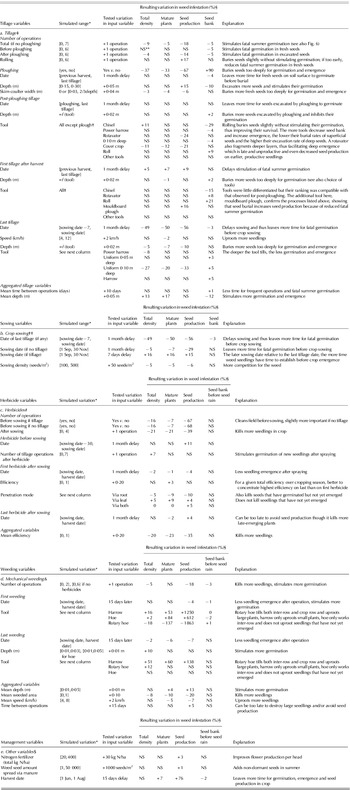
Synthetic variables for each simulated year were constructed. Each year, tillage was described by 26 variables consisting of the total number of operations if no ploughing, number of operations before and after ploughing if any, number of rolling operations; the occurrence of ploughing, its width and skim-coulter characteristics (depth, width); the dates of ploughing and the first post-ploughing, those of the first and last tillage operations; the tilling depths, tractor speeds and tools at these four major dates; mean time between operations as well as mean speed and depth for all operations (Table 1a). The variables for describing the other operations are listed in Table 1b–e. These variables resulted into 67 management variables, increased by the weather set, the seed bank characteristics and the soil texture.
Significant management techniques identified by Eqn (1) and subsequent relative variations (%) in weed infestation in winter wheat

* Probabilities for choosing options were not uniform (Supplementary Material).
† {mouldboard plough, covercrop, chisel, roll, rotavator, spring tine, power harrow, uniform 5-cm-deep, uniform 10-cm-deep, harrow}.
‡ Variables not significant at P⩽0·05 were ploughing speed, inversion, ratio, skim-coulter depth, post-ploughing speed and mean tillage speed.
§ For significant variables, relative variations are calculated from regression parameters δ i as 10δ·v−1, where v is the tested factor variation.
** NS, not significant at P⩽0·05.
†† Last tillage is carried out at sowing or during the week preceding sowing.
# Variables not significant at P⩽0·05 were efficiency and penetration mode of pre-sowing and last post-sowing herbicides as well as mean time between successive operations.
& Variables not significant at P⩽0·05 were tractor speed, tilling depth and weeded area of first mechanical weeding as well as speed and weeded area of last weeding.
$ Variables not significant at P⩽0·05 were manure type, nitrogen amount spread via manure as well as number of tillage operations after manure spreading.
To quantify the effects of crop management variables, a linear regression was used for each of the tested output variables:
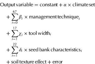 $$\eqalign{ & {\rm Output}\,{\rm variable} = {\rm constant} + \alpha \times {\rm climate}\,{\rm set} \cr &\quad + \sum\limits_{i = 0}^{67} {{\beta}_i \times {\rm management}\,{\rm technique}_i} \cr &\quad + \sum\limits_{i = 1}^{17} {\chi _i \times {\rm tool}\,{\rm width}_i} \cr &\quad + \sum\limits_{i = 1}^{22} {\delta _i \times {\rm seed}\,{\rm bank}\,{\rm characteristics}_i} \cr &\quad + {\rm soil}\,{\rm texture}\,{\rm effect} + {\rm error}} $$
where α i, βi, χi and δ i were regression parameters. All output densities were log10-transformed (after adding 1 to make possible the log-transformation of nil values) prior to analysis. Some of the input variables were quantitative (e.g. sowing density), other were qualitative variables (e.g. tools) and transformed into quantitative variables using boolean coding. For instance, the variable mechanical weeding tool with the three levels harrow, hoe and rotary hoe was transformed into distinct dummy variables equating (1,0,0) for harrow, (0,1,0) for hoe, and (0,0,1) for rotary hoe. The use of only quantitative variables made possible the use of the REG procedure of SAS (version 8.01), with the BACKWARD option to successively eliminate the least significant input variables from the regression model until only effects significant at a level of 0·05 remained. To illustrate the quantitative effects of the significant variables, the relative sensitivity of each weed variable to each input variable was calculated from regression parameters β i for a given input variation:
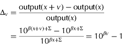 $$\Delta _v = \displaystyle{{{\rm output(}x + v{\rm )} - {\rm output(}x{\rm )}} \over {{\rm output(}x{\rm )}}} = \displaystyle{{10^{{{\beta}}(x + v) + \Sigma} - 10^{{ {\beta}}x + \Sigma}} \over {10^{{{\beta}}x + \Sigma}}} = 10^{{{\beta}}v} - 1$$
where v was the input variation, x the initial input value and Σ represents the remaining, unchanged terms of Eqn (1). Although seed bank, weather and soil texture variables were included in the present analysis, their results (as well as the analysis of additional output variables) will only be presented in the Supplementary Material available online (Supplementary Material) to focus on cropping system components.
Identification and use biophysical indicators
To identify biophysical indicators for optimizing operation dates, the targeted operation date was removed from Eqn (1). The residuals of this new regression were then analysed successively as a function of biophysical indicators, i.e. the cumulated thermal time and the cumulated rainfall since harvest or sowing until the day of the operation, soil moisture and soil structure on the operation day, as well as weed density and stage on the operation day, with a linear regression:
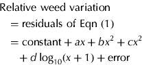 $$\eqalign{ & {\rm Relative}\ {\rm weed\ variation}\cr &\quad {\rm = residuals\ of\ Eqn\ (1)}\cr &\quad {= \rm constant} + ax + bx^2 + cx^2 \cr &\hskip6pt\quad + d\log _{10} (x + 1)+ {\rm error}} $$
where x was one of the biophysical indicators. x was introduced in different forms to allow the best representation of weed variation as a function of the indicators. Equation (3) was only applied to those data where the operation was implemented, e.g. only simulations with tillage were used to test indicators for tillage dates. To be acceptable and operational, indicators had to present the following characteristics: (1) the relationship linking relative weed density to the indicator was required to present a minimum value or decrease to a sill value for high indicator values; (2) the measurement of the indicators had to be feasible and (3) their optimization should not have any large detrimental secondary effect on other agronomic factors. Only the best indicators will be presented here; the detailed results can be found in the online appendix (Supplementary Material).
To optimize the choice of management tools, two different approaches were used. In the case of mechanical weeding, Eqn (3) was completed with a weeding tool effect as well as all interactions between the tool and the different x variables:
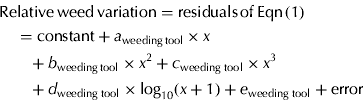 $$\eqalign{&{ \rm Relative}\,{\rm weed} \,{\rm variation} = {\rm residuals}\,{\rm of} \,{\rm Eqn}\,{\rm (1)} \cr &\quad = {\rm constant} + a_{{\rm weeding}\,{\rm tool}} \times x \cr &\quad\hskip8pt+ b_{{\rm weeding}\,{\rm tool}}\times x^2 + c_{{\rm weeding}\;{\rm tool}} \times x^3 \cr &\quad + d_{{\rm weeding}\;{\rm tool}} \times \log _{10} (x + 1) + e_{{\rm weeding}\;{\rm tool}} + {\rm error}}$$
In the case of ploughing v. no ploughing, the method was more complicated. To calculate the residuals, Eqn (1) (minus the ploughing variables) was modified by replacing the initial seed bank variables by the crops and the management techniques of the five previous years (Colbach et al., Reference Colbach, Granger and Mézière2012; Supplementary Material). Residuals were then analysed as a function of the weed infestation (i.e. mature weeds at crop harvest) in the previous crop:
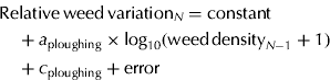 $$\eqalign{ & {\rm Relative}\,{\rm weed}\,{\rm variation}_N = {\rm constant} \cr &\quad + a_{{\rm ploughing}} \times {\rm log}_{{\rm 1}0} ({\rm weed}\,{\rm density}_{N - {\rm 1}} + {\rm 1}) \cr &\quad + c_{{\rm ploughing}} + {\rm error}} $$
Then as a function of the ratio of weed densities in the previous v. pre-previous crop:
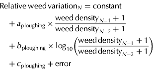 $$\eqalign{ & {\rm Relative}\,{\rm weed}\,{\rm variation}_N = {\rm constant} \cr \; &\quad + a_{{\rm ploughing}} \times \displaystyle{{{\rm weed}\,{\rm density}_{N{{\rm -} 1}} + 1} \over {{\rm weed}\,{\rm density}_{N{{\rm -} 2}} + 1}} \cr \; &\quad + b_{{\rm ploughing}} \times \log _{10} \left( {\displaystyle{{{\rm weed}\,{\rm density}_{N {{\rm -} 1}} + 1} \over {{\rm weed}\,{\rm density}_{N{{\rm -} 2}} + 1}}} \right) \cr &\quad + c_{{\rm ploughing}} + {\rm error}} $$
The same approach was used for comparing superficial v. deep ploughing (at least 0·19 m deep) and low v. high-frequency tillage (two or more tillage operations).
Results
Simulated weed infestation
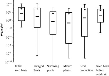
Both weed seed and plant densities varied considerably among simulations, from values close to zero to several thousand seedlings up to c. 10 000 seeds (Fig. 1). Distributions were highly skewed towards smaller values, particularly for plant densities and seed production. Mean seed bank density at the onset of the last simulated year was 6311, resulting in a mean emergence density of 755 seedlings of which only a mean proportion of 0·08 and 0·07 of seedling survived up to harvest and maturity, respectively. The latter produced a mean of 3872 seeds, which would increase seed bank by c. 60% after seed bank replenishment if there were no seed bank decrease. During the year analysed, the seed bank decreased by approximately the same value, resulting in an apparent demographic stability. Simulations, however, differed greatly: in 0·10 of the simulations, the seed bank after seed rain was divided by three in 1 year whereas in another 0·10, it was multiplied by more than 17.
Weed seed and plant densities at different stages throughout the annual simulation. Box-and-whisker plots show 1, 10, 50, 90 and 99% percentiles, +shows mean values.

Contribution of the various simulation factors
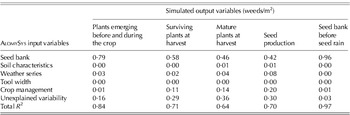
Plant densities mostly depended on initial seed bank characteristics, though the contribution of the latter decreased with the ‘lateness’ of the stage, i.e. the contribution was lower for mature than for emerged plants (Table 2). Seed production depended even less on initial seed bank. However, the magnitude of the final seed bank before the new seed rain depended almost entirely on seed bank characteristics. Soil characteristics were negligible, while weather only explained 0·02–0·08 of above-ground weed densities, with a slight increase from ‘early’ (i.e. emerged plants) to ‘late’ stages (i.e. seed production). Its impact on the final seed bank was small. The effect of crop management increased from 0·01 for the earliest to 0·20 for the latest post-emergence stage; it was negligible for final seed bank. The effect of the width of the different agricultural tool was never significant.
Variability in simulated weed output variables in winter wheat explained by AlomySys input variables. Partial and total R 2 of Eqn (1)

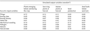
Among the crop management variables, tillage and, to a lesser degree, mechanical weeding were most important for determining the total emergence density (Table 3). These are the techniques that mostly determine seed germination via seed burial, dormancy breaking and the stimulation of germination flushes; they also influence emergence via their effect of pre-emergent seedling mortality due to seed depth and soil compaction. Sowing date was important because it determined the position of the weed seed dormancy cycle relative to the crop cycle. Manure had a slight effect through adding non-dormant seeds to the soil, thus boosting additional germination. Nitrogen fertilizer did not have any effect on emergence timing because it did not affect the soil seed bank processes, only the number and dormancy of the next weed seed rain. Sowing density and harvest did not influence emergence because they did not influence pre-emergent processes. Herbicides had a very slight effect because root-entering herbicides could kill seedlings that had yet to emerge.
Variability in simulated weed output variables explained by crop management variables. Proportion of partial R2 of Eqn (1) due to crop management
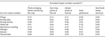
When looking at surviving and mature plants at harvest and their seed production, techniques affecting post-emergence survival became much more significant, with herbicides and, again, mechanical weeding now the dominant techniques (Table 3). Seed density also became important, because of crop-weed competition. Harvest date was the most important management technique for determining the variability in weed seed production because it determined the time left to weed plants to mature before their destruction by the harvest equipment.
The situation was very different for the seed bank found at crop harvest, prior to the addition of the newly produced seeds. This seed bank almost entirely depended on tillage and, to a small degree, on mechanical weeding, via their effect of seed burial, dormancy breaking and germination stimulation. The only other relevant technique was the date of the crop harvest, timing the moment at which the surviving seed bank was calculated.
The effect of crop management variables
The crop management variables that presented a significant effect on at least one of the weed variables are listed in Table 1, together with a quantitative estimation of this effect as well as its probable cause. Variations were similar for plants and seed production in crops though effects were usually most frequent and variations largest for seed production. The variations in surviving seed bank (prior to the new seed rain) were usually opposite to those in plants, pointing to germination as a major process, emptying the former and resulting in the increase in the latter after subsequent pre-emergent growth. Only a few changes in management techniques (e.g. increasing the number of tillage operations) decreased both weed plants and surviving seed bank. These were due to an increase in fatal summer germination, i.e. in the germination of seeds that did not emerge or resulted in seedlings that were killed before crop sowing. The effect of some characteristics was stable, for instance the number of herbicide sprayings, whether applied before or after crop sowing, always decreased weed infestation. For other techniques, the effect depended on the date of the operation, for instance tools which provided deep tillage and/or burying of weeds should be avoided for early tillage because they reduce fatal summer germination whereas they would be best for the last tillage prior to or at the time of crop sowing, because they bury weeds too deeply for them to germinate and emerge during the crop.
Identifying biophysical indicators for decision-making
Optimizing the choice of tools and dates as a function of biophysical indicators
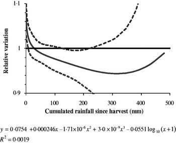
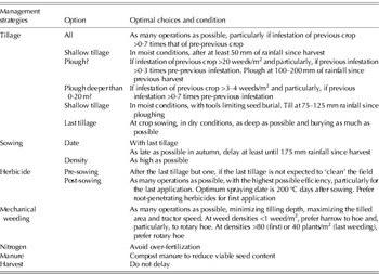
Ploughing date could best be optimized by taking into account the cumulated rainfall since previous harvest (Fig. 2). Relative weed seed production steadily decreased when ploughing was delayed until 200 mm of cumulated rainfall after previous harvest, because this left more time for fatal summer germination before burial, particularly from fresh seeds. After that date, the effect became variable, with an increasing risk of weed infestation because seeds excavated and stimulated by ploughing and subsequent tillage presented a higher probably of emerging after crop sowing. The dates of first, post-ploughing and last tillage operations could also be optimized with cumulated rainfall (Supplementary Material) for details and synthesis in Table 4). Delaying the first tillage after optimum timing of 50 mm did not increase weed density.
Indicator for optimizing mouldboard ploughing date. Relative weed seed production in winter wheat as a function of cumulated rainfall from previous harvest to ploughing day (continuous line=regression, dashed lines=95% confidence interval). Results of Eqn (3).

Summary of advice for controlling autumnal grass weeds in winter wheat

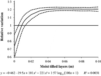
The rainfall indicator was better than the number of days or thermal time since harvest because it also integrated the seed requirement for soaking to germinate and that rainfall also contributes to breaking dormancy in fresh seeds. Relative weed seed production was also negatively correlated with the number of tilled moist layers (i.e. with a water potential above the base value for germination) for all but the last tillage. These relationships cannot be used directly for decision-making because soil water potential is too difficult to measure. However, this indicator revealed that the last tillage should be carried out in conditions as dry as possible because weed risk increased steadily with soil moisture (Fig. 3), which favoured germinating seeds emerging in the crop.
Variation of weed seed production as a function of soil moisture before the last tillage preceding winter wheat (continuous line=regression with, dashed lines=95% confidence interval).

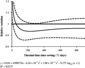
None of the tested indicators was able to optimize sowing date. The timing of herbicide spraying was best optimized with thermal time, though a similar but less significant relationship could be obtained for cumulated rainfall (Supplementary Material). Spraying was best delayed until 200 °C days after sowing (Fig. 4) to leave more time for seedlings to emerge and be killed by the herbicide. After 300 °C days, the weeds were too large and numerous to be destroyed. There was no significant difference between herbicides with different penetration modes.
Indicator for optimizing the timing of the first herbicide after crop sowing. Relative weed seed production in winter wheat as a function of thermal time (base 0 °C) from crop sowing to operation day (continuous line=regression with, dashed lines=95% confidence interval). Results of Eqn (3).

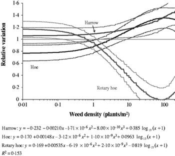
In the case of mechanical weeding, both tools and timing could be optimized. Weed density was the indicator with the highest explanatory power (i.e. highest R 2) though thermal time and cumulated weed foliar stage could also be used (Supplementary Material). When weed densities were low (<1 plant/m2 approximately), the optimal tools for both first and last weeding were hoeing and, to a lesser degree, harrowing; at that time, plants were still small and the proportion of seedlings yet to emerge was high, which were the stages best uprooted by these tools (Fig. 5). At greater densities, a rotary hoe was the optimal tool because it also uprooted large weeds, but its use was most effective at weed densities below 80 and 40 plants/m2 for the first and last operations, respectively.
Indicator for optimizing the date and tool of the first mechanical weeding operation. Relative weed seed production in winter wheat as a function of weed density on the operation day (continuous line=regression with, dashed lines=95% confidence interval). Results of Eqn (4).

Optimizing tillage choices as a function of past weed infestations
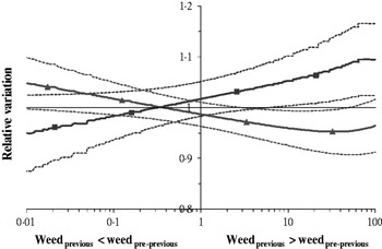
Although ploughing was identified as the usual optimal choice over no-ploughing (Table 1a), analyses taking account of past weed infestation showed that this was only true when the weed infestation in the previous crop exceeded c. 20 plants/m2 (Supplementary Material). Moreover, ploughing was only the best option when the infestation of the previous crop exceeded c. 0·3 times that of the pre-previous crop (Fig. 6).
Variation of weed seed production in ploughed (▲) and un-ploughed (■) winter wheat as a function of the ratio of the weed densities in the previous v. pre-previous crop (continuous line=regression with, dashed lines=95% confidence interval). Results of Eqn (6), R 2=0·011.

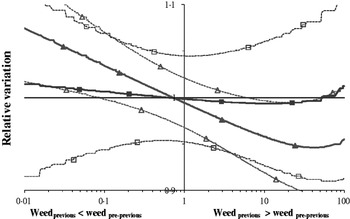
The situation was even more complicated for ploughing depth. The initial analysis showed weed infestation to increase with ploughing depth (Table 1a). The analysis as a function of weed density in the previous crop showed this to be true only when this density was lower than c. 3–4 plants/m2 (Supplementary Material). In addition, deep ploughing was best when weeds in the previous crop exceeded c. 0·7 times those in the pre-previous crop (Fig. 7). Similarly, high-frequency tillage (two or more operations) was shown to be most interesting when the previous weed infestation exceeded c. 0·4 times the pre-previous infestation (Supplementary Material).
Variation of weed seed production in deeply (deeper than 0·19 m: ▲, △) and superficially ploughed (less than 0·19 m: ■, □) winter wheat as a function of the ratio of the weed densities in the previous v. pre-previous crop (continuous line=regression with, dashed lines=95% confidence interval). Results of Eqn (6), R 2=0·011.

Discussion
Implications for designing grass weed management strategies
The first major result of the present study was the quantitative, synthetic ranking of the crop management effects in the short-term, identifying the optimal choices for each management technique (Table 4). These are particularly interesting for techniques with contradicting effects, strong interactions with the environment, and many possible choices such as tillage. Other conclusions are less original, e.g. crop sowing density, but confirm reports from field trials and surveys (e.g. Chauvel et al. Reference Chauvel, Guillemin, Colbach and Gasquez2001). But even for a priori evident advice such as ‘maximize herbicide efficiency’, new indications could be identified, such as the focus on the last spraying rather than the first. Similar advice on grass weed management has already been compiled in previous reports (e.g. Moss & Clarke Reference Moss and Clarke1994), but the present management rules are much more detailed (e.g. distinction of different tillage types), quantify effects (e.g. maximize efficiency of the last rather than earlier herbicide sprayings) and adapt the rules to weed (e.g. density prior to operation) and environmental conditions (e.g. rainfall).
However, the present advice is conditional to the model quality, although many aspects of the model have been satisfactorily evaluated, e.g. tillage and sowing date (Colbach et al. Reference Colbach, Busset, Yamada, Dürr and Caneill2006a, Reference Colbach, Chauvel, Gauvrit and Munier-Jolain2007). Moreover, most of the major effects identified in the present paper are consistent with previous field observations and should therefore be robust in a large range of field conditions, e.g. the decrease in blackgrass or similar species in case of mouldboard ploughing or delayed sowing (Schneider et al. Reference Schneider, Walter, Koch and Kemmer1984; Chauvel et al. Reference Chauvel, Guillemin, Colbach and Gasquez2001; Moss et al. Reference Moss, Perryman and Tatnell2007; Cirujeda & Taberner Reference Cirujeda and Taberner2009). Literature reports on minor factors such as nitrogen fertilizer effects are partial and inconsistent (e.g. blackgrass biomass decrease in pot-grown weed-wheat mixtures: Naylor (Reference Naylor1972b); blackgrass seed production increase in cereal crops: Chauvel Reference Chauvel1996; Chauvel et al. Reference Chauvel, Angonin, Colbach, van Ittersum, Venner and van de Geijn1996) and make it difficult to check the robustness of the present results. Similarly, the advice on optimal tools for mechanical weeding is only valid if a rotary hoe does indeed fail to destroy seedlings that have not yet emerged, as assumed by AlomySys. Further tests, of the model itself and of the present advice, are therefore necessary.
Though the present methodology has already been used with other weed dynamics models (Colbach et al. Reference Colbach, Molinari and Clermont-Dauphin2004; Tricault et al. Reference Tricault, Darmency and Colbach2009), the present study could improve the initial approach with the integration of biophysical indicators for optimizing management strategies (e.g. delay the first tillage until 50 mm rainfall after harvest). This original approach contributes to improving understanding of the variability in the crop management effects and to making management advice much more robust, optimizing it for different biophysical conditions. Moreover, these flexible rules are much closer to the actual farming decision processes (Aubry et al. Reference Aubry, Papy and Capillon1998). Indeed, operations are usually not executed at a fixed date, irrespective of conditions, but depend on diverse factors such as weather, soil moisture, crop and weed growth stages, trafficability restrictions, competition with other farm work etc. (Macé et al. Reference Macé, Morlon, Munier-Jolain and Quéré2007).
The present study demonstrated the enormous importance of interactions, not only among crop management techniques but also between techniques and biophysical conditions in the field. The latter have been partially integrated into the present, innovative approach, representing the variability in management effects on weed infestation as a function of different biophysical indicators. However, a large proportion of variability remained unexplained, even when integrating these indicators. It is possible that a part of this variability is not actually pertinent and an artefact of the present simulation plan, where all management variables were randomized. Many combinations were probably highly improbable in farming reality. Consequently, more focused simulation studies are necessary, starting with existing or probable cropping systems and testing prospective scenarios based on the present guidelines and biophysical indicators. Such an approach has already been attempted with fixed-date scenarios (Colbach et al. Reference Colbach, Granger and Munier-Jolain2009, Reference Colbach, Schneider, Ballot and Vivier2010c, Reference Colbach, Granger and Mézièrein press; Mézière et al. Reference Mézière, Granger, Boissinot and Colbach2011) but to the best of our knowledge, not yet with biophysical indicators.
Methodology
Though the present study developed an original addition to existing sensitivity analysis methods with the integration of biophysical indicators, it presents several major disadvantages. Firstly, the effect of crop management was only studied in a single crop, albeit the one where the studied weed species is most frequent and harmful (Van Himme & Bulcke Reference Van Himme and Bulcke1975). Moreover, variable effects were represented as linear, with either a positive or negative effect. Actually, as the indicator analysis showed, effects are often more complex, e.g. weed infestation first decreased when tillage was delayed after harvest and later increased the closer to crop sowing the operation was executed. Lastly, the effect was only studied in the short-term, over 1 year. This is a considerable short-coming because weed seeds survive for several years, even short-lived grass species such as blackgrass (Lonchamp et al. Reference Lonchamp, Chadoeuf, Barralis and Bourlier1984). The 1-year step thus neglected one of the major, known effects on weed dynamics, i.e. crop succession and the long-term effects of crop management (Chauvel et al. Reference Chauvel, Guillemin, Colbach and Gasquez2001; Bohan et al. Reference Bohan, Powers, Champion, Haughton, Hawes, Squire, Cussans and Mertens2011). This is, for instance, the case of seed burial by tillage (e.g. Naylor Reference Naylor1972a) partially seen here via increases in seed bank survival, of seed addition by manure (Pleasant & Schlather Reference Pleasant and Schlather1994; Miyazawa et al. Reference Miyazawa, Tsuji, Yamagata, Nakano and Nakamoto2004), of the primary dormancy of newly produced seeds due to modifications in emergence and maturity dates as well as nitrogen fertilization (Colbach & Dürr Reference Colbach and Dürr2003; Swain et al. Reference Swain, Hughes, Cook and Moss2006).
The 1-year scale of the present analysis was a deliberate decision, to focus on interactions with biophysical field state variables. Long-term effects and interactions were studied in a companion paper, confirming most of the crop management effects observed in the present paper (Colbach et al. Reference Colbach, Granger and Mézière2012).
Conclusion
The main new outcomes from the present study were the development of detailed and quantitative management rules for weed management adapted to weed (e.g. weed density prior to weeding) and environmental conditions (e.g. rainfall), leading to the identification of biophysical indicators pertinent for optimizing management decisions. From a methodology perspective, the present study adapted an existing method of sensitivity analysis for complex, multi-variate cropping system models to not only rank and quantify crop management effects, but also appreciate their variability as a function of biophysical field state variables.
To progress in the development of integrated weed management, additional simulation studies are necessary to study management effects and interactions in more contrasting and representative cropping system types, focusing on the trade-off between different techniques. For instance, how many more time-consuming (e.g. tillage) or yield-decreasing modifications (e.g. delayed sowing date) are necessary to compensate the elimination of a given herbicide application. Or, from a different perspective, how many herbicide applications become superfluous in a diversified rotation with frequent mouldboard ploughing. The latter question will necessitate additional preliminary sensitivity analyses which are presented in a companion paper (Colbach et al. Reference Colbach, Granger and Mézière2012).
The present study considers only a single weed species, albeit a frequent and harmful one. The results could be tentatively extrapolated to species with similar traits (e.g. Lolium) but this would only be possible for a small number of species. Though the present authors have already carried out a similar sensitivity analysis with a very different weed (i.e. the spring-emerging broad-leaved crop relative, Beta vulgaris spp. vulgaris, Tricault et al. Reference Tricault, Darmency and Colbach2009), truly multi-specific weed dynamics models (Colbach et al. Reference Colbach, Gardarin, Munier-Jolain, Bastiaans, Bohren, Christensen, Gerowitt, Hatcher, Krähmer, Kudsk, Melander, Pannacci, Rubin, Streibig, Tei, Thompson, Torresen and Vurro2010a; Gardarin et al. Reference Gardarin, Dürr and Colbachin press) will be necessary to design integrated cropping systems.
SUPPLEMENTARY MATERIAL REFERENCE
Supplementary Material. Additional information and results for the paper ‘Using a sensitivity analysis of a weed dynamics model to develop sustainable cropping systems. I. Annual interactions between crop management techniques and biophysical field state variables’. Journal of Agricultural Science, Cambridge 2012; Supplementary Material (available at http://journals.cambridge.org/AGS).
The present work was financed by INRA and ANR SYSTERRA ADVHERB (ANR-08-STRA-02).