A. Preliminaries and Definitions

We begin with some preliminaries, and we consider the following notations: Given two entities $ \boldsymbol{Y}={\left({Y}_1,{Y}_2\right)}^{\prime } $ , we let $ {\boldsymbol{Y}}_t\equiv {\left({Y}_{1,t},{Y}_{2,t}\right)}^{\prime } $ collect their returns at time $ t $ . In the context of backtesting systemic risk, $ {Y}_{1,t} $ is the stock return of a financial institution, whereas $ {Y}_{2,t} $ is the system return which is usually proxied by the return of a market index. We let $ {\Omega}_{t-1} $ collect the information available at time $ t-1 $ , and we denote by $ {F}_Y\left(\cdot |{\Omega}_{t-1}\right) $ the joint distribution function of $ {\boldsymbol{Y}}_t $ given $ {\Omega}_{t-1} $ , such that we have for any $ \boldsymbol{y}=\left({y}_1,{y}_2\right)\in {\mathrm{\mathbb{R}}}^2 $ , $ {F}_Y\left(\boldsymbol{y}|{\Omega}_{t-1}\right)=\mathrm{\mathbb{P}}\left({Y}_{1,t}\le {y}_1,{Y}_{2,t}\le {y}_2|{\Omega}_{t-1}\right) $ . Similarly, we let $ {F}_{Y2}\left(\cdot |{\Omega}_{t-1}\right) $ denote the marginal distribution of $ {Y}_{2,t} $ given $ {\Omega}_{t-1} $ , such that we have for any $ {y}_2\in \mathrm{\mathbb{R}} $ , $ {F}_{Y2}\left({y}_2|{\Omega}_{t-1}\right)=\mathrm{\mathbb{P}}\left({Y}_{2,t}\le {y}_2|{\Omega}_{t-1}\right) $ . For notational simplicity, we drop “almost surely” in all equalities involving random variables.

We now introduce the definitions of systemic risk measures MES and CoVaR. Formally, for a given $ \alpha \in \left[0,1\right] $ , the MES of an institution at time $ t $ is defined as

(1) $$ {MES}_{Y1,t}\left(\alpha \right)=\unicode{x1D53C}\left({Y}_{1,t}|{Y}_{2,t}\le {VaR}_{Y2,t}\left(\alpha \right);{\Omega}_{t-1}\right), $$

where $ {VaR}_{Y2,t}\left(\alpha \right) $ verifies $ {VaR}_{Y2,t}\left(\alpha \right)={F}_{Y2}^{-1}\left(\alpha |{\Omega}_{t-1}\right) $ . Because $ \alpha $ is typically specified at a small value such as 5%, the event $ {Y}_{2,t}\le {VaR}_{Y2,t}\left(\alpha \right) $ captures the left tail distressed system condition. Thus, $ {MES}_{Y1,t}\left(\alpha \right) $ quantifies the expected performance of a financial institution given that the system is in distress. The CoVaR definition shares the similarity that it also emphasizes the distress system condition. For a given $ \beta \in \left[0,1\right] $ , the CoVaR of an institution at time $ t $ is the quantity $ {CoVaR}_{Y1,t}\left(\beta, \alpha \right) $ verifying the following equation:

(2) $$ \mathrm{\mathbb{P}}\left({Y}_{1,t}\le {CoVaR}_{Y1,t}\left(\beta, \alpha \right)|{Y}_{2,t}\le {VaR}_{Y2,t}\left(\alpha \right);{\Omega}_{t-1}\right)=\beta . $$

The CoVaR definition (2) differs slightly from that in Adrian and Brunnermeier (Reference Adrian and Brunnermeier2016), where the main difference is the use of an inequality (instead of an equality) for the conditioning event (i.e., $ {Y}_{2,t}\le {VaR}_{Y2,t}\left(\alpha \right) $ ). Our definition allows for losses beyond $ {VaR}_{Y2,t}\left(\alpha \right) $ and is in line with the backtesting literature (see, e.g., Girardi and Ergün (Reference Girardi and Ergün2013), Banulescu-Radu et al. (Reference Banulescu-Radu, Hurlin, Leymarie and Scaillet2021)). Besides, we note $ {CoVaR}_{Y1,t}\left(\beta, \alpha \right) $ verifies $ {CoVaR}_{Y1,t}\left(\beta, \alpha \right)={F}_{Y_1\mid {Y}_2\le {VaR}_{Y2}\left(\alpha \right)}^{-1}\left(\beta |{\Omega}_{t-1}\right) $ , where $ {F}_{Y_1\mid {Y}_2\le {VaR}_{Y2}\left(\alpha \right)}\left(\cdot |{\Omega}_{t-1}\right) $ is the conditional distribution of $ {Y}_{1,t} $ given $ {Y}_{2,t}\le {VaR}_{Y2,t}\left(\alpha \right) $ and $ {\Omega}_{t-1} $ . In other words, $ {CoVaR}_{Y1,t}\left(\beta, \alpha \right) $ measures an institution’s $ \beta $ -quantile return given that the system is in distress.

In practice, systemic risk measures are typically estimated and forecasted from a parametric model specified by academics, risk managers, or regulators. For instance, Brownlees and Engle (Reference Brownlees and Engle2017) and Banulescu-Radu et al. (Reference Banulescu-Radu, Hurlin, Leymarie and Scaillet2021) consider the dynamic conditional correlation (DCC) specification to model and forecast systemic risk. Therefore we suppose, along with other risk measures of interest, $ {VaR}_{Y2,t}\left(\alpha \right)\equiv {VaR}_{Y2,t}\left(\alpha, {\boldsymbol{\theta}}_0\right)={F}_{Y2}^{-1}\left(\alpha |{\Omega}_{t-1},{\boldsymbol{\theta}}_0\right) $ and $ {CoVaR}_{Y1,t}\left(\beta, \alpha \right)\equiv {CoVaR}_{Y1,t}\left(\beta, \alpha, {\boldsymbol{\theta}}_0\right)={F}_{Y_1\mid {Y}_2\le {VaR}_{Y2}\left(\alpha \right)}^{-1}\left(\beta |{\Omega}_{t-1},{\boldsymbol{\theta}}_0\right) $ , are computed from a parametric model with true but unknown $ p $ -dimensional parameter vector $ {\boldsymbol{\theta}}_0\in {\varTheta}_0\subseteq \varTheta \subset {\mathrm{\mathbb{R}}}^p $ .

To backtest systemic risk measures, BHLS define a violation risk indicator based on the ex post risk sequence $ \left\{{CoVaR}_{Y1,t}\left(\beta, \alpha, {\boldsymbol{\theta}}_0\right),{VaR}_{Y2,t}\left(\alpha, {\boldsymbol{\theta}}_0\right)\right\} $ evaluated at a specified ( $ \alpha $ , $ \beta $ ) level, namely

$$ {h}_t\left(\alpha, \beta, {\boldsymbol{\theta}}_0\right)\equiv \unicode{x1D7D9}\left[\left({Y}_{1,t}\le {CoVaR}_{Y1,t}\left(\beta, \alpha, {\boldsymbol{\theta}}_0\right)\right)\cap \left({Y}_{2,t}\le {VaR}_{Y2,t}\left(\alpha, {\boldsymbol{\theta}}_0\right)\right)\right]. $$

Next, by identifying the MES-CoVaR relation (i.e., $ {MES}_{Y1,t}\left(\alpha \right)={MES}_{Y1,t}\left(\alpha, {\boldsymbol{\theta}}_0\right)={\int}_0^1{CoVaR}_{Y1,t}\left(\beta, \alpha, {\boldsymbol{\theta}}_0\right)\mathrm{d}\beta $ ), we obtain as with BHLS the risk indicator for MES

$$ {\displaystyle \begin{array}{c}{H}_t\left(\alpha, {\boldsymbol{\theta}}_0\right)\equiv {\int}_0^1{h}_t\left(\alpha, \beta, {\boldsymbol{\theta}}_0\right)\mathrm{d}\beta \\ {}=\unicode{x1D7D9}\left[{F}_{Y_2}\left({Y}_{2,t}|{\Omega}_{t-1},{\boldsymbol{\theta}}_0\right)\le \alpha \right]\times \left[1-{F}_{Y_1\mid {Y}_2\le {VaR}_{Y2}\left(\alpha, {\boldsymbol{\theta}}_0\right)}\left({Y}_{1,t}|{\Omega}_{t-1},{\boldsymbol{\theta}}_0\right)\right],\end{array}} $$

where the second equality follows by probability integral transform. The idea of backtesting risk measures using their “respective” risk indicators is standard in the literature. For instance, $ {h}_t\left(\alpha, \beta, {\boldsymbol{\theta}}_0\right) $ and $ {H}_t\left(\alpha, {\boldsymbol{\theta}}_0\right) $ are analogous to risk indicators used in backtesting, respectively, the value-at-risk measure (see, e.g., Berkowitz, Christoffersen, and Pelletier (Reference Berkowitz, Christoffersen and Pelletier2011)) and the expected shortfall measure (see, e.g., Du and Escanciano (Reference Du and Escanciano2017)). By the same reasoning, BHLS propose to use $ {h}_t\left(\alpha, \beta, {\boldsymbol{\theta}}_0\right) $ to backtest CoVaR at a specified $ \left(\alpha, \beta \right) $ level, and to use $ {H}_t\left(\alpha, {\boldsymbol{\theta}}_0\right) $ to backtest MES at a specified $ \alpha $ level.

To backtest risk measures, the literature generally relies on exploiting the martingale difference sequence (mds) property of risk indicators. The mds property of $ {h}_t\left(\alpha, \beta, {\boldsymbol{\theta}}_0\right) $ and $ {H}_t\left(\alpha, {\boldsymbol{\theta}}_0\right) $ can be noted as follows: First, by Bayes theorem, we have $ \mathrm{\mathbb{P}}\left({h}_t\left(\alpha, \beta, {\boldsymbol{\theta}}_0\right)=1|{\Omega}_{t-1}\right)=\alpha \beta $ . It follows from definition (2) that $ {h}_t\left(\alpha, \beta, {\boldsymbol{\theta}}_0\right) $ follows the Bernoulli $ \left(\alpha \beta \right) $ distribution, and that the ex post centered indicator $ \left\{{h}_t\left(\alpha, \beta, {\boldsymbol{\theta}}_0\right)-\alpha \beta \right\} $ is a mds at the specified $ \left(\alpha, \beta \right) $ level. Second, by Fubini’s theorem, we note that the mds property of $ \left\{{h}_t\left(\alpha, \beta, {\boldsymbol{\theta}}_0\right)-\alpha \beta \right\} $ is preserved by integration, and that the mean of $ {H}_t\left(\alpha, {\boldsymbol{\theta}}_0\right) $ is given by $ \alpha /2 $ . Therefore, $ \left\{{H}_t\left(\alpha, {\boldsymbol{\theta}}_0\right)-\alpha /2\right\} $ is also a mds at the specified $ \alpha $ level, i.e.,

(3) $$ \unicode{x1D53C}\left({H}_t\left(\alpha, {\boldsymbol{\theta}}_0\right)-\alpha /2|{\Omega}_{t-1}\right)=0. $$

Notice that by definition of $ {H}_t\left(\alpha, {\boldsymbol{\theta}}_0\right) $ and Fubini’s theorem, we have $ \unicode{x1D53C}\left({H}_t\left(\alpha, {\boldsymbol{\theta}}_0\right)|{\Omega}_{t-1}\right)={\int}_0^1\unicode{x1D53C}\left({h}_t\left(\alpha, \beta, {\boldsymbol{\theta}}_0\right)|{\Omega}_{t-1}\right)\mathrm{d}\beta $ . It follows that for equation (3) to hold, the CoVaR indicator $ {h}_t\left(\alpha, \beta, {\boldsymbol{\theta}}_0\right) $ must be properly modeled not just at a specified $ \beta $ but instead for all $ \beta \in \left[0,1\right] $ . This is a complementary observation to existing literature. It implies that by examining the MES measure using $ {H}_t\left(\alpha, {\boldsymbol{\theta}}_0\right) $ at a specified $ \alpha $ level, we are simultaneously examining the CoVaR measure using $ {h}_t\left(\alpha, \beta, {\boldsymbol{\theta}}_0\right) $ , at the same $ \alpha $ level, but for all $ \beta \in \left[0,1\right] $ . Thus, we propose to examine MES and CoVaR jointly based on the mds property of $ {H}_t\left(\alpha, {\boldsymbol{\theta}}_0\right) $ , which gives a general procedure (i.e., one that can be conveniently used to detect inadequate systemic risk estimated using either CoVaR or MES). Our procedure is in line with the “better-safe-than-sorry” philosophy advocated by major regulatory body such as the European Central Bank.Footnote ¹ This is because, in practice, the CoVaR and MES of a financial institution are usually estimated and forecasted by the same risk model (see, e.g., Banulescu-Radu et al. (Reference Banulescu-Radu, Hurlin, Leymarie and Scaillet2021)). By backtesting MES and CoVaR jointly, we require the risk model to adequately produce both estimates. This imposes a more stringent requirement on institutional risk modeling which in turn promotes a safer empirical practice.

B. The Main Hypotheses

Therefore, to backtest MES and CoVaR, we focus on the mds $ \left\{{H}_t\left(\alpha, {\boldsymbol{\theta}}_0\right)-\alpha /2\right\} $ to obtain as with the broader backtesting literature the zero mean condition (i.e., $ \unicode{x1D53C}\left({H}_t\left(\alpha, {\boldsymbol{\theta}}_0\right)\right)-\alpha /2=0 $ ) and the zero autocovariance condition (i.e., $ \unicode{x1D53C}\left[\left({H}_t\left(\alpha, {\boldsymbol{\theta}}_0\right)-\unicode{x1D53C}\left({H}_t\left(\alpha, {\boldsymbol{\theta}}_0\right)\right)\right)\times \left({H}_{t-j}\left(\alpha, {\boldsymbol{\theta}}_0\right)-\unicode{x1D53C}\left({H}_{t-j}\left(\alpha, {\boldsymbol{\theta}}_0\right)\right)\right)\right]=0 $ for all $ j\ge 1 $ ), which are sometimes referred to as the unconditional hypothesis and the independence hypothesis, respectively (see, e.g., Christoffersen (Reference Christoffersen1998), Du and Escanciano (Reference Du and Escanciano2017), and Banulescu-Radu et al. (Reference Banulescu-Radu, Hurlin, Leymarie and Scaillet2021)).

To ensure asymptotic full detection power against both hypotheses, we construct a statistical framework that considers both the unconditional and the independence conditions. This is achieved by first applying $ \unicode{x1D53C}\left({H}_t\left(\alpha, {\boldsymbol{\theta}}_0\right)\right)=\alpha /2 $ , for all $ t $ , in the autocovariance $ \gamma (j) $ and autocorrelation $ \rho (j) $ functions

(4) $$ \gamma (j)\equiv \unicode{x1D53C}\left[\left({H}_t\left(\alpha, {\boldsymbol{\theta}}_0\right)-\alpha /2\right)\times \left({H}_{t-j}\right(\alpha, {\boldsymbol{\theta}}_0\left)-\alpha /2\right)\right],\hskip1em \rho (j)=\gamma (j)/\gamma (0). $$

Then, based on $ \rho (j) $ , we specify the main hypotheses of the article

$$ {\unicode{x210D}}_0:\rho (j)=0\hskip0.62em \mathrm{f}\mathrm{o}\mathrm{r}\hskip0.42em \mathrm{a}\mathrm{l}\mathrm{l}\hskip0.42em j\ge 1,\hskip1em {\unicode{x210D}}_1:\rho (j)\ne 0\hskip0.62em \mathrm{f}\mathrm{o}\mathrm{r}\hskip0.62em \mathrm{a}\mathrm{n}\mathrm{y}\hskip0.62em j\ge 1. $$

By construction, our hypotheses take into account jointly both the zero mean condition and the zero autocovariance condition. A statistical test consistent against divergence from $ {\mathrm{\mathbb{H}}}_0 $ (i.e., with asymptotic unit power under $ {\mathrm{\mathbb{H}}}_1 $ ) would be consistent against both conditions. This is confirmed using the new backtests in our simulation study.

In practice, we do not observe $ {H}_t\left(\alpha, {\boldsymbol{\theta}}_0\right) $ and $ \rho (j) $ , but we can estimate them using the observed sample $ {\left\{{Y}_{1,t},{Y}_{2,t}\right\}}_{t=1}^{T+n} $ . In this aspect, we note that the fundamental notion of backtesting is about examining the quality of a sequence of forecasts (using, e.g., $ {\mathrm{\mathbb{H}}}_0 $ ). This calls for a forecasting scheme. For meaningful comparison, we use as with BHLS the “fixed forecasting estimation scheme.” That is, we first use an in-sample return data from $ t=1 $ to $ t=T $ (i.e., $ {\left\{{Y}_{1,t},{Y}_{2,t}\right\}}_{t=1}^T $ ) to estimate $ {\boldsymbol{\theta}}_0 $ , by, e.g., $ {\hat{\boldsymbol{\theta}}}_T $ , where $ {\hat{\boldsymbol{\theta}}}_T $ is a consistent estimator for $ {\boldsymbol{\theta}}_0 $ , with the asymptotic variance of $ \sqrt{T}\left({\hat{\boldsymbol{\theta}}}_T-{\boldsymbol{\theta}}_0\right) $ given by $ \varSigma $ . Then, using $ {\hat{\boldsymbol{\theta}}}_T $ and the out-sample return data observed from $ t=T+1 $ to $ t=T+n $ (i.e., $ {\left\{{Y}_{1,t},{Y}_{2,t}\right\}}_{t=T+1}^{T+n} $ ), we forecast and compute $ {\{{H}_t(\alpha, {{\hat{\boldsymbol{\theta}}}_T})\}}_{t=T+1}^{T+n} $ . Therefore, the sample counterpart of $ \rho (j) $ is given by

(5) $$ {\hat{\rho}}_n(j)={\hat{\gamma}}_n(j)/{\hat{\gamma}}_n(0), $$

where $ {\hat{\gamma}}_n(j) $ is the sample autocovariance

(6) $$ {\hat{\gamma}}_n(j)=\frac{1}{n-j}\sum \limits_{t=T+1+j}^{T+n}\left({H}_t\left(\alpha, {\hat{\boldsymbol{\theta}}}_T\right)-\alpha /2\right)\times \left({H}_{t-j}\left(\alpha, {\hat{\boldsymbol{\theta}}}_T\right)-\alpha /2\right). $$

A backtest can be readily constructed based on the Box–Pierce (Box and Pierce (Reference Box and Pierce1970)) test statistic, namely

(7) $$ S=n\sum \limits_{j=1}^m{\hat{\rho}}_n^2(j). $$

However, in the presence of estimation risk (i.e., $ n/T\to \omega $ , and $ 0<\omega <\infty $ ), it has been shown that $ S $ does not follow a standard distribution. Besides, as $ S $ checks $ {\mathrm{\mathbb{H}}}_0 $ up to a finite order $ m $ , it may not be consistent against some higher-order alternatives.

C. Test Statistics and Asymptotic Theory

In this article, we propose for the context of backtesting systemic risk two classes of consistent N $ \left(0,1\right) $ backtests. The construction of our first backtest is analogous to the kernel generalization of Box–Pierce test in Hong (Reference Hong1996), which takes into account all available $ {\hat{\rho}}_n(j) $

(8) $$ n\sum \limits_{j=1}^{n-1}{k}^2\left(j/m\right){\hat{\rho}}_n^2(j), $$

where $ k\left(\cdot \right) $ is a kernel function with kernel parameter $ m $ which is a positive integer. Some commonly used $ k\left(\cdot \right) $ are the Bartlett (BAR) kernel, the Daniell (DAN) kernel, the Parzen (PAR) kernel, the Quadratic-Spectral (QS) kernel, and the truncated uniform (TRU) kernel

$$ {\displaystyle \begin{array}{l}\mathrm{B}\mathrm{A}\mathrm{R}\hskip-.3em :k(z)=\{\begin{array}{ll}1-\mid z\mid, & \hskip1em \mid z\mid \le 1,\\ {}0,& \hskip1em \mathrm{o}\mathrm{t}\mathrm{h}\mathrm{e}\mathrm{r}\mathrm{w}\mathrm{i}\mathrm{s}\mathrm{e},\end{array}\operatorname{}\\ {}\mathrm{D}\mathrm{A}\mathrm{N}\hskip-.3em :k(z)=\frac{\mathrm{sin}(\pi z)}{\pi },\hskip1em -\mathrm{\infty}<z<\mathrm{\infty},\\ {}\mathrm{aP}\mathrm{A}\mathrm{R}\hskip-.3em :k(z)=\left\{\begin{array}{ll}1-6{z}^2+6{|z|}^3,& \hskip1em \mid z\mid \le 0.5,\\ {}2{(1-|z|)}^3,& \hskip1em 0.5<\mid z\mid \le 1,\\ {}0,& \hskip1em \mathrm{o}\mathrm{t}\mathrm{h}\mathrm{e}\mathrm{r}\mathrm{w}\mathrm{i}\mathrm{s}\mathrm{e},\end{array}\right.\operatorname{}\\ {}\mathrm{Q}\mathrm{S}\hskip-.3em :k(z)=\frac{25}{12{\pi}^2{z}^2}(\frac{\mathrm{sin}(6\pi z/5)}{6\pi z/5}-\mathrm{cos}(6\pi z/5)),\hskip1em -\mathrm{\infty}<z<\mathrm{\infty},\\ {}\mathrm{T}\mathrm{R}\mathrm{U}\hskip-.3em :k(z)=\{\begin{array}{ll}1,& \hskip1em \mid z\mid \le 1,\\ {}0,& \hskip1em \mathrm{o}\mathrm{t}\mathrm{h}\mathrm{e}\mathrm{r}\mathrm{w}\mathrm{i}\mathrm{s}\mathrm{e}.\end{array}\operatorname{}\end{array}} $$

The BAR, PAR, and TRU kernels have compact support, and $ m $ can be viewed as the truncation parameter for these kernels (i.e., $ k(z)=0 $ for $ \mid z\mid >1 $ ).Footnote ² All the given kernels satisfy the assumptions on $ k\left(\cdot \right) $ in the Supplementary Material. Except for the TRU kernel, all kernels discount the weights of higher-order lags. Using downward weighting kernel gives better match to the well-known stylized fact that financial market is more influenced by recent news than by remote past events, and is thus expected to give better empirical rejection power. As with $ S $ , expression (8) may not follow a standard asymptotic distribution in the presence of estimation risk. We quantify and account for the impact of estimation risk in our test statistics accordingly, and our first backtest is the standardized version of expression (8), namely

$$ {Q}^0=\frac{n{\sum}_{j=1}^{n-1}{k}^2\left(j/m\right){\hat{\rho}}_n^2(j)-{M}_{1n}(k)}{V_{1n}{(k)}^{1/2}}, $$

where

$$ {\displaystyle \begin{array}{l}{M}_{1n}(k)=\sum \limits_{j=1}^{n-1}{k}^2\left(j/m\right)\left[1+\omega \boldsymbol{R}{(j)}^{\prime}\varSigma \boldsymbol{R}(j)\right],\\ {}{V}_{1n}(k)=2\sum \limits_{j=1}^{n-1}{k}^4\left(j/m\right){\left[1+\omega \boldsymbol{R}{(j)}^{\prime}\varSigma \boldsymbol{R}(j)\right]}^2+2\sum \limits_{j=1}^{n-1}\sum \limits_{\begin{array}{c}i=1\\ {}i\ne j\end{array}}^{n-1}{k}^2\left(i/m\right){k}^2\left(j/m\right){\left[\omega \boldsymbol{R}{(i)}^{\prime}\varSigma \boldsymbol{R}(j)\right]}^2,\end{array}} $$

and $ \boldsymbol{R}(j) $ is given by

$$ \boldsymbol{R}(j)=\frac{1}{\alpha \left(1/3-\alpha /4\right)}\unicode{x1D53C}\left\{\left({H}_{t-j}\left(\alpha, {\boldsymbol{\theta}}_0\right)-\alpha /2\right){\nabla}_{\boldsymbol{\theta}}\left[{H}_t\right(\alpha, {\boldsymbol{\theta}}_0\left)\right]\right\},\hskip1em \boldsymbol{\theta} \in \varTheta . $$

The quantities $ {M}_{1n}(k) $ and $ {V}_{1n}(k) $ are approximately the mean and variance of expression (8). The additional technicality here with respect to the Hong (Reference Hong1996) test lies with treating the impact of estimation risk, which stems from estimating out-sample risk measures based on in-sample parameter estimates. Intuitively, we quantify estimation risk by first measuring the sensitivity of the out-sample risk indicator with respect to the in-sample parameter in the form of $ \boldsymbol{R}(j) $ . The sensitivity is then scaled according to the asymptotic variance of the parameter estimate $ \varSigma $ . Based on the calculated estimation risk, we then quantify its impact on the asymptotic distribution of our test statistic, and the impact is subsequently adjusted by $ {M}_{1n}(k) $ and $ {V}_{1n}(k) $ . This makes the asymptotic distribution of $ {Q}^0 $ robust to estimation risk. In the absence of estimation risk (i.e., $ \omega =0 $ ), $ {M}_{1n}(k) $ and $ {V}_{1n}(k) $ reduce to $ {M}_{1n}(k)={\sum}_{j=1}^{n-1}{k}^2\left(j/m\right) $ and $ {V}_{1n}(k)=2{\sum}_{j=1}^{n-1}{k}^4\left(j/m\right) $ , respectively.

In practice, a feasible test statistic $ Q $ requires consistent estimators for $ \boldsymbol{R}(j) $ and $ \varSigma $ , which we denote by $ \hat{\boldsymbol{R}}(j) $ and $ \hat{\varSigma} $ , respectively. Therefore, the feasible test statistic is given by

$$ Q=\frac{n{\sum}_{j=1}^{n-1}{k}^2\left(j/m\right){\hat{\rho}}_n^2(j)-{\hat{M}}_{1n}(k)}{{\hat{V}}_{1n}{(k)}^{1/2}}, $$

where $ \left({\hat{M}}_{1n}(k),{\hat{V}}_{1n}(k)\right) $ are defined as $ \left({M}_{1n}(k),{V}_{1n}(k)\right) $ with $ \left(\boldsymbol{R}(j),\Sigma \right) $ replaced by $ \left(\hat{\boldsymbol{R}}(j),\hat{\Sigma}\right) $ .

We refer to $ Q $ as the “standardized” backtest as it tackles estimation risk using its standardizing factors. Because the effect of estimation risk can also be asymptotically addressed by whitening (i.e., decorrelating) the $ \left\{{\hat{\rho}}_n(j)\right\} $ sequence, we obtain the second class of our backtest.Footnote ³ Put $ {\left\{{\hat{\rho}}_n(j)\right\}}_{j=1}^{n-1} $ in the vector $ {\hat{\boldsymbol{\rho}}}_n $ , and let $ {\hat{\rho}}_{nr}(j) $ denote the asymptotically whitened version of $ {\hat{\rho}}_n(j) $ . In particular, $ {\hat{\rho}}_{nr}(j) $ can be, but not limited to, the $ j $ th element of the vector $ {\hat{\varDelta}}^{-1/2}{\hat{\boldsymbol{\rho}}}_n $ , where $ \hat{\varDelta} $ is a consistent estimator of matrix $ \varDelta $ whose $ \left(i,j\right) $ th element is given by $ \varDelta \left(i,j\right)=\delta \left(i,j\right)+\omega \boldsymbol{R}{(i)}^{\prime}\varSigma \boldsymbol{R}(j) $ , with $ \delta \left(i,j\right) $ the Kronecker delta which takes the value of 1 if $ i=j $ and 0 if otherwise. Similarly, by putting $ {\left\{\rho (j)\right\}}_{j=1}^{n-1} $ in $ \boldsymbol{\rho} $ , we have the $ j $ th element of the vector $ {\varDelta}^{-1/2}\boldsymbol{\rho} $ , which we denote by $ {\rho}_r(j) $ , being the true counterpart of $ {\hat{\rho}}_{nr}(j) $ . The robust Box–Pierce-type backtest proposed in BHLS is based on the whitened sequence

$$ {S}_r=n\sum \limits_{j=1}^m{\hat{\rho}}_{nr}^2(j), $$

and it has been shown that $ {S}_r\overset{d}{\to }{\chi}^2(m) $ under regularity conditions.

Our second class of N $ \left(0,1\right) $ backtest is also based on $ \left\{{\hat{\rho}}_{nr}(j)\right\} $ , namely

$$ {Q}_r=\frac{n{\sum}_{j=1}^{n-1}{k}^2\left(j/m\right){\hat{\rho}}_{nr}^2(j)-{\sum \limits}_{j=1}^{n-1}{k}^2\left(j/m\right)}{{\left\{2{\sum}_{j=1}^{n-1}{k}^4\left(j/m\right)\right\}}^{1/2}}. $$

The standardizing factors in $ {Q}_r $ are those in $ Q $ when there is no estimation risk ( $ \omega =0 $ ). Intuitively, estimation risk has been adjusted by whitening $ \left\{{\hat{\rho}}_n(j)\right\} $ , and thus the standardizing factors of $ {Q}_r $ need no further adjustment. Therefore, we refer to $ {Q}_r $ as the “whitened” backtest. When the TRU kernel is used, we obtain

$$ {Q}_{r\mathrm{TRU}}=\frac{n{\sum}_{j=1}^m{\hat{\rho}}_{nr}^2(j)-m}{{\left\{2m\right\}}^{1/2}}, $$

which can be viewed as the generalized BHLS statistic that allows $ m $ to grow. As with $ Q $ , we propose downward weighting kernel for $ {Q}_r $ to give a closer match to financial market stylized facts. This is expected to improve the detection power of our backtests. Indeed, $ {Q}_{r\mathrm{TRU}} $ and $ {S}_r $ show similar power in our simulation study, but are generally less optimal than the new backtests with downward weighting kernels.

To ensure consistency against a wide range of empirical alternatives, we let the kernel parameter $ m $ – which can be viewed as the testing scope parameter of $ Q $ and $ {Q}_r $ – grow with the size of the sample under examination at a proper rate (i.e., $ m\to \infty $ as $ n\to \infty $ with $ m/n\to 0 $ ). From a theoretical perspective, passing $ m\to \infty $ also makes the asymptotic distribution of a backtest robust to any finite sample adjustment in $ m $ . Indeed, if $ {H}_t\left(\alpha, {\boldsymbol{\theta}}_0\right) $ exhibits autoregressive behavior, the degree of freedom in the asymptotic $ {\chi}^2 $ distribution of Box–Pierce-type test may require adjustment from $ m $ to $ m-c $ , where $ c<\infty $ is the order of the autoregression (see, e.g., Breusch and Pagan (Reference Breusch and Pagan1980)). This becomes asymptotically irrelevant when a backtest allows $ m\to \infty $ , as with $ Q $ and $ {Q}_r $ .

We now give the asymptotic properties of $ Q $ and $ {Q}_r $ .

Theorem 2. Suppose Assumptions 1–6 in the Supplementary Material hold, and let $ T\to \infty $ , $ n\to \infty $ , $ n/T\to \omega <\infty $ , $ m\to \infty $ , $ m/n\to 0 $ . Then

$$ \frac{m^{1/2}}{n}Q\overset{p}{\to}\sum \limits_{j=1}^{\mathrm{\infty}}{\rho}^2(j)/{[2{\int}_0^{\mathrm{\infty}}{k}^4(z)\mathrm{d}z]}^{1/2}. $$

Proposition 2. Suppose the conditions of Theorem 2 hold. Then

$$ \frac{m^{1/2}}{n}{Q}_r\overset{p}{\to}\sum \limits_{j=1}^{\mathrm{\infty}}{\rho}_r^2(j)/{[2{\int}_0^{\mathrm{\infty}}{k}^4(z)\mathrm{d}z]}^{1/2}. $$

The detailed mathematical proof for the above results is provided in Appendices B–E of the Supplementary Material. In Theorem 1 and Proposition 1, we show under regularity conditions that both our backtests $ Q $ and $ {Q}_r $ follow the asymptotic N $ \left(0,1\right) $ distribution under $ {\mathrm{\mathbb{H}}}_0 $ , even in the presence of estimation risk. In Theorem 2 and Proposition 2, we show that whenever $ \rho (j)\ne 0 $ for any $ j\ge 1 $ , which implies $ {\rho}_r(j)\ne 0 $ for some $ j\ge 1 $ , we have $ {m}^{1/2}/ nQ $ and $ {m}^{1/2}/{nQ}_r $ converge to a finite positive quantity. This shows that $ Q $ and $ {Q}_r $ diverge to positive infinity at rate $ n/{m}^{1/2} $ to yield asymptotic full power. That is, for some constants $ {K}_n=o\left(n/{m}^{1/2}\right) $ , we have $ \mathrm{\mathbb{P}}\left(Q>{K}_n\right)\to 1 $ and $ \mathrm{\mathbb{P}}\left({Q}_r>{K}_n\right)\to 1 $ under $ {\mathrm{\mathbb{H}}}_1 $ . Thus, the new backtests are consistent, providing a valuable addition to existing literature. Because $ Q $ and $ {Q}_r $ go to positive infinity under $ {\mathrm{\mathbb{H}}}_1 $ , they are upper-tailed backtests; and the upper-tailed critical value of N $ \left(0,1\right) $ at the 5% significance level is approximately 1.645. Finally, although the new backtests are asymptotically consistent, in small sample they may not give similar power since $ Q $ is a standardized statistic while $ {Q}_r $ is a whitened statistic. This is studied using simulation experiments.

D. Generalized Backtests for Other Measures

In this subsection, we discuss how $ \left(Q,{Q}_r\right) $ , which backtest CoVaR and MES, can also be applied to backtest other prominent systemic risk measures (i.e., the conditional capital shortfall measure of systemic risk (SRISK) of Acharya et al. (Reference Acharya, Engle and Richardson2012) and Brownlees and Engle (Reference Brownlees and Engle2017), the systemic expected shortfall (SES) of Acharya et al. (Reference Acharya, Pedersen, Philippon and Richardson2017), and the $ \Delta $ CoVaR measure of Adrian and Brunnermeier (Reference Adrian and Brunnermeier2016)). First, we show how backtesting SES or SRISK is equivalent to backtesting (CoVaR, MES) using the new backtests. Second, we discuss how our backtests can be easily modified to examine systemic risk at other level of system condition such as the median level, which concerns the $ \Delta $ CoVaR measure.

1. Backtesting SRISK and SES

We begin as usual with the definitions. Following Acharya et al. (Reference Acharya, Engle and Richardson2012), the SRISK of institution $ {Y}_1 $ at time $ t $ is given by

(9) $$ {SRISK}_{Y1,t}\left(\alpha \right)={gL}_{1,t}-\left(1-g\right){W}_{1,t}\left[\exp \left(18\times {MES}_{Y1,t}\left(\alpha \right)\right)\right], $$

where $ g\in \left[0,1\right] $ is the prudential capital fraction; $ {L}_{1,t} $ is the debt of institution $ {Y}_1 $ ; and $ {W}_{1,t}>0 $ is the market value of institution $ {Y}_1 $ . Besides, in Acharya et al. (Reference Acharya, Pedersen, Philippon and Richardson2017), the association between SES and MES is given by

(10) $$ {SES}_{Y1,t}\left(\alpha \right)=\left[{gLV}_{1,t}-1-\Pi {MES}_{Y1,t}\left(\alpha \right)+\Lambda \right]{W}_{1,t}, $$

where $ {LV}_{1,t}\equiv \left({L}_{1,t}+{W}_{1,t}\right)/{W}_{1,t} $ is the leverage ratio of institution $ {Y}_1 $ ; $ \Lambda $ and $ \Pi >0 $ are constant terms. By taking the first derivatives, we note that $ {SRISK}_{Y1,t}\left(\alpha \right) $ and $ {SES}_{Y1,t}\left(\alpha \right) $ are decreasing in $ {MES}_{Y1,t}\left(\alpha \right) $ monotonically. More generally, we denote by $ {M}_t\left({MES}_{Y1,t}\left(\alpha \right)\right) $ any monotonic functions of $ {MES}_{Y1,t}\left(\alpha \right) $ , such as $ {SRISK}_{Y1,t}\left(\alpha \right) $ and $ {SES}_{Y1,t}\left(\alpha \right) $ . Recall that to backtest CoVaR and MES, we use the $ {H}_t\left(\alpha \right) $ indicator, which we can rewrite as

$$ {H}_t\left(\alpha \right)=\unicode{x1D7D9}\left\{\left({Y}_{2,t}\le {VaR}_{Y2,t}\left(\alpha \right)\right)\right\}{\int}_0^1\unicode{x1D7D9}\left\{\left[{Y}_{1,t}\le {CoVaR}_{Y1,t}\left(\beta, \alpha \right)\right]\right\}\mathrm{d}\beta, $$

with $ \unicode{x1D7D9}\left\{\left[{Y}_{1,t}\le {CoVaR}_{Y1,t}\left(\beta, \alpha \right)\right]\right\} $ being the integrand over $ \beta \in \left[0,1\right] $ . The risk indicator associated with $ {M}_t\left({MES}_{Y1,t}\left(\alpha \right)\right) $ is naturally given by

$$ {\tilde{H}}_t\left(\alpha \right)\equiv \unicode{x1D7D9}\left\{\left({Y}_{2,t}\le {VaR}_{Y2,t}\left(\alpha \right)\right)\right\}{\int}_0^1\unicode{x1D7D9}\left\{\left[{M}_t\left({Y}_{1,t}\right)\ge {M}_t\left({CoVaR}_{Y1,t}\left(\beta, \alpha \right)\right)\right]\right\}\mathrm{d}\beta, $$

with $ \unicode{x1D7D9}\left\{\left[{M}_t\left({Y}_{1,t}\right)\ge {M}_t\left({CoVaR}_{Y1,t}\left(\beta, \alpha \right)\right)\right]\right\} $ being now the integrand over $ \beta \in \left[0,1\right] $ . We could therefore propose to backtest SES or SRISK using $ {\tilde{H}}_t\left(\alpha \right) $ , but notice that $ {H}_t\left(\alpha \right) $ and $ {\tilde{H}}_t\left(\alpha \right) $ are actually identical as their integrands take the value of 1 at the same point in time. Computing any of our backtests using $ {H}_t\left(\alpha \right) $ or $ {\tilde{H}}_t\left(\alpha \right) $ gives the same value and the same conclusion. On this basis, we could conveniently apply the proposed test statistics $ \left(Q,{Q}_r\right) $ to backtest SES or SRISK. This gives the new backtests general capacities as they can be used to detect inadequate systemic risk estimated using either CoVaR, MES, SES, or SRISK.

2. Backtesting at Other System Conditions

We have thus far focused on backtesting at the distress system condition, which is the emphasis of most systemic risk measures such as CoVaR, MES, SES, and SRISK. This is achieved by evaluating $ {H}_t\left(\alpha \right) $ at the left tail, e.g., by setting $ \alpha =5\% $ . To backtest $ \Delta $ CoVaR, we first note that it is given by the difference between CoVaR evaluated at the distressed system condition and CoVaR evaluated at the median system condition. It thus remains to show how our backtesting procedure can be modified to examine systemic risk measures (such as CoVaR and SES) at various other system conditions such as the median. This is achieved by generalizing the $ {H}_t\left(\alpha \right) $ indicator such that it can consider any level of system condition specified by the range $ \left({\alpha}_l,{\alpha}_u\right) $ , i.e.,

$$ {\displaystyle \begin{array}{l}{H}_t\left({\alpha}_l,{\alpha}_u\right)\\ {}\equiv \unicode{x1D7D9}\left\{\left({VaR}_{Y2,t}\left({\alpha}_l\right)\le {Y}_{2,t}\le {VaR}_{Y2,t}\left({\alpha}_u\right)\right)\right\}{\int}_0^1\unicode{x1D7D9}\left\{\left[{Y}_{1,t}\le {CoVaR}_{Y1,t}\left(\beta, {\alpha}_l,{\alpha}_u\right)\right]\right\}\mathrm{d}\beta, \end{array}} $$

where, as with the definition of $ {CoVaR}_{Y1,t}\left(\beta, \alpha \right) $ in equation (2), we have $ {CoVaR}_{Y1,t}\left(\beta, {\alpha}_l,{\alpha}_u\right) $ verifying $ \mathrm{\mathbb{P}}\left({Y}_{1,t}\le {CoVaR}_{Y1,t}\left(\beta, {\alpha}_l,{\alpha}_u\right)|{VaR}_{Y2,t}\left({\alpha}_l\right)\le {Y}_{2,t}\le {VaR}_{Y2,t}\left({\alpha}_u\right);{\Omega}_{t-1}\right)=\beta $ . The mean of $ {H}_t\left({\alpha}_l,{\alpha}_u\right) $ is $ \left({\alpha}_u-{\alpha}_l\right)/2 $ , and we verify $ \left\{{H}_t\left({\alpha}_l,{\alpha}_u\right)-\left({\alpha}_u-{\alpha}_l\right)/2\right\} $ retains the mds property. Moreover, using $ \left\{{H}_t\left({\alpha}_l,{\alpha}_u\right)-\left({\alpha}_u-{\alpha}_l\right)/2\right\} $ does not affect the asymptotic results of $ \left(Q,{Q}_r\right) $ . When $ {\alpha}_l=0 $ and $ {\alpha}_u=\alpha $ , $ {H}_t\left({\alpha}_l,{\alpha}_u\right) $ is equivalent to $ {H}_t\left(\alpha \right) $ . The $ {H}_t\left({\alpha}_l,{\alpha}_u\right) $ indicator is useful when we concern examining systemic risk measures at other levels of system condition. To backtest at the median condition, we can set, e.g., $ \left({\alpha}_l,{\alpha}_u\right)=\left(45\%,55\%\right) $ .

A. Data

While the performance of the new backtests ( $ Q $ and $ {Q}_r $ ) has been demonstrated using simulated data, it is equally important to verify their performance using real-world data. In this section, we apply the new backtests to examine the reliability of systemic risk forecasts issued by major financial institutions. For consistency with existing literature, we focus on large U.S. institutions, i.e., we follow Brownlees and Engle (Reference Brownlees and Engle2017) and Banulescu-Radu et al. (Reference Banulescu-Radu, Hurlin, Leymarie and Scaillet2021) to use institutions with market capitalization greater than five billion dollars as of the end of June 2007. The names and CRSP tickers of the selected institutions are tabulated in Appendix G of the Supplementary Material. We collect institutional observations dating from early 2000 to late 2022, so that we also study the more recent pandemic-induced financial market crashes. More precisely, we use daily observations from Jan. 3, 2000 to Dec. 1, 2022. Our data set is naturally unbalanced because not every institution has been trading continuously over the study period. For instance, in 2008, Bear Stearns and Lehman Brothers collapsed over the subprime financial crisis. We compute daily log-returns and market capitalization for the selected institutions using the CRSP database, and we consider as market return the daily log-return of the CRSP value-weighted market index.

At any given time period over the full sample, we examine for all available institutions the reliability of their systemic risk forecasts provided the required out-sample data are available. When moving our analysis across time periods, we use expanding window scheme to make full use of in-sample data availability. More precisely, we use two years of daily observations as the initial in-sample (i.e., from January 2000 to January 2002), and the sample length increases as we move forward with our analysis on a monthly basis. Thus, our in-sample size $ T $ contains at least two years of data which is approximately 500 observations.

We use testing parameters guided by our simulation study. The statistical significance level of all backtests is kept at 5%. We maintain $ \alpha =5\% $ . For any given institution, we model its in-sample return series using the same risk model and the same estimation procedure implemented in the simulation study. This yields parameter estimates of the risk model $ {\hat{\boldsymbol{\phi}}}_T $ , which then allows us to forecast the risk indicator series $ {H}_t\left(\alpha, {\hat{\boldsymbol{\phi}}}_T\right) $ , for $ t=T+1,\dots, T+n $ . For this purpose, we need to select the out-sample size $ n $ , and we note that a value too large for this parameter would reduce the period available for examination. For instance, to backtest one (three) year(s) of out-sample forecasts in 2021 would require observed data up to 2022 (2025). We use $ n=250 $ , which is about 1 year of out-sample data. We then compute our backtests to examine if the generated systemic risk forecasts are reliable. Both $ Q $ and $ {Q}_r $ backtests are used as we learn about their complementary capacities from the simulation study. As a benchmark for existing methodology, we include the Box–Pierce-type backtest by computing $ {S}_r $ . We use downward weighting kernel for our backtests, and for natural comparison with $ {S}_r $ we use the Bartlett kernel because it belongs to the class of truncated kernel. Regarding kernel parameter, we use both the lowest and the highest values covered in the simulation study (i.e., $ m=\left(5,30\right) $ ). In a typical monthly analysis, we backtest the systemic risk forecasts issued by each institution so long as the required data are available. Accordingly, in each monthly analysis, we apply Bonferroni correction to the backtesting significance level based on the number of backtested institutions for that month.Footnote ⁴

B. Backtesting Results

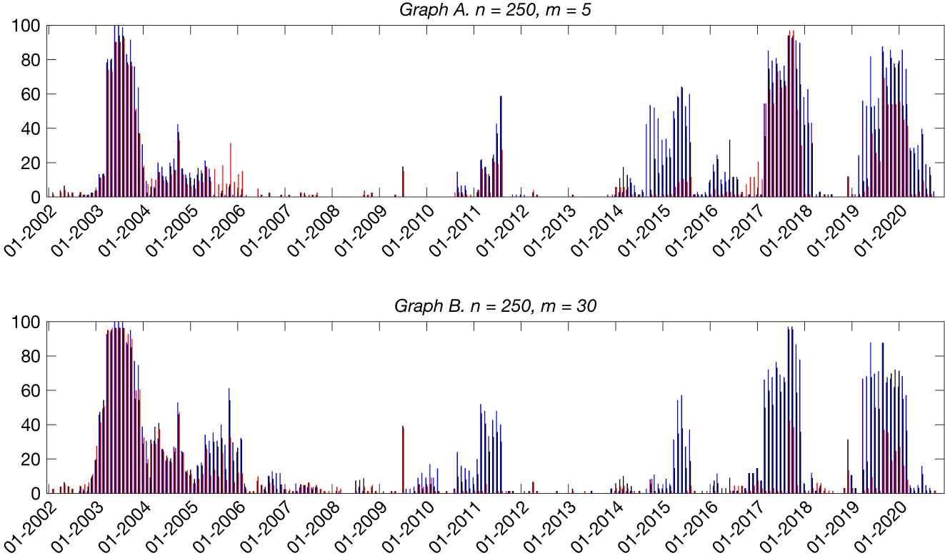
Figure 1 plots on a monthly basis the percentage of institutions with inadequate systemic risk forecasts detected by the $ Q $ backtest (depicted in blue), the $ {Q}_r $ backtest (depicted in black), and the $ {S}_r $ backtest (depicted in red). We observe that compared with $ {S}_r $ both the new backtests have higher detection frequencies over inadequate systemic risk forecasts as the blue and black bars dominate their red counterparts on many occasions. This finding holds for both $ m $ . We also observe several sizeable clusters in the plot, which we highlight and discuss in the following because these clusters imply that the systemic risk forecasts of many major institutions are inaccurate and unreliable.

Figure 1Empirical Rejection Rates

Figure 1 plots on a monthly basis the percentage of institutions with inadequate systemic risk forecasts detected using the $ Q $ backtest (depicted in blue), the $ {Q}_r $ backtest (depicted in black), and the $ {S}_r $ backtest (depicted in red). The out-sample size is denoted by $ n $ . Backtesting significance level is 5% with Bonferroni correction applied for every monthly analysis. The Bartlett kernel is used for $ Q $ and $ {Q}_r $ with kernel parameter $ m $ .

Figure 1 Long description

The figure consists of two vertically stacked panels, Graph A and Graph B. Both panels share a horizontal X-axis representing time from January 2002 to January 2020 and a vertical Y-axis representing the percentage of institutions from 0 to 100. Each month contains three colored bars: blue, black, and red.

* Graph A (n = 250, m = 5): Shows high rejection rates peaking near 100 percent between 2003 and 2004. Rates remain low until a moderate spike in 2011, followed by significant volatility and high peaks between 2014 and 2016, and again from 2017 to 2018. A final large cluster of high rejection rates appears in 2019.

* Graph B (n = 250, m = 30): Displays a similar temporal pattern to Graph A but with slightly different magnitudes in the peaks. The 2003 to 2004 peak is broader and more sustained. The spikes in 2011, 2015, and 2017 to 2018 are prominent, with the blue bars often reaching higher than the red or black bars during these periods of systemic risk forecast inadequacy.

In both graphs, the periods of 2006 to 2010 and 2012 to 2014 show near-zero rejection rates across all three backtests.

In the cluster between January 2003 and January 2004, the performance of all backtests is rather similar. More precisely, the monthly average rejection frequencies by $ Q $ , $ {Q}_r $ , and $ {S}_r $ are, respectively, 64%, 56%, and 54%, at $ m=5 $ . When $ m=30 $ , the average rejection rates are 75%, 70%, and 72% for $ Q $ , $ {Q}_r $ , and $ {S}_r $ , respectively. In this cluster, we observe for all three backtests an increase in rejection frequencies as $ m $ increases. This is consistent with our expectation that by increasing the $ m $ parameter, the testing scope of a backtest increases, which in turn may lead to the backtest detecting a more diverse forms of systemic risk inadequacy. Economically, the tall 2003–2004 cluster suggests that the risk forecasts of many institutions for the period 2004–2005 were highly inadequate. This reflects the 2004–2005 credit deterioration of the U.S. market, which at its height saw the credit deterioration of several major U.S. entities such as General Motors to the junk status. Besides, the finding could also be attributed to the fact that the DCC-GARCH specification is simply not a suitable model for systemic risk as far as this period is concerned. In practice, risk managers should consider revising the model or using alternative specifications.

In the cluster between January 2004 and January 2006, the monthly average rejection frequencies by $ Q $ , $ {Q}_r $ , and $ {S}_r $ are, respectively, 12%, 10%, and 13%, at $ m=5 $ . When $ m=30 $ , the rejection rates are 27%, 26%, and 20% for $ Q $ , $ {Q}_r $ , and $ {S}_r $ , respectively. Similar to the previous cluster, we observe an increase in rejection frequencies across all backtests when $ m $ is large. When $ m=5 $ , $ {S}_r $ has slightly better performance over $ Q $ and $ {Q}_r $ , which reverses when $ m=30 $ . The reason as to why the detection rate of $ {S}_r $ does not catch up with our backtests is likely due to it losing some power when checking a larger scope, a phenomenon too observed in our simulation study. By contrast, the rejection rates of the new backtests increase and outperform $ {S}_r $ . This highlights that the empirical alternatives captured with a large $ m $ could offset the potential loss in power when the backtest is properly weighted according to empirical stylized facts. We obtain similar conclusions for the cluster between January 2011 and July 2011.

We now discuss the remaining major clusters of model inadequacy, i.e., the cluster between July 2014 and July 2015, the 2017 cluster, and the cluster beyond January 2019. The precise monthly average rejection frequencies by ( $ Q $ , $ {Q}_r $ , $ {S}_r $ ) in the July 2014–July 2015 cluster are (40%, 24%, 3%) at $ m=5 $ , and (16%, 9%, 1%) at $ m=30 $ . In the 2017 cluster, the rejection frequencies by ( $ Q $ , $ {Q}_r $ , $ {S}_r $ ) are (68%, 59%, 52%) at $ m=5 $ , and (62%, 51%, 8%) at $ m=30 $ . The tall 2017 cluster suggests that the DCC-GARCH specification may not be a suitable model to forecast systemic risk for 2018, which could be due to the fact that this period witnessed several major international political events such as the U.S.–China trade war and the U.K.’s Brexit. In the cluster beyond January 2019, the rejection frequencies by ( $ Q $ , $ {Q}_r $ , $ {S}_r $ ) are (44%, 32%, 20%) at $ m=5 $ , and (37%, 29%, 8%) at $ m=30 $ . Given that the cluster beyond January 2019 coincides with the run-up to the pandemic-induced market crashes, we highlight the nontrivial under detection of $ {S}_r $ compared with the new backtests. In particular, $ {S}_r $ under detects 24% (12%) compared with $ Q $ ( $ {Q}_r $ ) at $ m=5 $ , and 29% (21%) compared with $ Q $ ( $ {Q}_r $ ) at $ m=30 $ . The prominence of the new backtests over $ {S}_r $ holds in the other two clusters regardless of $ m $ . Although all three backtests suffer some power reduction in $ m $ , it is minimal for the new backtests. This further highlights the optimality of our backtests in the tradeoff between losing detection power and detecting a wider alternatives as the testing scope increases.

To see the economic implications brought by the new backtests on a greater scale, we note that in any given month over the full examination period, we backtest an average of 74 financial institutions. We further note the monthly average rejection rates by ( $ Q $ , $ {Q}_r $ , $ {S}_r $ ) over the full examination period are (18%, 15%, 11%) at $ m=5 $ , and (18%, 16%, 9%) at $ m=30 $ . Compared with $ Q $ , $ {S}_r $ under detects $ 7\%\hskip0.3em \mathrm{per}\hskip0.3em \mathrm{month}\times 228\hskip0.3em \mathrm{month}\mathrm{s}\times 74\hskip0.3em \mathrm{institutions}=1181 $ cases over the course of our empirical study when $ m=5 $ . When $ m=30 $ , $ {S}_r $ under rejects 1518 (1181) cases compared with $ Q $ ( $ {Q}_r $ ). 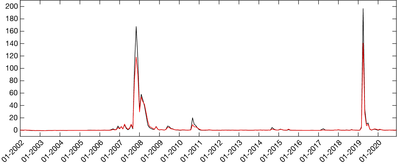We note from these numbers that the improvement of our backtests over $ {S}_r $ is of considerable economic significance, since, if the new backtests are used instead of $ {S}_r $ , a larger scale of inadequate systemic risk forecasts would have been detected among major financial institutions. These additional cases could play a critical role in prompting regulatory attention, which could call for a full-scale revision of existing systemic risk modeling in the wider economy, which in turn would improve financial stability.

Although the average findings may suggest $ Q $ regularly outperforms $ {Q}_r $ , we highlight that in some instances such as the January 2013–July 2013 period, $ {Q}_r $ has detected alternatives not captured by $ Q $ . This is in line with our simulation findings. The complementary performance of $ {Q}_r $ and $ Q $ can be attributed to them generally not capturing the same dynamics about systemic risk inaccuracy, since the former is a whitened test, whereas the latter is not. Thus, when examining the overall health of the financial system in practice, regulators could apply the formula $ \max \left(Q,{Q}_r\right) $ to detect as many indications about large-scale measure inadequacies of systemic risk as possible. This provides a “better-safe-than-sorry” approach which is recently advocated by the European Central Bank (see, e.g., Rehn (Reference Rehn2020), Enria (Reference Enria2022)).

One could argue that the empirical performance of the new backtests is only evident for a relatively small $ n $ , and that the performance of all backtests would be very comparable when $ n $ increases. To examine the sensitivity of our main findings, we repeat the backtesting analysis with a larger $ n=500 $ , and we plot the results in Figure 2. Due to the more demanding out-sample size, the time dimension of Figure 2 naturally reduces slightly compared with that of Figure 1. By the same reasoning, the average number of institutions qualified for examination reduces to 73. Compared with Figure 1, we observe an increase in rejection frequencies across all backtests. This is in line with Theorem 2 and Proposition 2 that the power of our backtests is expected to increase in $ n $ . We also observe that the overall rejection pattern for all backtests is similar to that in Figure 1, with the new backtests continue to outperform existing backtest. More precisely, the monthly average rejection rates over the full sample by ( $ Q $ , $ {Q}_r $ , $ {S}_r $ ) are (29%, 24%, 17%) at $ m=5 $ , and (30%, 26%, 13%) at $ m=30 $ . The economic implications offered by the new backtests are now more evident, as for instance, $ {S}_r $ under rejects 2,681 (2,050) cases compared with $ Q $ ( $ {Q}_r $ ) at $ m=30 $ . Unlike $ {S}_r $ , we note the rejection rates of $ Q $ and $ {Q}_r $ are similar across $ m $ , which highlights once again the optimality of our backtests as they give optimal tradeoff in $ m $ .

Figure 2Empirical Rejection Rates

Figure 2 plots on a monthly basis the percentage of institutions with inadequate systemic risk forecasts detected using the $ Q $ backtest (depicted in blue), the $ {Q}_r $ backtest (depicted in black), and the $ {S}_r $ backtest (depicted in red). The out-sample size is denoted by $ n $ . Backtesting significance level is 5% with Bonferroni correction applied for every monthly analysis. The Bartlett kernel is used for $ Q $ and $ {Q}_r $ with kernel parameter $ m $ .

Figure 2 Long description

The image consists of two vertically stacked bar charts, labeled Graph A and Graph B. Both charts share the same axes. The y-axis represents the percentage of institutions with inadequate systemic risk forecasts, ranging from 0 to 100. The x-axis represents time in monthly increments from January 2002 to January 2019. Each month contains three colored bars: blue for the J C B R I C Q backtest, black for the J C B 7 U X 1 f c i backtest, and red for the J C B 7 U 3 1 f c i backtest.

* Graph A (n = 500, m = 5): Shows high rejection rates (near 100 percent) between 2003 and 2004 across all backtests. Rates remain low from 2005 to 2009, followed by a moderate increase in blue and black bars around 2011. From 2014 to 2019, there is a significant upward trend, with blue bars frequently reaching 80 percent and red bars showing a secondary peak around 2017.

* Graph B (n = 500, m = 30): Displays a similar overall profile to Graph A but with higher volatility in the blue bars during the 2005 to 2008 period. The peak in 2003 to 2004 remains at 100 percent. The late-period trend (2016 to 2019) shows blue bars dominating with values between 60 and 80 percent, while red bars remain significantly lower than in Graph A during the same period.

To ensure that the empirical performance of the new backtests is not driven by a specific choice of kernel function, we repeat every backtesting analysis using the QS kernel, which, unlike the BAR kernel, belongs to the class of kernel with unbounded support. Figure 3 plots the analysis results for every empirical setting considered thus far. The results suggest that our main findings are highly robust as the prominence of $ Q $ and $ {Q}_r $ over existing backtest remains highly evident. This highlights, as with our simulation evidence, that the choice of kernel does not have a strong impact over the performance of our backtests so long as the kernel function is downward weighting.

Figure 3Empirical Rejection Rates

Figure 3 plots on a monthly basis the percentage of institutions with inadequate systemic risk forecasts detected using the $ Q $ backtest (depicted in blue), the $ {Q}_r $ backtest (depicted in black), and the $ {S}_r $ backtest (depicted in red). The out-sample size is denoted by $ n $ . Backtesting significance level is 5% with Bonferroni correction applied for every monthly analysis. The Quadratic-Spectral kernel is used for $ Q $ and $ {Q}_r $ with kernel parameter $ m $ .

Figure 3 Long description

A multi-panel figure consisting of four vertically stacked bar charts labeled Graph A through Graph D.

* Common Axes: The vertical y-axis represents the percentage of institutions with inadequate systemic risk forecasts, ranging from 0 to 100. The horizontal x-axis represents time in monthly increments from January 2002 to January 2020.

* Data Series: Each graph contains three overlapping bar series. Blue bars represent the J C B R I C Q backtest. Black bars represent the J C B 7 U X 1 f r i backtest. Red bars represent the J C B 7 U 3 1 f r i backtest.

* Panel A (n = 250, m = 5): Shows high rejection rates around 2003 to 2004, reaching near 100 percent. Smaller peaks occur around 2005, 2011, 2015, and a significant sustained peak from 2017 to 2018.

* Panel B (n = 250, m = 30): Displays a similar temporal pattern to Graph A but with slightly smoothed or lower peaks in the 2010 to 2015 period.

* Panel C (n = 500, m = 5): Shows a very high, dense rejection period between 2003 and 2004. Rejection rates are notably higher and more sustained in the blue series from 2014 through 2019 compared to the n = 250 panels.

* Panel D (n = 500, m = 30): Similar to Graph C, showing the highest density of rejections in the early 2000s and late 2010s, with the blue series consistently showing higher rejection rates than the black or red series in the latter half of the timeline.

Finally, we perform a robustness analysis by whitening $ {\hat{\rho}}_n(j) $ up to the same order as the kernel parameter, i.e., we have $ {\hat{\rho}}_n(j) $ being whitened up to order $ m $ , which we denote by $ {\hat{\rho}}_{nrm}(j) $ , $ j=1,\dots, m $ . Such partial whitening does not affect the computation of truncated whitened backtests such as $ {S}_r $ and $ {Q}_r $ with a truncated kernel. In particular, $ {\hat{\rho}}_{nrm}(j) $ is the $ j $ th element of the vector $ {\hat{\varDelta}}_m^{-1/2}{\hat{\boldsymbol{\rho}}}_n^{(m)} $ , where $ {\hat{\boldsymbol{\rho}}}_n^{(m)} $ collects $ {\left\{{\hat{\rho}}_n(j)\right\}}_{j=1}^m $ , and $ {\hat{\varDelta}}_m $ is a $ m\times m $ matrix with the same $ \left(i,j\right) $ th element as that in $ \hat{\varDelta} $ . The Box–Pierce-type statistic based on $ {\hat{\rho}}_{nrm}(j) $ is given by $ {S}_r=n{\sum}_{j=1}^m{\hat{\rho}}_{nrm}^2(j) $ . For proper comparison, we also use $ {\hat{\rho}}_{nrm} $ in our whitened backtest $ {Q}_r $ with the Bartlett kernel. We plot the results in Figure 4, and we can see that the rejection patterns are very similar to those in Figures 1 and 2. The improvement brought by the new backtests remains highly evident and robust.

Figure 4Empirical Rejection Rates

Figure 4 plots on a monthly basis the percentage of institutions with inadequate systemic risk forecasts detected using the $ Q $ backtest (depicted in blue), the $ {Q}_r $ backtest (depicted in black), and the $ {S}_r $ backtest (depicted in red). The out-sample size is denoted by $ n $ . Backtesting significance level is 5% with Bonferroni correction applied for every monthly analysis. The Bartlett kernel is used for $ Q $ and $ {Q}_r $ with kernel parameter $ m $ . $ {Q}_r $ and $ {S}_r $ are computed using $ {\hat{\rho}}_{nrm}(j) $ .

Figure 4 Long description

The multi-panel figure consists of four bar charts labeled Graph A through Graph D. Each chart shares a common y-axis representing the percentage of institutions from 0 to 100 and an x-axis representing time from January 2002 to January 2020. Each month contains three colored bars: blue for J C B R I C Q, black for J C B 7 U X 1 f c i k, and red for J C B 7 U 3 1 f c i k.

* Graph A (n = 250, m = 5): Shows high rejection rates (near 100 percent) around 2003 to 2004 and 2017 to 2018. Rejection rates are generally lower between 2006 and 2014.

* Graph B (n = 250, m = 30): Displays similar peaks to Graph A but with slightly more volatility in the black and blue bars during the 2015 to 2020 period.

* Graph C (n = 500, m = 5): Shows a sustained high rejection rate for the blue and black tests from 2016 onwards, while the red test remains significantly lower in that same period.

* Graph D (n = 500, m = 30): Exhibits the most dense rejection activity, with the blue and black bars frequently exceeding 60 percent from 2016 to 2020, while the red bars show minimal activity in the latter half of the timeline.

Across all graphs, a major spike in rejection rates for all three tests occurs between 2003 and 2004, corresponding to a period of high systemic risk detection.

C. Summary and Regulatory Implications

In summary, using real-world data generated by the major U.S. financial institutions, we find that, compared with existing approach, the new backtests $ Q $ and $ {Q}_r $ offer better empirical power as they reveal thousands more cases of systemic risk inadequacies. Such improvement is also of considerable economic significance. Our findings remain robust under a series of sensitivity analyses including using alternative kernel parameters, alternative sample sizes, and alternative kernel classes. Because of their complementary features, $ Q $ and $ {Q}_r $ can be applied together to detect as many indications about large-scale measure inadequacies of systemic risk as possible. This provides a useful “better-safe-than-sorry” approach for financial supervisors and regulators.

We acknowledge that despite being estimated from an inadequate risk model, systemic risk measures may still be useful in, e.g., ranking financial institutions by their systemic relevance. This can be attributed to ranking operations being impartial to effects that are uniform across all institutions such as inaccuracy from using the same (inadequate) risk model. Using the same risk model for a group of institutions is also fairly standard in the academic literature (see, e.g., Brownlees and Engle (Reference Brownlees and Engle2017), Banulescu-Radu et al. (Reference Banulescu-Radu, Hurlin, Leymarie and Scaillet2021)). In reality, however, each financial institution usually has its own proprietary risk model, which is regularly tested for accuracy and is subject to ongoing refinement. In this aspect, $ Q $ and $ {Q}_r $ serve as new statistical tools for checking, with better power, whether a risk model can be further improved to produce more accurate systemic risk estimates. With more accurate risk estimates across all financial institutions, financial stability will improve as a collective result.