


%20--%3e%3c!DOCTYPE%20svg%20PUBLIC%20'-//W3C//DTD%20SVG%201.0//EN'%20'http://www.w3.org/TR/2001/REC-SVG-20010904/DTD/svg10.dtd'%3e%3csvg%20version='1.0'%20id='Layer_1'%20xmlns='http://www.w3.org/2000/svg'%20xmlns:xlink='http://www.w3.org/1999/xlink'%20x='0px'%20y='0px'%20width='64px'%20height='64px'%20viewBox='5.5%20-3.5%2064%2064'%20enable-background='new%205.5%20-3.5%2064%2064'%20xml:space='preserve'%3e%3cg%3e%3ccircle%20fill='%23FFFFFF'%20fill-opacity='0'%20cx='37.785'%20cy='28.501'%20r='28.836'/%3e%3cpath%20fill='%23595959'%20d='M37.441-3.5c8.951,0,16.572,3.125,22.857,9.372c3.008,3.009,5.295,6.448,6.857,10.314%20c1.561,3.867,2.344,7.971,2.344,12.314c0,4.381-0.773,8.486-2.314,12.313c-1.543,3.828-3.82,7.21-6.828,10.143%20c-3.123,3.085-6.666,5.448-10.629,7.086c-3.961,1.638-8.057,2.457-12.285,2.457s-8.276-0.808-12.143-2.429%20c-3.866-1.618-7.333-3.961-10.4-7.027c-3.067-3.066-5.4-6.524-7-10.372S5.5,32.767,5.5,28.5c0-4.229,0.809-8.295,2.428-12.2%20c1.619-3.905,3.972-7.4,7.057-10.486C21.08-0.394,28.565-3.5,37.441-3.5z%20M37.557,2.272c-7.314,0-13.467,2.553-18.458,7.657%20c-2.515,2.553-4.448,5.419-5.8,8.6c-1.354,3.181-2.029,6.505-2.029,9.972c0,3.429,0.675,6.734,2.029,9.913%20c1.353,3.183,3.285,6.021,5.8,8.516c2.514,2.496,5.351,4.399,8.515,5.715c3.161,1.314,6.476,1.971,9.943,1.971%20c3.428,0,6.75-0.665,9.973-1.999c3.219-1.335,6.121-3.257,8.713-5.771c4.99-4.876,7.484-10.99,7.484-18.344%20c0-3.543-0.648-6.895-1.943-10.057c-1.293-3.162-3.18-5.98-5.654-8.458C50.984,4.844,44.795,2.272,37.557,2.272z%20M37.156,23.187%20l-4.287,2.229c-0.458-0.951-1.019-1.619-1.685-2c-0.667-0.38-1.286-0.571-1.858-0.571c-2.856,0-4.286,1.885-4.286,5.657%20c0,1.714,0.362,3.084,1.085,4.113c0.724,1.029,1.791,1.544,3.201,1.544c1.867,0,3.181-0.915,3.944-2.743l3.942,2%20c-0.838,1.563-2,2.791-3.486,3.686c-1.484,0.896-3.123,1.343-4.914,1.343c-2.857,0-5.163-0.875-6.915-2.629%20c-1.752-1.752-2.628-4.19-2.628-7.313c0-3.048,0.886-5.466,2.657-7.257c1.771-1.79,4.009-2.686,6.715-2.686%20C32.604,18.558,35.441,20.101,37.156,23.187z%20M55.613,23.187l-4.229,2.229c-0.457-0.951-1.02-1.619-1.686-2%20c-0.668-0.38-1.307-0.571-1.914-0.571c-2.857,0-4.287,1.885-4.287,5.657c0,1.714,0.363,3.084,1.086,4.113%20c0.723,1.029,1.789,1.544,3.201,1.544c1.865,0,3.18-0.915,3.941-2.743l4,2c-0.875,1.563-2.057,2.791-3.541,3.686%20c-1.486,0.896-3.105,1.343-4.857,1.343c-2.896,0-5.209-0.875-6.941-2.629c-1.736-1.752-2.602-4.19-2.602-7.313%20c0-3.048,0.885-5.466,2.658-7.257c1.77-1.79,4.008-2.686,6.713-2.686C51.117,18.558,53.938,20.101,55.613,23.187z'/%3e%3c/g%3e%3c/svg%3e)
%20--%3e%3c!DOCTYPE%20svg%20PUBLIC%20'-//W3C//DTD%20SVG%201.0//EN'%20'http://www.w3.org/TR/2001/REC-SVG-20010904/DTD/svg10.dtd'%3e%3csvg%20version='1.0'%20id='Layer_1'%20xmlns='http://www.w3.org/2000/svg'%20xmlns:xlink='http://www.w3.org/1999/xlink'%20x='0px'%20y='0px'%20width='64px'%20height='64px'%20viewBox='5.5%20-3.5%2064%2064'%20enable-background='new%205.5%20-3.5%2064%2064'%20xml:space='preserve'%3e%3cg%3e%3ccircle%20fill='%23FFFFFF'%20fill-opacity='0'%20cx='37.637'%20cy='28.806'%20r='28.276'/%3e%3cg%3e%3cpath%20fill='%23595959'%20d='M37.443-3.5c8.988,0,16.57,3.085,22.742,9.257C66.393,11.967,69.5,19.548,69.5,28.5c0,8.991-3.049,16.476-9.145,22.456%20C53.879,57.319,46.242,60.5,37.443,60.5c-8.649,0-16.153-3.144-22.514-9.43C8.644,44.784,5.5,37.262,5.5,28.5%20c0-8.761,3.144-16.342,9.429-22.742C21.101-0.415,28.604-3.5,37.443-3.5z%20M37.557,2.272c-7.276,0-13.428,2.553-18.457,7.657%20c-5.22,5.334-7.829,11.525-7.829,18.572c0,7.086,2.59,13.22,7.77,18.398c5.181,5.182,11.352,7.771,18.514,7.771%20c7.123,0,13.334-2.607,18.629-7.828c5.029-4.838,7.543-10.952,7.543-18.343c0-7.276-2.553-13.465-7.656-18.571%20C50.967,4.824,44.795,2.272,37.557,2.272z%20M46.129,20.557v13.085h-3.656v15.542h-9.944V33.643h-3.656V20.557%20c0-0.572,0.2-1.057,0.599-1.457c0.401-0.399,0.887-0.6,1.457-0.6h13.144c0.533,0,1.01,0.2,1.428,0.6%20C45.918,19.5,46.129,19.986,46.129,20.557z%20M33.042,12.329c0-3.008,1.485-4.514,4.458-4.514s4.457,1.504,4.457,4.514%20c0,2.971-1.486,4.457-4.457,4.457S33.042,15.3,33.042,12.329z'/%3e%3c/g%3e%3c/g%3e%3c/svg%3e)
I. Introduction
Corporate diversification, with its potential impact on firm value and risk, has attracted the interest of academics and management practitioners alike.Footnote 1 A key strand of the corporate diversification literature investigates its impact on debt capacity. In particular, Galai and Masulis (Reference Galai and Masulis1976) and Lewellen (Reference Lewellen1971) claim that diversified firms can exploit the coinsurance effect across their divisions to increase their leverage, but empirical evidence in this respect is mixed (Berger and Ofek (Reference Berger and Ofek1995), Mansi and Reeb (Reference Mansi and Reeb2002)). However, leverage is only one of the channels through which corporate diversification might affect firm value via the coinsurance effect.
In this article, we are the first to investigate both theoretically and empirically the interplay between corporate diversification and debt maturity choices and their effect on firm value. Recent contributions have studied the role of debt maturity choices for investment incentives, rollover risk, and the debt overhang problem (see, e.g., Myers (Reference Myers1977), Diamond (Reference Diamond1991), Barclay and Smith (Reference Barclay and Smith1995), Cheng and Milbradt (Reference Cheng and Milbradt2012), Chen, Xu, and Yang (Reference Chen, Xu and Yang2012), Diamond and He (Reference Diamond and He2014), Gopalan, Song, and Yerramilli (Reference Gopalan, Song and Yerramilli2014), and Dangl and Zechner (2021)).Footnote 2 However, the literature has, insofar, neglected the role of corporate diversification in shaping debt maturity choices. We argue that corporate diversification allows companies to have a longer average debt maturity than stand-alone firms by alleviating the debt-overhang problem.
Our theoretical contribution consists of a simple 3-period discrete-time model and a continuous-time model based on a basket option pricing approach. The 3-period model extends Diamond and He’s (Reference Diamond and He2014) numerical example of how debt maturity can affect debt overhang to a multi-division setting.Footnote 3 Although corporate diversification reduces the conditional variance of the multi-division firm’s future payoffs (i.e., the coinsurance effect), it does not affect the value of an all-equity firm because it does not alter the expected payoffs, consistent with Mansi and Reeb’s (Reference Mansi and Reeb2002) findings. When we introduce the possibility for firms to raise debt, the coinsurance effect allows a multi-division firm to have a lower book value of debt than a comparable stand-alone firm. The lower book leverage reduces the default risk of the multi-division firm and, therefore, mitigates debt overhang in both the short and long terms. Once we allow for higher noninterest debt expenses for short-term debt (see, e.g., Acharya, Gale, and Yorulmazer (Reference Acharya, Gale and Yorulmazer2011)),Footnote 4 our model predicts that multi-division (stand-alone) firms are more likely to issue long-term (short-term) debt.
The idea that short-term debt improves investment incentives (Myers (Reference Myers1977)) originates from the Black–Scholes–Merton model, in which equity is analogous to a European call option with a strike price equal to the face value of the debt due at maturity (Diamond and He (Reference Diamond and He2014)). To further study the corporate diversification’s effect on debt maturity, we generalize our 3-period model using a Black–Scholes–Merton approach, considering the multi-division firm’s equity value as a European basket call option. We use Ju’s (Reference Ju2002) approach as an efficient closed-form approximation of the basket call option to price the equity value of the multi-division firm. This model allows us to conduct more flexible counterfactual analyses. The basket-option framework leads to the same conclusion as the 3-period model: the optimal debt maturity (i.e., the one that maximizes investment incentives) is shorter for stand-alone firms than for multi-division firms. This theoretical prediction, for which we find strong empirical support, has important implications for the diversification discount/premium measure: the presence of the coinsurance effect might lead multi-division firms to have longer debt maturity compared with stand-alone firms.Footnote 5 Longer-term debt makes the market value of equity of multi-division firms higher than that of comparable stand-alone firms. Conventional measures of excess value could be misleading because they neglect the endogenous nature of debt maturity preferences. Our model predicts that the excess value measure introduced by Berger and Ofek (Reference Berger and Ofek1995) and Mansi and Reeb (Reference Mansi and Reeb2002), which is not adjusted for debt maturity, increases with debt maturity.Footnote 6
We test the empirical predictions of our models and their assumptions on a sample of stand-alone and multi-division firms. Our main findings are as follows: First, our regression results confirm a positive association between corporate diversification and debt maturity. Multi-division firms have a debt maturity at least 1 year longer than stand-alone firms, with a median stand-alone firm increasing debt maturity by 25% through diversification. Compared with other determinants of debt maturity, corporate diversification has a larger incremental explanatory power than the debt-to-equity ratio, net income, and capital expenditures. The only variable with a larger incremental explanatory power than corporate diversification is size (market value of equity), but the positive effect of corporate diversification on debt maturity remains positive across three size-based subsamples. Thus, the positive impact of corporate diversification on debt maturity is distinct from the effect of firm size. However, the magnitude of the impact becomes smaller and less statistically significant for larger firms, plausibly because smaller firms have better growth options.
Second, we provide evidence that the positive effect of corporate diversification on debt maturity is stronger for firms with debt overhang. This finding is important because it supports the view that corporate diversification leads to longer debt maturities by mitigating the debt overhang problem, which is consistent with our model. These results are robust to using different proxies for debt overhang, including the one introduced by Alanis et al. (Reference Alanis, Chava and Kumar2018), which uses a model introduced by Chava and Jarrow (Reference Chava and Jarrow2004) to estimate the probability of default.
Third, we find a positive and statistically significant relationship between the excess value (Berger and Ofek (Reference Berger and Ofek1995), Mansi and Reeb (Reference Mansi and Reeb2002)) and debt maturity, consistent with the predictions of our basket-option model: a 1-standard-deviation increase in the natural logarithm of debt maturity leads to a 1.6% increase in the excess value.Footnote 7
In our empirical exercise, we also provide evidence supporting our models’ assumptions. Specifically, we find that a 1-standard-deviation decrease in the logarithm of debt maturity results in a 0.23-standard-deviation increase in the cost of debt, equivalent to a 4% increase. This finding supports the assumption of a negative correlation between debt maturity and the cost of debt in our theoretical models. Moreover, we provide evidence of an economically negligible difference in the leverage of the stand-alone and multi-division firms (only 40 BPS or 0.4%). This result is consistent with the setup of our basket-option model, where we require that the face value of debt for the stand-alone and multi-division firms be the same.
The central contribution of our article lies in bridging a gap between two strands of literature: one on the determinants of debt maturity and the other on corporate diversification. Debt maturity affects shareholders’ investment incentives (Myers (Reference Myers1977)), and short-term debt mitigates debt overhang. Diamond and He’s (Reference Diamond and He2014) theory offers further nuance to our understanding of the relationship between debt maturity and debt overhang. Our article contributes to the debt maturity literature by offering an analytical framework quantifying corporate diversification’s effect on lengthening debt maturity for multi-division firms due to reduced debt overhang.
From a purely theoretical perspective, there could be both costs and benefits associated with corporate diversification. From an empirical perspective, there is still a debate as to whether corporate diversification has any impact on firm value (e.g., Lang and Stulz (Reference Lang and Stulz1994), Berger and Ofek (Reference Berger and Ofek1995), Lamont and Polk (Reference Lamont and Polk2002), Rajan, Servaes, and Zingales (Reference Rajan, Servaes and Zingales2000), Denis, Denis, and Sarin (Reference Denis, Denis and Sarin1997), Levinthal and Wu (Reference Levinthal and Wu2010), and Hund et al. (Reference Hund, Monk and Tice2024)). The diversification discount could be related to endogeneity due to self-selection bias (Campa and Kedia (Reference Campa and Kedia2002), Lamont and Polk (Reference Lamont and Polk2002), Chevalier (Reference Chevalier2004), Villalonga (Reference Villalonga2004b), and Xiao and Xu (Reference Xiao and Xu2019)) or measurement error (Whited (Reference Whited2001)). After adjusting for these factors, the diversification discount tends to disappear. Moreover, focusing on establishment-level diversification, instead of business segments provided by Compustat, Villalonga (Reference Villalonga2004a) finds evidence of a diversification premium.
While most of the literature on corporate diversification tends to be empirical, recent contributions develop theoretical models allowing for endogeneity of the choice to become a diversified firm. For example, Bakke and Gu (Reference Bakke and Gu2017) focus on the relationship between corporate diversification and cash holdings. They estimate a structural model where the switch from stand-alone to multi-division firms is endogenously determined because diversifying firms tend to be larger and have better growth opportunities. Dai, Giroud, Jiang, and Wang (Reference Dai, Giroud, Jiang and Wang2024) highlight that resource allocation within the firm considers not only divisions’ productivity but also their risk, and firms may opt to spin off productive divisions voluntarily to enhance liquidity. Their results echo the mixed findings from the empirical literature and emphasize the importance of accounting for the endogenous formation of conglomerates. We contribute to this literature by providing insights into a new channel, debt maturity. Our models show that the debt maturity choices are endogenous to divisional structure. When estimating the excess value, such endogeneity cannot be resolved by matching diversified firms with a control sample of stand-alone firms. Our theoretical and empirical results suggest that the conventional excess value measure could be misleading because of the endogenous nature of debt maturity in association with corporate diversification.
II. Three-Period Model
We first study a simple 3-period model extending Diamond and He’s (Reference Diamond and He2014) 3-period numerical example of a stand-alone firm to a multi-division setting. For easy comparison, we model two firms with assets-in-place of identical size: one,
 $ S $
, with a single division and the other,
 $ M $
, with two divisions. Each of the assets-in-place of
 $ M $
,
 $ {F}_m $
, is one-half of the assets-in-place of
 $ S $
,
 $ {F}_s $
.
 $ S $
’s (each of
 $ M $
’s) assets-in-place will generate three possible cash flows at
 $ t=2 $
as {24, 12, 0} ({12, 6, 0}), with probability
 $ \frac{1}{3} $
of each scenario, conditional on the information at
 $ t=0 $
. The same applies to the assets-in-place of the two divisions of
 $ M $
. The distributions of
 $ {F}_m $
’s two assets-in-place cash flows are independent of each other. There are no cash flows in other periods. The discount rate is 0.
For simplicity, we assume firm value maximization, given a firm’s divisional structure (Myers (Reference Myers1977), Damodaran (Reference Damodaran2014), and Diamond and He (Reference Diamond and He2014)).Footnote 8
A. Information Structure and Payoffs
For all three assets-in-place, there are two states: a good state and a bad state. The state of the economy is revealed at
 $ t=1 $
. We use notations
 $ G $
(good) and
 $ B $
(bad) to represent the two states of the assets-in-place for the stand-alone firm (
 $ {F}_s $
). For the multi-division firm, we denote the states for the assets-in-place of the first division (
 $ {F}_m(1) $
) as
 $ G1 $
and
 $ B1 $
, and for the assets-in-place of the second division (
 $ {F}_m(2) $
) as
 $ G2 $
and
 $ B2 $
. The probability of each state is
 $ \frac{1}{2} $
, and the outcomes are independent across all assets-in-place. For any given asset-in-place, the conditional probabilities of the cash flow at
 $ t=2 $
are as follows: If the state at
 $ t=1 $
is good (bad), the probabilities are
 $ \frac{1}{2} $
,
 $ \frac{1}{3} $
,
 $ \frac{1}{6} $
(
 $ \frac{1}{6} $
,
 $ \frac{1}{3} $
,
 $ \frac{1}{2} $
). The conditional distributions of
 $ {F}_s $
at
 $ t=2 $
, based on the information from
 $ t=0 $
and
 $ t=1 $
, areFootnote 9
 $$ \underset{t=0}{\underbrace{{\left.{F}_s\right|}_{t=0}=\left\{\begin{array}{cc}24,& \mathrm{with}\hskip0.33em \mathrm{prob}=1/3,\\ {}12,& \mathrm{with}\hskip0.33em \mathrm{prob}=1/3,\\ {}0,& \mathrm{with}\hskip0.33em \mathrm{prob}=1/3,\end{array}\right.}} $$
 $$ \underset{t=1}{\underbrace{{\left.{F}_s\right|}_{\operatorname{G},t=1}=\left\{\begin{array}{cc}24,& \mathrm{with}\ \mathrm{prob}=1/2,\\ {}12,& \mathrm{with}\ \mathrm{prob}=1/3,\\ {}0,& \mathrm{with}\ \mathrm{prob}=1/6,\end{array}\right.\hskip0.24em {\left.{F}_s\right|}_{\operatorname{B},t=1}=\left\{\begin{array}{cc}24,& \mathrm{with}\ \mathrm{prob}=1/6,\\ {}12,& \mathrm{with}\ \mathrm{prob}=1/3,\\ {}0,& \mathrm{with}\ \mathrm{prob}=1/2,\end{array}\right.}} $$
and the conditional expectation of
 $ {F}_s $
at
 $ t=2 $
, given the information from
 $ t=1 $
, is
 $$ \unicode{x1D53C}({\left.{F}_s\right|}_{\varPi_s,t=1})=\left\{\begin{array}{cc}16,& \mathrm{with}\hskip0.33em {\Pi}_s=G,\\ {}8,& \mathrm{with}\hskip0.33em {\Pi}_s=B,\end{array}\right. $$
where
 $ {\Pi}_s $
is the state variable for
 $ {F}_s $
, which can take two realizations,
 $ G $
and
 $ B $
, with equal probability.
Since
 $ {F}_m(1) $
and
 $ {F}_m(2) $
are independent and
 $ {F}_m={F}_m(1)+{F}_m(2) $
, we obtain
 $ {F}_m $
’s conditional distribution by convolving the distributions of
 $ {F}_m(1) $
and
 $ {F}_m(2) $
:
 $$ \underset{t=0}{\underbrace{{\left.{F}_m\right|}_{t=0}=\left\{\begin{array}{cc}24,& \mathrm{with}\ \mathrm{prob}=1/9,\\ {}18,& \mathrm{with}\ \mathrm{prob}=2/9,\\ {}12,& \mathrm{with}\ \mathrm{prob}=1/3,\\ {}6,& \mathrm{with}\ \mathrm{prob}=2/9,\\ {}0,& \mathrm{with}\ \mathrm{prob}=1/9,\end{array}\right.}}\hskip1.2em \underset{t=1}{\underbrace{{\left.{F}_m\right|}_{G1G2,t=1}=\left\{\begin{array}{cc}24,& \mathrm{with}\ \mathrm{prob}=1/4,\\ {}18,& \mathrm{with}\ \mathrm{prob}=1/3,\\ {}12,& \mathrm{with}\ \mathrm{prob}=5/18,\\ {}6,& \mathrm{with}\ \mathrm{prob}=1/9,\\ {}0,& \mathrm{with}\ \mathrm{prob}=1/36,\end{array}\right.}} $$
 $$ \underset{t=1}{\underbrace{{\left.{F}_m\right|}_{B1B2,t=1}=\left\{\begin{array}{cc}24,& \mathrm{with}\ \mathrm{prob}=1/36,\\ {}18,& \mathrm{with}\ \mathrm{prob}=1/9,\\ {}12,& \mathrm{with}\ \mathrm{prob}=5/18,\\ {}6,& \mathrm{with}\ \mathrm{prob}=1/3,\\ {}0,& \mathrm{with}\ \mathrm{prob}=1/4,\end{array}\right.\hskip0.24em {\left.{F}_m\right|}_{G1B2\mathrm{or}B1G2,t=1}=\left\{\begin{array}{cc}24,& \mathrm{with}\ \mathrm{prob}=1/12,\\ {}18,& \mathrm{with}\ \mathrm{prob}=2/9,\\ {}12,& \mathrm{with}\ \mathrm{prob}=7/18,\\ {}6,& \mathrm{with}\ \mathrm{prob}=2/9,\\ {}0,& \mathrm{with}\ \mathrm{prob}=1/12,\end{array}\right.}} $$
the conditional expectation of
 $ {F}_m $
at
 $ t=2 $
, given the information at
 $ t=1 $
, is
 $$ \unicode{x1D53C}({\left.{F}_m\right|}_{\varPi_m,t=1})=\left\{\begin{array}{cc}16,& \mathrm{with}\hskip0.33em {\Pi}_m=G1G2,\\ {}12,& \mathrm{with}\hskip0.33em {\Pi}_m=G1B2\hskip0.33em \mathrm{or}\hskip0.33em B1G2,\\ {}8,& \mathrm{with}\hskip0.33em {\Pi}_m=B1B2,\end{array}\right. $$
and
 $ {F}_m $
’s state variable
 $ {\Pi}_m $
has three realizations, and its distribution is given by
 $$ {\left.{\varPi}_m\right|}_{t=0}=\left\{\begin{array}{cc}G1G2,& \mathrm{with}\ \mathrm{prob}=1/4,\\ {}G1B2\hskip0.33em \mathrm{or}\hskip0.33em B1G2,& \mathrm{with}\ \mathrm{prob}=1/2,\\ {}B1B2,& \mathrm{with}\ \mathrm{prob}=1/4.\end{array}\right. $$
The binomial tree representations of the possible paths of
 $ {F}_s $
and
 $ {F}_m $
in the 2 periods are presented in Figures 1 and 2, respectively. It is worth noting that the firm value is invariant to corporate diversification when the firm is an all-equity firm, as
 $ \unicode{x1D53C}\left({\left.{F}_s\right|}_{t=0}\right)=\unicode{x1D53C}\left({\left.{F}_m\right|}_{t=0}\right)=12 $
. This is consistent with Mansi and Reeb (Reference Mansi and Reeb2002), in that for all-equity firms, corporate diversification is unrelated to excess total firm value. However, corporate diversification does reduce the conditional standard deviation of future firm value:
 $ \mathrm{Std}\left({\left.{F}_m\right|}_{t=0}\right)=6.93<9.80=\mathrm{Std}\left({\left.{F}_s\right|}_{t=0}\right) $
. This is consistent with the coinsurance effect of corporate diversification argued by Lewellen (Reference Lewellen1971), Galai and Masulis (Reference Galai and Masulis1976), and Hann et al. (Reference Hann, Ogneva and Ozbas2013).
Figure 1 plots all possible values of stand-alone firm
 $ S $
’s assets-in-place on
 $ t=2 $
and two states
 $ \left\{G\hskip0.42em \mathrm{and}\hskip0.42em B\right\} $
on
 $ t=1 $
. The probability of each path is shown along the path. Long-term and short-term face values of debt are indicated in the figure as long and short lines with corresponding legends.

In Figure 2, Graphs A and B plot all possible values of multi-division firm
 $ M $
’s two assets-in-place
 $ {F}_m(1) $
and
 $ {F}_m(2) $
, respectively, on
 $ t=2 $
and two states
 $ \left\{G\hskip0.42em \mathrm{and}\hskip0.42em B\right\} $
on
 $ t=1 $
. The probability of each path is shown along the path. Graph C plots the same paths for the combined assets-in-place
 $ {F}_m $
for firm
 $ M $
. Long-term and short-term face values of debt are indicated in Graph C as long and short lines with corresponding legends.

B. Debt Overhang and Investment Incentives
We now introduce debt into the firm value to study the effect of corporate diversification on debt overhang and shareholders’ incentives. We follow Diamond and He (Reference Diamond and He2014) and assume that both
 $ S $
and
 $ M $
need to raise
 $ 8.25 $
at
 $ t=0 $
. The debt can be either long-term (maturing at
 $ t=2 $
) or short-term (maturing at
 $ t=1 $
). As shown in Diamond and He (Reference Diamond and He2014), given the payoffs above and the need to raise
 $ 8.25 $
, the short-term and long-term debt’s nominal values are
 $ {L}_s^{\mathrm{ST}}=8.5 $
and
 $ {L}_s^{\mathrm{LT}}=12.75 $
for
 $ S $
. Our model extension to the multi-division firm leads to
 $ {L}_m^{\mathrm{ST}}=8.33 $
and
 $ {L}_m^{\mathrm{LT}}=10.38 $
for
 $ M $
. Figures 1 and 2 illustrate the relationship between the payoffs and the nominal values of debt for
 $ S $
and
 $ M $
, respectively. The discrepancy between the nominal debt value of
 $ S $
and that of
 $ M $
arises from the reduction in default risk due to the coinsurance effect.Footnote 10 We assume that there is no cost to raise either short-term or long-term debt.Footnote 11 For simplicity, we focus on an infinitesimal investment that only weakly increases or leaves unchanged the value of each of its debt and equity claims.Footnote 12 Such investment occurs immediately after raising the debt at
 $ t=0 $
, and results in a marginal increment of the final cash flows at
 $ t=2 $
equal to
 $ \varepsilon >0 $
. The short-term (
 $ {O}_i^{\mathrm{ST}} $
) and long-term debt overhang (
 $ {O}_i^{\mathrm{LT}} $
) are
 $$ {O}_i^{\mathrm{ST}}={\unicode{x1D53C}}_0({\mathbf{1}}_{\{\unicode{x1D53C}({\operatorname{}{F}_i|}_{t=1})<{L}_i^{\mathrm{ST}}\}})\hskip0.33em \mathrm{a}\mathrm{n}\mathrm{d}\hskip0.42em {O}_i^{\mathrm{LT}}={\unicode{x1D53C}}_0({\mathbf{1}}_{\{{F}_i\ \mathrm{a}\mathrm{t}\ t=2<{L}_i^{\mathrm{LT}}\}}),\hskip0.6em \mathrm{f}\mathrm{o}\mathrm{r}\hskip0.42em i=s\hskip0.33em \mathrm{a}\mathrm{n}\mathrm{d}\hskip0.33em m, $$
where
 $ {\mathbf{1}}_{\left\{\cdot \right\}} $
is an indicator function that equals 1 when the condition in
 $ \left\{\cdot \right\} $
holds, and 0 otherwise. Combining (8) with the conditional distributions of
 $ {F}_s $
and
 $ {F}_m $
, we have
 $$ {O}_s^{\mathrm{ST}}=\frac{1}{2},\hskip1em {O}_s^{\mathrm{LT}}=\frac{2}{3},\hskip1em {O}_m^{\mathrm{ST}}=\frac{1}{4},\hskip1em \mathrm{and}\hskip1em {O}_m^{\mathrm{LT}}=\frac{1}{3}. $$
Comparing
 $ {O}_s^{\mathrm{ST}} $
with
 $ {O}_m^{\mathrm{ST}} $
and
 $ {O}_s^{\mathrm{LT}} $
with
 $ {O}_m^{\mathrm{LT}} $
shows that corporate diversification mitigates debt overhang in the short term and the long term. Moreover,
 $ {O}_m^{\mathrm{LT}}-{O}_m^{\mathrm{ST}}<{O}_s^{\mathrm{LT}}-{O}_s^{\mathrm{ST}} $
. Thus, corporate diversification reduces the difference between long-term and short-term debt overhang (the wedge).Footnote 13
Now, we describe how corporate diversification affects investment incentives. Denote the percentage investment cost by
 $ \lambda $
, and let
 $$ \left(1-\lambda \right)>{O}_i^j, $$
where
 $ i\in \left\{s,m\right\} $
and
 $ j\in \left\{ ST, LT\right\} $
. This condition implies that a firm invests only in projects with an NPV exceeding the debt overhang.
For
 $ S $
’s shareholders, the condition above is satisfied if
 $ \lambda <1/3 $
, regardless of whether the firm raises short-term or long-term debt, implying an internal rate of return (
 $ \mathrm{IRR}=\left(1-\lambda \right)/\lambda $
), larger than
 $ 200\% $
. For
 $ M $
’s shareholders, the condition becomes
 $ \lambda <2/3 $
, or equivalently
 $ \mathrm{IRR}>50\% $
. Focusing on the optimal choice for short-term debt only, the investment condition modifies to
 $ \lambda <1/2 $
(
 $ \mathrm{IRR}>100\% $
) for
 $ S $
’s shareholders and
 $ \lambda <3/4 $
(
 $ \mathrm{IRR}>33.\overline{3}\% $
) for
 $ M $
’s shareholders. Therefore, all else being equal, a multi-division firm is more likely to invest in new projects than a comparable stand-alone firm. This occurs because corporate diversification mitigates debt overhang through the coinsurance effect.
Although cash holding is not explicitly modeled here, our model implies that multi-division firms have more incentives to deploy excess cash (Opler, Pinkowitz, Stulz, and Williamson (Reference Opler, Pinkowitz, Stulz and Williamson1999)) for investment. This could result in a reduction in excess cash due to reduced debt overhang, providing an alternative explanation for Duchin (Reference Duchin2010), who finds that multi-division firms hold significantly less cash than stand-alone firms.Footnote 14
To recap, assuming that the market value of debt is the same for both
 $ S $
and
 $ M $
, the simple model above predicts that corporate diversification mitigates the debt overhang problem by decreasing both the extent of long-term and short-term debt overhang, as well as the wedge between them. However, the simplicity of this model comes at a cost: we assume that noninterest expenses are 0, and this leads us to conclude that short-term debt is preferred to long-term debt for both single-division and multi-division firms. This confirms Myers’s (Reference Myers1977) suggestion that short-term debt is a possible solution to the debt overhang problem in a frictionless scenario.Footnote 15
In Section II.C, we relax the assumption of zero noninterest expenses and we generalize our model to allow for a number of divisions,
 $ N $
, larger than 2. In line with the results of our 3-period model with only two divisions for
 $ M $
, we impose the following conditions:
 $$ \frac{\partial {O}^{\mathrm{LT}}(N)}{\partial N}<0,\hskip1em \frac{\partial {O}^{\mathrm{ST}}(N)}{\partial N}<0,\hskip1em \mathrm{and}\hskip1em \frac{\partial {\Delta}_O(N)}{\partial N}<0, $$
where
 $ 0<{O}^{\mathrm{ST}}(N)\le {O}^{\mathrm{LT}}(N)<1 $
and
 $ {\Delta}_O(N)={O}^{\mathrm{LT}}(N)-{O}^{\mathrm{ST}}(N) $
, i.e., the wedge. Therefore, by definition,
 $ {O}_s^{\mathrm{LT}}={O}^{\mathrm{LT}}(1) $
,
 $ {O}_s^{\mathrm{ST}}={O}^{\mathrm{ST}}(1) $
,
 $ {O}_m^{\mathrm{LT}}={O}^{\mathrm{LT}}(2) $
, and
 $ {O}_m^{\mathrm{ST}}={O}^{\mathrm{ST}}(2) $
.
C. Noninterest Debt Expenses and Debt Maturity
Short-term debt is known to have disadvantages over long-term debt. For example, short-term debt has higher issuance costs and higher rollover costs than long-term debt due to the higher frequency at which short-term debt needs to be issued or rolled over (Acharya et al. (Reference Acharya, Gale and Yorulmazer2011), He and Xiong (Reference He and Xiong2012), Cheng and Milbradt (Reference Cheng and Milbradt2012), Valenzuela (Reference Valenzuela2016)). To incorporate these additional noninterest costs in our model, we assume that the funding raised via short-term debt is proportional to investment size. Specifically, we denote such extra costs by
 $ \xi \ge 0 $
and define the overhang-adjusted NPV (Chen and Manso (Reference Chen and Manso2017)) as follows:
 $$ {R}_i^j=\left[1-\left(1+\xi {\mathbf{1}}_{\left\{j=\mathrm{ST}\right\}}\right)\lambda \right]\varepsilon -{O}_i^j\varepsilon, $$
which can be used to compare the investment incentives under different scenarios. When
 $ \xi =0 $
, as mentioned before, short-term debt is always preferred over long-term debt in terms of investment incentives in both
 $ S $
and
 $ M $
. When
 $ \xi >0 $
, however, debt maturity preferences depend on whether the firm is diversified or not. Due to the third condition in (11)—the wedge becomes smaller as
 $ N $
increases—when
 $ \xi >0 $
, the overhang-adjusted NPV for projects funded using long-term debt is more likely to be higher for
 $ M $
than for
 $ S $
. To formalize this intuition and generalize its validity to a broad range of realistic scenarios, we need to introduce a regularity assumption.
Assumption 1. The short-term debt expense
 $ \xi $
and the investment cost
 $ \lambda $
are independently and uniformly distributed on
 $ \left[0,\overline{\xi}\right] $
and
 $ \left[\underline{\lambda},1\right] $
, respectively.
 $ \overline{\xi} $
and
 $ \underline{\lambda} $
satisfy the following constraintsFootnote 16:
 $$ \frac{O_s^{LT}-{O}_s^{ST}}{1-{O}_s^{LT}}+\log \left(\frac{1-{O}_s^{ST}}{1-{O}_s^{LT}}\right)<\overline{\xi}\le \frac{2\left({O}_s^{LT}-{O}_s^{ST}\right)}{1-{O}_s^{LT}}, $$
 $$ 0<\underline{\lambda}<1-{O}_s^{LT}. $$
The uniform distribution assumption is common in the asset-pricing literature (Oehmke and Zawadowski (Reference Oehmke and Zawadowski2015), Glode and Opp (Reference Glode and Opp2016), Hollifield, Neklyudov, and Spatt (Reference Hollifield, Neklyudov and Spatt2017)). Both (13) and (14) are sufficient (albeit not necessary) conditions for the proposition we introduce below. Given reasonable values of
 $ {O}_s^{\mathrm{ST}} $
and
 $ {O}_s^{\mathrm{LT}} $
, equation (13) ensures
 $ \overline{\xi}>0 $
with a bounded upper limit, and equation (14) rise in plausible IRR scenarios.
Now, we use
 $ {R}^{ST} $
and
 $ {R}^{LT} $
to denote the NPV of projects funded with short-term debt and long-term debt, respectively. Moreover,
 $ {P}^{\mathrm{ST}} $
is the probability of raising short-term debt instead of long-term debt to invest in projects with a positive NPV:
 $ {P}^{\mathrm{ST}}=\unicode{x1D53C}\left({\mathbf{1}}_{\left\{{R}^{\mathrm{ST}}>\max \left(0,{R}^{\mathrm{LT}}\right)\right\}}\right) $
. Similarly, the probability of raising long-term debt instead of short-term debt is defined as
 $ {P}^{\mathrm{LT}}=\unicode{x1D53C}\left({\mathbf{1}}_{\left\{{R}^{\mathrm{LT}}>\max \left(0,{R}^{\mathrm{ST}}\right)\right\}}\right) $
. To understand the impact of corporate diversification, we use the subscript
 $ N $
, denoting the number of segments. Thus,
 $ {P}_N^{ST} $
and
 $ {P}_N^{LT} $
are the probabilities of investing using short-term and long-term debt, respectively, for a firm with
 $ N $
segments.Footnote 17
Given these definitions, we can now introduce Proposition 1, which is proved in Appendix A.
Proposition 1. Given a fixed market value of debt and conditions in (11) and Assumption 1, there exists a threshold
 $ {N}^{\ast } $
such that firms with more than
 $ {N}^{\ast } $
segments are more likely to invest using long-term debt, whereas those with fewer than
 $ {N}^{\ast } $
segments are more likely to invest using short-term debt. More formally:
 $$ \mathrm{\exists}{N}^{\ast }:\{\begin{array}{cc}{P}^{LT}<{P}^{ST},& if\;N<{N}^{\ast },\\ {}{P}^{LT}\ge {P}^{ST},& if\;N\ge {N}^{\ast }.\end{array}\operatorname{} $$
Given the values of
 $ {O}_s^{\mathrm{LT}} $
and
 $ {O}_s^{\mathrm{ST}} $
in (9), the constraints in Assumption 1 for
 $ \overline{\xi} $
and
 $ \underline{\lambda} $
are
 $$ 0.91<\overline{\xi}\le 1\hskip0.62em \mathrm{and}\hskip0.62em 0<\underline{\lambda}<1/3. $$
For numerical illustration, we set
 $ \overline{\xi}=1 $
, which means the short-term debt expense is shared by each investment up to the total size of the initial investment outlay before the short-term debt expense;
 $ \underline{\lambda}=0.25 $
, which means
 $ \lambda \in \left[\mathrm{0.25,1}\right] $
, so that each investment’s IRR before the short-term debt expense is positive and no more than
 $ 300\% $
.Footnote 18 Given these settings and the values of
 $ {O}^{\mathrm{LT}} $
and
 $ {O}^{\mathrm{ST}} $
in (9), we have
 $$ {P}_s^{\mathrm{ST}}=0.112>0.047={P}_s^{\mathrm{LT}}, $$
 $$ {P}_m^{\mathrm{ST}}=0.116<0.447={P}_m^{\mathrm{LT}}, $$
where
 $ {P}_s^{ST} $
and
 $ {P}_m^{ST} $
are
 $ {P}^{ST} $
for the stand-alone and multi-division firms, respectively, and
 $ {P}_s^{LT} $
and
 $ {P}_m^{LT} $
are
 $ {P}^{LT} $
for the stand-alone and multi-division firms, respectively.
To see the above intuition more clearly, we plot in Figure 3 the probabilities of investing with short-term debt
 $ {P}_i^{\mathrm{ST}} $
and long-term debt
 $ {P}_i^{\mathrm{LT}} $
defined in Proposition 1, which are derived in Appendix A. The area of the different shapes represents the probability values.
 $ {P}^{\mathrm{ST}} $
’s area clearly diminishes with
 $ {O}^{\mathrm{LT}}-{O}^{\mathrm{ST}} $
getting smaller, especially
 $ {P}_2^{\mathrm{ST}} $
, which has an upper bound of
 $ \frac{{\left({O}^{\mathrm{LT}}-{O}^{\mathrm{ST}}\right)}^2}{2\left(1-{O}^{\mathrm{LT}}\right)} $
.
In Figure 3, the areas of the different shapes represent probability values. Graphs A and B, respectively, plot stand-alone firm
 $ S $
and multi-division firm
 $ M $
’s probabilities of investing with short-term debt
 $ {P}_i^{\mathrm{ST}} $
and long-term debt
 $ {P}_i^{\mathrm{LT}} $
defined in Proposition 1. The formulae of different areas are presented in Appendix A. The numerical values of parameters are set as follows:
 $ {O}_s^{\mathrm{ST}}=\frac{1}{2},{O}_s^{\mathrm{LT}}=\frac{2}{3},{O}_m^{\mathrm{ST}}=\frac{1}{4},\mathrm{and}\;{O}_m^{\mathrm{LT}}=\frac{1}{3} $
;
 $ \overline{\xi}=1 $
and
 $ \underline{\lambda}=0.25 $
.

With this simple 3-period model, we gain valuable insights into how Hann et al.’s (Reference Hann, Ogneva and Ozbas2013) coinsurance effect of corporate diversification alleviates debt overhang and enhances investment incentives. This model elucidates a novel prediction accounting for higher noninterest expenses for short-term debt: a positive association between corporate diversification and debt maturity. However, this 3-period model is unable to incorporate more nuanced features for further analysis, such as the possibility of size heterogeneity for the segments of a multi-division firm, correlated payoffs for different segments, and continuous debt maturity. To offer further insights, in Section III, we develop a continuous-time structural model using option pricing.
III. A Black–Scholes–Merton Model Variant for Corporate Diversification
In a typical setting regarding pricing the equity of a levered firm, the market value of equity at time
 $ 0 $
with debt maturity of
 $ t $
can be found using standard pricing models for call options, since equity is the residual claimant at time
 $ t $
(Merton (Reference Merton1974)). Under certain assumptions, the equity of a levered firm is essentially a European call option with the strike price equal to the face value of debt to be repaid at time
 $ t $
.
To parsimoniously capture the impact of corporate diversification on investment incentive and debt maturity choice, we follow Diamond and He’s (Reference Diamond and He2014) analysis based on the Black–Scholes–Merton setting and assume that the firm’s only debt is a zero-coupon debt maturing at time
 $ t $
with a face value
 $ L $
and set the risk-free rate to
 $ r $
.Footnote 19
Accordingly, our structural model assumes that a diversified firm with
 $ N $
divisions has
 $ N $
existing assets-in-place. We denote the risk-neutral measure by
 $ \mathrm{\mathbb{Q}} $
(Arnold, Hackbarth, and Xenia Puhan (Reference Arnold, Hackbarth and Puhan2017)). The total value of a levered firm is
 $ {V}_t={\sum}_{i=1}^N{v}_{i,t} $
, where the distribution of the value of each of the assets-in-place follows a geometric Brownian motion (GBM) under the
 $ \mathrm{\mathbb{Q}} $
measure:
 $$ \frac{dv_{i,t}}{v_{i,t}}={g}_i dt+{\sigma}_i{dw}_{i,t},\hskip1em i=1,\cdots, N, $$
where
 $ {g}_i $
is the growth rate of
 $ {v}_{i,t} $
under the
 $ \mathrm{\mathbb{Q}} $
measure,
 $ {w}_{i,t} $
is a Wiener process under the
 $ \mathrm{\mathbb{Q}} $
measure, and
 $ {\rho}_{ij} $
is the pairwise correlation between
 $ {w}_i $
and
 $ {w}_j $
. Given this setting, since the sum of GBM is not itself a GBM, the standard Black–Scholes option pricing formula cannot be used. This means that we need to depart from the assumptions in Diamond and He’s (Reference Diamond and He2014) model, since, in their model,
 $ {V}_t $
is assumed to be log-normally distributed. However, we can still make use of option pricing techniques. Specifically, we argue that the equity of a levered multi-division firm can be priced according to the models developed for pricing basket options (i.e., options whose underlying consists of two or more securities). For convenience, the detailed descriptions of model parameters and functions used in this section are presented in Table 1.


A. A Basket Option Approach for Modeling Corporate Diversification
At time
 $ t $
, we have two potential outcomes for shareholders: if
 $ {V}_t<L $
, debt holders take over the defaulted firm and shareholders receive 0; if
 $ {V}_t\ge L $
, debt holders are repaid the full amount
 $ L $
and shareholders receive the residual value
 $ {V}_t-L $
. Thus, at time
 $ 0 $
, the market equity value of a levered firm with
 $ N $
divisions is
 $$ E\left(L,t\right)={\unicode{x1D53C}}_0^{\mathrm{\mathbb{Q}}}\left[{\left(\sum \limits_{i=1}^N{v}_{i,t}-L\right)}^{+}\right], $$
and the corresponding market value of debt is
 $ D\left(L,t\right)={V}_0-E\left(L,t\right) $
. Although the exact closed-form solution of the basket option is unavailable—to the best of our knowledge—highly accurate approximations exist. Here, we use Ju’s (Reference Ju2002) Taylor expansion approximation as the solution to equation (19)
Footnote 20:
 $$ E\left(L,t\right)=\left[{U}_1N\left({y}_1\right)- LN\left({y}_2\right)\right]+L\left({z}_1p(y)+{z}_2\frac{dp(y)}{dy}+{z}_3\frac{d^2p(y)}{dy^2}\right), $$
where
 $ N\left(\cdot \right) $
is the standard normal CDF and
 $ p\left(\cdot \right) $
is the normal PDF with mean
 $ \mu (1) $
and variance
 $ \nu (1) $
,
 $$ y=\mathit{\log}(L),{y}_1=\frac{\mu (1)-y}{\sqrt{\nu (1)}}+\sqrt{\nu (1)},\hskip1em {y}_2={y}_1-\sqrt{\nu (1)}. $$
Closed-form expressions for
 $ \mu (x) $
,
 $ \nu (x) $
,
 $ {z}_1 $
,
 $ {z}_2 $
, and
 $ {z}_3 $
are provided in Appendix B.
B. Revisiting the Corporate Diversification’s Effect on Debt Maturity and Overhang
Since we focus on debt overhang from infinitesimal investments, we define the debt overhang measure as follows:
 $$ O\left(N,t,W\right)=\sum \limits_{i=1}^N{W}_i\frac{\partial D\left(L,t\right)}{\partial {v}_{i,0}}=1-\sum \limits_{i=1}^N{W}_i\frac{\partial E\left(L,t\right)}{\partial {v}_{i,0}}, $$
where
 $ {W}_i $
is the
 $ i $
th element of the
 $ N\times 1 $
weighting vector
 $ W $
and
 $ {\sum}_i^N{W}_i=1 $
. The debt overhang measure defined by Diamond and He (Reference Diamond and He2014) under their Black–Scholes–Merton setting is a special case of equation (21) when
 $ N=1 $
. As argued by Galai and Masulis (Reference Galai and Masulis1976), corporate diversification increases firms’ debt capacity, which could result in higher leverage and/or longer debt maturity. Since the evidence on the relationship between corporate diversification and leverage is weak (see Berger and Ofek (Reference Berger and Ofek1995), Mansi and Reeb (Reference Mansi and Reeb2002), and Section IV), and our empirical results in Section IV provide strong evidence on the positive association between corporate diversification on debt maturity, we focus on a counterfactual analysis for debt maturity while constraining the face value of debt
 $ L $
to be the same for both
 $ S $
and
 $ M $
.Footnote 21
We use the Black–Scholes formula to price
 $ S $
’s equity value, and we allow the debt maturity of
 $ M $
to vary until its equity value matches that of
 $ S $
. This enables us to calculate the implied debt maturity for
 $ M $
(i.e., implied by its equity value). Shareholders maximize the firm value by choosing the optimal debt maturity, conditional on their firm’s divisional structure. In other words, shareholders choose the optimal debt maturity with the minimal investment cost and debt overhang to achieve a given level of firm value and growth.
We impose conditions to ensure that
 $ M $
and
 $ S $
are strictly comparable. Specifically, we constrain
 $ M $
to have the same total assets-in-place, growth rate, market value of equity, and face value of debt as
 $ S $
. For simplicity, we also set each division’s assets-in-place within
 $ M $
to have equal weights and with the same volatility as
 $ S $
. To price
 $ M $
’s equity value, we also need the pairwise correlation
 $ \rho $
between any two divisions, which negatively affects corporate diversification’s coinsurance effect. We set the pairwise correlation coefficient to three different levels: {0, 0.1, 0.3}. Thanks to the analytical formula in equation (20), we can easily solve for the value of debt maturity by equating
 $ M $
’s equity value to that of
 $ S $
.
The numerical results are shown in Figure 4. From Graph A of Figure 4, we can clearly see that, given the same values of total assets-in-place, face value of debt, growth rate, and market value of equity,
 $ M $
’s debt maturity is longer than that of
 $ S $
and increases with the number of segments, confirming the notion stated in Proposition 1 that
 $ M $
tend to issue long-term debt relative to
 $ S $
. This tendency becomes stronger as the number of segments grows. Graph B of Figure 4 shows the changing pattern of debt overhang with the increasing number of segments. The pattern matches nicely with the results in Section II that corporate diversification reduces debt overhang. We also find that as the average pairwise correlation between divisions decreases, the debt maturity increases and the debt overhang decreases even further. This observation reinforces the idea from Section II that corporate diversification increases debt maturity and mitigates debt overhang via the coinsurance effect.
Graph A (Graph B) of Figure 4 plots debt maturity (debt overhang) against the number of segments. The numerical values for the parameters are set as follows:
 $ {g}_i=r=5\% $
,
 $ {\sigma}_i=0.4 $
,
 $ V=100 $
,
 $ {v}_i=\frac{100}{N} $
, and
 $ L=60 $
. The three curves in Graph A (Graph B) represent debt maturity (debt overhang) with three pairwise correlation levels (
 $ \rho =0,\ 0.1, $
and
 $ 0.3 $
). The debt maturity and overhang of the comparable stand-alone firm are also plotted for reference purposes.

So far, the analysis using the basket option approach mirrors Section II.B with enhanced flexibility in modeling. However, we have not taken into account the maturity-sensitive noninterest debt expenses. Next, we consider the costs (analogous to Section II.C) and demonstrate that the intuition of Proposition 1 on the long-term debt and short-term debt separation in multi-division firms and stand-alone firms can also be shown under the basket option approach. Specifically, we use an exponential function to capture the maturity-sensitive noninterest debt expenses and extend the overhang-adjusted NPV in equation (12) to the following overhang and cost-adjusted NPVFootnote 22:
 $$ R\left(N,t\right)=\left\{1-O\left(N,t,W\right)-\left[1+\exp \left(- bt\right)\right]\lambda \right\}\varepsilon, $$
where the cost function
 $ \exp \left(- bt\right) $
, with the maturity-sensitivity parameter
 $ b>0 $
, captures the negative correlation between noninterest debt expenses and maturity. Setting
 $ b=2.4 $
,
 $ \lambda =0.4 $
,
 $ \rho =0 $
, and
 $ N=6 $
alongside other numerical values already set in Figure 4, we present in Figure 5 an example of long-term debt and short-term debt separation consistent with Proposition 1. Maximizing the overhang-adjusted NPV in equation (22), there are cases where stand-alone firms’ optimal debt maturity is shorter than that of multi-division firms, when all else is equal. Figure 5 (x-axis and left y-axis) presents an example of such cases.
The left y-axis in Figure 5 visually compares the overhang and cost-adjusted NPVs, given various debt maturities of the multi-division firm with those of the comparable stand-alone firm. The right y-axis visually compares the corresponding market values of equity of the multi-division firm with those of the comparable stand-alone firm. The numerical values for the parameters are set as follows:
 $ {g}_i=r=5\% $
,
 $ {\sigma}_i=0.4 $
,
 $ N=6 $
,
 $ V=100 $
,
 $ {v}_i=\frac{100}{6} $
,
 $ L=60 $
, and
 $ {\rho}_{i,j}=0 $
.

C. Endogenous Debt Maturity in Corporate Diversification
We investigate how corporate diversification affects debt maturity and overhang by constraining the multi-division firm’s book value of debt to be the same as that of the stand-alone firm. This is intentional and consistent with Admati et al.’s (Reference Admati, DeMarzo, Hellwig and Pfleiderer2018) leverage ratchet effect—where shareholders resist book leverage reductions—and is confirmed empirically by Berger and Ofek (Reference Berger and Ofek1995), who document that there is no economically significant difference between the book leverage of multi-division and stand-alone firms. This controlled setting allows us to isolate the impact of corporate diversification on debt maturity and overhang while holding other determinants of firm value constant.
The coinsurance effect of corporate diversification on firm risk is well understood in the corporate diversification discount literature, but there is currently no formal investigation of its potential effects on debt maturity and overhang. There is, however, some evidence suggesting that corporate diversification might benefit debt holders relative to shareholders in levered firms. Specifically, Mansi and Reeb (Reference Mansi and Reeb2002) study the risk effects of corporate diversification and its impact on firm value in levered and all-equity firms. In all-equity firms, there is no corporate diversification discount, while in levered firms, shareholders’ losses due to corporate diversification increase with leverage. Moreover, the overall impact of corporate diversification on excess firm value tends to be negligible in levered firms. Thus, these results suggest that the coinsurance effect reduces the market value of equity and enhances the market value of debt in levered firms. Mansi and Reeb’s (Reference Mansi and Reeb2002) argument is essentially a restatement of a potential consequence of corporate diversification that has been put forward in earlier contributions, such as Higgins and Schall (Reference Higgins and Schall1975), Galai and Masulis (Reference Galai and Masulis1976), and Kim and McConnell (Reference Kim and McConnell1977). The coinsurance effect of corporate diversification may result in a wealth transfer from shareholders to debt holders. However, the implicit assumption in Mansi and Reeb (Reference Mansi and Reeb2002) is that when firms diversify, they maintain the same maturity and face value of debt. This is not necessarily the case in real capital markets.
Figure 5 illustrates the effect of corporate diversification on the market value of debt and equity for a given value of debt maturity. Specifically, the right y-axis in Figure 5 shows the market values of the stand-alone firm and the comparable multi-division firm. Assuming a debt maturity of 1 year for both firms, the market equity value of the multi-division firm is about 43, whereas that of the stand-alone firm is about 44. This result verifies Mansi and Reeb’s (Reference Mansi and Reeb2002) hypothesis: conditional on the assumption of the same debt maturity, the market value of equity for a stand-alone firm (red straight line in the graph) is higher than that of a multi-division firm (blue dashed straight line in the graph). However, this is a strong assumption in a world of imperfect ‘me-first’ rules where the shareholders control the investment decision (Galai and Masulis (Reference Galai and Masulis1976), Kim and McConnell (Reference Kim and McConnell1977)).
Now, let us consider what happens if we relax the assumption of constant debt maturity. The shareholders of the multi-division firm can increase the NPV of their investments (adjusted for debt overhang and investment cost) by choosing a longer debt maturity, as shown on the left y-axis of Figure 5. For example, choosing a debt maturity of 2.2 years—the optimal debt maturity maximizing the adjusted NPV for the multi-division firm in Figure 5—increases the market value of equity from about 43 (for 1-year maturity) to over 46. The optimal debt maturity (i.e., the debt maturity that maximizes the adjusted NPV) for the stand-alone firm is 1 year, which corresponds to a market value of equity of about 44. If both firms can choose their optimal debt maturity to maximize the adjusted NPV of their investments, diversifying can actually result in a premium. In other words, corporate diversification does not necessarily lead to a lower equity value if firms can increase their debt maturity when they decide to diversify, and increasing the debt maturity could lead to a diversification premium.
D. Implications for Corporate Diversification Discount and Premium
These results bear major implications on the interpretation of previous findings related to the existence of a diversification discount: if multi-division firms tend to have longer debt maturity than stand-alone firms—as we show below in our empirical exercise—due to the coinsurance effect, traditional measures of corporate diversification discount (Berger and Ofek (Reference Berger and Ofek1995), Mansi and Reeb (Reference Mansi and Reeb2002)) could be misleading. Our analysis here predicts that the debt maturity of multi-division firms can explain the traditional excess value measures (see Mansi and Reeb ((Reference Mansi and Reeb2002), equation (1))). Specifically, the benchmark used in conventional excess value measures is the sum of the market values of median stand-alone firms in each relevant industry segment. That is, for a multi-division firm
 $ i $
with
 $ m $
divisions, conventional excess value is measured as follows:
 $$ {V}_i^m-\sum \limits_{j=1}^m\mathrm{M}\mathrm{d}\mathrm{n}\{{V}_k^s,k\in j\mathrm{t}\mathrm{h}\ \mathrm{s}\mathrm{e}\mathrm{c}\mathrm{t}\mathrm{o}\mathrm{r}\}, $$
where
 $ {V}_i^m $
is the value of firm
 $ i $
and
 $ \mathrm{M}\mathrm{d}\mathrm{n}\{{V}_k^s,k\in j\mathrm{t}\mathrm{h}\ \mathrm{s}\mathrm{e}\mathrm{c}\mathrm{t}\mathrm{o}\mathrm{r}\} $
denotes the median value of stand-alone firms operating in sector
 $ j $
, controlled to be comparable (e.g., having the same level of sales) to division
 $ j $
of firm
 $ i $
.
However, we argue that an accurate measure of excess value should be based on a comparison of the firm’s value to the sum of the (hypothetical) values of its divisions—as if each division were operated independently—with financial structures optimized for stand-alone operation. Formally,
 $$ {V}_i^m-\sum \limits_{j=1}^m{V}_{i,j}^s, $$
where
 $ {V}_{i,j}^s $
represents the counterfactual value of division
 $ j $
if it were a stand-alone firm. Importantly,
 $ {V}_{i,j}^s $
is computed assuming the division adopts its own optimal debt maturity policy (the one that reflects its specific characteristics).
Replacing
 $ {V}_{i,j}^s $
with
 $ \mathrm{Mdn}\left\{{V}_k^s,k\in j\mathrm{th}\;\mathrm{sector}\right\} $
in the conventional excess value measure neglects the endogenous nature of debt maturity in corporate diversification. Therefore, the debt maturity of the benchmark in the conventional excess value measure is not adjusted to reflect the benefits of reduced debt overhang that comes with corporate diversification: the debt maturity of the benchmark has a much smaller cross-sectional variation and concentrates around the median debt maturity of stand-alone firms; the debt maturity of multi-division firms is much more heterogeneous. As a result, the conventional excess value measure may misrepresent the true economic implications of corporate diversification.
According to our analysis above, overlooking the debt maturity adjustment in the benchmark causes the excess value to increase with the debt maturity. A more appropriate excess value measure taking into account the endogenous debt maturity should not have a significant association with debt maturity. Unfortunately, there is no easy fix for the debt maturity misalignment issue in the traditional way (Berger and Ofek (Reference Berger and Ofek1995)) of measuring excess value. Without a structural model, it will be a daunting task to calculate the optimal debt maturity for the stand-alone counterpart of the multi-division firm. A radically different approach than the traditional one could be required to handle the endogenous debt maturity choice. The structural model we developed here shows potential. However, it is out of the scope of this article to explore this potential. We leave this for future research.
IV. Evidence
Our analysis yields several predictions that establish connections between corporate diversification and various firm characteristics. Most importantly, the analysis suggests a clear relationship between firms’ debt maturity and the number of their operational divisions. Specifically, it indicates that more diversified firms (those with more operational divisions) tend to issue debt with longer maturities due to the reduced debt overhang that comes with corporate diversification. In addition, our model also predicts that debt maturity is positively associated with the traditional measure of excess value. In this section, we conduct an empirical study presenting evidence supporting these predictions.
In Appendix C, we verify our main assumptions in the model and confirm empirical results in the previous literature. First, we test the assumption of a negative relationship between the cost of debt and average debt maturity due to the higher frequency of short-term debt issues and rollover relative to long-term debt. Second, despite theoretical predictions suggesting a positive impact of diversification on debt capacity (Galai and Masulis (Reference Galai and Masulis1976), Lewellen (Reference Lewellen1971)), the empirical literature finds an insignificant relationship between diversification and debt capacity (Berger and Ofek (Reference Berger and Ofek1995)). For this reason, in our model, we impose that the face value of debt be the same for both stand-alone firm and multi-division firms. We thus test if multi-division firms tend to have a higher leverage than stand-alone firms and whether the number of segments increases leverage. Third, the literature provides evidence of a positive and significant relationship between diversification and cash holdings (Duchin (Reference Duchin2010)). We run regressions where CASH is the dependent variable to understand whether this is the case.
A. Data and Panel Regression Specifications
We obtain annual firm-level data and SIC industry classifications from Compustat – Fundamentals Annual, and annual division-level data from the Compustat – Historical Segments. The sample period commences in 1978, coinciding with the availability of Compustat segment data, and ends in 2022. Following Boguth et al. (Reference Boguth, Duchin and Simutin2022), we exclude firms with at least one division with SIC code within 6000–6999 (financial sector), below 1000 (agriculture), or equal to 8600, 8800, 8900, and 9000 (government, other noneconomic activities, or unclassified services). Our final sample includes 30,135 firms over 46 years of data. We also use Fama–French 48 industry classifications.Footnote 23 We follow Chen et al. (Reference Chen, Xu and Yang2012) and Berger and Ofek (Reference Berger and Ofek1995) to construct the key variables for our empirical analysis. We report the details of the variable definitions in Table 2. Our proxy for debt maturity is the logarithm of debt maturity, denoted as DEBT_MATURITY, and our proxies for corporate diversification are a dummy variable identifying diversified firms (MULTI_DIVISION) and the logarithm of the number of segments (NUM_SEGMENTS).Footnote 24 The summary statistics and pairwise correlations are presented in Table 3.

B. Debt Maturity and Corporate Diversification
In this subsection, we present our key empirical results supporting our theoretical predictions regarding the positive association between corporate diversification and debt maturity.
1. Debt Maturity Before and After Switches in Divisional Structure
Previous literature on the determinants of the decision to diversify or refocus (Campa and Kedia (Reference Campa and Kedia2002)) neglects the role of debt maturity. In this section, we examine how DEBT_MATURITY changes around switches from being a stand-alone firm to being a multi-division firm (diversification), or vice versa (refocusing). Table 4 presents the results of 2-sample t-tests before and after the year of the switch. Regardless of the direction of the switch, the average difference in DEBT_MATURITY between the diversified and stand-alone state is statistically significant and positive in seven cases out of eight.Footnote 25 This finding confirms that corporate diversification (refocusing) is always associated with subsequently longer (shorter) debt maturity. The results in the table are consistent with those reported in Figure 6, where we visualize the median DEBT_MATURITY over an 8-year window (4 years before and 4 years after) around the year of the switch.
Figure 6 plots the median DEBT_MATURITY of firms that change from stand-alone to multi-division or the other way around, or both, over an 8-year window around the year of the switch (4 years before and 4 years after). The dashed (solid) line shows the median DEBT_MATURITY dynamic of cases in which firms change from stand-alone to multi-division (multi-division to stand-alone).


2. Primary Results
The central prediction of our theoretical models is that corporate diversification allows firms to have longer debt maturities. To test empirically whether this is true, we regress DEBT_MATURITY on MULTI_DIVISION and NUM_SEGMENTS and a set of control variables: MARKET_EQUITY, DEBT_TO_EQUITY, NET_INCOME, and CAPITAL_EXPENDITURE. We also include year-fixed effects and three types of cross-sectional fixed effects: firm-fixed effects, industry-fixed effects based on 4-digit SIC codes, and industry-fixed effects based on the 48 Fama–French industries.
In Table 5, we report the results of these regressions. The coefficients for MULTI_DIVISION (NUM_SEGMENTS) are around 0.052 (0.041) with individual firm-fixed effects, 0.098 (0.073) with 4-digit SIC industry-fixed effects, and 0.107 (0.078) with 48 Fama–French industry-fixed effects. All coefficient estimates are statistically significant at the 1% level. The coefficients on MULTI_DIVISION, which range between 0.052 and 0.107, suggest that diversification is associated with an increase in debt maturity of slightly more than 1 year.Footnote 26 Since the median debt maturity for stand-alone firms is 4 years, corporate diversification allows a median stand-alone firm to increase debt maturity by around 25%.

The coefficients on NUM_SEGMENTS are positive and statistically significant, and range between 0.041 and 0.078. Since both variables are in logs, this means that a 10% increase in the number of segments increases debt maturity by around 0.39%–0.75%.Footnote 27 Therefore, our results reported in Table 5 suggest that the effect of corporate diversification on debt maturity is mainly driven by the transition from being a stand-alone to a diversified firm, rather than investing in one additional segment. Once a firm has diversified, increasing the degree of diversification does not lead to substantial increases in debt maturity. In the Supplementary Material, we show that the results are robust to using Hoberg and Phillips’s (Reference Hoberg and Phillips2016) text-based network industry classifications Herfindahl-Hirschman Index (HHI) measures.
3. Incremental Explanatory Power
In Table 6, we examine the incremental explanatory power—in terms of adjusted
 $ {R}^2 $
—of NUM_SEGMENTS in regressions on DEBT_MATURITY. To facilitate the comparison with the results, including other explanatory variables, we report the results without firm fixed effects. Panel A of Table 6 reports the results for univariate regressions. Consistent with existing literature (Stohs and Mauer (Reference Stohs and Mauer1996)), the regression on MARKET_EQUITY yields the highest adjusted
 $ {R}^2 $
(14%). The regression on NUM_SEGMENTS has the second-highest adjusted
 $ {R}^2 $
, which is approximately 3.6%, corresponding to around 26% of the explanatory power of MARKET_EQUITY (as reported in the last row of Panel A of Table 6). The regressions on the other variables have an adjusted
 $ {R}^2 $
between 1.5% and 2.7%, corresponding to around 11%–19% of the explanatory power of MARKET_EQUITY.

Panel B of Table 6 reports the results of multivariate regressions where we examine the incremental explanatory power of NUM_SEGMENTS relative to the others: DEBT_TO_EQUITY (first column), NET_INCOME (second column), CAPITAL_EXPENDITURES (third column), and MARKET_EQUITY(fourth column). In the first 3 columns of Panel B of Table 6, the incremental explanatory power of NUM_SEGMENTS ranges between 3% and 4%. The incremental explanatory power of the other variables ranges between 1.5% and 2.7%, consistent with the results of the univariate regression in Panel A of Table 6. However, the incremental explanatory power of NUM_SEGMENTS in the regression on MARKET_EQUITY is 0.3%. This result is not surprising: diversification and size are strongly connected, since diversified firms tend to be larger than stand-alone firms (Hund et al. (Reference Hund, Monk and Tice2024)), and the decision to diversify is influenced by recent asset growth (Campa and Kedia (Reference Campa and Kedia2002)). Consistent with this interpretation, the correlation between MARKET_EQUITY and NUM_SEGMENTS is 0.35, substantially higher than that between NUM_SEGMENTS and other control variables (ranging from −0.04 to 0.08; see Table 3). MARKET_EQUITY depends on both NUM_SEGMENTS and an average division size measure. Thus, the incremental value of NUM_SEGMENTS beyond MARKET_EQUITY lies in disentangling corporate diversification effects from overall firm size, offering additional insight into the determinants of DEBT_MATURITY.
4. Subsample Analysis
To further ease the concern that the results reported in Table 5 could be driven by firm size, we repeat the regression of Table 5 on three subsamples defined by at’s tertiles by years. The results are presented in Table 7. The positive effect of corporate diversification on debt maturity is observed in all three subsamples, confirming that the results reported in Table 5 are robust. However, we do find that the coefficients of MULTI_DIVISION and NUM_SEGMENTS become smaller and less significant as the firm size moves into larger tertiles, suggesting that corporate diversification has a more pronounced effect on small- and medium-sized firms’ debt maturity than on large size firms’. Although not modeled in our theory, it is intuitively sensible that firms are less keen to adjust debt maturity after diversification when they have lower growth options for investment. Therefore, a diminishing effect of corporate diversification on debt maturity is consistent with the fact that firm growth decreases with firm size (see, e.g., Evans (Reference Evans1987), Moeller, Schlingemann, and Stulz (Reference Moeller, Schlingemann and Stulz2004), Beck, Demirguc-Kunt, Laeven, and Levine (Reference Beck, Demirguc-Kunt, Laeven and Levine2008)).

C. The Role of Debt Overhang
The central prediction of Proposition 1 is that corporate diversification leads to longer debt maturities because it mitigates the debt overhang problem. In this section, we test whether this is empirically verified using the proxy for overhang in Alanis et al. (Reference Alanis, Chava and Kumar2018) (OVERHANG).Footnote 28 Unlike other measures of debt overhang that infer default probability using credit ratings, this proxy estimates default probabilities directly using the hazard model developed by Chava and Jarrow (Reference Chava and Jarrow2004), and can therefore be applied even to firms without credit ratings. Similar to our model, this proxy is based on a positive relationship between default probability and debt overhang and a positive relationship between the market value of debt and investment. For robustness, we also construct an alternative proxy, OVERHANG_ALT, for debt overhang from our data. For
 $ i $
th firm in year
 $ t $
, OVERHANG_ALT is defined as follows:
 $$ \mathrm{OVERHANG}\_\mathrm{AL}{\mathrm{T}}_{i,t}=\exp \left(-\frac{capx{v}_{i,t}}{d{t}_{i,t}}\right). $$
This definition ensures that OVERHANG_ALT is within [0, 1] and positively (negatively) related to leverage (long-term investment), consistent with Myers’s (Reference Myers1977) debt overhang theory and Cai and Zhang’s (Reference Cai and Zhang2011) empirical evidence.
To examine whether debt overhang is the channel through which corporate diversification affects debt maturity, we need to interact the proxy for debt overhang with our proxies for corporate diversification. We thus run regressions where we interact NUM_SEGMENTS with a dummy variable, OVERHANG_DUM, which is equal to 1 for firm
 $ i $
in year
 $ t $
if OVERHANG of firm
 $ i $
is higher than the median OVERHANG in year
 $ t $
, and 0 otherwise. Using OVERHANG_DUM, instead of OVERHANG, allows us to interpret the coefficients on the interaction term NUM_SEGMENTS
 $ \times $
OVERHANG_DUM more easily.
The results in Panel A of Table 8 for OVERHANG_DUM suggest that debt overhang is positively related to debt maturity, consistent with the view that longer debt maturities are associated with higher debt overhang. The coefficient on NUM_SEGMENTS
 $ \times $
OVERHANG_DUM is positive and statistically significant, confirming that corporate diversification’s positive relationship with debt maturity is stronger for firms with a higher degree of debt overhang. In other words, our results indicate that firms with higher debt overhang are more keen to take advantage of issuing longer-maturity debt when they diversify their businesses. In Panel B of Table 8, we replace OVERHANG_DUM with OVERHANG_DUM_ALT, and we find similar results: the coefficients on OVERHANG_DUM_ALT are positive and statistically significant, as are those on the interaction term NUM_SEGMENTS
 $ \times $
OVERHANG_DUM_ALT.

Taken together, the results reported in Table 8 provide corroborating evidence that debt overhang is a key factor channeling the interplay between corporate diversification and debt maturity.
D. Debt Maturity and Excess Value
To test our prediction of the positive relationship between debt maturity and the excess value (EV), we follow Berger and Ofek (Reference Berger and Ofek1995) and Mansi and Reeb (Reference Mansi and Reeb2002) and compute the EV for firms in our sample. More concretely, we measure the EV as the log difference between a firm’s capital value (the market value of equity
 $ + $
the book value of debt) and the sum of imputed values for its segments as stand-alone entities. We calculate the imputed value of each segment by multiplying the median ratio, for stand-alone firms in the same industry, of CAPITAL_TO_SALES. The industry median ratios are based on the most refined SIC category that includes at least five single-line businesses with at least $20 million of sales and sufficient data for computing CAPITAL_TO_SALES. Specifically, for firm
 $ i $
with
 $ m $
division, its excess value is calculated as
 $$ {\mathrm{EV}}_i=\mathrm{TOTAL}\_{\mathrm{CAPITAL}}_i-\log \left[\sum \limits_{j=1}^m{sale}_{i,j}\times {\mathrm{Mdn}}_j\left(\mathrm{CAPITAL}\_\mathrm{TO}\_\mathrm{SALES}\right)\right], $$
where
 $ {sale}_{i,j} $
is the net sales of the
 $ j $
th division in firm
 $ i $
and
 $ {\mathrm{Mdn}}_j\left(\mathrm{CAPITAL}\_\mathrm{TO}\_\mathrm{SALES}\right) $
is the median CAPITAL_TO_SALES ratio of stand-alone firms in the
 $ j $
th division’s industry. As in Berger and Ofek (Reference Berger and Ofek1995), extreme EVs are excluded from the analysis. “Extreme” is defined as an absolute EV value above 1.386 (i.e., actual values either more than 4 times imputed or less than one-fourth imputed).
The cross-sectional distribution of EV over time is presented in Figure 7. It is clear that the EV value has turned more negative in recent years, consistent with recent studies using Berger and Ofek’s (Reference Berger and Ofek1995) EV measure. We regress the EV on DEBT_MATURITY and MULTI_DIVISION or NUM_SEGMENTS alongside the control variables and present the regression results in Table 9. The coefficients of DEBT_MATURITY are around 0.03 and highly significant at the 1% level in all versions of the regressions. In economic terms, the point estimates of the coefficients mean that a 1-standard-deviation increase in DEBT_MATURITY results in a 1.6% increase in the EV. These results provide strong evidence supportive of our prediction on the positive relationship between EV and debt maturity.
Figure 7 plots the cross-sectional distribution of Berger and Ofek’s (Reference Berger and Ofek1995) excess value measure from 1978 to 2022. The solid line represents the cross-sectional median of the excess value in each year. The shadowed area around the solid line represents the 25th to 75th percentiles of the cross-sectional distribution of the excess value in each year.


We also note that the coefficients of both MULTI_DIVISION and NUM_SEGMENTS are negative and significant. The negative sign of MULTI_DIVISION’s coefficient is consistent with Berger and Ofek ((Reference Berger and Ofek1995), Table 3) and Mansi and Reeb ((Reference Mansi and Reeb2002), Table II), indicating that the EV measure is more negative for multi-division firms than for stand-alone firms. The magnitude of MULTI_DIVISION’s coefficient captures the difference in average EV between multi-division and stand-alone firms. This difference is about −4.8% in our sample, which is very close to Mansi and Reeb’s (Reference Mansi and Reeb2002) −4.5% in their Table II. The coefficients of NUM_SEGMENTS are around −0.044 to −0.065 in all three versions of the regression with statistical significance at 1%, indicating, in economic terms, that for an average multi-division firm, increasing the degree of diversification by two segments will induce 7% decrease in its EV measure. These results are robust to sample selection as evidenced in Table 10, where we repeat the same regressions in subsamples before and after 2000 and find qualitatively the same conclusion in both subsamples. These are evidence replicating results found in typical studies of corporate diversification. The fact that the traditional EV measure is significantly correlated with debt maturity, which is consistent with our theoretical prediction, suggests that this measure could be misleading and likely to be overstated because it does not allow for the endogenous nature of debt maturity preferences in corporate diversification choices.

V. Conclusions
In this article, we provide a comprehensive analysis of the impact of corporate diversification on firms’ debt maturity decisions, which has been long overdue considering the extensive focus in isolation on the two topics in the literature. We develop both a simple discrete-time model and a more flexible continuous-time structural model using option pricing techniques to explore the interplay between corporate diversification and debt maturity. Our analysis highlights that the coinsurance effect of corporate diversification lowers the conditional variance of future payoffs, thereby reducing default risk and alleviating debt overhang for both short- and long-term debt. In our model, long-term debt is less costly than short-term debt because it requires less frequent issuance and rollover. As a result, holding all else equal, firms with multiple divisions are more likely to issue long-term debt. This is the key prediction of our theoretical framework.
We provide empirical evidence supporting our models’ assumptions and predictions. First, we find that there is a positive association between corporate diversification and debt maturity, indicating that multi-division firms have longer debt maturity compared to stand-alone firms. Second, the positive effect of diversification on debt maturity is more pronounced in small- and medium-sized firms, due to better investment opportunities compared to large firms.Footnote 29 Additionally, there is evidence that confirms a positive correlation between debt maturity and the traditional excess value measure. Moreover, our results show that the cost of debt decreases as the average debt maturity increases, consistent with the assumption that short-term debt is more expensive than long-term debt. These empirical findings substantiate our models’ insights into the interplay between corporate diversification, debt maturity, and firm value.
To conclude, our study provides an analytical framework for examining the relationship between debt maturity and corporate diversification. Our theoretical insights and empirical findings suggest that the widely documented corporate diversification discount may be an artifact of debt maturity misalignment in the matching process, stemming from overlooked endogeneity in debt maturity decisions.
Appendix A. Proof of Proposition 1
Given Assumption 1, the joint probability density of
 $ \xi $
and
 $ \lambda $
is
 $$ {f}_{\xi, \lambda }=\frac{1}{\overline{\xi}\left(1-\underline{\lambda}\right)}. $$
As mentioned in the main body of this article,
 $ {P}^{\mathrm{ST}} $
is the probability of raising short-term debt and
 $ {P}^{\mathrm{LT}} $
is the probability of raising long-term debt instead of short-term debt. In the description below, for brevity, we omit
 $ N $
for
 $ {P}^{\mathrm{ST}} $
and
 $ {P}^{\mathrm{LT}} $
, but they should be regarded as functions of
 $ N $
in all derivations here unless there is a subscript of
 $ s $
or
 $ m $
, which indicates that
 $ {P}^{\mathrm{ST}} $
and
 $ {P}^{\mathrm{LT}} $
are valued at
 $ N=1 $
(for
 $ s $
) or
 $ N=2 $
(for
 $ m $
).
Depending on whether the long-term overhang-adjusted NPV (
 $ {R}^{\mathrm{LT}} $
) is positive or negative, we have:
Case 1:
 $ {R}^{\mathbf{LT}}>0 $
.
 $$ \left.\begin{array}{c}{R}^{\mathrm{LT}}>0\iff \lambda <1-{O}^{\mathrm{LT}}\\ {}{R}^{\mathrm{ST}}>\max \left(0,{R}^{\mathrm{LT}}\right)\end{array}\right\}\Rightarrow \xi \lambda <{O}^{\mathrm{LT}}-{O}^{\mathrm{ST}}\iff \xi <\frac{O^{\mathrm{LT}}-{O}^{\mathrm{ST}}}{\lambda }, $$
and therefore, conditional on Case 1,
 $$ {P}_1^{\mathrm{ST}}=\frac{\int_{\underline{\lambda}}^{1-{O}^{\mathrm{LT}}}{\int}_0^{\frac{O^{\mathrm{LT}}-{O}^{\mathrm{ST}}}{\lambda }} d\xi d\lambda}{\overline{\xi}\left(1-\underline{\lambda}\right)}=\frac{\left({O}^{\mathrm{LT}}-{O}^{\mathrm{ST}}\right)\left[\ln \left(1-{O}^{\mathrm{LT}}\right)-\ln \left(\underline{\lambda}\right)\right]}{\overline{\xi}\left(1-\underline{\lambda}\right)}. $$
Case 2:
 $ {R}^{\mathbf{LT}}<0 $
.
 $$ \left.\begin{array}{c}{R}^{\mathrm{LT}}<0\iff \lambda >1-{O}^{\mathrm{LT}}\\ {}{R}^{\mathrm{ST}}>\mathit{\max}\left(0,{R}^{\mathrm{LT}}\right)\end{array}\right\}\Rightarrow \left\{\begin{array}{c}\xi <\frac{1-{O}^{\mathrm{ST}}}{\lambda }-1,\\ {}1-{O}^{\mathrm{LT}}<\lambda <1-{O}^{\mathrm{ST}},\end{array}\right. $$
and therefore, conditional on Case 2,
 $$ {P}_2^{\mathrm{ST}}=\frac{\int_{1-{O}^{\mathrm{LT}}}^{1-{O}^{\mathrm{ST}}}{\int}_0^{\frac{1-{O}^{\mathrm{ST}}}{\lambda }-1} d\xi d\lambda}{\overline{\xi}\left(1-\underline{\lambda}\right)}=\frac{\left(1-{O}^{\mathrm{ST}}\right)\left[\ln \left(1-{O}^{\mathrm{ST}}\right)-\ln \left(1-{O}^{\mathrm{LT}}\right)\right]-\left({O}^{\mathrm{LT}}-{O}^{\mathrm{ST}}\right)}{\overline{\xi}\left(1-\underline{\lambda}\right)}. $$
Aggregating both cases gives us
 $$ {\displaystyle \begin{array}{c}{P}^{\mathrm{ST}}={P}_1^{\mathrm{ST}}+{P}_2^{\mathrm{ST}}\\ {}=\frac{\left({O}^{\mathrm{LT}}-{O}^{\mathrm{ST}}\right)\left[\ln \left(1-{O}^{\mathrm{LT}}\right)-\ln \left(\underline{\lambda}\right)-1\right]+\left(1-{O}^{\mathrm{ST}}\right)\left[\ln \left(1-{O}^{\mathrm{ST}}\right)-\ln \left(1-{O}^{\mathrm{LT}}\right)\right]}{\overline{\xi}\left(1-\underline{\lambda}\right)}.\end{array}} $$
For
 $ {P}^{\mathrm{LT}} $
, depending on whether the short-term overhang-adjusted NPV (
 $ {R}^{\mathrm{ST}} $
) is positive or negative, we have:
Case 1:
 $ {R}^{\mathbf{ST}}>0 $
.
 $$ \left.\begin{array}{c}{R}^{\mathrm{ST}}>0\iff \xi \lambda <1-\lambda -{O}^{\mathrm{LT}}\\ {}{R}^{\mathrm{LT}}>\mathit{\max}\left(0,{R}^{\mathrm{ST}}\right)\end{array}\right\}\Rightarrow \left\{\begin{array}{c}\frac{O^{\mathrm{LT}}-{O}^{\mathrm{ST}}}{\lambda }<\xi <\frac{1-{O}^{\mathrm{ST}}}{\lambda }-1,\\ {}\lambda <1-{O}^{\mathrm{LT}},\end{array}\right. $$
and therefore, conditional on Case 1,
 $$ {P}_1^{\mathrm{LT}}=\frac{\int_{\overline{\lambda}}^{1-{O}^{\mathrm{LT}}}{\int}_{\frac{O^{\mathrm{LT}}-{O}^{\mathrm{ST}}}{\lambda}}^{\frac{1-{O}^{\mathrm{ST}}}{\lambda }-1} d\xi d\lambda}{\overline{\xi}\left(1-\underline{\lambda}\right)}. $$
Case 2:
 $ {R}^{\mathbf{ST}}<0 $
.
 $$ \left.\begin{array}{c}{R}^{\mathrm{ST}}<0\iff \lambda >1-{O}^{\mathrm{LT}}\\ {}{R}^{\mathrm{LT}}>\mathit{\max}\left(0,{R}^{\mathrm{ST}}\right)\end{array}\right\}\Rightarrow \left\{\begin{array}{c}\xi >\frac{1-{O}^{\mathrm{ST}}}{\lambda }-1,\\ {}\lambda <1-{O}^{\mathrm{LT}},\end{array}\right. $$
and therefore, conditional on Case 2,
 $$ {P}_2^{\mathrm{LT}}=\frac{\int_{\overline{\lambda}}^{1-{O}^{\mathrm{LT}}}{\int}_{\frac{1-{O}^{\mathrm{ST}}}{\lambda }-1}^{\overline{\xi}} d\xi d\lambda}{\overline{\xi}\left(1-\underline{\lambda}\right)}. $$
Aggregating both cases gives us
 $$ {\displaystyle \begin{array}{c}{P}^{\mathrm{LT}}={P}_1^{\mathrm{LT}}+{P}_2^{\mathrm{LT}}=\frac{\int_{\underline{\lambda}}^{1-{O}^{\mathrm{LT}}}{\int}_{\frac{O^{\mathrm{LT}}-{O}^{\mathrm{ST}}}{\lambda}}^{\overline{\xi}} d\xi d\lambda}{\overline{\xi}\left(1-\underline{\lambda}\right)}\\ {}=\frac{\left(1-{O}^{\mathrm{LT}}-\underline{\lambda}\right)\overline{\xi}-\left({O}^{\mathrm{LT}}-{O}^{\mathrm{ST}}\right)\left[\ln \left(1-{O}^{\mathrm{LT}}\right)-\ln \left(\underline{\lambda}\right)\right]}{\overline{\xi}\left(1-\underline{\lambda}\right)}.\end{array}} $$
Next, we show that
 $ {P}^{\mathrm{ST}}-{P}^{\mathrm{LT}} $
is decreasing in (
 $ N\hskip0.15em $
i.e.,
 $ \frac{\partial \left({P}^{\mathrm{ST}}-{P}^{\mathrm{LT}}\right)}{\partial N}<0 $
). To this end, we define a function
 $ G\left({O}^{\mathrm{LT}},{\Delta}_O\right)={P}^{\mathrm{ST}}-{P}^{\mathrm{LT}} $
taking
 $ {O}^{\mathrm{LT}} $
and
 $ {\Delta}_O $
as arguments, which in turn are the functions of
 $ N $
. Therefore, we have
 $$ \frac{\partial \left({P}^{\mathrm{ST}}-{P}^{\mathrm{LT}}\right)}{\partial N}=\frac{\partial G}{\partial {O}^{\mathrm{LT}}}\frac{\partial {O}^{\mathrm{LT}}}{\partial N}+\frac{\partial G}{\partial {\Delta}_O}\frac{\partial {\Delta}_O}{\partial N}. $$
Simple derivations can show that
 $$ \frac{\partial G}{\partial {O}^{\mathrm{LT}}}=\frac{\overline{\xi}-\frac{O^{\mathrm{LT}}-{O}^{\mathrm{ST}}}{1-{O}^{\mathrm{LT}}}-\log \left(\frac{1-{O}^{\mathrm{ST}}}{1-{O}^{\mathrm{LT}}}\right)}{\overline{\xi}\left(1-\underline{\lambda}\right)}. $$
Given (13), we know
 $$ \frac{O^{\mathrm{LT}}-{O}^{\mathrm{ST}}}{1-{O}^{\mathrm{LT}}}+\log \left(\frac{1-{O}^{\mathrm{ST}}}{1-{O}^{\mathrm{LT}}}\right)<\frac{O_s^{\mathrm{LT}}-{O}_s^{\mathrm{ST}}}{1-{O}_s^{\mathrm{LT}}}+\log \left(\frac{1-{O}_s^{\mathrm{ST}}}{1-{O}_s^{\mathrm{LT}}}\right)<\overline{\xi}. $$
The first inequality above is due to the fact that
 $ \frac{O^{\mathrm{LT}}-{O}^{\mathrm{ST}}}{1-{O}^{\mathrm{LT}}}+\log \left(\frac{1-{O}^{\mathrm{ST}}}{1-{O}^{\mathrm{LT}}}\right) $
decreases with all
 $ {O}^{\mathrm{LT}} $
,
 $ {O}^{\mathrm{ST}} $
, and
 $ {\Delta}_O $
. Thus,
 $ \frac{\partial G}{\partial {O}^{\mathrm{LT}}}>0 $
.
Similarly, substituting
 $ {O}^{\mathrm{ST}} $
with
 $ {O}^{\mathrm{LT}}-{\Delta}_O $
, by (14), we obtain
 $$ \frac{\partial G}{\partial {\Delta}_O}=\frac{\log \left(1-{O}^{\mathrm{LT}}\right)+\log \left(1-{O}^{\mathrm{ST}}\right)-2\log \left(\underline{\lambda}\right)}{\overline{\xi}\left(1-\underline{\lambda}\right)}>0. $$
From the conditions in (11),
 $ \frac{\partial {O}^{\mathrm{LT}}}{\partial N}<0 $
and
 $ \frac{\partial {\Delta}_O}{\partial N}<0 $
, and therefore,
 $ \frac{\partial \left({P}^{\mathrm{ST}}-{P}^{\mathrm{LT}}\right)}{\partial N}<0 $
is now proved.
Now, let us compare
 $ {P}^{\mathrm{LT}} $
and
 $ {P}^{\mathrm{ST}} $
when
 $ N=1 $
.
 $ {P}^{\mathrm{LT}} $
and
 $ {P}_1^{\mathrm{ST}} $
can be rewritten as
 $$ {P}_s^{\mathrm{LT}}=\frac{\int_{\underline{\lambda}}^{1-{O}_s^{\mathrm{LT}}}\left({\int}_{\frac{O_s^{\mathrm{LT}}-{O}_s^{\mathrm{ST}}}{1-{O}_s^{\mathrm{LT}}}}^{\bar{\xi}} d\xi -{\int}_{\frac{O_s^{\mathrm{LT}}-{O}^{\mathrm{ST}}}{1-{O}_s^{\mathrm{LT}}}}^{\frac{O_s^{\mathrm{LT}}-{O}_s^{\mathrm{ST}}}{\lambda }} d\xi \right) d\lambda}{\bar{\xi}\left(1-\underline{\lambda}\right)}\hskip0.24em \mathrm{and} $$
 $$ {P}_{s,1}^{\mathrm{ST}}=\frac{\int_{\underline{\lambda}}^{1-{O}_s^{\mathrm{LT}}}\left({\int}_0^{\frac{O_s^{\mathrm{LT}}-{O}_s^{\mathrm{ST}}}{1-{O}_s^{\mathrm{LT}}}} d\xi +{\int}_{\frac{O_s^{\mathrm{LT}}-{O}_s^{\mathrm{ST}}}{1-{O}_s^{\mathrm{LT}}}}^{\frac{O_s^{\mathrm{LT}}-{O}_s^{\mathrm{ST}}}{\lambda }} d\xi \right)\; d\lambda}{\overline{\xi}\left(1-\underline{\lambda}\right)}, $$
respectively. Given (13), we have
 $ {P}_s^{\mathrm{LT}}<{P}_{s,1}^{\mathrm{ST}}<{P}_s^{\mathrm{ST}} $
. When
 $ N $
increases,
 $ {\Delta}_O $
diminishes to 0. Therefore,
 $ {P}^{\mathrm{ST}} $
converges to 0, whereas
 $ {P}^{\mathrm{LT}} $
converges to
 $ \frac{1-{O}^{\mathrm{LT}}-\underline{\lambda}}{1-\underline{\lambda}}>0 $
.
Taken together, since
 $ G>0 $
when
 $ N=1 $
,
 $ G<0 $
when
 $ N $
is large enough, and
 $ G $
is monotonically decreasing in
 $ N $
, there must exist an
 $ {N}^{\ast } $
such that
 $ {P}^{\mathrm{LT}}<{P}^{\mathrm{ST}} $
when
 $ N<{N}^{\ast } $
and
 $ {P}^{\mathrm{LT}}\ge {P}^{\mathrm{ST}} $
when
 $ N\ge {N}^{\ast } $
. This finishes the proof of Proposition 1.
Appendix B. Ju’s Approximation for Basket Option Pricing
This appendix presents the details of the basket call option pricing formula in Ju (Reference Ju2002). The basic formula is given in equation (20) in the main text.
 $ \mu (x) $
and
 $ \nu (x) $
used in the formula are defined as
 $$ {\displaystyle \begin{array}{c}\mu (x)=2\log \left({U}_1\right)-\frac{1}{2}{U}_2\left({x}^2\right),{U}_1={\Sigma}_{i=1}^N{\overline{v}}_i,{\overline{v}}_i={v}_{i,0}{e}^{g_it},\\ {}\nu (x)=\frac{1}{2}{U}_2\left({x}^2\right)-2\log \left({U}_1\right),{U}_2\left({x}^2\right)={\Sigma}_{1\le i,j\le N}{\overline{v}}_i{\overline{v}}_j{e}^{x^2{\overline{\rho}}_{ij}},{\overline{\rho}}_{ij}={\rho}_{ij}{\sigma}_i{\sigma}_jt,\end{array}} $$
and
 $ {z}_1 $
,
 $ {z}_2 $
, and
 $ {z}_3 $
in the formula are defined as
 $$ {\displaystyle \begin{array}{l}{z}_1={d}_2(1)-{d}_3(1)+{d}_4(1),\\ {}{z}_2={d}_3(1)-{d}_4(1),\\ {}{z}_3={d}_4(1),\end{array}} $$
where
 $$ {\displaystyle \begin{array}{l}{d}_1(x)=\frac{6{a}_1^2(x)+{a}_2(x)-4{b}_1(x)+2{b}_2(x)}{2}\\ {}-\frac{120{a}_1^3(x)-{a}_3(x)+6\left[24{c}_1(x)-6{c}_2(x)+2{c}_3(x)-{c}_4(x)\right]}{6},\\ {}{d}_2(x)=\frac{10{a}_1^2(x)+{a}_2(x)-6{b}_1(x)+2{b}_2(x)}{2}\\ {}-\left[\frac{128{a}_1^3(x)}{3}-\frac{a_3(x)}{6}+2{a}_1(x){b}_1(x)-{a}_1(x){b}_2(x)+50{c}_1(x)-11{c}_2(x)+3{c}_3(x)-{c}_4(x)\right],\\ {}{d}_3(x)=\left[2{a}_1^2(x)-{b}_1(x)\right]-\frac{88{a}_1^3(x)}{3}-{a}_1(x)\left[5{b}_1(x)-2{b}_2(x)\right]\\ {}-\left[35{c}_1(x)-6{c}_2(x)+{c}_3(x)\right],\\ {}{d}_4(x)={a}_1(x)\left[{b}_2(x)-4{b}_1(x)\right]+{c}_2(x)-10{c}_1(x)-\frac{20{a}_1^3(x)}{3},\\ {}{c}_1(x)={a}_1(x){b}_1(x),{a}_1(x)=-\frac{x^2{U}_2^{\prime }}{2{U}_2(0)},{U}_2^{\prime }={\Sigma}_{1\le i,j\le N}{\overline{v}}_i{\overline{v}}_j{\overline{\rho}}_{ij},\\ {}{b}_1(x)=\frac{x^4}{2{U}_1^3}{\Sigma}_{1\le i,j,k\le N}{\overline{v}}_i{\overline{v}}_j{\overline{v}}_k{\overline{\rho}}_{ik}{\overline{\rho}}_{jk},{b}_2(x)={a}_1^2(x)-\frac{a_2(x)}{2},\\ {}{c}_2(x)=\frac{x^6\left[9{E}_1+4{E}_2\right]}{144{U}_1^4},{c}_3(x)=\frac{x^6\left[4{E}_3+{E}_4\right]}{48{U}_1^3},\\ {}{E}_1=8{\Sigma}_{1\le i,j,k,l\le N}{\overline{v}}_i{\overline{v}}_j{\overline{v}}_k{\overline{v}}_l{\overline{\rho}}_{il}{\overline{\rho}}_{jk}{\overline{\rho}}_{kl}+2{U}_2^{\prime }{U}_2^{{\prime\prime} },{U}_2^{{\prime\prime} }={\Sigma}_{1\le i,j\le N}{\overline{v}}_i{\overline{v}}_j{\overline{\rho}}_{ij}^2,\\ {}{E}_2=6{\Sigma}_{1\le i,j,k,l\le N}{\overline{v}}_i{\overline{v}}_j{\overline{v}}_k{\overline{v}}_l{\overline{\rho}}_{il}{\overline{\rho}}_{jl}{\overline{\rho}}_{kl},\\ {}{E}_3=6{\Sigma}_{1\le i,j,k\le N}{\overline{v}}_i{\overline{v}}_j{\overline{v}}_k{\overline{\rho}}_{ik}{\overline{\rho}}_{jk}^2,{E}_4=8{\Sigma}_{1\le i,j,k\le N}{\overline{v}}_i{\overline{v}}_j{\overline{v}}_k{\overline{\rho}}_{ij}{\overline{\rho}}_{ik}{\overline{\rho}}_{jk},\\ {}{c}_4(x)={a}_1(x){a}_2(x)-\frac{2}{3}{a}_1^3(x)-\frac{1}{6}{a}_3(x),{a}_2(x)=2{a}_1^2(x)-\frac{x^4{U^{{\prime\prime}}}_2}{2{U}_2(0)}.\end{array}} $$
Appendix C. Evidence Supporting Model Assumptions
In this appendix, we present regressions that verify our main assumptions in the model and confirm empirical results in the previous literature.
1. Debt-Related Expenses and Maturity
Table A1 presents the evidence of a negative relationship between the cost of debt and average debt maturity. We regress COST_DEBT on DEBT_MATURITY and NUM_SEGMENTS alongside the control variables. The coefficients of DEBT_MATURITY in all three versions of the panel regressions are highly significant with the negative sign. The point estimates of the coefficient reported in Table A1 are around −0.04 with statistical significance at the 1% level. In economic terms, the results indicate that a one-standard-deviation decrease in DEBT_MATURITY, which is 1.07 and equals 3 years in maturity, results in a 0.23-standard-deviation increase in COST_DEBT, which is 0.16 and equals 4%. Indeed, COST_DEBT contains both interest and noninterest debt expenses. However, it is well documented that corporate debts’ interest costs increase with maturity due to positive term premia stemming from increased uncertainty about default risk and interest rate risk at long maturities (see, e.g., Johnson (Reference Johnson1967), Elton, Gruber, Agrawal, and Mann (Reference Elton, Gruber, Agrawal and Mann2001)). Given this fact, the results presented in Table A1 provide even stronger support for the assumption of a negative relationship between noninterest debt expenses and average debt maturity.

2. Leverage, Cash Holdings, and Corporate Diversification
We then examine whether our debt capacity (in the form of LEVERAGE) correlates with diversification. We regress LEVERAGE on MULTI_DIVISION and NUM_SEGMENTS alongside the control variables. The coefficients of MULTI_DIVISION and NUM_SEGMENTS in all three versions of the panel regressions are small. We take the regressions with individual firm-fixed effects (the first 2 columns of Table A2) as an example. Although the coefficients are statistically significant, the economic values are negligible: the coefficient for MULTI_DIVISION is only 40 bps, meaning that, on average, the difference in LEVERAGE between stand-alone and multi-division firms is only 0.4%, which lends strong empirical support for the settings of our theoretical model in Section III.B.

Consistent with Opler et al. (Reference Opler, Pinkowitz, Stulz and Williamson1999), Duchin (Reference Duchin2010), Bakke and Gu (Reference Bakke and Gu2017), and Onali and Mascia (Reference Onali and Mascia2022), we find that multi-division firms hold significantly less cash than stand-alone firms. We regress CASH on MULTI_DIVISION and NUM_SEGMENTS alongside the control variables. Table A3 presents the results. The point estimates of the coefficient for MULTI_DIVISION (NUM_SEGMENTS) reported in Table A3 are around −0.026 (−0.019) with individual firm-fixed effects, −0.048 (−0.040) with 4-digit SIC industry-fixed effects, and −0.056 (−0.046) with 48 Fama–French industry-fixed effects. All estimates are statistically significant at the 1% level. Again, let us take the regressions with individual firm-fixed effects (the first 2 columns of Table A3) as an example. A median stand-alone firm’s CASH is about 11%, so the coefficient of −0.026 for MULTI_DIVISION, in economic terms, means a 23% reduction in cash holdings for a median stand-alone firm when it diversifies into a multi-division firm. A 1-standard-deviation increase in NUM_SEGMENTS, which is 0.62 and equivalent to two segments, reduces cash holdings by 0.06 of its standard deviation, which is 0.24. In other words, the coefficient of NUM_SEGMENTS indicates that if a median multi-division firm (with CASH = 6%) increases its number of segments by 2, it can reduce its cash holdings by 24%. Although this is not an explicit prediction of our models, our theory complements Bakke and Gu (Reference Bakke and Gu2017) and provides a novel explanation for this evidenceFootnote 30: multi-division firms tend to have lower debt overhang than stand-alone firms due to the coinsurance effect; therefore, the former have better investment incentives and can afford to hold less cash. The evidence we have shown thus far sets the stage for the key empirical results directly predicted by our models.

Supplementary Material
To view supplementary material for this article, please visit http://doi.org/10.1017/S0022109025102238.


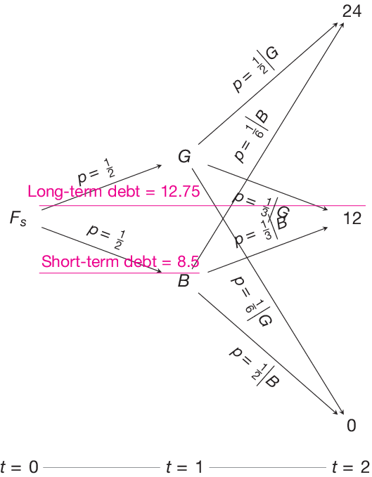


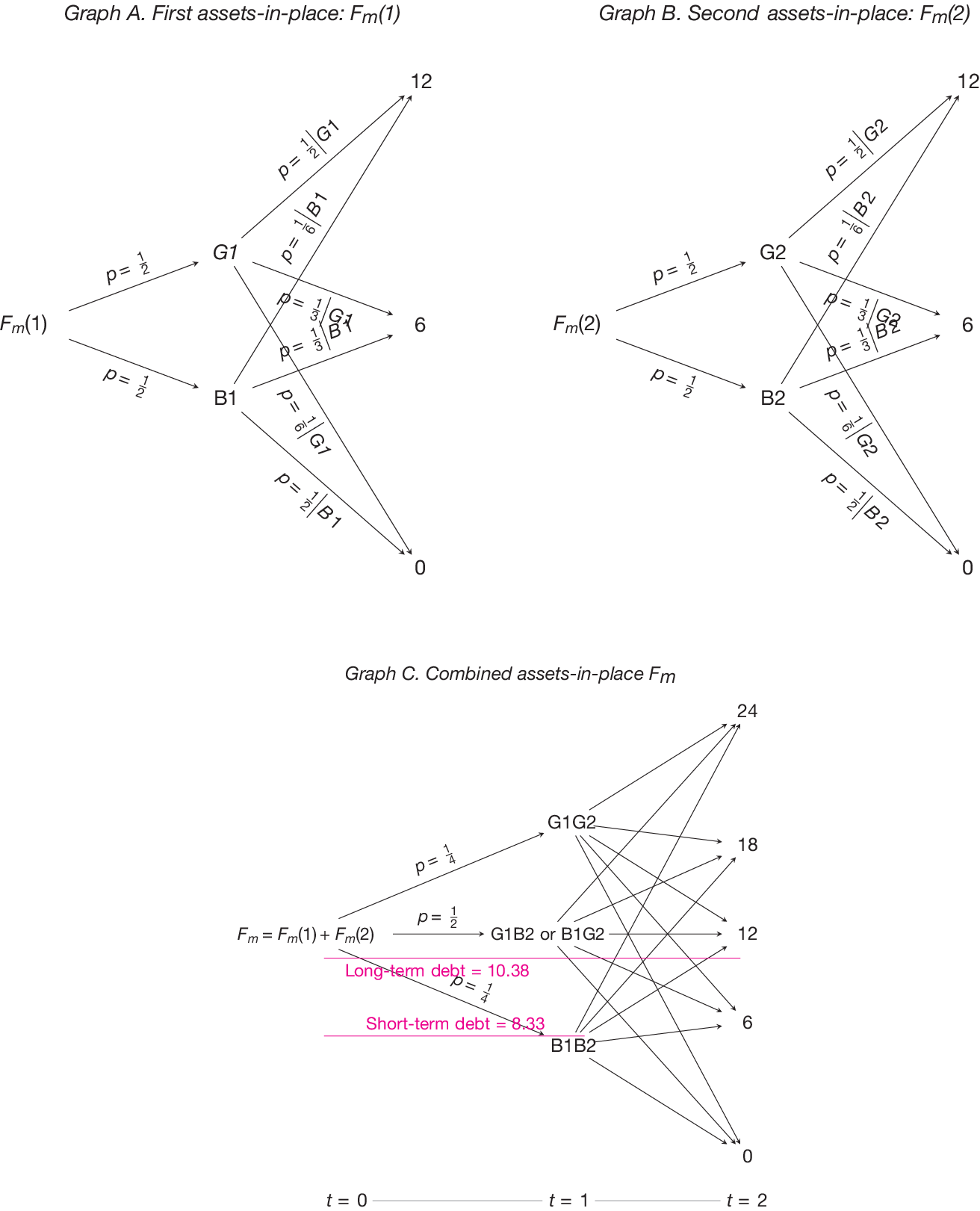


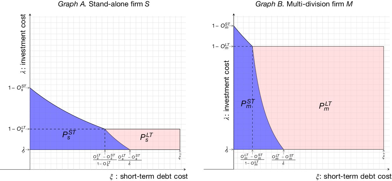




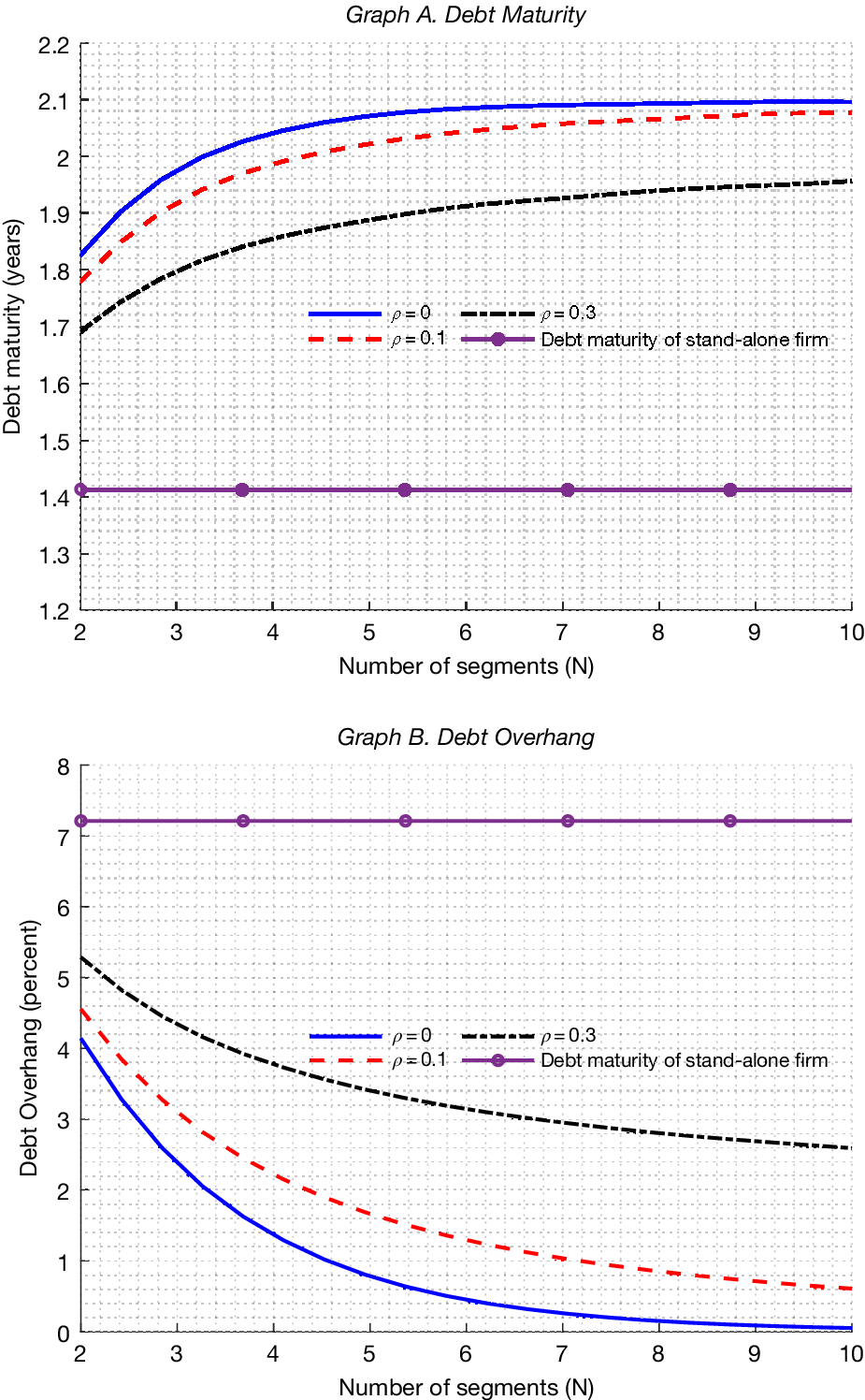


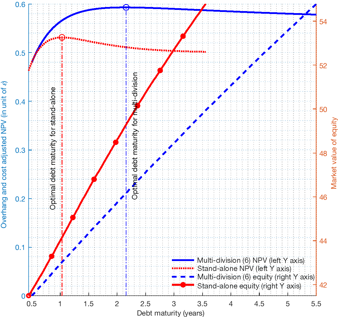


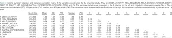
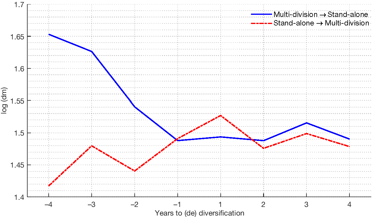
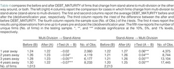
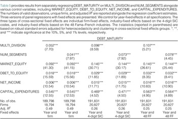
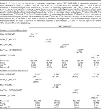
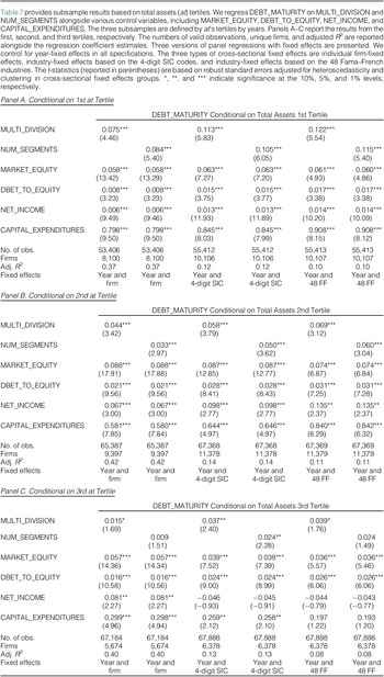
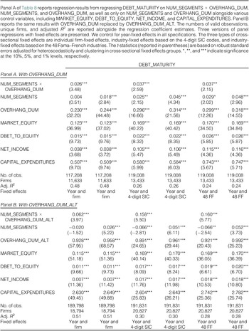
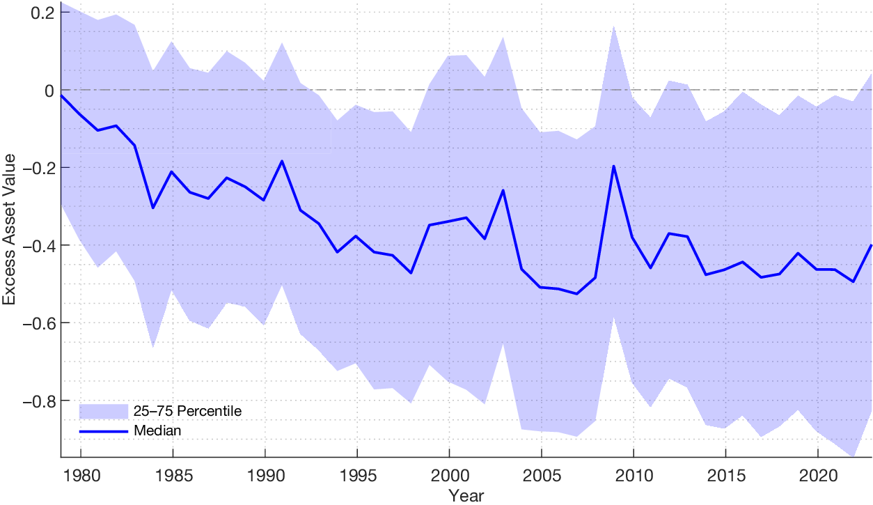


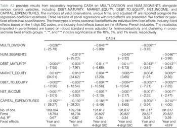


 Open access

