

I. Introduction
A central question for policymakers is whether the economic effects of climate change originate on the supply side—through reductions in productive capacity, labor productivity, and operational resilience—or mostly reflect demand-side responses. This distinction matters for the design of policies: Supply-driven effects call for fiscal support and structural policies that strengthen productive capacity and firm resilience, whereas demand-driven effects are better addressed through monetary policy. In this article, we identify the supply-side effect of temperature shocks on firm sales using an identification strategy that isolates supply-side variation within production networks.
Existing evidence establishes that temperature shocks can have important economic effects but provides limited guidance on whether these effects operate through the supply or demand side of the economy. Early cross-sectional evidence shows that countries with higher temperatures tend to have lower income (Gallup, Sachs, and Mellinger (Reference Gallup, Sachs and Mellinger1999), Dell, Jones, and Olken (Reference Dell, Jones and Olken2009)), and subsequent work documents negative effects of temperature on aggregate economic activity and labor productivity (Hsiang (Reference Hsiang2010), Dell, Jones, and Olken (Reference Dell, Jones and Olken2012), and Graff-Zivin and Neidell (Reference Graff-Zivin and Neidell2014)). At the firm level, however, evidence on sales is less conclusive: Pankratz, Bauer, and Derwall (Reference Pankratz, Bauer and Derwall2023) find negative effects, whereas Addoum, Ng, and Ortiz-Bobea (Reference Addoum, Ng and Ortiz-Bobea2020), (Reference Addoum, Ng and Ortiz-Bobea2023) find limited average effects and significant cross-industry heterogeneity. One reason for these mixed findings may be that temperature shocks simultaneously affect firms’ productive capacity and the demand they face. Existing estimates that do not separate these channels therefore need not recover the underlying supply-side effect. We address this identification challenge by exploiting production networks to isolate variation in firm sales that originates from temperature-induced supply disruptions.
Identifying supply-side effects is empirically challenging not only because weather shocks affect both supply and demand at the same time but also because many firms are geographically clustered with their suppliers, leading to correlated exposure (Ellison and Glaeser (Reference Ellison and Glaeser1997)). In this article, we estimate supply-side effects by leveraging a data set that combines supplier-by-customer sales data for the production network of publicly traded nonfinancial U.S. firms (sourced from the Compustat segment files) with the precise location of suppliers’ headquarters and establishments (from Compustat and the National Establishment Time Series (NETS)) and high-resolution temperature and precipitation data for the United States (from the PRISM Climate Group). Following an identification strategy similar to Khwaja and Mian (Reference Khwaja and Mian2008), we introduce client-by-year (or supplier-industry-by-client-by-year) fixed effects in our empirical specifications to hold demand fixed while comparing sales to the same client in the same year across suppliers exposed to different temperature shocks. We proxy the suppliers’ exposure to the local temperature both through the location of their main headquarters and through the average exposure of the suppliers’ establishments to local temperature.
We find that higher local temperatures significantly reduce supplier sales relative to other suppliers serving the same client, indicating economically meaningful supply-side effects. A 1°C increase in average local temperature leads to about a 2.5% decline in annual supplier sales relative to other suppliers serving the same client, with stronger effects in manufacturing and other heat-sensitive industries. The effects operate mainly at the intensive margin, as we do not observe systematic termination of supplier–client relationships. Our findings imply that climate policy should devote attention to adaptation measures that strengthen firms’ operational resilience, such as cooling technologies, process innovation, and supply-chain risk management.
The relation between firm sales and average temperature changes may be nonlinear. We investigate whether the effect is heterogeneous across the magnitude of temperature changes and across temperature normals (i.e., long-term historical average temperature). Intuitively, larger and more unusual increases in average temperatures are likely to be more disruptive to firms than smaller changes. Consistent with this idea, we expect larger declines in sales among firms experiencing larger increases in average temperature. Our results show that firms exposed to average temperature changes in the top quintile of the distribution experience a 4.3%–5.9% greater decline in sales than those in the bottom quintile. We also expect the effects to be more pronounced for firms located in areas that do not typically experience warm weather. Firms in regions with baseline temperatures below the median, or in areas with larger deviations from normal temperatures, exhibit a 2.5%–3.1% greater reduction in sales for each 1°C increase in average local temperature.
Our main identifying assumption is that differences in sales growth between the treatment group (i.e., suppliers exposed to a change in the average temperature) and the control group would have followed parallel trends in the absence of the treatment (i.e., weather shocks). We find no evidence of preexisting differential trends in sales growth between groups of suppliers. Our identification strategy also requires that local temperature changes are exogenous to the suppliers’ activity. Although it is unequivocal that the real activity of specific firms and industries, particularly in CO2-intensive industries, affects climate (Intergovernmental Panel on Climate Change (2023)), such an impact is at the global level rather than at the firm-specific or local level. We interpret our coefficients as capturing supply-side effects, as the variation in sales is driven by suppliers’ exposure to changes in average temperatures. Nevertheless, our estimates may also partly reflect demand-side responses if clients anticipate disruptions at exposed suppliers and reallocate purchases toward alternative suppliers in response to expected price increases, delivery delays, or deterioration in supplier reliability.
A potential concern with our main estimates is the standard trade-off between internal and external validity. Controlling for demand requires restricting the sample to firms with at least two suppliers and excluding firms that sell directly to end consumers. However, these concerns are unlikely to be consequential in our context for the following reasons. First, excluding firms with only a single supplier has a limited impact on sample size, reducing the number of unique suppliers from 1,774 to 1,405. Second, business-to-business transactions (on which our sample is based) account for a substantial share of economic activity, representing approximately 75% of total final consumption.Footnote 1 Finally, as we explain subsequently, the mechanisms we uncover suggest supply-side disruptions are largely independent of whether the final customers are other businesses or end consumers. Nevertheless, we address this concern by reweighting our observations using inverse probability weights based on total sales in each 2-digit SIC industry to better reflect the broader firm-level population. Our main results remain quantitatively similar.
Next, we investigate four nonmutually exclusive mechanisms through which changes in temperature can affect firm sales. The first mechanism is labor productivity and labor supply. Our results are more pronounced for manufacturing firms, firms in heat-sensitive industries (i.e., firms in industries with outdoor activities or manufacturing processes), and firms with higher labor intensity (as proxied by the ratio of the number of employees to assets). This is consistent with the idea that higher temperatures lower labor productivity due to absenteeism and more challenging working conditions (Graff-Zivin and Neidell (Reference Graff-Zivin and Neidell2014)).
The second mechanism is financial constraints. Financially constrained firms may be unable to adapt due to their lack of funding and inability to raise financing to absorb higher costs and investment associated with weather shocks. In contrast, unconstrained firms can better cover the costs and make the investments necessary to mitigate the adverse effects of climate change (e.g., Gourio and Fries (Reference Gourio and Fries2020), Fried (Reference Fried2022)). Our proxies for financial constraints are credit rating, payout ratio, and the financial constraints composite index of Bartram, Hou, and Kim (Reference Bartram, Hou and Kim2022). We find that the effect of changes in temperature on financially constrained firms is larger than that on unconstrained firms. Our results suggest that financially constrained firms have limited financial resources to overcome weather shocks without affecting sales. These results are consistent with Giroud and Mueller (Reference Giroud and Mueller2019), who find that the propagation of economic shocks through firms’ internal networks is more pronounced for financially constrained firms.
The third mechanism is operational flexibility. Larger and diversified firms can use their internal networks to reallocate resources across their business and geographic segments to respond and adapt to weather shocks. In line with this mechanism, the estimates indicate that the effect of higher temperature on firm sales is larger for firms with establishments in fewer counties and for firms with less diversified operations. These results suggest that geographic and business diversification can mitigate the effects of temperature changes.
The fourth mechanism is switching costs. Barrot and Sauvagnat (Reference Barrot and Sauvagnat2016) show that switching costs between trade partners due to input specificity are substantial and can explain the propagation of shocks in production networks. We proxy for input specificity and switching costs at the supplier level using the market value of patents and an indicator for industries that sell standardized goods. These measures capture the importance of relationship-specific investments and restrictions on sourcing alternative suppliers. We find that the reduction in sales is more pronounced for suppliers that are more easily substitutable (i.e., those providing standardized inputs and lower-value patents). These findings are consistent with the idea that the supplier-specific economic costs of weather shocks are larger when switching costs are lower.
We next examine whether firms can mitigate the adverse effects of temperature shocks through adaptation. Guided by the mechanisms underlying our findings, we focus on three strategies that may enhance firms’ resilience: automation, geographic diversification of production, and investment. We find no significant decline in sales following temperature shocks among firms that have recently automated production, expanded their geographic footprint by opening plants in other counties, or increased investment. In contrast, firms that have not adopted these strategies experience substantial declines in sales. These results suggest that firms can mitigate their exposure to temperature shocks by investing in technologies and production structures that increase operational resilience.
We then examine how operational and financial constraints influence firms’ ability to adapt. Focusing on automation, proxied as substitution away from heat-sensitive labor, we find that firms that are less operationally or financially constrained are more likely to adopt adaptive strategies. In contrast, constrained firms face a dual challenge: They are both more exposed to temperature shocks and less capable of responding effectively. These findings highlight a key policy priority: supporting operationally and financially constrained firms that lack the resources to adapt independently to climate risks (Fankhauser and Soare (Reference Fankhauser and Soare2013)).
We contribute to several strands of the literature. First, we contribute to the literature on the real economic costs of climate change. Initial cross-sectional studies show that countries with higher average temperatures tend to have lower income (Gallup et al. (Reference Gallup, Sachs and Mellinger1999), Dell et al. (Reference Dell, Jones and Olken2009)). More recent work documents similarly adverse effects of higher temperatures on aggregate economic activity (Hsiang (Reference Hsiang2010), Jones and Olken (Reference Jones and Olken2010), and Dell et al. (Reference Dell, Jones and Olken2012)). Using a worldwide sample, Pankratz et al. (Reference Pankratz, Bauer and Derwall2023) find that increased exposure to extremely high temperatures reduces firms’ revenues and operating income. In contrast, Addoum et al. (Reference Addoum, Ng and Ortiz-Bobea2020) find that the effect of temperature exposure on firm sales is not significant using establishment-level and firm-level data in the United States. In subsequent work, Addoum et al. (Reference Addoum, Ng and Ortiz-Bobea2023) find that extreme temperatures have heterogeneous effects as some industries suffer whereas others benefit. In short, although previous research documents negative effects of climate change on aggregate economic activity and labor productivity, evidence on firm-level sales and performance is mixed.
There is also evidence that climate change and related phenomena, such as pollution and carbon emissions, increase the consumption of energy and other goods, including air conditioning, air purifiers, and medicine (e.g., Deschênes, Greenstone, and Shapiro (Reference Deschênes, Greenstone and Shapiro2017), Abel, Holloway, Harkey, Meier, Ahl, Limaye, and Patz (Reference Abel, Holloway, Harkey, Meier, Ahl, Limaye and Patz2018), and Ito and Zhang (Reference Ito and Zhang2020)). Relatedly, Benmir, Jaccard, and Vermandel (Reference Benmir, Jaccard and Vermandel2021) propose a model in which environmental externalities raise households’ willingness to consume goods. This is the first article to isolate the supply-side effects of climate change on firm sales using granular data and high-dimensional fixed effects. This is important because demand-side variation is a confounder and may be ambiguous and heterogeneous across regions and industries. Other articles also rely on high-dimensional fixed effects to exploit geographic differences in exposure to temperature. For example, Jones and Olken (Reference Jones and Olken2010) use product-year fixed effects and, thus, exploit differences in temperature across countries that control for global changes in demand for each product. The higher degree of granularity in our data allows us to further improve identification by controlling for local changes in demand, which can be affected by local climate and weather conditions. This approach allows us to identify supply-side effects of changes in temperature after purging firm-specific demand effects. Our results show that the supply-side effects of temperature changes on firm sales are substantial and help explain the apparent puzzle of why average temperature affects labor productivity but not firm sales or performance.
Second, we contribute to the literature on the effects of temperature extremes on firm output through labor productivity. Graff-Zivin and Neidell (Reference Graff-Zivin and Neidell2014) show that extremely hot temperatures reduce hours worked across several heat-sensitive industries. Somanathan et al. (Reference Somanathan, Somanathan, Sudarshan and Tewari2021) find reduced worker productivity on hot days, which can decrease plant annual output by 2% per degree Celsius. In related work, Zhang, Deschênes, Meng, and Zhang (Reference Zhang, Deschênes, Meng and Zhang2018), Chen, Huynh, and Zhang (Reference Chen, Huynh and Zhang2019), and Colmer et al. (Reference Colmer, Martin, Muuls and Wagner2019) show that higher local temperature lowers total factor productivity, value added, and employment in manufacturing using establishment-level or firm-level data. Xiao (Reference Xiao2024), (Reference Xiao2026) shows that extreme heat reduces labor productivity and discourages both firm and job creation, especially in heat-sensitive industries. We contribute to this literature by identifying the mechanisms that drive these supply-side effects and how firms adapt to these shocks. Our results suggest that the decline in sales can be due to lower labor productivity and labor supply, lack of operational flexibility or financial resources to adapt the productive processes, and clients’ inability to switch to nonaffected suppliers. Importantly, we show that firms that adapt to higher temperatures (e.g., through automation, geographical diversification, or increasing investments) can mitigate the negative effects of higher temperatures.
Finally, our evidence is complementary to research studying the propagation of weather shocks along the supply chain from the supplier to its clients. Barrot and Sauvagnat (Reference Barrot and Sauvagnat2016) find that suppliers affected by major natural disasters in the United States lead to output losses for their clients, especially when they produce a specific input. Carvalho, Nirei, Saito, and Tahbaz-Salehi (Reference Carvalho, Nirei, Saito and Tahbaz-Salehi2021) find that downstream propagation explains a sizable fraction of the decline in gross output following the Great East Japan Earthquake of 2011. Pankratz and Schiller (Reference Pankratz and Schiller2024) show that heat waves and flooding at supplier locations reduce the operating performance of their customers in global supply chains. In contrast to these studies, which examine the downstream propagation of natural disaster shocks, our articles uses production networks as a laboratory to estimate the impact of changes in average temperature on firm sales while controlling for firm-specific demand.
II. Data and Methodology
A. Sample and Variables
Our sample consists of supplier–client pairs with headquarters in the United States. Regulations SFAS 14 and 131 require publicly listed firms in the United States to disclose, annually, the identity of clients and the sales to clients whose purchases represent more than 10% of total sales.Footnote 2 We obtain data on supplier–client links and associated sales from the WRDS Supply Chain database (Compustat Segment IDs) for the 2000–2018 period. This WRDS analytics tool is built on the historical customer segment data and complemented by data contributed by researchers, including Cohen and Frazzini (Reference Cohen and Frazzini2008) and Cen, Maydew, Zhang, and Zuo (Reference Cen, Maydew, Zhang and Zuo2017). As we restrict the sample to publicly traded firms in Compustat, we cannot identify clients that are private firms, government entities, or firms based outside the United States. We exclude suppliers that are regulated utilities (SIC codes 4900–4999), financial firms (SIC codes 6000–6999), or public administration (SIC codes 9100–9729).
We obtain temperature and precipitation data from the PRISM Climate Group (2019). PRISM provides climate observations from weather stations across the continental United States and uses sophisticated climate modeling techniques to interpolate weather data for each 4 × 4 km2 grid (Daly and Bryant (Reference Daly and Bryant2013)). The interpolation method takes elevation, slope orientation, wind direction, rain shadows, terrain complexity, proximity to coastlines and location of temperature inversions, and cold air pools into account. This results in a balanced panel of weather data for the continental United States.
We map the weather grids in PRISM locations to ZIP codes in the U.S. Census Bureau files. We compute the average daily temperature and precipitation at the ZIP code level for each year. Figure 1 plots the change in average daily temperature aggregated per county and year over the sample period. We match the weather variables for each ZIP code to the firms in Compustat using the location of the firm’s main headquarters and the firm’s fiscal year-end. Because a firm’s production plants and sales locations are not always located in the same ZIP code or county as their headquarters (Campello, Connolly, Kankanhalli, and Steiner (Reference Campello, Connolly, Kankanhalli and Steiner2022)), this proxy of the exposure to temperature could be prone to measurement error. We address this issue by obtaining information on the exact location of the firms’ establishments, which we source from the National Establishment Time-Series (NETS) Database produced by Walls & Associates. We calculate a firm-level exposure to temperature by mapping the temperature in each ZIP code to the location of each establishment and averaging the changes in temperature across establishments using the number of employees by establishment as weights. The average change in temperature across establishments is highly correlated with the headquarters-level measure, with a correlation coefficient of 0.86.
Figure 1 plots changes in average daily temperature at the county level. Temperature is averaged by calendar year over the period 2000–2018.

FIGURE 1 Long description
A choropleth map uses a color scale to represent temperature change values. A legend in the Southwest corner shows a gradient from dark red (0.03 to 0.12) to dark blue (-0.15 to -0.08).
* The West and Southwest regions are dominated by dark red and red shades, indicating the highest increases in average daily temperature.
* The Northern and Midwestern regions, particularly around the Great Lakes and Northern Plains, are shaded in dark blue and light blue, indicating a decrease in average daily temperature.
* The Southeast and Mid-Atlantic regions show a mix of light red and dark red, with a notable concentration of dark red in Florida and parts of the Deep South.
* The Northeast displays a transition from light blue in the North to light red and white (neutral change) toward the South.
We obtain extreme weather events data from the National Oceanic and Atmospheric Administration (NOAA) Storm Events Database (NOAA (2025)). This database records the occurrence of significant weather events that have sufficient intensity to cause loss of life, injuries, significant property damage, and/or disruption to commerce.
B. Methodology
Our main objective is to examine whether changes in local temperature affect firms’ sales. To investigate this hypothesis, we estimate the following regression equation:

The dependent variable measures the annual growth rate in supplier
$ i $
 ’s sales to client
$ j $
 between years t – 1 and t.
Footnote
3 The main independent variable,
$ \Delta \;{Temp}_{it} $
 , is the change in average daily temperature in degrees Celsius in the ZIP code where supplier
$ i $
 ’s headquarters is located from year t – 1 to year t. Following the climate economics literature (e.g., Dell, Jones, and Olken (Reference Dell, Jones and Olken2014)), we include the average daily precipitation in millimeters in the ZIP code where supplier i headquarters is located from year t – 1 to year t (
$ {Prcp}_{it} $
 ). In all specifications, we add a set of lagged supplier characteristics,
$ {X}_{it-1} $
 , which include firm size as proxied by total assets (Assets), the ratio of the market value of assets to book value of assets (Tobin’s Q), the ratio of cash and equivalents to assets (Cash), the ratio of total debt to market value of assets (Leverage), and the ratio of net property, plant, and equipment to total assets (Tangibility).
Our client–supplier pair data allow us to include client-by-year fixed effects,
$ {\delta}_{jt} $
 , in the regressions. Therefore, identification comes from the variation in the change in temperature across the suppliers of a given client in the same year. As shown by Khwaja and Mian (Reference Khwaja and Mian2008) in the context of shocks to credit supply, firm-by-year fixed effects absorb all unobserved heterogeneity at the firm level in a given year. Thus, we will compare the changes in business transactions across suppliers selling to the same firm. For this reason, our results are unlikely to be driven by changes in aggregate firm-specific demand.Footnote
4 The estimated difference in sales can therefore be plausibly attributed to supply-side factors, such as changes in labor supply, changes in productivity, or increases in operating costs. In addition, weather shocks can affect the quality of products or delay deliveries to clients.Footnote
5 We also estimate a more stringent specification, which includes (supplier) industry-by-client-by-year fixed effects to absorb time-varying differences across suppliers in the same industry (2-digit SIC) that sell to the same firm.
The main coefficient of interest is
$ {\beta}_1 $
 , which estimates the effect of changes in temperature on firm sales. A negative
$ {\beta}_1 $
 would indicate that firms suffering increases in average daily temperature reduce their sales by larger amounts than otherwise similar firms selling to the same client. In our baseline regressions, we cluster the standard errors at the county level (based on the supplier’s headquarters) as firms located in the same region are exposed to correlated weather shocks. The Appendix provides variable definitions and data sources.
C. Summary Statistics
Panel A of Table 1 contains a year-by-year description of our sample. Our sample consists of 10,730 supplier–client-year observations for 1,405 unique suppliers and 331 unique clients over the period 2000–2018, with about 560 observations per year on average. Sales to clients in our sample account, on average, for 38% of the total sales of sample firms. Panel A also reports that the coefficient of our variable of interest is estimated using the variation in the change in temperature of about five suppliers per client. Table 1 also reports time-series variation in the average daily temperatures in the ZIP codes where firms are located, ranging from −1.1°C to 0.97°C. The average temperature in the firms’ headquarters is similar to that of the establishment-weighted temperature variable, which is consistent with most of the production of firms taking place at the firm’s headquarters or in establishments that are located close to the headquarters.

TABLE 1 Long description
The table is divided into three panels.
Panel A. Sample by Year:
This panel tracks data from 2000 to 2018. Key columns include Number of Observations, Unique Suppliers, Unique Clients, Average Number of Suppliers per Client, Average Supplier Sales Coverage, and Average Temperature/Change in Temperature at Supplier Headquarters and Establishments.
- In 2000, there were 414 observations with 291 unique suppliers and 94 unique clients.
- By 2018, observations were 439 with 271 unique suppliers and 98 unique clients.
- The total unique observations across the period are 10,730, with 1,405 unique suppliers and 331 unique clients.
- The overall average number of suppliers per client is 4.8, and the average supplier sales coverage is 0.377.
Panel B. Suppliers:
This panel provides descriptive statistics (Mean, 25th Percentile, Median, 75th Percentile, Standard Deviation, and Number of Observations) for supplier variables.
- Delta log(Sales) has a mean of 0.016.
- Delta Temp has a mean of minus 0.001.
- Temp has a mean of 14.061.
- log(Assets) has a mean of 5.954.
- Other variables include Tobin’s Q (mean 1.995), Cash (mean 0.244), Leverage (mean 0.140), and weather-related indicators like Cold/windchill, Heavy snow, Heat, Hot days, Heavy rain, and Flood.
- Automation patent application has a mean of 0.306 based on 8,916 observations.
Panel C. Clients:
This panel provides the same descriptive statistics for client variables.
- Temp has a mean of 13.998.
- Temp sub Est. emp.-weighted has a mean of 12.402.
- log(Assets) has a mean of 10.756.
- Tobin’s Q has a mean of 1.807.
- Cash has a mean of 0.104.
- Leverage has a mean of 0.174.
- Tangibility has a mean of 0.289.
Panels B and C of Table 1, respectively, contain descriptive statistics for the supplier and client firms in our pair-level sample. Client firms are larger than supplier firms in terms of total assets. This is due to regulation SFAS 14, which only requires the disclosure of the names of clients that account for at least 10% of total sales. Client firms are more leveraged, hold less cash, have more tangible assets, and have a lower Tobin’s Q than supplier firms. Consistent with a high degree of geographic colocation of suppliers and clients, the average levels of temperature are similar for client and supplier firms.
D. Identifying Assumptions
An identifying assumption in our estimates is that local temperature changes are exogenous to the suppliers’ business transactions or sales. Although business transactions among certain firms and industries, particularly in CO2-intensive sectors, may have a significant effect on climate, this effect operates at the global level rather than the local level. For example, the areas most affected by climate change are often those with lower levels of industrialization and economic development. Therefore, it is difficult to argue that an individual firm’s business transactions affect the local temperature. Another assumption is that the sales response for a firm’s products or services would have been the same for the treatment group (i.e., suppliers exposed to a change in the average temperature) and the control group absent the weather shocks (i.e., changes in the average temperature). We assess whether the parallel trends assumption is plausible using pretreatment observations.
Our identification strategy exploits within-client-year variation in temperature across a client’s suppliers. This approach follows Khwaja and Mian (Reference Khwaja and Mian2008) in using client-by-year fixed effects to identify supply-side shocks. Paravisini, Rappoport, and Schnabl (Reference Paravisini, Rappoport and Schnabl2023) argue that an additional identifying assumption of this empirical strategy is that changes in a firm’s credit demand are equally spread across all the banks lending to the firm. In our case, this implies that changes in clients’ purchases are equally spread across all suppliers, which is more plausible when suppliers are from the same industry. For this reason, we estimate specifications that include supplier industry-by-client-by-year fixed effects, restricting the variation to suppliers within the same industry selling to the same client in each period.
III. Results
A. Average Temperature
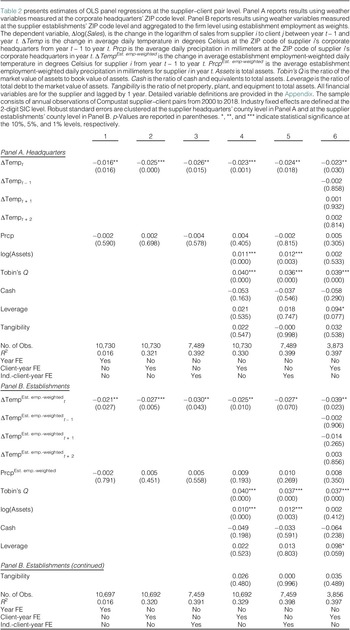
Table 2 presents the estimates of the effect of changes in average temperature on changes in firm sales using the regression in equation (1). Panel A reports estimates using changes in temperature in the firm’s headquarters location at the ZIP code level. Panel B reports estimates using establishment-level changes in temperature (at the ZIP code level) weighted by the number of employees by establishment. We estimate the regressions using three different sets of fixed effects: year fixed effects in column 1; client-by-year fixed effects in columns 2, 4, and 6; and supplier industry-by-client-by-year fixed effects in columns 3 and 5. In addition, the regressions in columns 4–6 include firm-level control variables.

TABLE 2 Long description
The table presents O L S panel regressions for Delta log Sales.
Panel A (Headquarters) focuses on weather at corporate headquarters.
* Delta Temp sub t shows negative coefficients across all models, ranging from -0.016 to -0.026, significant at the 1% or 5% levels.
* Lead and lag temperature variables (t minus 1, t plus 1, t plus 2) in model 6 are statistically insignificant.
* Prcp (precipitation) is insignificant across all models.
* Control variables include log Assets, Tobin’s Q, Cash, Leverage, and Tangibility. Tobin’s Q is consistently positive and significant at the 1% level (0.036 to 0.040).
* R-squared values increase from 0.016 in model 1 to approximately 0.39 in models 3, 5, and 6.
Panel B (Establishments) uses employment-weighted weather variables at the establishment level.
* Delta Temp super Est. emp.-weighted sub t shows negative coefficients ranging from -0.021 to -0.039, significant at the 1%, 5%, or 10% levels.
* Similar to Panel A, lead and lag temperature variables are insignificant.
* Prcp super Est. emp.-weighted is insignificant.
* Control variable trends for Tobin’s Q and log Assets mirror Panel A.
* Fixed Effects (F E) vary by model: Model 1 uses Year F E; Models 2, 4, and 6 use Client-year F E; Models 3 and 5 use Ind.-client-year F E.
The results show that the coefficient on changes in average temperature (∆Temp) is negative and statistically significant across all specifications. The estimates in Panel A indicate that a 1°C yearly increase in the average temperature in the supplier’s headquarters ZIP code leads to a 1.6%–2.6% reduction in sales. A similar pattern emerges in Panel B, where estimates are larger in absolute value, ranging from −2.1% to −3.9%.
Columns 1–3 in both Panels A and B of Table 2 report that the inclusion of client-by-year or supplier-industry-by-client-by-year fixed effects, which absorb demand-side variation at the client-year level, magnifies the negative effect of temperature on firm sales by approximately 1 percentage point. Columns 4 and 5 report that including firm-level control variables does not significantly impact the estimated ∆Temp coefficient.
These results are consistent with demand-side variation masking supply-driven sales losses in firm-level estimates; we do not identify the sign or magnitude of this demand-side variation. Our results help to understand why the literature has found negative effects of higher temperature on aggregate economic activity and labor productivity (e.g., Hsiang (Reference Hsiang2010), Dell et al. (Reference Dell, Jones and Olken2012), Graff-Zivin and Neidell (Reference Graff-Zivin and Neidell2014), and Somanathan et al. (Reference Somanathan, Somanathan, Sudarshan and Tewari2021)) but no overall effects on firm-level sales and performance (Addoum et al. (Reference Addoum, Ng and Ortiz-Bobea2020)).
Column 6 in Panels A and B of Table 2 reports the dynamic effects of temperature by including lags and leads of the change in temperature (∆Temp). We find that the negative effect of temperature is significant only in the year of the temperature shock but not before or after. This result supports the assumptions of our identification strategy, as there is no evidence of preexisting differential trends between treated and control groups. In addition, the effect on firm sales is not persistent, consistent with firms’ ability to adapt in the long run.
In Table 3, we examine whether temperature affects firms’ business transactions in a nonlinear way by estimating equation (1) using dummy variables to identify the temperature change quintiles (with the first quintile omitted). As in Table 2, Panel A reports results using temperature exposure in the firms’ headquarters, whereas Panel B uses temperature exposure based on firms’ establishments. The results show that the effects are concentrated in the highest temperature-change quintile (Q5), consistent with a nonlinear effect of temperature on firms’ sales. In fact, firms exposed to average temperature changes in the top quintile of the distribution experience a 4.3%–5.9% greater decline in sales relative to those in the bottom quintile. Thus, the effect of temperature changes on firm sales is more pronounced in locations where the increase in average temperature is more extreme.

TABLE 3 Long description
Panel A (Headquarters) shows regression results for weather at corporate headquarters.
* Delta Temp Q 2: Coefficients range from -0.011 to 0.016, none statistically significant.
* Delta Temp Q 3: Coefficients range from -0.036 to -0.024, with significance at 5 percent in columns 1 and 4.
* Delta Temp Q 4: Coefficients range from -0.033 to -0.011, with significance at 10 percent in column 1.
* Delta Temp Q 5: Coefficients range from -0.059 to -0.043, all significant at 1 percent or 5 percent levels.
* Prcp: Coefficients range from -0.003 to 0.004, none significant.
* Model statistics: Number of observations range from 7,489 to 10,730. R-squared values range from 0.016 to 0.400.
Panel B (Establishments) shows results using employment-weighted weather variables.
* Delta Temp Est. emp.-weighted Q 2: Coefficients range from -0.003 to 0.009, none significant.
* Delta Temp Est. emp.-weighted Q 3: Coefficients range from -0.061 to -0.033, significant at 10 percent in most columns.
* Delta Temp Est. emp.-weighted Q 4: Coefficients range from -0.039 to -0.027, none significant.
* Delta Temp Est. emp.-weighted Q 5: Coefficients range from -0.054 to -0.037, significant at 5 percent or 10 percent levels.
* Prcp Est. emp.-weighted: Coefficients range from -0.002 to 0.008, none significant.
* Model statistics: Number of observations range from 7,459 to 10,697. R-squared values range from 0.016 to 0.399.
Both panels include fixed effects (F E) for Year, Client-year, or Industry-client-year as indicated in the bottom rows.
The effect of temperature on a firm’s sales can also depend on the local climate and weather conditions. We expect the disruptive effects to be more pronounced for firms in areas that do not typically experience warm weather or large deviations in temperatures, as firms in these locations might not be prepared to deal with high temperatures or large temperature swings. We analyze the effect of local climate by estimating our specifications separately for firms located in areas with i) average daily temperatures in each year below and above the median and ii) temperature normals, defined as the long-term (30-year) averages over the period from 1981 to 2010 (drawn from PRISM) below and above the median.
Panel A of Table 4 presents these estimates using the specification in column 4 of Table 2. In columns 1 and 2, we find that the disruptive effects of temperature are larger for firms in areas with average temperatures below the median, with an estimated impact of −3.2%. In columns 3 and 4, we find the negative effect of temperature is significantly stronger (−3.2%) in areas with below-median normal temperatures.

TABLE 4 Long description
The table is divided into three panels, each containing four columns of regression results. The dependent variable for all regressions is the change in the logarithm of sales.
Panel A. Local Climate:
- Columns 1 and 2 compare Low vs High Average Temperature. Delta Temp is -0.032 (p-value 0.016, significant at 5 percent) for Low and -0.022 (p-value 0.144) for High.
- Columns 3 and 4 compare Low vs High Temperature Normal. Delta Temp is -0.032 (p-value 0.015, significant at 5 percent) for Low and -0.016 (p-value 0.269) for High.
- P r c p (precipitation) is near zero and statistically insignificant across all columns.
- Number of observations ranges from 4,700 to 4,753 with R-squared values between 0.357 and 0.388.
Panel B. Summer Temperatures:
- Columns 1 and 2 use Calendar months. Delta Temp is -0.031 (p-value 0.012, significant at 5 percent) for Low and -0.012 (p-value 0.495) for High.
- Columns 3 and 4 use Average Normal months, showing identical results to the calendar month columns.
- P r c p remains insignificant.
- Number of observations is 4,709 or 4,758 with R-squared values between 0.358 and 0.386.
Panel C. Deviations from Normal:
- Columns 1 and 2 compare Low vs High Positive Deviations. Delta Temp is -0.023 (p-value 0.156) for Low and -0.029 (p-value 0.011, significant at 5 percent) for High.
- Columns 3 and 4 compare Low vs High Absolute Deviations. Delta Temp is -0.008 (p-value 0.540) for Low and -0.027 (p-value 0.009, significant at 1 percent) for High.
- P r c p remains insignificant.
- Number of observations ranges from 4,673 to 4,775 with R-squared values between 0.353 and 0.377.
All panels include Controls and Client-year F E (fixed effects).
We also examine the effect of seasonal variation by focusing on summer temperatures, as high temperatures usually occur during the summer. In columns 1 and 2 in Panel B of Table 4, we define summer using the meteorological definition (i.e., from June to August). In columns 3 and 4, we define summer as the 3 months with the highest monthly temperature normal (long-term average). This alternative definition allows for differences in weather conditions across the continental United States. Under both definitions of summer, our results show that the negative effects of temperature on firm sales are more pronounced (−3.1%) for firms in areas with summer temperatures below the median.
We assess the effect of temperature swings by examining deviations from the temperature normal. In columns 1 and 2 in Panel C of Table 4, we examine the average positive deviations from the temperature normal. A higher positive deviation implies that the location experiences a hotter year relative to its long-run average temperature.Footnote 6 In columns 3 and 4, we examine the average absolute deviations from normal.Footnote 7 A higher absolute deviation implies that the location experiences a year with larger deviations (both positive and negative) relative to its long-run average temperature. Under both measures of temperature swings, we find that the negative effects of temperature on firm sales are larger for firms in areas with larger deviations from temperature normal, with estimated effects of −2.7% and −2.9% in columns 3 and 4, respectively.
Overall, these results suggest that firms located in areas that are not typically exposed to high temperatures, heat waves, or large temperature swings are less prepared to cope with warmer average temperatures. For example, these firms may lack air conditioning, heat insulation, or heat-resistant infrastructure, or they may be less likely to adopt measures that mitigate the adverse effects of heat, such as shifting workloads to early-morning or late-evening hours.
B. Extreme Weather Events
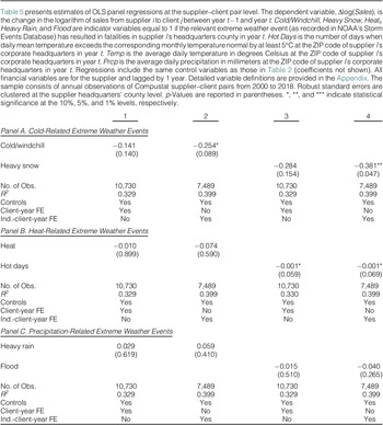
We examine supply-side effects of extreme weather events on firm sales. Table 5 reports the effects of extreme weather events on interfirm sales using the specifications in Table 2. We focus on three sets of extreme weather events that are closely related to climate change: i) cold, ii) heat, and iii) precipitation. To identify weather events recorded in the Storm Events database that are “extreme,” we look at events that result in at least one fatality. These events are rare, with the mean values ranging from 0.0002 (Heavy Snow) to 0.0234 (Flood).

TABLE 5 Long description
The table is divided into three panels: Panel A for cold-related events, Panel B for heat-related events, and Panel C for precipitation-related events. All panels use four columns representing different regression specifications.
Panel A. Cold-Related Extreme Weather Events:
* Cold/windchill: Column 1 shows -0.141 (p-value 0.140); Column 2 shows -0.254* (p-value 0.089).
* Heavy snow: Column 3 shows -0.284 (p-value 0.154); Column 4 shows -0.381** (p-value 0.047).
* Number of observations: 10,730 in columns 1 and 3; 7,489 in columns 2 and 4.
* R-squared: 0.329 in columns 1 and 3; 0.399 in columns 2 and 4.
Panel B. Heat-Related Extreme Weather Events:
* Heat: Column 1 shows -0.010 (p-value 0.899); Column 2 shows -0.074 (p-value 0.590).
* Hot days: Column 3 shows -0.001* (p-value 0.059); Column 4 shows -0.001* (p-value 0.069).
* Number of observations and R-squared values are consistent with Panel A.
Panel C. Precipitation-Related Extreme Weather Events:
* Heavy rain: Column 1 shows 0.029 (p-value 0.619); Column 2 shows 0.059 (p-value 0.410).
* Flood: Column 3 shows -0.015 (p-value 0.510); Column 4 shows -0.040 (p-value 0.265).
Fixed Effects (F E) for all panels:
* Columns 1 and 3 include Client-year F E.
* Columns 2 and 4 include Industry-client-year F E.
* All columns include control variables.
In Panel A of Table 5, we examine the effects of cold-related extreme weather events on firm sales. We find that the coefficients of these extreme weather event indicators range from −0.141 to −0.381, but they are only statistically significant when estimated with industry-by-client-by-year fixed effects.
In Panel B of Table 5, we examine the effects of heat-related extreme weather events. The coefficient of the heat event indicator is negative but not statistically significant. We construct an additional variable, Hot Days, which counts the number of days in which the local temperature exceeds the corresponding monthly normal by more than 5°C. We find that this variable is negative and statistically significant at the 10% level.
In Panel C of Table 5, we examine the effects of precipitation-related extreme weather events. The coefficient of the Heavy Rain indicator is positive, whereas that on the Flood indicator is negative, but neither is statistically significant at conventional levels.
Taken together, we find some evidence of negative effects of extreme cold and heat events on firm sales; however, possibly due to the rarity of such events, the corresponding coefficients are estimated with lower precision.
IV. How Does Temperature Affect Firm Sales?
Our baseline specifications account for demand-side factors (observed and unobserved, time-varying and time-invariant), allowing us to attribute temperature-induced difference in sales to supply-side factors. These factors might include reductions in firm sales due to lower labor supply or productivity (e.g., absenteeism, working conditions, workforce health, and safety) or higher operating costs (e.g., energy or investment costs for air conditioning, building insulation, equipment cooling or heating systems, and higher transportation costs). In addition, weather shocks can affect the quality or the price of products or delay deliveries to clients, which may lead clients to substitute toward unaffected suppliers. In this section, we exploit the heterogeneity in our data to study the mechanisms through which changes in temperature might affect firm supply and which firm characteristics can alleviate or amplify the effect of weather shocks on firm sales.
A. Labor Supply and Productivity
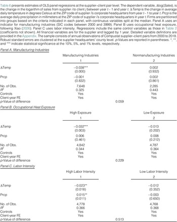
We explore whether the mechanism behind the adverse effects on firm sales documented in the baseline results might be due to lower labor supply and productivity (Graff-Zivin and Neidell (Reference Graff-Zivin and Neidell2014), Zhang et al. (Reference Zhang, Deschênes, Meng and Zhang2018), Chen et al. (Reference Chen, Huynh and Zhang2019), and Colmer et al. (Reference Colmer, Martin, Muuls and Wagner2019)). If this is the case, we expect our estimates to be larger for firms whose labor supply and productivity are most sensitive to weather conditions. We consider three measures to test for this mechanism: i) whether a firm operates in manufacturing, ii) occupational exposure to heat, and iii) labor intensity, proxied by the ratio of employees to assets.
If temperature primarily affects firm performance via a labor productivity channel, manufacturing firms are likely to be more affected. Panel A of Table 6 reports the results split by manufacturing status using the specification in column 4 of Table 2. Column 1 presents the results for manufacturing industries, and column 2 presents the results for other industries. We find that the ∆Temp coefficient is negative and statistically significant with an estimate of −3.8% in manufacturing, whereas the ∆Temp coefficient is not statistically significant for firms in other industries. The difference in coefficients is statistically significant at the 10% level.

TABLE 6 Long description
The table consists of three panels, A, B, and C, each containing O L S panel regressions where the dependent variable is the change in the logarithm of sales.
Panel A. Manufacturing Industries:
- Delta Temp for Manufacturing Industries is minus 0.038 with a p-value of 0.000, significant at the 1 percent level. For Nonmanufacturing, it is 0.002 with a p-value of 0.932.
- Prcp is minus 0.001 for Manufacturing and 0.002 for Nonmanufacturing, both statistically insignificant.
- Number of observations: 7,648 for Manufacturing and 2,285 for Nonmanufacturing.
- R-squared: 0.325 for Manufacturing and 0.443 for Nonmanufacturing.
- p-Value of difference between groups is 0.059.
Panel B. Occupational Heat Exposure:
- Delta Temp for High Exposure is minus 0.032 with a p-value of 0.003, significant at the 1 percent level. For Low Exposure, it is minus 0.013 with a p-value of 0.202.
- Prcp is 0.006 for High Exposure and 0.008 for Low Exposure, both statistically insignificant.
- Number of observations: 4,842 for High Exposure and 4,787 for Low Exposure.
- R-squared: 0.344 for High Exposure and 0.364 for Low Exposure.
- p-Value of difference between groups is 0.229.
Panel C. Labor Intensity:
- Delta Temp for High Labor Intensity is minus 0.023 with a p-value of 0.018, significant at the 5 percent level. For Low Labor Intensity, it is minus 0.012 with a p-value of 0.352.
- Prcp for High Labor Intensity is 0.015 with a p-value of 0.011, significant at the 5 percent level. For Low Labor Intensity, it is minus 0.003 with a p-value of 0.650.
- Number of observations: 4,778 for High Labor Intensity and 4,768 for Low Labor Intensity.
- R-squared: 0.366 for High Labor Intensity and 0.368 for Low Labor Intensity.
- p-Value of difference between groups is 0.513.
All panels include Controls and Client-year F E.
Firms in industries with predominantly outdoor activities or manufacturing processes are expected to be more sensitive to heat. Following Xiao (Reference Xiao2026), we construct a measure of heat exposure based on occupational exposure at the industry level. We aggregate job zone scores from the Occupational Information Network (2024), which measure outdoor exposure to weather per occupation, at the 3-digit SIC and 4-digit NAICS level (based on the crosswalk provided in the Bureau of Labor Statistics’ (2024) Occupational Employment and Wage Statistics). Panel B of Table 6 reports the results split by whether a firm is above or below the median occupation-based heat sensitivity score (at the industry level). Column 1 reports the results for firms with above-median heat exposure, whereas column 2 reports results for firms with below-median heat exposure. The coefficient on ∆Temp is −3.2% and statistically significant for firms with above-median heat exposure. For firms with below-median heat exposure, the coefficient is also negative but not statistically significant. The difference in coefficients is not statistically significant at conventional levels.
Firms with higher labor intensity are expected to be more sensitive because a larger share of their input is labor that can be directly affected by heat, both at work and outside the workplace. Panel C of Table 6 reports the results split by whether a firm is above or below the median of the ratio of the number of employees to assets. Column 1 presents the results for firms with high labor intensity where the ∆Temp coefficient is negative and statistically significant at −2.3%. Column 2 presents the results for firms with low labor intensity where the ∆Temp coefficient is not statistically significant.
In sum, our results support the view that labor supply and productivity mechanisms drive our results as the effect of temperature changes is concentrated in firms potentially more affected by higher average temperatures.
B. Financial Constraints
Disruptions to firms’ production processes might be particularly severe if suppliers are financially constrained and cannot raise financing to absorb the increased costs or investments associated with temperature changes. In contrast, unconstrained firms may be better able to tap capital markets to obtain financing to cope with increases in temperature, for example, by hiring additional workers to offset productivity losses, investing in appropriate equipment or infrastructure, and implementing strategies that reduce the firm’s exposure to higher temperatures.
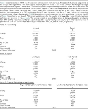
To study this mechanism, we estimate our specification separately across subsamples according to the firms’ financial constraints. We consider three measures of financial constraints: i) whether a firm has a credit rating, ii) whether its payout ratio is above or below the median, and iii) the financial constraints composite index of Bartram et al. (Reference Bartram, Hou and Kim2022).
Table 7 reports the results. Panel A presents the results split by whether a firm is rated by a credit rating agency. Firms with a credit rating have access to public debt markets and, therefore, are less likely to be financially constrained. The ∆Temp coefficient is −3.0% for unrated firms (column 1) and statistically significant. In contrast, there is no statistically significant effect for rated firms (column 2). The difference in coefficients is statistically significant at the 5% level.

TABLE 7 Long description
The table is divided into three panels, each comparing two groups of firms. The dependent variable for all regressions is Delta log Sales.
Panel A. Credit Rating: Compares Unrated (Column 1) and Rated (Column 2) firms. For Delta Temp, the coefficient is -0.030 (p-value 0.000) for Unrated and -0.001 (p-value 0.950) for Rated. Prcp coefficients are 0.006 and -0.009 respectively. Number of observations: 8,346 for Unrated, 1,547 for Rated. R-squared values are 0.340 and 0.439. The p-value of difference is 0.037.
Panel B. Payout: Compares Low Payout (Column 1) and High Payout (Column 2) firms. For Delta Temp, the coefficient is -0.038 (p-value 0.000) for Low Payout and -0.003 (p-value 0.708) for High Payout. Prcp coefficients are 0.006 and 0.001. Number of observations: 5,679 for Low Payout, 3,861 for High Payout. R-squared values are 0.359 and 0.377. The p-value of difference is 0.007.
Panel C. Financial Constraints Composite Index: Compares High Index (Column 1) and Low Index (Column 2) firms. For Delta Temp, the coefficient is -0.039 (p-value 0.001) for High Index and -0.004 (p-value 0.674) for Low Index. Prcp coefficients are 0.009 and -0.003. Number of observations: 4,747 for High Index, 4,817 for Low Index. R-squared values are 0.362 and 0.382. The p-value of difference is 0.013.
All panels indicate that controls and Client-year F E are included.
Panel B of Table 7 measures financial constraints based on whether a firm’s payout ratio is above or below the median. The payout ratio is defined as the sum of common dividends, preferred dividends, and repurchases of common and preferred stock, divided by income before extraordinary items. Firms with a higher payout ratio are considered less financially constrained. Column 1 presents the results for firms with a below-median payout ratio. The coefficient on ∆Temp is −3.8% and statistically significant. In contrast, there is no statistically significant effect for firms with an above-median payout ratio (column 2). The difference in coefficients is statistically significant at the 1% level.
Panel C of Table 7 measures financial constraints using the composite index of Bartram et al. (Reference Bartram, Hou and Kim2022), based on a firm’s KZ index (Kaplan and Zingales (Reference Kaplan and Zingales1997)), WW index (Whited and Wu (Reference Whited and Wu2006)), size-age (SA) index (Hadlock and Pierce (Reference Hadlock and Pierce2010)), size, payout ratio, and credit rating. A firm is assigned to the constrained group if its KZ, WW, or SA index is above the median, if its size or payout ratio is below the median, or if it does not have a credit rating. We then construct the composite financial constraints index by summing the six indicators. A high index value indicates that the firm is more financially constrained. We split the sample into firms with high and low values of the financial constraints composite index based on the median. Column 1 presents the results for firms with a high financial constraints composite index. The coefficient on ∆Temp is −3.9% and statistically significant. In contrast, the coefficient in column 2 for firms with a low financial constraints composite index is not statistically significant. The difference in coefficients is statistically significant at the 5% level.
Overall, the findings support the financial-constraints mechanism and highlight the role of financial constraints in firms’ adaptation to climate change.
C. Operational Constraints
Large firms may be better able to adapt to temperature changes than small firms because economies of scale and scope provide greater operational flexibility and reduce operating constraints. Similarly, geographically diversified firms, as well as conglomerates operating across multiple business segments, may be better able to adapt to temperature changes. Such firms can increase production at unaffected plants or reallocate resources across business segments to offset reductions in activity at affected plants or segments.
Table 8 estimates the effects of temperature changes across different types of firms: small versus large firms, proxied by below- and above-median assets (Panel A); firms operating in a limited number of counties (below median) versus those with more geographically diversified operations (above median; Panel B); and firms with less versus more diversified operations, proxied by above- and below-median Herfindahl–Hirschman Index (HHI) based on establishment sales. The coefficients in column 1 for small firms, firms that operate in a small number of counties, and firms with less diversified operations are negative and statistically significant. In contrast, the coefficients in column 2 for large firms, firms that are more geographically diversified, and firms with more diversified operations are not statistically significant. The differences in the coefficients are statistically significant at conventional levels.Footnote 8

TABLE 8 Long description
The table presents O L S panel regressions at the supplier-client pair level across three panels.
Panel A. Assets: Compares Low Assets (Column 1) and High Assets (Column 2).
- Delta Temp: -0.044 (p-value 0.000) for Low Assets versus -0.002 (p-value 0.850) for High Assets.
- Prcp: 0.005 for Low Assets versus -0.007 for High Assets.
- Number of Observations: 4,810 (Low) and 4,779 (High).
- R-squared: 0.359 (Low) and 0.399 (High).
- p-Value of difference: 0.009.
Panel B. Number of Counties with an Establishment: Compares Low Number of Counties (Column 1) and High Number of Counties (Column 2).
- Delta Temp: -0.036 (p-value 0.004) for Low versus -0.004 (p-value 0.637) for High.
- Prcp: 0.005 for Low versus 0.001 for High.
- Number of Observations: 5,044 (Low) and 4,485 (High).
- R-squared: 0.361 (Low) and 0.386 (High).
- p-Value of difference: 0.044.
Panel C. H H I Establishment Sales: Compares High H H I (Column 1) and Low H H I (Column 2).
- Delta Temp: -0.036 (p-value 0.009) for High H H I versus -0.004 (p-value 0.576) for Low H H I.
- Prcp: 0.008 for High H H I versus 0.003 for Low H H I.
- Number of Observations: 4,730 (High) and 4,672 (Low).
- R-squared: 0.368 (High) and 0.391 (Low).
- p-Value of difference: 0.068.
All panels include Controls and Client-year F E (Fixed Effects).
Overall, these results show that firms with less operational flexibility are more affected by the adverse effects of climate change, as these firms may have greater difficulty (or take longer) to adapt to changes in temperature.
D. Switching Costs
We study whether input specificity and relationship capital mitigate the negative effects of higher local temperature on firm sales. If a supplier sells a specific product or service, the client’s switching costs are likely to be higher (Barrot and Sauvagnat (Reference Barrot and Sauvagnat2016)). In addition, input specificity should be correlated with higher relationship capital between a supplier and its client. Relationship capital should help mitigate disruptions, as sales of firms with stronger client–supplier relationships are expected to be less affected by higher local temperatures.
Suppliers selling more standardized goods are likely to have a weaker client–supplier relationship as clients can easily substitute away from a disrupted supplier. We cannot identify whether observed changes in sales at the client–supplier pair level are originating from suppliers or clients, even though such changes are triggered by weather events affecting the supplier. It may be that the supplier is indeed disrupted and therefore cannot supply the goods, or it may be the case that clients, observing the shock and anticipating possible disruption, decide to reduce their purchases from the supplier and possibly switch to a different one.
We consider three measures of input specificity and the strength of the client–supplier relationship: i) whether a firm operates in an industry that sells standardized goods, ii) the economic value of the firm’s patents (Kogan, Papanikolaou, Seru, and Stoffman (Reference Kogan, Papanikolaou, Seru and Stoffman2017)), and iii) the duration of the supplier–client relationship over the sample period.
We identify industries that are more likely to sell standardized products or, in other words, industries with lower costs of switching to other suppliers, following Giannetti, Burkart, and Ellingsen (Reference Giannetti, Burkart and Ellingsen2011). Panel A of Table 9 reports the subsample results split by whether a firm operates in industries that sell standardized goods. The coefficient on ∆Temp is larger for suppliers selling a standardized good at −3.2% (column 1) than for suppliers selling a nonstandardized good at −2.5% (column 2), although the difference in coefficients is not statistically significant.

TABLE 9 Long description
The table consists of three panels (A, B, and C) showing O L S panel regressions where the dependent variable is Delta log (Sales).
Panel A: Standardized Goods.
- Column 1 (Standardized Goods): Delta Temp is -0.032 (p-value 0.039); Prcp is -0.012 (p-value 0.245); Number of Observations is 2,379; R-squared is 0.307.
- Column 2 (Nonstandardized Goods): Delta Temp is -0.025 (p-value 0.006); Prcp is 0.009 (p-value 0.138); Number of Observations is 6,723; R-squared is 0.330.
- p-Value of difference between columns is 0.701.
Panel B: Innovation Value.
- Column 1 (Zero Innovation Value): Delta Temp is -0.028 (p-value 0.003); Prcp is 0.010 (p-value 0.095); Number of Observations is 5,504; R-squared is 0.379.
- Column 2 (Positive Innovation Value): Delta Temp is -0.003 (p-value 0.785); Prcp is -0.008 (p-value 0.421); Number of Observations is 4,146; R-squared is 0.364.
- p-Value of difference between columns is 0.130.
Panel C: Duration of Supplier-Client Relationship.
- Column 1 (Short Relationship): Delta Temp is -0.035 (p-value 0.006); Prcp is 0.002 (p-value 0.837); Number of Observations is 5,198; R-squared is 0.373.
- Column 2 (Long Relationship): Delta Temp is -0.014 (p-value 0.094); Prcp is 0.006 (p-value 0.184); Number of Observations is 4,703; R-squared is 0.376.
- p-Value of difference between columns is 0.164.
All panels include Controls and Client-year F E (Fixed Effects).
Panel B of Table 9 reports the subsample results split by innovation. Suppliers with valuable patents are likely to have more relationship capital with their clients. Therefore, their clients face higher switching costs and are less likely to switch to other nondisrupted suppliers. We find that the negative effects of temperature on sales are more pronounced for firms whose patents have zero economic value at −2.8% in column 1. In contrast, the effect is not significant for firms whose patents have positive economic value in column 2.
Panel C of Table 9 reports the subsample splits by the duration of the supplier–client relationship. We compute the duration of the relationship as the number of years with nonmissing interfirm sales data over our sample period. A shorter duration indicates that the relationship is less persistent and hence reflects lower switching costs for the client.Footnote 9 We split the sample into short and long relationships at the median value. As reported in column 1, the coefficient on ∆Temp for pairs with a shorter relationship is −3.5%, and it is statistically significant at the 1% level. In contrast, in column 2, the coefficient for pairs with a longer relationship is −1.4%. Although the estimated differential effect is economically relevant, the difference in coefficients is not significant at conventional levels.
In sum, the evidence suggests that the negative sales effects of temperature increases are more pronounced for suppliers that are more easily substitutable (i.e., sell a standardized good or have zero economic value for their patents) as their clients face lower switching costs when they change suppliers.
V. Adaptation
Our evidence on the mechanisms suggests there are potential adaptive strategies that firms can carry out to moderate the negative impacts of temperature changes. Although there is extensive empirical evidence on the effectiveness of adaptive strategies in the agricultural sector (see, e.g., Seo, McCarl, and Mendelsohn (Reference Seo, McCarl and Mendelsohn2010), Kurukulasuriya, Kala, and Mendelsohn (Reference Kurukulasuriya, Kala and Mendelsohn2011), and Wang, Mendelsohn, Dinar, and Huang (Reference Wang, Mendelsohn, Dinar and Huang2010)), there is limited evidence on adaptive behavior in the business sector (Biesbroek, Klostermann, Termeer, and Kabat (Reference Biesbroek, Klostermann, Termeer and Kabat2013), Fankhauser (Reference Fankhauser2017)). In this section, we assess the effectiveness of adaptation and examine how operational and financial constraints influence firms’ ability to implement adaptive strategies.
A. Effectiveness of Adaptation
Building on our finding that labor-intensive firms are more affected by weather shocks, we examine three adaptive strategies that may reduce a firm’s exposure to heat: i) automation, ii) geographic diversification, and iii) investment. If these strategies are effective, we expect the negative effects of weather shocks to be more pronounced among firms that have not adopted them recently. Given the potential time lag in the effects of these strategies, we define adoption as occurring within the previous 3 years. This restriction reduces the sample size for this set of analyses.
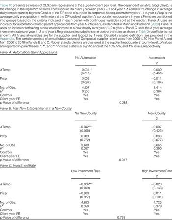
We first analyze the effects of automation using automation-related patent applications, as identified by Mann and Püttmann (Reference Mann and Püttmann2023). As automation technologies increasingly substitute capital for labor, we hypothesize that firms that have applied for an automation-related patent are less sensitive to weather shocks. Panel A of Table 10 presents these results. We find that the coefficient on ∆Temp is negative and statistically significant for firms that have not applied for an automation patent (−0.031) in column 1, but not for firms that have applied in column 2.Footnote 10

TABLE 10 Long description
The table is divided into three panels, each with two columns of data and a final row for the p-Value of difference.
Panel A. Automation Patent Applications:
* Columns: 1 No Automation, 2 Automation.
* Delta Temp: -0.031** (0.019) for column 1; -0.009 (0.499) for column 2.
* Prcp: 0.003 (0.697) for column 1; -0.011 (0.184) for column 2.
* Number of Observations: 4,507 for column 1; 3,414 for column 2.
* R super 2: 0.355 for column 1; 0.364 for column 2.
* Controls and Client-year F E: Yes for both.
* p-Value of difference: 0.288.
Panel B. Has New Establishments in a New County:
* Columns: 1 No New County, 2 New County.
* Delta Temp: -0.042*** (0.005) for column 1; -0.007 (0.423) for column 2.
* Prcp: 0.003 (0.772) for column 1; 0.003 (0.677) for column 2.
* Number of Observations: 3,680 for column 1; 5,665 for column 2.
* R super 2: 0.367 for column 1; 0.390 for column 2.
* Controls and Client-year F E: Yes for both.
* p-Value of difference: 0.047.
Panel C. Investment Rate:
* Columns: 1 Low Investment Rate, 2 High Investment Rate.
* Delta Temp: -0.026*** (0.009) for column 1; -0.020 (0.143) for column 2.
* Prcp: -0.000 (0.977) for column 1; 0.011 (0.101) for column 2.
* Number of Observations: 4,663 for column 1; 4,725 for column 2.
* R super 2: 0.350 for column 1; 0.379 for column 2.
* Controls and Client-year F E: Yes for both.
* p-Value of difference: 0.738.
In Panel B of Table 10, we examine the role of geographic diversification. As reported in Table 8, firms operating in a greater number of counties are less affected by increases in temperature. Building on this finding, we hypothesize that firms that have not diversified their operations geographically (within the past 3 years) will be more vulnerable to temperature shocks. Consistent with this hypothesis, our results show that the coefficient on ∆Temp is negative and statistically significant only for firms that have not expanded operations into a new county (−0.042) in column 1, whereas it is not statistically significant for firms with geographically diversified operations (see column 2).
In Panel C of Table 10, we explore the role of investment. We hypothesize that firms with lower investment rates (measured as the ratio of capital expenditures to lagged property, plant, and equipment) are more affected by temperature shocks, as they are less likely to be transitioning toward a more capital-intensive business model. To test this, we split the sample at the median value of the average investment rate over the past 3 years. We find that the coefficient on ∆Temp is negative and statistically significant only for firms with below-median investment rates (−0.026) in column 1.
B. The Role of Operational and Financial Constraints on Adaptation
Our evidence suggests that these adaptive strategies are effective in mitigating the negative effects of temperature shocks. As Mendelsohn (Reference Mendelsohn2000) argues, firms are likely to undertake substantial adaptation to climate change when the benefits outweigh the costs. However, significant barriers may hinder the implementation of such strategies (e.g., Adger, Agrawala, Mirza, Conde, O’Brien, Pilhin, Pulwarty, Smit, and Takahashi (Reference Adger, Agrawala, Mirza, Conde, O’Brien, Pulhin, Pulwarty, Smit, Takahashi, Parry, Canziani, Palutikof, van der Linden and Hanson2007), Moser and Ekstrom (Reference Moser and Ekstrom2010), Berkhout (Reference Berkhout2012), Biesbroek et al. (Reference Biesbroek, Klostermann, Termeer and Kabat2013)). In light of this, we further examine the role of operational and financial constraints in shaping firms’ adaptive capacity.
We focus on the application of automation patents, as it reflects a shift away from heat-sensitive labor. Because patent applications are firm-level outcomes, the following analyses are conducted at the firm-year level, restricting the sample to suppliers within the client–supplier data set. The dependent variable is an indicator for automation patent applications, which equals 1 if a firm files an automation-related patent application between years t and t + 2. We examine effects up to 2 years ahead to account for potential delays in converting innovation into patent applications.
Table 11 presents the estimates based on sample splits according to financial constraints (proxied by credit rating) and operational constraints (proxied by firm size). In Panel A, we report results for financially or operationally unconstrained firms. Columns 1–3 report that firms that have a credit rating are more likely to apply for an automation patent. The coefficient on ∆Temp ranges from 0.024 to 0.033 and is statistically significant at each horizon. Columns 4–6 report that larger firms (those more likely to have greater operational flexibility) are more likely to apply for automation patents. Although the effects are not statistically significant at conventional levels, the magnitude of the coefficients increases with the time horizon.

TABLE 11 Long description
The table is divided into two panels.
Panel A: Low Operational and Financial Constraints.
This panel includes columns 1 through 3 for Rated firms and columns 4 through 6 for High Assets firms across time horizons t, t plus 1, and t plus 2.
* Delta Temp: For Rated firms, coefficients are 0.024 (p equals 0.073), 0.033 (p equals 0.013), and 0.031 (p equals 0.015). For High Assets, coefficients are 0.006, 0.008, and 0.009, all statistically insignificant.
* Prcp: Coefficients range from 0.003 to 0.006 for Rated and negative 0.017 to negative 0.014 for High Assets, all insignificant.
* Statistics: Number of observations is 1,762 for Rated and 5,821 for High Assets. R-squared values range from 0.458 to 0.505.
Panel B: High Operational and Financial Constraints.
This panel includes columns 1 through 3 for Unrated firms and columns 4 through 6 for Low Assets firms.
* Delta Temp sub t: Coefficients are near zero or slightly negative (e.g., negative 0.004 in column 6) and statistically insignificant across all columns.
* Prcp: Shows a consistent negative correlation with coefficients around negative 0.032 to negative 0.033, all significant at the 1 percent level (p-values between 0.004 and 0.008).
* Statistics: Number of observations is 10,515 for Unrated and 6,448 for Low Assets. R-squared values range from 0.257 to 0.372.
Both panels include Industry-year F E (Fixed Effects) and indicate that regressions are clustered at the supplier headquarters county level.
In Panel B of Table 11, we report results for financially or operationally constrained firms. We find no evidence that such firms—specifically, those that are unrated (columns 1–3) or are smaller in size (columns 4–6)—are more likely to apply for an automation-related patent.
In short, the evidence suggests that less constrained firms are more likely to adapt to increases in local average temperature, whereas more constrained firms are not. Combined with our findings on the underlying economic mechanisms, this indicates that constrained firms are not only more adversely affected by temperature shocks but are also less likely to implement adaptive strategies to mitigate these effects. From a public policy perspective, this highlights the importance of targeting support toward financially and operationally constrained firms, which may lack the capacity to adapt independently (Fankhauser and Soare (Reference Fankhauser and Soare2013)).
VI. Discussion and Robustness
In this section, we show extensions and robustness checks of our primary findings and discuss the interpretation of our results. The Supplementary Material presents these results.
A. Aggregate Effects: Establishment- and Firm-Level Outcomes
Table 12 reports the estimates of establishment-level and firm-level regressions of sales and productivity. Panel A reports establishment-level results. The dependent variable is the change in the logarithm of establishment-level sales in columns 1 and 2 and the change in the establishment sales-to-establishment employee ratio in columns 3 and 4. The main independent variable is the change in local temperature at the ZIP code level. Because pair-level sales data are not available at the establishment level, we cannot include client-by-year fixed effects and therefore do not control for firm-specific demand. We find that temperature shocks do not significantly affect establishment-level sales or productivity.

TABLE 12 Long description
The table is divided into three main sections.
Panel A: Establishment-Level Results.
* Dependent variables: Delta log(Sale super Est.) in columns 1 and 2, and Delta (Sale super Est. all over Employees super Est.) in columns 3 and 4.
* Delta Temp super Est. coefficients range from -0.001 to -0.142, all statistically insignificant.
* Prcp super Est. shows significant negative effects on sales (-0.001) and significant positive effects on sales-per-employee (0.180) in some specifications.
* log(Emp super Est.) has significant negative coefficients of -0.016 and -6.253.
* Observations: 548,078 for sales and 512,852 for sales-per-employee.
Panel B1: Firm-Level Results for a Sample of Suppliers.
* Dependent variables: Delta log(Sales) (cols 1-2), Delta (Sales all over Employees) (cols 3-4), Delta (E B I T all over Assets) (cols 5-6), and Delta (Net Income all over Assets) (cols 7-8).
* Delta Temp and Prcp coefficients are mostly statistically insignificant across all financial metrics.
* Prcp shows a significant negative effect on Delta (Net Income all over Assets) in column 7 (-0.002).
* Observations: Approximately 14,000 to 14,700.
Panel B2: Firm-Level Results for a Sample of Compustat Firms.
* Same dependent variables as Panel B1.
* Prcp shows a significant negative effect on Delta log(Sales) in column 1 (-0.006) and a significant positive effect on Delta (Sales all over Employees) in column 4 (1.555).
* Prcp shows a highly significant negative effect on Delta (Net Income all over Assets) in column 7 (-0.002).
* Observations: Approximately 30,700 to 32,500.
All panels include Firm-year or Industry-year Fixed Effects (F E) and control variables where indicated.
Panel B of Table 12 reports firm-level results using a sample of U.S. firms drawn from the Compustat Industrial Annual database over the 2000–2018 period. We exclude financial firms (SIC codes 6000–6999) and public administration firms (SIC codes 9100–9729). Panel B1 reports results for the sample of U.S. supplier firms in our client–supplier pair-level data. Panel B2 reports results for the broader Compustat sample, without restricting attention to suppliers in the pair-level data, and therefore includes both consumer-facing and smaller firms. The dependent variables are the change in log sales, the change in sales per employee, the change in EBIT to assets (return on assets), and the change in net income to assets. The main explanatory variable is the change in average local temperature at the firm’s headquarters level. As in establishment-level tests, we are unable to include client-by-year fixed effects to control for firm-specific demand. We find that temperature shocks do not significantly affect firm-level sales, productivity, or profitability. Our results are consistent with Addoum et al. (Reference Addoum, Ng and Ortiz-Bobea2020), who find no evidence that temperature shocks affect firm performance using establishment-level or firm-level data.
Firm-level regressions need not align in sign with our supplier–client specifications for both econometric and economic reasons. Econometrically, our identification strategy estimates whether a shocked supplier sells less relative to other suppliers of the same client, not whether its absolute sales increase or decrease. Aggregating to the firm level requires the strong assumption that nonshocked suppliers’ sales to the same client are unchanged, an assumption unlikely to hold when client demand is heterogeneous. Economically, suppliers facing temperature-induced supply constraints may partially offset disruptions through internal reallocation, shifting production across plants, clients, or product lines toward higher-demand or higher-margin opportunities. Consistent with this interpretation, we find no significant effect of temperature on aggregate firm-level sales, productivity, or profitability. Moreover, geographically diversified firms show greater resilience (Table 8), suggesting that multiestablishment firms can redirect production toward less-affected regions. Although our results suggest that demand-side variation contributes to attenuating the firm-level supply effect, we do not have direct evidence on the sign or magnitude of demand responses to temperature shocks. Reconciling aggregate mixed findings requires additional identification of the demand channel, which is beyond the scope of this article.
B. Importance of Economic Mechanisms
We find evidence consistent with several economic mechanisms: the labor productivity and supply channel, the financial constraints channel, the operational flexibility channel, the switching costs channel, and the adaptation channel. Because these mechanisms are not mutually exclusive and the estimated effects are similar across proxies, our results suggest that all of them contribute to explaining how local temperature affects firm sales. Figure IA.1 in the Supplementary Material summarizes the upper and lower bounds of the effect sizes and their statistical significance for each mechanism. The estimated effects of ∆Temp are negative across all five channels and are generally larger for the subsamples expected to be more vulnerable, consistent with labor productivity, financial constraints, operational flexibility, switching costs, and adaptation each playing a role in shaping the sales response to temperature changes.
C. External Validity
We rely on supplier–client data to implement our identification strategy, which restricts the analysis to business-to-business transactions. Although such transactions account for a large share of economic activity, it remains unclear whether our findings generalize to firms outside this setting. Broader firm-level data could, in principle, help address this question, but such data do not allow us to separately identify demand- and supply-side effects. To nonetheless assess external validity, we reweight our sample to better match the broader firm population. Table IA.1 in the Supplementary Material reruns the client–supplier sales growth regressions from Table 2 using inverse probability weights based on total sales within each 2-digit SIC industry. The estimated coefficients on temperature shocks are similar in magnitude to those in Table 2, ranging from −1.9% to −2.7%.
In addition, our identification strategy relies on temperature variation within the sample of suppliers selling to the same client in 1 year. This excludes suppliers selling to only a single client in a given year. However, this exclusion is likely to have a limited impact as the restriction reduces the sample from 1,774 to 1,405 unique suppliers.
D. Robustness
We run additional tests to evaluate the robustness of our results to some of the measurement and estimation choices made for our baseline tests.
Table IA.2 in the Supplementary Material reports the results when we use weather variables at the county level rather than at the ZIP code level. The magnitudes of the coefficients on the change in temperature are similar to those in Table 2, ranging from −1.8% to −3.0%.
Table IA.3 in the Supplementary Material reports the results for the subsample in which the sum of reported firm sales accounts for at least 32% of total sales, corresponding to the median level of supplier sales coverage in our data. This test addresses concerns that the estimated effects on firm sales may be driven by suppliers with limited coverage of interfirm transactions. Although the coefficients on changes in temperature are statistically weaker, their magnitudes remain economically meaningful, ranging from −2.0% to −3.7% when client-by-year fixed effects are included.
Climate shocks are more likely to simultaneously affect the ability of firms to supply products and services as well as demand for such products and services when clients are in the same geographical areas as their suppliers (Ellison and Glaeser (Reference Ellison and Glaeser1997)), as they might be affected by the same weather shocks. In our sample, 84% (87%) of the clients have at least one of their suppliers with an establishment located in the same county (state) as one of the client’s establishments. In Table IA.4 in the Supplementary Material, we restrict the sample to relationships where a client has at least one supplier with an establishment in the same state (Panel A) or county (Panel B) as one of the client’s establishments. The results in Table IA.4 in the Supplementary Material are similar to those in Table 2, although coefficients are estimated with less precision in Panel B.
In Table IA.5 in the Supplementary Material, we focus on average temperature rather than changes in average temperature. The dependent variable is the logarithm of interfirm sales. The regressions include supplier-by-client fixed effects, so we effectively use deviations relative to the mean to estimate the regressions. The results are overall consistent with the notion that when suppliers experience higher temperatures, there is a negative impact on sales compared with other suppliers of the same client in the same year. The estimates are larger in magnitude than those in Table 2.
In Table IA.6 in the Supplementary Material, we examine the role of seasonal variation by focusing on temperature changes during the summer rather than over the full year. The results are qualitatively consistent with our baseline estimates, although they are not statistically significant. This likely reflects the annual frequency of our client–supplier sales data and the resulting limited statistical power.
Table IA.7 in the Supplementary Material reports the results with the change in precipitation as a control variable. In this test, we address the potential concern that instead of controlling for the level of precipitation, we should control for the change in precipitation. The coefficients on the change in precipitation are not statistically different from zero. The magnitudes of the coefficients on the change in temperature are similar to those in Table 2, ranging from −1.8% to −2.7%.
Table IA.8 in the Supplementary Material reports results using alternative standard-error specifications: clustering at the ZIP code level (Panel A), clustering at the firm level (Panel B), and spatially adjusted standard errors as in Colella, Lalive, Sakalli, and Thoenig (Reference Colella, Lalive, Sakalli and Thoenig2020) (Panel C), which address the potential concern that weather variables are spatially correlated at a broader scale (Hsiang (Reference Hsiang2016)). The ∆Temp coefficient remains statistically significant across all specifications.
Our baseline results in Table 2 are estimated using supplier–client relationships that persist for at least 2 consecutive years, because changes in interfirm sales are observed only for continuing relationships. The estimates therefore capture intensive-margin adjustments. In Table IA.9 in the Supplementary Material, we estimate an extensive margin regression based on equation (1) but replace the dependent variable with a dummy that takes a value of 1 if we observe a business transaction in year t – 1 but not in year t, suggesting a termination of the relationship or a significant reduction in transactions between the client and the supplier (below the 10% of sales reporting threshold).
We find that the coefficients are not statistically significant in any of the specifications, suggesting that temperature changes are not likely to lead to the termination (or reduction below the threshold) of supply chain relationships. These results differ from those of Pankratz and Schiller (Reference Pankratz and Schiller2024), who find that heatwaves and natural disasters (floods) can disrupt the global supply chain at the extensive margin. Our findings show that within the United States, changes in average temperature are not as likely to have such a disruptive effect on business relationships. This may be explained by the fact that our sample is a domestic supply-chain network rather than a global one, and clients and suppliers may have stronger business relationships and lower information asymmetries due to their geographical proximity (i.e., they are located in the same county). This finding may also reflect the nature of the weather shocks we study: Changes in average temperature are less severe than the extreme weather events analyzed by Pankratz and Schiller (Reference Pankratz and Schiller2024) and may therefore cause less disruption to supply chain relationships.
Table IA.10 in the Supplementary Material provides additional evidence on the financial constraints channel. We show that these results are driven by more financially constrained firms, as indicated by higher WW, KZ (as constructed in Lamont, Polk, and Saá-Requejo (Reference Lamont, Polk and Saá-Requejo2001)), and SA indices, and a higher proportion of long-term debt maturing within 1 year.
Table IA.11 in the Supplementary Material provides additional evidence on the switching-cost channel. We test the hypothesis that temperature shocks have stronger effects on supplier firms that are more easily replaceable (i.e., those facing lower switching costs). In particular, we hypothesize that suppliers whose clients have greater international exposure are more substitutable, as such clients are likely to have access to a broader set of alternative suppliers and more flexible sourcing options. Consistent with this hypothesis, we find larger effects for suppliers with low patent citations, low interfirm sales share, low market share, fewer clients over the sample period, and whose clients have greater international exposure.
VII. Conclusion
This article studies the effects of changes in average temperature in the real economy by exploiting variation in production networks. We compare sales of intermediate goods across suppliers that trade with the same client but are exposed to different changes in temperature, which allows us to isolate supply-side effects from demand-side effects.
We show that changes in local temperature can have sizable effects on firm sales at the intensive margin. A 1°C increase in average local temperature leads to a negative and significant effect of about 2.5% on annual sales. We interpret these effects as supply-driven, because they originate from the supplier’s exposure to temperature. Sales declines are more pronounced among firms experiencing larger temperature increases and among firms located in cooler regions.
We examine the mechanisms through which changes in local temperature affect firm sales. First, the reduction in sales due to increases in local temperature is primarily driven by firms operating in heat-sensitive industries, manufacturing industries, and labor-intensive firms, suggesting that lower labor supply and productivity are driving our effects. Second, we find that financially unconstrained firms are better able to deal with the adverse effects of increased local temperature and, therefore, face lower temperature-related reductions in sales. This suggests that financial constraints play an essential role in firms’ ability to adapt to climate change. Conglomerates and firms that are geographically diversified also cope better with the effects of climate change as they have more operational flexibility. Finally, input specificity and switching costs are important drivers of the impact of temperature on firm sales. The evidence suggests that suppliers experience a smaller decline in sales when they produce specific inputs or when their clients have higher switching costs.
Overall, our findings suggest that climate change can materially affect firm sales and real economic activity. These results underscore the importance of isolating supply-side channels when designing policy responses to climate change. They also highlight the need to target support toward financially and operationally constrained firms, which may lack the capacity to adapt without external assistance. Credibly identifying the demand-side effects of temperature shocks, and whether they reinforce or offset supply-side losses, remains an important direction for future research.
Appendix. Variable Definitions
- Δlog(Sales):
-
Change in the logarithm of sales from supplier i to client j from year t – 1 to year t. Source: Compustat.
- ∆Temp:
-
Change in the annual average daily mean temperature from year t – 1 to year t, measured in degrees Celsius, at the ZIP code of supplier i’s corporate headquarters. Daily mean temperature is the average of daily maximum and minimum temperatures. Source: Compustat and PRISM.
- ∆Temp Est. emp.-weighted:
-
Change in the annual average establishment employment-weighted daily mean temperature from year t – 1 to year t, measured in degrees Celsius. Daily mean temperature is the average of daily maximum and minimum temperatures. Establishment-level temperature is measured at the ZIP codes of supplier i’s establishments, then aggregated to the firm level using the number of employees in each establishment as weights. Source: Compustat, NETS, and PRISM.
- Temp:
-
Annual average daily mean temperature in year t, measured in degrees Celsius, at the ZIP code of supplier i’s corporate headquarters. Daily mean temperature is the average of daily maximum and minimum temperatures. Source: Compustat and PRISM.
- Temp Est. emp.-weighted:
-
Annual average establishment employment-weighted daily mean temperature in year t, measured in degrees Celsius. Daily mean temperature is the average of daily maximum and minimum temperatures. Establishment-level temperature is measured at the ZIP codes of supplier i’s establishments, then aggregated to the firm level using the number of employees in each establishment as weights. Source: Compustat, NETS, and PRISM.
- Prcp:
-
Annual average daily precipitation in year t, measured in millimeters, at the ZIP code of supplier i’s corporate headquarters. Source: Compustat and PRISM.
- Prcp Est. emp.-weighted:
-
Annual average establishment employment-weighted daily precipitation in year t, measured in millimeters. Establishment-level precipitation is measured at the ZIP codes of supplier i’s establishments, then aggregated to the firm level using the number of employees in each establishment as weights. Source: Compustat, NETS, and PRISM.
- Assets:
-
Total assets in year t – 1. Source: Compustat AT.
- Cash:
-
Cash and cash equivalents in year t – 1, divided by total assets in year t – 1. Source: Compustat CHE/AT.
- Leverage:
-
Total debt in year t – 1, defined as debt in current liabilities plus long-term debt, divided by market value of assets in year t – 1. Source: Compustat (DLC + DLTT)/(DLC + DLTT + CSHO × PRCC_F).
- Tangibility:
-
Net property, plant, and equipment in year t – 1, divided by total assets in year t – 1. Source: Compustat PPENT/AT.
- Tobin’s Q:
-
Market value of assets in year t – 1, defined as total assets plus market value of equity minus book value of equity, divided by total assets in year t – 1. Source: Compustat (AT + CSHO × PRCC_F – [AT – (LT + PSTKL) + TXDITC])/AT.
- Temperature normal:
-
Thirty-year average daily mean temperature, measured in degrees Celsius, at the ZIP code of supplier i’s corporate headquarters from 1981 to 2010. Source: Compustat and PRISM.
- Positive deviation:
-
Annual average positive temperature deviations in year t, measured in degrees Celsius, at the ZIP code of supplier i’s corporate headquarters. For each day, the positive temperature deviation is calculated as the difference between daily mean temperature and monthly temperature normal if the daily mean temperature exceeds the monthly temperature normal, and 0 otherwise. Source: Compustat and PRISM.
- Absolute deviation:
-
Annual average absolute temperature deviations in year t, measured in degrees Celsius, at the ZIP code of supplier i’s corporate headquarters. For each day, the absolute temperature deviation is calculated as the absolute value of the difference between daily mean temperature and monthly temperature normal. Source: Compustat and PRISM.
- Summer temperature (calendar):
-
Seasonal average of daily mean temperatures during meteorological summer (i.e., from June to August) in year t, measured in degrees Celsius, at the ZIP code of supplier i’s corporate headquarters. Source: Compustat and PRISM.
- Summer temperature (average normal):
-
Seasonal average of daily mean temperature during summer, defined as the 3 months with the highest monthly temperature normals, in year t, measured in degrees Celsius, at the ZIP code of supplier i’s corporate headquarters. Source: Compustat and PRISM.
- Cold/windchill:
-
Indicator variable equal to 1 if the county of supplier i’s corporate headquarters has experienced a cold/windchill event that has resulted in at least one fatality in year t, and 0 otherwise. A cold/windchill event is a period of low temperatures or windchill temperatures reaching or exceeding locally/regionally defined advisory conditions. Source: Compustat and NOAA.
- Heavy snow:
-
Indicator variable equal to 1 if the county of supplier i’s corporate headquarters has experienced a heavy snow event that has resulted in at least one fatality in year t, and 0 otherwise. A heavy snow event happens when snow accumulation meets or exceeds locally/regionally defined 12 and/or 24 h warning criteria. Source: Compustat and NOAA.
- Heat:
-
Indicator variable equal to 1 if the county of supplier i’s corporate headquarters has experienced a heat event that has resulted in at least one fatality in year t, and 0 otherwise. A heat event is a period of heat resulting from the combination of high temperatures (above normal) and relative humidity. Source: Compustat and NOAA.
- Hot days:
-
Number of days in year t for which the daily mean temperature exceeds the corresponding monthly temperature normal by at least 5°C at the ZIP code of supplier i’s corporate headquarters. Source: Compustat and PRISM.
- Heavy rain:
-
Indicator variable equal to 1 if the county of supplier i’s corporate headquarters has experienced a heavy rain event that has resulted in at least one fatality in year t, and 0 otherwise. A heavy rain event is an unusually large amount of rain that does not cause a flash flood or flood event but causes damage, for example, roof collapse or other human/economic impact. Source: Compustat and NOAA.
- Flood:
-
Indicator variable equal to 1 if the county of supplier i’s corporate headquarters has experienced a flood event that has resulted in at least one fatality in year t, and 0 otherwise. A flood event is any high flow, overflow, or inundation by water that causes damage. Source: Compustat and NOAA.
- Manufacturing industries:
-
Industries with SIC codes between 2000 and 3999. Source: Compustat.
- Occupational heat exposure:
-
Job zone scores aggregated at 3-digit SIC or 4-digit NAICS levels. Source: Occupational Information Network and Bureau of Labor Statistics’ Occupational Employment and Wage Statistics.
- Labor intensity:
-
Number of employees in year t – 1 divided by total assets in year t – 1. Source: Compustat EMP/AT.
- Credit rating:
-
Indicator variable equal to 1 if supplier i has a credit rating from S&P in year t – 1, and 0 otherwise. Source: Compustat.
- Payout ratio:
-
Payout in year t – 1, defined as the sum of preferred dividends, common dividends, and purchases of common and preferred stocks, divided by income before extraordinary items in year t – 1. Source: Compustat (DVP + DVC + PRSTKC)/IB.
- Financial constraints composite index:
-
Composite financial constraints index in year t – 1, following Bartram et al. (Reference Bartram, Hou and Kim2022). The index is constructed as the sum of indicator variables based on the KZ index, WW index, SA index, size, payout ratio, and credit rating, where each indicator reflects whether the firm is classified as financially constrained according to the respective measure. Source: Compustat.
- Number of counties with establishment:
-
Number of counties where supplier i has at least one establishment. Source: Compustat and NETS.
- HHI establishment sales:
-
Herfindahl–Hirschman Index of establishment-level sales for supplier i in year t – 1, computed as the sum of squared shares of each establishment’s sales in supplier i’s total sales. Source: NETS.
- Standardized goods:
-
Indicator variable equal to 1 if supplier i belongs to an industry that is more likely to sell standardized products as defined in Giannetti et al. (Reference Giannetti, Burkart and Ellingsen2011), and 0 otherwise. Source: Compustat.
- Innovation value:
-
Market-adjusted stock returns on the 3-day window around the patent issue date. Source: Kogan et al. (Reference Kogan, Papanikolaou, Seru and Stoffman2017).
- Duration of supplier–client relationship:
-
Number of years when supplier i has a transaction with client j over the sample period. Source: Compustat.
- Automation patent application:
-
Indicator variable equal to 1 if supplier i has made an automation-related patent application in year t, based on the definition in Mann and Püttmann (Reference Mann and Püttmann2023). Source: Mann and Püttmann (Reference Mann and Püttmann2023).
- Investment rate:
-
Capital expenditures in year t, divided by net property, plant, and equipment in year t – 1. Source: Compustat CAPEX/PPENT.
- Δlog(SalesEst.):
-
Change in the logarithm of sales at establishment e from year t – 1 to year t. Source: NETS.
- ∆(SalesEst. /EmpEst.):
-
Change in the ratio of establishment sales-to-establishment employment from year t – 1 to year t. Source: NETS.
- ∆TempEst.:
-
Change in the annual average daily mean temperature from year t – 1 to year t, measured in degrees Celsius, at the ZIP code of establishment e. Daily mean temperature is the average of daily maximum and minimum temperatures. Source: NETS and PRISM.
- PrcpEst.:
-
Annual average daily precipitation in year t, measured in millimeters, at the ZIP code of establishment e. Source: NETS and PRISM.
- Δlog(Sales):
-
Change in the logarithm of total sales for supplier i from year t – 1 to year t. Source: Compustat.
- Δ(Sales/Employees):
-
Change in the ratio of total sales in year t to total employees in year t – 1. Source: Compustat.
- Δ(EBIT/Assets):
-
Change in the ratio of operating income in year t divided by total assets in year t – 1. Source: Compustat.
- Δ(Net Income/Assets):
-
Change in the ratio of net income in year t to total assets in year t – 1. Source: Compustat.
- log(EmpEst.):
-
Logarithm of employment at establishment e in year t – 1. Source: NETS.
Supplementary Material
To view supplementary material for this article, please visit http://doi.org/10.1017/S002210902610341X.
Funding Statement
Custódio acknowledges financial support from the European Research Council Grant (Project 852677—grow). Ferreira acknowledges financial support from the Fundação para a Ciência e a Tecnologia.