


I. Introduction
Climate-related risks are difficult to assess and process for nonexperts (e.g., due to lack of information, limited attention, or the lack of a model). As a result, regulators may be concerned that households do not correctly account for such risks when choosing in which neighborhood to locate or how much to pay for a home. Risk zoning (e.g., for flood or wildfire) has become a commonly used policy intervention to provide risk information to households and make the risk more salient for homes located inside the risk zone. Risk zoning has the potential to affect the location of housing developments, and thus in turn the economic costs of natural disasters (Rappaport and Sachs (Reference Rappaport and Sachs2003), Kahn (Reference Kahn2005)). For example, an estimated 46 million homes and $9.2 trillion in property value are currently located in the wildland–urban interface and are exposed to wildfire risk in the United States (International Association of Wildland Fire (2013), Radeloff, Helmers, Kramer, Mockrin, Alexandre, Bar-Massada, Butsic, Hawbaker, Martinuzzi, Syphard, and Stewart (Reference Radeloff, Helmers, Kramer, Mockrin, Alexandre, Bar-Massada, Butsic, Hawbaker, Martinuzzi, Syphard and Stewart2018)).
How information about low-probability, high-consequence risks is incorporated into the prices of large, illiquid, widely-held assets is a first-order question in asset pricing. Residential real estate is the largest asset class held by U.S. households and a central component of the financial system through mortgage and insurance markets. A growing share of its value is exposed to climate-related hazard. Understanding whether, and how, households as marginal investors in this market process newly disclosed risk information, and whether they respond to the salience of a discrete risk classification rather than to the underlying continuous risk, has direct implications for housing market price formation, for the spatial reallocation of development relative to risk boundaries, and for the collateral risk borne by mortgage lenders and insurers. Risk rezoning events provide a setting to examine whether the salience of climate-related risk drives household risk-taking and asset prices.
This article estimates the effect of a new climate-related risk zone on residential real estate prices, both at the new zone boundary and further away. Comparing the two estimates separates the effect of risk salience from the effect of risk information.Footnote 1 I exploit California’s 2007 revision of its wildfire risk zones, which required sellers to disclose a home’s risk-zone status to prospective buyers. This disclosure makes wildfire risk more salient for homes inside the newly designated risk zone than for nearby homes just outside the boundary. Throughout, I treat risk salience as discontinuous at the new zone boundary. While some homes are newly assigned to the risk zone, others experience a change in their pre-2007 risk zone level. Using real estate sales transactions for the universe of homes in Southern California, I exploit this policy shift together with the spatial discontinuity in risk salience at the new risk zone boundary. This allows me to identify the effect of risk salience on residential real estate prices.
To identify the effect of the risk zone on residential real estate prices, I rely on three empirical designs. First, a spatial regression discontinuity (RD) design compares homes just inside and just outside the new boundary. I find that the estimated local average treatment effect (LATE) on prices is null. Second, a difference-in-discontinuities (RD-DiD) design compares prices across the boundary before and after the 2007 change: the LATE is again null. Third, a difference-in-differences (DiD) design in the immediate vicinity of the boundary yields a null average treatment effect on the treated (ATT). Under the assumption that mandated disclosure makes the weighting of wildfire risk discontinuous at the boundary, these null results indicate that households do not respond to the increased salience of risk. The estimates are robust to alternative bandwidths, sample selections, covariates, and fixed effects. The null results could instead mean that households ignore wildfire risk entirely. To test this, I estimate the DiD including homes further from the boundary. The ATT is −5.7% in the preferred specification with home and county-by-year fixed effects. Households are attentive to wildfire risk: they update their beliefs in response to the new zone, but not to the salient boundary itself. Despite this price decline for reclassified homes, mortgage loan-to-value ratios show no corresponding adjustment, implying that lenders’ effective collateral exposure grew silently as affected home values fell.
I explore several mechanisms that could explain the coexistence of null LATEs and ATT in the immediate vicinity of the new risk zone boundary and significantly negative ATT on home prices further away. Contrasting these price estimates with high-resolution, objective wildfire risk measures that were not available to households at the time, I find that the actual wildfire risk is continuous in the immediate vicinity of the new risk zone boundary and increases further away, mirroring the price results. These findings suggest that households use the new risk zone to update their risk beliefs and, thus, make their asset pricing decisions consistent with a rational decision-making model.Footnote 2
These findings contribute to the literature on belief formation and asset prices (Brunnermeier, Gollier, and Parker (Reference Brunnermeier, Gollier and Parker2007), Brunnermeier, Farhi, Koijen, Krishnamurthy, Ludvigson, Lustig, Nagel, and Piazzesi (Reference Brunnermeier, Farhi, Koijen, Krishnamurthy, Ludvigson, Lustig, Nagel and Piazzesi2021)) and to the literature on salience (Chetty, Looney, and Kroft (Reference Chetty, Looney and Kroft2009), Bordalo, Gennaioli, and Shleifer (Reference Bordalo, Gennaioli and Shleifer2012), (Reference Bordalo, Gennaioli and Shleifer2013), and Gabaix (Reference Gabaix2014)). In the context of a large and risky asset, I find that households do not respond to the increased salience of risk generated by a policy intervention. This contrasts with documented responses to the salience of prices (e.g., Finkelstein (Reference Finkelstein2009)) and of risk (Célérier and Vallée (Reference Célérier and Vallée2017), Frydman and Wang (Reference Frydman and Wang2020)) involving smaller purchases and contributes to the prior literature on risk salience and real estate prices.
My comparison of LATE and ATT in the immediate vicinity of a boundary contrasts with the quasi-experimental literature that examines how climate-related risk salience affects residential real estate prices using ATTs. For instance, Giglio, Maggiori, Rao, Stroebel, and Weber (Reference Giglio, Maggiori, Rao, Stroebel and Weber2021b) examine the effect of future sea-level-rise risk salience on home prices using variation in a “climate attention index” accounting for the frequency of climate-related language in for-sale listings. This setting does not lend itself to an RD design because there is no natural boundary where the salience of risk might be discontinuous, in contrast to my setting with a spatial risk salience discontinuity at the new risk zone boundary. A related strand of literature examines the effect of future sea-level-rise risk on home prices (e.g., Bernstein, Gustafson, and Lewis (Reference Bernstein, Gustafson and Lewis2019), Baldauf, Garlappi, and Yannelis (Reference Baldauf, Garlappi and Yannelis2020), and Murfin and Spiegel (Reference Murfin and Spiegel2020)). In contrast to these studies exploiting variation in risk, my article focuses on variation in the salience of risk at the new risk zone boundary, holding risk constant. More recently, Letta and Nocito (Reference Letta and Nocito2025) document that a sharp rise in the salience of volcanic risk near Naples, absent new physical damage, moved local real estate prices, illustrating that salience can be quantitatively important for infrequently traded assets when the signal is sufficiently large. The literature on climate risk capitalization in housing has grown rapidly; see Contat, Hopkins, Mejia, and Suandi (Reference Contat, Hopkins, Mejia and Suandi2024) for a recent survey and Giglio, Kelly, and Stroebel (Reference Giglio, Kelly and Stroebel2021a) for a broader review of climate finance. Other studies use changes in risk maps to estimate ATTs, such as flood zone maps (e.g., Gibson and Mullins (Reference Gibson and Mullins2020), Hino and Burke (Reference Hino and Burke2021))Footnote 3 or wildfire risk ratings (Donovan, Champ, and Butry (Reference Donovan, Champ and Butry2007)).Footnote 4 Closely related to this article, Ma, Walls, Wibbenmeyer, and Lennon (Reference Ma, Walls, Wibbenmeyer and Lennon2024) use a boundary discontinuity design around California wildfire risk zones and find a 4.3% price discount at boundaries. Because their design is a pooled cross section of sales from 2015 to 2022, their estimate reflects the value differential between homes that have always been inside the zone and homes that have always been outside it, rather than an effect of being newly reclassified.Footnote 5
The article relates to the literature examining how risk salience from a recent natural disaster affects decision-makers’ choices. For example, recent natural disasters have been shown to affect real estate prices in high-risk areas not directly hit by the event, for example, for flooding and hurricanes (e.g., Hallstrom and Smith (Reference Hallstrom and Smith2005), Muller and Hopkins (Reference Muller and Hopkins2019), and Addoum, Eichholtz, Steiner, and Yönder (Reference Addoum, Eichholtz, Steiner and Yönder2024))Footnote 6 and wildfires (e.g., McCoy and Walsh (Reference McCoy and Walsh2018)). Dessaint and Matray (Reference Dessaint and Matray2017) find that corporate managers increase their cash holdings after a recent hurricane. Gallagher (Reference Gallagher2014) shows that households temporarily increase flood insurance purchases after a flood event is reported in their television media market. Choi, Diffenbaugh, and Burke (Reference Choi, Diffenbaugh and Burke2024) similarly find that flood exposure raises insurance adoption, but effects decay within 5 years. Although a recent natural disaster does not change the risk per se, it may affect decision-makers’ risk beliefs, for example, due to recency effects (Agarwal, Driscoll, Gabaix, and Laibson (Reference Agarwal, Driscoll, Gabaix and Laibson2008), Malmendier (Reference Malmendier2021)).
Section II provides background on the risk zones. Section III describes the data, Section IV the empirical strategy, and Section V the results. Section VI discusses mechanisms, and Section VII concludes.
II. Background on the Fire Risk Zones and Wildfire Risk
A. Policy Motivation
California adopted its first wildfire risk zones in 1985. In November 2007, the state adopted new zones under Title 14 to incorporate improved fire science, data, and mapping techniques (CAL FIRE (2022)). The 2007 zones have two objectives: to inform residents about fire hazard in their area and to impose fire-safe building standards on new construction. A later map revision, released in November 2022, is beyond the scope of this study.
B. Risk Zone Design
The wildfire risk zones, referred to by the State of California as Fire Hazard Severity Zones or FHSZs, are produced by the California Department of Forestry and Fire Protection (CAL FIRE; see CAL FIRE (2022) for details). CAL FIRE’s model predicts potential fire behavior and the probability of an area burning, using “the best available science and data at the time” (CAL FIRE (2022)). Each area receives a hazard score based on continuous inputs: existing and potential fuel (natural vegetation), terrain characteristics, and typical fire weather. There are three zone levels: moderate, high, and very high.
C. Risk Zone Implementation
The 2007 risk zone revises and, in most places, marginally expands the pre-existing 1985 risk zone, with small contractions in some areas. Typically, the 2007 change in the zone boundary does not exceed a couple of kilometers, as illustrated in Sections A.2 and A.3 of the Supplementary Material. Importantly, because the zone represents overall hazard rates, homeowners cannot take private risk-mitigating actions to affect their zone assignment. Sellers are mandated by law to disclose to prospective buyers at the time of sale whether their home lies inside a risk zone and, if so, which one. In practice, after Jan. 1, 2008, being located inside a risk zone (no matter the level) comes with permit requirements for new buildings, or extensions or remodeling of the exterior made to existing buildings, that must comply with California Building Code Chapter 7a. The implication is that roofs, exterior walls, and decks should use ignition-resistant materials.
The zones were designed not to raise insurance premiums. California regulation prohibits insurers from pricing on risk-zone status, and insurance companies use proprietary, fine-resolution probabilistic risk models that supersede the coarse hazard classes in the zones.Footnote 7 Nevertheless, I test empirically in Section E of the Supplementary Material and fail to find an effect of the new risk zone on insurance premium quotes or on mortgages as measured by rate spread, loan-to-value, and mortgage terms.
D. Wildfire Risk Measures
The first publicly available fine-resolution wildfire risk measures for California were published in 2020 by the U.S. Forest Service (Scott, Gilbertson-Day, Moran, Dillon, Short, and Vogler (Reference Scott, Gilbertson-Day, Moran, Dillon, Short and Vogler2020)). They reflect the wildfire risk that prevailed circa 2014 for every 30 m
$ \times $
 30 m pixel in the landscape. I assume that this wildfire risk approximates the overall wildfire risk in my 2000–2015 time period. The two risk measures of interest are i) the wildfire or burn probability, which represents the annual probability of a wildfire burning in a specific location, and ii) the fire risk to homes or risk to potential structures (RPS), which for every pixel provides the probability that a home would burn if a home existed on that pixel. I convert these annual risk measures into the probability of at least one risky event occurring in the next 30 years to better match the time horizon associated with real estate purchases.
III. Data
The data sets include home sales transactions, the wildfire risk zone, high-resolution fire risk measures, and neighborhood characteristics. This section describes the main variables, while Section A of the Supplementary Material contains details of the data cleaning, additional data sources to test for sorting and alternative mechanisms, the summary statistics, and illustrations of the spatial distribution of the homes, risk zones, and fire risk measures.
A. Home Sales Transactions
The home sales transactions were obtained from CoreLogic and cover all single-family sales (excluding mobile homes) between January 2000 and December 2015 in ZIP codes most likely to be affected by wildfire risk across seven counties in the Los Angeles and San Diego Basins, namely, Santa Barbara, Los Angeles, Orange, Ventura, Riverside, San Bernardino, and San Diego. The key variables are the sale price and sale date, address, and home characteristics such as size, age, number of bedrooms and bathrooms, and presence of a swimming pool. Every home is geocoded and matched to a series of spatial layers, including wildfire perimeters, topography, and fire risk measures. Homes are linked to the American Community Survey (ACS) to obtain demographics at the census tract level.
Starting with a data set of 2,187,007 unique properties, I focus on owner-occupied properties and arm’s-length transactions. All prices are deflated using the Consumer Price Index from the U.S. Bureau of Labor Statistics. In addition, to focus on the sole effect of the new risk zone absent any realization of wildfire risk in the vicinity, I drop a small number of homes located within 10 km of a wildfire perimeter that burned within 3 years prior to a sale.
B. Location Inside the Fire Risk Zone
The geocoded homes are mapped into both the old (pre-2007) and new (post-2007) fire risk zones obtained from CAL FIRE. For each risk zone, there exist three levels: moderate, high, and very high. For each home inside the new risk zone, I calculate its distance to the new risk zone boundaries. For example, if a home is located inside the high-risk zone, I calculate the distance to the moderate and to the very high-risk zone boundaries. For each home outside the new risk zone, I calculate its distance to the moderate risk zone boundary. The moderate and high-risk zones are relatively thin, while the very high-risk zone is vast as it extends into the wilderness. In my sample, the median (max) width for the new moderate zone is 1.1 km (5.8 km), and for the new high-risk zone it is 540 m (4.1 km).
C. Definition of the Treatment and Control Homes
Throughout the article, I define as control homes those that do not change risk zone level in 2007, while I define as treatment homes those that experience a one-level increase in their risk zone.Footnote 8 For example, a treatment home is located inside the moderate risk zone prior to 2007 and inside the high-risk zone after 2007. I observe its sale either before or after 2007, or in some cases both before and after 2007. In addition, to improve the comparability of treated and control homes, I restrict observations i) to come from census tracts that feature both control and treatment homes (this restriction is relaxed in Section C of the Supplementary Material and results are quantitatively similar), and ii) to be located within 1 km of the new risk zone boundary.
Few treatment homes move from outside the zone into the moderate zone, so I drop this treatment from the main analysis. I pool the two remaining one-level increases (moderate to high, and high to very high) into a generic one-level increase. Sections A.3 and D of the Supplementary Material report observation counts and DiD estimates for each individual increase. Results are similar.
IV. Empirical Strategy
This section lays out the three empirical models. The first two identify the effect of risk salience at the new zone boundary on home prices; the third identifies the effect of the risk information contained in the new zone.
A. Regression Discontinuity Design
I implement a spatial RD design to estimate the LATE of being located inside a riskier wildfire zone on home prices. The spatial RD model is shown in equation (1):

where the dependent variable is the natural logarithm of home
$ i $
 ’s sale price. The running variable
$ {x}_i $
 measures the distance of home
$ i $
 to the new risk zone boundary, with cutoff
$ \overline{x}=0 $
 . The dummy variable
$ Z $
 takes value 1 for treated homes (
$ {x}_i\ge 0 $
 ) and 0 for control homes (
$ {x}_i<0 $
 ). Treated homes are always located inside a zone that is one level higher after the 2007 policy change than the control homes, which do not change risk zone level.
$ {g}_0\left({x}_i\right) $
 and
$ {g}_1\left({x}_i\right) $
 are two continuous polynomials of order
$ p $
 . The coefficient
$ \tau $
 is the treatment effect (i.e., the change in
$ \ln {p}_i $
 at the cutoff).
The bandwidth is selected by the MSE-optimal, data-driven procedure of Calonico, Cattaneo, and Titiunik (Reference Calonico, Cattaneo and Titiunik2014a), (Reference Calonico, Cattaneo and Titiunik2014b). All specifications employ a triangular kernel; the main specification uses a local linear polynomial (Gelman and Imbens (Reference Gelman and Imbens2019)). Following Cattaneo, Titiunik, and Vazquez-Bare (Reference Cattaneo, Titiunik, Vazquez-Bare, Curini and Franzese2020b), throughout the article I report conventional point estimates, robust bias-corrected standard errors and confidence intervals, and robust
$ p $
 -values. Standard errors are computed using the heteroscedasticity-robust nearest-neighbor variance estimator with a minimum of three neighbors.Footnote
9 I estimate equation (1) for homes that sell after the new risk zone implementation, both without and with covariates, as including covariates can improve estimation efficiency. Covariates for the RD include: home age, size, number of bedrooms, presence of a swimming pool, distances to the nearest primary road and to the nearest national forest, and location inside the wildland–urban interface.
The strength of the RD design is to compare homes that are located as close as possible to the new risk zone boundary to ensure the treated and control homes are as similar as possible and only differ with respect to their risk zone assignment. The design requires that home characteristics, observed and unobserved, do not change discontinuously at the cutoff. Section B.1 of the Supplementary Material shows that covariates are continuous around the cutoff: re-estimating equation (1) with each covariate as the dependent variable yields no discontinuity.
The RD design also requires that homeowners cannot manipulate their assignment at the cutoff. The risk zones are designed to reflect hazard rates over broad areas such that a particular homeowner cannot take risk-mitigating actions (e.g., clearing vegetation around the home) to affect their assignment to the risk zone. Still, I formally test for manipulation of risk zone assignment at the cutoff in Section B.1 of the Supplementary Material. Using the testing procedure from Cattaneo, Jansson, and Ma (Reference Cattaneo, Jansson and Ma2020a), I fail to reject the null hypothesis of continuity of the density of the running variable (
$ p>0.1 $
 ).
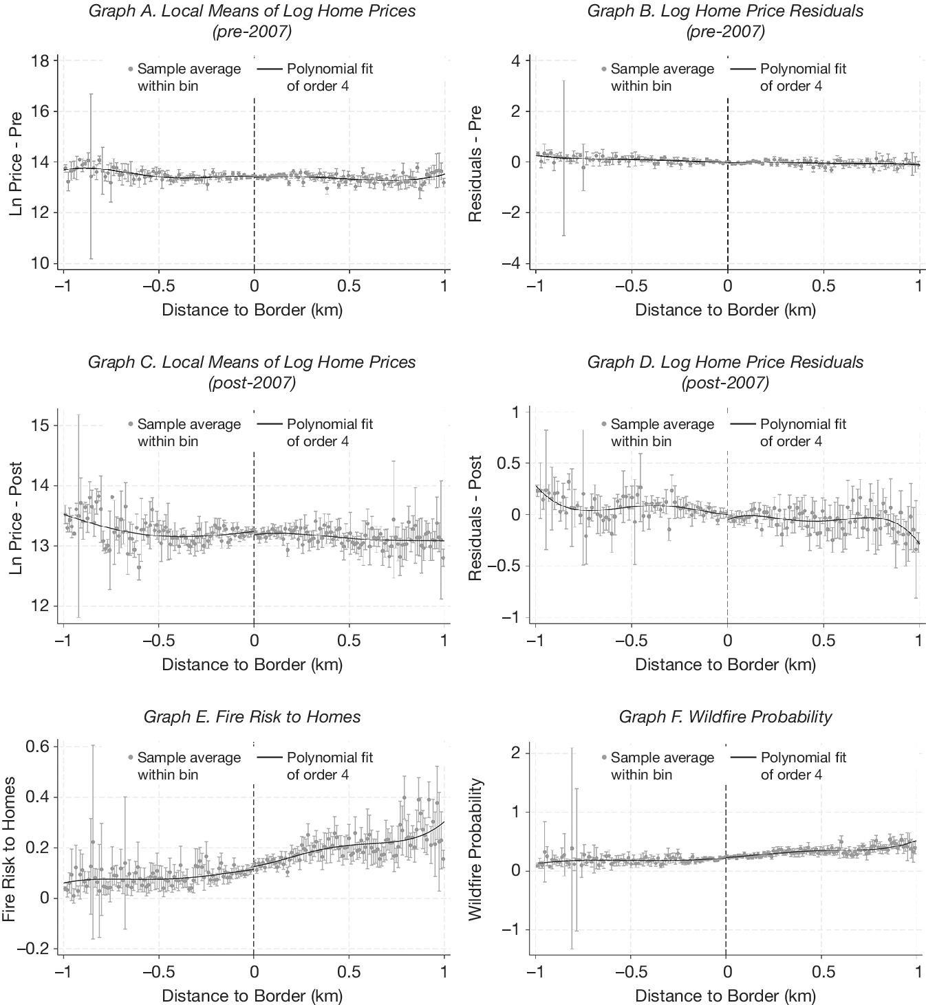
Graphs A and C of Figure 1 depict the local logarithm price means of the treated (right) and control (left) homes, while Graphs B and D show the residuals of logarithm prices on covariates in the pre-treatment period (Graphs A and B) and post-treatment period (Graphs C and D). Fitting a polynomial of order 4 does not indicate evidence of a discontinuity at the new risk zone boundary in either the pre- or post-treatment period. Graphs E and F illustrate the fire risk to homes and wildfire probability over 30 years, respectively. The risk increases smoothly from left (control) to right (treated homes).
Graphs A–D of Figure 1 show logarithm home prices by distance to the 2007 risk zone boundary, before (A–B) and after (C–D) the rezoning: local means in (A) and (C), and residuals from a regression of logarithm prices on covariates (age, house size, number of bedrooms, swimming pool dummy, distances to nearest primary road and national forest, and wildland–urban interface dummy) in (B) and (D). Graphs E and F show the fire risk to homes and the wildfire probability. Homes to the right of the cutoff are inside a risk zone one level higher than homes to the left. The number of bins is data-driven (Calonico et al. (Reference Calonico, Cattaneo and Titiunik2015)). Vertical bars denote 90% confidence intervals. A polynomial of degree four is fitted on each side. Observations are restricted to census tracts featuring both control and treatment homes.

FIGURE 1 Long description
A multi-panel set of six line graphs labeled A through F. All graphs share a common x-axis titled Distance to Border in km, ranging from negative 1 to 1, with a vertical dashed line at 0 representing the risk zone boundary.
* Graph A: Local Means of Log Home Prices pre-2007. The y-axis is Ln Price minus Pre, ranging from 10 to 18. Data points and a fourth-order polynomial fit show a relatively flat trend around 13.5 across the boundary.
* Graph B: Log Home Price Residuals pre-2007. The y-axis is Residuals minus Pre, ranging from negative 4 to 4. The data is tightly clustered around 0 with a flat polynomial fit.
* Graph C: Local Means of Log Home Prices post-2007. The y-axis is Ln Price minus Post, ranging from 12 to 15. The polynomial fit shows a slight downward slope from negative 1 to 0, then remains flat after the boundary.
* Graph D: Log Home Price Residuals post-2007. The y-axis is Residuals minus Post, ranging from negative 1 to 1. The polynomial fit shows a slight dip and recovery around the boundary.
* Graph E: Fire Risk to Homes. The y-axis ranges from negative 0.2 to 0.6. The polynomial fit shows a steady increase in fire risk as distance increases from negative 1 to 1, crossing the boundary at approximately 0.1.
* Graph F: Wildfire Probability. The y-axis ranges from negative 1 to 2. The polynomial fit shows a gradual upward trend from 0.1 at negative 1 to approximately 0.5 at 1.
Each graph includes gray dots for sample average within bin, vertical gray bars for 90 percent confidence intervals, and a solid black line for the polynomial fit of order 4.
Because one cannot test formally that no unobservables are changing discontinuously at the new risk zone boundary, this motivates the use of a second design leveraging homes that sold before and after the new 2007 risk zone implementation.Footnote 10
B. Difference-in-Discontinuities Design
The difference-in-discontinuities (RD-DiD) model estimates a continuous polynomial on each side of the cutoff (
$ \overline{x}=0 $
 ) both before and after the policy change, as depicted in equation (2):

where
$ t $
 denotes time and
$ {Post}_t $
 is a dummy taking value 1 in the period following the 2007 change in risk zoning. The treatment effect,
$ \tau $
 , captures the change in
$ \ln {p}_{it} $
 at the cutoff, comparing before and after the policy change. In the main specification, the polynomial
$ {g}_j\left({x}_{it}\right) $
 , where
$ j\in \left[0,3\right] $
 , is of degree one.
C. Difference-in-Differences Design
I estimate an average treatment effect on the treated (ATT) comparing the prices of homes that experience an increase in their risk zone level with those of homes that remain in the same risk zone. The DiD model is depicted in equation (3):

where the dependent variable is the natural logarithm of home
$ i $
 ’s sale price at time
$ t $
 . The treatment group,
$ {Treat}_i $
 , is defined as all homes that are located inside a zone that is one level higher than that prior to the 2007 risk zone implementation. The control group is defined as homes that remain inside the same risk zone after the new 2007 risk zone implementation.
$ {Post}_t $
 is a dummy variable taking value 1 following the 2007 change in risk zoning. The coefficient
$ {\beta}_{DiD} $
 is the ATT. In the simplest specification,
$ {\mathbf{X}}_i $
 denotes home and neighborhood covariates, while the preferred specification features home fixed effects
$ {\lambda}_i $
 to most flexibly control for time-invariant unobservables, such as home and neighborhood quality. Covariates in the DiD include home age and age squared, home size and home size squared, number of bedrooms, number of baths, swimming pool dummy, elevation, slope, dummy for location inside the wildland–urban interface, distances to nearest primary road, to nearest national forest, and to nearest state or local park. To control for temporal shocks (e.g., macro-level housing shocks) and possible heterogeneity in temporal shocks across the region,
$ {\mu}_{gt} $
 denotes year and quarter fixed effects or, more flexibly, county-by-year and quarter fixed effects.
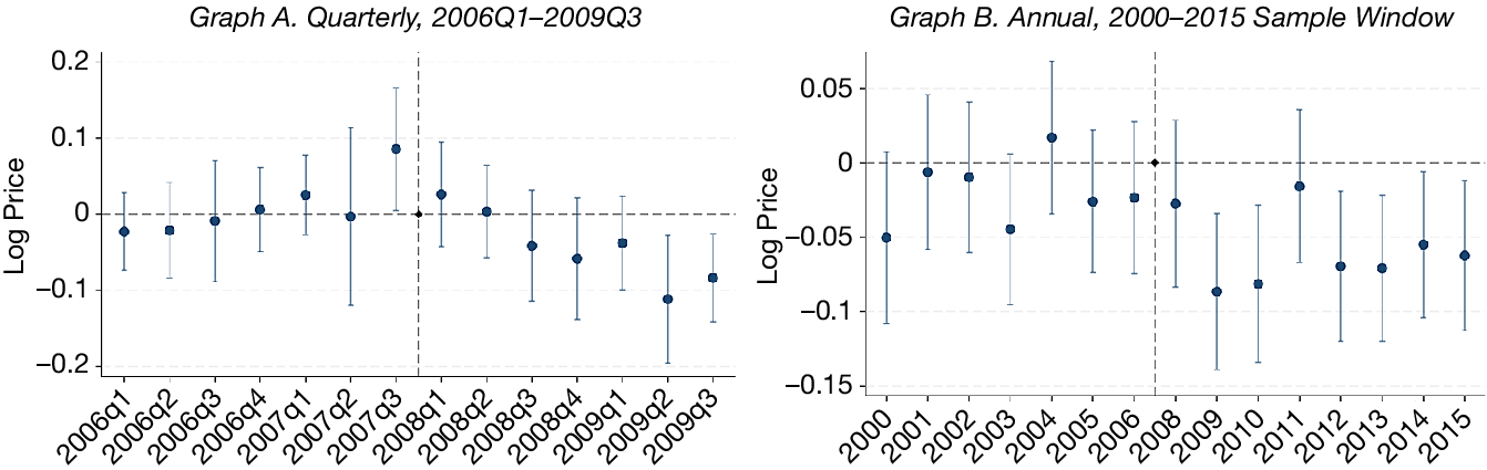
To examine whether the parallel trends assumption holds, I estimate an event-study specification of equation (3) that interacts treatment with calendar-time indicators, taking the map release (2007Q4, or the year 2007 at annual frequency) as the omitted reference period. Graph A of Figure 2 plots the quarterly
$ {Treat}_i\times {Quarter}_t $
 coefficients: the pre-period coefficients are small and jointly insignificant (parallel-trends
$ F $
 -test
$ p=0.46 $
 ), and treated home prices decline steadily after the policy change. Because the quarterly window is short relative to the housing cycle, Graph B extends the event study at annual frequency over the full 2000–2015 sample window, yielding seven pre-period estimates. The treated–control price gap is flat throughout the 2000–2006 California housing boom: the annual pre-period coefficients alternate in sign, none is individually significant at the 5% level, and they are jointly insignificant at the 5% level (
$ F $
 -test
$ p=0.08 $
 ).Footnote
11 Treated homes thus show no differential exposure to the run-up that preceded the policy. Furthermore, the post-period decline is not confined to the 2009–2010 housing market trough: it persists through the 2012–2015 recovery, which is inconsistent with the decline merely reflecting a greater cyclical sensitivity of treated homes. Figure B4 in the Supplementary Material shows that annual transaction counts for treated and control homes track each other closely over the full window. Figure B3 in the Supplementary Material provides additional visual evidence: Graph A shows the all-sales sample with covariates interacted with a linear year trend (
$ F $
 -test
$ p=0.36 $
 ), and Graph B shows the repeat-sales sample with home fixed effects (
$ F $
 -test
$ p=0.12 $
 ).
In Figure 2, event-study estimates of the effect of assignment to a one-level higher wildfire risk zone on logarithm home prices. Each marker is the coefficient on the interaction of the treatment indicator with a calendar-time indicator from a difference-in-differences regression on all sales within 600 m of the new 2007 risk zone boundary, with census-tract, quarter, and year fixed effects and covariates. Graph A: quarterly event time; the omitted reference period is 2007Q4. The pre-period coefficients are jointly insignificant (parallel-trends
$ F $
 -test
$ p=0.46 $
 ). Graph B: annual event time over the 2000–2015 sample window; the omitted reference period is 2007. The pre-period coefficients are individually and jointly insignificant at the 5% level (parallel-trends
$ F $
 -test
$ p=0.08 $
 ). Covariates: age and age squared, home size and home size squared, # bedrooms, # baths, swimming pool dummy, elevation, slope, dummy for location inside the wildland–urban interface, distances to nearest primary road, national forest, state or local park. Vertical bars depict 95% confidence intervals based on heteroscedasticity-robust standard errors. Observations are restricted to census tracts featuring both control and treatment homes.

FIGURE 2 Long description
A two-panel set of event-study plots.
Graph A, titled Quarterly, 2006 Q1 to 2009 Q3, has a y-axis labeled Log Price ranging from negative 0.2 to 0.2 and an x-axis with quarterly time markers. A vertical dashed line marks the treatment event between 2007 Q3 and 2008 Q1. Data points with vertical error bars representing 95 percent confidence intervals show coefficients hovering near zero before the event. After the reference period of 2007 Q4, the coefficients show a downward trend, reaching approximately negative 0.1 by 2009 Q2.
Graph B, titled Annual, 2000 to 2015 Sample Window, has a y-axis labeled Log Price ranging from negative 0.15 to 0.05 and an x-axis with annual markers. A vertical dashed line is placed at the year 2007. Pre-2007 coefficients are mostly negative but statistically insignificant as their error bars cross the zero line. Post-2007, the coefficients remain negative, with the largest drop occurring around 2009 and 2010, followed by a slight recovery but remaining below zero through 2015.
V. Results
A. Effect in the Immediate Vicinity of the New Risk Zone Boundary
1. Regression Discontinuity and Difference-in-Discontinuities Designs
Table 1 contains the RD and RD-DiD estimation results. Using a spatial RD design, the estimated effect of a one-level increase in risk zone on home prices is −6.3% without covariates and −4.0% with covariates (columns 1 and 2, respectively), but not significant at the 10% level. Following Calonico, Cattaneo, and Titiunik (Reference Calonico, Cattaneo and Titiunik2015), the MSE-optimal bandwidth is 209 m and 216 m, without and with covariates, respectively. Running a placebo test for the homes that changed risk zone in 2007 but sold prior to 2007 (denoted hereafter “RD-pre”) also yields insignificant estimates: 0.3% without covariates and 1.0% with covariates (columns 3 and 4, respectively). The MSE-optimal bandwidth in this case is 172 m and 229 m, without and with covariates, respectively.

TABLE 1 Long description
The table consists of six columns of data grouped into three categories: R D (Post) in columns 1 and 2, R D (Pre) in columns 3 and 4, and R D minus D i D in columns 5 and 6.* Row 1: Z = 1. Estimates are minus 0.0631 (0.0410) for column 1, minus 0.0401 (0.0267) for column 2, 0.0034 (0.0405) for column 3, and 0.0099 (0.0285) for column 4. Columns 5 and 6 are empty for this row.* Row 2: Z times Post. Columns 1 through 4 are empty. Estimates are 0.0101 (0.0456) for column 5 and minus 0.0153 (0.0305) for column 6.* Row 3: Number of observations. Values are 3,255 (Col 1), 3,169 (Col 2), 2,850 (Col 3), 3,200 (Col 4), 5,543 (Col 5), and 6,070 (Col 6).* Row 4: Covariates. Columns 2, 4, and 6 are marked ’Yes’, while columns 1, 3, and 5 are blank.* Row 5: Bandwidth (m). Values are 209 (Col 1), 216 (Col 2), 172 (Col 3), 229 (Col 4), 156 (Col 5), and 199 (Col 6).
* Row 1, Z = 1: Column 1 is minus 0.0631 (0.0410); Column 2 is minus 0.0401 (0.0267); Column 3 is 0.0034 (0.0405); Column 4 is 0.0099 (0.0285).
* Row 2, Z times Post: Column 5 is 0.0101 (0.0456); Column 6 is minus 0.0153 (0.0305).
* Row 3, Number of observations: Column 1 is 3255; Column 2 is 3169; Column 3 is 2850; Column 4 is 3200; Column 5 is 5543; Column 6 is 6070.
* Row 4, Covariates: Indicated by checkmarks in columns 2, 4, and 6.
* Row 5, Bandwidth (m): Column 1 is 209; Column 2 is 216; Column 3 is 172; Column 4 is 229; Column 5 is 156; Column 6 is 199.
Standard errors are provided in parentheses below the estimates.
The RD-DiD design accounts for any pre-existing differences across homes on different sides of the new risk zone boundary. Table 1 indicates RD-DiD estimates of 1.0% without covariates and −1.5% with covariates (columns 5 and 6, respectively). The MSE-optimal bandwidth in this case is 156 m and 199 m, without and with covariates, respectively.
The RD and RD-DiD estimates are robust to bandwidths from 100 m to 800 m (Graphs A–C of Figure 3).Footnote 12 Section C of the Supplementary Material reports further checks: the estimates are robust to the polynomial order, to alternative sample selections (including relaxing the census-tract restriction), to alternative boundary cutoffs, and to estimating periods of housing booms and busts separately. The RD estimates are insignificant in every individual year (Table C1 in the Supplementary Material).
In Figure 3, regression discontinuity (RD), difference-in-discontinuities (RD-DiD), and difference-in-differences (DiD) estimates of the effect on logarithm home prices of being located inside a one-level-higher risk zone. Graphs A–C: RD in the post-policy period, RD in the pre-policy period, and RD-DiD estimates, respectively, with bandwidth ranging from 100 to 800 m with 50 m intervals. Regressions include covariates (age, size, number of bedrooms, presence of a swimming pool, distances to the nearest primary road and to the nearest national forest, and dummy for location inside the wildland–urban interface). The vertical blue lines mark half (left) and twice (right) the MSE-optimal bandwidth. Graphs D–F: DiD estimates for regressions that include home, county-by-year, and quarter fixed effects, and robust standard errors. Graph D: bandwidth ranging from 100 to 800 m with 50 m intervals. Graph E: 200 m-ring ranging from 0–200 m to 400–600 m with 50 m intervals. Graph F: 400 m-ring ranging from 0–400 m to 200–800 m with 50 m intervals. In all graphs, the central line depicts the point estimates; the dashed green lines depict the 95% confidence interval. Observations are restricted to census tracts featuring both control and treatment homes.

FIGURE 3 Long description
A multi-panel figure containing six line graphs arranged in two rows of three.
Top Row:
* Graph A. R D, Post-Policy: The x-axis is Bandwidth (m) from 100 to 800. The y-axis is RD Estimate-Post from -0.075 to 0.075. Blue dots show a stable negative estimate around -0.04. Vertical blue dashed lines are at 100 and 400.
* Graph B. R D, Pre-Policy: The x-axis is Bandwidth (m). The y-axis is RD Estimate-Pre. Estimates start near 0.01 at 100m and trend slightly downward toward -0.01 as bandwidth increases.
* Graph C. RD-DiD: The x-axis is Bandwidth (m). The y-axis is RD-DiD Estimate. Estimates start at -0.03, peak near 0 at 300m, then decline steadily to -0.04 at 800m.
Bottom Row:
* Graph D. Di D, Bandwidth: The x-axis is Bandwidth (m). The y-axis is DiD Estimate. Estimates start slightly positive at 100m and trend downward to approximately -0.015 at 800m.
* Graph E. 200m Ring: The x-axis is Outer Edge of Ring (m) from 200 to 600. The y-axis is DiD Estimate from -0.15 to 0.05. Estimates show a U-shaped curve, dipping to -0.07 at 450m before rising slightly.
* Graph F. 400m Ring: The x-axis is Outer Edge of Ring (m) from 400 to 800. The y-axis is DiD Estimate. Estimates show a shallow U-shaped curve, dipping to -0.05 at 600m.
In all panels, a solid blue line connects point estimates, dashed green lines represent 95 percent confidence intervals, and a horizontal black dashed line marks the zero effect level.
2. Difference-in-Differences Design
Columns 1 and 2 in Panel B of Table 2 show the DiD estimates of the effect of being located inside a one-level-riskier zone relative to neighboring control homes that do not change risk zone in the immediate vicinity of the new risk zone boundary. The ATT estimated within 200 m of the new risk zone boundary is −1.1% with census tract, year, and quarter fixed effects plus Covariate
$ \times $
 Year trends (insignificant; column 1) and essentially zero with home and county-by-year fixed effects (insignificant; column 2). These null estimates are consistent with the LATE estimates in Table 1, obtained for a similar bandwidth.

TABLE 2 Long description
The table is divided into two panels.Panel A covers homes 0 to 600 m from the risk zone boundary across four columns.* Row 1, Treat times Post: Column 1 is -0.0411 with significance triple asterisk and standard error 0.0080. Column 2 is -0.0227 with significance triple asterisk and standard error 0.0082. Column 3 is -0.0522 with significance triple asterisk and standard error 0.0089. Column 4 is -0.0152 with significance single asterisk and standard error 0.0085.* Row 2, Number of observations: 8,978 for columns 1 and 2; 6,542 for columns 3 and 4.* Row 3, Adjusted R-squared: 0.85, 0.86, 0.79, and 0.82 respectively.* Fixed Effects (F E) and Controls: All columns include Quarter F E. Columns 1 to 3 include Year F E and Census tract F E. Column 4 includes County times Year F E and Home F E. Covariates are included in columns 1 and 2, with column 2 also including Covariates times Year trend.Panel B covers Finer Distance Bins (Rings) divided into 0 to 200 m (columns 1 and 2) and 200 to 600 m (columns 3 and 4).* Row 1, Treat times Post: Column 1 is -0.0106 (0.0097). Column 2 is 0.0000 (0.0099). Column 3 is -0.0660 with significance triple asterisk (0.0155). Column 4 is -0.0565 with significance triple asterisk (0.0172).* Row 2, Number of observations: 6,074, 4,438, 2,899, and 2,104 respectively.* Row 3, Adjusted R-squared: 0.86, 0.82, 0.85, and 0.84 respectively.* Fixed Effects (F E) and Controls: All columns include Quarter F E. Columns 1 and 3 include Year F E, Census tract F E, Covariates, and Covariates times Year trend. Columns 2 and 4 include County times Year F E and Home F E.
* Row 1, Treat times Post coefficients: Column 1 is -0.0411 (0.0080); Column 2 is -0.0227 (0.0082); Column 3 is -0.0522 (0.0089); Column 4 is -0.0152 (0.0085).
* Row 2, Number of observations: 8978 for columns 1 and 2; 6,542 for columns 3 and 4.
* Row 3, Adjusted R-squared: 0.85, 0.86, 0.79, and 0.82 respectively.
* Fixed Effects (F E) and Controls: All columns include Quarter FE. Columns 1, 2, and 3 include Year FE. Column 4 includes County times Year FE. Columns 1 and 2 include Census tract FE and Covariates. Column 2 adds Covariates times Year trend. Columns 3 and 4 include Home F E.
Panel B covers finer distance rings.
* Columns 1 and 2 (0 to 200 meters), Treat times Post: -0.0106 (0.0097) and 0.0000 (0.0099).
* Columns 3 and 4 (200 to 600 meters), Treat times Post: -0.0660 (0.0155) and -0.0565 (0.0172).
* Number of observations: 6074, 4438, 2899, and 2104 respectively.
* Adjusted R-squared: 0.86, 0.82, 0.85, and 0.84 respectively.
* Fixed Effects (F E) and Controls: All columns include Quarter FE. Columns 1 and 3 include Year F E, Census tract F E, Covariates, and Covariates times Year trend. Columns 2 and 4 include County times Year FE and Home F E.
B. Effect over a Broader Area from the New Risk Zone Boundary
Table 2 shows the main DiD estimates of the effect of being located inside a one-level-riskier zone relative to neighboring control homes that do not change risk zone over a broader area (Panel A) and further away (columns 3 and 4 in Panel B) from the new risk zone boundary.
In Panel A, all homes are located within 600 m of the new 2007 risk zone boundary. Columns 1 through 4 represent specifications with increasingly more flexible fixed effects, with estimates ranging from −5.2% to −1.5%. Column 1 features census tract, year, and quarter fixed effects with home covariates. Column 2 further interacts each covariate with a linear year trend. Columns 3 and 4 feature home fixed effects. The preferred specification (column 4), with home and county-by-year fixed effects to control for regional shocks, yields a price penalty of 1.5%. Graph D of Figure 3 plots this estimate across bandwidths from 100 m to 800 m: it is close to zero at the narrowest bandwidths, which cover the immediate vicinity of the boundary, and settles between 1.2% and 1.5% once the bandwidth exceeds 400 m. In Section C of the Supplementary Material, I also show that estimates are robust to dropping every year in the 2000–2015 time period, one year at a time, or to estimating the model separately during periods of housing booms and busts.
To further understand how the ATT estimates vary spatially, I define spatial rings further away from the new risk zone boundary. The ATT estimates for the 200 m to 600 m ring indicate price penalties of 6.6% and 5.7% (
$ p<0.01 $
 ; columns 3 and 4 in Panel B). Estimates are robust to different choices of ring width and positioning of these rings, from relatively close to relatively far away from the new risk zone boundary (200 m ring in Graph E and 400 m ring in Graph F of Figure 3).Footnote
13
The DiD estimates are robust to a battery of additional checks reported in Section B.2 of the Supplementary Material. First, the Treat
$ \times $
 Post coefficient is negative in every window from
$ \pm $
 2 to
$ \pm $
 8 quarters around the policy date; it becomes significant at the
$ \pm $
 8-quarter window as the sample grows (Table B2 in the Supplementary Material). Second, a 1:1 nearest-neighbor matching-DiD estimator, which matches treated and control homes on pre-period observables, yields ATTs consistent in sign and similar in magnitude to Panel A of Table 2 (Table B3 in the Supplementary Material). Third, replacing the standard control group with type-a controls, homes already carrying the higher hazard rating before 2007, produces a similar spatial gradient as Panel B of Table 2 (Table B5 in the Supplementary Material). Using home, county-by-year, and quarter fixed effects, the 200–600 m ring carries a price penalty of −7.0% (
$ p<0.01 $
 ), while the 0–200 m estimate is economically small and statistically insignificant (−0.8%,
$ p>0.10 $
 ).
VI. Results Interpretation and Potential Mechanisms
This section interprets the joint pattern (null effects at the boundary, significant price penalties further away) and explores mechanisms. If households respond to the risk information contained in the new zone rather than to the salient label, prices should track the underlying wildfire risk. I therefore investigate how wildfire risk varies over space. I leverage high-resolution (30 m
$ \times $
 30 m) wildfire risk measures (not available to households during my sample period), which I map into each home. Then, I run an RD and OLS design with each risk measure as the dependent variable. Table 3 depicts the effect of being located inside a one-level-higher risk zone on the fire risk to homes and the wildfire probability over 30 years. The RD design, Panel A, yields null LATEs on fire risk to homes and wildfire probability over 30 years (
$ p> $
 0.1). In contrast, the OLS approach, Panel B, indicates a 1.8% increase in fire risk to homes over 30 years (
$ p< $
 0.01; columns 1 and 2) and a 2.7% increase in wildfire probability over 30 years for homes located within 600 m of the new 2007 risk zone boundary (
$ p< $
 0.01; columns 3 and 4). These findings suggest that the actual wildfire risk is continuous at the new risk zone boundary and increases further away.

TABLE 3 Long description
The table is organized into four columns of data. Columns 1 and 2 measure Fire Risk to Homes, while columns 3 and 4 measure Wildfire Probability.Panel A. R D Estimates:* Z equals 1: Column 1 is 0.0099 (standard error 0.0087); Column 2 is 0.0134 (standard error 0.0087); Column 3 is 0.0033 (standard error 0.0157); Column 4 is 0.0092 (standard error 0.0159).* Covariates: Included in columns 2 and 4.* N (Sample size): Column 1 is 4397; Column 2 is 4375; Column 3 is 3083; Column 4 is 2981.Panel B. O L S Estimates:* Treat: Column 1 is 0.0184 with three asterisks (standard error 0.0019); Column 2 is 0.0180 with three asterisks (standard error 0.0018); Column 3 is 0.0270 with three asterisks (standard error 0.0027); Column 4 is 0.0269 with three asterisks (standard error 0.0027).* Census tract F E: Yes for all columns.* Covariates: Included in columns 2 and 4.* N (Sample size): Column 1 is 5773; Column 2 is 5640; Column 3 is 5152; Column 4 is 5026.* R sub adj super 2: Column 1 is 0.78; Column 2 is 0.84; Column 3 is 0.81; Column 4 is 0.85.
Panel A presents RD Estimates for the variable Z = 1.
- Row 1 (Coefficients): Column 1 is 0.0099, Column 2 is 0.0134, Column 3 is 0.0033, and Column 4 is 0.0092.
- Row 2 (Standard Errors): Column 1 is 0.0087, Column 2 is 0.0087, Column 3 is 0.0157, and Column 4 is 0.0159.
- Covariates: Included in columns 2 and 4.
- N (Sample Size): Ranges from 2981 to 4397.
Panel B presents OLS Estimates for the variable Treat.
- Row 1 (Coefficients): Column 1 is 0.0184, Column 2 is 0.0180, Column 3 is 0.0270, and Column 4 is 0.0269. All four values are significant at the 1 percent level.
- Row 2 (Standard Errors): Column 1 is 0.0019, Column 2 is 0.0018, Column 3 is 0.0027, and Column 4 is 0.0027.
- Census tract FE: Included in all four columns.
- Covariates: Included in columns 2 and 4.
- N (Sample Size): Ranges from 5026 to 5773.
- R sub adj super 2: Column 1 is 0.78, Column 2 is 0.84, Column 3 is 0.81, and Column 4 is 0.85.
The zone revision could in principle affect prices through both a salience channel and a true-risk channel, and these are not perfectly separable. The null LATE at the boundary, where the discrete zone rating flips but the underlying hazard is essentially continuous (Panel A of Table 3), provides the cleanest evidence on the salience channel. The significant DiD further from the boundary, where average wildfire hazard is genuinely higher inside the zone (Panel B), is informative about the risk-information channel. I acknowledge that this separation is not definitive: the zone boundary reflects CAL FIRE’s hazard model and may encode information that buyers treat as a relevant continuous signal rather than a purely categorical assignment. The joint RD and DiD design provides the best available means to distinguish the two channels given this setting.
In Section E of the Supplementary Material, I explore alternative mechanisms that could influence home prices. Insurance premiums and mortgage market conditions (loan-to-value, mortgage terms, rate spread) show no significant response to the new risk zone. Sales transaction volume in treated areas shows a marginally significant decline of approximately 13%–16% (
$ p<0.10 $
 ) after the rezoning (Table E3 in the Supplementary Material, columns 1–2), with flat pre-trends confirmed by an event study (Figure E1 in the Supplementary Material). This volume decline is consistent with findings in Keys and Mulder (Reference Keys and Mulder2020) that transaction volumes can respond to climate risk, although this effect is weak statistically in my setting.
How does the continuous underlying wildfire risk signal find its way into prices despite the discrete zone assignment? Two nonexclusive market channels plausibly explain this. First, the CAL FIRE maps were publicly available. A buyer considering a home just inside the newly elevated zone could see at a glance that an immediately adjacent home just outside faced nearly identical environmental conditions: the zone boundary is drawn on continuously varying terrain features (fuel load, slope, wind exposure) that do not change discretely at the line. Second, comparable-based valuation may reinforce this mechanism. Appraisers and buyers draw on recent sales from the surrounding neighborhood, which likely spans homes on both sides of a nearby boundary: a home 50 m inside the zone may be routinely compared with homes 50 m outside. If the underlying risk is continuous at the line, this aggregation over the set of comparables would smooth away any pure-risk zone penalty at the boundary. I cannot fully isolate these channels or rule out others, and I state the external-validity claim accordingly.
The comparison with Dessaint and Matray (Reference Dessaint and Matray2017) is instructive about what these results do—and do not—imply. Dessaint and Matray (Reference Dessaint and Matray2017) study salience from the realization of a nearby hurricane: corporate managers increase cash holdings after a vivid, emotionally salient event, a response operating through recency and affect. The salience mechanism here is different in kind: it arises from a policy change (a re-drawn risk map) rather than a realized disaster, and appeals to an assessment of risk probabilities rather than recency or affect. It is therefore consistent that managers over-react to a salient hurricane and that homebuyers may not necessarily over-react to a new map boundary. More broadly, the findings do not imply that salience is unimportant for large assets; rather, they suggest that for infrequently traded assets and nonevent-driven information releases, prices can reflect the continuous underlying risk signal.
The comparison with Donovan et al. (Reference Donovan, Champ and Butry2007) raises a related question of interpretation. In their setting, a home’s risk rating is partially determined by household-level mitigation actions (construction materials, defensible space), making the rating endogenous to households. Homes that find it cheapest to avoid a high rating do so; the remaining high-rated homes are a selected group. The price response on those homes therefore conflates the information effect with selection of nonmitigating households. In my setting, the 2007 zone represents fire hazard at the area level (reflecting fuel load, terrain, and wind patterns) and cannot be changed by household actions. The zone boundary is thus an externally imposed information signal, and the ATT estimates capture the pure information effect without the selection confound.
VII. Conclusions
This article asks whether the salience of climate-related risk affects households’ large asset pricing decisions. I examine how a new wildfire-risk zoning policy in California, whose mandated disclosure makes risk salient at the new zone boundary, affects residential real estate prices. RD, difference-in-discontinuities, and DiD designs in the immediate vicinity of the boundary yield no evidence of an effect on home prices. A DiD design including homes further away yields a −5.7% effect. I interpret these estimates as showing that households do not respond to the increased salience of risk, but update their beliefs in response to the risk information contained in the new zone.
Three implications for asset pricing follow from these findings. First, in this market, newly disclosed risk information is reflected in house prices via the continuous underlying risk signal rather than via the salient discrete classification: the zone level itself does not generate a price penalty at the boundary, but the probability of burning, which is continuous across the boundary and higher on average inside the zone, is priced further inside the zone. Second, the contrast between the null RD result and the significant DiD result would be missed by a design that estimated only an average treatment effect: only the joint use of a discontinuity design and a broader-area design distinguishes a salience effect from an information effect, which has implications for how future studies of climate-risk disclosure are designed. Third, insurance premium quotes did not respond to the rezoning: California regulation prohibited insurers from pricing on zone status in this period. The price decline therefore does not reflect higher insurance costs, consistent with the risk-information channel. Finally, the price decline came with no corresponding adjustment in mortgage loan-to-value ratios (Table E3 in the Supplementary Material), implying that lenders’ effective collateral exposure grew as affected home values fell. This lender nonresponse echoes Keys and Mulder (Reference Keys and Mulder2020), who show that mortgage lenders fail to adjust collateral valuations when federal programs absorb or misprice climate-related risk at below-actuarial rates. These distinctions matter for understanding how climate risk is priced in housing markets and for calibrating the expected effects of disclosure regulation elsewhere.
Supplementary Material
To view supplementary material for this article, please visit http://doi.org/10.1017/S0022109026103494.
Funding Statement
This research received funding from U.S. Forest Service Grant 14-CS-11052007-030 and was part of a project funded by ERC Conservation GA 683031.




 Open access

