


I. Introduction
Exchange rates affect the cost of trade, the returns to international investors, and the transmission of monetary policy across borders, yet their short-horizon movements have resisted consistent prediction. The seminal study of Meese and Rogoff (Reference Meese and Rogoff1983) showed that forecasts based on macroeconomic fundamentals fail to outperform a simple no-change (i.e., random walk without drift) benchmark, and the four decades of research that followed have produced extensive evidence of predictability only at longer horizons (e.g., Mark (Reference Mark1995), Clarida and Taylor (Reference Clarida and Taylor1997), Clarida, Sarno, Taylor, and Valente (Reference Clarida, Sarno, Taylor and Valente2003), Kilian and Taylor (Reference Kilian and Taylor2003), and Eichenbaum, Johannsen, and Rebelo (Reference Eichenbaum, Johannsen and Rebelo2021)). Evidence of out-of-sample predictability at short horizons exists but is more scattered, typically focused on a single fundamental, a single currency, or a limited time span, and robust evidence that fundamental-based forecasts can outperform the no-change benchmark at the monthly frequency over a reasonably long period and for a sizable group of exchange rates remains elusive. This persistent difficulty at short horizons—the finding that fundamentals do not seem to matter for short-horizon exchange rate movements and that the simple no-change forecast has proven so difficult to outperform—is the exchange rate predictability puzzle surveyed by Rossi (Reference Rossi2013).
This article shows that fundamentals do matter for short-horizon exchange rate movements—but their effects vary systematically with global financial conditions. For a panel of 10 developed economies for 1995–2020, we find that monthly U.S. dollar exchange rates are consistently and significantly predictable out of sample once the predictive role of fundamentals is allowed to depend on the global state. Earlier work has shown that allowing for nonlinearity and time variation in predictive relations is important for exchange rate prediction (Kilian and Taylor (Reference Kilian and Taylor2003), Clarida et al. (Reference Clarida, Sarno, Taylor and Valente2003)), but the existing literature has typically been confined to a small number of fundamentals and limited forms of nonlinearity. Our framework combines 10 country-level fundamentals (i.e., characteristics), six global state variables, and their interactions in a high-dimensional panel predictive regression, which we estimate using machine-learning techniques to guard against overfitting in our noisy data environment.
Our predictor set captures a wide range of channels through which fundamentals can move exchange rates. The 10 country characteristics, measured relative to the United States, include inflation rates, unemployment gaps, interest rates at three maturities, equity market valuation ratios, and currency-specific volatility and skewness; each is grounded in a well-known theory of exchange rate determination and is observable to foreign exchange (FX) market participants in real time. The six global state variables comprise indices of economic policy uncertainty, monetary policy uncertainty, and geopolitical risk, together with measures of global FX market volatility, illiquidity, and correlation. We consider numerous country characteristics and global state variables because we cannot know a priori which ones matter most for exchange rate prediction. We then interact every country characteristic with every global state variable, yielding 70 predictors. This lets the predictive effect of each fundamental vary smoothly with the state of the global financial system—something prior work, which typically analyzes nonlinearity within a single fundamental at a time, has not been able to do.
After reserving the first 10 years of data for an initial training sample, we generate monthly out-of-sample forecasts of exchange rate changes by recursively re-estimating the prediction models each month. The out-of-sample period runs from 1995:01 to 2020:09 (2000:02 to 2020:09) for the United Kingdom, Switzerland, Japan, Canada, Australia, New Zealand, Sweden, Norway, and Denmark (Euro area). Due to their adoption of the euro, data for Germany, Italy, France, and the Netherlands end in 1998:12 and are excluded from the out-of-sample analysis (although we use them for training the prediction models).
We estimate the baseline panel predictive regression—which includes the 10 country characteristics and their 60 interactions with the six global state variables—via the elastic net (ENet; Zou and Hastie (Reference Zou and Hastie2005)). The ENet guards against overfitting by shrinking coefficients toward 0 and performs variable selection by shrinking some coefficients to exactly 0. The interaction terms generate continuous regime switching: The predictive effect of each country characteristic varies linearly with each global state variable. To allow for richer nonlinearity, we also fit a deep neural network (DNN) on the same 70 predictors and report an ensemble forecast that averages the ENet and DNN forecasts to harness complementarities between the approaches.Footnote 1
The machine-learning forecasts consistently and significantly outperform the no-change benchmark. Out-of-sample gains are particularly evident when financial distress and market turbulence increase sharply, including during the global financial crisis. Based on the out-of-sample
$ {R}^2 $
 statistic (Fama and French (Reference Fama and French1989), Campbell and Thompson (Reference Campbell and Thompson2008)), which measures the proportional decrease in mean squared prediction error (MSPE) for a competing forecast vis-à-vis a benchmark, the gains are large in the context of the existing literature. The improvements are statistically significant in nearly all cases according to the Clark and West (Reference Clark and West2007) test. For the ensemble forecast, out-of-sample
$ {R}^2 $
 statistics are above 1% (2%) for eight (four) countries, reach 3.41% for the United Kingdom, and produce a composite out-of-sample
$ {R}^2 $
 of 1.86% across the 10 countries (significant at the 1% level). Forecast accuracy also rises significantly with global FX volatility, consistent with a tightening of the link between fundamentals and exchange rates when FX markets become more turbulent.
Beyond predictive performance itself, we investigate the economic drivers underlying the improvements in forecast accuracy. Using the recursive ENet coefficient estimates and the Greenwell, Boehmke, and McCarthy (Reference Greenwell, Boehmke and McCarthy2018) variable-importance measure based on partial dependence plots (PDPs; Friedman (Reference Friedman2001)), we identify a core set of predictors that consistently stand out in the fitted prediction models. Two interactions involving global FX volatility are particularly important. The first is the bill yield differential interacted with global FX volatility: The relation between the bill yield differential and expected U.S. dollar appreciation posited by uncovered interest parity (UIP) strengthens as global FX volatility rises. The second is the inflation differential interacted with global FX volatility: The relation posited by relative purchasing power parity (PPP) likewise strengthens with global FX volatility. Both interactions point to a “flight to fundamentals” in periods of increasing FX market stress, consistent with Clarida, Davis, and Pedersen (Reference Clarida, Davis and Pedersen2009) and Hsu, Taylor, Wang, and Li (Reference Hsu, Taylor, Wang and Li2024), (Reference Hsu, Taylor, Wang and Li2025), who document that carry-trade profitability varies substantially over time and declines markedly when global FX volatility rises. Other predictors that contribute meaningfully include the dividend yield differential and the interaction between the stock market time-series momentum differential and geopolitical risk. Taken together, these findings indicate that the link between fundamentals and exchange rates is conditional, tightening as global financial conditions deteriorate.
Next, we analyze the economic value of the machine-learning forecasts from an investment perspective. We consider a mean–variance U.S. investor with a coefficient of relative risk aversion of 5 who allocates across the U.S. dollar and all available foreign currencies, computing each foreign currency excess return forecast as the bill yield differential minus the expected U.S. dollar appreciation. We label the resulting portfolio the machine-learning optimized (ML-Opt) portfolio when the investor uses a machine-learning forecast of U.S. dollar appreciation and the benchmark-optimized (Bench-Opt) portfolio when the investor uses the no-change benchmark forecast. In the latter case, because the mean–variance investor uses the bill yield differential alone to forecast the currency excess return, the Bench-Opt portfolio can be viewed as an optimal carry-trade portfolio.Footnote 2
Across the different machine-learning forecasts, the ML-Opt portfolios deliver increases in annualized average utility gains of 198 (DNN) to 450 (baseline ENet) basis points over the Bench-Opt portfolio. The gains are present throughout the sample but become especially large starting in late 2008, when the Bench-Opt portfolio’s performance sharply deteriorates—a pattern that tracks the well-documented decline of conventional carry-trade strategies in the wake of the crisis (e.g., Melvin and Taylor (Reference Melvin and Taylor2009), Burnside, Eichenbaum, and Rebelo (Reference Burnside, Eichenbaum and Rebelo2011b), Lustig, Roussanov, and Verdelhan (Reference Lustig, Roussanov and Verdelhan2011), Jordà and Taylor (Reference Jordà and Taylor2012), Daniel et al. (Reference Daniel, Hodrick and Lu2017), Melvin and Shand (Reference Melvin and Shand2017)). Importantly, the ML-Opt portfolios continue to generate sizable, statistically significant alphas in the currency factor model of Lustig et al. (Reference Lustig, Roussanov and Verdelhan2011) both before and after the crisis, even as their carry-factor exposures collapse post-2008—direct evidence that the prediction models pick up time-varying risk exposures.Footnote 3
Our work on resolving the exchange rate predictability puzzle contributes to a time-series forecasting literature that runs parallel to a more recent cross-sectional literature studying exchange rates and fundamentals (e.g., Lustig et al. (Reference Lustig, Roussanov and Verdelhan2011), Colacito, Riddiough, and Sarno (Reference Colacito, Riddiough and Sarno2020), Dahlquist and Hasseltoft (Reference Dahlquist and Hasseltoft2020), Dahlquist and Pénasse (Reference Dahlquist and Pénasse2022), Filippou and Taylor (Reference Filippou and Taylor2023)). These cross-sectional studies construct long-short currency portfolios by sorting on lagged fundamentals—such as interest rate differentials, output gaps, and Taylor (Reference Taylor1993) rule variables—to assess their pricing relevance. In contrast to cross-sectional studies, we generate monthly out-of-sample point forecasts of exchange rate changes, directly analyzing their forecast accuracy as well as their economic value via our ML-Opt and Bench-Opt portfolios. In sum, we go beyond the ordinal information in currency sorts by using point forecasts of exchange rate changes, which incorporate information about both the sign and magnitude of expected movements in a time-series forecasting context to address the exchange rate predictability puzzle. The relatively small number of available currencies also limits the number of fundamentals that can be analyzed in a sort-based framework. Our predictive regression approach instead accommodates a large number of characteristics and their interactions with global state variables.
The remainder of the article is organized as follows: Section II describes the data. Section III discusses the model specification and construction of the machine-learning forecasts. Section IV presents results on out-of-sample forecast accuracy. Section V analyzes the economic drivers of the forecasts. Section VI constructs the mean–variance optimal portfolios and measures the economic value of the machine-learning forecasts. Section VII concludes.
II. Data
This section describes the data used in our analysis.
A. Exchange Rates
We begin with daily exchange rate data from Barclays and Reuters via Datastream. We convert daily spot exchange rates to a monthly frequency using end-of-month values (e.g., Burnside, Eichenbaum, Kleshchelski, and Rebelo (Reference Burnside, Eichenbaum, Kleshchelski and Rebelo2011a), Lustig et al. (Reference Lustig, Roussanov and Verdelhan2011)). Our sample consists of currencies for the Euro area and 13 countries: the United Kingdom, Switzerland, Japan, Canada, Australia, New Zealand, Sweden, Norway, Denmark, Germany, Italy, France, and the Netherlands. Our universe of exchange rates is similar to the sample of developed countries employed in other studies (e.g., Lustig et al. (Reference Lustig, Roussanov and Verdelhan2011), Menkhoff, Sarno, Schmeling, and Schrimpf (Reference Menkhoff, Sarno, Schmeling and Schrimpf2012a)). The Euro area replaces Germany, Italy, France, and the Netherlands after the Euro’s introduction in 1999. We use
$ {S}_{i,t} $
 to denote the month-
$ t $
 spot exchange rate for country
$ i $
 , expressed as the number of country-
$ i $
 currency units per U.S. dollar (e.g., Lustig et al. (Reference Lustig, Roussanov and Verdelhan2011), Menkhoff et al. (Reference Menkhoff, Sarno, Schmeling and Schrimpf2012a), Menkhoff, Sarno, Schmeling, and Schrimpf (Reference Menkhoff, Sarno, Schmeling and Schrimpf2012b)). An increase in
$ {S}_{i,t} $
 thus represents an appreciation of the U.S. dollar. The country-
$ i $
 log exchange rate change is denoted by
$ \Delta {s}_{i,t}={s}_{i,t}-{s}_{i,t-1} $
 , where
$ {s}_{i,t}=\ln \left({S}_{i,t}\right) $
 . Except for four countries, the sample ends in 2020:09; for France, Germany, Italy, and the Netherlands, the sample ends in 1998:12, the last month for which these countries had their own currencies. Based on data availability for the predictors, the sample begins in 1985:01 for all countries, except for the Euro area, where the sample begins in 1999:02, corresponding to the introduction of the Euro in January of 1999.Footnote
4
B. Country Characteristics
We consider a large set of country characteristics based on a variety of macroeconomic and financial variables, all of which are based on data available to FX market participants. Section A.1 of the Appendix provides more detailed descriptions of the predictors and the motivation for their inclusion. Specifically, we consider 10 monthly country characteristics: i) inflation differential (
$ {\mathrm{INF}}_{i,t} $
 ), ii) unemployment rate gap differential (
$ {\mathrm{UN}}_{i,t} $
 ), iii) bill yield differential (
$ {\mathrm{BILL}}_{i,t} $
 ), iv) note yield differential (
$ {\mathrm{NOTE}}_{i,t} $
 ), v) bond yield differential (
$ {\mathrm{BOND}}_{i,t} $
 ), vi) dividend yield differential (
$ {\mathrm{DP}}_{i,t} $
 ), vii) price–earnings ratio differential (
$ {\mathrm{PE}}_{i,t} $
 ), viii) stock market time-series momentum differential (
$ \mathrm{SRET}{12}_{i,t} $
 ), ix) idiosyncratic volatility (
$ {\mathrm{IV}}_{i,t} $
 ), and x) idiosyncratic skewness (
$ {\mathrm{IS}}_{i,t} $
 ). All the differentials are measured as the country-
$ i $
 value minus the U.S. value. IV and IS are computed using fitted residuals for the Lustig et al. (Reference Lustig, Roussanov and Verdelhan2011) 2-factor model estimated using daily data for month
$ t $
 for country-
$ i $
 log currency excess returns. The characteristics are based on popular predictors from the literature that relate to well-known theories, such as relative PPP, Taylor-rule fundamentals, UIP, and uncovered equity parity (UEP).
C. Global State Variables
Given that we are generating short-horizon forecasts, allowing for state variables that may influence short-term market sentiment is important. We term these global variables, although the first two relate mainly to the United States, because they all likely affect U.S. dollar exchange rates. We consider six monthly global variables: i) economic policy uncertainty (
$ {\mathrm{EPU}}_t $
 ; Baker, Bloom, and Davis (Reference Baker, Bloom and Davis2016)), ii) monetary policy uncertainty (
$ {\mathrm{MPU}}_t $
 ; Baker et al. (Reference Baker, Bloom and Davis2016)), iii) geopolitical risk (
$ {\mathrm{GR}}_t $
 ; Caldara and Iacoviello (Reference Caldara and Iacoviello2022)), iv) global FX volatility (
$ {\mathrm{GVOL}}_t $
 ; Menkhoff et al. (Reference Menkhoff, Sarno, Schmeling and Schrimpf2012a)), v) global FX illiquidity (
$ {\mathrm{GILL}}_t $
 ; Menkhoff et al. (Reference Menkhoff, Sarno, Schmeling and Schrimpf2012a)), and vi) global FX correlation (
$ {\mathrm{GCOR}}_t $
 ; Mueller, Stathopoulos, and Vedolin (Reference Mueller, Stathopoulos and Vedolin2017)).Footnote
5 Each captures general conditions that can affect the predictive ability of the country characteristics.
III. Panel Predictive Regressions
In this section, we specify the baseline panel predictive regression and DNN models used to construct the out-of-sample forecasts and the ensemble forecast.
A. Baseline Specification
We denote the collection of characteristics in Section II for country
$ i $
 and month
$ t $
 by
$ {\left\{{z}_{j,i,t}\right\}}_{j=1}^J $
 , where
$ J=10 $
 , for
$ i=1,\dots, N $
 , and
$ t=1,\dots, T $
 .Footnote
6 The collection of global state variables in Section II is denoted by
$ {\left\{{g}_{k,t}\right\}}_{k=1}^K $
 , where
$ K=6 $
 . We interact each country characteristic with the set of global variables, yielding the set
$ {\left\{{\left\{{z}_{j,i,t}\hskip0.1em {g}_{k,t}\right\}}_{k=1}^K\right\}}_{j=1}^J $
 . After standardizing all the predictors, our baseline panel predictive regression is given by

for
$ i=1,\dots, N $
 and
$ t=1,\dots, T-1 $
 , where
$ {\tilde{z}}_{j,i,t} $
 (
$ \tilde{z_{j,i,t}\hskip0.1em {g}_{k,t}} $
 ) is the standardized country characteristic (interaction term),
$ {\mu}_{j,i}^z $
 (
$ {\mu}_{j,i,k}^{z,g} $
 ) is the mean of
$ {z}_{j,i,t} $
 (
$ {z}_{j,i,t}\hskip0.1em {g}_{k,t} $
 ),
$ {\sigma}_{j,i}^z $
 (
$ {\sigma}_{j,i,k}^{z,g} $
 ) is the standard deviation of
$ {z}_{j,i,t} $
 (
$ {z}_{j,i,t}\hskip0.1em {g}_{k,t} $
 ), and
$ {\varepsilon}_{i,t+1} $
 is a zero-mean disturbance term.
Equation (1) is high dimensional, as it includes
$ J\left(K+1\right)=10\times 7=70 $
 predictors. We include many more predictors than existing studies of exchange rate predictability, which typically consider only a limited number of country characteristics. The inclusion of a broad set of characteristics is germane, because we do not know a priori which are relevant for forecasting exchange rates. It also helps guard against data mining or snooping, as we include an extensive set of potentially relevant fundamentals in the model from the start. In addition to numerous country characteristics, we include their interactions with the set of global variables, which allows for the predictive relations between exchange rate changes and fundamentals to vary with global economic conditions. To the best of our knowledge, such interactions have not previously been considered in the out-of-sample exchange rate predictability literature.
Equation (1) also pools the data, thereby restricting the response of
$ \Delta {s}_{i,t+1} $
 to
$ {\tilde{z}}_{j,i,t} $
 and
$ \tilde{z_{j,i,t}\hskip0.1em {g}_{k,t}} $
 to be the same across
$ i $
 . These slope homogeneity restrictions reduce the parameter space to help guard against overfitting. Although the slope homogeneity restrictions are unlikely to hold exactly—potentially inducing bias in the parameter estimates—they also decrease the variance of the parameter estimates, which can improve out-of-sample performance in light of the bias–variance trade-off. Whether pooling is beneficial is ultimately an empirical issue determined by the bias–variance trade-off; for our application, we find that pooling leads to better time-series forecasts of individual exchange rates.Footnote
7
Furthermore, observe that equation (1) does not include an intercept term. Because the predictors are in deviation form, we effectively impose the restrictions that the country-specific means for
$ \Delta {s}_{i,t} $
 for
$ i=1,\dots, N $
 are 0. In other words, equation (1) is tantamount to a fixed-effects specification in which the country-specific means for the log exchange rate changes are all 0. These 0 restrictions are consistent with economic intuition and the data, and they further reduce the number of parameters that we need to estimate, again helping to guard against overfitting in light of the bias–variance trade-off.
1. Regime Switching
The inclusion of the interaction terms in equation (1) effectively permits a form of regime switching in the predictive relations between the country characteristics and exchange rate changes. To see this, note that the response of
$ \Delta {s}_{i,t+1} $
 to a change in
$ {z}_{j,i,t} $
 in equation (1) is given by

for
$ j=1,\dots, J $
 and
$ i=1,\dots, N $
 . According to equation (2), the slope coefficient for
$ {z}_{j,i,t} $
 varies linearly with
$ {g}_{k,t} $
 for
$ k=1,\dots, K $
 . For example, if
$ {\beta}_{j,k}^{z,g}>0 $
 , then the response of
$ \Delta {s}_{i,t+1} $
 to a change in
$ {z}_{j,i,t} $
 increases linearly with
$ {g}_{k,t} $
 . We refer to equation (1) and the concomitant response in equation (2) as encapsulating continuous regime switching. Setting
$ {\beta}_{j,k}^{z,g}=0 $
 for
$ j=1,\dots, J $
 and
$ k=1,\dots, K $
 in equation (1) (i.e., excluding the interaction terms) produces a panel predictive regression based on the country characteristics alone:

where the number of predictors is reduced to
$ J=10 $
 . For equation (3), the derivative in equation (2) simplifies to the first term on the right-hand side (
$ {\beta}_j^z\hskip0.1em (1/{\sigma}_{j,i}^z) $
 ), so regime switching is absent.
2. Elastic Net
An out-of-sample forecast of
$ \Delta {s}_{i,T+1} $
 based on the baseline panel predictive regression in equation (1) and data available through
$ T $
 is given by

where
$ {\hat{\beta}}_j^z $
 and
$ {\hat{\beta}}_{j,k}^{z,g} $
 are estimates of
$ {\beta}_j^z $
 and
$ {\beta}_{j,k}^{z,g} $
 , respectively, in equation (1) for
$ j=1,\dots, J $
 and
$ k=1,\dots, K $
 based on data available through
$ T $
 . The plugged-in predictors on the right-hand side of equation (4),
$ {\tilde{z}}_{j,i,T} $
 and
$ \tilde{z_{j,i,T}\hskip0.1em {g}_{k,T}} $
 , are standardized using data through
$ T $
 . By estimating the slope coefficients and standardizing the predictors using data available through
$ T $
 (i.e., the time of forecast formation), we avoid “look-ahead” bias in the forecast.
Even after imposing the slope homogeneity and zero-mean restrictions in equation (1), because the panel predictive regression is high dimensional and the unpredictable component in monthly exchange rate changes is inherently large, conventional OLS estimation of the parameters
$ {\beta}_j^z $
 and
$ {\beta}_{j,k}^{z,g} $
 for
$ j=1,\dots, J $
 and
$ k=1,\dots, K $
 is highly susceptible to overfitting. Thus, we consider penalized (or regularized) regression, which shrinks the parameter estimates toward 0 to reduce their variance and improve out-of-sample performance according to the bias–variance trade-off.
We employ penalized regression via the ENet (Zou and Hastie (Reference Zou and Hastie2005)), a popular and powerful machine-learning technique that mitigates overfitting by including a penalty term in the objective function for estimating equation (1). Collecting the parameters in the vector
$ \underset{J\left(K+1\right)}{\boldsymbol{\beta}}={\left[{\beta}_1^z\hskip0.5em \cdots \hskip0.5em {\beta}_J^z\hskip0.5em {\beta}_{1,1}^{z,g}\hskip0.5em \cdots \hskip0.5em {\beta}_{1,K}^{z,g}\hskip0.5em \cdots \hskip0.5em {\beta}_{J,1}^{z,g}\hskip0.5em \cdots \hskip0.5em {\beta}_{J,K}^{z,g}\right]}^{\prime } $
 , the ENet objective function can be expressed as

where
$ \lambda \ge 0 $
 is a regularization hyperparameter that governs the degree of shrinkage;
$ \parallel \cdot {\parallel}_1 $
 and
$ \parallel \cdot {\parallel}_2 $
 are the
$ {\mathrm{\ell}}_1 $
 and
$ {\mathrm{\ell}}_2 $
 norms, respectively; and
$ \delta $
 is a blending hyperparameter for the
$ {\mathrm{\ell}}_1 $
 and
$ {\mathrm{\ell}}_2 $
 components in the penalty term.Footnote
8 When
$ \lambda =0 $
 , there is no shrinkage, so the ENet and OLS objective functions coincide; when
$ \lambda >0 $
 , the penalty term shrinks the parameter estimates toward 0 to mitigate overfitting. The ENet penalty term in equation (5) includes both
$ {\mathrm{\ell}}_1 $
 (least absolute shrinkage and selection operator or LASSO; Tibshirani (Reference Tibshirani1996)) and
$ {\mathrm{\ell}}_2 $
 (ridge; Hoerl and Kennard (Reference Hoerl and Kennard1970)) components. The former permits shrinkage to 0 (for sufficiently large
$ \lambda $
 ), so the ENet performs variable selection (i.e., can produce a sparse model).Footnote
9 We tune the hyperparameters
$ \lambda $
 and
$ \delta $
 via the extended regularized information criterion (ERIC; Hui, Warton, and Foster (Reference Hui, Warton and Foster2015)), which is a relatively stringent information criterion, because it tends to induce more shrinkage than cross-validation and other information criteria.Footnote
10 Considering grids of values for
$ \lambda $
 and
$ \delta $
 , we select the values that minimize the ERIC. Given our high-dimensional and noisy data environment, the ERIC appears effective for tuning the hyperparameters.
B. Deep Neural Network
The baseline specification in equation (1) permits nonlinearities in the predictors through the interaction terms. To allow for additional nonlinearities, we consider the following general panel predictive regression:

for
$ i=1,\dots, N $
 and
$ t=1,\dots, T-1 $
 , where
$ \underset{J\left(K+1\right)}{{\tilde{\boldsymbol{x}}}_{i,t}}=\Big[{\displaystyle \begin{array}{ccccc}{\tilde{z}}_{1,i,t}& \cdots & {\tilde{z}}_{J,i,t}& \tilde{z_{1,i,t}\hskip0.1em {g}_{1,t}}& \cdots \end{array}} $
 $ {\displaystyle \begin{array}{ccccc}\tilde{z_{1,i,t}\hskip0.1em {g}_{K,t}}& \cdots & \tilde{z_{J,i,t}\hskip0.1em {g}_{1,t}}& \cdots & \tilde{z_{J,i,t}\hskip0.1em {g}_{K,t}}\end{array}}\Big]{}^{\prime } $
 and
$ f\left({\tilde{\boldsymbol{x}}}_{i,t}\right) $
 is a generic function constituting the conditional expectation function. We model
$ f\left({\tilde{\boldsymbol{x}}}_{i,t}\right) $
 in equation (6) via a DNN, a popular machine-learning device for flexibly modeling complex relations between predictors and a target variable. A feedforward neural network is composed of multiple layers. The first is the input layer, which is simply the set of predictors. One or more hidden layers are next, where each hidden layer contains multiple neurons with a nonlinear activation function. The input layer is densely connected to the first hidden layer, and each subsequent hidden layer is densely connected to its preceding hidden layer. The neurons produce signals that are passed forward through the hidden layers. Finally, an output layer translates the signals from the last hidden layer into a prediction.
It is well known that a neural network with a single hidden layer and a sufficiently large number of neurons can, theoretically, approximate any smooth function (e.g., Hornik, Stinchcombe, and White (Reference Hornik, Stinchcombe and White1989)). However, neural networks with multiple hidden layers (i.e., DNNs) and a more limited number of neurons in each layer often perform better in practice than neural networks with one hidden layer and a large number of neurons (e.g., Goodfellow, Bengio, and Courville (Reference Goodfellow, Bengio and Courville2016), Gu et al. (Reference Gu, Kelly and Xiu2020)). Our DNN has four hidden layers with 16, 8, 4, and 2 neurons, respectively, with dense connections between adjacent layers and a single output node producing the exchange rate change forecast. The specification of 16 neurons in the first hidden layer is a compromise between two popular rules of thumb: half or the square root of the number of predictors. Section IA.2 of the Supplementary Material provides further details on the architecture, activation function, and estimation strategy, including the steps that we take to guard against overfitting in our noisy data environment. As in the baseline panel predictive regression in equation (1), the DNN predicts a value of 0 for the exchange rate change when all of the (standardized) predictors are at their mean value of 0.
C. Ensemble
We also compute an ensemble forecast by taking the average of the ENet and DNN forecasts, which provides a convenient strategy for blending the different forecast strategies. An average of multiple individual forecasts is known as a “voting ensemble” in the machine-learning literature. An ensemble forecast recognizes that we do not know the best individual model a priori and allows us to take advantage of potential complementarities between models.
IV. Out-of-Sample Performance
In this section, we analyze the accuracy of the out-of-sample machine-learning forecasts and their ability to resolve the short-horizon exchange rate predictability puzzle.
A. Forecast Construction
Mimicking the situation of a forecaster in real time, we generate exchange rate forecasts for the 1995:01–2020:09 out-of-sample period as follows: Reserving the first 10 years of data (1985:01–1994:12) for the initial training sample, we estimate the baseline panel predictive regression in equation (1) and the DNN in Section III.B using data available through 1994:12. We then use the fitted prediction models and 1994:12 predictor values for each country to compute forecasts for 1995:01. Next, we re-estimate the models using data available through 1995:01 and use the fitted models and 1995:01 predictor values for each country to generate forecasts for 1995:02. We continue in this fashion through the end of the out-of-sample period, providing us with a set of exchange rate forecasts for the available countries for each of the 309 months comprising the out-of-sample period. By retraining the prediction models each month as new data become available, we update the fitted models in a timely manner; similarly, we also regularly retune the hyperparameters.Footnote 11 Note that there is no look-ahead bias in the forecasts, as we only use data available at the time of forecast formation when training the models (and standardizing the predictors).
For Germany, Italy, France, and the Netherlands, there are only 48 monthly forecasts (1995:01–1998:12) available for evaluation, due to these countries joining the Euro area in 1999:01. Thus, we do not include these four countries when evaluating forecast performance. However, we use data for these countries when training the prediction models, as this increases the number of training-sample observations, thereby improving estimation efficiency. After imposing a minimum requirement of 12 monthly observations before a currency is included in the panel predictive regression, there are 248 forecasts (2000:02–2020:09) available for the Euro area. For the remaining nine countries, forecasts are available for the entire 1995:01–2020:09 out-of-sample period (309 observations). In addition to reporting results for the individual countries, we report results for the entire collection of countries taken together (excluding Germany, Italy, France, and the Netherlands, resulting in
$ 248+9\times 309=\mathrm{3,029} $
 observations).
B. Test Statistics
We compare competing forecasts that incorporate information from economic fundamentals to the no-change benchmark, the most stringent benchmark for out-of-sample exchange rate prediction (Rossi (Reference Rossi2013)). For country
$ i $
 , we can conveniently compare the relative accuracy of a competing forecast vis-à-vis the no-change benchmark in terms of MSPE in the time-series dimension using the out-of-sample
$ {R}^2 $
 statistic (Fama and French (Reference Fama and French1989), Campbell and Thompson (Reference Campbell and Thompson2008)):

where
$ {\hat{e}}_{i,t\mid t-1}^j=\Delta {s}_{i,t}-{\hat{\Delta s}}_{i,t\mid t-1}^j $
 for
$ j=\mathrm{Bench},\mathrm{Compete} $
 ;
$ {\hat{\Delta s}}_{i,t\mid t-1}^{\mathrm{Bench}}=0 $
 is the no-change benchmark forecast;
$ {\hat{\Delta s}}_{i,t\mid t-1}^{\mathrm{Compete}} $
 is a competing forecast;
$ {T}_1 $
 is the last observation for the initial in-sample period; and
$ {T}_2 $
 is the last available observation for the out-of-sample period. The
$ {R}_{i,\mathrm{OS}}^2 $
 statistic measures the proportional reduction in MSPE for a competing forecast vis-à-vis the benchmark. Because the predictable component in monthly exchange rate changes is intrinsically small, the
$ {R}_{i,\mathrm{OS}}^2 $
 statistic will necessarily be small. Nevertheless, even a seemingly small degree of monthly exchange rate predictability can be economically meaningful, as we show in Section VI and as is the case for stock return predictability (Campbell and Thompson (Reference Campbell and Thompson2008)).
To test whether the competing forecast provides a statistically significant improvement in MSPE relative to the benchmark when comparing nested models, we compute the Clark and West (Reference Clark and West2007) adjusted version of the popular Diebold and Mariano (Reference Diebold and Mariano1995) and West (Reference West1996) statistic. Specifically, we use the Clark and West (Reference Clark and West2007) statistic to test (in population)
$ {H}_0 $
 :
$ {\mathrm{MSPE}}^{\mathrm{Bench}}\le {\mathrm{MSPE}}^{\mathrm{Compete}} $
 (
$ {R}_{i,\mathrm{OS}}^2\le 0 $
 ) against
$ {H}_A $
 :
$ {\mathrm{MSPE}}^{\mathrm{Bench}}>{\mathrm{MSPE}}^{\mathrm{Compete}} $
 (
$ {R}_{i,\mathrm{OS}}^2>0 $
 ). For country
$ i $
 , the Clark and West (Reference Clark and West2007) statistic can be conveniently computed using the
$ t $
 -statistic corresponding to the intercept term (
$ {a}_{0,i} $
 ) in the following regression:

for
$ t={T}_1+1,\dots, {T}_2 $
 , where
$ {l}_{i,t} $
 is the adjusted loss differential. Clark and West (Reference Clark and West2007) show that the
$ t $
 -statistic corresponding to
$ {a}_{0,i} $
 in equation (8) is well approximated by the standard normal distribution under the null hypothesis.
We also compute a composite out-of-sample
$ {R}^2 $
 statistic based on the entire collection of countries taken together:

For testing
$ {H}_0 $
 :
$ {R}_{\mathrm{All},\mathrm{OS}}^2\le 0 $
 against
$ {H}_A $
 :
$ {R}_{\mathrm{All},\mathrm{OS}}^2>0 $
 , we compute a pooled version of the Clark and West (Reference Clark and West2007) statistic by calculating the
$ t $
 -statistic corresponding to the intercept term (
$ {a}_0 $
 ) in the following regression:

for
$ i=1,\dots, N $
 and
$ t={T}_1+1,\dots, {T}_2 $
 , where we cluster the standard errors by country and time. A caveat to the
$ {R}_{\mathrm{All},\mathrm{OS}}^2 $
 statistic is that it can reflect cross-sectional as well as time-series predictability, whereas, in line with the exchange rate predictability puzzle, we are interested in the latter. With this caveat in mind, we report the
$ {R}_{\mathrm{All},\mathrm{OS}}^2 $
 statistic in equation (9) to provide an overall measure of the accuracy of the exchange rate forecasts for the entire group of countries taken together.
C. Forecast Accuracy: Outperforming the Random Walk
Table 1 reports the
$ {R}_{i,\mathrm{OS}}^2 $
 statistic in equation (7) for different forecasts and the 10 countries for which we have at least 248 monthly observations for the forecast evaluation period. It also reports the
$ {R}_{\mathrm{All},\mathrm{OS}}^2 $
 statistic in equation (9) for the 10 countries taken together. The fourth and fifth columns of the table report results for forecasts based on the baseline panel predictive regression in equation (1) estimated via OLS (baseline OLS) and the ENet (baseline ENet), respectively, whereas the sixth column provides results for the panel predictive regression without interaction terms in equation (3) estimated via the ENet (no-interaction ENet). Finally, the seventh and eighth columns report results for the DNN in Section III.B and the ensemble forecast in Section III.C (an average of the baseline ENet and DNN forecasts), respectively.Footnote
12

TABLE 1 Long description
The table consists of 8 columns: Country, Out-of-Sample Period, Number of Observations, Baseline O L S, Baseline ENet, No-Interaction ENet, D N N, and Ensemble.
* The Out-of-Sample Period for most countries is 1995:01 to 2020:09 with 309 observations, except for the Euro area (2000:02 to 2020:09, 248 observations) and the ‘All’ aggregate (3,029 observations).
* Baseline O L S shows negative values for all entries, ranging from -3.21 (Norway) to -19.75 (Canada).
* Baseline ENet shows positive, significant results for the United Kingdom (3.24), Australia (1.47), New Zealand (2.15), Sweden (1.86), Norway (1.91), Denmark (2.23), and Euro area (2.38).
* No-Interaction ENet has lower performance, with several negative values and only small positive significant results for the United Kingdom, Australia, New Zealand, Norway, and Denmark.
* D N N (Deep Neural Network) shows consistently positive and significant results for most countries, notably 3.03 for the United Kingdom and 2.15 for Switzerland.
* Ensemble (average of ENet and D N N) provides the highest or near-highest R super 2 values for most rows, including 3.41 for the United Kingdom and 2.65 for the Euro area.
* The ‘All’ aggregate row shows significant R super 2 values for Baseline ENet (1.51), D N N (1.74), and Ensemble (1.86), while Baseline O L S (-8.74) and No-Interaction ENet (-0.29) are negative.
The
$ {R}_{i,\mathrm{OS}}^2 $
 and
$ {R}_{\mathrm{All},\mathrm{OS}}^2 $
 statistics are all negative in the fourth column of Table 1, so the baseline OLS forecast always fails to outperform the no-change benchmark. The negative
$ {R}_{i,\mathrm{OS}}^2 $
 statistics are often quite sizable in magnitude for the individual countries, and the
$ {R}_{\mathrm{All},\mathrm{OS}}^2 $
 statistic is
$ -8.74\% $
 for the 10 countries taken together in the last row. Its poor out-of-sample performance indicates that the baseline OLS forecast substantially overfits the data, which is not surprising in our high-dimensional and noisy data environment.
As reported in the fifth column of Table 1, employing shrinkage to mitigate overfitting proves highly beneficial, as the baseline ENet forecast evinces markedly better out-of-sample performance than the baseline OLS forecast. Specifically, the
$ {R}_{i,\mathrm{OS}}^2 $
 statistics are positive for 8 of the 10 countries for the baseline ENet forecast, and the reduction in MSPE relative to the no-change benchmark is significant at conventional levels for seven of the eight countries. Seven (four) of the
$ {R}_{i,\mathrm{OS}}^2 $
 statistics are above 1% (2%) and reach as high as 3.24% (the United Kingdom), so they are sizable in the context of the literature on out-of-sample exchange rate predictability. For the complete set of countries taken together, the
$ {R}_{\mathrm{All},\mathrm{OS}}^2 $
 statistic is 1.51% (significant at the 5% level).
The sixth column of Table 1 reports results for the no-interaction ENet forecast. This forecast is based on the panel predictive regression without interaction terms in equation (3), which, as discussed in Section III.A, is akin to restricting the slope coefficients for the country characteristics to be constant (i.e., no regime switching). The
$ {R}_{i,\mathrm{OS}}^2 $
 statistics are positive for 5 of the 10 countries, and all 5 are significant at conventional levels. Taking the 10 countries together, the
$ {R}_{\mathrm{All},\mathrm{OS}}^2 $
 statistic is negative (
$ -0.29\% $
 ). Overall, there is some evidence that using country characteristics without regime switching outperforms the no-change benchmark. However, comparing the results in the fifth and sixth columns of Table 1, the
$ {R}_{i,\mathrm{OS}}^2 $
 and
$ {R}_{\mathrm{All},\mathrm{OS}}^2 $
 statistics are all larger for the baseline ENet forecast vis-à-vis the no-interaction ENet forecast, often by a substantial margin. Thus, we have strong evidence that allowing for regime switching in the responses of exchange rate changes to characteristics improves out-of-sample predictability.
According to the seventh column of Table 1, the DNN forecast performs well. The
$ {R}_{i,\mathrm{OS}}^2 $
 statistics are positive for all countries, with significant improvements in MSPE relative to the no-change benchmark for eight of them. Like those for the baseline ENet forecast, the
$ {R}_{i,\mathrm{OS}}^2 $
 statistics for the individual countries are sizable, and eight (four) are above 1% (2%), with a maximum of 3.03% (the United Kingdom). For the 10 countries considered jointly, the
$ {R}_{\mathrm{All},\mathrm{OS}}^2 $
 statistic is 1.74% for the DNN forecast (significant at the 1% level).
By combining the baseline ENet and DNN forecasts, the ensemble approach in the last column of Table 1 provides the best overall performance. The
$ {R}_{i,\mathrm{OS}}^2 $
 statistics are positive for all 10 countries, and the improvements in MSPE vis-à-vis the no-change benchmark are significant for eight of them. The
$ {R}_{i,\mathrm{OS}}^2 $
 statistics are also often quite sizable, with eight (four) above 1% (2%), and the maximum is 3.41% (the United Kingdom). For the 10 countries taken together, the
$ {R}_{\mathrm{All},\mathrm{OS}}^2 $
 statistic is 1.86% (significant at the 1% level). Note that for a number of countries, the
$ {R}_{i,\mathrm{OS}}^2 $
 statistic for the ensemble forecast is larger than the highest corresponding statistic in the fifth and seventh columns, pointing to meaningful complementarities in the baseline ENet and DNN forecasts.Footnote
13
To examine the performance of the baseline ENet, DNN, and ensemble forecasts over time, Figure 1 shows rolling 60-month
$ {R}_{i,\mathrm{OS}}^2 $
 and
$ {R}_{\mathrm{All},\mathrm{OS}}^2 $
 statistics for the baseline ENet, DNN, and ensemble forecasts (considered in turn). The horizontal axes in Figure 1 correspond to the end of the 60-month rolling window. Figure 1 demonstrates that our machine-learning approach consistently generates out-of-sample gains over time. Except for Japan, the clear majority of the rolling 60-month
$ {R}_{i,\mathrm{OS}}^2 $
 statistics are positive for the individual countries, and the
$ {R}_{\mathrm{All},\mathrm{OS}}^2 $
 statistics for the ensemble forecast are positive for nearly every 60-month window. The rolling
$ {R}_{i,\mathrm{OS}}^2 $
 and
$ {R}_{\mathrm{All},\mathrm{OS}}^2 $
 statistics are quite large for 60-month windows that include the nadir of the global financial crisis in late 2008, with values above 6% in many cases. Substantive out-of-sample gains are also evident outside of the crisis. For example, for numerous countries, including Switzerland, Australia, Sweden, Norway, and Denmark, the
$ {R}_{i,\mathrm{OS}}^2 $
 statistics are relatively large for windows ending in the early 2000s. In addition,
$ {R}_{i,\mathrm{OS}}^2 $
 statistics are sizable for windows ending in the later part of the out-of-sample period for Switzerland, Japan, Sweden, Norway, and Denmark. Along this line, the
$ {R}_{i,\mathrm{OS}}^2 $
 statistics for 60-month windows ending around 2004–2006 are substantive for countries such as the United Kingdom, Canada, Australia, and New Zealand.Footnote
14 Overall, Table 1 and Figure 1 indicate that the information in our large set of predictors and machine-learning methods can be used to generate sizable and consistent improvements in out-of-sample forecast accuracy.
Figure 1 depicts rolling 60-month
$ {R}_{i,\mathrm{OS}}^2 $
 and
$ {R}_{\mathrm{All},\mathrm{OS}}^2 $
 statistics in percentage. The horizontal axis gives the end of the 60-month period. Vertical bars delineate business-cycle recessions as dated by the National Bureau of Economic Research.

FIGURE 1 Long description
A multi-panel display of 11 line graphs arranged in a 4 by 3 grid, with the final row containing two panels. Each graph plots Percent on the y-axis against years from 2000 to 2020 on the x-axis. Vertical gray shaded bars indicate N B E R recession periods.
Individual panels are titled: United Kingdom, Switzerland, Japan, Canada, Australia, New Zealand, Sweden, Norway, Denmark, Euro area, and All.
Each panel contains three data series:
* Baseline E Net: A dark blue line showing significant volatility, often dipping below zero percent, particularly around 2008 and 2014.
* D N N: A magenta line that generally stays above the Baseline E Net in the early 2000s but fluctuates significantly across different regions.
* Ensemble: A yellow line that typically tracks between the other two models, showing a notable peak across almost all panels during the 2008 to 2010 period.
Common trends include a sharp spike in R super 2 values for all models around the 2009 global financial crisis, followed by a decline and subsequent smaller peaks around 2015. The Euro area panel begins its data series later, around 2005.
A legend at the bottom center identifies the lines: dark blue for Baseline E Net, magenta for D N N, and yellow for Ensemble.
Although our approach performs well when the U.S. dollar is used as the base currency, which is consistent with its dominant role as the primary settlement currency in international trade and global financial markets, we find less predictive power when other currencies serve as the base (such as the Japanese yen and Swiss franc, as examined in Section IA.3 of the Supplementary Material). Understanding the economic forces underlying this asymmetry is an interesting avenue for future research.
Section A.2 of the Appendix lists a variety of robustness checks regarding forecast accuracy (with detailed results reported in the Supplementary Material). Overall, alternative approaches do not perform as well as the baseline ENet, DNN, and ensemble forecasts in terms of forecast accuracy, as reported in Table 1.
D. Forecast Accuracy and Global FX Volatility
Figure 1 indicates that the machine-learning forecasts perform particularly well relative to the no-change benchmark during periods of increases in FX market turbulence, such as during the worst phase of the global financial crisis in late 2008. To investigate the relation between out-of-sample exchange rate predictability and FX market volatility more formally, we estimate an augmented version of equation (8):

for
$ i=1,\dots, N $
 and
$ t={T}_1+1,\dots, {T}_2 $
 , where
$ {l}_{i,t} $
 is the Clark and West (Reference Clark and West2007) adjusted loss differential for country
$ i $
 for the no-change benchmark forecast vis-à-vis the competing forecast (baseline ENet, DNN, or ensemble), and
$ {\mathrm{GVOL}}_t $
 is our measure of global FX volatility. To test whether the relative accuracy of the competing forecast increases as global FX volatility rises, we test
$ {H}_0 $
 :
$ {a}_{i,1}\le 0 $
 against
$ {H}_A $
 :
$ {a}_{i,1}>0 $
 . We also consider a composite version of equation (11) for all the countries taken together, which is an augmented version of equation (10):

for
$ i=1,\dots, N $
 and
$ t={T}_1+1,\dots, {T}_2 $
 . To again test whether the relative accuracy of the competing forecast increases with global FX volatility, we test
$ {H}_0 $
 :
$ {a}_1\le 0 $
 against
$ {H}_A $
 :
$ {a}_1>0 $
 . We cluster the standard errors by country and time for equation (12).
Table 2 reports estimates of
$ {a}_{i,1} $
 and
$ {a}_1 $
 in equations (11) and (12), respectively. For the baseline ENet forecast in the fourth column, the coefficient estimates are positive for all countries except Japan; apart from Japan, nine of the estimates are significant, eight of them at the 1% level. The coefficient estimates are positive for all countries for both the DNN and ensemble forecasts in the fifth and sixth columns, respectively; six (nine) of the estimates are significant for the DNN (ensemble) forecast, with nine of the estimates significant at the 1% level for the ensemble forecast. Taking the 10 countries together, the pooled coefficient estimates are positive and significant (at the 1% level) for the baseline ENet, DNN, and ensemble forecasts in the last row of Table 2. In sum, we find extensive evidence that the relative accuracy of the baseline ENet, DNN, and ensemble forecasts significantly increases as global FX volatility increases.

TABLE 2 Long description
The table consists of 6 columns and 12 rows. The columns are labeled: 1 Country, 2 Out-of-Sample Period, 3 No. of Obs., 4 Baseline ENet, 5 D N N, and 6 Ensemble.
* United Kingdom: 1995:01 to 2020:09, 309 observations, Baseline ENet 7.22***, D N N 0.71, Ensemble 3.96***.
* Switzerland: 1995:01 to 2020:09, 309 observations, Baseline ENet 3.76**, D N N 2.90**, Ensemble 3.33***.
* Japan: 1995:01 to 2020:09, 309 observations, Baseline ENet minus 0.88, D N N 2.76***, Ensemble 0.94.
* Canada: 1995:01 to 2020:09, 309 observations, Baseline ENet 8.15***, D N N 1.37, Ensemble 4.76***.
* Australia: 1995:01 to 2020:09, 309 observations, Baseline ENet 11.20***, D N N 3.72***, Ensemble 7.46***.
* New Zealand: 1995:01 to 2020:09, 309 observations, Baseline ENet 8.91***, D N N 1.16, Ensemble 5.04***.
* Sweden: 1995:01 to 2020:09, 309 observations, Baseline ENet 7.57***, D N N 0.95, Ensemble 4.26***.
* Norway: 1995:01 to 2020:09, 309 observations, Baseline ENet 9.89***, D N N 2.41*, Ensemble 6.15***.
* Denmark: 1995:01 to 2020:09, 309 observations, Baseline ENet 6.50***, D N N 3.37***, Ensemble 4.93***.
* Euro area: 2000:02 to 2020:09, 248 observations, Baseline ENet 20.87***, D N N 8.22***, Ensemble 14.55***.
* All (Pooled): 1995:01 to 2020:09, 3,029 observations, Baseline ENet 8.05***, D N N 2.64***, Ensemble 5.35***.
Asterisks indicate significance levels: * for 10 percent, ** for 5 percent, and *** for 1 percent.
V. Model Interpretation
The previous Section IV provides evidence that our baseline panel predictive regression approach based on a large set of economic fundamentals and machine learning significantly outperforms the random walk without drift or no-change exchange rate forecast at the monthly horizon. This section examines the relative importance of the underlying fundamentals in the fitted prediction models driving this result. We focus on ENet estimation of the baseline panel predictive regression, as the ENet enhances model interpretation by performing variable selection.
Figure 2 shows the full-sample (1985:01–2020:09) ENet estimates of the slope coefficients for the baseline panel predictive regression. Although our out-of-sample forecasts are based only on data available at the time of forecast formation, it is informative to examine the full-sample coefficient estimates to get a sense of the leading drivers of short-run exchange rate movements over the full sample.
Figure 2 depicts ENet estimates of the slope coefficients for the baseline panel predictive regression and the 1985:01–2020:09 sample period. The predictors are standardized before estimation.

FIGURE 2 Long description
The figure consists of three vertically stacked panels, each with a Y-axis labeled Percent ranging from negative 0.1 to 0.2 and an X-axis containing various financial and economic predictor labels.
Top Panel:
- Positive bars are visible for U N (approximately 0.06), D P (approximately 0.14), P E (approximately 0.02), and I N F dot G V O L (approximately 0.09).
- A small negative bar is visible for U N dot G V O L (approximately negative 0.03).
- All other predictors, including I N F, B I L L, N O T E, B O N D, S R E T 1 2, I V, I S, and various interaction terms like I N F dot E P U, show zero coefficients.
Middle Panel:
- A prominent positive bar is at B I L L dot G V O L (approximately 0.17).
- A smaller positive bar is at P E dot E P U (approximately 0.06).
- All other interaction terms between B I L L, N O T E, B O N D, D P, and P E with uncertainty measures show zero coefficients.
Bottom Panel:
- Three negative bars are present: P E dot G I L L (approximately negative 0.06), S R E T 1 2 dot G R (approximately negative 0.13), and I V dot G C O R (approximately negative 0.13).
- All other interaction terms involving S R E T 1 2, I V, and I S show zero coefficients.
We refer to the country characteristics and global variables by their abbreviations in Section II. We denote predictors that are the interaction between two variables with a period between them (e.g., the interaction between BILL and GVOL is BILL.GVOL). The predictors are standardized so that the magnitudes of the estimated slope coefficients are comparable across predictors. ENet estimation produces a sparse model in Figure 2: Ten of the 70 predictors (14%) are selected for the full-sample estimation.Footnote 15 The following predictors are selected by the ENet: UN, DP, PE, INF.GVOL, UN.GVOL, BILL.GVOL, PE.EPU, PE.GILL, SRET12.GR, and IV.GCOR.
In terms of magnitude, the most important predictor in Figure 2 is BILL.GVOL, with a coefficient estimate of 0.17. The positive coefficient estimate implies that an increase in GVOL increases the expected appreciation of the U.S. dollar for a given increase in BILL; see equation (2). Because an increase in BILL corresponds to a relative decrease in the U.S. bill yield, the relation between expected U.S. dollar appreciation and BILL posited by UIP becomes stronger as global FX volatility increases. The importance of BILL.GVOL in the fitted predictive regression helps explain the performance of the carry trade over time. The carry trade effectively relies on UIP not holding; specifically, a positive BILL is not fully offset (or worse) by a subsequent U.S. dollar appreciation. The positive and sizable coefficient estimate indicates that, in more quiescent times (i.e., when GVOL is relatively low), investors can profit from the carry trade; however, when GVOL spikes, investors are exposed to large losses. This aligns with Clarida et al. (Reference Clarida, Davis and Pedersen2009), who provide evidence that carry-trade returns decline sharply when FX volatility is in its highest quartile of observed values.Footnote 16 In sum, ENet estimation of the baseline panel predictive regression indicates that, with respect to BILL and UIP, economic fundamentals become more relevant for exchange rate prediction as GVOL increases, which can be interpreted as a “flight to fundamentals” during periods of rising FX market stress.
INF.GVOL is also selected by the ENet, and the coefficient estimate is fairly sizable (0.09). The positive coefficient estimate indicates that, as GVOL increases, the expected appreciation of the U.S. dollar increases for a given increase in INF. As an increase in INF constitutes a relative decline in the U.S. inflation rate, the relation between expected U.S. dollar appreciation and INF predicted by relative PPP strengthens as GVOL increases. Similarly to BILL.GVOL, we find a flight to fundamentals as the FX market becomes more turbulent.
With respect to the coefficient estimates for the country characteristics by themselves (i.e., not interacted with global variables), the coefficient estimate is sizable for DP (
$ 0.14 $
 ). The positive estimate is consistent with the direction posited by UEP: An increase in DP represents a relative decrease in the expected return on U.S. stocks; thus, an increase in the expected U.S. dollar appreciation is needed to bring the expected U.S. stock return in line with the expected foreign return (when measured in the same currency). The positive coefficient estimate for DP is also consistent with the theoretical model of Hau and Rey (Reference Hau and Rey2006), which is based on portfolio rebalancing as investors limit their FX exposure. Although another equity market variable, PE, is selected by the ENet, its coefficient estimate is much smaller in magnitude (
$ 0.02 $
 ) than that for DP.Footnote
17 UN is also selected by the ENet. Its coefficient estimate is positive, although it is limited in magnitude (0.06). According to the positive estimate, an increase in UN leads to an increase in the expected appreciation of the U.S. dollar, which is in line with the prediction of Taylor-rule fundamentals linking monetary policy to exchange rate fluctuations and the empirical evidence in Molodtsova and Papell (Reference Molodtsova and Papell2009) and Filippou and Taylor (Reference Filippou and Taylor2023).Footnote
18
Finally, the ENet selects two additional predictors involving interactions, SRET12.GR and IV.GCOR, in Figure 2. The coefficient estimate for SRET12.GR is
$ -0.13 $
 . SRET12 measures relative time-series momentum (Moskowitz, Ooi, and Pedersen (Reference Moskowitz, Ooi and Pedersen2012)) in equity markets, where an increase in SRET12 signals a relative decrease in the expected return on U.S. stocks. Under UEP and/or the Hau and Rey (Reference Hau and Rey2006) model, this leads to an increase in the expected U.S. dollar appreciation. The negative coefficient estimate for SRET12.GR indicates that UEP and/or the FX exposure effect become weaker as geopolitical risk increases, which can be interpreted as international equity markets becoming more segmented as GR increases. The coefficient estimate for IV.GCOR is also
$ -0.13 $
 . An increase in IV is typically associated with increasing limits to arbitrage (e.g., Menkhoff et al. (Reference Menkhoff, Sarno, Schmeling and Schrimpf2012b)), thereby making holding foreign currency more risky and leading to an expected U.S. dollar depreciation to increase the compensation for bearing FX risk. The negative coefficient estimate for IV.GCOR implies that the expected U.S. dollar depreciation—and thus the increase in compensation for bearing FX risk—for a given increase in IV increases in magnitude as GCOR increases, which is consistent with an increase in global FX correlation exacerbating the exposure to FX risk (e.g., Mueller et al. (Reference Mueller, Stathopoulos and Vedolin2017)).
Overall, the full-sample ENet coefficient estimates in Figure 2 point to a variety of economic fundamentals, including their interactions with global variables, as relevant predictors of exchange rate changes. We interpret the coefficient estimates for the predictors selected by the ENet in light of economic theory. As discussed in Section III.A, the predictors involving interactions allow for continuous regime switching in terms of the effects of fundamentals on expected exchange rate changes. With regard to quantitative importance, the interaction between BILL and GVOL stands out, highlighting a flight to fundamentals as FX market turbulence rises.
Section IA.5.A of the Supplementary Material analyzes recursive ENet estimates of the slope coefficients for the fitted baseline panel predictive regressions used to generate the out-of-sample baseline ENet forecasts for the 1995:01–2020:09 out-of-sample period. For the fitted DNNs used to generate the out-of-sample DNN and ensemble forecasts, we measure variable importance using the approach of Greenwell et al. (Reference Greenwell, Boehmke and McCarthy2018), which is based on PDPs (Friedman (Reference Friedman2001)), as shown in Section IA.5.B of the Supplementary Material.Footnote 19 In terms of variable importance, the results paint a broadly similar picture to that for the full-sample baseline ENet estimates in Figure 2, including the crucial role of a number of interaction terms. The consistency in the variable-importance results across the baseline panel predictive regression estimated using the ENet and the general panel predictive regression modeled via the DNN stands out, demonstrating the importance and robustness of nonlinear interactions, including those involving global FX volatility. We examine regime switching governed by GVOL in more detail in Section IA.6 of the Supplementary Material.
VI. Economic Value
In this section, we evaluate the economic value of the baseline ENet, DNN, and ensemble forecasts from an investment perspective. Generating superior portfolio returns relative to a no-change benchmark does not necessarily equate with outperforming the benchmark in terms of MSPE (e.g., Melvin, Prins, and Shand (Reference Melvin, Prins, Shand, Elliott and Timmermann2013)). Having established that our machine-learning forecasts outperform the random walk without drift in terms of statistical accuracy, we examine their performance as inputs for portfolio construction. This dual assessment provides both deeper insight into the quality of our machine-learning forecasts and comprehensive measures of their economic value to investors.
A. Portfolio Construction
Consider a U.S. investor who goes long (short) the currency for country
$ i $
 (U.S. dollar). We can approximate the log excess return for the investment as
$ {rx}_{i,t+1}\approx \left({r}_{i,t}-{r}_{\mathrm{US},t}\right)-\Delta {s}_{i,t+1} $
 , where
$ {rx}_{i,t} $
 is the month-
$ t $
 log currency excess return for country
$ i $
 and
$ {r}_{i,t} $
 $ \left({r}_{\mathrm{US},t}\right) $
 is the government bill yield for country
$ i $
 (the United States). Assume that the investor has mean–variance preferences. The investor allocates monthly across the U.S. dollar and all available foreign currencies. At the end of month
$ T $
 , the investor’s objective function is

where

$ {\hat{\Delta s}}_{i,T+1\mid T} $
 (
$ {\hat{rx}}_{i,T+1\mid T} $
 ) is the investor’s exchange rate change (currency excess return) forecast for country
$ i $
 ,
$ {\hat{\boldsymbol{\mu}}}_{T+1\mid T}={\left[\begin{array}{ccc}{\hat{rx}}_{1,T+1\mid T}& \cdots & {\hat{rx}}_{N,T+1\mid T}\end{array}\right]}^{\prime } $
 ,
$ {\hat{\Sigma}}_{T+1\mid T} $
 is the investor’s estimate of the covariance matrix for the currency excess returns,
$ {\boldsymbol{w}}_{T+1\mid T}={\left[\begin{array}{ccc}{w}_{1,T+1\mid T}& \cdots & {w}_{N,T+1\mid T}\end{array}\right]}^{\prime } $
 is the
$ N $
 -vector of portfolio weights that will be in effect for month
$ T+1 $
 ,
$ {w}_{i,T+1\mid T} $
 is the allocation to currency
$ i $
 (the U.S. dollar allocation is
$ 1-{\boldsymbol{w}}_{T+1\mid T}^{\prime }{\boldsymbol{\iota}}_N $
 , where
$ {\boldsymbol{\iota}}_N $
 is an
$ N $
 -vector of ones), and
$ \gamma $
 is the coefficient of relative risk aversion. As is common among practitioners, we assume that the investor uses an exponentially weighted moving average (EWMA) estimator for
$ {\hat{\boldsymbol{\varSigma}}}_{T+1\mid T} $
 (with a decay factor of 0.92). To keep the portfolio weights in plausible ranges when investing in multiple assets, we impose the restrictions that
$ -0.5\le {w}_{i,T+1\mid T}\le 0.5 $
 for
$ i=1,\dots, N $
 . We assume that
$ \gamma =5 $
 ; the results are similar for reasonable alternative
$ \gamma $
 values.
We measure the economic value of a machine-learning exchange rate forecast vis-à-vis the no-change benchmark by considering two cases. In the first case, the Bench-Opt portfolio, the investor uses the no-change benchmark forecast (
$ {\hat{\Delta s}}_{i,T+1\mid T}=0 $
 ) in equation (14), so they ignore exchange rate predictability and set the expected exchange rate change to 0 (i.e., they use the stringent no-change benchmark forecast from the literature). In the second case, the ML-Opt portfolio, the investor uses the baseline ENet, DNN, or ensemble forecast for
$ {\hat{\Delta s}}_{i,T+1\mid T} $
 in equation (14), so they exploit exchange rate predictability by using the information in the predictors when allocating to foreign currencies. The Bench-Opt portfolio can be viewed as an optimal carry-trade portfolio, in the sense that it uses the bill yield differential to forecast the currency excess return (
$ {\hat{\Delta s}}_{i,T+1\mid T}=0 $
 in equation (14)) in a mean–variance optimization framework (e.g., Daniel et al. (Reference Daniel, Hodrick and Lu2017)). The ML-Opt portfolio refines the Bench-Opt portfolio by augmenting the bill yield differential with a machine-learning exchange rate forecast to predict the currency excess return.
We construct out-of-sample portfolio weights as follows: We first use data through 1994:12 to compute the EWMA covariance matrix estimate and baseline ENet, DNN, or ensemble forecasts for 1995:01. We then solve equation (13) using the EWMA covariance estimate and baseline ENet, DNN, or ensemble (no-change) forecasts to compute the ML-Opt (Bench-Opt) portfolio weights for 1995:01. Next, we use data through 1995:01 to generate the EWMA covariance estimate and baseline ENet, DNN, or ensemble forecasts for 1995:02, and we compute the ML-Opt and Bench-Opt portfolio weights for 1995:02. We proceed in this manner through the end of the out-of-sample period, thereby mimicking the situation of an investor in real time. By comparing the performance of the ML-Opt portfolio to that of the Bench-Opt portfolio, we can gauge the economic value of the machine-learning forecasts to an investor.Footnote 20
We compute the annualized average utility gain for the investor when they use the ML-Opt portfolio in place of the Bench-Opt portfolio:

where
$ {\overline{rx}}_{\mathrm{ML}\hbox{-} \mathrm{Opt}} $
 (
$ {\overline{rx}}_{\mathrm{Bench}\hbox{-} \mathrm{Opt}} $
 ) and
$ {\sigma}_{\mathrm{ML}\hbox{-} \mathrm{Opt}} $
 (
$ {\sigma}_{\mathrm{Bench}\hbox{-} \mathrm{Opt}} $
 ) are the mean and volatility, respectively, for the monthly ML-Opt (Bench-Opt) portfolio excess return over the out-of-sample period. Equation (15) is the annualized gain in certainty equivalent return, which can be interpreted as the maximum annualized portfolio management fee that the investor would be willing to pay to have access to the ML-Opt portfolio vis-à-vis the Bench-Opt portfolio. It measures the economic value of a machine-learning forecast to the investor.
B. Portfolio Performance
Table 3 reports portfolio performance metrics for the ML-Opt and Bench-Opt portfolios. In addition to the annualized average utility gain for the ML-Opt portfolio relative to the Bench-Opt portfolio, Table 3 reports annualized means, volatilities, and Sharpe ratios for the ML-Opt and Bench-Opt portfolio excess returns, as these are often of interest for analyzing foreign-currency (including carry-trade) portfolios.

TABLE 3 Long description
The table consists of five columns: 1. Portfolio, 2. Annualized Average Utility Gain (%), 3. Annualized Mean (%), 4. Annualized Volatility (%), and 5. Annualized Sharpe Ratio.
Panel A. 1995:01 to 2020:09 Out-of-Sample Period:
* M L-Opt, baseline ENet: Utility Gain 4.50, Mean 12.89, Volatility 13.30, Sharpe Ratio 0.97.
* M L-Opt, D N N: Utility Gain 1.98, Mean 9.27, Volatility 11.54, Sharpe Ratio 0.80.
* M L-Opt, ensemble: Utility Gain 3.04, Mean 10.84, Volatility 12.39, Sharpe Ratio 0.87.
* Bench-Opt: Utility Gain not applicable, Mean 6.45, Volatility 12.39, Sharpe Ratio 0.64.
Panel B. 1995:01 to 2008:08 Out-of-Sample Period:
* M L-Opt, baseline ENet: Utility Gain 0.89, Mean 13.36, Volatility 12.93, Sharpe Ratio 1.03.
* M L-Opt, D N N: Utility Gain 0.95, Mean 12.36, Volatility 11.19, Sharpe Ratio 1.11.
* M L-Opt, ensemble: Utility Gain 0.82, Mean 12.60, Volatility 11.82, Sharpe Ratio 1.07.
* Bench-Opt: Utility Gain not applicable, Mean 10.93, Volatility 10.61, Sharpe Ratio 1.06.
Panel C. 2008:09 to 2020:09 Out-of-Sample Period:
* M L-Opt, baseline ENet: Utility Gain 8.46, Mean 12.35, Volatility 13.75, Sharpe Ratio 0.90.
* M L-Opt, D N N: Utility Gain 3.08, Mean 5.77, Volatility 11.88, Sharpe Ratio 0.49.
* M L-Opt, ensemble: Utility Gain 5.44, Mean 8.85, Volatility 13.03, Sharpe Ratio 0.68.
* Bench-Opt: Utility Gain not applicable, Mean 1.37, Volatility 9.39, Sharpe Ratio 0.15.
All Sharpe Ratios except Bench-Opt in Panel C are marked with asterisks indicating statistical significance.
Panel A of Table 3 reports results for the full 1995:01–2020:09 out-of-sample period. The ML-Opt portfolios based on the baseline ENet, DNN, and ensemble forecasts all perform very well, delivering annualized Sharpe ratios between 0.80 (DNN) and 0.97 (baseline ENet), all of which are significant at the 1% level. The Bench-Opt portfolio, which ignores exchange rate predictability, performs worse, with a Sharpe ratio of 0.65 (significant at the 1% level). The ML-Opt portfolios also provide substantive economic value to the investor vis-à-vis the Bench-Opt portfolio, with sizable average utility gains, ranging from 198 (DNN) to 450 (baseline ENet) basis points.
Although carry-trade portfolios perform well before the global financial crisis, they experience large losses in late 2008, and their performance generally deteriorates following the crisis. With this in mind, Panels B and C of Table 3 report results for the 1995:01–2008:08 and 2008:09–2020:09 subsamples, respectively. The start of the second subsample coincides with the bankruptcy of Lehman Brothers on Sept. 15, 2008, during the worst phase of the global financial crisis.
As discussed in Section VI.A, the Bench-Opt portfolio can be viewed as an optimal carry-trade portfolio. For the first subsample in Panel B of Table 3, the average return and Sharpe ratio for the Bench-Opt portfolio are considerably higher than their values for the full sample, with an annualized average return of 10.93% and a Sharpe ratio of 1.06 (significant at the 1% level). As reported in Panel C, beginning in September 2008, the average return and Sharpe ratio decline dramatically, with values of 1.37% and 0.15, respectively (the latter is insignificant at conventional levels). For comparison, we construct a standard (i.e., nonoptimized) long-short carry-trade portfolio that sorts currencies based on bill yield differentials into quintiles and goes long (short) the highest (lowest) interest-rate currencies each month, following the construction of the carry factor in Lustig et al. (Reference Lustig, Roussanov and Verdelhan2011). The conventional carry-trade portfolio generates annualized Sharpe ratios of 0.33, 0.77, and
$ -0.08 $
 for the 1995:01–2020:09, 1995:01–2008:08, and 2008:09–2020:09 out-of-sample periods, respectively, so it suffers a sharp deterioration in performance starting in September 2008.Footnote
21 Although the Bench-Opt portfolio performs better than the conventional carry-trade portfolio, like the latter, it still experiences a substantive decline in performance starting in late 2008.
Turning to the ML-Opt portfolios, in terms of the Sharpe ratio, the ML-Opt portfolios perform similarly to the Bench-Opt portfolio for the first subsample in Panel B of Table 3. Nevertheless, the ML-Opt portfolios still provide significant economic value to the investor relative to the Bench-Opt portfolio, with annualized average utility gains of 82 (ensemble) to 95 (DNN) basis points. Differences in performance between the Bench-Opt and ML-Opt portfolios become much more marked for the second subsample in Panel C. The Sharpe ratios for the ML-Opt portfolios remain relatively high in the second subsample. Furthermore, the annualized average utility gains accruing to the ML-Opt portfolios are especially sizable for the second subsample, ranging from 308 (DNN) to 846 (baseline ENet) basis points.
In sum, Table 3 reports that the machine-learning exchange rate forecasts deliver substantive economic value from an investment perspective. The economic value of the forecasts is especially evident beginning in late 2008 during the worst phase of the global financial crisis. Although the performance of optimal and conventional carry-trade portfolios declines precipitously starting in late 2008, by harnessing the information in economic fundamentals and their interactions with global variables (especially global FX volatility), the ML-Opt portfolios continue to generate substantial investment gains through the end of the out-of-sample period.
To provide additional perspective on the economic value of the machine-learning exchange rate forecasts, Figure 3 depicts log cumulative excess returns for the ML-Opt portfolios as well as the Bench-Opt and conventional carry-trade portfolios. The three ML-Opt portfolios and the Bench-Opt portfolio perform somewhat similarly through the summer of 2008, although the ML-Opt portfolios fare substantially better in the late 1990s and early 2000s in the wake of the Asian financial and Long-Term Capital Management crises. Although the ML-Opt and Bench-Opt portfolios experience losses in September of 2008 during the Lehman bankruptcy, their subsequent performances differ markedly, in line with Panel C of Table 3. The Bench-Opt portfolio suffers additional sizable losses later in 2008 in Figure 3, and its cumulative return essentially “flatlines” thereafter. The conventional carry-trade portfolio (which is not based on an optimization framework) suffers an even larger drop in late 2008 compared with the Bench-Opt portfolio and also flatlines subsequently. In sharp contrast, the ML-Opt portfolios make a strong recovery in late 2008 and continue to produce gains consistently thereafter, especially the ML-Opt portfolio based on the baseline ENet forecast. As indicated along the right-hand side of Figure 3, the log cumulative return profiles translate into sizable differences in terminal wealth. For an investor starting with $1 at the end of 1994:12, they would only have $4.61 ($2.02) at the end of 2020:09 based on the Bench-Opt (conventional carry-trade) portfolio; if they instead relied on an ML-Opt portfolio, they would have $21.76, $9.11, or $13.28 using the baseline ENet, DNN, or ensemble forecast, respectively.
Figure 3 depicts log cumulative excess returns for the ML-Opt, Bench-Opt, and conventional carry-trade portfolios. The evaluation period is 1995:01–2020:09. The numbers on the right are terminal wealth values, assuming that an investor begins with $1. Vertical bars delineate business-cycle recessions as dated by the National Bureau of Economic Research.

FIGURE 3 Long description
The x-axis represents time from 1995 to 2020. The y-axis represents log cumulative excess returns ranging from 0 to 3. A legend in the top-left identifies five lines: M L-Opt baseline E Net (dark blue), M L-Opt D N N (purple), M L-Opt ensemble (pink), Bench-Opt (orange), and Conventional carry trade (yellow).
All portfolios begin at 0 in 1995. The three M L-Opt portfolios show a consistent upward trend, significantly outperforming the Bench-Opt and Conventional carry trade lines. Vertical gray bars indicate recessions, with a notable sharp dip across all lines around 2008, marked by a dashed vertical line labeled Lehman bankruptcy.
Following the 2008 dip, the M L-Opt portfolios recover and continue to climb, while the Conventional carry trade remains relatively flat. The terminal wealth values at the far right of the graph are:
* M L-Opt baseline E Net: $21.76
* M L-Opt ensemble: $13.28
* M L-Opt D N N: $9.11
* Bench-Opt: $4.61
* Conventional carry trade: $2.02
Section A.3 of the Appendix lists a variety of robustness checks regarding portfolio performance (with detailed results reported in the Supplementary Material). Overall, the results show that the strong performance of the ML-Opt portfolios is robust along numerous dimensions.
VII. Conclusion
This article makes substantial progress in resolving the exchange rate predictability puzzle. Monthly U.S. dollar exchange rates for a panel of 10 developed economies over the period of 1995–2020 are consistently and significantly predictable out of sample once the predictive role of fundamentals is allowed to depend on global financial conditions. We achieve this by combining a large information set—10 country characteristics, six global state variables, and their 60 interactions—with machine-learning techniques (the ENet and a DNN) that handle the high-dimensional, noisy data. The improvements in forecast accuracy are particularly large during the global financial crisis.
Model-interpretation tools identify the channels through which fundamentals do their work. We show that as global FX volatility rises, fundamentals—in particular, the predictive relation posited by UIP between the bill yield differential and expected U.S. dollar appreciation—become increasingly important, consistent with a “flight to fundamentals” as financial stress spikes.
The economic value of the machine-learning forecasts is substantive. A mean–variance U.S. investor who uses our forecasts (the ML-Opt portfolios) realizes annualized utility gains of 198–450 basis points over a benchmark investor who relies on the bill yield differential alone (the Bench-Opt portfolio, which can be viewed as an optimal carry-trade portfolio). The gains are present throughout the sample but become especially large starting in late 2008, when the Bench-Opt portfolio’s performance sharply deteriorates—a pattern that mirrors the well-documented decline of conventional carry-trade strategies after the global financial crisis. Importantly, the ML-Opt portfolios continue to earn sizable and statistically significant alphas in the currency factor model of Lustig et al. (Reference Lustig, Roussanov and Verdelhan2011) both before and after the crisis, even as their carry-factor exposures collapse post-2008—direct evidence that the prediction models pick up time-varying risk exposures.
The link between fundamentals and exchange rates is conditional, and it strengthens as global financial conditions deteriorate. Indeed, allowing the predictive role of fundamentals to depend on the global state is essential for resolving the exchange rate predictability puzzle.
Appendix
A.1. Predictor Data
This section describes the predictor data used in our analysis. Section IA.1 of the Supplementary Material provides further details on the data sources and construction of the variables.
A.1.1. Country Characteristics
We consider the following 10 monthly country characteristics:
- Inflation differential (
$ {\mathrm{INF}}_{i,t} $
 ):
-
Difference in consumer price index (CPI) inflation rates for country $ i $
and the United States. - Unemployment rate gap differential (
$ {\mathrm{UN}}_{i,t} $
):
-
Difference in unemployment rate gaps for country $ i $
and the United States. The unemployment rate gap is the cyclical component of the unemployment rate computed using the Christiano and Fitzgerald (Reference Christiano and Fitzgerald2003) band-pass filter for periodicities between 6 and 96 months.Footnote
22 - Bill yield differential (
$ {\mathrm{BILL}}_{i,t} $
):
-
Difference in 3-month government bill yields for country $ i $
and the United States. - Note yield differential (
$ {\mathrm{NOTE}}_{i,t} $
):
-
Difference in 5-year government note yields for country $ i $
and the United States. - Bond yield differential (
$ {\mathrm{BOND}}_{i,t} $
):
-
Difference in 10-year government bond yields for country $ i $
and the United States. - Dividend yield differential (
$ {\mathrm{DP}}_{i,t} $
):
-
Difference in dividend yields for country $ i $
and the United States. - Price–earnings ratio differential (
$ {\mathrm{PE}}_{i,t} $
):
-
Difference in price–earnings ratios for country $ i $
and the United States. - Stock market time-series momentum differential (
$ \mathrm{SRET}{12}_{i,t} $
):
-
Difference in cumulative 12-month stock market returns for country $ i $
and the United States. - Idiosyncratic volatility (
$ {\mathrm{IV}}_{i,t} $
):
-
Integrated volatility computed using the fitted residuals for the Lustig et al. (Reference Lustig, Roussanov and Verdelhan2011) 2-factor model estimated using daily data for month $ t $
for country-
$ i $
log currency excess returns. - Idiosyncratic skewness (
$ {\mathrm{IS}}_{i,t} $
):
-
Integrated skewness computed using the fitted residuals for the Lustig et al. (Reference Lustig, Roussanov and Verdelhan2011) 2-factor model estimated using daily data for month $ t $
for country-
$ i $
log currency excess returns.


The 10 country characteristics span a range of macroeconomic and financial fundamentals. The inflation differential (INF) relates to relative PPP, whereas the relative inflation and unemployment rate gap differential (UN) together can be linked to Taylor-rule fundamentals (Taylor (Reference Taylor1993)) and the potential impact of monetary policy on exchange rates (e.g., Engel and West (Reference Engel and West2005), Molodtsova and Papell (Reference Molodtsova and Papell2009), Filippou and Taylor (Reference Filippou and Taylor2023)). The bill, note, and bond yield differentials (BILL, NOTE, and BOND, respectively) relate to the voluminous UIP literature (e.g., Froot and Thaler (Reference Froot and Thaler1990), Taylor (Reference Taylor1995), Burnside (Reference Burnside2019)), as well as the related literature on carry trades (e.g., Burnside et al. (Reference Burnside, Eichenbaum and Rebelo2011b), Burnside (Reference Burnside2019)), whereas longer-term yield differentials are considered by Ang and Chen (Reference Ang and Chen2010) and Chen and Tsang (Reference Chen and Tsang2013) in the context of yield curves and the exchange rate. The inclusion of the equity market variables (DP, PE, and SRET12) is motivated by Hau and Rey (Reference Hau and Rey2006) and Cenedese, Payne, Sarno, and Valente (Reference Cenedese, Payne, Sarno and Valente2016), among others, who employ equity market variables, such as valuation ratio differentials, to analyze UEP and the effect of portfolio rebalancing on exchange rate movements.Footnote 23 Idiosyncratic volatility (IV) refers to the component of a currency’s return variability that is unique to that currency and not driven by global or systematic factors. Similarly, idiosyncratic skewness (IS) captures the asymmetry in a currency’s return distribution that cannot be explained by common market influences, reflecting the likelihood of sudden, large, currency-specific depreciations or appreciations. Both IV and IS potentially represent currency market risks for which investors demand compensation. High idiosyncratic volatility and negative skewness can deter arbitrage and contribute to excess returns. These features make them relevant indicators of currency-specific risk premia and potential limits to arbitrage (e.g., Menkhoff et al. (Reference Menkhoff, Sarno, Schmeling and Schrimpf2012b), Filippou, Gozluklu, and Taylor (Reference Filippou, Gozluklu and Taylor2018)).
The CPIs and unemployment rates underlying the inflation differentials and unemployment rate gap differentials, respectively, are published with a lag, which can differ across countries. The U.S. CPI and unemployment rate are both subject to a 1-month publication lag. Table IA.2 in the Supplementary Material reports publication lags for the CPIs and unemployment rates for the 14 non-U.S. countries and how
$ {\mathrm{INF}}_{i,t} $
 and
$ {\mathrm{UN}}_{i,t} $
 are adjusted to account for the publication lags to avoid look-ahead bias. No publication lags exist for the variables underlying the other eight country characteristics.Footnote
24
A.1.2. Global State Variables
We consider the following 6 monthly global state variables:
Economic policy uncertainty (
$ {\mathrm{EPU}}_t $
 ): We use the Legacy Three-Component U.S. Economic Policy Uncertainty (EPU) index from Baker et al. (Reference Baker, Bloom and Davis2016). We focus on the U.S. EPU index because the monthly Global Economic Policy Uncertainty index starts from January of 1997. This composite index combines three distinct sources of policy-related uncertainty: i) news-based component, which tracks monthly article counts across 10 leading U.S. newspapers, ii) tax policy component, and iii) forecaster disagreement component.
- Monetary policy uncertainty (
$ {\mathrm{MPU}}_t $
):
-
The U.S. Monetary Policy Uncertainty (MPU) index, also developed by Baker et al. (Reference Baker, Bloom and Davis2016), which uses newspaper coverage frequency data from the same 10 major U.S. newspapers as the EPU, quantifies uncertainty specifically related to monetary policy.
- Geopolitical risk (
$ {\mathrm{GR}}_t $
):
-
The Geopolitical Risk (GR) index constructed by Caldara and Iacoviello (Reference Caldara and Iacoviello2022) quantifies global geopolitical uncertainty using automated text analysis of 10 major international newspapers.Footnote 25
- Global FX volatility (
$ {\mathrm{GVOL}}_t $
):
-
Following Menkhoff et al. (Reference Menkhoff, Sarno, Schmeling and Schrimpf2012a), global FX volatility (GVOL) is computed as the monthly average of daily cross-sectional averages of the absolute values of log exchange rate changes, across all currencies.
- Global FX illiquidity (
$ {\mathrm{GILL}}_t $
):
-
Following Menkhoff et al. (Reference Menkhoff, Sarno, Schmeling and Schrimpf2012a), global FX illiquidity (GILL) is measured as the monthly average of daily cross-sectional averages of the bid–ask spreads, across all currencies.
- Global FX correlation (
$ {\mathrm{GCOR}}_t $
):
-
Similarly to Mueller et al. (Reference Mueller, Stathopoulos and Vedolin2017), we measure global FX correlation (GCOR) as the monthly average of the realized correlations for all currency pairs computed using daily log currency excess returns.


Each of these global variables captures general economic conditions that potentially affect the predictive ability of the country characteristics.
The U.S. EPU and MPU indices provide quantitative measures of uncertainty surrounding U.S. macroeconomic and monetary policy. The GR index captures both actual geopolitical events and rising concerns about future instability, making it a forward-looking gauge of global risk sentiment. In the context of FX markets, these indices serve as forward-looking indicators of global risk sentiment and policy credibility. Elevated economic or monetary policy uncertainty and geopolitical risk can trigger significant capital flows as investors seek safe-haven assets.
GVOL captures the overall intensity of exchange rate fluctuations in the global market and serves as a proxy for changing uncertainty and risk conditions. Increases in GVOL often coincide with macroeconomic shocks or financial instability and can induce significant changes in investor behavior, such as greater risk aversion or retreat from speculative strategies, thereby influencing currency movements. As such, GVOL is a key state variable for modeling the conditional dynamics of exchange rate predictability. Indeed, Clarida et al. (Reference Clarida, Davis and Pedersen2009) find that carry-trade returns, which are dominated by exchange rate fluctuations, are strongly related to FX market volatility.
GILL captures the overall trading cost and ease of transacting in the FX market, serving as a proxy for aggregate market liquidity conditions. Spikes in GILL indicate deteriorating liquidity (i.e., wider bid–ask spreads and more costly or difficult trading), which often coincides with periods of heightened uncertainty and market stress. Increases in GCOR typically reflect increases in systemic risk or market-wide sentiment shifts, where currencies respond collectively to global shocks. In contrast, declines in correlation suggest a market environment driven more by idiosyncratic, country-specific shocks. Along with GVOL, GILL and GCOR help capture time-varying FX market conditions.
The collection of global state variables likely contains overlapping information, making them redundant to a certain degree. We initially include all of them, as it is difficult to know a priori which global state variables are the most relevant for out-of-sample exchange rate prediction.Footnote 26
A.2. Robustness Checks: Forecast Accuracy
The Supplementary Material reports detailed results for the following robustness checks regarding forecast accuracy (with the relevant sections and tables and/or figures in the Supplementary Material provided in parentheses): alternative hyperparameter tuning methods for ENet estimation of the baseline panel predictive regression (Section IA.4.A and Table IA.7 in the Supplementary Material); panel version of the random features model in Kelly, Malamud, and Zhou (Reference Kelly, Malamud and Zhou2024) (Section IA.4.B and Table IA.8 in the Supplementary Material); ridge estimation of the baseline panel predictive regression (Section IA.4.C and Table IA.9 in the Supplementary Material); baseline ENet, DNN, and ensemble forecasts generated by estimating models using country-specific data (i.e., not pooling; Section IA.4.D and Table IA.10 in the Supplementary Material); a well-known machine-learning model based on decision trees, random forests (Breiman (Reference Breiman2001); Section IA.4.E and Table IA.11 in the Supplementary Material); and additional country characteristics from the literature (Section IA.4.F and Tables IA.12 and IA.13 in the Supplementary Material). The results for the baseline ENet, DNN, and ensemble forecasts in Table 1 are also robust to alternative benchmark forecasts based on popular predictors from the literature (Section IA.4.G and Tables IA.14 and IA.15 in the Supplementary Material). To provide additional perspective on the consistency of the out-of-sample gains, we employ the graphical device of Goyal and Welch (Reference Goyal and Welch2008) based on cumulative differences in squared prediction errors; the results support those in Figure 1 (Section IA.4.H and Figure IA.6 in the Supplementary Material). Furthermore, we show that our results are consistent with a recent literature that finds exchange rate predictability related to a safe-haven role for the U.S. dollar (Section IA.4.I, Figure IA.7, and Table IA.5 in the Supplementary Material).
A.3. Robustness Checks: Portfolio Performance
The Supplementary Material reports additional results regarding the portfolio performance and the portfolio weights, including for the following: average annualized utility gains for the mean–variance investor when they use versions of the Bench-Opt and ML-Opt portfolios to allocate between the U.S. dollar and an individual foreign currency (Section IA.7.A and Table IA.17 in the Supplementary Material); performance measures for the Bench-Opt and ML-Opt portfolios for non-U.S. domestic investors (Table IA.18 in the Supplementary Material); transaction costs (Section IA.7.B and Table IA.19 in the Supplementary Material); time-series plots of the ML-Opt and Bench-Opt portfolio weights (Figures IA.12–IA.14 in the Supplementary Material); links between the exchange rate forecasts and portfolio weights in late 2008 (Section IA.7.C and Figures IA.15–IA.20 in the Supplementary Material); and alphas in the context of the Lustig et al. (Reference Lustig, Roussanov and Verdelhan2011) currency factor model that includes dollar and carry-trade risk factors (Section IA.7.D and Table IA.20 in the Supplementary Material). Along the lines of Chernov et al. (Reference Chernov, Dahlquist and Lochstoer2023), we also compute conditional maximum Sharpe ratios, which relate to the conditional price of currency risk (Section IA.7.E and Figure IA.21 in the Supplementary Material). Finally, we find that the performance of the ML-Opt portfolios significantly improves relative to the Bench-Opt portfolios as GVOL increases, analogously to the extensive evidence in Table 2 (Section IA.7.F and Table IA.21 in the Supplementary Material).
Supplementary Material
To view supplementary material for this article, please visit http://doi.org/10.1017/S0022109026103391.


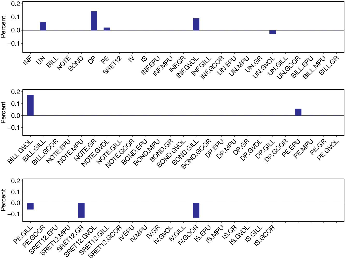

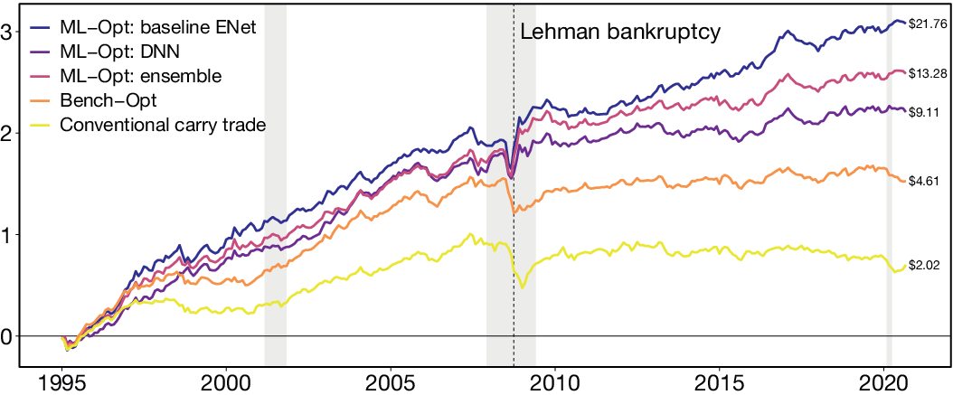


 Open access

