


I. Introduction
The U.S. banking sector is among the most heavily regulated industries and plays a crucial role in economic development (King and Levine (Reference King and Levine1993a), Rajan and Zingales (Reference Rajan and Zingales1998), Peek and Rosengren (Reference Peek and Rosengren2000), Cetorelli and Gambera (Reference Cetorelli and Gambera2001), and Black and Strahan (Reference Black and Strahan2002)). Recent debate has focused on how regulatory changes impact small banks and reshape the composition of the banking sector, particularly given banks’ heterogeneous lending practices (Petersen and Rajan (Reference Petersen and Rajan1994), Berger, Miller, Petersen, Rajan, and Stein (Reference Berger, Miller, Petersen, Rajan and Stein2005)). This issue has become particularly relevant in light of recent structural shifts in the industry: community banks account for 97% of the decline in the number of U.S. banks over the past 2 decades, and recent bank failures have accelerated deposit outflows from regional to large banks.Footnote 1
We examine this issue in the context of a major regulatory shift: the tightening of anti-money laundering (AML) enforcement beginning in late 2012. That year marked a turning point with multiple regulatory changes and high-profile enforcement actions that substantially increased AML enforcement intensity in the U.S. A prominent example is the December 2012 settlement between United States authorities and HSBC, a $1.9 billion fine for money laundering charges, equivalent to 8.7% of the bank’s prior-year pre-tax profits. In response, financial institutions expanded their compliance operations, though the burden was uneven. While AML compliance costs averaged 0.08% of total assets for large banks, it averaged 0.83% for small banks.Footnote 2 This heterogeneity suggests that heightened AML enforcement may have altered the composition of local banking markets, with potential implications for credit supply and local economic outcomes. We analyze these dynamics in this article.
We start by showing that the stricter enforcement of AML regulations altered the composition of the banking sector in areas more exposed to money laundering activities. While all areas operate under the same national enforcement regime, exposure to laundering-related compliance burden varies across locations. We proxy for this exposure using counties designated by the White House Office of National Drug Control Policy as High Intensity Drug Trafficking Areas (HIDTA). In these counties, small banks face disproportionately higher compliance costs.Footnote 3 Consistent with this mechanism, small banks reduce their presence in HIDTA counties, while large banks expand. Importantly, the total number of bank branches remains stable, allowing us to isolate the implications of this compositional shift for bank activity, lending patterns, and real economic outcomes. Our results are robust to a battery of additional tests, such as matching HIDTA and non-HIDTA counties on economic and demographic attributes, using neighboring non-HIDTA counties as controls, using alternative definitions of bank size, excluding strong housing markets, and using alternative measures of exposure to money laundering.
Next, we examine whether the compositional shift toward large banks has implications for credit provision and the real economy. A priori, the effects on credit supply are ambiguous. The loss of small banks may harm the local economy, particularly smaller firms that rely on relationship lending, considering that small banks have advantages in collecting and processing soft information and can lend to otherwise underserved borrowers (Petersen and Rajan (Reference Petersen and Rajan2002), Stein (Reference Stein2002), Berger et al. (Reference Berger, Miller, Petersen, Rajan and Stein2005), and Mian (Reference Mian2006)). Additionally, large banks may reallocate deposits across their networks, potentially reducing local credit availability (Gilje, Loutskina, and Strahan (Reference Gilje, Loutskina and Strahan2016)). On the other hand, large banks may expand local credit through internal capital markets, standardized lending technologies, and government-supported programs such as the Community Reinvestment Act (CRA) and Small Business Administration (SBA) lending, due to their greater scale and heightened regulatory expectations (Stein (Reference Stein1997), (Reference Stein2002), Calomiris and Haber (Reference Calomiris and Haber2015)). Large banks might also access more rigorous risk management and compliance systems, allowing them to serve a broader customer base.Footnote 4 Further, large banks may be less prone to sanctions, consistent with the “too big to jail” hypothesis, potentially enabling them to serve higher-risk customers previously excluded from banking services.Footnote 5
We find that large banks increase lending activity in counties exposed to heightened money laundering activity, effectively compensating for the reduction in credit supply by small banks. This expansion concentrates on lending to small firms and households through standardized government-supported programs and secured credit channels. Specifically, large banks increase the number of CRA loans to small firms by 14%, primarily through small loans. SBA lending increases by 7%, and secured household lending rises by 14% to 20%, depending on loan purpose. Loan volumes show a similar pattern: CRA lending to small firms increases by 14%, SBA lending rises by 40%, and secured household lending grows by 33% to 50%. These findings are consistent with large banks having a comparative advantage in hard-information-based lending, where underwriting can be centralized and standardized (Stein (Reference Stein2002), (Reference Stein, Constantinides, Harris and Stulz2003)).
We then examine county-level lending activity to assess how the shift in bank composition affects credit availability within a county. We find no significant differential effect on the total number and volume of loans under the CRA or SBA programs. Similarly, for mortgage lending, we do not find statistically significant effects on lending for home purchases and refinancing, although we observe an increase in home improvement loans. Overall, our evidence suggests that the expansion of lending by large banks occurs alongside the decline in small-bank activity, without a significant differential change in county-level credit supply. Our results indicate that, in our setting, the lower ability of large banks to process soft information does not result in lower access to credit. Large banks increase credit supply through standardized lending channels, specifically through government-supported programs such as CRA and SBA loans, as well as secured household lending, where collateral mitigates potential losses.Footnote 6
Next, we explore the effects of the compositional shift on real economic outcomes. We document a relative increase in the number of establishments, primarily small businesses, in impacted counties, consistent with Beck and Demirgüç-Kunt (Reference Beck and Demirgüç-Kunt2006) and Adelino, Schoar, and Severino (Reference Adelino, Schoar and Severino2015), who point to the importance of bank lending and collateralized lending for small business growth. We also find relative increases in the number of establishments, employment, and wages for non-tradable sector firms, supporting a household demand channel (Mian, Sufi, and Verner (Reference Mian, Sufi and Verner2020)). These results suggest that, while overall lending volume remains relatively unchanged in these counties, differences in lending practices between large and small banks impact local economic activity. When we focus on small businesses, we find that the effects are stronger in counties with smaller banking markets, consistent with the role of large banks’ internal capital markets in reallocating lending capacity across markets (Stein (Reference Stein1997), (Reference Stein2002), Mian et al. (Reference Mian, Sufi and Verner2020)). We do not find that distance to large banks’ headquarters affects small businesses’ outcomes, suggesting that geographic proximity or soft-information frictions are not the primary drivers of our results.
Taken together, these findings are consistent with a mechanism in which real outcomes improve despite little change in aggregate credit because the AML shock altered the composition of local intermediation and potentially its quality. Large banks expanded through standardized, collateralized, and government-supported channels, while the contraction of small banks in HIDTA counties may have disproportionately affected intermediaries with weaker compliance systems or less effective lending practices. This intermediation-quality channel provides a complementary explanation alongside the hard-information lending channel.
We then explore residential real estate prices, which previous studies link to financial services availability (Mian and Sufi (Reference Mian and Sufi2009)). Real estate prices in HIDTA counties increase relatively more than in other counties. Importantly, the effect is more pronounced in lower-income areas within counties more exposed to money laundering activity, suggesting that the shift toward large banks improves conditions in areas likely to benefit more from access to finance.
Finally, we consider several alternative explanations for our findings. First, we examine whether the results are driven by worsening outcomes in non-HIDTA areas. Our evidence does not support this channel. Second, we test whether the expansion of lending by large banks results in changes in lending risk patterns, and find no indication of higher delinquency or default rates following the shift toward large banks. Third, we examine whether our results point to broader non-credit channels. We find no evidence that AML enforcement affects local crime patterns or that the expansion of small businesses is driven by cash-intensive businesses that could be used to facilitate money laundering. Taken together, these tests suggest that our findings are not driven by these alternative mechanisms. In combination with our earlier evidence, this supports the interpretation that AML enforcement primarily imposes disproportionate compliance costs on small banks in HIDTA counties, thereby reshaping the composition of the banking sector through a reallocation of lending toward larger institutions and consistent with improved intermediation.
Our article contributes to the literature on regulation, banking, and economic growth by examining how tightening AML enforcement leads to a plausibly exogenous shift in bank composition from smaller to larger banks, affecting lending patterns and local economic activity.Footnote 7 This setting allows us to examine, in a recent regulatory context, the effects of changing bank composition without confounding factors such as changes in the number of bank branches or governmental, institutional, and measurement differences across states or countries. The closest papers to ours are Huber (Reference Huber2021), who explores how the 1950s consolidation of German banks affected firms and bank managers, and Bord, Ivashina, and Taliaferro (Reference Bord, Ivashina and Taliaferro2021), who explore changes in lender composition following the 2007 real estate price collapse. We contribute by exploiting a novel experiment and showing that large banks’ increased lending fills the void created by small bank contraction, with evidence suggesting positive impacts on small businesses and residential real estate prices.
Our article also contributes to the relatively scant literature on AML enforcement implications. We provide evidence on the effects of AML regulations on the banking sector and real economy by focusing on areas more susceptible to money laundering. To the best of our knowledge, we are the first to systematically examine AML provisions’ impact on the U.S. banking system by focusing on areas prone to high money laundering activity. By contrast, Slutzky, Villamizar-Villegas, and Williams (Reference Slutzky, Villamizar-Villegas and Williams2026) focuses on liquidity shocks following AML regulations in Colombia transmitted via the branching system, Gara, Manaresi, Marchetti, and Marinucci (Reference Gara, Manaresi, Marchetti and Marinucci2024) explores how AML inspections impact suspicious transaction reporting in Italy, and Gao, Pacelli, Schneemeier, and Wu (Reference Gao, Pacelli, Schneemeier and Wu2023) studies banks’ incentives for reporting suspicious activity. To the extent that recent leaks of the so-called FinCEN files characterize AML enforcement tools as ineffective,Footnote 8 our results suggest that AML enforcement may nevertheless affect banking and economic activity through its impact on compliance costs that affect bank composition.
The rest of the article proceeds as follows: Section II discusses the institutional background. Section III describes the data. Section IV describes the empirical design and provides results on the effects of AML on the banking system and real economy. Section V discusses alternative explanations. Section VI concludes.
II. Institutional Background
A. Anti-Money Laundering (AML) Regulation
Due to the negative consequences associated with money laundering—facilitating corruption and distorting resource allocation, among others—governments worldwide have implemented AML policies. In the United States, the first tool introduced was the Bank Secrecy Act of 1970, which was subsequently expanded and amended several times. Following the terrorist attacks of 2001, the U.S. Congress enacted the USA PATRIOT Act, which contained provisions to strengthen existing AML regulations. These included requiring financial institutions to implement customer identification programs, maintain transaction records, and report suspicious activities through Suspicious Activity Reports (SARs).
B. The 2012 Shift in AML Enforcement Intensity
A significant change in U.S. AML enforcement occurred in 2012, when multiple developments reflected a substantial intensification of regulatory scrutiny in the banking sector.
1. Regulatory and Institutional Changes
In early 2012, the Financial Crimes Enforcement Network (FinCEN) mandated electronic filing of SARs by Apr. 1, 2013. That year, FinCEN incorporated a stand-alone Enforcement Division, and regulators began requiring firms to admit wrongdoing in settlements, a marked departure from earlier practice (Brown-Hruska (Reference Brown-Hruska2016)). FinCEN Director Jennifer Shasky Calvery emphasized that “acceptance of responsibility and acknowledgment of the facts is a critical component of corporate responsibility.”
2. High-Profile Enforcement Actions
One of the most salient actions was the fine imposed in December 2012 on HSBC for money laundering charges, amounting to $1.9 billion and equivalent to 8.7% of HSBC’s prior-year pre-tax profits and 1.4% of its market capitalization. Another example was the “death penalty” imposed on First Bank of Delaware in November 2012, when the regional bank was stripped of its charter due to AML failures. The volume of civil money penalties imposed by the Office of the Comptroller of the Currency also increased significantly, as seen in Figure A1, Graph A in the Supplementary Material.
3. Industry-Wide Response
According to the U.S. Government Accountability Office (U.S. Government Accountability Office (2018a), (2018b), (2020)), many banks cited these fines and enforcement changes as reasons for scaling back operations in the U.S. Southwest border region. As discussed in Simons (Reference Simons2013), AML enforcement actions prompted exits by small and regional banks. Moreover, a 2016 NERA report shows that while only half of AML enforcement actions from 2002–2011 involved monetary penalties, approximately 90% did between 2012 and 2015.Footnote 9
4. Compliance Costs and Operational Impact
Banking institutions expanded compliance capacity on an unprecedented scale: by 2013, JPMorgan and HSBC added 4,000 and 3,000 employees to their compliance teams, respectively. JPMorgan and Citibank increased annual regulatory and compliance spending by $1 billion and $2 billion, respectively.Footnote 10
5. Public Salience
The heightened enforcement intensity was accompanied by increased public attention to money laundering. The number of Wall Street Journal articles mentioning money laundering roughly doubled after 2012 (Figure A1, Graph B in the Supplementary Material), suggesting the issue had become more prominent in public discourse.
Taken together, these developments reflect a marked increase in AML enforcement intensity beginning in 2012, which we use as the regulatory shift underpinning our empirical analysis.
C. High Intensity Drug Trafficking Areas
In 1988, the U.S. Congress created the HIDTA program, aimed at reducing drug trafficking and production. The program provides assistance to local enforcement agencies in areas identified as critical drug-trafficking regions. To qualify, a county must meet four criteria: i) be a significant center of illegal drug production, manufacturing, importation, or distribution; ii) have drug-related activities with significant harmful impact locally and nationally; iii) demonstrate commitment of local law enforcement resources; and iv) require significant additional Federal resources.Footnote 11 As of 2025, approximately 23% of all counties were designated as HIDTA. We map the distribution of HIDTA counties as of 2012 in Figure 1.
Figure 1 highlights counties identified by the White House Office of National Drug Control Policy as High Intensity Drug Trafficking Areas (HIDTA) as of 2012.

FIGURE 1 Long description
A geographical map of the United States divided by county borders. Counties designated as High Intensity Drug Trafficking Areas are shaded in dark blue.
* In the West, there is a heavy concentration along the entire Pacific coast and the southern border with Mexico, extending through Southern California, Arizona, and New Mexico.
* In the Northwest, several counties are highlighted in Washington and Oregon.
* In the Southwest and Mountain regions, clusters appear in Utah, Colorado, and Nevada.
* In the Midwest, isolated clusters are visible around major urban centers in Illinois, Michigan, and Ohio.
* In the Northeast, a dense corridor of highlighted counties runs from the Mid-Atlantic through New England, particularly around New York, Pennsylvania, and Massachusetts.
* In the South, there are significant clusters in Florida, along the Gulf Coast, and scattered throughout Texas, Tennessee, and Kentucky.
* The central Great Plains and upper Midwest regions show the lowest density of designated counties.
We compare HIDTA and non-HIDTA counties as of 2010, the closest census year to our shock, in a series of observable characteristics in Table 1. We find that HIDTA counties are generally larger in population, have higher median income, and their population has a higher percentage of individuals with higher education degrees (Panel A). However, establishments per capita, unemployment, general education levels, and poverty rates are similar across county types.

TABLE 1 Long description
Panel A. Demographic Information (2010): Compares Non-H I D T A (N=2,569) and H I D T A (N=573) counties. Key variables include Median income (log) (10.62 vs 10.75), Population (log) (9.94 vs 11.72), and College degree percentage (19.54 vs 26.56). Significant differences are noted in income, population, and education.
Panel B. Comparative Banking Statistics (2012): Compares Non-H I D T A (N=2,580) and H I D T A (N=528) counties. Deposits per capita are 3.43 for Non-H I D T A and 3.49 for H I D T A. Branches per 1,000 capita are 0.44 for Non-H I D T A and 0.30 for H I D T A, showing a significant difference of 0.15. Growth rates for deposits and branches are provided for 1, 2, 3, and 4-year intervals (Delta = 1 to 4).
Panel C. Summary Statistics: Provides Mean, Standard Deviation, Minimum, Median, Maximum, and N for various categories:
- Bank-county level: Deposits (asinh) mean 8.887; Branches (asinh) mean 1.115.
- County level: Deposits (asinh) mean 13.699; Branches (asinh) mean 2.729.
- Bank costs: Compliance costs/assets mean 0.854; General costs/assets mean 12.966.
- C R A lending: Includes loan numbers and amounts for small, medium, and large categories.
- S B A lending: Loans (number) mean 1.761; Loans (amount) mean 10.640.
- H M D A lending: Covers home purchase, improvement, and refinancing.
- Local economic activity: Establishments mean 7.195; Employment mean 9.501; Wages mean 18.593.
- Real estate: Median listing price mean 12.682; Zillow index (all homes) mean 12.348.
- D E A spending: D E A spending (asinh) mean 1.195.
In Panel B, we compare the banking system across HIDTA and non-HIDTA counties as of 2012. While we find differences in the level of deposit volumes and branches per capita, we find no differences in prior growth rates. In addition, consistent with a positive relationship between drug trafficking and money laundering, we find that a larger fraction of SARs is issued in HIDTA counties. In 2012, 74% of SARs were issued in HIDTA counties, which account for 53% of bank branches. In the following 3 years, the percentages rose to 80%, 80%, and 78%, respectively.
D. Compliance Costs
Stricter AML enforcement may affect bank composition through disproportional compliance costs imposed on small banks, given that such banks face higher overhead investment and smaller economies of scale. We provide evidence that compliance costs are relatively higher for smaller banks and particularly in HIDTA counties by employing proprietary data compiled by the Conference of State Bank Supervisors (CSBS) and the state banking commissioners via its annual National Survey of Community Banks. In 2015, the first year for which we have data, more than 600 banks responded to the survey.
Among other questions, bankers were asked to “identify the compliance costs they incurred in personnel, data processing, legal services, accounting and auditing, and consulting.” Using bank-level data, we compare compliance costs across banks with different levels of exposure to HIDTA counties.Footnote 12 First, in Figure 2 we plot the compliance costs as a fraction of assets for banks that are highly exposed to HIDTA counties (share of deposits in HIDTA counties above 50%) and those that are less exposed to HIDTA counties in Graph A, and for small and large banks (assets above/below the median value across banks) in Graph B. We find that compliance costs are significantly higher for banks more exposed to HIDTA counties and for smaller banks.Footnote 13
Figure 2 shows the overall compliance costs for banks more (less) exposed to HIDTA counties (Graph A) and for small and large banks (Graph B). Banks that source more than 50% of their deposits from HIDTA counties are categorized as HIDTA. Banks with assets above the median value for all banks are categorized as large. The data are from the Conference of State Bank Supervisors’ 2015 National Survey of Community Banks.

FIGURE 2 Long description
The image consists of two vertical bar charts arranged one above the other.
Graph A (Top Panel):
* The y-axis is labeled Compliance Costs over Assets with numerical increments from 1.5 to 2.
* The x-axis has two categories: Non-H I D T A and H I D T A.
* The Non-H I D T A bar reaches approximately 1.74.
* The H I D T A bar is higher, reaching approximately 1.88.
Graph B (Bottom Panel):
* The y-axis is labeled Compliance Costs over Assets with numerical increments from 0 to 2.
* The x-axis has two categories: Small and Large.
* The Small bank bar reaches approximately 2.2.
* The Large bank bar is significantly lower, reaching approximately 1.25.
Moreover, we exploit the richness of the data to study how exposure to HIDTA counties affects compliance costs relative to bank size by estimating:

where Compliance Cost
$ {}_b $
 is the cost of compliance for Bank
$ b $
 scaled by total assets, Exposure HIDTA
$ {}_b $
 is the share of deposits held in HIDTA counties, and Bank Size
$ {}_b $
 is the inverse hyperbolic sine transformation of deposit volume to proxy for a bank’s size. We present the results in Table 2, which show that bank size is negatively correlated with compliance costs, while HIDTA exposure is positively correlated. The interaction term is negative, indicating that compliance costs in HIDTA counties are relatively lower for larger banks. These results suggest that compliance costs in counties more exposed to money laundering are higher and even more pronounced for smaller banks. A 1-standard-deviation increase in HIDTA deposit share translates into a 0.73 percentage point (1.644
$ \times $
 0.448) increase in compliance costs. To put this in perspective, LexisNexis Risk Solutions (2018) estimated that U.S. financial institutions spend roughly $25.3 billion annually on AML compliance; our estimates suggest that heightened HIDTA exposure could raise these costs significantly, with the burden falling disproportionately on smaller banks. For robustness, column 4 normalizes compliance costs by deposits instead of assets, with comparable results. As a placebo test in columns 5 and 6, we examine whether general expenses (not related to compliance) exhibit similar patterns and find that they do not.

TABLE 2 Long description
The table consists of six columns of regression results. Columns 1 through 3 measure Compliance Costs normalized by Assets. Column 4 measures Compliance Costs normalized by Deposits. Column 5 measures General Costs normalized by Assets. Column 6 measures General Costs normalized by Deposits.
Key findings by row:
* Bank size: Shows a consistent negative correlation with compliance costs across columns 1 through 4, with coefficients ranging from minus 0.138 to minus 0.182, all significant at the 1 percent level. General costs in columns 5 and 6 also show negative coefficients but are not statistically significant.
* Exposure H I D T A: Shows a positive correlation with compliance costs. In column 2, the coefficient is 0.176 (1 percent significance). In columns 3 and 4, coefficients are 1.406 and 1.644 respectively (5 percent significance).
* Bank size times exposure H I D T A: This interaction term shows negative coefficients in columns 3 and 4 (minus 0.096 and minus 0.112), significant at the 5 percent and 10 percent levels respectively.
* N (Sample size): 498 for compliance cost models and 509 for general cost models.
* Adjusted R-squared: Ranges from 0.114 to 0.138 for compliance costs, and 0.028 to 0.032 for general costs.
III. Data
In this section, we describe the multiple data sets used in our study of the effect of stricter enforcement of AML regulations on the banking sector and the real economy. We provide summary statistics of the variables used in our study in Panel C of Table 1.
A. Deposits and Bank Branches
Our first data source is the Federal Deposit Insurance Corporation’s (FDIC) summary of deposits, containing yearly information on deposits at the bank-branch level. We collect data from 2010 to 2016 for all brick-and-mortar bank branches in the 50 U.S. states and the District of Columbia, yielding approximately 85,800 bank-branch observations per year for close to 8000 different banks.Footnote 14
B. Money Laundering Activity
Our second source of data measures exposure to money laundering activities, and in particular to those originating in the production and distribution of illegal drugs. We collect data on counties identified by the White House Office of National Drug Control Policy (ONDCP) as HIDTA. We remove counties added after 2012 to mitigate look-ahead bias. For robustness, we construct an alternative measure of exposure using the distance between a county and the closest Drug Enforcement Administration (DEA) office, assuming regional DEA offices are established in areas more exposed to illegal drug production and distribution. We also use distance to DOJ offices for robustness.Footnote 15
C. CRA Lending
We collect data on lending to small businesses under the CRA from the Federal Financial Institutions Examination Council (FFIEC). The CRA, enacted in 1977, encourages financial institutions to lend to low- and moderate-income borrowers in their operating communities. While institutions lack specific targets, they are overseen by the OCC, FDIC, and FRB, who rate their performance. The program’s volume is substantial: in 2021 alone, reporting banks lent $371 billion under CRA, a considerable amount given that total commercial and industrial loans by all commercial banks are around $2.5 trillion.Footnote 16 We obtain county-level data from 2010 to 2016 on the number and volume of loans to small businesses (annual revenues below $1 million).
D. SBA and HMDA Lending
We collect data on loans issued under the SBA 7(a) Loan Guarantee program, where the SBA partially guarantees loans to encourage lending to small businesses that might otherwise not be funded. We collect data on more than 370,000 loans issued between 2010 and 2016. We also collect mortgage data from the Home Mortgage Disclosure Act (HMDA), obtaining lending data on mortgages for purchases, home improvement, and refinancing for each reporting financial institution at the county-year level between 2010 and 2016. Our database contains information on more than 8,000 lenders in over 3,000 counties.Footnote 17
E. Economic Outcomes
Our real economic outcome measures come from the Bureau of Labor Statistics on employment, wages, and the number of active establishments through the Quarterly Census of Employment and Wages. We obtain quarterly and yearly information at the county level with different aggregation levels, including employer type (government or private) and NAICS sector. We also obtain data from the County Business Patterns series to study firms of different sizes by number of employees.
F. Real Estate
We obtain real estate price data from Zillow at the zip code level, including statistics such as median listing price and median listing price per square foot.
G. Loan Performance and Underwriting
Our first source of data is the Consumer Financial Protection Bureau (CFPB), which publishes data on delinquency rates using a nationally representative, 5% sample of all outstanding, closed-end, first-lien, 1–4 family residential mortgages. The data is provided at the county-month-year level for approximately 470 counties, out of which 268 were designated as HIDTA in 2012. Our second source is CoreLogic, which provides loan-level data, allowing us to explore outcomes for loans originated at different points in time. Our data are restricted to loans originated in the State of Maryland, which includes 10 HIDTA and 14 non-HIDTA counties.Footnote 18
H. Crime
We collect crime data from the FBI’s Uniform Crime Reporting (UCR) Program, which includes information on the number of crimes for different criminal activities, such as murder, manslaughter, rape, robbery, assault, and theft.
IV. Empirical Analysis
We study the effects of tighter AML enforcement using a difference-in-differences framework, exploiting cross-sectional differences in money laundering exposure and the timing of the 2012 AML enforcement tightening. Later, we extend our tests to incorporate a third difference for cross-sectional differences in bank characteristics. A key assumption in our study is that there are no pre-trends: the banking sectors in treated (HIDTA) and control (non-HIDTA) counties should exhibit common trends before the shock. In Panel B of Table 1, we show that both bank deposits’ and bank branches’ prior growth is comparable in treated and control counties as of 2012.
A. Bank Branches and Deposits Volume
We start by examining the effect of tightening AML enforcement on the number of branches and deposit volumes using the following specification:

where
$ {y}_{c,s,t} $
 is one of our outcomes of interest (inverse hyperbolic sine transformation of the number of branches or volume of deposits), Post
$ {}_t $
 is an indicator equal to 1 from 2013 onward, HIDTA
$ {}_c $
 is an indicator for counties designated as HIDTA as of 2012, and
$ {\gamma}_c $
 are county-level controls (unemployment rate, log population, log median income) fixed at pre-period (2011) values and interacted with the Post
$ {}_t $
 indicator to control for differential shocks across counties with varying economic and demographic profiles.Footnote
19 In addition, we control for spending by the DEA at the county-year level to account for initiatives that might have affected counties differently, using data obtained from www.usaspending.gov.Footnote
20 We include county (
$ {\alpha}_c $
 ) and state-year (
$ {\alpha}_{s,t} $
 ) fixed effects to account for time-invariant characteristics of the banking sector at the county level and for state-specific shocks.
We present the results in Table 3. The coefficients in columns 1 and 2 show that the total number of branches in HIDTA counties does not decline relatively more compared to other counties following the shift in AML enforcement. More specifically, the coefficient for Post × HIDTA is statistically and economically indistinguishable from 0 in both specifications. This evidence is in line with the graphical evidence presented in Graph A of Figure 3, which shows that the total number of branches follows similar patterns in both HIDTA and non-HIDTA counties. On the other hand, we find that the positive coefficient for the volume of deposits (columns 3 and 4) is economically and statistically significant. These results indicate that the volume of deposits increases in HIDTA counties relative to non-HIDTA counties following stricter AML enforcement. For robustness, we present the estimations excluding county-level controls in Table A2 in the Supplementary Material, and find results that are comparable to the baseline evidence.

TABLE 3 Long description
The table consists of four columns of regression results. Columns 1 and 2 use Branches as the dependent variable, while columns 3 and 4 use Deposits.
* The primary independent variable is the interaction term Post times H I D T A.
* For Branches (Column 1): Coefficient is 0.004 with a t-statistic of 1.09.
* For Branches (Column 2): Coefficient is 0.003 with a t-statistic of 0.71.
* For Deposits (Column 3): Coefficient is 0.026, significant at the 5 percent level, with a t-statistic of 2.47.
* For Deposits (Column 4): Coefficient is 0.020, significant at the 10 percent level, with a t-statistic of 2.01.
Summary statistics and fixed effects:
* N is 21,745 for columns 1 and 3, and 21,738 for columns 2 and 4.
* Adjusted R-squared ranges from 0.996 to 0.997.
* County Fixed Effects (F E) and Controls are included in all columns.
* Year F E is included in columns 1 and 3, while State times Year F E is included in columns 2 and 4.
Figure 3 shows the evolution of the total number of bank branches in HIDTA and non-HIDTA counties between 2006 and 2018 (Graph A) and the share of branches of large banks in HIDTA and non-HIDTA counties (Graph B). Large banks are defined as those that are in the top 1% in terms of volume of deposits and that have at least 100 branches across the United States. The data on bank branches are from the Summary of Deposits, reported by the FDIC. HIDTA counties are those identified by the White House Office of National Drug Control Policy as of 2012.

FIGURE 3 Long description
A two-panel vertical layout of line graphs.
Top Graph: Total number of bank branches.
- The X-axis represents Year from 2006 to 2018.
- The Y-axis represents Branches from 35,000 to 50,000.
- A vertical red line is positioned between 2012 and 2013.
- The H I D T A line (red) starts at 45,000 in 2006, peaks near 48,000 in 2008-2009, and steadily declines to approximately 44,000 by 2018.
- The non-H I D T A line (blue) starts at 40,000, peaks near 41,000 in 2008-2009, and declines to approximately 36,000 by 2018.
Bottom Graph: Share of large bank branches.
- The X-axis represents Year from 2006 to 2018.
- The left Y-axis represents H I D T A percent from 56 to 64.
- The right Y-axis represents non-H I D T A percent from 35 to 39.
- A vertical red line is positioned between 2012 and 2013.
- The H I D T A line (blue) shows a steep upward trend from 56 percent in 2006 to nearly 63 percent in 2018.
- The non-H I D T A line (red) shows an upward trend from 34 percent in 2006 to a peak of 37 percent in 2013, followed by a slight decline to 36 percent by 2018.
B. Composition of Bank Branches and Deposit Volumes
Next, we study how stricter AML enforcement impacts large and small banks operating within affected counties. In particular, given the heterogeneous compliance costs shown in the previous section, this change likely impacts the composition of the banking sector. We expand our previous specification in the following way:

In this specification, the unit of observation is the bank-county-year.
$ {y}_{b,c,s,t} $
 is one of the outcomes of interest (inverse hyperbolic sine transformation of the number of branches, volume of deposits). The indicator variable
$ {Large}_b $
 is set to 1 for banks in the top 1% in terms of deposits and that have at least 100 branches across the United States, thus excluding financial institutions associated with credit cards or investment banks. We include multiple sets of fixed effects. In our stricter specification, we include bank-county fixed effects (
$ {\alpha}_{b,c} $
 ) to control for time-invariant characteristics of the operations of a bank in each county, bank-year fixed effects (
$ {\alpha}_{b,t} $
 ) to control for general shocks to each bank, and county-year fixed effects (
$ {\alpha}_{c,t} $
 ) to control for local shocks. Thus, in this tight specification, both local and general time-varying factors that may affect banking activity are controlled for, mitigating concerns about county-level time-varying economic or demographic factors that might affect the findings. Standard errors are double-clustered at the county and year level.
We present the results in Table 4. For the number of branches (columns 1–3), we find that small banks reduce their presence in HIDTA counties relative to non-HIDTA counties following the stricter enforcement of AML regulations, as reflected by the negative coefficient on Post × HIDTA. The triple interaction term is positive and significant, indicating that large banks increase their presence in HIDTA counties more than in non-HIDTA counties following the shock. Notably, this coefficient is statistically significant in all specifications, including column 3 where we include a strict set of fixed effects. This finding is consistent with the graphical evidence observed in Graph B of Figure 3, where we plot the raw evolution of the share of branches by large banks in HIDTA versus non-HIDTA counties. The presence of large banks in both types of counties follows a similar pattern between 2006 and 2012. However, following the tightening of the enforcement of AML regulations, large banks increase their presence in HIDTA counties vis-à-vis non-HIDTA counties.

TABLE 4 Long description
The table consists of six columns. Columns 1 through 3 use Branches as the dependent variable, and columns 4 through 6 use Deposits.
Key independent variables and their coefficients include:
* Post times H I D T A: Negative coefficients across columns 1, 2, 4, and 5, ranging from -0.026 to -0.392, significant at the 5% level.
* H I D T A times large: Positive coefficients in column 1 (0.630) and column 4 (0.805), significant at the 1% level.
* Post times large: Positive coefficients in column 1 (0.026), column 4 (0.660), and column 5 (0.753), significant at the 1% or 10% levels.
* Post times H I D T A times large: Positive and significant across all columns, ranging from 0.033 to 0.676.
Statistical summary data:
* N (Observations): Ranges from 202,784 to 232,571.
* Adjusted R-squared: Ranges from 0.575 to 0.946.
Fixed Effects (F E) and Controls:
* Columns 1 and 4 include County, Bank, and Year F E.
* Columns 2 and 5 include State times year F E and Bank times county F E.
* Columns 3 and 6 include Bank times year, County times year, and Bank times county F E.
* Controls are included in columns 1, 2, 4, and 5.
These findings are consistent with the idea that higher compliance costs for small banks contributed to a shift toward large banks both at the extensive and intensive margin (branches and deposits, respectively) in the areas that are more prone to money laundering activity. For completeness, we plot the year-by-year coefficient for the triple interaction term in Figure 4, where we observe that the response is immediate and materializes fully 2 years after stricter enforcement of AML regulations. For deposit volumes (columns 4–6), we find a similar pattern. Small banks’ deposit volumes decline in HIDTA counties, while large banks’ deposit volumes increase. The triple interaction term is positive and statistically significant, indicating that large banks capture a larger share of deposits in HIDTA counties following the enforcement shift.
Figure 4 shows the dynamic coefficients of a regression of the inverse hyperbolic sine transformation of the number of branches that large banks have in HIDTA counties across time. Large banks are defined as those that are in the top 1% in terms of volume of deposits and that have at least 100 branches across the United States. The data on bank branches are from the Summary of Deposits as reported by the FDIC. HIDTA counties are those identified by the White House Office of National Drug Control Policy by 2012.

FIGURE 4 Long description
A line graph where the vertical Y axis is labeled Estimated coefficient and ranges from minus 0.02 to 0.06 in increments of 0.02. A horizontal red reference line is drawn at 0. The horizontal X axis contains integer labels from minus 2 to 4. The data is represented by seven blue circular points with vertical dashed error bars.
* At X equals minus 2, the point is slightly above 0 with error bars crossing the 0 line.
* At X equals minus 1, the point is slightly below 0 with error bars crossing the 0 line.
* At X equals 0, the point sits exactly on the 0 line with no visible error bars.
* At X equals 1, the point rises to approximately 0.01 with error bars entirely above the 0 line.
* At X equals 2, the point jumps to approximately 0.04 with error bars between 0.025 and 0.055.
* At X equals 3, the point drops slightly to approximately 0.03 with error bars between 0.015 and 0.05.
* At X equals 4, the point rises to its highest level at approximately 0.045 with error bars between 0.025 and 0.065.
We explore several alternative sample specifications in this context. For conciseness, we present the results of the specifications that include the stricter sets of fixed effects in Table 5. Complete tables, including all specifications, are presented in Tables A3–A6 in the Supplementary Material. In Table 5, first, we consider an alternative definition of large banks (assets above $1 billion) in columns 1 and 5, and find similar results. Next, we match each HIDTA county with the most similar non-HIDTA county based on income, population, and education and find broadly consistent results in columns 2 and 6. We further repeat our analysis focusing on non-HIDTA counties neighboring HIDTA counties as controls in columns 3 and 7 and find evidence supporting our baseline findings. We also consider the possibility that our results respond to the increased activity by large banks in strong housing markets (Chakraborty, Goldstein, and MacKinlay (Reference Chakraborty, Goldstein and MacKinlay2018)). To address this issue, we use the Federal Housing Finance Agency’s data on House Price Indexes (HPI) and construct a list of county-years for which the HPI index’s appreciation over the previous 5 years is in the top decile, equivalent to an increase of over 17%. As reported in columns 4 and 8, we find that our results hold when we exclude these markets.

TABLE 5 Long description
The table is divided into two sections: Panel A and Panel B.
Panel A: Alternative Sample Specifications.
This panel includes 8 columns. Columns 1 through 4 measure Branches, and columns 5 through 8 measure Deposits.
* The primary row, Post times H I D T A times large, shows coefficients for Alt. Bank Size (0.094 and 0.936), Matched Sample (0.023 and 0.211), Neighboring Non-H I D T A (0.038 and 0.278), and Excluding Strong Housing Markets (0.030 and 0.276).
* Sample sizes N range from 41,735 to 202,784.
* Adjusted R-squared values range from 0.926 to 0.953.
* All specifications include Bank times year, County times year, and Bank times county Fixed Effects (F E).
Panel B: Alternative Measures of Money Laundering Exposure.
This panel includes 10 columns. Columns 1 through 5 measure Branches, and columns 6 through 10 measure Deposits.
* The primary row, Post times measure times large, shows coefficients for D E A Proximity (0.044 and 0.448), D E A Distance (0.211 and 1.599), D O J Proximity (0.016 and 0.284), D O J Distance (0.477 and 5.529), and Enforcement Intensity Index (0.021 and 0.226).
* Sample sizes N are either 201,693 or 202,784.
* Adjusted R-squared values are 0.949 for Branches and 0.930 for Deposits.
* All specifications include Bank times year, County times year, and Bank times county F E.
A natural question is why large banks did not expand earlier in these markets. Our interpretation is that the enforcement shift changed relative profitability rather than revealing newly profitable markets. Before the shock, incumbent small banks benefited from local relationships, established branch networks, and customer-specific knowledge, while large banks faced entry and organizational frictions. Heightened AML enforcement raised fixed and quasi-fixed compliance costs disproportionately for small banks in high-exposure counties, weakening these incumbent advantages and making expansion by large banks relatively more attractive. This interpretation is consistent with theories emphasizing the role of organizational structure, soft information, and internal capital markets in shaping lending behavior across bank types (Stein (Reference Stein1997), (Reference Stein2002), (Reference Stein, Constantinides, Harris and Stulz2003), Berger et al. (Reference Berger, Miller, Petersen, Rajan and Stein2005)).
We also explore whether our results can be driven by banks’ failures and acquisitions. Figure A2 in the Supplementary Material shows that branches in HIDTA counties and those in non-HIDTA counties follow similar patterns in terms of acquisitions (Graph A) and failures (Graph B), thus mitigating the concern that differential trends drive our results. In a placebo test, we randomly designate 17% of the counties as HIDTA—the proportion of counties designated as HIDTA as of 2012—and find small and statistically insignificant effects (Table A7 in the Supplementary Material), suggesting our results are not driven by spurious correlation. Our results are also robust to using natural logarithms for transformations, as shown in Table A8 in the Supplementary Material. In addition, Table A9 in the Supplementary Material provides results using a measure developed by Törnqvist, Vartia, and Vartia (Reference Törnqvist, Vartia and Vartia1985) for relative change that accommodates entry and exit, as in Choi, Goldschlag, Haltiwanger, and Kim (Reference Choi, Goldschlag, Haltiwanger and Kim2023), given that a key aspect in our analysis is the change in the composition of banks. We find similar results.
As additional robustness tests, we employ alternative measures of money laundering in Panel B of Table 5 with the stricter set of fixed effects and provide results with alternative fixed effects in Tables A10 and A11 in the Supplementary Material. Given that the DEA likely locates regional offices in areas with greater exposure to drug production and trafficking, we construct two additional county-level exposure measures: i) an indicator for counties within 50 miles of a DEA office and ii) a continuous measure of proximity to the nearest DEA office.Footnote 21 For consistency and ease of interpretation, proximity is defined as the difference between the maximum distance from any county to a DEA office (approximately 2,600 miles, corresponding to Aleutians West, Alaska) and each county’s distance to the nearest office. Under this transformation, counties hosting a DEA office receive the highest value, while more distant counties receive lower values. Figure A3, Graph A, in the Supplementary Material provides a graphical representation of this measure. We run a similar exercise using proximity to DOJ offices, given that it provides a measure of enforcement intensity, since counties closer to DOJ offices are more likely to receive federal attention and resources. Figure A3, Graph B, in the Supplementary Material provides a graphical representation of this measure. We provide the results of these alternative specifications in columns 1–4 and 6–9 in Panel B of Table 5, where we find results that are consistent with the ones in Table 4.
In addition, we combine the information on the location of DEA and DOJ offices and construct an intensity index ranging from 0 to 3 that considers i) whether the county has been designated as HIDTA, ii) the presence of a DEA office within 50 miles, and iii) the presence of a DOJ office within 50 miles. We map this index in Figure A3, Graph C in the Supplementary Material. The results in columns 5 and 10 of Table 5, Panel B, are largely consistent with the baseline findings. More specifically, we find that small banks reduce their operations by more in counties with higher treatment intensity, while large banks expand operations in these counties. Specifications with alternative fixed effects are in Table A10, Panel C in the Supplementary Material.
We also examine whether pre-shock (2011) bank characteristics were associated with differential exit rates among small banks following the 2012 AML enforcement shift. Figure A7 in the Supplementary Material reports interaction coefficients from complementary log–log and logit models relating post-shock exit probabilities to pre-shock bank characteristics. Across specifications, we find little evidence that exit rates varied systematically with banks’ pre-shock profitability, capitalization, liquidity, funding structure, or labor-intensity measures. Overall, the results suggest limited heterogeneity in the exit response across banks based on the observable pre-shock characteristics available in our data. At the same time, our analysis cannot account for a range of potentially important but unobserved dimensions—such as managerial quality, compliance practices, organizational capacity, or risk-management systems—that may have influenced banks’ ability to absorb the regulatory shock.
C. Lending by Large Banks
A priori, it is unclear how the shifting bank composition from smaller to larger banks would affect access to credit. On the one hand, this change could negatively impact credit. For instance, given that larger banks have a broader network of branches, funds sourced in these counties could be lent in other areas. Moreover, since large banks could be at a disadvantage in terms of processing soft information, it could lead to a reduction in lending to small businesses. On the other hand, large banks may benefit from greater diversification, access to internal capital markets, and the ability to spread fixed costs across a broader lending portfolio, enabling them to expand credit in local economies, particularly where banking markets are thin. In addition, lending by large banks under programs such as the CRA or the SBA Act could increase access to finance, particularly for smaller firms and lower-income communities. Furthermore, if large banks are able to implement more effective compliance risk systems, these banks could screen and monitor clients more efficiently and thus broaden access to finance for a wider group. Alternatively, if larger banks are less prone to sanctions (too big to jail), these banks might be willing to operate with riskier customers and, therefore, expand operations in higher-risk counties.
We examine how the shift toward large banks affects bank lending with the following specification:

where
$ {y}_{b,c,s,t} $
 is one of the outcomes of interest (inverse hyperbolic sine transformation of the number or volume of loans),
$ {\alpha}_{c,t} $
 is a county-year fixed effect,
$ {\alpha}_{b,t} $
 is a bank-year fixed effect, and
$ {\alpha}_{b,c} $
 is a bank-county fixed effect. This specification includes granular fixed effects that absorb bank-specific shocks, county-specific shocks, and time-invariant bank-county characteristics. To account for the presence of banks that stop making certain types of loans to small businesses, we balance each panel by setting missing observations to 0.
We focus on one type of lending at a time and present the results in Table 6. When analyzing CRA loans, we find that large banks relatively increase the number of loans in HIDTA counties following their expanded presence (Panel A). These results are mainly driven by small CRA loans (face value below $100,000), with no significant effects on medium and large loans.

TABLE 6 Long description
The table is divided into three panels: Panel A, Panel B, and Panel C.
Panel A: Community Reinvestment Act (C R A) Lending.
Columns 1 through 4 represent the number of loans (N) for All, Small, Medium, and Large categories. Columns 5 through 8 represent loan volume (A) for the same categories.
- Row ‘Post times H I D T A times large’ shows coefficients: 0.141* (t-stat 2.16), 0.143* (2.18), 0.006 (0.39), 0.001 (0.07), 0.141 (1.59), 0.096 (1.13), 0.090 (1.40), and 0.097 (1.89).
- Observations (N) are 925,822 across all columns.
- Adjusted R-squared values range from 0.648 to 0.883.
- Fixed effects (F E) for Bank times year, County times year, and Bank times county are all marked ‘Yes’.
Panel B: Small Business Administration (S B A) Lending.
Columns include Loans (N), Loans (A), and S B A Guaranteed.
- Row ‘Post times H I D T A times large’ shows coefficients: 0.073* (2.14), 0.403 (1.85), and 0.378 (1.84).
- Observations (N) are 193,882.
- Adjusted R-squared values are 0.659, 0.399, and 0.399.
- All Fixed Effects are marked ‘Yes’.
Panel C: Home Mortgage Disclosure Act (H M D A) Lending.
Columns 1 through 3 represent the number of loans (N) for Purchase, Improvement, and Refinancing. Columns 4 through 6 represent loan volume (A) for the same categories.
- Row ‘Post times H I D T A times Large’ shows coefficients: 0.145** (3.63), 0.199*** (4.25), 0.146** (3.54), 0.423** (3.40), 0.506** (3.19), and 0.334* (2.15).
- Observations (N) vary: 2,704,079 (Purch.), 850,061 (Impr.), and 3,477,755 (Refi.).
- Adjusted R-squared values range from 0.644 to 0.796.
- All Fixed Effects are marked ‘Yes’.
The results in Panel B show that large banks increase relatively the number of SBA loans, amount of loans, and receive a proportional increase in guarantee amounts, though the last two coefficients are only statistically significant at the 11% level.Footnote 22 The results in Panel C show that large banks increase HMDA lending for all purposes (home purchases, improvement, and refinancing) in HIDTA counties, both in number and volume of loans. The triple interaction term is large, positive, and statistically significant for numbers and amounts across loan purposes.
Overall, results across all loan types (CRA, SBA, and mortgages) suggest that following the compositional shift toward large banks, large banks increase lending to small firms under government-supported and guaranteed programs and also increase secured lending to households where collateral can compensate for potential losses. The increase in secured mortgage lending by large banks is consistent with the view that they have a comparative advantage in hard-information-based lending, where soft information is less critical, and underwriting can be centralized and standardized. A similar argument applies to SBA lending, which is government-guaranteed and relies heavily on standardized criteria, reducing the importance of relationship-specific soft information. These findings align with theories suggesting that hierarchical organizations have a comparative advantage in processing standardized hard information through centralized decision structures (Stein (Reference Stein2002), (Reference Stein, Constantinides, Harris and Stulz2003)).
D. Lending Across Banks
While we observe increased lending by large banks following the change in the composition of the banking sector, it is unclear whether this increase under-, over-, or just compensates for the reduction in small bank activity, and how this change affects total credit supplied to the local economy. To explore this, we aggregate lending across banks at the county-year level for each program and estimate equation (2) with aggregate lending as the outcome.
We present the results in Table 7. The coefficients in Panel A (CRA) suggest that there are no significant effects on the total number of loans (total, small, medium, or large) or the volume of loans. This is in line with the idea that the expansion of credit by large banks compensates for the decline in activity by small banks. Similarly, Panel B (SBA loans) shows that there are no changes in SBA credit supplied at the county level, with the number, amount, and guarantees showing no significant changes. Panel C (HMDA loans) finds mostly no impact on the total number or volume of loans, except for home improvement loans (columns 2 and 5), where we find a significant increase.

TABLE 7 Long description
The table is divided into three panels: Panel A for Community Reinvestment Act (C R A) lending, Panel B for Small Business Administration (S B A) lending, and Panel C for Home Mortgage Disclosure Act (H M D A) lending.
* Panel A: Community Reinvestment Act (C R A) Lending
This panel has 8 columns. Columns 1 to 4 represent the number of loans (N) for All, Small, Medium, and Large categories. Columns 5 to 8 represent the volume of loans (A) for the same categories. The primary row is Post times H I D T A. Significant results are found for Small loans (N) with a coefficient of 0.116 (t-statistic 1.97). All columns have N = 21,140 and include County F E, State times year F E, and Controls.
* Panel B: Small Business Administration (S B A) Lending
This panel has 3 columns: Loans (N), Loans (A), and S B A Guaranteed amount. The Post times H I D T A coefficients are 0.038, -0.009, and -0.002 respectively, none of which are marked as statistically significant. N = 21,140 for all columns with all fixed effects and controls applied.
* Panel C: Home Mortgage Disclosure Act (H M D A) Lending
This panel has 6 columns. Columns 1 to 3 represent the number of loans (N) for Purchase, Improvement, and Refinancing. Columns 4 to 6 represent the volume of loans (A) for the same categories. Significant positive results are found for Improvement loans: 0.085 (t-statistic 2.95) for number and 0.107 (t-statistic 2.40) for volume. N = 21,924 for all columns with all fixed effects and controls applied.
While our earlier results show marked shifts in branch and deposit composition toward large banks, we find limited evidence of corresponding changes in the overall volume of lending at the county level. The results suggest a reallocation of lending across institutions. Strengthened AML enforcement, and the resulting increase in compliance costs, appear to have shifted lending activity from small banks toward large banks with no significant relative change in total credit supply at the county level.
E. Real Economic Effects
The absence of a strong effect on aggregate county-level credit does not imply that the change in bank composition is economically neutral. A key implication of our setting is that local outcomes may respond not only to the quantity of credit, but also to the identity of the intermediaries supplying it and the terms or channels through which that credit is delivered. In our context, the expansion of large banks is concentrated in standardized, government-supported, and secured lending channels. At the same time, in counties more exposed to laundering activity, the contraction of small banks may disproportionately affect incumbents whose intermediation was less efficient or whose compliance systems were weaker. These two forces together provide a mechanism through which relatively unchanged aggregate credit can still be associated with changes in real outcomes.
1. Establishments, Employment, and Wages
We analyze the effect of changing bank composition on employment, wages, and number of establishments using information from the Quarterly Census of Employment and Wages (QCEW) and CBP at three aggregation levels. First, at the county-year level, we estimate the effects on total outcomes using a specification similar to that of equation (2). Second, we analyze effects on firms of different sizes, following Guiso et al. (Reference Guiso, Sapienza and Zingales2004), who suggest that local finance matters more for smaller firms. Third, following Mian et al. (Reference Mian, Sufi and Verner2020), we analyze the role of credit supply in tradable and non-tradable sectors separately to shed light on the economic forces behind our results.
The results in Table 8, Panel A, show a small but positive relative effect on the total number of establishments at the county level. Following the compositional change, the total number of establishments in HIDTA counties increases relatively by approximately 1%. We find no significant effect on total employment or wages. We then use CBP data to explore the effect on firms of different sizes. The results in Panel B show that the positive effect on total establishments is driven by small firms, particularly those with fewer than 100 employees. We plot the year-by-year coefficient for the interaction term for small firms in Figure A5 in the Supplementary Material. This finding is consistent with our result that large banks continue providing loans to small firms through CRA and SBA programs and secured lending to households. This aligns with Beck and Demirgüç-Kunt (Reference Beck and Demirgüç-Kunt2006) and Adelino et al. (Reference Adelino, Schoar and Severino2015), which discuss that providing liquidity and financing through secured lending may spur growth in micro and small businesses. Given that small establishments are bank-dependent, our finding suggests that increased large bank presence maintains access to financing for these firms through government programs and secured lending, compensating for the potential lack of soft information processing ability by large banks. We observe a decline in employment and wages for small firms, potentially driven by the increasing number of smaller firms entering with lower initial wages.

TABLE 8 Long description
The table is divided into three panels: Panel A (Overall Sample), Panel B (By Firm Size), and Panel C (By Sector).
Panel A: Overall Sample
* Dependent variables: Establishments (1), Employment (2), and Wages (3).
* Post times H I D T A coefficient: 0.010 super ** (t-stat 2.64) for Establishments; 0.001 (t-stat 0.14) for Employment; -0.029 (t-stat -1.29) for Wages.
* Observations (N): 21,917.
* Adjusted R-squared: 0.999, 0.964, and 0.886 respectively.
* Controls: County F E, State times year F E, and Controls are all marked ‘Yes’.
Panel B: By Firm Size
* Categorized by Micro (<20), Small (20-99), Medium (100-499), and Large (500+).
* Establishments: Micro 0.014 super **; Small 0.022 super **; Medium -0.012; Large -0.001.
* Employment: Micro -0.032 super *; Small -0.138 super *; Medium -0.376; Large -0.305.
* Wages: Micro -0.017; Small -0.223 super **; Medium -0.422; Large -0.334.
* Observations (N) range from 21,614 to 21,917.
Panel C: By Sector
* Categorized into Non-Tradable (Columns 1-3) and Tradable (Columns 4-6).
* Non-Tradable: Establishments 0.019 super **; Employment 0.043 super *; Wages 0.095.
* Tradable: Establishments 0.004; Employment -0.002; Wages -0.011.
* Observations (N): 3,856,084 for Non-Tradable and 4,457,312 for Tradable.
* Controls: County F E and State times Qtr F E are ‘No’. N A I C S 6d F E, N A I C S 3d times county F E, and N A I C S 3d times state times Qtr F E are ‘Yes’.
We also explore whether the results for small firms differ in counties that are further away from the headquarters of larger banks, where large banks’ benefits such as diversification and internal capital markets could be outweighed by the increased costs.Footnote 23 We present the results in Table A12 in the Supplementary Material, focusing on micro (columns 1 to 3) and small (columns 4 to 6) firms. We find that the distance from the county to the headquarters of the largest banks does not differentially affect small firms in HIDTA counties, where soft-information frictions would traditionally be expected to bind most strongly. This pattern aligns with (Petersen and Rajan (Reference Petersen and Rajan2002)), who document that technological developments reduce the importance of proximity in small-business lending. We also explore potential heterogeneous effects across banking market sizes. We interact our explanatory variables with the number of branches in each county as of 2011, prior to our shock, as a proxy for market size.Footnote 24 The results in Table A13 in the Supplementary Material show that the positive effect on micro and small firms is stronger in smaller banking markets. The finding is consistent with large banks’ advantages in diversification, internal capital markets, and scale (Stein (Reference Stein1997)), which may be especially important in more constrained credit environments (Rajan and Zingales (Reference Rajan and Zingales1998), Beck, Demirgüç-Kunt, and Maksimovic (Reference Beck, Demirgüç-Kunt and Maksimovic2005)).
In Panel C of Table 8, we consider the real effects on tradable and non-tradable sectors separately, following Mian and Sufi (Reference Mian and Sufi2014), classifying retail trade, accommodation, and food services as non-tradable, and agriculture, forestry, fishing, mining, and manufacturing as tradable. The idea is similar to that in Mian et al. (Reference Mian, Sufi and Verner2020), who develop a methodology to test whether the expansion of credit supply affects economic outcomes by increasing productive capacity or by boosting household demand. The authors argue that a household demand channel would boost employment and prices in the non-tradable sector. Similarly, Di Maggio and Kermani (Reference Di Maggio and Kermani2017) find that increasing credit supply due to changes in banking regulation boosts employment in the non-tradable sector. The results show a positive effect mainly in the non-tradable sector, with positive and statistically significant coefficients for establishments, employment, and marginally insignificant for wages in the non-tradable sector, while we find no effect in the tradable sector. These results are consistent with increased household demand for local goods.
2. Real Estate Prices
We explore how the compositional change in the banking sector affects real estate prices, focusing on four outcomes: median listing price, median listing price per square foot, Zillow Home Value Index (ZHVI) for all home types, and ZHVI for single-family residences (excluding condo/co-op). The ZHVI has two advantages over the S&P/Case-Shiller Index. First, it is available over more locations, and second, its methodology plausibly makes the data less sensitive to composition effects (Chinco and Mayer (Reference Chinco and Mayer2016)).
The results in Table 9, Panel A, show that following the compositional change from smaller to larger banks, median listing price and median listing price per square foot increase in HIDTA counties relatively more. Specifically, median listing price increases by 5%, while median listing price per square foot increases by 3.7%. These findings are consistent with two mechanisms: an increase in property prices and a change in the composition of properties being listed. To better understand whether results respond to increased real estate prices while holding type and quality constant, we study the ZHVI, constructed as the median estimated value of all homes within a county, not only those listed. Columns 3 and 4 find a positive and statistically significant effect on the ZHVI, suggesting that the results represent an increase in property prices and not merely a composition change. We plot the year-by-year coefficient for the interaction term in Figure A6 in the Supplementary Material.

TABLE 9 Long description
The table is divided into two panels.
Panel A. County Level:
This panel has four columns representing different real estate metrics: (1) Median Listing Price, (2) Median Listing Price per sq ft, (3) Zillow Index All, and (4) Zillow Index S F R.
* The row for Post times H I D T A shows positive coefficients across all columns: 0.0514 (t-stat 3.96), 0.0368 (t-stat 3.83), 0.0176 (t-stat 2.38), and 0.0173 (t-stat 2.44), all significant at the 1% or 10% levels.
* Observations (N) range from 11,778 to 13,618.
* Adjusted R-squared values are high, between 0.965 and 0.992.
* Fixed effects for County, State times year, and Controls are all marked ‘Yes’.
Panel B. Zip Code Level by Income:
This panel expands to eight columns, pairing the same four metrics with different fixed effect configurations.
* Post times H I D T A: Shows positive coefficients in columns 1, 3, 5, and 7 (0.040, 0.044, 0.029, and 0.028 respectively), all significant at the 1% level.
* Post times lower income: Shows negative coefficients across all columns, ranging from -0.003 to -0.023.
* Post times H I D T A times lower income: Shows positive coefficients across all columns, with significant values in column 1 (0.020), column 2 (0.021), and column 4 (0.021).
* Observations (N) range from 43,221 to 108,617.
* Adjusted R-squared values range from 0.980 to 0.996.
* Zip code fixed effects are ‘Yes’ for all columns. County times year and State times year fixed effects alternate between ‘Yes’ and ‘No’ across the columns.
The richness of the data, available at the zip code level, allows us to further explore which areas benefit the most. We expand our prior specification considering variation in income levels within a county, using the following specification:

where
$ {y}_{z,c,t} $
 is one of the outcomes of interest,
$ {\alpha}_z $
 is a zip code fixed effect,
$ {\alpha}_{s,t} $
 is a state-year fixed effect, and Lower Income
$ {}_z $
 is an indicator for zip codes with median income below the county median. In a stricter specification, we introduce
$ {\alpha}_{c,t} $
 , a county-year fixed effect to control for local time-varying effects.
The results in Panel B of Table 9 suggest that the increase in real estate prices is even more pronounced in lower-income areas than in higher-income areas within HIDTA counties. While the coefficient Post
$ \times $
 HIDTA is positive and statistically significant for median listing price, median listing price per square foot, the Zillow Index for all residencies, and the Zillow Index for single-family residences, we find that the triple interaction term is also positive and statistically significant (or marginally insignificant) in all cases. Thus, changing bank composition toward large banks likely improves economic growth prospects in areas more in need of finance access, as evidenced by increasing real estate prices.
An alternative interpretation is that real property can serve as a vehicle for storing wealth, including illicit gains, particularly in all-cash purchases, as AML strengthening may increase incentives to shift funds from the banking sector into real assets. During our sample period, title companies were not required to collect beneficial ownership information for such transactions, and FinCEN’s Geographic Targeting Orders addressing this gap were only introduced starting in 2016 (Collin, Hollenbach, and Szakonyi (Reference Collin, Hollenbach and Szakonyi2022)). While our data do not allow us to separate legitimate from potentially illicit transactions, the positive effects we find are stronger in lower-income areas within HIDTA counties, which is more consistent with improved credit access than with high-end real estate investment patterns typically associated with money laundering.
V. Alternative Explanations
We consider alternative channels consistent with the findings on real economic outcomes and present the results in Table 10.Footnote 25

TABLE 10 Long description
The table is divided into four panels.
Panel A, Non-H I D T A Counties, examines employment, wages, and establishments for firms with less than 20 employees and 20 to 99 employees. It includes two sub-sections for Post times percentage and Post times none. Most coefficients are statistically insignificant, with Adj. R super 2 values ranging from 0.788 to 0.999.
Panel B, Lending Practices and Loan Performance, tracks Delinquency Rate and Default Rate across four columns. The interaction term Post times H I D T A shows negative coefficients, such as -0.047 for delinquency and -0.008 for default, though they lack high significance levels.
Panel C, Crime, lists eight categories including Violent Crime, Murder and Manslaughter, Robbery, Aggravated Assault, Property Crime, Burglary, Larceny-Theft, and Motor Vehicle Theft. The interaction Post times H I D T A shows a significant negative effect on Burglary at -0.045 with a t-statistic of -2.11.
Panel D, Cash-Intensive Industries, analyzes Establishments, Employment, and Wages. The triple interaction term Post times H I D T A times cash intensive shows significant negative coefficients: -0.030 for establishments, -0.039 for employment, and -0.066 for wages, indicating a reduction in these metrics for cash-intensive businesses in H I D T A counties after enforcement.
Fixed effects for County, State times year, and various N A I C S levels are applied across the panels as indicated by Yes or No entries.
A. Removal of Good Actors
One possibility is that stricter enforcement of AML regulations drove out some “good” banks from non-HIDTA counties rather than potentially reflecting improvements in financial intermediation in HIDTA counties. This may result in worsening economic conditions in these areas and affect small business formation and relationship lending. Thus, our results could be driven by a deterioration of the counties used as controls, not an improvement in HIDTA counties.
To test this idea, we exploit heterogeneity in the composition of the banking sector across non-HIDTA counties prior to 2012. In particular, we explore whether small businesses experienced a differential effect in non-HIDTA counties that had varying presence of small banks that were previously subject to AML enforcement actions. If AML enforcement removed banks that were involved exclusively in legitimate financial intermediation, we would expect worse outcomes for small firms in non-HIDTA counties with little or no exposure to banks involved in AML violations.
We construct two exposure measures, i) the number of small banks subject to AML enforcement actions prior to 2012 normalized by the total number of banks (%Percentage) and ii) an indicator variable denoting whether the non-HIDTA county had no such banks (None).Footnote 26 We present the results in Panel A of Table 10. We report results both using the percentage of small banks subject to an enforcement action (Intensive measure), and using an indicator variable set to 1 if no small bank in the county was subject to such action (Extensive measure). In columns 1–3, we focus on firms with fewer than 20 employees, and in columns 4–6, we focus on firms with 20–99 employees. Across specifications, we find no statistically significant differential effects on employment, wages, or establishment counts after 2012 in counties with greater exposure to AML enforcement-sanctioned small banks. Using an indicator variable, we find that small firms in non-HIDTA counties without prior AML-sanctioned small banks also do not experience worse outcomes systematically after 2012. The results, therefore, do not support the possibility that our prior findings respond to stricter enforcement of AML regulations driving out primarily “good” banks.Footnote 27
B. Changes in Lending Practices
We next test whether the change in the composition of banks resulted in riskier lending practices. To explore this channel, we compile data on loan performance from the CFPB and CoreLogic. The CFPB uses a 5% sample of all outstanding, closed-end, first-lien, 1–4 family residential mortgages and publishes monthly data on delinquency rates at the county level for approximately 450 counties. CoreLogic, in contrast, provides performance data at the mortgage level, which allows us to trace the performance of loans made at different points in time and explore changes in underwriting policies. The CoreLogic data we have access to, however, presents two limitations. First, it is restricted to loans made in the State of Maryland, with 10 HIDTA and 14 non-HIDTA counties. Second, it does not include reliable lender data.
Using our main specification, we test for changes in loan performance following changes in the composition of the banks. We present the results in Panel B of Table 10. In columns 1 and 2, we show the results of our analysis of CFPB’s data. We use data as of December of each year, and find that delinquency rates do not change significantly after 2012. Moreover, while the coefficients are statistically insignificant, they directionally suggest a decline in delinquency risk, potentially reflecting improving local economic conditions. In columns 3 and 4, we present the results using CoreLogic’s data, where we use the timing of the underwriting and test whether loans made after 2012 in HIDTA counties have a higher default rate, indicating changes in underwriting policies. Our evidence suggests no changes in default rates. That is, loans issued prior to stricter enforcement of AML perform similarly to those issued after 2012.
C. Crime
Stricter AML enforcement in the banking sector could directly affect criminal activity intensity and thereby impact economic conditions. In this case, our results would respond to a decline in criminal activity and not to a shift in bank composition. We test this by analyzing crime data from the FBI’s UCR Program. Following a specification similar to equation (2) and using data from 2010 to 2016, we find that stricter AML enforcement does not result in any noticeable change in crime rates as reported in Panel C of Table 10. This finding also suggests that the increase in real estate prices is not driven by changes in crime but is more consistent with changes in financial intermediation that supported local economic growth.
D. Cash-Intensive Businesses
A potential alternative explanation is that stricter AML enforcement may divert financial flows away from the regulated banking sector into cash-intensive businesses such as restaurants, bars, or convenience stores. If true, our broader economic results could be an artifact of reallocation into these sectors.
We estimate the differential effects on establishments, employment, and wages in cash-intensive industries, defined as those in the NAICS association list of cash-intensive businesses. Panel D of Table 10 shows that while HIDTA areas display, on average, higher cash-intensive economic activity, following AML tightening, economic activity as measured by establishments, employment, and wages contracts in cash-intensive sectors in HIDTA counties. This pattern is not consistent with the notion of money moving out of banks into cash-sensitive sectors in response to AML enforcement. Instead, this evidence is in line with the idea that stricter AML enforcement leads to lower cash-intensive activity, suggesting that our results are not driven by substitution into cash-based businesses in HIDTA counties.
E. Too Big to Jail
While AML enforcement tightening leads to disproportionate compliance costs for smaller banks, another potential explanation for our results is that larger banks and their officials might be “too big to jail,” thus allowing these banks to operate in riskier regions without fearing repercussions. This theory has been the center of debate in media and political circles, following cases such as HSBC laundering close to a billion dollars for drug traffickers and Wells Fargo opening sham accounts, where bank executives were insulated.
While we cannot directly test this hypothesis, we find that following the compositional change toward large banks in affected areas, the number of SARs issued in these areas increases disproportionately (Figure A8 in the Supplementary Material). This finding is consistent with several explanations: Large banks i) increased AML compliance and were successful in unearthing more money laundering activities as reported in SARs; ii) increased defensive filing of SAR reports to be protected from prosecution and enforcement actions; iii) were more involved in providing banking services for illicit activities and “shadowy characters” due to being “too big to jail.” Unfortunately, the nature of the data does not allow us to disentangle between these channels.
VI. Conclusion
We examine the impact of strengthened AML enforcement on the U.S. banking sector and economic activity. We show that the regulatory shift at the end of 2012 altered bank composition in counties more exposed to money laundering activities. Small banks, facing disproportionate compliance costs, reduced their presence, while large banks expanded their branch presence, deposit base, and lending activity.
Despite this substantial change in bank composition, we find no evidence that aggregate county-level credit declined differentially in HIDTA counties following the enforcement shift. Rather than generating a contraction in credit supply, AML enforcement led to a reallocation of lending activity from small to large banks. These large banks expanded primarily through standardized, collateralized, and government-supported lending channels, offsetting the decline in lending by smaller institutions.
Importantly, this reallocation was associated with improvements in local economic outcomes. We find evidence of more small-business formation, stronger activity in the non-tradable sector, and higher residential real estate prices, particularly in lower-income areas. These findings suggest that changes in the composition of the banking sector can have meaningful economic consequences even when aggregate credit volumes do not change substantially.
Our results contribute to the policy debate on the unintended consequences of financial regulation by highlighting how AML enforcement can affect bank composition, lending patterns, and local economic activity. In our setting, stronger AML enforcement reshaped local banking markets without reducing overall credit availability, suggesting that regulatory interventions can influence economic outcomes through changes in the structure of financial intermediation and, potentially, its quality.
Supplementary Material
To view supplementary material for this article, please visit http://doi.org/10.1017/S002210902610338X.

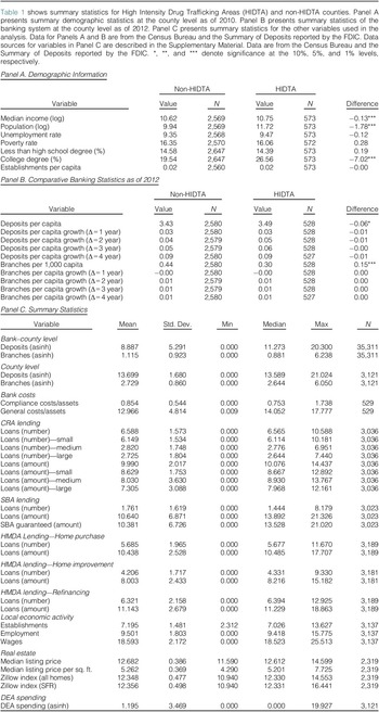
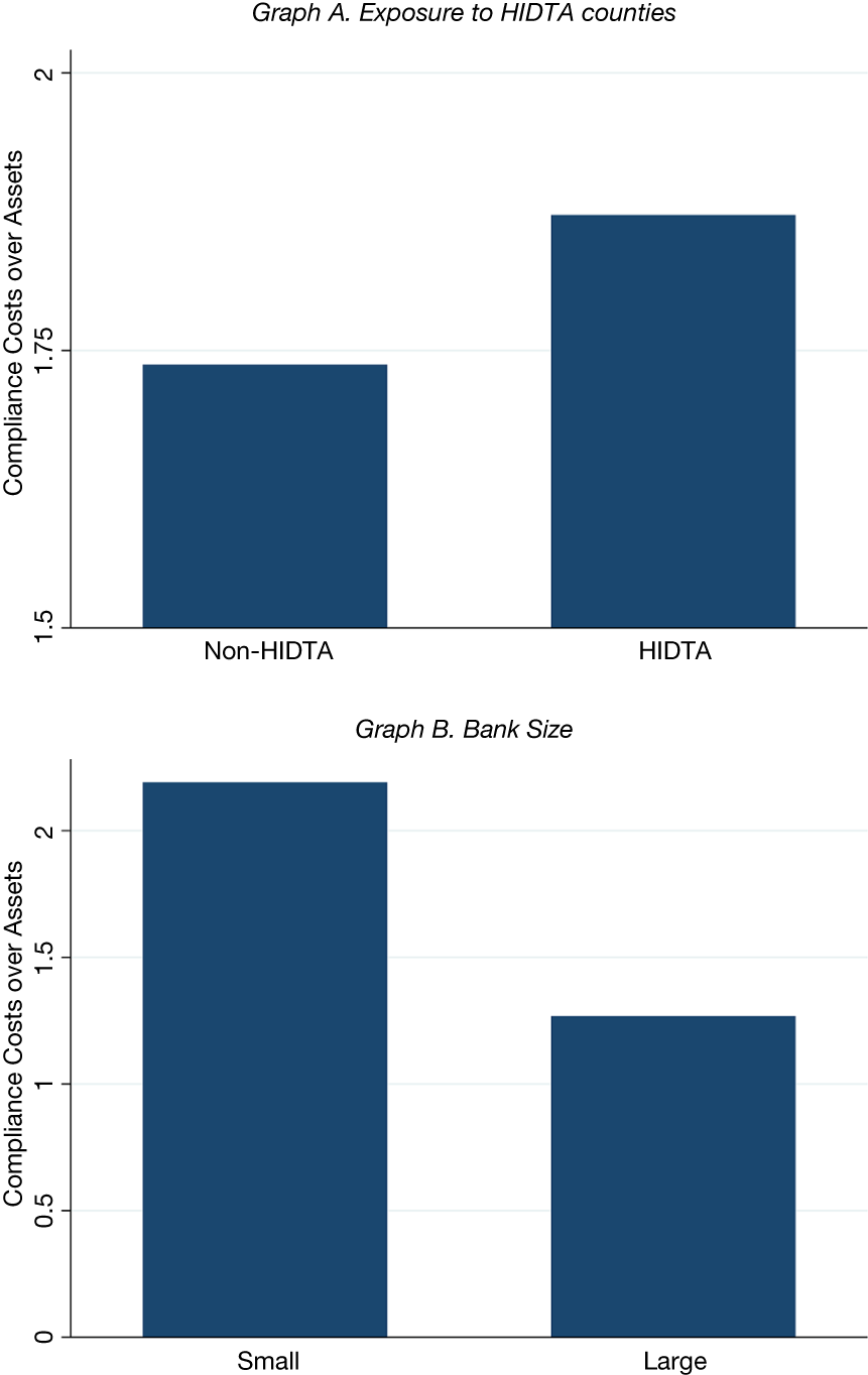


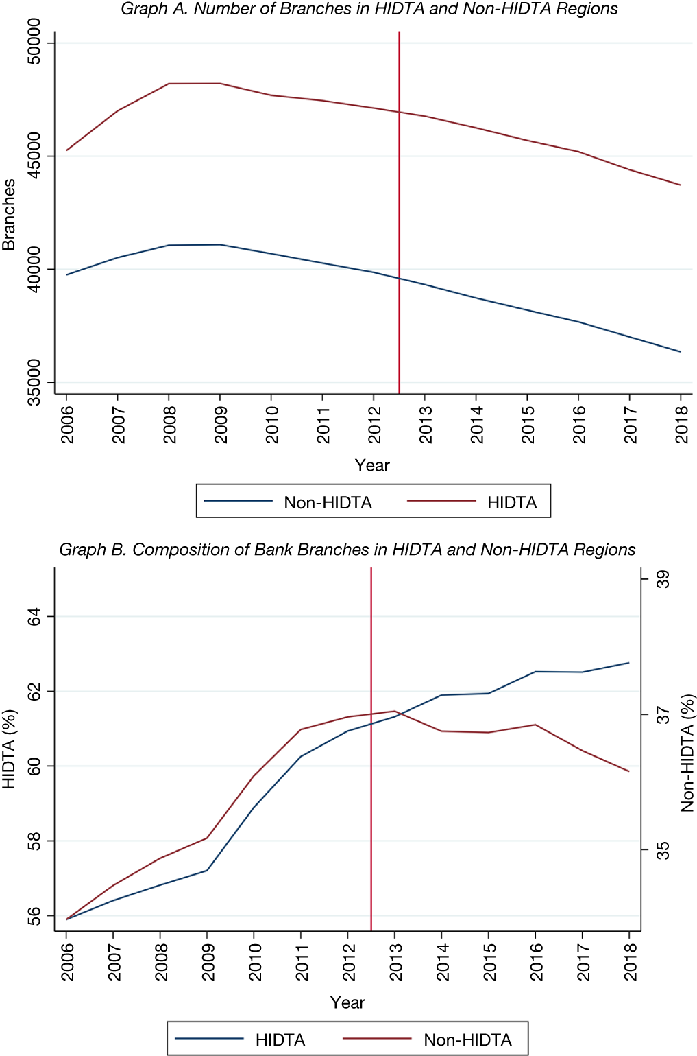

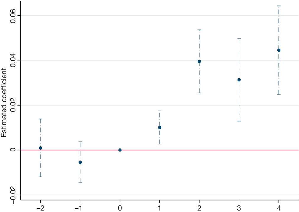


 Open access

