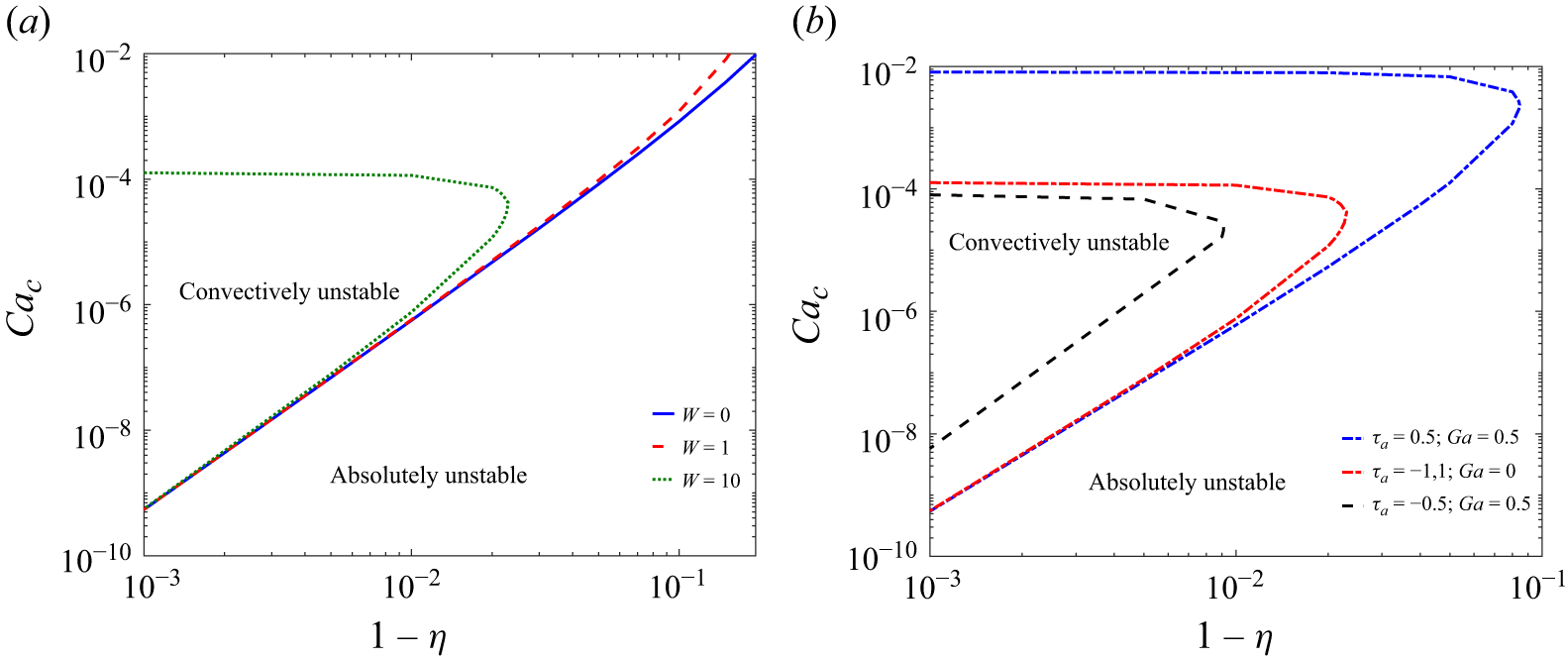
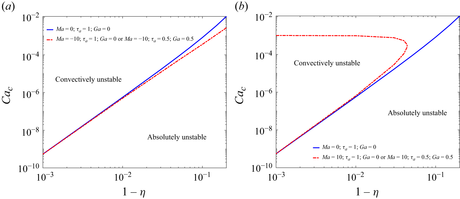
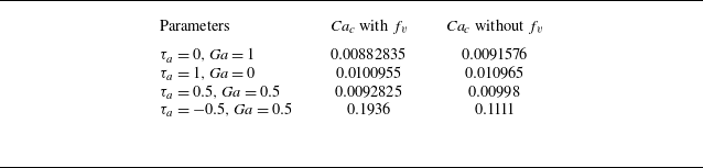
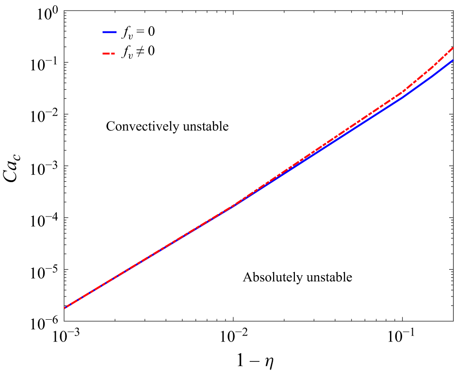
1. Introduction
The human lung consists of 23 airway generations, with the trachea being the zeroth airway generation and the terminal alveolar sacs being the last airway generation. Airways before the tenth generation, or inner diameter greater than
 $2$
mm, are generally termed proximal airways, and higher generation airways are termed distal airways. The proximal airways are characterised by turbulent airflow in contrast to the laminar airflow in the distal airways (Olson et al. Reference Olson, Sudlow, Horsfiel and Filley1973; Jain & Sznajder Reference Jain and Sznajder2007; Lin et al. Reference Lin, Tawhai, McLennan and Hoffman2007; Kleinstreuer & Zhang Reference Kleinstreuer and Zhang2009, Reference Kleinstreuer and Zhang2010; Xia et al. Reference Xia, Tawhai, Hoffman and Lin2010). Note that some analyses demand consideration of a laminar flow in the higher generations of proximal airways (
 $n\geqslant 2$
) during assisted ventilation, breathing at rest and under normal activity (Halpern, Jensen & Grotberg Reference Halpern, Jensen and Grotberg1998). The inner surface of the proximal airways is lined with airway surface liquid (ASL). It is made of two layers: the inner mucus layer and the outer serous layer. The ASL may lead to airway closure in the distal airways, even in healthy lungs, due to the film collapse triggered by the Rayleigh–Plateau instability (Heil, Hazel & Smith Reference Heil, Hazel and Smith2008; Romano et al. Reference Romano, Fujioka, Muradoglu and Grotberg2019; Erken et al. Reference Erken, Romano, Grotberg and Muradoglu2021, Reference Erken, Fazla, Muradoglu, Izbassarov, Romanò and Grotberg2023; Patne Reference Patne2025) in agreement with the clinical observations. Pulmonary diseases further enhance the possibility of airway closure in the distal airways (Mall Reference Mall2016; Patne Reference Patne2025). In contrast, recently, clinical observations have demonstrated the existence of ‘ASL plugs’ even in the proximal airways of patients with pulmonary diseases (e.g. asthma) (Huang, Elicker & Henry Reference Huang2024). Here, the ASL plug refers to the complete airway blockage by the thin ASL layer. Such plugs are absent in the healthy lungs.
Camassa, Ogrosky & Olander (Reference Camassa, Ogrosky and Olander2014) theoretically and experimentally analysed plug formation in a gravity-driven viscous film flow coating the interior of a tube. They demonstrated excellent agreement between the longwave theory-based model and the experimental observations. Their analysis predicted that absolute instability is a sufficient but not necessary condition for the formation of plugs in the tube. However, studies by Tseluiko & Kalliadasis (Reference Tseluiko and Kalliadasis2011), Ishimura et al. (Reference Ishimura, Mergui, Ruyer-Quil and Dietze2023), Dietze (Reference Dietze2024) predicted the formation of saturated-amplitude waves in an absolutely unstable film flow as an alternative path to the plug formation in certain parametric regimes. Thus, in contrast to the conclusions of Camassa et al. (Reference Camassa, Ogrosky and Olander2014), the occurrence of absolute instability is not a sufficient condition for plug formation. These contrasting predictions could only be resolved by solving the evolution equation derived in this work or performing experiments. In the present study, though, we focus on determining regions of absolute instability which could become guidelines for future numerical solutions or experiments. However, does the flow in the proximal airways even exhibit absolute instability? Can this explain the plugs in the proximal airways of diseased lungs? The present study aims to answer these questions and determine the relevant parametric regime for the existence of absolute instability in the proximal airways.
1.1. Thin film sheared by turbulent airflow
As discussed already, the turbulent airflow shears the ASL layer in the proximal airways (Lin et al. Reference Lin, Tawhai, McLennan and Hoffman2007). This shearing leads to the development of a linear velocity profile in the ASL layer. The stability of a Newtonian liquid layer of finite depth sheared by turbulent airflow was first analysed by Miles (Reference Miles1960). His analysis predicted a critical Reynolds number
 ${\textit{Re}}_c \sim 203$
at which the flow becomes temporally unstable in the limit of vanishing air–liquid interface tension. Here, the
 $Re$
is based on the maximum velocity, kinematic viscosity and thickness of the sheared liquid layer. Later, Smith & Davis (Reference Smith and Davis1982) predicted
 ${\textit{Re}}_c \sim 34$
for the same problem. This discrepancy between the predictions of Miles (Reference Miles1960) and Smith & Davis (Reference Smith and Davis1982) results from the missing term in the normal stress balance condition at the air–liquid interface used by Miles (Reference Miles1960).
In addition to the shearing by turbulent airflow, gravity also plays a role in driving the ASL flow. Camassa et al. (Reference Camassa, Forest, Lee, Ogrosky and Olander2012) mimicked this setting by considering a viscous liquid film lining the interior of the tube and driven against gravity by turbulent airflow up the core region of the tube. Their analysis demonstrated a qualitative agreement between the theoretical predictions using the long-wave theory-based model, namely the locally Poiseuille model and experimental observations. Camassa, Ogrosky & Olander (Reference Camassa, Ogrosky and Olander2017) extended the locally Poiseuille model of Camassa & Lee (Reference Camassa and Lee2006), Camassa et al. (Reference Camassa, Forest, Lee, Ogrosky and Olander2012, Reference Camassa, Ogrosky and Olander2014) by including first-order corrections to their locally Poiseuille model, signifying free-surface disturbances in the gas. This modified model exhibited a better quantitative agreement with the experimental observations of Camassa et al. (Reference Camassa, Forest, Lee, Ogrosky and Olander2012) compared with the locally Poiseuille model. Note that the locally Poiseuille model of Camassa et al. (Reference Camassa, Forest, Lee, Ogrosky and Olander2012) assumes slow air–ASL interface variations in the streamwise direction. This assumption allows the use of local information to estimate the turbulent stress exerted by the airflow and neglects the perturbations in the shear stresses.
Schmidt et al. (Reference Schmidt, Náraigh, Lucquiaud and Valluri2016) studied the occurrence of absolute instability in the countercurrent gas–liquid flow in a tube. Their results for the air–water-type system, relevant to the present study, showed that the linear stability theory succeeds in determining the most dominant features in the interfacial wave dynamics at early-to-intermediate times. Note that they assumed a laminar base state for both the phases in contradistinction with the turbulent airflow in the present analysis. Ishimura et al. (Reference Ishimura, Mergui, Ruyer-Quil and Dietze2023) studied the turbulent counter-current gas flow past a weakly inclined falling liquid film. They found a destabilising effect of the gas pressure, which amplifies the height of nonlinear Kapitza waves and exacerbates coalescence-induced formation of large-amplitude tsunami waves.
Tseluiko & Kalliadasis (Reference Tseluiko and Kalliadasis2011) studied a similar problem, albeit in an inclined channel using the weighted integral-boundary-layer (WRIBL) method. Their analysis predicted a destabilising effect of the turbulent airflow. Vellingiri, Tseluiko & Kalliadasis (Reference Vellingiri, Tseluiko and Kalliadasis2015) extended the analysis of Tseluiko & Kalliadasis (Reference Tseluiko and Kalliadasis2011) to determine the existence of absolute instability in a counter-current turbulent gas flow. At low and high airflow rates, they predicted a convectively unstable flow and an absolutely unstable flow for the intermediate range of airflow rates. Further, they concluded that the upper limit of the absolute instability region is close to the ‘flooding’ point characterised by large-amplitude standing waves predicted by Tseluiko & Kalliadasis (Reference Tseluiko and Kalliadasis2011). Thus, their analysis demonstrated that the onset of absolute instability can be used to predict the onset of flooding. Note that Tseluiko & Kalliadasis (Reference Tseluiko and Kalliadasis2011), Vellingiri et al. (Reference Vellingiri, Tseluiko and Kalliadasis2015) considered perturbations in the shear stress component of the airflow as well, in contrast with Miles (Reference Miles1960), Smith & Davis (Reference Smith and Davis1982), Camassa & Lee (Reference Camassa and Lee2006), Camassa et al. (Reference Camassa, Forest, Lee, Ogrosky and Olander2012) who considered only shear stress exerted by the turbulent airflow in the base state.
1.2. Flows in airways
Since our analysis is concerned with the flows in airways, next, we review studies dealing with flow stability in airways. Moriarty & Grotberg (Reference Moriarty and Grotberg1999) analysed the stability of airflow past a bilayer formed by a viscoelastic solid mucus layer and a Newtonian serous layer. Their analysis predicted a much lower airspeed necessary for the existence of the instabilities owing to the presence of the serous layer. Heil & White (Reference Heil and White2002) used nonlinear shell theory for the deformable airway wall to study airway closure due to airway wall-induced elastic instabilities for a Newtonian fluid lining the airway wall. Their analysis demonstrated that for large air–ASL interface tension, the airway wall can undergo a catastrophic collapse, which leads to a complete occlusion of airways. White & Heil (Reference White and Heil2005) derived a thin-film model to analyse airway closure due to the Rayleigh–Plateau instability and demonstrated that the non-axisymmetric instabilities allow the formation of occluding liquid bridges in situations in which the volume of fluid is insufficient to occlude the tube in its axisymmetric state. To analyse the effect of the ASL viscoelasticity on the instabilities in airways, Halpern, Fujioka & Grotberg (Reference Halpern, Fujioka and Grotberg2010) studied the stability of a viscoelastic film coating a rigid tube and flowing under the action of gravity, and predicted a destabilising influence of the viscoelasticity. However, they considered a static liquid layer coating the inside of a rigid cylindrical tube as the base state for their stability analysis. In our study, we consider a non-trivial base state.
To account for the impact of shear force exerted by the turbulent airflow and pulmonary surfactant on the ASL dynamics, Zhou et al. (Reference Zhou, Peng, Zhang and Zhuge2014) extended the study of Halpern et al. (Reference Halpern, Fujioka and Grotberg2010). For a range of parameters, in the absence of surfactant, their analysis predicted a stable base flow. Additionally, the surfactant was predicted to reinforce the viscoelastic effect of the film. Romano et al. (Reference Romano, Fujioka, Muradoglu and Grotberg2019) studied the liquid plug formation due to Rayleigh–Plateau instability and demonstrated the impact of airway closure on the airway epithelial layer. Romano et al. (Reference Romano, Muradoglu, Fujioka and Grotberg2021) analysed the impact of ASL viscoelasticity on airway closure and concluded the exacerbating effect of the ASL viscoelasticity in the airway closure. Erken et al. (Reference Erken, Romano, Grotberg and Muradoglu2021) showed the role of Rayleigh–Plateau instability in a two-layer liquid film lining the inner surface of a rigid tube as a model for liquid plug formation and closure of human airways. Considering the outcomes of analyses by Halpern et al. (Reference Halpern, Fujioka and Grotberg2010), Romano et al. (Reference Romano, Muradoglu, Fujioka and Grotberg2021), we will consider viscoelastic ASL.
Dietze & Ruyer-Quil (Reference Dietze and Ruyer-Quil2015) investigated the occlusion in narrow tubes due to nonlinear waves and demonstrated the role of nonlinear development of disturbances on airway closure using the weighted residual integral boundary layer (WRIBL) model to obtain the thin film equation. Similarly, Dietze, Lavalle & Ruyer-Quil (Reference Dietze, Lavalle and Ruyer-Quil2020) also used the WRIBL model and predicted occlusion in a narrow cylindrical tube due to gravity-driven liquid film falling down the inner surface in the presence of an active core gas flow. An analytical treatment of two-layer thin film flows and the application of the longwave model along with the WRIBL model to such flows is discussed at length by Dietze (Reference Dietze2022). The analyses by Dietze & Ruyer-Quil (Reference Dietze and Ruyer-Quil2015) and Dietze et al. (Reference Dietze, Lavalle and Ruyer-Quil2020) focused on the occlusion of a narrow tube due to the development of instabilities into spatially growing waves and reported the parametric regime in which tube occlusion could occur.
Dietze (Reference Dietze2024) analysed core-annular flow of air (core fluid) and a Newtonian liquid (annular fluid) to study liquid plugs in the pulmonary airways by employing a two-phase axisymmetric WRIBL model of Dietze et al. (Reference Dietze, Lavalle and Ruyer-Quil2020). His analysis established a continuous path from travelling-wave solutions to travelling-plug solutions and predicted the critical airway generation for liquid-plug formation for a given value of the liquid hold up. The 16th airway generation requires the least liquid hold up volume for the liquid plug formation. As airway generation increases, the critical liquid hold up volume necessary for liquid plug formation also increases. His analysis demonstrated that the liquid volume hold up necessary for 6th or lower generations is quite unlikely to be encountered in a physiological setting. Salin & Talon (Reference Salin and Talon2019) analysed the transition from convective to absolute instability in a core-annular flow of two immiscible Newtonian fluids. Their analysis considered both viscosity and density stratification and investigated the effect of various parameters on the transition.
Additionally, there have been several studies dealing with the flows of a viscoelastic fluid down an inclined plane, which could be relevant to the ASL flows in airways. Gupta (Reference Gupta1967) revealed the existence of growing shear waves due to fluid elasticity. Gupta & Rai (Reference Gupta and Rai1967) predicted a destabilising effect of the viscoelastic nature of the fluid. The analysis by Shaqfeh, Larson & Fredrickson (Reference Shaqfeh, Larson and Fredrickson1989) using the Oldroyd-B model predicted that the fluid viscoelasticity has a small destabilising effect on the film stability for small Reynolds numbers. Meanwhile, fluid viscoelasticity stabilises the film for moderate Reynolds numbers. Thus, the fluid elasticity could be of little importance in practical situations. Kang & Chen (Reference Kang and Chen1995) predicted the existence of a purely elastic instability for a very thin film using the longwave evolution equation. Uma & Usha (Reference Uma and Usha2004) investigated the effect of interfacial phase change on the stability of the film. They predicted the possibility of both supercritical stability and subcritical instability for condensate, evaporating and isothermal viscoelastic film flow systems depending on the parameters. Zhou et al. (Reference Zhou, Peng, Zhang and Zhuge2016), by employing Shkadov’s integral boundary layer method, analysed the stability of an annular viscoelastic film flowing down a flexible tube. Their results further demonstrated the destabilising role of the fluid viscoelasticity, while the tube flexibility, which includes wall damping and wall tension, was found to play a dual role. Hu et al. (Reference Hu, Fu, Xing, Yang and Xie2021) used the WRIBL model to derive a thin film evolution equation in the weak viscoelastic limit. Their predictions affirmed the destabilising role of fluid viscoelasticity and the existence of a purely elastic instability in gravity-driven flow.
Patne (Reference Patne2022) considered a thin shear-thinning viscoelastic film lining a deformable solid layer and sheared by turbulent airflow as a model for ASL lining airways. His analysis predicted the existence of purely elastic instabilities due to the elasticity of the ASL and airway wall. Romano, Muradoglu & Grotberg (Reference Romano, Muradoglu and Grotberg2022) predicted delays in the ASL plug formation and lower stresses on the airway wall during ASL plugging due to the presence of pulmonary surfactant. Erken et al. (Reference Erken, Fazla, Muradoglu, Izbassarov, Romanò and Grotberg2023) investigated the effect of the elastoviscoplastic properties of the ASL on airway closure and predicted lethal or sublethal damage to the airway epithelial cells exacerbated by ASL elasticity. Shemilt et al. (Reference Shemilt, Horsley, Jensen, Thompson and Whitfield2022) derived an evolution equation for an axisymmetric layer of a Bingham liquid coating the interior of a tube as a model for an airway lined with viscoplastic mucus. The numerical solution of the derived evolution equation predicted an increase in the critical layer thickness required to form a liquid plug in the tube due to ASL yield stress. Shemilt et al. (Reference Shemilt, Horsley, Jensen, Thompson and Whitfield2023) predicted the inhibition of the capillary instability and delay in airway closure due to the surfactant. Patne (Reference Patne2024) analysed the effect of inhaled air temperature on mucus dynamics in the proximal airways. He predicted a strong stabilising/destabilising effect if the inhaled air is warmer/colder than body temperature. Camassa, Ogrosky & Olander (Reference Camassa, Ogrosky and Olander2024) analysed the dynamics of a gravity-driven upper convected Maxwell fluid film coating the inner surface of a tube. Their analysis predicted the enhancement of the instability growth rate and the promotion of absolute instability due to fluid elasticity. Recently, Patne (Reference Patne2025) demonstrated the possibility of absolute instability-induced airway closure in the distal airways, where a core-annular flow of air and ASL can exist, in agreement with the clinical observations.
In the proximal airways, the motion of airway surface liquid (ASL), which coats the interior surface of airways, is governed by gravity and turbulent airflow. Thus, the predictions of the previous analyses by Camassa et al. (Reference Camassa, Forest, Lee, Ogrosky and Olander2012, Reference Camassa, Ogrosky and Olander2014), Camassa & Ogrosky (Reference Camassa and Ogrosky2015), Vellingiri et al. (Reference Vellingiri, Tseluiko and Kalliadasis2015), Camassa et al. (Reference Camassa, Ogrosky and Olander2024) become relevant for the proximal airways. In their analysis, Camassa et al. (Reference Camassa, Forest, Lee, Ogrosky and Olander2012, Reference Camassa, Ogrosky and Olander2014) considered a Newtonian fluid lining the tube, neglected the shearing by the airflow and assumed an isothermal airflow. Camassa & Ogrosky (Reference Camassa and Ogrosky2015), Camassa et al. (Reference Camassa, Ogrosky and Olander2017) did consider the role of turbulent airflow shearing a Newtonian film along with gravity; however, they analysed only temporal stability analysis. Camassa et al. (Reference Camassa, Ogrosky and Olander2024) considered only the gravity-driven flow of a viscoelastic fluid. The ASL is a strongly viscoelastic fluid owing to the presence of mucins, the shearing action by the turbulent airflow will act as a driving force and from previous analysis of Patne (Reference Patne2024), inhaled air temperature can have a strong impact on the ASL dynamics. Thus, the ASL dynamics could be drastically different from the dynamics predicted by Camassa et al. (Reference Camassa, Forest, Lee, Ogrosky and Olander2012, Reference Camassa, Ogrosky and Olander2014), Camassa & Ogrosky (Reference Camassa and Ogrosky2015), Camassa et al. (Reference Camassa, Ogrosky and Olander2017, Reference Camassa, Ogrosky and Olander2024).
Vellingiri et al. (Reference Vellingiri, Tseluiko and Kalliadasis2015) considered the countercurrent gas–Newtonian liquid flow in the presence of gravity, but for flow in an inclined plane. However, the flow geometry relevant to the ASL flow in airways should be cylindrical since azimuthal curvature in cylindrical geometry will lead to capillary instability. As demonstrated by Camassa et al. (Reference Camassa, Ogrosky and Olander2014, Reference Camassa, Ogrosky and Olander2024) and discussed later in § 5, this will play a major role in determining the existence of absolute instability.
Owing to the shortcomings of Camassa et al. (Reference Camassa, Forest, Lee, Ogrosky and Olander2012, Reference Camassa, Ogrosky and Olander2014), Camassa & Ogrosky (Reference Camassa and Ogrosky2015), Camassa et al. (Reference Camassa, Ogrosky and Olander2017, Reference Camassa, Ogrosky and Olander2024), Vellingiri et al. (Reference Vellingiri, Tseluiko and Kalliadasis2015), in the present study, we investigate the absolute instability in cylindrical flow geometry by considering the viscoelastic fluid sheared by turbulent airflow with inhaled air temperature differing from body temperature. Additionally, we employ the locally Poiseuille model of Camassa & Lee (Reference Camassa and Lee2006), Camassa et al. (Reference Camassa, Forest, Lee, Ogrosky and Olander2012, Reference Camassa, Ogrosky and Olander2014). As noted by Camassa et al. (Reference Camassa, Ogrosky and Olander2017), their model predicts a higher temporal growth rate for instability compared with the locally Poiseuille model. Thus, the Camassa et al. (Reference Camassa, Ogrosky and Olander2017) model could predict a larger absolute instability region than the locally Poiseuille model employed here. This leads to the conclusion that if the model used here predicts absolute instability for a set of parameters, then the Camassa et al. (Reference Camassa, Ogrosky and Olander2017) model will also predict the presence of absolute instability for the same set of parameters. As discussed later in § 5, even with the locally Poiseuille model, the predictions of our analysis are in good agreement with the clinical observations of Huang et al. (Reference Huang2024), thereby justifying the considered model. The flow in the airways is time-periodic in nature due to the breathing cycle. To carry out stability analysis of this flow would require spatio-temporal stability analysis of time-periodic flow. To the best of the authors’ knowledge, such a procedure is not available in the literature. Thus, in the present study, we consider time-independent flow over a range of velocities to account for velocity variation during the breathing cycle.
The rest of the paper is arranged as follows. The governing equations, boundary conditions and base state are presented in § 2. The longwave evolution equation is derived in § 3. The dispersion relation derivation and temporal stability analysis are presented in § 4. The parametric regions of absolutely and convectively unstable flow are presented in § 5. Finally, the major conclusions obtained in the present study are presented in § 6.
2. Problem formulation
We consider an incompressible viscoelastic liquid layer film of constant dynamic viscosity
 $\mu ^*$
, density
 $\rho ^*$
and relaxation time
 $\lambda ^*$
lining the inner side of a rigid tube of inner radius
 $r_o^*$
. The superscript ‘
 $*$
’ signifies a dimensional quantity. The ASL layer is present in the annular gap
 $r \in [r_i^*,r_o^*]$
possessing thickness
 $R^* =r_o^* - r_i^*$
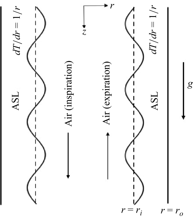
. The ASL is flowing under the combined action of the gravity and shear stress exerted by the core turbulent airflow. The schematic of the flow model considered in this work is shown in figure 1. The turbulent airflow exerts shear stress
 $\tau ^*_a = 1/2 \, c^*_f \, \rho ^*_a \, V_a^{*2}$
with
 $c^*_f =0.02$
, where
 $\rho ^*_a$
and
 $V_a^{*}$
are the density and velocity of the air, respectively (Pedley Reference Pedley1977; Miesen & Boersma Reference Miesen and Boersma1995). The formula for
 $\tau ^*_a$
is applicable provided that a fully developed core turbulent airflow exists and ASL thickness is much smaller than the airway radius. During inspiration, the turbulent airflow will be in the direction of gravity, thus,
 $\tau ^*_a \gt 0$
and the opposite during expiration. Note that we have assumed
 $V_a^{*}$
to be constant to make the problem tractable.
Schematic of the flow geometry considered in the present system in dimensionless coordinates. The airflow direction is in the direction of gravity during inspiration and opposite during expiration. The airflow shears the ASL and leads to thermal energy exchange. Due to air temperature being different from body temperature, a radial temperature gradient occurs across the ASL layer, indicated by the equation
 $ {{\rm d} T}/{{\rm d} r}= {1}/{r}$
in the ASL layer in dimensionless terms.

Starting from the fourth airway generation, the orientation of airflow during inspiration can indeed be either opposed to or aligned with gravity within the same airway generation (Weibel Reference Weibel1963). An opposite scenario exists for expiration. This arises because of the following.
-
(i) Airway branching geometry becomes complex and three-dimensional from around generation 4 onwards (starting roughly from the segmental bronchi and beyond).
-
(ii) The trachea (generation 0) and early bronchi (generations 1–3) are mostly oriented near-vertically in upright posture, meaning airflow during inspiration is largely aligned with gravity (air moves downwards).
-
(iii) However, from generation 4 onwards (subsegmental bronchi and smaller bronchi), airway branches extend into different lobes and segments of the lung, having orientations both upward and downward relative to gravity.
Due to this, in the upper lobes, bronchi may branch upwards or horizontally relative to gravity in the upright position, so airflow during inspiration is opposed to gravity there. In the lower lobes, bronchi continue branching downwards, so airflow remains aligned with gravity. Thus, for the proximal airways in the upper lobes of the lungs, airflow directions will be opposite to that shown in figure 1.
The inhaled air is assumed to be at a temperature different from the body temperature to account for the air temperature effect on the ASL dynamics. The human muscles exhibit poor heat conduction (El-Brawany et al. Reference El-Brawany, Nassiri, Terhaar, Shaw, Rivens and Lozhken2009); thus, at
 $r^*=r_o^*$
, we assume a poorly conducting substrate. Following previous analyses of Pearson (Reference Pearson1958), Oron, Davis & Bankoff (Reference Oron, Davis and Bankoff1997), Patne (Reference Patne2024), we consider that the ASL is subjected to a radial temperature gradient
 $\beta ^*= ({r^*}/{R^*})( {\partial T^*}/{\partial r^*})$
. Note that poor conductivity of airway epithelial cells could lessen
 $\beta ^\star$
.
To non-dimensionalise the governing equations, the lengths, time and temperature are scaled by
 $R^*$
,
 $R^{*2}/V^*_s$
and
 $\beta ^* R^*$
, respectively, where
 $V_s^*=\rho ^* g^* R^{*2}/\mu ^*+R^* |\tau ^*_a|/\mu ^*$
. This choice of velocity scale allows extreme cases with purely turbulent air-driven flow, purely gravity-driven flow, and combined gravity and turbulent air-driven flow. The pressure and stresses are non-dimensionalised by
 $\mu ^* V^*_s/R^*$
. Let
 $\boldsymbol{v}=(v_r,v_z)$
,
 $p$
,
 $\boldsymbol{\tau }$
and
 $T$
be the dimensionless velocity, pressure, stress and temperature fields in the ASL, respectively. This procedure yields the dimensionless continuity, Cauchy momentum and energy equations,
 \begin{align} \boldsymbol{\nabla }\boldsymbol{\cdot }\boldsymbol{v}&=0, \end{align}
 \begin{align} \textit{Re} \, \left [\frac {\partial \boldsymbol{v}}{\partial t}+(\boldsymbol{v}\boldsymbol{\cdot }\boldsymbol{\nabla }) \, \boldsymbol{v} \right ]&= -\boldsymbol{\nabla }p + \boldsymbol{\nabla }\boldsymbol{\cdot }\boldsymbol{\tau } + Ga \, \hat {e}_z, \end{align}
 \begin{align} \textit{Re} \, \textit{Pr} \, \left [\frac {\partial T}{\partial t}+(\boldsymbol{v}\boldsymbol{\cdot }\boldsymbol{\nabla }) \, T \right ]&={\nabla} ^2 T, \end{align}
where
 $Re=\rho ^* V^*_s R^*/\mu ^*$
,
 ${\textit{Ga}} = \rho ^* g^* R^{*2}/(\mu ^* V^*_s)$
,
 $Pr = \mu ^*/(\rho ^* \alpha ^*)$
are the Reynolds, Galileo (or Galilei) and Prandtl numbers, respectively, and
 $\boldsymbol{\nabla}$
is the gradient operator. Note that the Galileo number is a ratio of the Bond number
 $Bo=\rho ^* g^* R^{*2}/(\varSigma ^*_0)$
and the capillary number
 ${\textit{Ca}} = \mu ^* V^*_s/\varSigma ^*_0$
. Also, in terms of scaled variables,
 $r_i=\eta /(1-\eta )$
and
 $r_o=1/(1-\eta )$
, where
 $\eta =r_i^*/r_o^*$
.
Owing to the viscoelastic nature of the ASL, here, we employ the upper convective Maxwell (UCM) model (Halpern et al. Reference Halpern, Fujioka and Grotberg2010; Camassa et al. Reference Camassa, Ogrosky and Olander2024; Patne Reference Patne2024)
 \begin{eqnarray} \boldsymbol{\tau }+W \left [ \frac {\partial \boldsymbol{\tau }}{\partial t} + \boldsymbol{v} \boldsymbol{\cdot }\boldsymbol{\tau }- (\boldsymbol{\nabla }\boldsymbol{v})^T \boldsymbol{\cdot }\boldsymbol{\tau }-\boldsymbol{\tau } \boldsymbol{\cdot }(\boldsymbol{\nabla }\boldsymbol{v}) \right ]= \boldsymbol{\dot \gamma }, \end{eqnarray}
where
 $W=\lambda ^* V^*_s/ R^*$
is the Weissenberg number and
 $\boldsymbol{\dot \gamma }=(\boldsymbol{\nabla }\boldsymbol{v})+(\boldsymbol{\nabla }\boldsymbol{v})^T$
is the strain-rate tensor. Note that we have neglected the solvent contribution to the stress field in the ASL for mathematical convenience. This can be justified due to the large viscosity difference between the ASL and solvent (water), leading to a negligible solvent contribution.
Due to the difference in the temperature of the inhaled air (
 $T_a^*$
) and airway muscle temperature (
 $T_m^*$
), a temperature gradient could exist across the air–ASL interface. This will give rise to thermocapillary stresses owing to thermocapillarity. Here, we assume linear dependence of the surface tension (
 $\varSigma ^*$
) on the temperature of the interface (
 $T^*$
) (Pearson Reference Pearson1958; Oron et al. Reference Oron, Davis and Bankoff1997). Thus,
 $\varSigma ^* = \varSigma _0^* - \gamma ^* (T^*-T_0^*)$
, where
 $\varSigma _0^*$
is the air–liquid interface tension at the reference temperature
 $T_0^*$
and
 $\gamma ^* = -( {{\rm d} \varSigma ^*}/{{\rm d} T^*})$
.
The above-mentioned equations are subjected to the following boundary conditions. At the dimensionless air–ASL interface (
 $r=r_i$
), we impose the kinematic boundary condition, stress balance conditions and continuity of heat flux,
 \begin{align} \frac {\partial h}{\partial t} + v_z \frac {\partial h}{\partial z}&=v_r, \end{align}
 \begin{align} \boldsymbol{t} \boldsymbol{\cdot }\boldsymbol{\tau } \boldsymbol{\cdot }\boldsymbol{n} + \tau _a &= -\textit{Ma} \, \boldsymbol{\nabla }T \boldsymbol{\cdot }\boldsymbol{t}, \end{align}
 \begin{align} -p+ \boldsymbol{n} \boldsymbol{\cdot }\boldsymbol{\tau } \boldsymbol{\cdot }\boldsymbol{n} &= \frac {1}{\textit{Ca}} \boldsymbol{\nabla }\boldsymbol{\cdot }\boldsymbol{n}, \end{align}
 \begin{align} \boldsymbol{\nabla }T \boldsymbol{\cdot }\boldsymbol{n} + \textit{Bi} (T-T_a)&=0, \end{align}
where
 $\boldsymbol{t}$
and
 $\boldsymbol{n}$
are the unit tangent and normal to the air–ASL interface, respectively. The parameters
 $\tau _a= R^* \tau ^*_a/(\mu ^* V_s^*)$
,
 $Ma=\gamma ^* \beta ^* R^*/(\mu ^* V^*_s)$
and
 $Bi=q^* R^*/k^*_t$
are the dimensionless shear stress exerted by the turbulent airflow and Marangoni and Biot numbers, respectively, with
 $q^*$
as the coefficient of heat convection or heat transfer coefficient at the air–ASL interface.
As noted in § 1, here, we use a locally Poiseuille-flow model. Next, we provide an estimate of the error committed in assuming a locally Poiseuille-flow model compared with a non-local model of Tseluiko & Kalliadasis (Reference Tseluiko and Kalliadasis2011). From the analysis of Tseluiko & Kalliadasis (Reference Tseluiko and Kalliadasis2011), consideration of the non-local interfacial stresses implies
 $\tau _a = \tau _{a0} + \epsilon \tau _{a1} e^{i k z}$
(see their (3.41)). The model used in our study considers only
 $\tau _{a0}$
, while ignoring the term
 $\epsilon \tau _{a1} e^{i k z}$
. Thus, the error committed by our model is proportional to the same term. Since
 $\epsilon$
is an arbitrarily small perturbation parameter and
 $e^{i k z}$
is a purely oscillatory term for temporal stability analysis, the value of the correction due to consideration of the locally Poiseuille-flow model is proportional to
 $\tau _{a1}$
. From figure 5 of Tseluiko & Kalliadasis (Reference Tseluiko and Kalliadasis2011), as the wavenumber of perturbations, i.e.
 $k \rightarrow 0$
,
 $\tau _{a1}\sim 0.01$
and highest for
 $k=0.1$
with
 $\tau _{a1} \sim 0.51$
. Thus, longwave perturbations are least affected by the locally Poiseuille-flow model assumptions. The error introduced by the assumption of a locally Poiseuille-flow model in stress calculation is of
 $O(10^{-3}-10^{-2})$
, if we assume
 $\epsilon =0.1$
.
At
 $r=r_o$
, we impose no-slip, impermeability and zero heat flux boundary conditions,
 \begin{eqnarray} v_z=0, \quad v_r=0, \quad { \frac {\partial T}{\partial r}=0.} \end{eqnarray}
2.1. Base state
As discussed later, to incorporate the effect of ASL elasticity, the knowledge of base-state velocity is necessary. Similarly, to understand the impact of thermocapillarity, the base state temperature gradient is necessary. Thus, we derive the base state as follows. For a steady, axisymmetric, fully developed base state, the quantities are
 \begin{align}& \bar v_z = \frac {\textit{Ga}}{4} (r_o^2- r^2) + \left ( \frac { r_i^2 \, \textit{Ga}}{2} - r_i \, \tau _a \right ) \log (r/r_o), \end{align}
 \begin{align}&\qquad\qquad \bar \tau _{rz}=\frac {{\rm d} \bar v_z}{{\rm d}r}; \quad \bar \tau _{zz}=2W \bar \tau _{rz} \frac {{\rm d} \bar v_z}{{\rm d}r}, \end{align}
 \begin{align}&\qquad\qquad\qquad\qquad \frac {{\rm d} \bar T}{{\rm d}r} = \frac {1}{r}. \end{align}
By the definition of
 $\tau _a$
,
 $\tau _a$
is positive during inspiration and
 $\tau _a$
is negative during expiration due to change in the sign of
 $\tau ^*_a$
. Thus, during inspiration, the turbulent airflow will reinforce the gravity-driven ASL flow, while during expiration, an opposite scenario will occur.
Next, the range of relevant parameters is estimated as follows. The radius of the proximal airways (
 $r_o^*$
) is of
 $\sim O(10^{-3})$
m, and for a healthy lung, the thickness of the ASL is
 $\sim O(10^{-6}-10^{-5})$
m (Widdicombe & Widdicombe Reference Widdicombe and Widdicombe1995; Widdicombe Reference Widdicombe1997; Moriarty & Grotberg Reference Moriarty and Grotberg1999; Furlow & Mathisen Reference Furlow and Mathisen2018; Karamaoun et al. Reference Karamaoun, Sobac, Mauroy, Van Muylem and Haut2018). From this,
 $r_i^*$
can be estimated by subtracting ASL thickness from the radius of airways. This shows that, for a healthy lung,
 $r_i^* \sim r_o^*$
owing to the very small thickness of the ASL; thus,
 $\eta = r_i^*/r_o^* \sim 1$
. However, due to respiratory diseases, the thickness of the mucus layer could substantially increase; thus,
 $\eta$
could substantially differ from unity (Shah et al. Reference Shah, Scott, Knight, Marriott, Ranasinha and Hodson1996; Moriarty & Grotberg Reference Moriarty and Grotberg1999).
The density, relaxation time, air–mucus interface tension and viscosity of the mucus are
 ${\sim} 10^{3}$
kg m−
 $^3$
,
 ${\sim} 10^{-3}{-}1$
s,
 ${\sim} 10^{-1}{-}10^{-2}$
N m−1 and
 ${\sim} 10^{-2}{-}10^{2}$
Pa s, respectively, and
 $\gamma ^* \sim 10^{-5}{-}10^{-3}$
N (m K)−1 (Hwang, Litt & Forsman Reference Hwang, Litt and Forsman1969; Lai et al. Reference Lai, Wang, Wirtz and Hanes2009; Hamed & Fiegel Reference Hamed and Fiegel2014; Hill et al. Reference Hill2014; Chen et al. Reference Chen, Zhong, Luo, Deng, Hu and Song2019). The average velocity of the airflow in the proximal airways is
 $V^*_a \sim 10{-}0.4$
m s−1 (Pedley Reference Pedley1977). Note that from the table provided by Pedley (Reference Pedley1977), as the air travels to the higher generation of airways beyond the trachea, the airflow speed first increases up to the third generation and then decreases for the later generations. Due to turbulent airflow, we use the formula
 $\tau ^*_a = 1/2 \, c^*_f \, \rho ^*_a \, V_a^{*2}$
with
 $c^*_f =0.02$
to obtain
 $V^*_s \sim 10^{-3}{-}10^{-6}$
m s−1 (Miesen & Boersma Reference Miesen and Boersma1995). Note that
 $c^*_f$
will increase with increasing generation number and
 $c^*_f =0.008{-}0.023$
for proximal airways. Note that the
 $c_{f}^{*}$
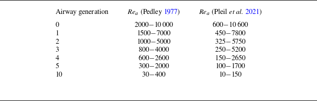
value considered here could be lower than the actual value for 7–10 airway generations since the turbulence intensity is low for these generations. The Reynolds number for different proximal airway generations is given in table 1, as given by Pedley (Reference Pedley1977). The peak inspiration and expiration volumetric airflow rates, as mentioned in the literature by Pedley, Schroter & Sudlow (Reference Pedley, Schroter and Sudlow1970), Pedley (Reference Pedley1977), Mead (Reference Mead1978), Weibel (Reference Weibel1984), West (Reference West2012), are
 $q=0.4{-}0.6$
l s−1 during quiet or normal breathing and
 $q=0.9{-}2.4$
l s−1 for vigorous breathing. Note that the phrase ‘peak volumetric flow rate’ implies the highest airflow rate during the expiration and inspiration phases of the breathing cycle. Considering
 $d=1.8$
cm trachea diameter, the airflow Reynolds number
 ${\textit{Re}}_a=2q/(\pi {\rm d} \nu )$
is in the range of
 $2000{-}10\,000$
, where
 $\nu$
is the kinematic viscosity of air. This estimated range is in agreement with the data reported in table 1 of Pedley (Reference Pedley1977). Similar calculations provide a range of
 ${\textit{Re}}_a$
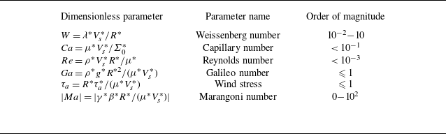
shown in table 1. The order of magnitude of the dimensionless parameters is given in table 2.
Airway generations and corresponding airflow Reynolds number (
 ${\textit{Re}}_a$
) from Pedley (Reference Pedley1977), Pleil, Stiegel & Risby (Reference Pleil, Stiegel and Risby2021). The difference between the Reynolds number values from Pedley (Reference Pedley1977) and Pleil et al. (Reference Pleil, Stiegel and Risby2021) could be due to the average volumetric flow rate considered by the latter, while the former considers peak volumetric flow rates.

Order of magnitude of the dimensionless parameters using the dimensional parameters. Due to pulmonary diseases, higher values of
 $W$
are accessible due to increased ASL viscosity and elasticity.

3. Longwave evolution equation
From previous analyses of Patne (Reference Patne2022, Reference Patne2024), the ASL layer exhibits longwave instabilities. Additionally, Camassa et al. (Reference Camassa, Ogrosky and Olander2014) demonstrated excellent agreement between experimental observations and theoretical predictions obtained from the longwave evolution equation for a setting similar to that considered in this work. Thus, in this section, we derive a longwave evolution equation describing the dynamics of the liquid layers for the disturbances. If
 $\varLambda$
is the wavelength of the perturbations, then we define a parameter
 $\epsilon \ll 1$
such that
 $R=\epsilon \varLambda$
. Now, following the procedure described by Oron et al. (Reference Oron, Davis and Bankoff1997), Samanta (Reference Samanta2013), Patne, Agnon & Oron (Reference Patne, Agnon and Oron2021), Patne & Chandarana (Reference Patne and Chandarana2023), Patne (Reference Patne2025), we scale the
 $z$
-axis and time as
 $z \to Z \epsilon ^{-1}$
and
 $t \to \tau \epsilon ^{-1}$
. The fluid dynamical quantities are expanded as
 \begin{align} v_z &= u_0+ \epsilon ^2 u_2+\ldots , \end{align}
 \begin{align} v_r &= \epsilon \bigl( v_0+ \epsilon ^2 v_2+\ldots \bigr), \end{align}
 \begin{align} p &= \frac {1}{\epsilon } \bigl(\varPi _0+ \epsilon ^2 \varPi _2+\ldots \bigr). \end{align}
As noted by Patne (Reference Patne2022, Reference Patne2024), the elastic mode arises due to the first normal stress difference across the air–ASL interface. The other elastic terms in the constitutive equations involving
 $W$
provide a negligible quantitative correction in the absence of the gravity effect. This aspect has been discussed in detail by Patne (Reference Patne2025) for core-annular flow. Due to this, we neglect elastic terms in the constitutive (2.1d
), while retaining the relevant term in the tangential stress balance condition at the air–ASL interface. As a consequence of this assumption, the ASL elasticity will affect the stability only through the air–ASL interface tangential stress balance condition. In the constitutive (2.1d
), if we retain the elastic terms, i.e. the term containing
 $W$
, then the resulting expanded equations upon substitution of longwave scaling cannot be solved by analytical methods since this leads to the equations for stress components and their derivatives. We must solve the scaled constitutive equations even for stress components, which becomes a mathematically intractable problem. The other possibility that can successfully capture the elastic effects, yet the problem is analytically solvable, is by considering the most crucial elastic term in the tangential stress balance condition at the air–ASL interface. This term leads to the elastic instability in the turbulent air-driven ASL flow problem. In the subsequent derivation, we first obtain the
 $O(1)$
equation, which does not include the effect of axial viscous diffusion and later add the effect of axial viscous diffusion entering at
 $O(\epsilon ^2)$
.
3.1. No axial viscous diffusion
The inertial terms are negligibly small for the ASL layer due to
 $Re \ll 1$
, which allows us to neglect those terms. Upon substitution of the expansions (3.1), the governing continuity and momentum equations become
 \begin{align} \frac {1}{r} \partial _r \left [ r \bigl(v_0+\epsilon ^2 v_2\bigr) \right ]+ \partial _Z \bigl(u_0+\epsilon ^2 u_2\bigr)&=0, \end{align}
 \begin{align} \epsilon ^2 \left [ \frac {1}{r} \partial _r \left ( r \partial _r \right ) + \epsilon ^2 \partial ^2_Z - \frac {1}{r^2} \right ] \bigl(v_0+\epsilon ^2 v_2\bigr) - \partial _r \bigl(\varPi _0+\epsilon ^2 \varPi _2\bigr)&=0, \end{align}
 \begin{align} \left [ \frac {1}{r} \partial _r \left ( r \partial _r \right ) + \epsilon ^2 \partial ^2_Z \right ] \bigl(u_0+\epsilon ^2 u_2\bigr) - \partial _Z \bigl(\varPi _0+\epsilon ^2 \varPi _2\bigr) + \textit{Ga} &=0. \end{align}
For the temperature, following Oron et al. (Reference Oron, Davis and Bankoff1997), Patne et al. (Reference Patne, Agnon and Oron2021), the imposed temperature gradient effect will directly enter through the tangential boundary condition at the air–ASL interface as discussed in the following.
Upon substitution of the expansions (3.1) in the boundary conditions (2.2) except for the kinematic boundary condition, we obtain
 \begin{align} &2 \epsilon ^2 [ \partial _r (v_0+\epsilon ^2 v_2)-\partial _Z (u_0+\epsilon ^2 u_2)] \partial _Z \zeta + [1 - \epsilon ^2 (\partial _Z \zeta )^2] \partial _r (u_0+\epsilon ^2 u_2) \nonumber \\&\quad + [1 - \epsilon ^2 (\partial _Z \zeta )^2] \epsilon ^2 \partial _Z (v_0+\epsilon ^2 v_2) + \left (\frac {\widehat {\textit{Ma}}}{\zeta } -2\widehat {W}_m \right ) \partial _Z \zeta + \tau _a = 0, \end{align}
 \begin{align}& -(\varPi _0+\epsilon ^2 \varPi _2)[1 + (\partial _Z \zeta )^2] + 2 \epsilon ^2 \partial _r (v_0+\epsilon ^2 v_2) + 2 \epsilon ^4 (\partial _Z \zeta )^2 (u_0+\epsilon ^2 u_2) \nonumber \\&\quad -2 \epsilon ^2 \partial _Z \zeta \partial _r (u_0+\epsilon ^2 u_2) = \widehat {\textit{Ca}}^{-1} [1 + \epsilon ^2 (\partial _Z \zeta )^2]^{1/2} \left (\frac {1}{\zeta } - \frac {\epsilon ^2}{1 + (\partial _Z \zeta )^2} \partial ^2_Z \zeta \right ), \end{align}
where
 \begin{eqnarray} \widehat {W}_m=\epsilon W (D \bar v_z)^2, \quad \widehat {\textit{Ca}}=\epsilon ^{-1}Ca \quad \text{and} \quad \widehat {\textit{Ma}}=\epsilon Ma \end{eqnarray}
are the scaled Weissenberg, capillary and Marangoni numbers, respectively. The term involving
 $\widehat {W}_m$
arises due to the first normal stress difference across the air–ASL interface. The corresponding full form of this boundary condition for linear stability analysis could be found in the analysis of Patne (Reference Patne2024). The boundary conditions at
 $r=r_o$
become
 \begin{eqnarray} u_0+\epsilon ^2 u_2 = 0, \quad v_0+\epsilon ^2 v_2 = 0. \end{eqnarray}
At
 $O(1)$
, (3.2) and boundary conditions (3.3) provide a set of equations and boundary conditions. Equations (3.2) yield
 \begin{align} \frac {1}{r} \partial _r ( r v_0 )+ \partial _Z u_0=0, \quad - \partial _Z \varPi _0 + \frac {1}{r} \partial _r \left ( r \partial _r u_0 \right ) + {\textit{Ga}}=0,\quad \partial _r \varPi _0 = 0.\,\, \end{align}
Equations (3.4) are to be solved using the following boundary conditions. At
 $r=r_o$
, the boundary conditions are
 \begin{eqnarray} u_0=0 \quad \text{and} \quad v_0=0. \end{eqnarray}
At the air–ASL interface
 $r=\zeta (Z,t)$
, the stress balance gives
 \begin{align}& \partial _r u_0 + \left (\frac {\widehat {\textit{Ma}}}{\zeta } -2\widehat {W}_m \right ) \partial _Z \zeta + \tau _a=0, \end{align}
 \begin{align}&\qquad \varPi _0=-\widehat {\textit{Ca}}^{-1} \left (\frac {1}{\zeta } - \epsilon ^2 \partial ^2_Z \zeta \right )\!. \end{align}
Note that we have retained a higher order term, viz.
 $\epsilon ^2 \partial ^2_Z \zeta$
in the normal stress balance condition to retain the stabilising effect of the interface tension in line with previous studies (Ogrosky Reference Ogrosky2021).
Solution of the governing equation (3.4) using boundary conditions (3.5) yields
 \begin{eqnarray} u_0 = a_1 + a_2 \, { \ln r} + \frac {r^2}{2} (\partial _Z \varPi _0-Ga), \end{eqnarray}
where
 $a_1$
and
 $a_2$
are
 \begin{align} a_1&=\frac {r_o^2 (Ga - \partial _Z \varPi _0)}{4} + \frac {1}{2} \zeta \ln r_o \, \left [\zeta (Ga - \partial _Z \varPi _0) + 2 \left (\tau _a + \frac {\widehat {\textit{Ma}}}{\zeta } - 2 \widehat {W} \right ) \partial _Z \zeta ) \right ]\!, \end{align}
 \begin{align} a_2&= \frac {1}{2} \zeta \, \left (\zeta (Ga - \partial _Z \varPi _0) - 2 \left (\tau _a + \frac {\widehat {\textit{Ma}}}{\zeta } - 2 \widehat {W} \right ) \partial _Z \zeta ) \right )\!.\end{align}
The rescaled kinematic boundary condition at the interface up to
 $O(1)$
is
 \begin{eqnarray} \partial _\tau \zeta = -\frac {1}{\zeta } \partial _Z \int _0^\zeta r u_0\, {\rm d}r. \end{eqnarray}
Substitution of the velocity profile (3.6a ) into (3.7) yields
 \begin{eqnarray} {\mathcal G} (\zeta ,\partial _Z \zeta ,\partial _Z^2 \zeta ,\partial _Z^3 \zeta ,\partial _Z^4 \zeta ) +\partial _\tau \zeta =0, \end{eqnarray}
where
 $\mathcal G$
is given in Appendix A.
3.2. Axial viscous diffusion
Dietze et al. (Reference Dietze, Lavalle and Ruyer-Quil2020), Ogrosky (Reference Ogrosky2021) and Dietze (Reference Dietze2024) considered up to
 $O(\epsilon ^2)$
terms to capture effect of axial viscous diffusion. The preceding calculations consider terms up to
 $O(1)$
; thus, the axial viscous diffusion effect is absent. To incorporate axial viscous diffusion, we proceed with
 $O(\epsilon ^2)$
calculations as follows.
At
 $O(\epsilon ^2)$
, (3.2) lead to
 \begin{align} \frac {1}{r} \partial _r \left [ r v_2 \right ]+ \partial _Z u_2&=0, \end{align}
 \begin{align} \left [ \frac {1}{r} \partial _r \left ( r \partial _r \right )- \frac {1}{r^2} \right ] v_0 - \partial _r \varPi _2&=0, \end{align}
 \begin{align} \frac {1}{r} \partial _r \left ( r \partial _r u_2\right ) + \partial ^2_Z u_0 - \partial _Z \varPi _2&=0. \end{align}
The quantity
 $v_0$
can be calculated using
 $u_0$
in the continuity equation at
 $O(1)$
. The resulting expression is then substituted into the above-mentioned
 $r$
-momentum equation to obtain the value of
 $\varPi _2$
. Note that the term
 $\partial ^2_Z u_0$
is due to axial viscous diffusion, which was predicted to enhance nonlinear waves responsible for plug formation in narrow tubes by Dietze et al. (Reference Dietze, Lavalle and Ruyer-Quil2020), Ogrosky (Reference Ogrosky2021), Dietze (Reference Dietze2024). Unlike
 $u_0$
, the expressions for
 $u_2$
and
 $\varPi _2$
are quite unwieldy to present here. Thus, we have not provided those here.
Similarly, tangential stress boundary condition in (3.3) at
 $O(\epsilon ^2)$
yields
 \begin{eqnarray} 2 [ \partial _r v_0-\partial _Z u_0] \partial _Z \zeta + (\partial _Z \zeta )^2 \partial _r u_0 + \partial _r u_2 + \partial _Z v_0 = 0. \end{eqnarray}
Upon adjusting for the change in notation style, the above-mentioned boundary condition is in agreement with the
 $O(\epsilon ^2)$
model of Camassa et al. (Reference Camassa, Ogrosky and Olander2014). Additionally, the boundary conditions at
 $r=r_o$
yield
 \begin{eqnarray} u_2=0 \quad \text{and} \quad v_2=0. \end{eqnarray}
The solution of (3.9) using boundary conditions (3.10) gives
 $u_2$
, which is then substituted in the kinematic boundary condition
 \begin{eqnarray} \partial _\tau \zeta = -\frac {1}{\zeta } \partial _Z \int _0^\zeta r (u_0+ \epsilon ^2 u_2) \,{\rm d}r. \end{eqnarray}
This procedure yields a modified equation of the form
 \begin{eqnarray} \mathcal{G} + \epsilon ^2 \overline {\mathcal{G}} +\partial _\tau \zeta =0, \end{eqnarray}
where
 $\overline {\mathcal{G}}$
is a known function which represents the axial viscous diffusion effect. Due to its unwieldy size, we have not reported the exact expression for this function directly in the manuscript. Instead, we have provided a supplementary MATHEMATICA file which contains the expression.
4. Temporal stability analysis
Before proceeding further, we scale back the equations to eliminate
 $\epsilon$
from the evolution equation. Additionally, as discussed in § 5.4, the temporal stability is negligibly affected by the axial viscous diffusion. Thus, we mainly focus on the
 $O(1)$
evolution (3.8a
), while results for evolution equation with axial viscous diffusion are discussed in § 5.4. The procedure to obtain the dispersion relation is discussed in Appendix B. The procedure yields the dispersion relation
 \begin{equation} \omega =k f_0 +i \, k^2 \, \left [f_W \, W + \frac {f_{\textit{Ca}}}{\textit{Ca}} + f_{\textit{Ma}} \, \textit{Ma} \right ] - i\, k^4\frac {r_i^2 \, f_{\textit{Ca}}}{\textit{Ca}}, \end{equation}
where
 $\omega$
is the complex frequency and
 $k$
is the wavenumber. The flow is unstable if
 $\omega _i\gt 0$
. Upon substitution of
 $r_i = \eta /(1-\eta )$
and
 $r_o = 1/(1-\eta )$
in the functions, we obtain
 \begin{align} f_0 &= - \frac {(\eta ^2-1) (2 \textit{Ga} \, \frac {\eta }{1-\eta } - \tau _a)}{4 \eta (1-\eta )} + \frac {\eta }{1-\eta } \left (\textit{Ga} \, \frac {\eta }{1-\eta }-\frac {3 \, \tau _a}{2} \right ) \log \eta , \end{align}
 \begin{align} f_W &= \frac {\tau _a^2}{(1-\eta )^2} \frac {1 -\, \eta ^2 + 2 \, \eta ^2 \, \log \eta }{2}, \end{align}
 \begin{align} f_{\textit{Ma}}&= \frac {f_W}{2\, \tau _a^2}, \quad f_{\textit{Ca}} = \frac { 1 -4 \, \eta ^2 + 3 \, \eta ^4 - 4 \, \eta ^4 \log \eta }{16 \, \eta ^3 (1-\eta )}. \end{align}
From a temporal stability perspective, the group of terms, viz.
 $F_1=f_W \, W + ({f_{\textit{Ca}}}/{\textit{Ca}}) + f_{\textit{Ma}} \, Ma$
, will be of paramount interest. If
 $F_1\gt 0$
, then
 $\omega _i \gt 0$
, thus flow is temporally unstable. The first term,
 $f_W \, W$
, arises due to the first normal stress difference across the air–ASL interface and leads to the elastic instability predicted by Patne (Reference Patne2022, Reference Patne2024). The second term,
 $ {f_{\textit{Ca}}}/{\textit{Ca}}$
, is the result of the air–ASL interface tension and is responsible for the capillary instability. The third term,
 $f_{\textit{Ma}} \, Ma$
, is a consequence of thermocapillarity arising due to the temperature difference between the inhaled air and the airway wall. This term leads to thermocapillary instability for
 $Ma\gt 0$
, i.e. when inhaled air is at a lower temperature than body temperature. If the inhaled air is at a higher temperature than body temperature (i.e.
 $Ma\lt 0$
), then this term will lead to the stabilisation of the elastic and capillary instabilities (Patne Reference Patne2024).
Next, we compare the predictions of our model with those of Camassa et al. (Reference Camassa, Ogrosky and Olander2014). Owing to the different scaling used by Camassa et al. (Reference Camassa, Ogrosky and Olander2014) and the present study, a straightforward comparison is not possible. Thus, we compare with the dispersion relation (4.3) for their first-order model. For demonstration, consider
 $f_{\textit{Ca}}$
, which corresponds to the imaginary part of the dispersion relation (4.3) of Camassa et al. (Reference Camassa, Ogrosky and Olander2014) at
 $O(k^2)$
. Since this term determines the growth rate of the instability in their model, we will use this term. From (4.2c
),
 \begin{equation} \frac {f_{\textit{Ca}}}{\textit{Ca}} = \frac { 1 -4 \, \eta ^2 + 3 \, \eta ^4 - 4 \, \eta ^4 \log \eta }{16 Ca\, \eta ^3 (1-\eta )}. \end{equation}
Camassa et al. (Reference Camassa, Ogrosky and Olander2014) used
 $a=1/(1-\eta )$
. Additionally, their surface tension parameter,
 $S= {1}/{16 Bo}$
, will correspond to
 $S= {1}/{16 Ca}$
due to scaling difference, where
 $Bo$
is the Bond number. Upon using these equalities in (4.3), we obtain
 \begin{equation} \frac {f_{\textit{Ca}}}{\textit{Ca}} = S(a-1) \left [ \left (\frac {a}{a-1} \right )^4 -4 \, \left (\frac {a}{a-1} \right )^2 + 3 + 4 \log \frac {a}{a-1} \right ]. \end{equation}
Equation (4.4) is in exact agreement with the imaginary part of the dispersion relation (4.3) of Camassa et al. (Reference Camassa, Ogrosky and Olander2014) at
 $O(k^2)$
, thereby validating our model.
Patne (Reference Patne2024) neglected the effect of gravity in his analysis, implying
 ${\textit{Ga}}=0,\tau _a=1$
. For
 $\eta \rightarrow 1$
and in the absence of the gravity effect (i.e.
 ${\textit{Ga}}=0,\tau _a=1$
), from (4.2) and figure 3(b),
 $f_W \rightarrow 1$
and
 $f_{\textit{Ma}} \rightarrow 1/2$
. This conclusion is in excellent agreement with the numerical and thin-film calculations of Patne (Reference Patne2024), thereby validating the present procedure. The absence of the Galileo number
 ${\textit{Ga}}$
, in the expressions of
 $f_W, f_{\textit{Ca}}$
and
 $f_{\textit{Ma}}$
, implies that gravity does not affect the temporal stability of the ASL. Note that a purely gravity-driven flow of a film lining the inner surface of a tube is linearly unstable for non-zero Reynolds number
 $Re$
(Zhou et al. Reference Zhou, Peng, Zhang and Zhuge2014). Owing to
 $Re \ll 1$
for the proximal airways, the flow inertia has a negligible effect and thus plays a negligible role in determining the temporal stability of the ASL. However, as discussed later in § 5, gravity does affect the spatio-temporal stability of the ASL flow. Thus, flows in the proximal airways can exhibit instability due to ASL elasticity, capillarity and thermocapillarity. Note that from (4.4), these instabilities can exist independently of each other and thus have been termed as different modes of instability in the literature. While the terms of
 $O(k^2)$
may have combined stabilising or destabilising effects, the term of
 $O(k^4)$
always has a stabilising effect.
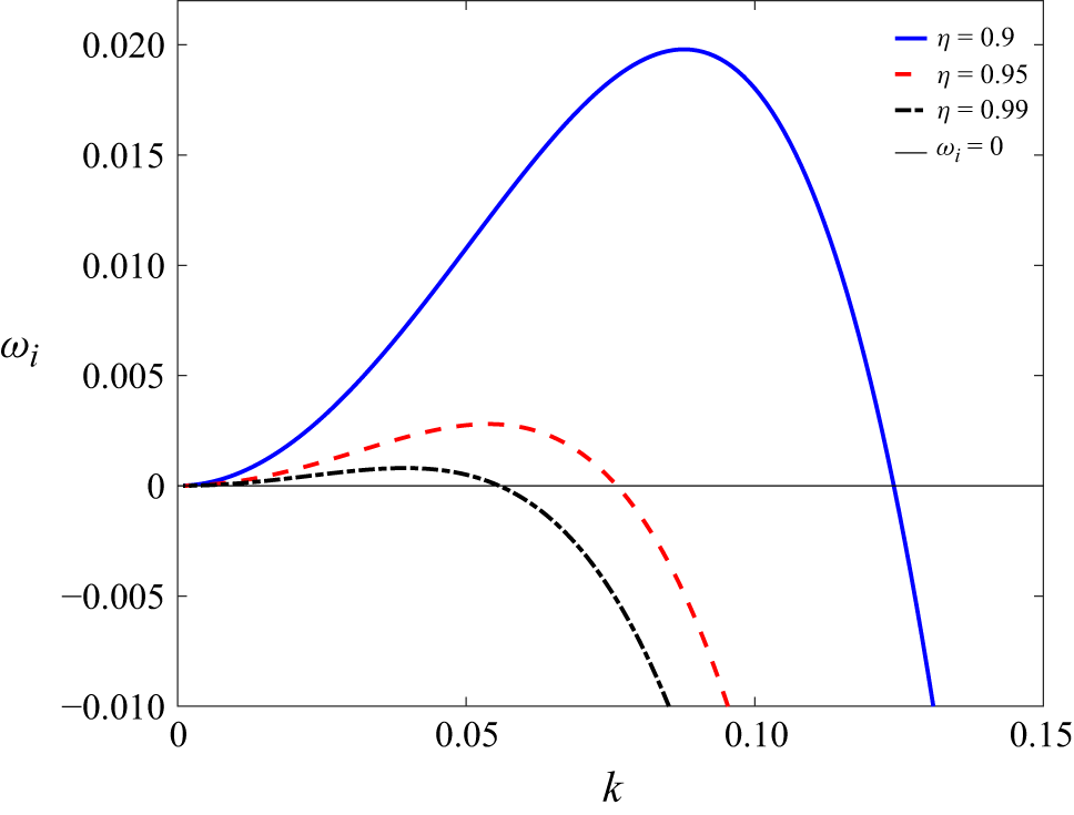
A typical dispersion curve is shown in figure 2. The presence of a range of wavenumbers with
 $\omega _i \gt 0$
implies a temporally unstable flow. The role of multiple instabilities due to capillarity, liquid elasticity and thermocapillarity may not be properly gleaned from the dispersion curve. To understand the role of these individual instabilities in introducing temporal instability, the characteristics of functions
 $f_{\textit{Ca}}, f_{W}$
and
 $f_{\textit{Ma}}$
need to be understood. From dispersion relation (4.1), for the elastic, capillary and thermocapillary instabilities to exist, the multiplying functions must possess a positive value and
 $Ma\gt 0$
. From previous studies of Camassa et al. (Reference Camassa, Ogrosky and Olander2014), Patne (Reference Patne2025), the thickness of the ASL will play a pivotal role in introducing temporal and absolute instabilities. Thus, it is imperative to understand the variation of the multiplying functions with the dimensionless ASL thickness (
 $1-\eta$
).
Dispersion curve obtained by using the dispersion relation (4.1) for
 $W=1, Ca=0.001, \tau _a=1, {\textit{Ga}}=0$
and
 $ Ma=1$
. The base flow is unstable for the wavenumber range with
 $\omega _i \gt 0$
.

The variation of perturbation wavespeed (
 $f_0$
) with the scaled ASL thickness (
 $1-\eta$
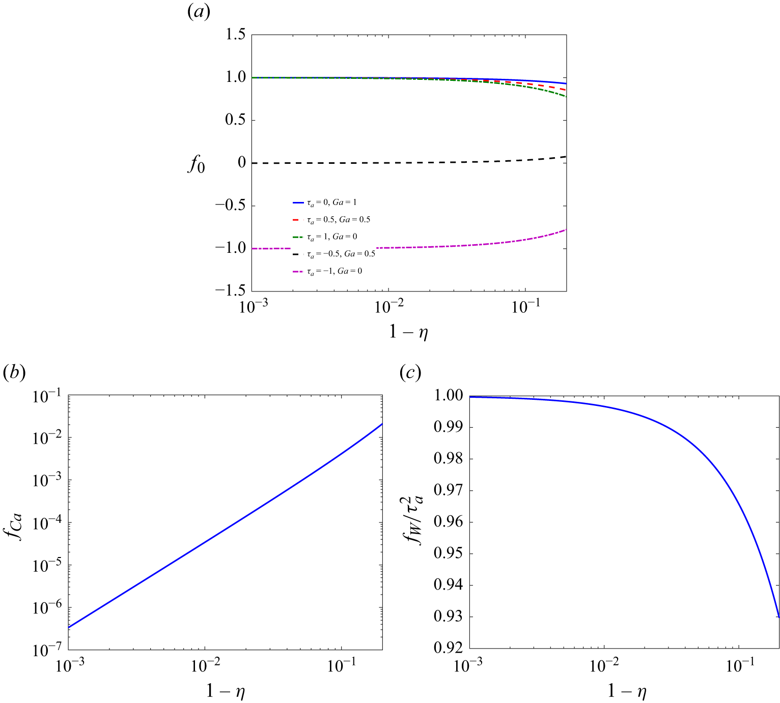
) is shown in figure 3(a). For all parameter combinations of the shear stress exerted by the turbulent air (
 $\tau _a$
) and Galileo number (
 ${\textit{Ga}}$
) relevant to the present study, the wavespeed of the perturbations is positive except for
 $\tau _a=-1$
and
 ${\textit{Ga}}=0$
. The function
 $f_{\textit{Ca}}$
in the capillary term
 $f_{\textit{Ca}}/Ca$
is expected to be a strong function of ASL thickness since an increasing ASL thickness implies an increasing azimuthal curvature effect. Figure 3(b) confirms this conclusion, where the impact of variation in
 $1-\eta$
on
 $f_{\textit{Ca}}$
is shown. An increasing ASL thickness has the opposite effect on the function
 $f_W$
(see figure 3
c), implying the stabilising effect of azimuthal curvature on the ASL elastic instability. Note that we have not shown the variation of
 $f_{\textit{Ma}}$
with
 $1-\eta$
in figure 3 since
 $f_{\textit{Ma}}$
is proportional to
 $f_W$
by a multiplying factor of
 $2 \tau _a^2$
. Thus, figure 3(c) is readily applicable for
 $f_{\textit{Ma}}$
, albeit with the reduction in the magnitude. These features of
 $f_{\textit{Ca}}, f_W$
and
 $f_{\textit{Ma}}$
are in excellent agreement with the numerical predictions of Patne (Reference Patne2024).
Variation of functions
 $f_0, f_{\textit{Ca}}$
and
 $f_{W}/\tau _a^2$
with the dimensionless thickness of the ASL (
 $1-\eta$
): (a)
 $f_0$
versus
 $1-\eta$
; (b)
 $f_{\textit{Ca}}$
versus
 $1-\eta$
; (c)
 $f_{W}/\tau _a^2$
versus
 $1-\eta$
. Note that positive function values of
 $f_{\textit{Ca}}$
and
 $f_{W}/\tau _a^2$
imply an unstable mode. Panel (a) shows that, except for
 $\tau _a=-1$
and
 ${\textit{Ga}}=0$
,
 $f_0\gt 0$
for all other combinations of
 $\tau _a$
and
 ${\textit{Ga}}$
. Panel (b) shows the decrease in
 $f_{\textit{Ca}}$
with decreasing thickness of ASL, while function
 $f_W$
shows the opposite behaviour, as shown in panel (c).

From (4.2), the capillary function
 $f_{\textit{Ca}}$
and
 $f_{\textit{Ma}}$
are independent of
 $\tau _a$
, implying a lack of dependence of the capillary and thermocapillary instability on the respiration stage. However, also from (4.2),
 $f_W$
is proportional to
 $\tau _a^2$
. Thus, the ASL elastic instability does not depend on the inspiration or expiration. Instead, it is a function of the strength of turbulent airflow. For the elastic instability, this occurs since the base state velocity gradient for a purely gravity-driven flow vanishes at
 $r=r_i$
. Thus, the ASL elastic instability predicted here is solely due to the turbulent shear stress exerted by the airflow.
5. Spatio-temporal stability analysis (
 $\boldsymbol{k_i \neq 0}$
)

While conducting temporal linear stability analysis in § 4, we assumed a complex frequency (
 $\omega = \omega _r + i \omega _i$
) and real wavenumber (
 $k$
). This analysis yielded information about the growth or decay of the perturbations with time (i.e.
 $\omega _i$
). In contrast, the fate of the perturbations in the spatial direction, i.e. in the axial direction, remains unknown. The growth/decay of the perturbations along the axial direction could be obtained by conducting a spatial stability analysis, which treats the wavenumber as a complex number (
 $k=k_r + i k_i$
) and frequency as a real number. Due to the form of the normal modes considered in the present study, a spatially unstable eigenvalue must possess
 $k_i\lt 0$
for a set of parameters and real
 $\omega$
.
To analyse the growth/decay of the perturbations in space and time, we must treat both frequency and wavenumber as complex numbers. To analyse the spatio-temporal stability analysis, one can employ the method of Briggs (Reference Briggs1964), which tracks the formation of the saddle point in the
 $k$
plane formed by
 $k_r$
and
 $k_i$
, and cusp point in the
 $\omega$
plane formed by
 $\omega _r$
and
 $\omega _i$
. For a dispersion relation of the form
 $\omega = {\mathcal F}(k)$
, if there is a first-order saddle point in the
 $k$
-plane, a local Taylor series expansion about the saddle point yields
 $(\omega -\omega _{0})\sim (k-k_{0})^{2}$
. Here,
 $\omega _{0} = \omega _{r0}+i \omega _{i0}$
and
 $k_0=k_{r0}+i k_{i0}$
are the locations of the cusp point in the
 $\omega$
plane and saddle point in the
 $k$
plane, respectively.
Based on the
 $\omega _{i0}$
value, the result of the spatio-temporal stability analysis classifies the temporal instability as absolute or convective instability. If
 $\omega _{i0}\lt 0$
, the flow is convectively unstable, implying that the disturbances will be convected along the flow in the downstream direction. Thus, disturbances have the opportunity to develop only in the downstream direction. In contrast, if
 $\omega _{i0}\gt 0$
, then the flow is absolutely unstable, implying growth of the disturbances both in the upstream and downstream direction from their source point. In the present study, the occurrence of absolute instability could lead to the formation of ASL plugs. Thus, our aim is to investigate the range of parameters where the absolute instability exists.
To determine the saddle point, we differentiate the dispersion relation
 $\omega = {\mathcal F}(k)$
with respect to
 $k$
to obtain the group velocity of the perturbations. The saddle point is located where the group velocity vanishes (Huerre & Monkewitz Reference Huerre and Monkewitz1990; Schmid & Henningson Reference Schmid and Henningson2001). Thus, the solution of the equation
 $ {\partial \omega }/{\partial k}=0$
yields the saddle point locations
 $k_0$
. Here, we employ the Kupfer, Bers & Ram (Reference Kupfer, Bers and Ram1987) method in which only the cusp point formation in the
 $\omega$
-plane is necessary to determine the existence of an absolute instability. To form the cusp point, the movement of the dispersion curve in the
 $\omega$
-plane is tracked for varying
 $k_i$
. If, for a finite
 $k_i$
, the cusp point in the
 $\omega$
-plane possesses
 $\omega _{i0}\gt 0$
and follows causality, then the flow is absolutely unstable. The same procedure has been previously employed by Alhushaybari & Uddin (Reference Alhushaybari and Uddin2019, Reference Alhushaybari and Uddin2020), Patne & Ramon (Reference Patne and Ramon2020), Patne & Chandarana (Reference Patne and Chandarana2023), Patne (Reference Patne2025) to determine the absolute instability in multiphase flows.
To obtain the saddle point, we differentiate the dispersion relation (4.1) with respect to
 $k$
and solve the resulting equation for
 $k$
to obtain three roots
 \begin{align} k_0 &= -\frac {i F_1}{3^{1/3} \varDelta } + \frac {i \varDelta }{2\, 3^{2/3} F_2}, \end{align}
 \begin{align} k_0 &= \frac {(i - \sqrt {3}) F_1}{2\, 3^{1/3}\varDelta } - \frac {(i + \sqrt {3}) \varDelta }{4\, 3^{2/3} F_2}, \end{align}
 \begin{align} k_0 &= \frac {(i + \sqrt {3}) F_1}{2\, 3^{1/3}\varDelta } - \frac {(i - \sqrt {3}) \varDelta }{4\, 3^{2/3} F_2}, \end{align}
where
 \begin{align} \varDelta &= \left (9 f_0 F_2^2 + \sqrt {3} \sqrt {8 F_1^3 F_2^3 + 27 f_0^2 F_2^4}\right )^{1/3}, \end{align}
 \begin{align} F_1 &= f_W \, W + \frac {f_{\textit{Ca}}}{\textit{Ca}} + f_{\textit{Ma}} \, \textit{Ma} , \end{align}
 \begin{align} F_2 &= \frac {r_i^2 \, f_{\textit{Ca}}}{\textit{Ca}}. \end{align}
Among three roots, the first root (5.1a
) is purely imaginary since
 $F_1, F_2$
and
 $\varDelta$
are real numbers, thus a spurious saddle point. The second root (5.1b
) and the third root (5.1c
) have the same values of imaginary and real parts, but the real parts are of the opposite sign, with the second and third roots exhibiting negative and positive real parts, respectively. During the temporal stability analysis, we considered the wavenumber to be a positive real number. Thus, here, we consider third root (5.1c
) for further calculation. To obtain the cusp point
 $\omega _0$
, the third root (5.1c
) is substituted into the dispersion relation (4.1). The effect of capillarity, flow inertia, gravity, fluid and solid elasticity on the existence of absolute instability are elaborated in the following discussion.
Before proceeding further, we will explain the rationale for selecting the specific values of
 $\tau _a$
and
 ${\textit{Ga}}$
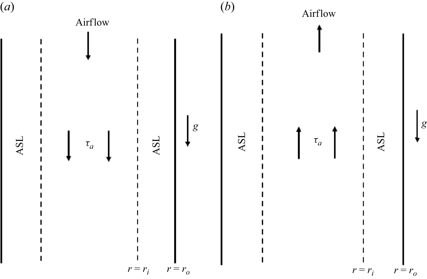
in the subsequent discussion. A schematic of the inspiration and expiration phases is shown in figure 4. During the interval between the successive breathing cycles, the air in the lungs exhibits negligible motion. Thus, the turbulent airflow-induced stress is minimal, and the gravity force will dictate the stability of the ASL, implying
 ${\textit{Ga}}=1$
and
 $\tau _a=0$
due to purely gravity-driven ASL flow.
Schematic of (a) inspiration and (b) expiration phases in the breathing cycle. For the interval between successive breathing cycles
 $\tau _a=0$
, thus, only gravity is relevant.

As the inspiration begins, the velocity of the airflow rapidly increases, and the velocity scale for the non-dimensionalisation includes gravity and turbulent air-driven ASL flow. Due to this,
 ${\textit{Ga}}$
value decreases, while
 $\tau _a$
value increases as inspiration proceeds towards peak value. At the peak of inspiration,
 $|\tau _a^*| \sim O(10^{-2}-1)$
depending on the airway generation, with the lowest
 $|\tau _a^*|$
for tenth generation of the airways and the highest value for the trachea. Using the parameter values given in § 2 yields
 ${\textit{Ga}} \sim O(10^{-2}-0.5)$
with the lowest value for trachea and highest value for the tenth generation. Similarly,
 $\tau _a$
is approximately unity for the trachea and
 $0.5$
for the tenth generation. To account for this phase and range of
 ${\textit{Ga}}$
, we will consider
 ${\textit{Ga}} = 0.5,\tau _a=0.5$
and
 ${\textit{Ga}}=0,\tau _a=1$
parameter combinations. As the inspiration ends, the airflow again has a minimum speed, and parameters
 ${\textit{Ga}}=1$
and
 $\tau _a=0$
become relevant. The same is applicable at the beginning of the expiration phase. As the velocity scale
 $V^*_s$
contains an absolute value of
 $\tau ^*_a$
, the preceding arguments for the values of
 ${\textit{Ga}}$
and
 $\tau _a$
remain applicable for the expiration phase also.
During expiration, the turbulent airflow opposes the gravity-driven flow. As the expiration phase peaks, the airflow speed reaches a maximum, corresponding to the parameters
 ${\textit{Ga}} = 0.5,\tau _a=-0.5$
and
 ${\textit{Ga}}=0,\tau _a=-1$
. As the expiration phase nears the end, the airflow speed decreases to return to the nearly quiescent state between the successive breathing cycles where the gravity-driven flow dominates, for which the curve for
 ${\textit{Ga}}=1$
and
 $\tau _a=0$
again becomes relevant. Without the gravity effect, i.e.
 ${\textit{Ga}}=0$
, the inspiration and expiration phase airflow are indistinguishable. Thus, the results for the parameter combination
 ${\textit{Ga}}=0,\tau _a=1$
and
 ${\textit{Ga}}=0,\tau _a=-1$
turn out to be the same. To conclude, we will consider the results for parametric combinations
 ${\textit{Ga}}=1,\tau _a=0$
for a purely gravity-driven flow,
 ${\textit{Ga}}=0,\tau _a=1$
for a purely turbulent air-driven flow relevant to first few generation of airways, and
 ${\textit{Ga}}\neq 0.5,\tau _a=0.5$
and
 ${\textit{Ga}} =0.5,\tau _a=-0.5$
for the combined gravity- and turbulent air-driven flow, relevant to higher generation of proximal airways, in the subsequent analysis. These parametric combinations will cover the different phases during a complete breathing cycle. The curves for various generations of proximal airways lie between the curves for parameters
 ${\textit{Ga}}=0,\tau _a=1$
and
 ${\textit{Ga}}=0.5,\tau _a=0.5$
for inspiration. Similarly, for expiration, the curves lie between the curves for
 ${\textit{Ga}}=0,\tau _a=1$
and
 ${\textit{Ga}}=0.5,\tau _a=-0.5$
. This allows us to consider airway generations and different phases during the breathing cycle.
5.1. Effect of capillarity
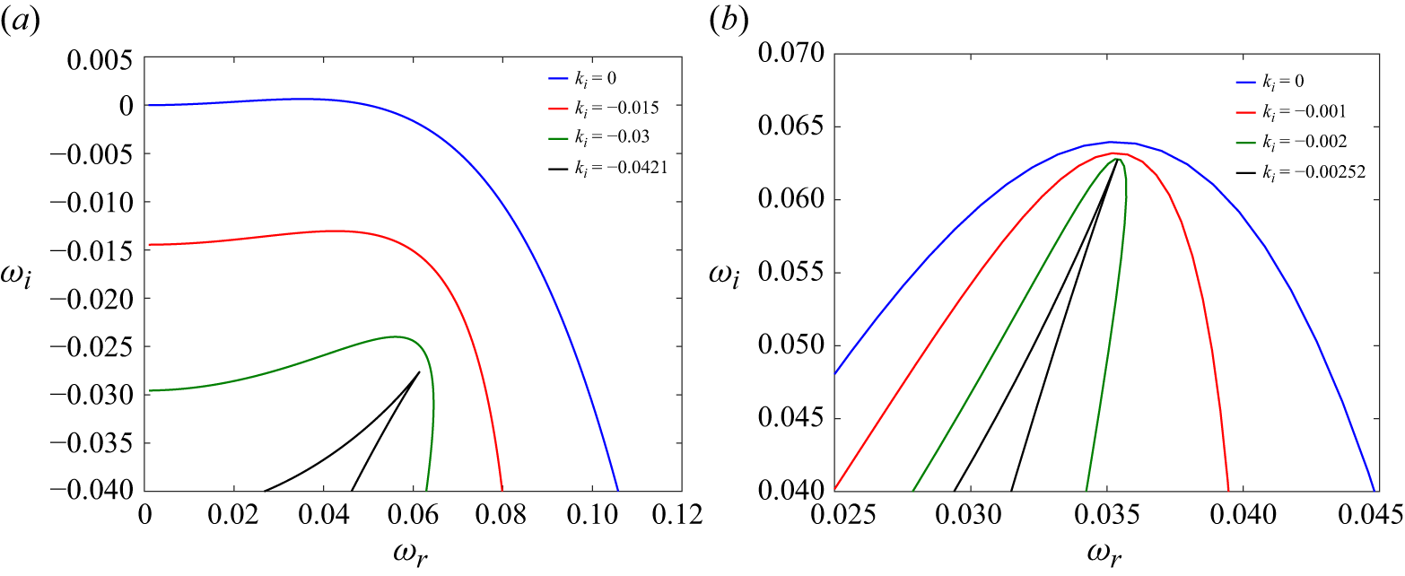
After determining the cusp point using the method of Kupfer et al. (Reference Kupfer, Bers and Ram1987), we must ascertain the ‘genuine nature’ of the cusp point, i.e. adherence to the causality principle as follows. Consider cusp point formation for a set of parameters as shown in figure 5(a). From dispersion relation (4.1), the flow is temporally unstable for an arbitrary
 ${\textit{Ca}}$
for
 $ W=0, {\textit{Ga}}=0$
and
 $\eta =0.95$
. First, we plot the temporal stability analysis curve (corresponding to
 $k_i=0$
and varying
 $k_r$
) in the
 $\omega$
-plane, shown as a black line in figure 5(a). Next, we plot a curve by considering a non-zero negative
 $k_i$
and varying
 $k_r$
. This step is repeated until a cusp point forms in the
 $\omega$
-plane as shown in figure 5(a). To determine the ‘genuine nature’ of the cusp point, a straight line parallel to the
 $\omega _i$
-axis from the cusp point location is drawn. If the drawn line intersects the temporal curve, i.e. the curve for
 $k_i=0$
, for an odd number of times, then the obtained cusp point is genuine else, an evanescent cusp point (Yeo et al. Reference Yeo, Khoo and Zhao1996, Reference Yeo, Khoo and Zhao1999, Reference Yeo, Khoo and Zhao2001). According to this criterion, the cusp point shown in figure 5(a) is genuine.
Cusp point formation in the
 $\omega$
-plane for select values of the capillary number
 ${\textit{Ca}}$
: (a)
 ${\textit{Ca}}=10^{-3}$
; (b)
 ${\textit{Ca}}=10^{-5}$
. The rest of the parameters are
 $W=0, {\textit{Ga}}=0,{ Ma=0, \tau _a=1}$
and
 $\eta =0.95$
. In panel (a), the cusp point forms at
 $\omega _0=0.0613711 - 0.0276457 i$
corresponding to the saddle point
 $k_0=0.0817881 - 0.0420486 i$
. Since
 $\omega _{i0}\lt 0$
at the cusp point, the flow is convectively unstable. In panel (b), the cusp point location is
 $\omega _0 = 0.0353890 + 0.0627634 i$
corresponding to the saddle point
 $k_0=0.0374715 - 0.0025213 i$
. In this case,
 $\omega _{i0}\gt 0$
, implying an absolutely unstable flow.

In the absence of base flow, the Rayleigh–Plateau or capillary instability is inherently absolutely unstable. The presence of the base flow due to the shearing by turbulent airflow and gravity modifies this scenario. For
 ${\textit{Ca}}=10^{-3}$
, from figure 5(a), at the cusp point
 $\omega _{i0} \lt 0$
. Thus, following Briggs (Reference Briggs1964) and Kupfer et al. (Reference Kupfer, Bers and Ram1987), the flow is convectively unstable. If we decrease the capillary number further to
 $10^{-5}$
, the cusp point exhibits
 $\omega _{i0}\gt 0$
, as shown in figure 5(b). Thus, in the absence of the other effects, owing to the base flow, a sufficiently small value of the capillary number is required for the transition from a convectively unstable flow to an absolutely unstable flow, implying the presence of a critical capillary number
 ${\textit{Ca}}_c$
.
The capillary number
 ${\textit{Ca}}=\mu ^* V_s^*/\varSigma ^*$
is proportional to the velocity scale. Thus, during a breathing cycle,
 ${\textit{Ca}}$
will vary, which could lead to the absolute to convective instability transition and vice versa. Additionally, from the analysis of Camassa et al. (Reference Camassa, Ogrosky and Olander2014), the thickness of the ASL plays a major role in determining plug formation. Thus, in the rest of this section, the results are presented in terms of variation of
 ${\textit{Ca}}_c$
with the dimensionless thickness of the ASL, i.e. (
 $1-\eta$
).
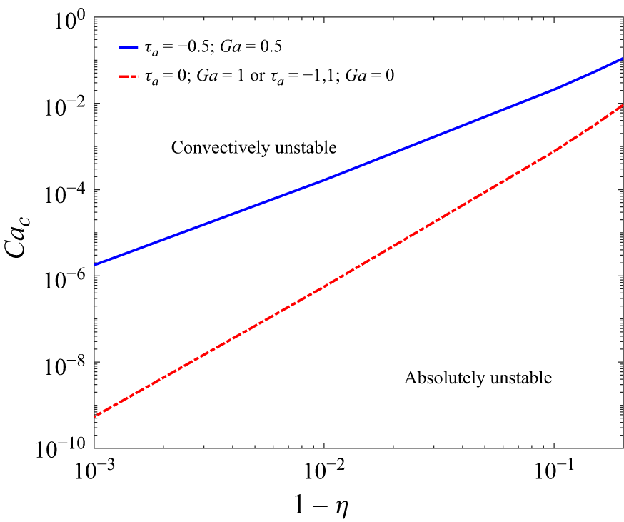
We discuss the results shown in figure 6 by considering a breathing cycle as follows. At the end of expiration and before the beginning of inspiration, the air in the lungs exhibits negligible motion. Thus, the turbulent airflow-induced stress is minimal and the gravity force will dictate the stability of the ASL. For this case, the curve for
 ${\textit{Ga}}=1$
and
 $\tau _a=0$
in figure 6 will be applicable. The curve exhibits
 ${\textit{Ca}}_c \sim (1-\eta )^3$
scaling. For a healthy lung,
 $\eta \approx 0.999$
due to three orders of length scale difference between the radius of the airway lumen and ASL thickness. For a purely gravity-driven flow,
 $V_s^* \sim O(10^{-6}-10^{-4})$
m s−1, implying
 ${\textit{Ca}} \sim O(10^{-6}-10^{-4})$
. Referring to the curve for
 ${\textit{Ga}}=1$
and
 $\tau _a=0$
in figure 6, the flow is convectively unstable. Thus, a purely gravity-driven flow in airways of a healthy lung is convectively unstable, implying the inability of the gravity-driven flow to form ASL plugs.
Variation of the critical capillary number (
 ${\textit{Ca}}_c$
) with the dimensionless thickness of the ASL (
 $1-\eta$
) for
 $W=0$
and
 $Ma=0$
. Note that the curves for
 $\tau _a=0, {\textit{Ga}}=1$
and
 $\tau _a = -1,1, {\textit{Ga}}=0$
nearly overlap. Thus, a single curve has been shown. The curve for
 $\tau _a=-0.5, {\textit{Ga}}=0.5$
exhibits scaling
 ${\textit{Ca}}_c \sim (1-\eta )^2$
, while the other curve exhibits scaling
 ${\textit{Ca}}_c \sim (1-\eta )^3$
. The curve for
 $\tau _a=0.5, {\textit{Ga}}=0.5$
shows a small increase in the absolutely unstable region compared with the curves for
 $\tau _a=0, {\textit{Ga}}=1$
and
 $\tau _a = -1,1, {\textit{Ga}}=0$
.

As the inspiration begins, the velocity of the airflow rapidly increases to reach maximum, and the scale for the non-dimensionalisation switches to the maximum velocity induced by the turbulent airflow. In this case, the curves for
 ${\textit{Ga}}=0.5,\tau _a=0.5$
and
 ${\textit{Ga}}=0,\tau _a=1$
in figure 6 will be relevant. When gravity and turbulent airflow exert comparable influence (
 ${\textit{Ga}}=0.5,\tau _a=0.5$
) during inspiration, the absolutely unstable flow region negligibly increases due to the overlap of the curves for
 ${\textit{Ga}}=0.5,\tau _a=0.5$
and
 ${\textit{Ga}}=0,\tau _a=1$
. As the inspiration ends, the airflow again has a minimum speed, and the curve for
 ${\textit{Ga}}=1$
and
 $\tau _a=0$
becomes relevant. The preceding discussion about gravity-driven remains applicable and thus will not be repeated.
As the expiration phase reaches peak, the airflow speed reaches a maximum, which corresponds to the curve
 ${\textit{Ga}}=0.5,\tau _a=-0.5$
in figure 6. The curve shows the scaling
 ${\textit{Ca}}_c \sim (1-\eta )^2$
and exhibits a much larger absolute instability region than the other curves. As the expiration phase nears the end, the airflow speed decreases to return to the nearly quiescent state between the successive breathing cycles where the gravity-driven flow dominates, for which the curve for
 ${\textit{Ga}}=1$
and
 $\tau _a=0$
becomes relevant.
From the previous explanation and figure 6, for a healthy lung with
 $\eta = 0.999$
, i.e.
 $1-\eta =0.001$
, the highest
 ${\textit{Ca}}_c \sim 10^{-6}$
for an absolutely unstable flow is during the peak of the expiration phase. For the same phase, using the velocity
 $V_s^*$
, we obtain
 ${\textit{Ca}} \gt 10^{-4}$
. Thus, plug formation due to absolute instability will not occur for a healthy lung. This starkly contrasts with the distal airways, where even a healthy lung can exhibit an absolute instability (Patne Reference Patne2025).
However, pulmonary diseases can substantially increase the thickness of the ASL (Shah et al. Reference Shah, Scott, Knight, Marriott, Ranasinha and Hodson1996). From figure 6, due to increased ASL thickness, the flow can access the absolute instability region at a much higher
 ${\textit{Ca}}$
. This leads to the possibility of plug formation due to absolute instability, particularly during expiration. Clinical observations of Huang et al. (Reference Huang2024) confirm the existence of these plugs in the proximal airways of patients with asthma and the lack of such plugs in healthy lungs, thereby affirming the predictions of the present study.
5.2. Effect of ASL elasticity
The mucus layer in ASL exhibits strong elasticity (Lai et al. Reference Lai, Wang, Wirtz and Hanes2009; Hill et al. Reference Hill2014). In this section, we analyse the impact of ASL elasticity on the occurrence of absolute instability. The result of an increasing elasticity (represented by the Weissenberg number,
 $W$
) on the absolute and convective instability regions in
 $(1-\eta ) - Ca_c$
parametric space is shown in figure 7(a). An increasing
 $W$
leads to a substantial reduction in the convective instability region by leading to the formation of an island of convective instability in parametric space. Thus, even with the low thickness of the ASL and high
 ${\textit{Ca}}$
, the flow can become absolutely unstable, thereby leading to plug formation. For a healthy lung,
 $W\lt 1$
; thus, the ASL elasticity may not play a role in introducing absolute instability in the proximal airways.
Variation of the critical capillary number (
 ${\textit{Ca}}_c$
) with the dimensionless thickness of ASL (
 $1-\eta$
). Panel (a) is for
 ${\textit{Ga}}=0$
and select values of the Weissenberg number
 $W$
. For
 $W=0$
, the absolute and convective instability regions are separated by a straight line. For
 $W \neq 0$
, convective instability exists in the concave region of the curves. Panel (b) is for
 $W=10$
and various combinations of
 $\tau _a$
and
 ${\textit{Ga}}$
.

The presence of mucins and other protein macromolecules in the ASL leads to its elastic nature. A pulmonary disease can increase mucin secretion, thereby increasing ASL elasticity (Lai et al. Reference Lai, Wang, Wirtz and Hanes2009). This leads to an increased relaxation time
 $\lambda ^*$
and hence,
 $W$
. From figure 7(a), this will lead to a smaller convective instability region and enhance the possibility of plug formation. Thus, pulmonary diseases increase plug formation probability not only through the increased thickness, but also through the increased ASL elasticity.
The absolute/convective instability regions for three different phases of the breathing cycle are shown in figure 7(b) for
 $W=10$
. Note that for
 $\tau _a=0$
, the fluid elastic instability has a vanishing growth rate since from (4.2),
 $f_W$
is proportional to
 $\tau _a^2$
. Thus, the fluid elastic instability predicted here is a pure consequence of the shear force exerted by the turbulent airflow and flow induced by gravity does not play any role. Note that even in the absence of shear due to turbulent air, the gravity-driven ASL flow could exhibit a purely elastic instability in the inertialess limit (Hu et al. Reference Hu, Fu, Xing, Yang and Xie2021). The influence of gravity is missing in the function
 $f_W$
due to dropping terms with
 $W$
in the constitutive (2.1d
). As explained at the beginning of this section, retaining such terms leads to a mathematically intractable problem; thus, the simplification. Due to the absence of destabilisation due to gravity, the curve for
 ${\textit{Ga}}=1$
and
 $\tau _a=0$
is not shown in figure 7(b). However, the effect of
 ${\textit{Ga}}$
shown in figure 7(b) is through the
 $\omega _r = k f_0$
since from (4.1),
 $f_0$
depends on
 ${\textit{Ga}}$
. To conclude, gravity does not affect the temporal stability of the fluid elastic instability, but it does have a strong impact on the spatio-temporal stability of the flow. Similar to the capillary instability, the absolute instability region is maximum during the expiration phase of the breathing cycle, implying a maximum probability of plug formation during the expiration phase.
5.3. Effect of inhaled air temperature
The effect of inhaled air temperature on mucus dynamics in the proximal airways was investigated by Patne (Reference Patne2024). His analysis predicted a strong stabilising effect of the inhaled air if the inhaled air is at a higher temperature than body temperature, and vice versa. In this section, we analyse the impact of inhaled air temperature on absolute instability in the proximal airways.
During the inspiration phase, as the inhaled air travels through airways, the temperature difference between the inhaled air and the airway muscles will be highest in the trachea and lowest in the alveoli sacs due to air losing heat as it travels towards the alveoli sacs. In the alveoli sacs, due to gas exchange and microfluidic flows, the temperature difference between the air and the alveoli surface will drastically decrease. Thus, the air temperature will approach body temperature. During expiration phase, due to air temperature being almost equal to body temperature, the effect of air temperature will become negligible. Additionally, inhaled air can affect the stability of the ASL only in the presence of airflow in airways, implying that a purely gravity-driven flow is irrelevant. Thus, in the subsequent analysis, we will consider the effect of inhaled air temperature only during the inspiration phase.
First, let us consider the case for the inhaled air being at a higher temperature than body temperature corresponding to
 $Ma\lt 0$
and shown in figure 8(a). As expected, the stabilising effect of the thermocapillarity decreases the size of the absolute instability region in
 $(1-\eta ) - Ca_c$
parametric space. This clearly demonstrates that the inhalation of warm air decreases the possibility of airway closure by absolute instability-induced plugs in the proximal airways.
Variation of the critical capillary number (
 ${\textit{Ca}}_c$
) with the dimensionless thickness of ASL (
 $1-\eta$
) for the (a) negative and (b) positive values of Marangoni number (
 $Ma$
). The impact of the inhaled air will exist only during the inspiration phase. Thus, the curves for
 $\tau _a=-1$
are absent in the plots. Also, curves for
 $\tau _a=1, {\textit{Ga}}=0$
and
 $\tau _a=0.5, {\textit{Ga}}=0.5$
and non-zero
 $Ma$
nearly overlap; thus, only one curve is shown.

For
 $Ma\gt 0$
, i.e. inhaled air is at a lower temperature than body temperature, the thermocapillarity aids capillarity in introducing absolute instability as shown in figure 8(b). Akin to the ASL elasticity, due to the inhaled air beyond a certain thickness of the ASL, flow is absolutely unstable for an arbitrary
 ${\textit{Ca}}$
. Even for healthy lungs, there exists an upper value of
 ${\textit{Ca}}$
beyond which the flow will once again become absolutely unstable. Thus, if the inhaled air is colder than body temperature, then it will lead to an increased possibility of ASL plug formation and subsequent airway closure.
5.4. Effect of axial viscous diffusion
In this section, we use evolution (3.12) which includes
 $O (\epsilon ^2)$
correction to understand the impact of axial viscous diffusion on the occurrence of absolute instability. Similar to evolution (3.8a
), we first scale out
 $\epsilon$
from evolution (3.12) and derive the dispersion relation. This procedure yields the dispersion relation
 \begin{equation} \omega =k f_0 +i \, k^2 \, \left [f_W \, W + \frac {f_{\textit{Ca}}}{\textit{Ca}} + f_{\textit{Ma}} \, Ma \right ] + f_v k^3 - i\, k^4\frac {r_i^2 \, f_{\textit{Ca}}}{\textit{Ca}}, \end{equation}
where
 \begin{eqnarray} f_v = -\frac {2 (r_i - r_o) (d_1 - d_2) + 3 r_i (d_3 + d_4 + d_5) (\log r_i - \log r_o)}{144 r_i^3}, \end{eqnarray}
and
 \begin{align}& d_1 = \textit{Ga} \left(119 r_i^5 + 2 r_i^4 r_o - 70 r_i^3 r_o^2 + 9 r_i r_o^4\right)\!, \end{align}
 \begin{align}& d_2 = \left(27 r_i^5 + r_i^3 (2 - 9 r_o) r_o + 9 r_o^4 - r_i^2 r_o^2 (70 + 9 r_o) + r_i^4 (119 + 27 r_o)\right) \tau _a, \end{align}
 \begin{align}& d_3 = \textit{Ga} \left(-103 r_i^5 + 48 r_i^4 r_o + 12 r_i^3 r_o^2 + 3 r_i r_o^4\right)\!, \end{align}
 \begin{align}& d_4 = \left(r_i^4 (103 + 24 r_i) - 48 r_i^3 r_o - 12 r_i^2 r_o^2 - 3 r_o^4\right) \tau _a, \end{align}
 \begin{align}& d_5 = 36 r_i^4 \bigl(\textit{Ga} r_i - \tau _a\bigr) \bigl(\log r_i - \log r_o)\bigr). \end{align}
The other functions are the same as given in (4.2). An immediate observation of the dispersion relation (5.2) indicates that the axial viscous diffusion does not affect the growth rate of the temporal instability, i.e.
 $\omega _i$
. This feature is in agreement with the predictions of Camassa et al. (Reference Camassa, Ogrosky and Olander2014). Also, since the axial viscous diffusion term is of
 $O(k^3)$
, the effect of this term will be weaker than that of the
 $O(k)$
or
 $O(k^2)$
terms. This hypothesis will be tested in the subsequent analysis.
Due to change in the dispersion relation, the saddle points obtained by differentiating dispersion relation (5.2) with respect to
 $k$
will also change. Solving
 $ {\partial \omega }/{\partial k}$
for dispersion relation (5.2), we obtain
 \begin{align}& k_0 = - \frac {i f_v}{4 F_2} - \frac {i \left(24 F_1 F_2 - 9 f_v^2\right)}{6 \, 2^{2/3} F_2 \varDelta } + \frac {i \varDelta }{12 \, 2^{1/3} F_2}, \end{align}
 \begin{align}& k_0 = - \frac {i f_v}{4 F_2} + \frac {i (1 + i \sqrt {3}) \left(24 F_1 F_2 - 9 f_v^2\right)}{12 \, 2^{2/3} F_2 \varDelta } - \frac {i (1 - i \sqrt {3}) \varDelta }{24 \, 2^{1/3} F_2}, \end{align}
 \begin{align}& k_0=- \frac {i f_v}{4 F_2} + \frac {i (1 - i \sqrt {3}) \left(24 F_1 F_2 - 9 f_v^2\right)}{12 \, 2^{2/3} F_2 \varDelta } - \frac {i (1 + i \sqrt {3}) \varDelta }{24 \, 2^{1/3} F_2}, \end{align}
where
 \begin{align} \varDelta &= \left (\delta _1+\delta _2\right )^{1/3}, \end{align}
 \begin{align} \delta _1 &= 432 \, f_0 F_2^2 + 216 \, F_1 F_2 f_v - 54 f_v^3, \end{align}
 \begin{align} \delta _2 &=\left [ 4 \left(24 F_1 F_2 - 9 f_v^2\right)^3 + \left(432 \, f_0 F_2^2 + 216 \, F_1 F_2 f_v - 54 f_v^3\right)^2 \right ]^{1/2}. \end{align}
Similar to the case for
 $f_v=0$
, among three roots, first root (5.9a
) is purely imaginary, and second root (5.9b
) and third root (5.9c
) have the same values of imaginary and real parts. However, the real parts are of the opposite sign, with the second and third roots exhibiting negative and positive real parts, respectively. Here, we consider third root (5.1c
) for further calculation. During our analysis, we found that the axial viscous diffusion has an increasingly stronger effect for an increasing ASL thickness. For a healthy lung with
 $1-\eta \approx 0.001$
, the effect of axial viscous diffusion is negligible in all phases of the breathing cycle. Thus, in table 3, we consider
 $\eta =0.8$
and compute
 ${\textit{Ca}}_c$
values with/without
 $f_v$
. An immediate conclusion by comparing the last two columns of table 3 is the increase in
 ${\textit{Ca}}_c$
values due to inclusion of axial viscous diffusion during the expiration phase of the breathing cycle and opposite for the other phases. An increase in
 ${\textit{Ca}}_c$
and associated increase in the absolute instability region during the expiration phase is shown in figure 9. From table 3 and figure 9, the effect of axial viscous diffusion is not dramatic. As hypothesised previously, this could be due to the
 $f_v$
term being
 $O(k^3)$
, while instabilities are longwave which diminishes the effect of axial viscous diffusion.
Effect of axial viscous diffusion on the critical capillary number (
 ${\textit{Ca}}_c$
) for
 $Ma=0, \eta =0.8$
and
 $W=0$
. The table shows an increase in
 ${\textit{Ca}}_c$
during the expiration phase due to axial viscous diffusion and a small decrease during other phases.

Variation of critical capillary number (
 ${\textit{Ca}}_c$
) with the dimensionless thickness of ASL (
 $1-\eta$
) for
 $W=0, \tau _a=-0.5, {\textit{Ga}}=0.5$
and
 $ Ma=0$
. The figure shows the effect of axial viscous diffusion on the absolute instability region.

6. Summary
Camassa et al. (Reference Camassa, Ogrosky and Olander2014) demonstrated excellent agreement between the experimental observations of plug formation and absolute instability predicted by the long-wave theory-based model for the flow of a Newtonian liquid coating the inner surface of a rigid tube. Their analysis demonstrated that the existence of an absolutely unstable flow is a sufficient condition for plug formation. Note that Tseluiko & Kalliadasis (Reference Tseluiko and Kalliadasis2011), Ishimura et al. (Reference Ishimura, Mergui, Ruyer-Quil and Dietze2023), Dietze (Reference Dietze2024) observed the formation of saturated-amplitude waves in an absolutely unstable film flow as an alternative path to the plug formation in certain parametric regimes, implying that the absolute instability may not be a sufficient condition for plug formation. Thus, to determine the fate of linearly unstable temporal perturbations, nonlinear solution of the evolution equation is essential. However, in the present study, we focus on determining the parametric regime where the absolute instability exists, which may give rise to ASL plugs.
In the proximal airways, a highly viscoelastic ASL coats the interior of the deformable airway wall. Along with gravity, the turbulent airflow also drives the flow of ASL, thereby leading to gravity and turbulent air-driven ASL flow. The conclusions of previous studies regarding absolute instability are not readily applicable to flows in the proximal airways due to neglecting the turbulent airflow, ASL elasticity, cylindrical flow geometry and inhaled air temperature. The present study aims to fill this lacuna by including these effects and probing for the parametric regime in which an absolutely unstable flow exists in the proximal airways, thereby determining the role of various factors in absolute instability-induced plug formation.
Following Camassa et al. (Reference Camassa, Ogrosky and Olander2014), we derive a longwave evolution equation while neglecting the inertial terms due to the extremely low value of the Reynolds number for ASL flow in the proximal airways. The dispersion relation obtained from the evolution equation is then used to analyse the temporal and spatio-temporal stability of the flow. To consider the whole breathing cycle and multiple generations of proximal airways, we considered the results for parametric combinations
 ${\textit{Ga}}=1,\tau _a=0$
for the gravity-driven flow,
 ${\textit{Ga}}=0,\tau _a=1$
for the turbulent air-driven flow, and
 ${\textit{Ga}}=0.5,\tau _a=-1,1$
for the combined gravity and turbulent air-driven flow in our analysis. The curves for various generations of proximal airways lie between the curves for parameters
 ${\textit{Ga}}=0,\tau _a=1$
and
 ${\textit{Ga}}=0.5 , \tau _a=0.5$
for inspiration. Similarly, for expiration, the curves lie between
 ${\textit{Ga}}=0,\tau _a=1$
and
 ${\textit{Ga}}=0.5,\tau _a=-0.5$
.
The temporal stability analysis predicts instability due to capillarity, ASL elasticity and thermocapillarity. The capillary instability caused by azimuthal curvature, coupled with the interface tension, exhibits a decreasing growth rate with decreasing ASL thickness due to diminishing curvature. The instability due to ASL elasticity exhibits opposite behaviour. The thermocapillary instability exacerbates the capillary and elasticity instabilities for colder inhaled air (i.e. air temperature lower than body temperature) and the opposite for warmer inhaled air (i.e. air temperature higher than body temperature).
We use the method of Kupfer et al. (Reference Kupfer, Bers and Ram1987) to analyse the spatio-temporal stability of the ASL flow. The analysis shows that there exists a critical capillary number
 ${\textit{Ca}}_c$
such that for
 ${\textit{Ca}}\lt Ca_c$
, the flow is absolutely unstable. For purely gravity-driven or turbulent air-driven ASL flow of a Newtonian fluid in a rigid tube,
 ${\textit{Ca}}_c \sim (1-\eta )^2$
, where
 $(1-\eta )$
is the dimensionless thickness of the ASL. During inspiration, the turbulent airflow reinforces the gravity-driven flow. This combined flow exhibits a smaller absolute instability region than purely gravity-driven or turbulent air-driven ASL flow, but still exhibits
 ${\textit{Ca}}_c \sim (1-\eta )^2$
scaling. During expiration, the turbulent air opposes the effect of gravity and leads to scaling
 ${\textit{Ca}}_c \sim (1-\eta )^3$
with a much higher absolute instability region than other cases. Thus, there is a higher chance of plug formation during expiration. For the proximal airways in the upper lobes of the lungs, airflow directions will be opposite to that shown in figure 1. This implies that for the proximal airways in the upper lobes of the lungs, ASL plugs are more likely to occur during inspiration.
For a healthy lung with
 $1-\eta \approx 0.001$
, gravity-driven and/or turbulent air-driven ASL flow will not lead to absolute instability since
 ${\textit{Ca}} \gt Ca_c$
throughout the breathing cycle in contradistinction with the distal airways. However, in a diseased lung,
 $(1-\eta )$
could substantially increase due to the increased thickness of the ASL. From scalings
 ${\textit{Ca}}_c \sim (1-\eta )^2$
and
 ${\textit{Ca}}_c \sim (1-\eta )^3$
during inspiration and expiration, respectively, the flow can become absolutely unstable even at high
 ${\textit{Ca}}$
and lead to plug formation.
For a viscoelastic fluid, unlike a straight line separating the absolute and convective instability regions in
 $(1-\eta )-Ca_c$
parametric space for a Newtonian fluid, due to the ASL elasticity, the boundary becomes a nonlinear curve at sufficiently high values of the Weissenberg number (
 $W$
) with the concave portion exhibiting convective instability. The ASL gains elasticity primarily due to the presence of mucins. Pulmonary diseases involving abnormally high secretion of mucins could enhance the ASL elasticity. This could lead to an absolutely unstable flow even at high
 ${\textit{Ca}}$
and an absolutely unstable flow at arbitrary
 ${\textit{Ca}}$
value for sufficiently high ASL thickness. For example, for ASL with
 $W=10$
, the flow is absolutely unstable for
 $1-\eta \gt 0.009$
.
For colder inhaled air, the Marangoni number (
 $Ma$
) assumes positive values. For
 $Ma\gt 0$
, similar to ASL elasticity, the line demarcating the absolutely and convectively unstable regions modifies to a nonlinear curve. This is associated with an increase in the absolute instability region with the absence of
 ${\textit{Ca}}_c$
at a sufficiently high value of
 $(1-\eta )$
. Thus, the flow is absolutely unstable for arbitrary
 ${\textit{Ca}}$
for increased ASL due to disease-induced changes in the ASL. For
 $Ma=10$
, flow is absolutely unstable for
 $1-\eta \gt 0.044$
. Thus, for diseased lungs exhibiting higher thickness of ASL, inhalation of colder air will lead to absolute instability-induced plug formation and subsequent airway closure, implying the detrimental role of colder air inhalation. For warmer inhaled air,
 $Ma\lt 0$
and the absolute instability region shrinks. Thus, warmer air is beneficial for a diseased lung.
The analysis by Dietze (Reference Dietze2024) indicates that the proximal airways (tenth or lower airway generations) are highly unlikely to be occluded by ASL plugs when the ASL elasticity and inhaled air temperature are neglected. The present study affirms this conclusion. Note that Dietze (Reference Dietze2024) assumed laminar airflow even in the proximal airways, unlike the present study. However, our results indicate that if the effect of ASL elasticity and inhaled air temperature are included, then even the proximal airways could be occluded by the ASL plugs. To conclude, the present analysis predicts that while proximal airways in a healthy lung will not have absolutely unstable flow and consequent plug formation, there could be plug formation in the proximal airways of a diseased lung due to cylindrical flow geometry, ASL elasticity and inhaled air temperature. Clinical observations of Huang et al. (Reference Huang2024) showed that the proximal airways in a healthy lung do not exhibit ASL plugs, but in the diseased lung, proximal airways can develop persistent ASL plugs. Thus, the predictions of the present study are in good agreement with clinical observations.
The predictions of the present study could be further quantitatively improved as follows. We have considered a local model incorporating the role of turbulent airflow and rigid airway walls. However, the airway walls are deformable, which could play a role in controlling ASL dynamics. Consideration of the non-local model could further quantitatively improve the predictions. Temporal instabilities responsible for the absolute instability could be stabilised due to the ‘reversing butter-knife effect’ during a breathing cycle (Halpern & Frenkel Reference Halpern and Frenkel2003; Romano et al. Reference Romano, Fujioka, Muradoglu and Grotberg2019). The impact of the time-periodic nature of the base flow could be explored by considering either a transient stability or Floquet method to analyse stability. The present study could be extended to include these effects. The predictions of Tseluiko & Kalliadasis (Reference Tseluiko and Kalliadasis2011), Ishimura et al. (Reference Ishimura, Mergui, Ruyer-Quil and Dietze2023), Dietze (Reference Dietze2024) regarding the formation of saturated-amplitude waves in an absolutely unstable film flow suggest the necessity of tracking the perturbation development to the nonlinear stage to ascertain the relationship between absolute instability and plug formation. Finally, experiments along the lines of Camassa et al. (Reference Camassa, Ogrosky and Olander2014) for a viscoelastic fluid lining the inside of a tube could validate the predictions of the present study.
Supplementary material
Supplementary material is available at https://doi.org/10.1017/jfm.2026.11416.
Funding
R.P. acknowledges financial support from the SERB-DST under grant SRG/2023/000223.
Declaration of interest
The authors report no conflict of interest.
Author contributions
M.P. and S.R. contributed equally.
Appendix A. Evolution equation
The function
 $\mathcal G$
in the longwave evolution (3.8a
) is
 \begin{eqnarray} {\mathcal G}(\zeta ,\partial _Z \zeta ,\partial _Z^2 \zeta ,\partial _Z^3 \zeta ,\partial _Z^4 \zeta ) =-\frac {b_1 \, ( \partial _Z \zeta )^2+b_2 \, \partial ^2 _Z \zeta + b_3 + b_4 \epsilon ^2 r_i^2 \, \partial ^4 _Z \zeta }{16 \, Ca \, \zeta ^3} \end{eqnarray}
and
 $b_1,b_2,b_3$
and
 $b_4$
are
 \begin{align} b_1&=4 \left[ \widehat {\textit{Ca}} \, r_i^2 r_o^2 \bigl(\widehat {\textit{Ma}} - 2 \widehat {W}_m\bigr) + \zeta \left(-2 r_o^2 + \zeta (\zeta (2 + 4 \log r_o - 4 \log \zeta ) \right. \right. \nonumber \\&\quad\left . \left . + \widehat {\textit{Ca}} \, r_i^2 \bigl(\widehat {\textit{Ma}} - 2 \widehat {W}_m\bigr) (-1 - 6 \log r_o + 6 \log \zeta ))\right)\right]\!, \end{align}
 \begin{align} b_2&= r_o^4 + 4 \widehat {\textit{Ca}} \, r_i^2 r_o^2 \bigl(\widehat {\textit{Ma}} - 2 \widehat {W}_m\bigr) \zeta - 4 r_o^2 \zeta ^2 + \zeta ^4 (3 + 4 \log r_o - 4 \log \zeta ) \nonumber \\&\quad - 4 \widehat {\textit{Ca}} \, r_i^2 \bigl(\widehat {\textit{Ma}} - 2 \widehat {W}_m\bigr) \zeta ^3 (1 + 2 \log r_o - 2 \log \zeta ), \end{align}
 \begin{align} b_3 &= 4 r_i^2 \partial _Z \zeta \left[ \widehat {\textit{Ca}} \, r_o^2 \tau _a + \widehat {\textit{Ca}} \, \tau _a \zeta ^2 (-1 - 6 \log r_o + 6 \log \zeta )\right. \nonumber \\&\quad \left . -2 r_o^2 \zeta \bigl(\widehat {\textit{Ca}} \, Ga + \partial ^3 _Z \zeta \bigr) + 2 \zeta ^3 (1 + 2 \log r_o - 2 \log \zeta ) \bigl(\widehat {\textit{Ca}} \, Ga + \partial ^3 _Z \zeta \bigr)\right]\!, \end{align}
 \begin{align} b_4&=r_o^4 - 4 r_o^2 \zeta ^2 + \zeta ^4 (3 + 4 \log r_o - 4 \log \zeta ).\end{align}
Appendix B. Dispersion relation derivation
As discussed in § 5.4, the temporal stability is negligibly affected by the axial viscous diffusion. Thus, we mainly focus on the
 $O(1)$
evolution (3.8a
), while results for the evolution equation with axial viscous diffusion are discussed in § 5.4. Before proceeding with the dispersion relation derivation, we scale back the equations to eliminate
 $\epsilon$
from the evolution equation. This procedure does not modify the structure of the evolution equation. To the eliminate
 $\epsilon$
, we use the transformations
 $Z \rightarrow \epsilon z$
,
 $\tau \rightarrow t \epsilon$
,
 $\widehat {\textit{Ca}} \rightarrow Ca \epsilon ^{-1}$
,
 $\widehat {W} \rightarrow \epsilon W (D\bar v_z)^2$
and
 $\widehat {\textit{Ma}} \rightarrow \epsilon Ma$
. This transforms (A1) to the original variables and parameters.
To obtain the dispersion relation, we linearise the transformed evolution equation by substituting
 $\zeta =r_i + \zeta '$
, where
 $\zeta ' \ll 1$
. This leads to the linearised evolution equation
 \begin{align} &4 \textit{Ca}\, r_i^2 \left[-\left(r_i^2 - r_o^2\right) (2 Ga\, r_i - \tau _a) + 2\, r_i^2 (2 Ga\, r_i - 3 \tau _a)\log (r_i/r_o)\right]\partial _z \zeta \nonumber\\ &\quad - \left[-\left(r_i^2 - r_o^2\right) \left(r_o^2 + r_i^2 (-3 + 4 Ca\, r_i (\textit{Ma} - 2 W))\right)\right] \partial ^2 _z \zeta \nonumber\\ &\quad + \left[4 r_i^4 (-1 + 2 Ca\, r_i (Ma - 2 W)) \log (r_i/ r_o)\right] \partial ^2 _z \zeta\nonumber \\&\quad + r_i^2 \left(-3 r_i^4 + 4 r_i^2 r_o^2 - r_o^4 + 4 r_i^4 \log (r_i/r_o)\right) \partial ^4 _z \zeta + \partial _t \zeta =0. \end{align}
In (B1), we use normal modes
 $\zeta ' = \tilde \zeta e^{i(kz-\omega t)}$
, where
 $k$
and
 $\omega$
are the wavenumber and perturbation frequency, respectively. For the temporal stability analysis,
 $k$
will be treated as a real number, while for frequency, we consider
 $\omega = \omega _r + i \omega _i$
. If
 $\omega _i \gt 0$
, then the flow is temporally unstable. Upon using the normal modes, the dispersion relation leads to (4.1).