1 Introduction
Flow instabilities may be broadly divided into two categories, convective and global. The former involve disturbances that undergo spatial growth as they are convected away from their inception point. In such cases, all regions of the flow eventually return to their equilibrium state, once the disturbance has passed. In parallel or weakly non-parallel frameworks, the dynamics of such flows is underpinned by local, convectively unstable, downstream-travelling modes, such as the Kelvin–Helmholtz (KH) mode, typically observed in free shear layers, or Tollmien–Schlichting (TS) waves, typically observed in boundary layers. Globally unstable flows, on the other hand, involve disturbances that undergo temporal growth throughout the domain.
When analysed locally, global instability generally involves a feedback loop between upstream- and downstream-travelling modes. In free-shear flows, the downstream-travelling mode is frequently a KH instability, whereas the nature of the upstream-travelling mode may vary depending on the flow considered. Powell (Reference Powell1953) proposed that acoustic waves are responsible for the feedback that underpins tonal behaviour observed in underexpanded supersonic jets which screech, a concept later used to explain the tonal dynamics of impinging jets (Krothapalli Reference Krothapalli1985; Krothapalli et al. Reference Krothapalli, Rajkuperan, Alvi and Lourenco1999; Gojon, Bogey & Marsden Reference Gojon, Bogey and Marsden2015; Bogey & Gojon Reference Bogey and Gojon2017; Gojon & Bogey Reference Gojon and Bogey2017) and cavity flows (Karamcheti Reference Karamcheti1956; Rossiter Reference Rossiter1964; Rowley, Colonius & Basu Reference Rowley, Colonius and Basu2002; Yamouni et al. Reference Yamouni, Mettot, Sipp and Jacquin2013). In these flows, upstream disturbances are spatially amplified up to some downstream point at which they undergo an interaction (with a solid surface where impinging jets and cavities are concerned, with shock cells in the case of screeching jets) that causes them to be scattered into, among other things, upstream-travelling sound waves, which are then reflected in the nozzle plane. When the phases of the upstream- and downstream-travelling waves are matched at the boundaries, and the reflection conditions are such that positive gain is possible, one has resonance, as well as global instability.
Towne et al. (Reference Towne, Cavalieri, Jordan, Colonius, Schmidt, Jaunet and Brès2017) showed that, under certain conditions, discrete acoustic modes may be supported within the potential core of a jet, which behaves as a wave guide. Much of the flow physics could be understood using three simplified models: a cylindrical, soft-walled duct; a cylindrical vortex sheet; and a locally parallel, finite-thickness jet. Turning points associated with the narrowing of the potential core were identified at which the guided, propagative acoustic modes become evanescent, whence their reflection into upstream-travelling guided modes that are subsequently reflected in the nozzle plane. The same mechanism was revealed in a global-mode analysis (Schmidt et al. Reference Schmidt, Towne, Colonius, Cavalieri, Jordan and Brès2017), thus explaining the existence of weak tones observed in simulations and experiments (Brès et al. Reference Brès, Jordan, Jaunet, Le Rallic, Cavalieri, Towne, Lele, Colonius and Schmidt2018).
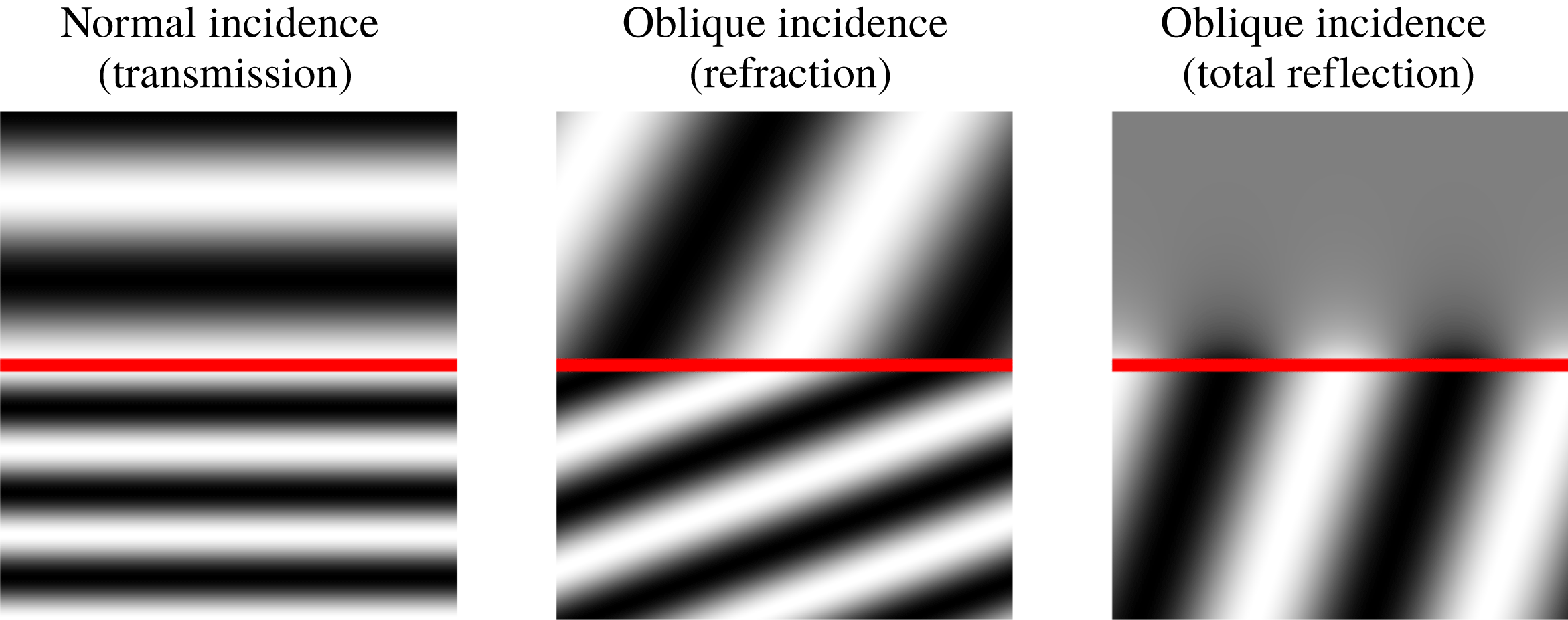
To understand the correspondence between the soft-walled duct model and the vortex-sheet and finite-thickness jet models, properties of the eigenmodes of the latter two were considered. It was thus shown how round jets can support phenomena such as refraction and total reflection (illustrated in figure 1), and how the latter may cause the jet to behave as a wave guide, for both upstream- and downstream-travelling, neutrally stable, acoustic disturbances. Any mechanism enabling interaction between the KH mode and the guided, upstream-travelling acoustic modes, may potentially lead to global instability. Jordan et al. (Reference Jordan, Jaunet, Towne, Cavalieri, Colonius, Schmidt and Agarwal2018) show, for instance, how such interactions underpin tones that occur when a turbulent jet grazes a sharp edge.
Such long-range mechanisms are not the only path to global instability. Wakes (Noack & Eckelmann Reference Noack and Eckelmann1994) and hot jets (Monkewitz & Sohn Reference Monkewitz and Sohn1988) exhibit global instability that is not related to wave reflections, but, rather, to flow features that can be studied in a locally parallel framework. Huerre & Monkewitz (Reference Huerre and Monkewitz1985), adapting the works of Briggs (Reference Briggs1964) and Bers (Reference Bers1975), provide a framework for the study of absolute instability in parallel base flows, showing how the long-time impulse response is dominated by an
 $\exp (-\text{i}\unicode[STIX]{x1D714}_{0}t)$
time dependence, the absolute frequency,
 $\unicode[STIX]{x1D714}_{0}$
, being obtained from a saddle point formed between upstream- and downstream-travelling branches of the dispersion relation. For slowly diverging base flows, the analysis can be extended using asymptotic methods that show how a spatially localised pocket of absolute instability is a requirement for global instability (Chomaz, Huerre & Redekopp Reference Chomaz, Huerre and Redekopp1991; Monkewitz, Huerre & Chomaz Reference Monkewitz, Huerre and Chomaz1993). A recent global stability analysis for slowly diverging base flows, by Siconolfi et al. (Reference Siconolfi, Citro, Giannetti, Camarri and Luchini2017), shows how accurate predictions of global modes may be obtained using the asymptotic approach.
While global stability problems may now be solved numerically (Theofilis Reference Theofilis2011), knowledge of the local mechanisms is frequently necessary, both for a complete understanding of the underlying flow physics, and for the proposition of simplified models. The combination of local and global analyses was the key to understanding the resonant trapped waves in the study of Schmidt et al. (Reference Schmidt, Towne, Colonius, Cavalieri, Jordan and Brès2017).
For both wakes (typically globally unstable) and jets (typically globally stable), the downstream-travelling mode is a KH wave. One may therefore infer that the contrast in stability characteristics of jets and wakes is due to the nature of their upstream-travelling modes, which are often left unexplored. Motivated by the work of Towne et al. (Reference Towne, Cavalieri, Jordan, Colonius, Schmidt, Jaunet and Brès2017), we perform a systematic study of acoustic modes supported by jets and wakes, our ultimate goal being to clarify their role in global instability. We use a parallel double vortex-sheet (DVS) model to provide a general representation of both jets and wakes. We explore the conditions, for both flows, under which trapped acoustic modes may be found, we study the associated physical mechanisms and, finally, we establish the role that these modes play in absolute instability.
While we focus primarily on the incompressible limit, where acoustic modes become evanescent pressure waves, we nonetheless consider certain aspects of the role of compressibility. Specifically, we show how the conditions for spatial stability of propagative acoustic modes in the DVS model are associated with their phase speeds: acoustic modes are neutrally stable when their phase speed is subsonic with respect to the outer flow, and they may be stable or unstable when their phase speed is supersonic, instability being shown to be associated with an influx of fluctuation energy through the vortex sheets. The unstable scenario is shown to correspond to that identified by Tam & Hu (Reference Tam and Hu1989b ).
Illustration of transmission, refraction and total reflection of waves travelling between two media. Reflected waves are not shown in the interest of figure clarity.

The paper is organised as follows. In § 2 we present a double vortex-sheet (DVS) model. Section 3 is concerned with a demonstration of the existence of guided acoustic modes in the DVS and a consideration of the role they play in absolute instability. In § 4 an energy balance approach is used to provide a more complete physical interpretation of the guided acoustic modes; effects of finite impedance are also considered, as is the relation of the guided modes to spatially unstable acoustic modes identified by Tam & Hu (Reference Tam and Hu1989b ) in the supersonic regime. In § 5 we construct the impulse responses of the DVS, and use it to explore compressibility and finite-thickness effects. A closing discussion is provided in § 6.
2 Double vortex-sheet (DVS) flow model
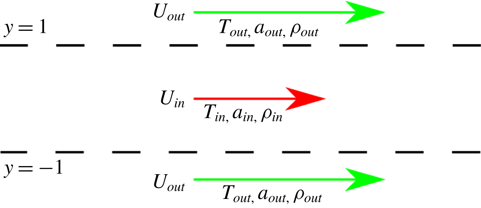
We consider the compressible, linearised Euler equations for a double vortex sheet (DVS) (Lessen, Fox & Zien Reference Lessen, Fox and Zien1965), whose base state is defined as,
 $$\begin{eqnarray}U(y),a(y),T(y),\unicode[STIX]{x1D70C}(y)=\left\{\begin{array}{@{}ll@{}}U_{out},a_{out},T_{out},\unicode[STIX]{x1D70C}_{out},\quad & |y|>1\\ U_{in},a_{in},T_{in},\unicode[STIX]{x1D70C}_{in},\quad & |y|<1,\end{array}\right.\end{eqnarray}$$
where
 $U$
,
 $a$
,
 $T$
and
 $\unicode[STIX]{x1D70C}$
denote, respectively, base-flow velocity, sound speed, temperature and density, subscripts
 $in$
and
 $out$
referring, respectively, to the inner (
 $|y|<1$
) and outer (
 $|y|>1$
) regions, as shown in figure 2. Assuming ideal gas relations, the following parameterisation is obtained,
 $$\begin{eqnarray}\left.\begin{array}{@{}c@{}}U_{in}=-V_{ref},\quad T_{in}=1,\quad a_{in}={\displaystyle \frac{1}{M}},\quad \unicode[STIX]{x1D70C}_{in}=1,\\ U_{out}=1-V_{ref},\quad T_{out}={\displaystyle \frac{1}{T_{r}}},\quad a_{out}={\displaystyle \frac{1}{M\sqrt{T}_{r}}},\quad \unicode[STIX]{x1D70C}_{out}=\unicode[STIX]{x1D70C}_{r}T_{r}.\end{array}\right\}\end{eqnarray}$$
This leads to the following non-dimensional parameters: the Mach number,
 $M$
, the Strouhal number,
 $St=\unicode[STIX]{x1D714}/\unicode[STIX]{x03C0}$
, the inner-to-outer temperature and density ratios, respectively,
 $T_{r}$
and
 $\unicode[STIX]{x1D70C}_{r}$
. The parameterisation is such that the inner fluid properties and the shear strength remain constant. On varying
 $V_{ref}$
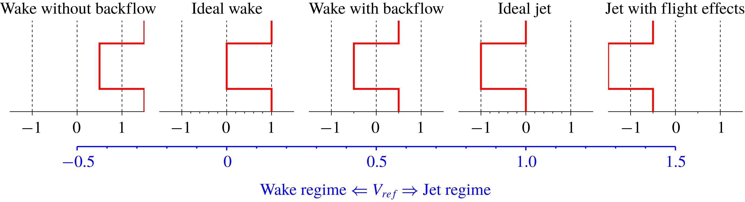
from 0 to 1, the system transitions from an ideal wake to an ideal left-pointing jet, as illustrated in figure 3. But
 $V_{ref}$
can also be considered to define the reference frame in which the flow is observed, thus clarifying a similarity between jets and wakes: they are underpinned by the same physical mechanisms, only observed from different perspectives. Because the choice to consider left-pointing jets, described by
 $V_{ref}=1$
, differs from the more usual convention, according to which jets are considered as right-pointing, wavenumbers and phases speeds associated with jet configurations will be plotted as
 $-\unicode[STIX]{x1D6FC}$
and
 $-c$
in order to facilitate comparison with similar figures found in the literature.
Four regimes can be identified: (i)
 $V_{ref}<0$
, which defines a wake with co-flow; (ii)
 $0<V_{ref}<1$
, defining a wake with reverse flow in the inner region; (iii)
 $V_{ref}=1$
, which corresponds to a left-pointing jet; and, (iv)
 $V_{ref}>1$
, which gives a left-pointing jet with a flight effect. The regime
 $0<V_{ref}<1$
could of course be understood to correspond to a left-pointing jet with counter flow, highlighting the point made above, that differences between jets and wakes are largely due to the choice of reference frame. Also, the limit between ‘wake behaviour’ and ‘jet behaviour’ is arbitrary; we choose, therefore, to refer to
 $V_{ref}<0.5$
as the wake-like regime and
 $V_{ref}>0.5$
as the jet-like regime, and the terms wake and jet are chosen to indicate
 $V_{ref}=0$
and 1, respectively.
The variables of (2.1) are used in all derivations, and those of (2.2) are considered for the study of jet and wake configurations. Small perturbations,
 $u^{\prime }(x,y,t)$
,
 $v^{\prime }(x,y,t)$
and
 $p^{\prime }(x,y,t)$
, are superposed on the base flow,
 $u^{\prime }$
and
 $v^{\prime }$
denoting velocity fluctuations in the streamwise,
 $x$
, and vortex-sheet-normal
 $y$
, directions, respectively,
 $t$
denoting time and
 $p^{\prime }$
denoting pressure fluctuations. The base flow is parallel, and thus homogeneous in the
 $x$
- and
 $t$
-directions, leading to the normal-mode ansatz,
 $$\begin{eqnarray}p^{\prime }(x,y,t)=\hat{p}(y)\text{e}^{\text{i}(\unicode[STIX]{x1D6FC}x-\unicode[STIX]{x1D714}t)},\end{eqnarray}$$
for the pressure, and equivalent expressions for the other flow variables.
Double vortex-sheet (DVS) base flow.

Illustration of the DVS parameterisation defined by (2.2). The flow transitions between wake and jet behaviours with increasing
 $V_{ref}$
.

The inviscid, compressible Euler equations are linearised for the inner and outer regions, giving,
 $$\begin{eqnarray}\displaystyle & \displaystyle \left(\frac{\unicode[STIX]{x2202}^{2}}{\unicode[STIX]{x2202}y^{2}}+\frac{(\unicode[STIX]{x1D714}-U_{in}\unicode[STIX]{x1D6FC})^{2}}{a_{in}^{2}}-\unicode[STIX]{x1D6FC}^{2}\right)\hat{p}_{in}=0, & \displaystyle\end{eqnarray}$$
 $$\begin{eqnarray}\displaystyle & \displaystyle \left(\frac{\unicode[STIX]{x2202}^{2}}{\unicode[STIX]{x2202}y^{2}}+\frac{(\unicode[STIX]{x1D714}-U_{out}\unicode[STIX]{x1D6FC})^{2}}{a_{out}^{2}}-\unicode[STIX]{x1D6FC}^{2}\right)\hat{p}_{out}=0, & \displaystyle\end{eqnarray}$$
matching conditions between the domains giving,
 $$\begin{eqnarray}\displaystyle & \displaystyle (-\text{i}\unicode[STIX]{x1D714}+\text{i}U_{in}\unicode[STIX]{x1D6FC})^{2}\hat{\unicode[STIX]{x1D702}}=\frac{1}{\unicode[STIX]{x1D70C}_{in}}\frac{\unicode[STIX]{x2202}\hat{p}_{in}}{\unicode[STIX]{x2202}y}, & \displaystyle\end{eqnarray}$$
 $$\begin{eqnarray}\displaystyle & \displaystyle (-\text{i}\unicode[STIX]{x1D714}+\text{i}U_{out}\unicode[STIX]{x1D6FC})^{2}\hat{\unicode[STIX]{x1D702}}=\frac{1}{\unicode[STIX]{x1D70C}_{out}}\frac{\unicode[STIX]{x2202}\hat{p}_{out}}{\unicode[STIX]{x2202}y}, & \displaystyle\end{eqnarray}$$
 $$\begin{eqnarray}\displaystyle & \displaystyle \hat{p}_{in}=\hat{p}_{out}, & \displaystyle\end{eqnarray}$$
where
 $\unicode[STIX]{x1D702}$
is the vortex-sheet displacement at
 $y=\pm 1$
. The first two equations match interface displacements between the inner and outer regions, while the third imposes pressure continuity across the vortex sheets. Additionally, it is required that
 $\hat{p}(y)$
be bounded at
 $\pm \infty$
.
Solutions of the system are,
 $$\begin{eqnarray}\hat{p}_{s,a}(y)=\left\{\begin{array}{@{}ll@{}}A_{s,a}\text{e}^{-\unicode[STIX]{x1D709}_{out}y},\quad & y>1\\ \text{e}^{\unicode[STIX]{x1D709}_{in}y}\pm \text{e}^{-\unicode[STIX]{x1D709}_{in}y},\quad & |y|<1\\ \pm A_{s,a}\text{e}^{\unicode[STIX]{x1D709}_{out}y},\quad & y<-1,\end{array}\right.\quad A_{s,a}=\frac{\text{e}^{\unicode[STIX]{x1D709}_{in}}\pm \text{e}^{-\unicode[STIX]{x1D709}_{in}}}{\text{e}^{-\unicode[STIX]{x1D709}_{out}}},\end{eqnarray}$$
with plus and minus signs corresponding to symmetric (
 $s$
) and antisymmetric (
 $a$
) perturbations, where,
 $$\begin{eqnarray}\unicode[STIX]{x1D709}_{in,out}=\sqrt{\unicode[STIX]{x1D6FC}^{2}\left(1-\left(\frac{U_{in,out}-c}{a_{in,out}}\right)^{2}\right)},\end{eqnarray}$$
and
 $c=\unicode[STIX]{x1D714}/\unicode[STIX]{x1D6FC}$
is the streamwise phase velocity. The branch cut of (2.10) is chosen such that
 $-\unicode[STIX]{x03C0}/2\leqslant \arg (\unicode[STIX]{x1D709}_{out,in})<\unicode[STIX]{x03C0}/2$
, as discussed by Tam & Hu (Reference Tam and Hu1989b
). The dispersion relations for the symmetric and antisymmetric modes are, respectively,
 $$\begin{eqnarray}\tanh (\unicode[STIX]{x1D709}_{in})=-\frac{\unicode[STIX]{x1D70C}_{in}}{\unicode[STIX]{x1D70C}_{out}}\frac{\unicode[STIX]{x1D709}_{out}}{\unicode[STIX]{x1D709}_{in}}\left(\frac{U_{in}-c}{U_{out}-c}\right)^{2},\quad \coth (\unicode[STIX]{x1D709}_{in})=-\frac{\unicode[STIX]{x1D70C}_{in}}{\unicode[STIX]{x1D70C}_{out}}\frac{\unicode[STIX]{x1D709}_{out}}{\unicode[STIX]{x1D709}_{in}}\left(\frac{U_{in}-c}{U_{out}-c}\right)^{2},\end{eqnarray}$$
and the other flow variables can be recovered from the pressure distribution as,
 $$\begin{eqnarray}\hat{u} =\frac{\hat{p}}{(c-U)\unicode[STIX]{x1D70C}},\quad \hat{v}=\frac{{\displaystyle \frac{\unicode[STIX]{x2202}\hat{p}}{\unicode[STIX]{x2202}y}}}{\text{i}\unicode[STIX]{x1D6FC}(c-U)\unicode[STIX]{x1D70C}},\quad \hat{\unicode[STIX]{x1D70C}}=\frac{\hat{p}}{a^{2}}.\end{eqnarray}$$
The singularities at
 $c=U_{in,out}$
are avoided by investigating points near, but different from, these singular phase speeds.
3 Acoustic modes and stability of the DVS flow
Our goal is to explore the role of acoustic phenomena in the stability of jets and wakes, considered via the DVS model described in the previous section. What we refer to as acoustic modes are solutions of the convected wave equation,
 $$\begin{eqnarray}{\displaystyle \frac{1}{a^{2}}}\left({\displaystyle \frac{\text{d}}{\text{d}t}}+U{\displaystyle \frac{\text{d}}{\text{d}x}}\right)^{2}p(x,y,t)-\unicode[STIX]{x1D6FB}^{2}p(x,y,t)=0,\end{eqnarray}$$
subjected to appropriate boundary conditions at
 $y\pm 1$
, i.e.
 $p(\pm 1)=0$
or
 $\unicode[STIX]{x2202}p/\unicode[STIX]{x2202}y=0$
on soft- or hard-walled ducts. The model yields a discrete set of acoustic waves, which are guided by the duct. For low frequency solutions of the wave equation are evanescent waves. In the incompressible limit, as
 $a\rightarrow \infty$
, the cut-on frequency that marks transition between evanescent and propagative waves also goes to
 $\infty$
. The evanescent waves that satisfy the wave equation in the incompressible limit are therefore analogous to evanescent-wave solutions that exist for finite
 $a$
, justifying the denomination ‘acoustic’ in reference to solutions in the incompressible limit, which we consider in what follows. For ducts with uniform flow,
 $U$
, a mode with radial wavenumber,
 $n$
, leads to dispersion-relation and group-velocity given by
 $$\begin{eqnarray}\displaystyle & \displaystyle \unicode[STIX]{x1D6FC}=\frac{-U\unicode[STIX]{x1D714}\pm a\sqrt{\unicode[STIX]{x1D714}^{2}-(n\unicode[STIX]{x03C0}/2)^{2}(a^{2}-U^{2})}}{a^{2}-U^{2}}, & \displaystyle\end{eqnarray}$$
 $$\begin{eqnarray}\displaystyle & \displaystyle v_{group}={\displaystyle \frac{\unicode[STIX]{x2202}\unicode[STIX]{x1D714}}{\unicode[STIX]{x2202}\unicode[STIX]{x1D6FC}}}=U+\frac{a}{(c-U)}a, & \displaystyle\end{eqnarray}$$
which will be used throughout the work. Their derivation, along with an overview of duct acoustics, can be found in appendix A.
3.1 Incompressible regime
We now consider the DVS flow in the incompressible limit. We show, firstly, that KH and acoustic-duct modes are asymptotic solutions of the DVS model. We then determine conditions for the existence of acoustic modes in terms of vortex-sheet impedances. This allows us to show how the vortex sheet (VS) may behave in the manner of a hard- or a soft-walled duct, depending on the region of the parameter space that is considered,
In the incompressible limit, equation (2.10) reduces to
 $\unicode[STIX]{x1D709}_{in,out}=\sqrt{\unicode[STIX]{x1D6FC}^{2}}$
. For
 $|a_{r}|\gg 1$
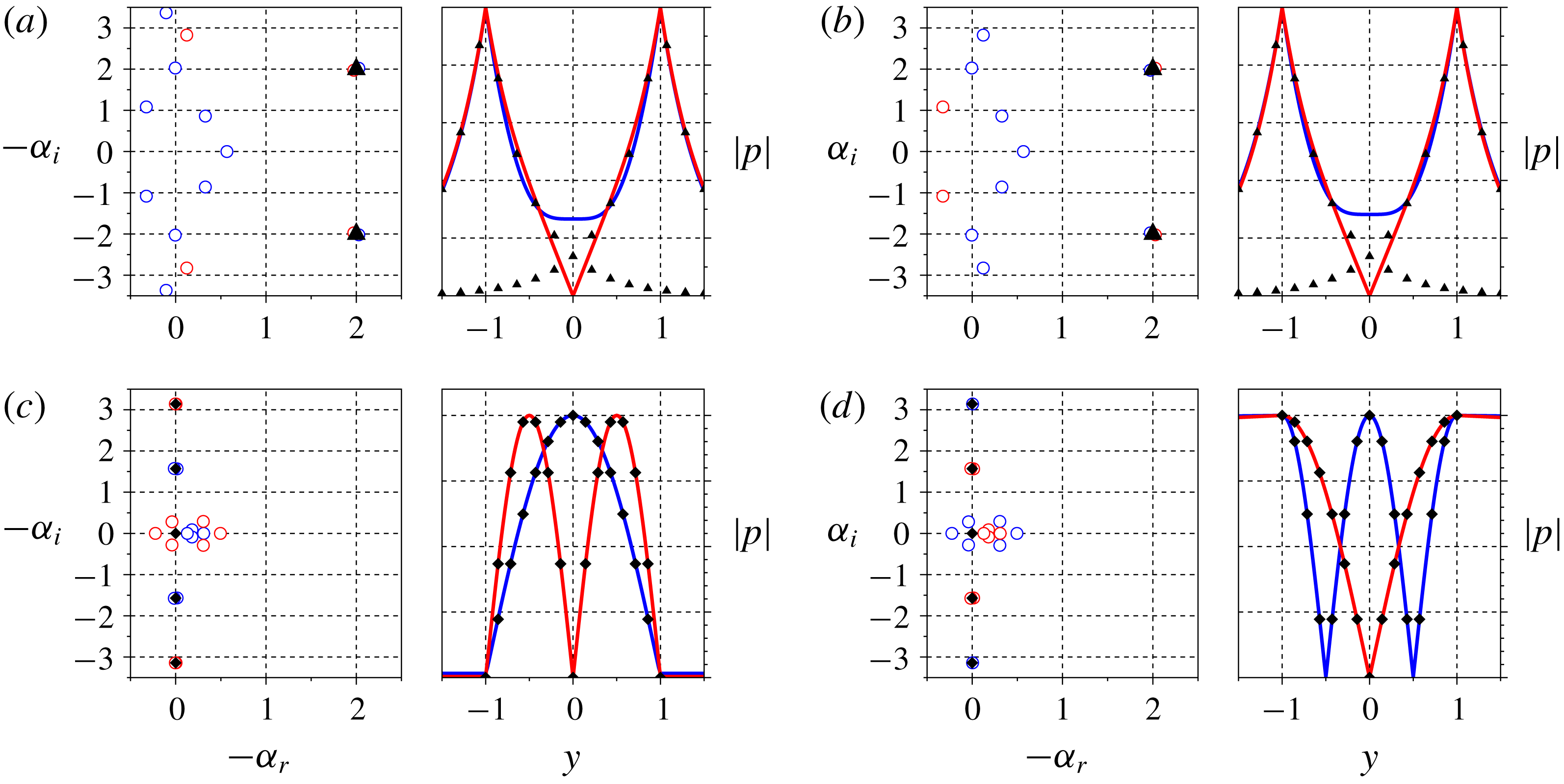
, solutions of the dispersion relation given by (2.11) are KH modes (Lamb Reference Lamb1945, p. 373),
 $$\begin{eqnarray}c=\frac{U_{out}\unicode[STIX]{x1D70C}_{out}+U_{in}\unicode[STIX]{x1D70C}_{in}}{\unicode[STIX]{x1D70C}_{out}+\unicode[STIX]{x1D70C}_{in}}\pm \text{i}\frac{\sqrt{\unicode[STIX]{x1D70C}_{in}\unicode[STIX]{x1D70C}_{out}}}{\unicode[STIX]{x1D70C}_{out}+\unicode[STIX]{x1D70C}_{in}}(U_{out}-U_{in}),\end{eqnarray}$$
which may be symmetric or antisymmetric, as illustrated in figure 4(a,b). Another asymptotic behaviour is obtained when
 $c\approx U_{in}$
or
 $c\approx U_{out}$
:
 $$\begin{eqnarray}\left.\begin{array}{@{}lcl@{}}\text{for}~c\approx U_{in}:\tanh \unicode[STIX]{x1D709}_{in}=0 & \text{and} & \coth \unicode[STIX]{x1D709}_{in}=0\\ \text{for}~c\approx U_{out}:\tanh \unicode[STIX]{x1D709}_{in}=\infty & \text{and} & \coth \unicode[STIX]{x1D709}_{in}=\infty \end{array}\right\}\Rightarrow \unicode[STIX]{x1D709}_{in}=-\text{i}\unicode[STIX]{x03C0}\frac{n}{2}.\end{eqnarray}$$
Solving for
 $\unicode[STIX]{x1D6FC}$
leads to,
 $$\begin{eqnarray}\unicode[STIX]{x1D6FC}^{\pm }=\frac{-U_{in}\unicode[STIX]{x1D714}\pm a_{in}\sqrt{\unicode[STIX]{x1D714}^{2}-\left(\unicode[STIX]{x03C0}{\displaystyle \frac{n}{2}}\right)^{2}(a_{in}^{2}-U_{in}^{2})}}{a_{in}^{2}-U_{in}^{2}},\end{eqnarray}$$
which is the dispersion relation for the acoustics of hard- and soft-walled ducts (3.2). For
 $U_{in}=0$
,
 $\unicode[STIX]{x1D6FC}^{+}$
and
 $\unicode[STIX]{x1D6FC}^{-}$
correspond to left- and right-travelling modes, but if a mean flow is present, the phase and/or group velocities of certain modes may change direction, as discussed in appendix A. Figure 4(c,d) shows the similarity between acoustic modes in ducts and those of the DVS jet and wake. When
 $\unicode[STIX]{x1D714}\approx 0$
we have
 $c=\unicode[STIX]{x1D714}/\unicode[STIX]{x1D6FC}\approx 0$
and so,
 $c\approx U_{in}$
and
 $c\approx U_{out}$
, for the wake and jet, respectively, everywhere in the complex
 $\unicode[STIX]{x1D6FC}$
plane, except near
 $\unicode[STIX]{x1D6FC}=0$
.
Comparison between DVS and KH modes (a,b) and duct-like modes (c,d). Spatial spectra are shown on the left of each panel, with blue and red circles indicating symmetric and antisymmetric DVS modes, respectively, black diamonds acoustic-duct modes and triangles single vortex-sheet KH modes. The right-hand panels show eigenmode comparisons between DVS (solid lines), acoustic-duct modes (diamonds) and single vortex-sheet KH modes (triangles). (a) Incompressible jet,
 $\unicode[STIX]{x1D714}=2.5$
, (b) incompressible wake,
 $\unicode[STIX]{x1D714}=2.5$
, (c) incompressible jet,
 $\unicode[STIX]{x1D714}=0.2$
(d) incompressible wake,
 $\unicode[STIX]{x1D714}=0.2$
.

Motivated by the realisation that soft- and hard-walled duct-like behaviours reflect the vortex-sheet ‘stiffness’, we perform a systematic study of the vortex-sheet impedance,
 ${\mathcal{Z}}_{VS}$
, which will also be useful in identifying total-reflection conditions, as in Towne et al. (Reference Towne, Cavalieri, Jordan, Colonius, Schmidt, Jaunet and Brès2017), when we consider compressible flows. The impedance of a single vortex sheet, located at
 $y=1$
, is calculated. Flows above and below the vortex sheet have properties of the outer and inner flows, respectively. For
 $y<1$
we assume
 $p^{\prime }(x,y,t)=A\hat{p}(y)\text{e}^{\text{i}\unicode[STIX]{x1D6FC}x-\text{i}\unicode[STIX]{x1D714}t}$
, while for
 $y>1$
we enforce the Euler equations,
 $p^{\prime }(x,y,t)=B\text{e}^{-\unicode[STIX]{x1D709}_{out}y+\text{i}\unicode[STIX]{x1D6FC}x-\text{i}\unicode[STIX]{x1D714}t}$
. The two domains are connected with interface conditions identical to those of (2.6)–(2.8), giving,
 $$\begin{eqnarray}{\mathcal{Z}}_{VS}(\unicode[STIX]{x1D714},\unicode[STIX]{x1D6FC})=\left.\frac{p^{\prime }}{v^{\prime }}\right|_{y=1^{-}}=\unicode[STIX]{x1D70C}_{out}\frac{\unicode[STIX]{x1D6FC}}{\text{i}\unicode[STIX]{x1D709}_{out}}\frac{(c-U_{out})^{2}}{c-U_{in}}.\end{eqnarray}$$
The impedance of the inner region,
 ${\mathcal{Z}}_{in}$
, is obtained from the
 $|y|<1$
solutions of (2.9), for symmetric and antisymmetric modes, respectively,
 $$\begin{eqnarray}{\mathcal{Z}}_{in,s}(\unicode[STIX]{x1D714},\unicode[STIX]{x1D6FC})=-\unicode[STIX]{x1D70C}_{in}\unicode[STIX]{x1D6FC}\frac{(c-U_{in})}{\text{i}\unicode[STIX]{x1D709}_{in}}\tanh (\unicode[STIX]{x1D709}_{in}),\quad {\mathcal{Z}}_{in,a}(\unicode[STIX]{x1D714},\unicode[STIX]{x1D6FC})=-\unicode[STIX]{x1D70C}_{in}\unicode[STIX]{x1D6FC}\frac{(c-U_{in})}{\text{i}\unicode[STIX]{x1D709}_{in}}\coth (\unicode[STIX]{x1D709}_{in}).\end{eqnarray}$$
Note that the DVS dispersion relation (2.11) is a compatibility condition between the impedances of the vortex sheet and the inner flow region.
In order to determine whether the vortex-sheet impedance should be considered high or low, a reference impedance is defined. Assuming hard- or soft-walled duct modes (
 $\unicode[STIX]{x1D709}_{in}=-\text{i}n\unicode[STIX]{x03C0}/2$
), the hyperbolic functions in the dispersion relation become either 0 or
 $\infty$
; we thus use the other terms of the dispersion relation to define a reference impedance such that,
 $$\begin{eqnarray}\frac{\unicode[STIX]{x1D70C}_{in}}{\unicode[STIX]{x1D70C}_{out}}\frac{\unicode[STIX]{x1D709}_{in}}{\unicode[STIX]{x1D709}_{out}}\left(\frac{U_{in}-c}{U_{out}-c}\right)^{2}=\frac{{\mathcal{Z}}_{VS}}{{\mathcal{Z}}_{ref}}\approx \left\{\begin{array}{@{}ll@{}}0,\quad & \text{with a soft-duct approximation}\\ \infty ,\quad & \text{with a hard-duct approximation},\end{array}\right.\end{eqnarray}$$
where,
 $$\begin{eqnarray}{\mathcal{Z}}_{ref}(\unicode[STIX]{x1D714},\unicode[STIX]{x1D6FC})=\unicode[STIX]{x1D70C}_{in}\frac{\unicode[STIX]{x1D6FC}}{\text{i}\unicode[STIX]{x1D709}_{in}}(c-U_{in}).\end{eqnarray}$$
The reference impedance depends only on the parameters of the inner region, and thus may be interpreted as an impedance to perturbations in the inner region, to which the vortex-sheet ‘stiffness’ is compared. We are interested in the conditions under which the duct-mode ansatz is self-consistent. A duct-mode ansatz for the DVS is assumed, and the impedance ratio calculated; impedances of 0 and
 $\infty$
indicate self-consistency of the ansatz; large (respectively small), but finite, values indicate that hard- (respectively soft-) walled duct modes are a good approximation for DVS modes.
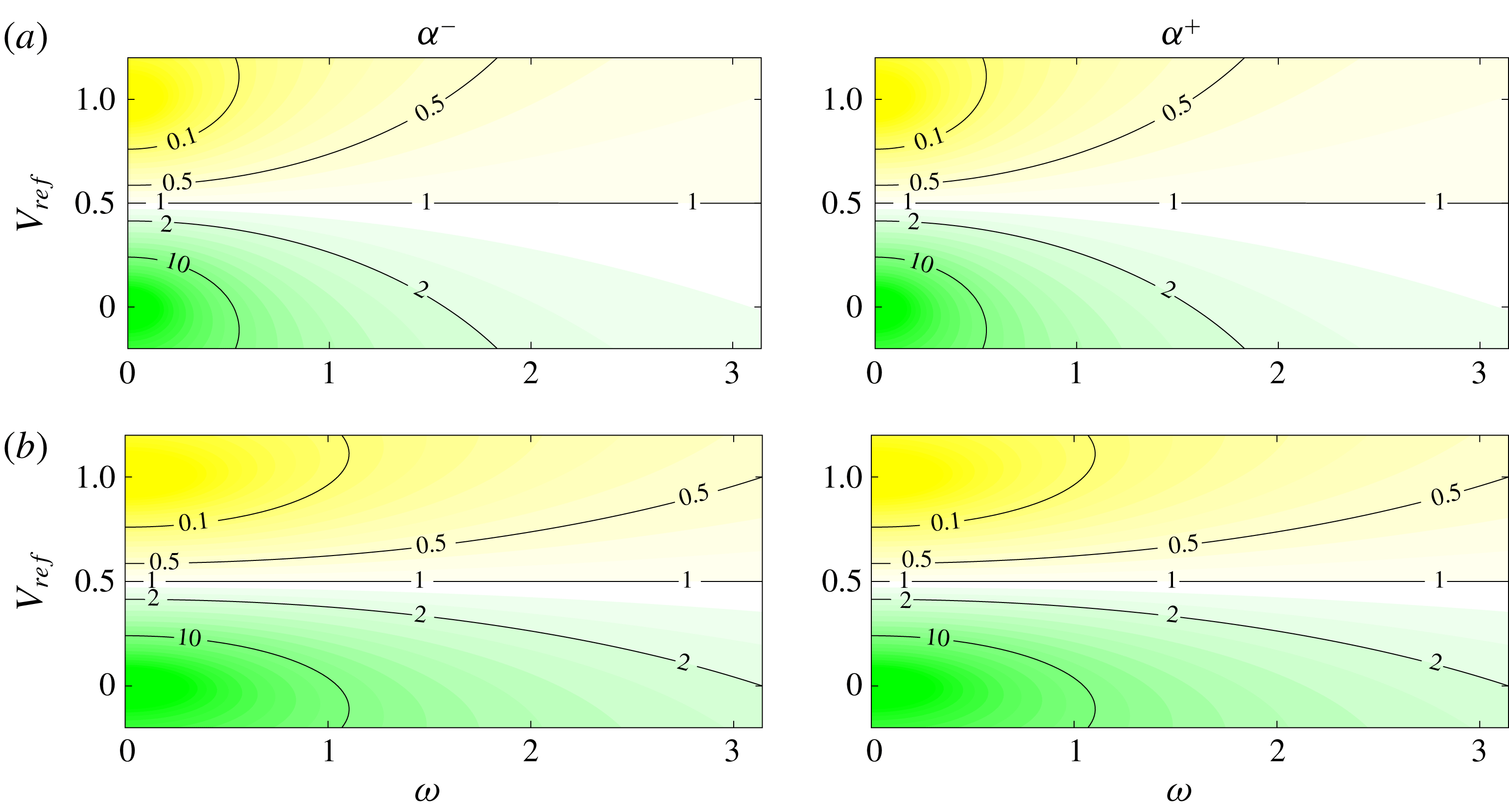
Impedance ratios are shown, as a function of
 $V_{ref}$
and
 $\unicode[STIX]{x1D714}$
, in figure 5. A clear distinction is manifest between jet and wake behaviours at low frequency, low and high values of impedance ratio being observed, respectively, in the jet (
 $V_{ref}=1$
) and wake (
 $V_{ref}=0$
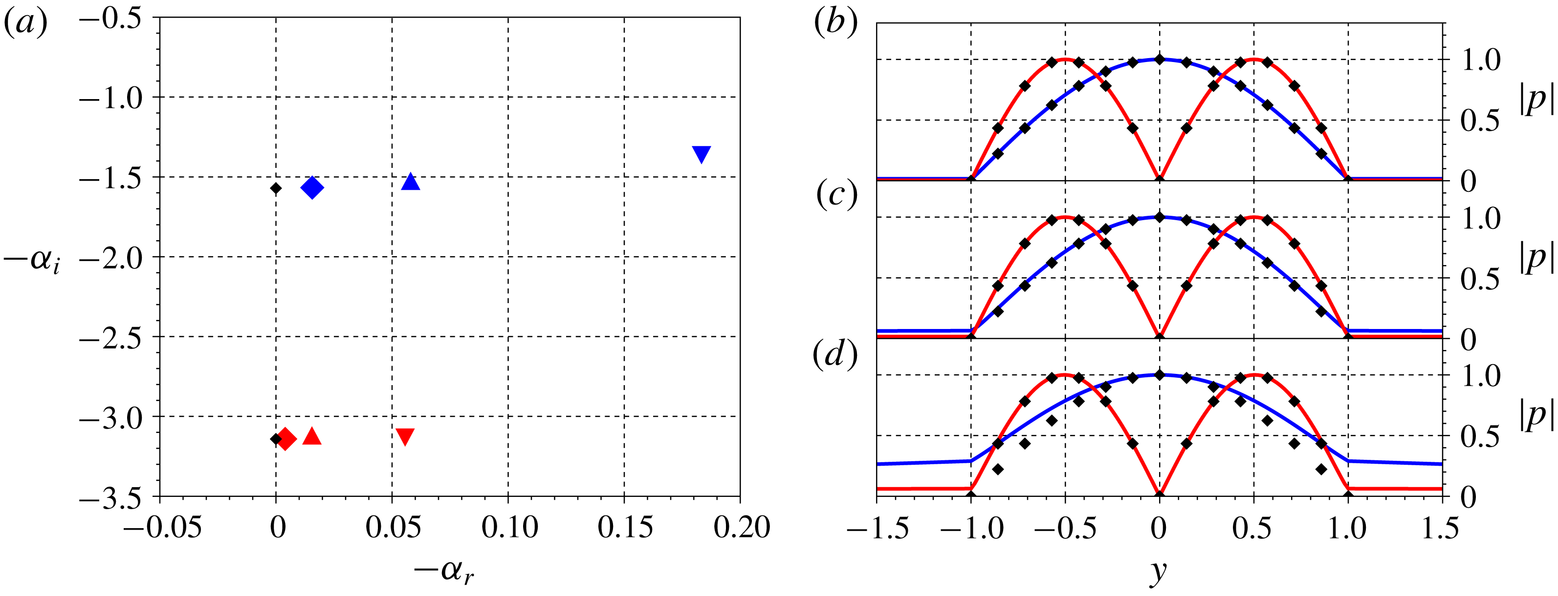
) regimes, satisfying the soft- and hard-walled acoustic-duct ansätze, respectively. At higher frequency the self-consistency condition is weakened, implying a departure from duct-like behaviour, which is manifest in the higher frequency eigenfunctions of figure 6 (cf. DVS mode at
 $\unicode[STIX]{x1D714}=0.8$
for example): when the impedance-ratio values depart from those consistent with the ansatz, the DVS eigenfunctions no longer match, but nonetheless resemble, duct modes, modified to have non-zero support in the outer flow. We may infer that the associated mechanisms are of an acoustic nature, but modified by interaction with the vortex sheets.
We note that the first harmonic duct-like modes of the jet and wake DVS solutions exhibit symmetries similar to those of unstable modes in hot jets (symmetric) and wakes (antisymmetric). This suggests that it is the duct-like modes that provide the upstream-travelling dynamics necessary for absolute instability. The relation between acoustic modes and absolute instability is further explored in what follows.
Impedance-ratio map indicating regions where modes resemble those of soft- (yellow) or hard-walled (green) acoustic ducts. A clear trend is identified at low frequency, wakes (
 $V_{ref}<0.5$
) and jets (
 $V_{ref}>0.5$
) exhibiting hard- and soft-walled behaviours, respectively. The distinction deteriorates at higher frequencies. The colour scale corresponds to absolute value of the impedance ratio (
 ${\mathcal{Z}}_{VS}/{\mathcal{Z}}_{ref}$
) for
 $T_{r}=1$
,
 $\unicode[STIX]{x1D70C}_{r}=1$
,
 $M=0.01$
. (a) and (c) plots correspond, respectively, to first (
 $n=1$
) and second (
 $n=2$
) harmonic, duct-like modes.

Deviation of DVS jet (
 $V_{ref}=1$
) modes from acoustic, duct-like behaviour with increasing frequency. (a) Shows DVS, the markers ♢, ▵, ▿ indicating, respectively
 $\unicode[STIX]{x1D714}=0.2$
, 0.4 and 0.8; (b–d) shows corresponding pressure eigenfunctions, for, from top to bottom,
 $\unicode[STIX]{x1D714}=0.2$
, 0.4 and 0.8, black diamonds indicating the corresponding acoustic-duct mode.

3.2 Absolute instability of incompressible wakes and jets
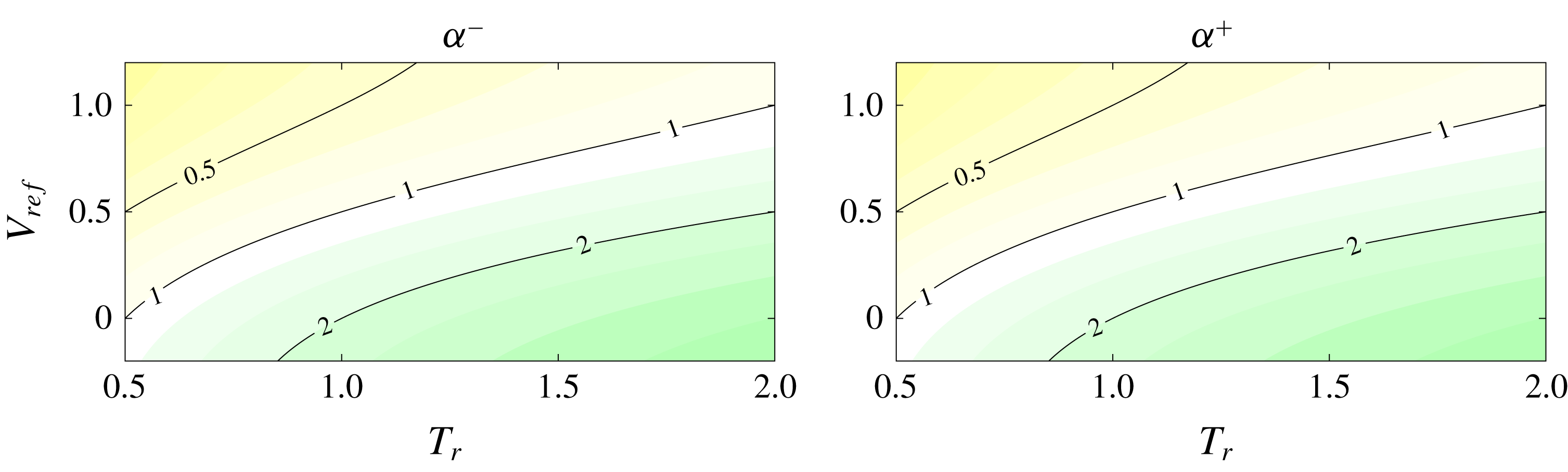
We now wish to establish the relationship between the acoustic duct-like behaviour considered above and the absolute instability of jets and wakes. It is of course clear that, at the DVS saddle point that determines absolute instability, the DVS duct-like modes cannot exactly match true duct modes, as such saddle points do not exist in ducts. Indeed, the results to follow support the idea that a departure from duct-like behaviour is a necessary condition for the onset of absolute instability. We begin with a consideration of the destabilising effect of temperature, when jets are heated and wakes are cooled (Yu & Monkewitz Reference Yu and Monkewitz1990). Figure 7 shows the effect of
 $T_{r}$
on the impedance ratio. This increases with increasing
 $T_{r}$
, but with opposite effects for wakes and jets. When the wake is heated, conditions for duct-like behaviour are improved; when the jet is heated, on the other hand, the duct-like behaviour is degraded. This is a direct consequence of the different duct-behaviour approximations: duct-like behaviour in jets is soft walled, whereas in wakes it is hard walled.
Impedance-ratio (
 ${\mathcal{Z}}_{VS}/{\mathcal{Z}}_{ref}$
) map showing dependence on
 $T_{r}$
and
 $V_{ref}$
. Colour map is the same as in figure 5, for
 $\unicode[STIX]{x1D70C}_{r}=1$
,
 $\unicode[STIX]{x1D714}=\unicode[STIX]{x03C0}/2$
,
 $M=0.01$
, for the first harmonic-duct mode (
 $n=1$
).

We now consider the saddle point that marks the transition between convective and absolute instability. As established by Huerre & Monkewitz (Reference Huerre and Monkewitz1990) for parallel flows, following Briggs (Reference Briggs1964) and Bers (Reference Bers1975), the distinction between absolute and convective instability is given by the imaginary part of the frequency associated with a double root,
 $\unicode[STIX]{x1D6FC}_{0}$
, of the spatial stability problem, such that
 $\unicode[STIX]{x2202}\unicode[STIX]{x1D714}/\unicode[STIX]{x2202}\unicode[STIX]{x1D6FC}(\unicode[STIX]{x1D6FC}_{0})=0$
. The double root must be formed between two modes, one of which is downstream travelling, the other being upstream travelling. Absolute instability can be understood as due to a resonant interaction between modes of opposite group velocities; there is disturbance growth if
 $\text{Im}(\unicode[STIX]{x1D714}_{0})>0$
, where
 $\unicode[STIX]{x1D714}_{0}=\unicode[STIX]{x1D714}(\unicode[STIX]{x1D6FC}_{0})$
. It is known that vortex-sheet models are ill posed, in so far as they present unbounded growth with increasing wavenumber and/or frequency, which precludes calculation of the impulse response. We may nonetheless compute the saddle point, as this permits a useful discussion of the role of the duct-like modes in absolute instability, and we leave discussion of the effects of these on the impulse response to § 5.2.
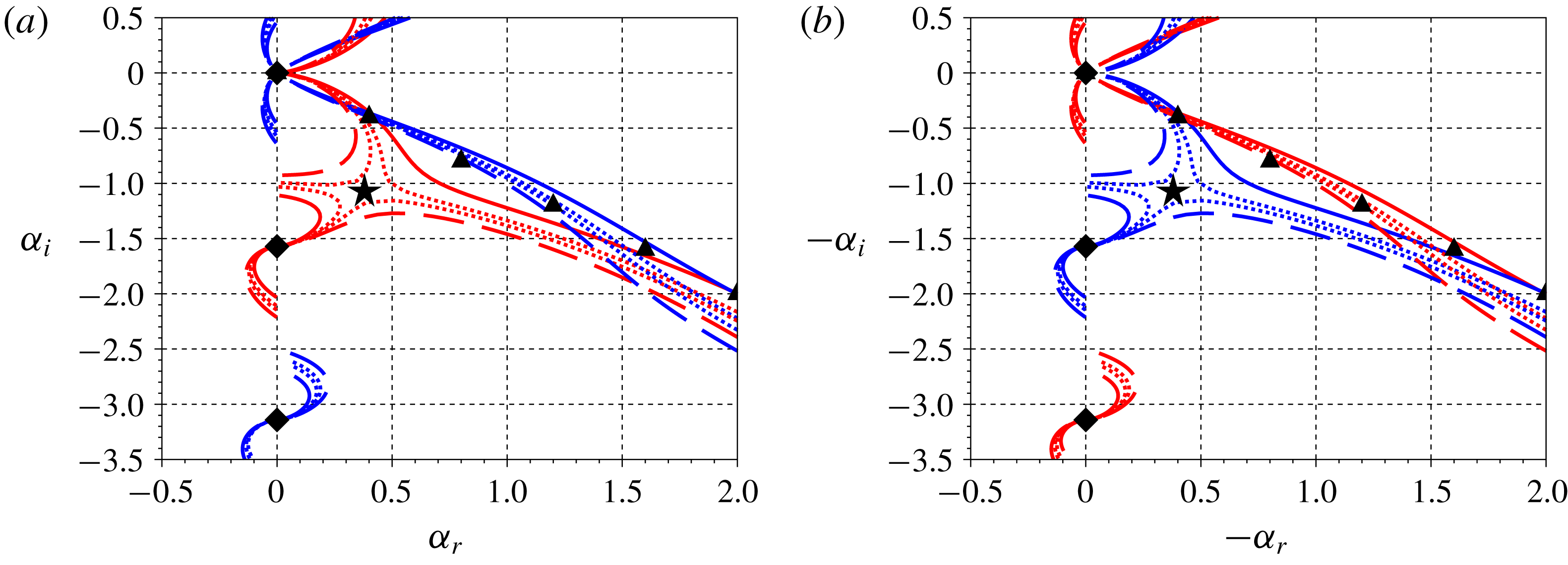
Isothermal DVS jets and wakes are convectively unstable in the absence of co-flow. By varying
 $T_{r}$
and mapping loci of the roots for real frequencies a ‘pinching’ between two branches is observed, indicating a saddle point leaving the negative
 $\unicode[STIX]{x1D714}_{i}$
plane, and signalling the onset of absolute instability. The neutral saddle point for the jet is observed at
 $T_{r}\approx 1.26$
, whereas for the wake it is found at
 $T_{r}\approx 0.79$
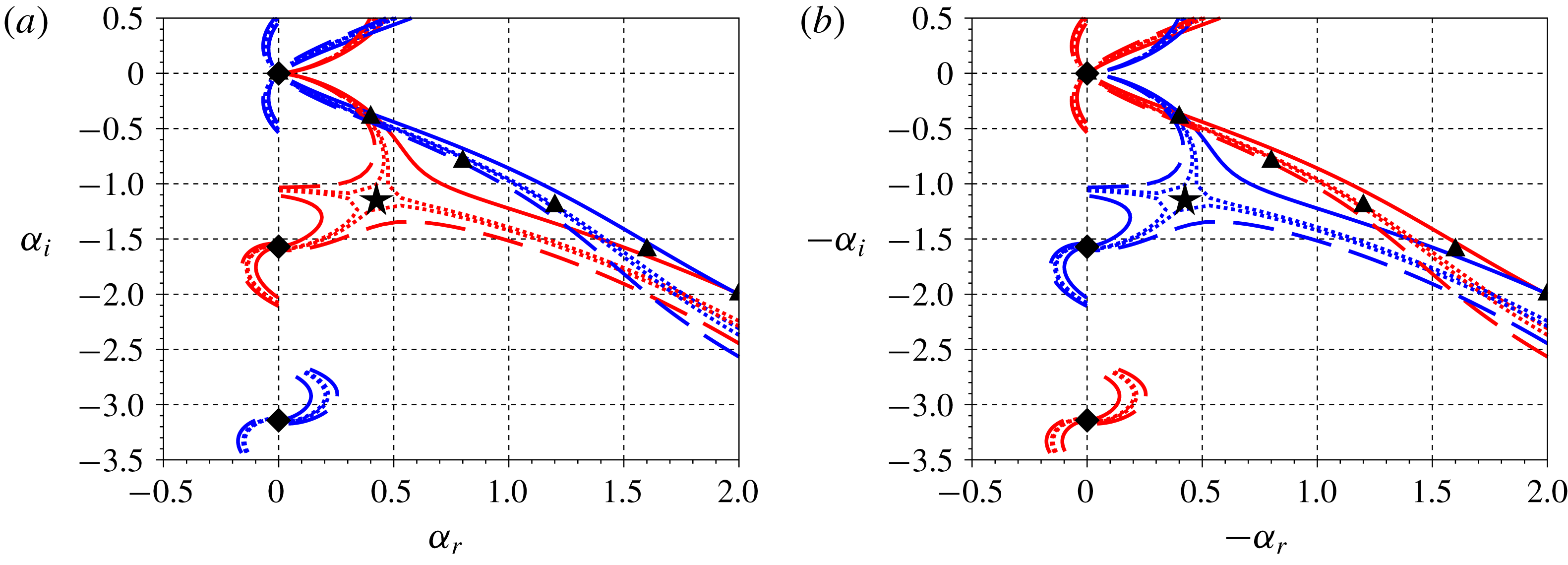
, as shown in figure 8. The branches associated with the saddle point can be recognised as the acoustic and KH branches; this confirms that the acoustic modes underpin absolute instability. Figures 7 and 8 show how destabilisation is associated with a deterioration of the duct-like behaviour. Equivalent results are obtained when the effect of backflow is considered, as can be seen in figures 5 and 9.
Spatial eigenspectra for incompressible (
 $M=0.01$
) wake (a) and jet (b), showing ‘pinching’ of the acoustic and KH branches with temperature variation. Solid, dotted and dashed lines corresponds to
 $T_{r}$
of (1.00, 0.83, 0.76, 0.66) on the left and (1.0, 1.2, 1, 3, 1.5) on the right. Red/blue lines indicate antisymmetric/symmetric modes, diamonds/triangles indicate duct/KH modes. Neutral saddles location with real
 $\unicode[STIX]{x1D714}_{0}$
are found at
 $T_{r}\approx 1.26$
for the jet and at
 $T_{r}\approx 0.79$
for the wake (black stars). Loci are shown for
 $\unicode[STIX]{x1D714}\in [0,1.5\unicode[STIX]{x03C0}]$
.

Same as figure 8, but with saddle point formed due to changes in
 $V_{ref}$
. Solid, dotted and dashed lines corresponds to
 $V_{ref}=(1.00,0.95,0.93,0.90)$
for the jet and
 $(0.00,0.06,0.07,0.10)$
for the wake. Neutral saddles (black stars), are found for
 $V_{ref}=0.935$
and 0.065 for the jet and wake, respectively.

We see how a departure from duct-like behaviour seems to be necessary for interaction between KH and acoustic modes, and therefore for absolute instability. The KH and acoustic branches must move away from their asymptotic loci in order to meet at the saddle point, and with this movement, their eigenfunctions are deformed with respect to their asymptotic forms. This provides the following interesting interpretation of saddle-point ringing: deterioration of the asymptotic duct-mode form involves an extension of the acoustic-mode support across the vortex sheet and into the outer flow, a ‘reaching outward’, while the asymptotic KH deterioration involves a ‘reaching inward’ of the KH mode. The process of absolute instability involves the modes reaching towards one another in order to interact.
3.3 Acoustic modes in the compressible regime
We have seen, in the previous section, how a resonance between KH and acoustic modes underpins the transition to absolute instability in the incompressible regime, under the effects of both
 $V_{ref}$
and
 $T_{r}$
. We now explore some aspects of the compressible regime, where richer dynamics can occur thanks to the existence of propagative waves, both inside and outside the vortex sheet, and the internal trapping of these, as found by Schmidt et al. (Reference Schmidt, Towne, Colonius, Cavalieri, Jordan and Brès2017) and Towne et al. (Reference Towne, Cavalieri, Jordan, Colonius, Schmidt, Jaunet and Brès2017).
The self-consistency impedance condition is extended to incorporate total internal reflection, which also leads to duct-like behaviour. Equation (3.7) shows how, for propagative modes (real
 $\unicode[STIX]{x1D6FC}$
and
 $\unicode[STIX]{x1D714}$
), the impedance is purely imaginary only if
 $\unicode[STIX]{x1D709}_{out}$
is real, which occurs when
 $|c-U_{out}|<a_{out}$
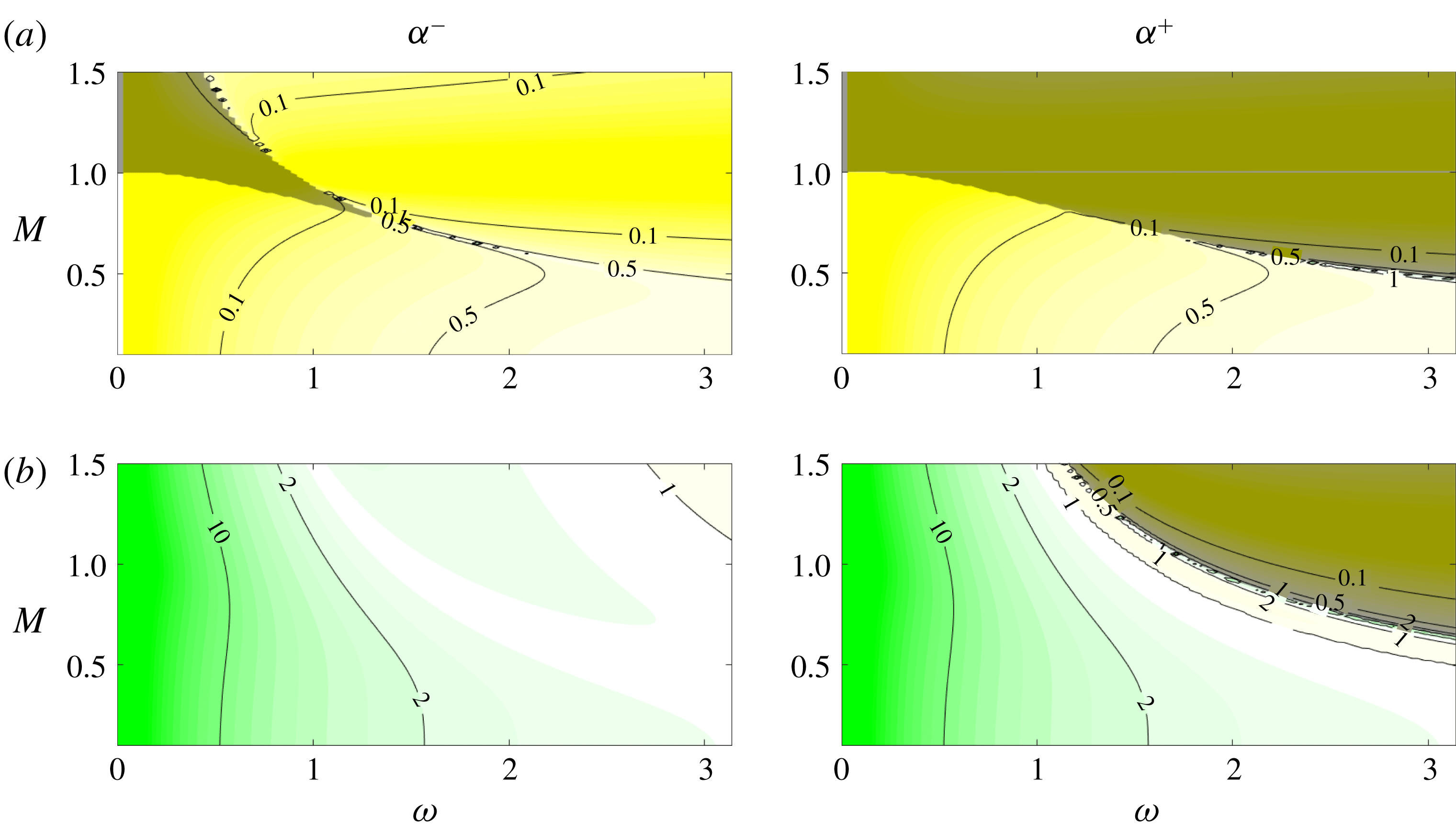
; i.e. when the mode is subsonic, and thus evanescent, in the outer region. As the real part of the impedance is associated with energy flux through the boundary (Rienstra & Hirschberg Reference Rienstra and Hirschberg2018), a purely imaginary impedance implies zero energy flux, due to total internal reflection and an internal trapping of fluctuation energy. A broader discussion of the relationship between impedance and energy flux is provided in § 4.
Figure 10 shows impedance ratios for isothermal jets and wakes. In the shaded regions the impedance is purely imaginary. For a wake, subsonic phase velocity with respect to the outer stream (
 $c$
between
 $1\pm a_{out}$
) is only observed for the downstream-travelling (
 $\unicode[STIX]{x1D6FC}^{+}$
) mode. For the jet, due to the presence of inner flow, both the
 $\unicode[STIX]{x1D6FC}^{+}$
and
 $\unicode[STIX]{x1D6FC}^{-}$
modes may have subsonic phase velocity (
 $c$
between
 $\pm a_{out}$
). This distinction between the jet and the wake suggests that compressibility may have a greater stabilising effect in jets, which will be confirmed in § 5.1, where we consider the impulse response of the DVS.
Impedance-ratio (
 ${\mathcal{Z}}_{VS}/{\mathcal{Z}}_{ref}$
) map showing dependence on
 $\unicode[STIX]{x1D714}$
and
 $M$
. For the jet, both
 $\unicode[STIX]{x1D6FC}^{+}$
and
 $\unicode[STIX]{x1D6FC}^{-}$
modes exhibit total reflection (shaded areas), while for the wake this is only the case for
 $\unicode[STIX]{x1D6FC}^{+}$
(downstream-travelling) modes. The colour map is the same as in figure 5, for
 $T_{r}=1$
,
 $\unicode[STIX]{x1D70C}_{r}=1$
,
 $\unicode[STIX]{x1D714}=\unicode[STIX]{x03C0}/2$
and the first duct mode (
 $n=1$
). (a) Jet (
 $V_{ref}=1$
), (b) wake (
 $V_{ref}=0$
).

3.4 Summary
We have shown how duct-like behaviour is associated with extreme values of vortex-sheet impedance, and how the saddle point underpinning absolute instability is formed by KH and upstream-travelling acoustic branches when the conditions for asymptotic KH and duct-like behaviours are deteriorated. This is consistent with known destabilisation trends associated with temperature ratio, co-flow and compressibility effects, and, furthermore, it clarifies the different symmetries of unstable jet and wake modes. The analysis confirms the essential role played by upstream-travelling acoustic modes in the instability of jets and wakes.
4 Energy balance
We now consider the implications of finite VS impedance. This is done by performing an energy-flux analysis, which also allows us to develop a more complete physical interpretation of the vortex-sheet behaviour. A similar procedure to that applied in § 3.1 is used: duct-mode ansätze are assumed and corresponding impedances and energy fluxes are calculated.
The energy conservation law reads, (Goldstein Reference Goldstein1976; Pierce Reference Pierce1981),
 $$\begin{eqnarray}\frac{\unicode[STIX]{x2202}E}{\unicode[STIX]{x2202}t}+\unicode[STIX]{x1D735}\boldsymbol{\cdot }\boldsymbol{J}=0,\end{eqnarray}$$
where
 $E$
is the total energy and
 $\boldsymbol{J}$
the energy flux. This expression for energy conservation is only valid for small perturbations in uniform flows, and thus will only be applied to control volumes localised in the inner or outer regions. Assuming a stationary regime, where mean energy density is constant in time, equation (4.1) becomes
 $\langle \unicode[STIX]{x1D735}\boldsymbol{\cdot }\boldsymbol{J}\rangle =0$
, where
 $\langle \cdot \rangle$
denotes a time average. The flux is given by,
 $$\begin{eqnarray}\boldsymbol{J}=\left(\frac{a^{2}\unicode[STIX]{x1D70C}^{\prime }}{\unicode[STIX]{x1D70C}}+\boldsymbol{u}^{\prime }\boldsymbol{\cdot }\boldsymbol{U}\right)(\unicode[STIX]{x1D70C}\boldsymbol{u}^{\prime }+\unicode[STIX]{x1D70C}^{\prime }\boldsymbol{U}),\end{eqnarray}$$
which for the no-flow case can be readily identified with the acoustic intensity
 $p^{\prime }\boldsymbol{u}^{\prime }$
. Assuming propagative acoustic modes,
 $\boldsymbol{J}$
components can be written, using (2.12), as,
 $$\begin{eqnarray}\displaystyle & \displaystyle J_{i}(x,y,t)=(\text{Re}(\hat{p}(y)\text{e}^{\text{i}(\unicode[STIX]{x1D6FC}x-\unicode[STIX]{x1D714}t)}))^{2}\frac{1}{\unicode[STIX]{x1D70C}}\left(\frac{1}{c-U}+\frac{U}{a^{2}}\right)\left(\frac{c}{c-U}\right), & \displaystyle\end{eqnarray}$$
 $$\begin{eqnarray}\displaystyle & \displaystyle J_{j}(x,y,t)=\text{Re}(\hat{v}(y)\text{e}^{\text{i}(\unicode[STIX]{x1D6FC}x-\unicode[STIX]{x1D714}t)})\text{Re}(\hat{p}(y)\text{e}^{\text{i}(\unicode[STIX]{x1D6FC}x-\unicode[STIX]{x1D714}t)})\left(\frac{c}{c-U}\right). & \displaystyle\end{eqnarray}$$
The energy balance will be considered in two different manners: (i) a comparison of the magnitude of
 $\boldsymbol{J}$
in the inner and outer regions will be used to justify soft- and hard-walled duct approximations when
 $c\approx U_{out}$
and
 $c\approx U_{in}$
; (ii) a comparison of the energy flux in cross-sections of the inner region and fluxes across the vortex sheets will be used to derive corrections for cases where the impedance is finite.
4.1 Soft- and hard-walled approximations
As we have seen, small and large impedance ratios imply modes that behave as in a duct with uniform flow. In § 3.1 these limits were found when
 $c\approx U_{out}$
or
 $c\approx U_{in}$
. The energy density flux relations defined by (4.2)–(4.4) can be used to clarify the underlying physical mechanisms. The energy flux (4.2) comprises scalar and vector components, in the first and second parentheses, respectively. The former is proportional to
 $c/(c-U)$
and leads to a high magnitude of
 $\boldsymbol{J}$
when
 $c\approx U$
. Pressure continuity requires that the amplitude of the transmitted wave equals the sum of incident- and reflected-wave amplitudes. When
 $c\approx U_{out}$
, the incident wave has a high energy density, and phase opposition of the reflected wave reduces the amplitude of the transmitted wave.
A direct analogy may be drawn with the following simplified model: a wave travelling on a stretched string meets a discontinuity in string density, with the string becoming suddenly much heavier. Here also, reflected waves limit the amplitude at the string discontinuity, which behaves as a rigid constraint. This is analogous to the soft-wall condition, string displacement playing the role of acoustic pressure in the DVS. Similarly, the case where
 $c\approx U_{in}$
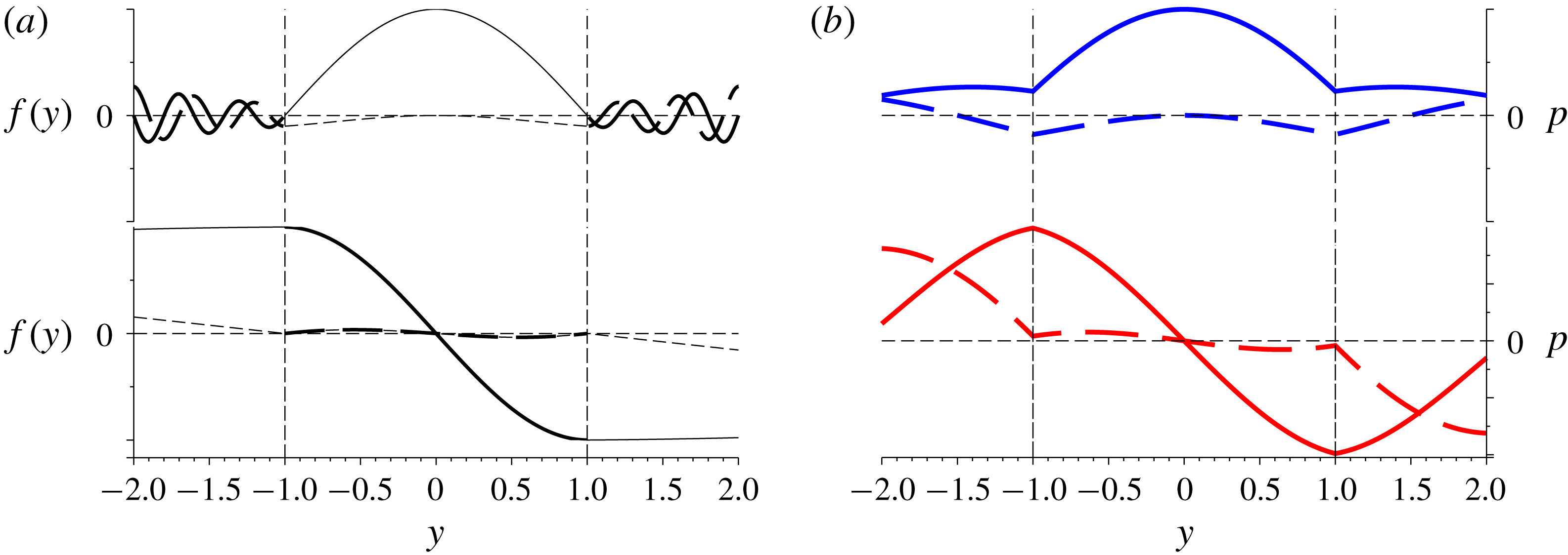
is analogous to a string discontinuity at which the string becomes much lighter. In-phase reflection limits stresses at the discontinuity: a force-relieving boundary condition exists, and outgoing waves, travelling on the light string, have insignificant energy content, and thus only slightly damp oscillations of the heavy string. These analogies are illustrated in figure 11, and the corresponding formulations are provided in appendix C.
Analogy with vibration of an infinite string with DVS modes. (a) Shows an infinite, vibrating string with discontinuous density, the thick line indicating higher density. (b) Show duct-like modes of the jet (top) and the wake (bottom) for
 $\unicode[STIX]{x1D714}=0.8$
. Solid and dashed lines indicate the real and imaginary parts of the eigenfunctions, respectively.

4.2 Energy balance in the inner region
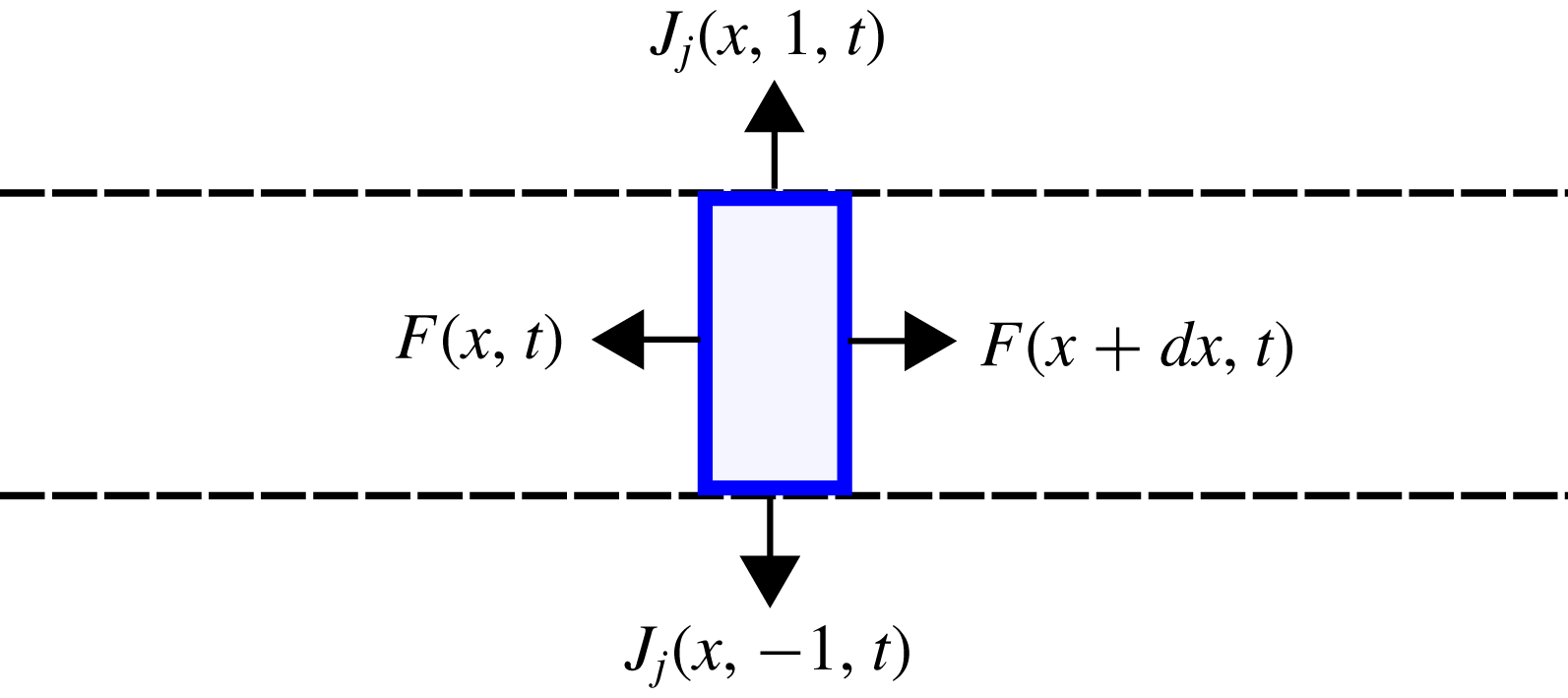
The effect of finite impedance can be explored by energy balance analysis of the control volume shown in figure 12. Specifically, we compare energy fluxes across sections of the inner region (
 $F$
) to fluxes to and from the interfaces (
 $J_{vs}$
). The inner flux is given by,
 $$\begin{eqnarray}F(x,t)=\int _{-1}^{1}J_{i}(x,y,t)\,\text{d}y,\end{eqnarray}$$
while energy flux at the upper and lower vortex sheets is given by,
 $$\begin{eqnarray}J_{vs}(x,t)=J_{j}(x,1,t)-J_{j}(x,-1,t),\end{eqnarray}$$
where
 $(J_{i},J_{j})$
are the components of
 $\boldsymbol{J}$
, as defined by (4.2).
Schematic depiction of energy balance analysis. Control volume shown in blue, vortex sheets indicated by the black dashed lines and energy fluxes by arrows.

The time-averaged energy conservation law for the control volume becomes,
 $$\begin{eqnarray}\frac{\unicode[STIX]{x2202}}{\unicode[STIX]{x2202}x}{\mathcal{F}}(x)=-{\mathcal{J}}_{j}(x),\end{eqnarray}$$
with
 $$\begin{eqnarray}{\mathcal{F}}(x)=\langle F(x,t)\rangle ,\quad {\mathcal{J}}_{j}(x)=\langle J_{vs}(x,t)\rangle .\end{eqnarray}$$
Leading-order approximations of energy fluxes in the inner region and at the interfaces are obtained by assuming hard- and soft-walled duct behaviour,
 $$\begin{eqnarray}\hat{p}(y)=A(\text{e}^{\unicode[STIX]{x1D709}_{in}y}\pm \text{e}^{-\unicode[STIX]{x1D709}_{in}y}),\end{eqnarray}$$
the plus and minus signs being associated with symmetric and antisymmetric modes, respectively. The time-averaged duct-like energy flux for the symmetric mode is,
 $$\begin{eqnarray}\displaystyle {\mathcal{F}}(x)=\langle F(x,t)\rangle & = & \displaystyle \int _{-1}^{1}\langle \,\boldsymbol{J}_{i}(y)\rangle \,\text{d}y\nonumber\\ \displaystyle & = & \displaystyle \frac{|A|^{2}}{\unicode[STIX]{x1D70C}_{in}}\frac{c}{c-U_{in}}\left(\frac{1}{c-U_{in}}+\frac{U_{in}}{a_{in}^{2}}\right)\int _{-1}^{1}\cos \left(\frac{n\unicode[STIX]{x03C0}}{2}y\right)^{2}\text{d}y\nonumber\\ \displaystyle & = & \displaystyle \frac{|A|^{2}}{\unicode[STIX]{x1D70C}_{in}}\frac{c}{c-U_{in}}\left(\frac{1}{c-U_{in}}+\frac{U_{in}}{a_{in}^{2}}\right),\end{eqnarray}$$
a similar result being obtained for the antisymmetric modes. The average net energy flux at the interface is given by,
 $$\begin{eqnarray}\displaystyle {\mathcal{J}}_{j}(x) & = & \displaystyle \langle J_{j}(x,1^{-},t)-J_{j}(x,-1^{+},t)\rangle \nonumber\\ \displaystyle & = & \displaystyle (\text{Re}(\hat{v}(1)\hat{p}^{+}(1))-\text{Re}(\hat{v}(-1)\hat{p}^{+}(-1)))\unicode[STIX]{x1D70C}_{in}\frac{c}{c-U_{in}}.\end{eqnarray}$$
For a duct mode, either
 $\hat{p}(\pm 1)=0$
(soft duct) or
 $\hat{v}(\pm 1)=0$
(hard duct), both of which lead to zero interface flux and thus to constant flux in the inner region. A first-order correction for the interface flux of modes departing from these behaviours is obtained by expanding the components
 $p^{\prime }$
and
 $v^{\prime }$
up to first order,
 $$\begin{eqnarray}\hat{p}=\hat{p}_{0}+\unicode[STIX]{x1D6FF}\hat{p},\quad \hat{v}=\hat{v}_{0}+\unicode[STIX]{x1D6FF}\hat{v},\end{eqnarray}$$
the constraint at the interface being,
 $$\begin{eqnarray}\hat{p}_{0}+\unicode[STIX]{x1D6FF}\hat{p}=(\hat{v}_{0}+\unicode[STIX]{x1D6FF}\hat{v}){\mathcal{Z}}_{VS}.\end{eqnarray}$$
For large
 ${\mathcal{Z}}_{VS}$
and
 $\hat{v}_{0}=0$
, the leading terms are,
 $$\begin{eqnarray}\unicode[STIX]{x1D6FF}\hat{p}=0,\quad \unicode[STIX]{x1D6FF}\hat{v}=\frac{\hat{p}_{0}}{{\mathcal{Z}}_{VS}},\end{eqnarray}$$
while for small
 ${\mathcal{Z}}_{VS}$
and
 $\hat{p}_{0}=0$
, we have,
 $$\begin{eqnarray}\unicode[STIX]{x1D6FF}\hat{p}=\hat{v}_{0}{\mathcal{Z}}_{VS},\quad \unicode[STIX]{x1D6FF}\hat{v}=0.\end{eqnarray}$$
Expressions for the interface energy flux under hard- and soft-walled duct approximations are obtained, respectively, by inserting (4.14) or (4.15) into (4.13) and (4.11),
 $$\begin{eqnarray}\displaystyle & \displaystyle {\mathcal{J}}_{j}^{h}=2|A|^{2}\frac{c}{c-U_{in}}\text{Re}({\mathcal{Z}}_{VS}^{-1}), & \displaystyle\end{eqnarray}$$
 $$\begin{eqnarray}\displaystyle & \displaystyle {\mathcal{J}}_{j}^{s}=2|A|^{2}\frac{|\unicode[STIX]{x1D709}_{in}|^{2}}{\unicode[STIX]{x1D70C}_{in}^{2}|\unicode[STIX]{x1D6FC}(c-U_{in})|^{2}}\frac{c}{c-U_{in}}\text{Re}({\mathcal{Z}}_{VS}). & \displaystyle\end{eqnarray}$$
If
 $|{\mathcal{J}}_{j}^{s,h}|\ll |{\mathcal{F}}|$
, a slowly varying amplitude,
 $A=A(x)$
, may be assumed. The
 $x$
-dependence of the amplitude is obtained by inserting (4.10) and (4.16) or (4.17) into (4.7), giving,
 $$\begin{eqnarray}\frac{\unicode[STIX]{x2202}|A(x)|^{2}}{\unicode[STIX]{x2202}x}=-\frac{{\mathcal{J}}^{s,h}}{{\mathcal{F}}}|A(x)|^{2},\end{eqnarray}$$
and thus
 $$\begin{eqnarray}|A(x)|=|A(0)|\text{e}^{-({\mathcal{J}}^{s,h}/2{\mathcal{F}})x}.\end{eqnarray}$$
This spatial dependence can be seen as a wavenumber correction,
 $$\begin{eqnarray}\unicode[STIX]{x0394}\unicode[STIX]{x1D6FC}_{i}=\frac{{\mathcal{J}}^{s,h}}{2{\mathcal{F}}},\end{eqnarray}$$
which scales with
 $\text{Re}(1/{\mathcal{Z}}_{VS})$
and
 $\text{Re}({\mathcal{Z}}_{VS})$
for soft- and hard-walled duct modes, respectively. Using (3.3) the correction for a hard-walled duct becomes,
 $$\begin{eqnarray}\unicode[STIX]{x0394}\unicode[STIX]{x1D6FC}_{i}=\frac{{\mathcal{J}}^{h}}{2{\mathcal{F}}}=\frac{a_{in}^{2}\unicode[STIX]{x1D70C}_{in}}{v_{group}}\text{Re}({\mathcal{Z}}_{VS}^{-1}).\end{eqnarray}$$
Convective stability/instability is thus associated with negative/positive values of
 $\text{Re}({\mathcal{Z}}_{VS})$
. An analogous result is found for soft-walled ducts. A similar relation between stability in ducts and the real part of the impedance has been described by Rienstra & Hirschberg (Reference Rienstra and Hirschberg2018).
4.3 Finite impedances in a compressible wake
We now explore a first-order approximation for finite impedance (4.20) in a Mach 0.9 wake. In order to isolate impedance effects, root loci are mapped as a function of
 $\unicode[STIX]{x1D70C}_{r}$
: with
 $\unicode[STIX]{x1D714}$
and
 $T_{r}$
maintained constant, the propagative/evanescent characteristics of the soft-walled duct modes remain unaltered. The spatial eigenspectrum for
 $\unicode[STIX]{x1D70C}_{r}=1$
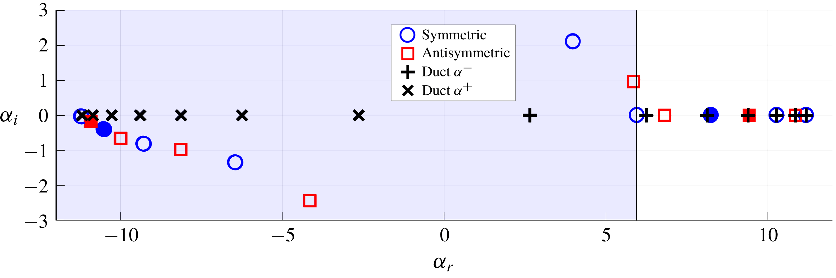
is shown in figure 13. Modes in the left and right half-planes are, respectively, upstream and downstream travelling. All subsonic modes are constrained to the real
 $\unicode[STIX]{x1D6FC}$
axis, and closely match the duct modes. Supersonic modes are all damped (i.e. they decay in the direction of generalised group velocity (Bers Reference Bers1975)), and resemble attenuated duct modes.
Roots of (2.11) for
 $V_{ref}=0$
,
 $M=0.9$
,
 $\unicode[STIX]{x1D70C}_{in,out}=1$
and
 $\unicode[STIX]{x1D714}=4\unicode[STIX]{x03C0}$
. Blue and red markers indicate symmetric and antisymmetric modes, respectively, solid circles indicate the modes considered in figures 14 and 15. Hard- and soft-walled duct roots are indicated by ‘
 $\times$
’ and ‘
 $+$
’, respectively. The blue region indicates supersonic phase velocity with respect to the outer flow.

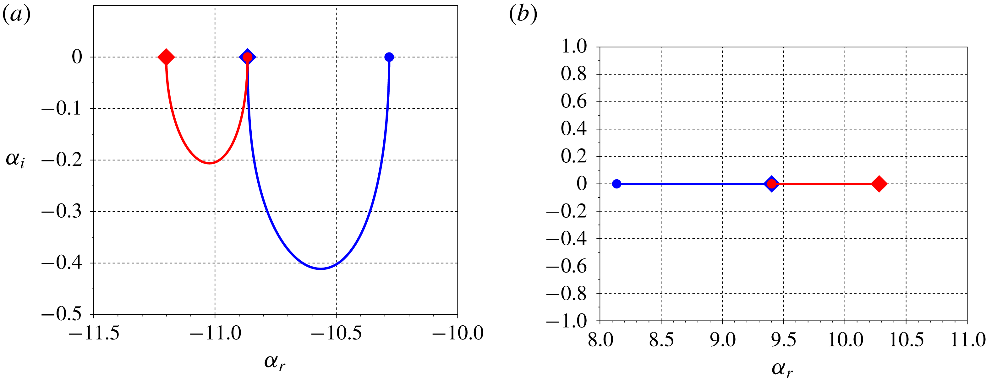
Figure 14 maps loci of the modes indicated by solid markers in figure 13 as
 $\unicode[STIX]{x1D70C}_{r}$
is varied. Supersonic modes make an excursion into the complex
 $\unicode[STIX]{x1D6FC}$
plane, while subsonic modes are restricted to the real axis due to total internal reflection, as predicted by (4.2). Figure 15 compares
 $\unicode[STIX]{x1D6FC}_{i}$
with the predictions of (4.20), which accurately captures the spatial amplitude variation of these modes for most impedance values, failing only when the DVS transitions between soft- and hard-walled duct behaviours. The results illustrates how energy fluxes through the vortex sheets constitute the stabilisation mechanism of the acoustic modes.
Loci, as a function of
 $\unicode[STIX]{x1D70C}_{r}$
, of upstream- (a) and downstream- (b) travelling modes, indicated in the left and right half-planes of figure 13. Upstream-travelling modes move in to the complex
 $\unicode[STIX]{x1D6FC}$
plane, while downstream-travelling modes remain on the real axis due to total reflection. Limits of hard- (
 $\unicode[STIX]{x1D70C}_{r}=\infty$
) and soft-duct (
 $\unicode[STIX]{x1D70C}_{r}=0$
) behaviour are indicated, respectively, by diamonds and circles. Red and blue lines represent antisymmetric and symmetric modes, respectively.


4.4 Finite impedances in compressible jets
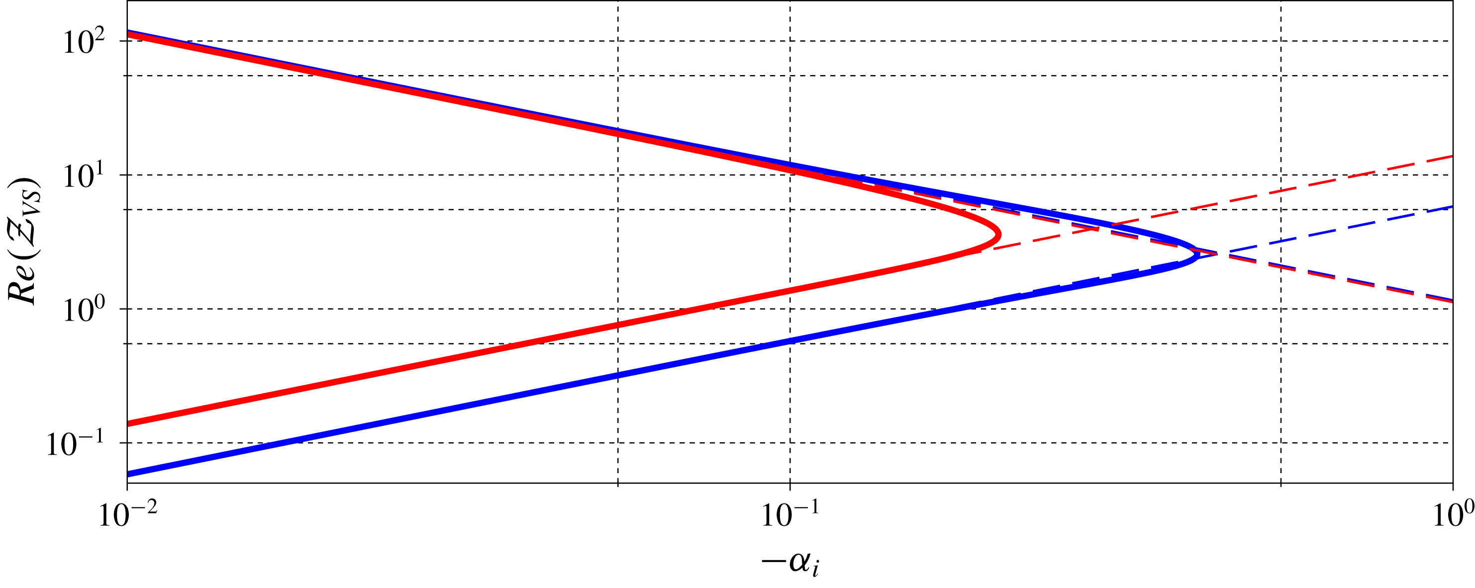
We now consider a regime in which the real part of the impedance becomes negative. Inspection of (3.7) shows that the term
 $\unicode[STIX]{x1D70C}_{out}(c-U_{out})^{2}$
is always positive and real,
 $\text{i}\unicode[STIX]{x1D709}_{out}$
is imaginary or positive real and so only the term
 $\unicode[STIX]{x1D6FC}/(c-U_{in})$
may be either positive or negative. Expanding this term with (3.2), we obtain,
 $$\begin{eqnarray}{\displaystyle \frac{\unicode[STIX]{x1D6FC}}{c-U_{in}}}={\displaystyle \frac{\unicode[STIX]{x1D6FC}^{2}(U_{in}^{2}/a^{2}-1)}{\unicode[STIX]{x1D714}\left(-1\pm U_{in}/a\sqrt{1+{\displaystyle \frac{(n\unicode[STIX]{x03C0}/2)^{2}(U_{in}^{2}-a^{2})}{\unicode[STIX]{x1D714}^{2}}}}\right)}},\end{eqnarray}$$
where
 $\pm$
corresponds to the
 $\unicode[STIX]{x1D6FC}^{+}$
and
 $\unicode[STIX]{x1D6FC}^{-}$
modes. For a left-pointing supersonic jet (
 $U_{in}<-a$
), the ratio
 $\unicode[STIX]{x1D6FC}/(c-U_{in})$
is always positive for
 $\unicode[STIX]{x1D6FC}^{-}$
modes and negative for
 $\unicode[STIX]{x1D6FC}^{+}$
. If they have supersonic phase speeds, the
 $\unicode[STIX]{x1D6FC}^{-}$
and
 $\unicode[STIX]{x1D6FC}^{+}$
modes become, respectively, stable and unstable, the number of supersonic modes increasing with Mach number.
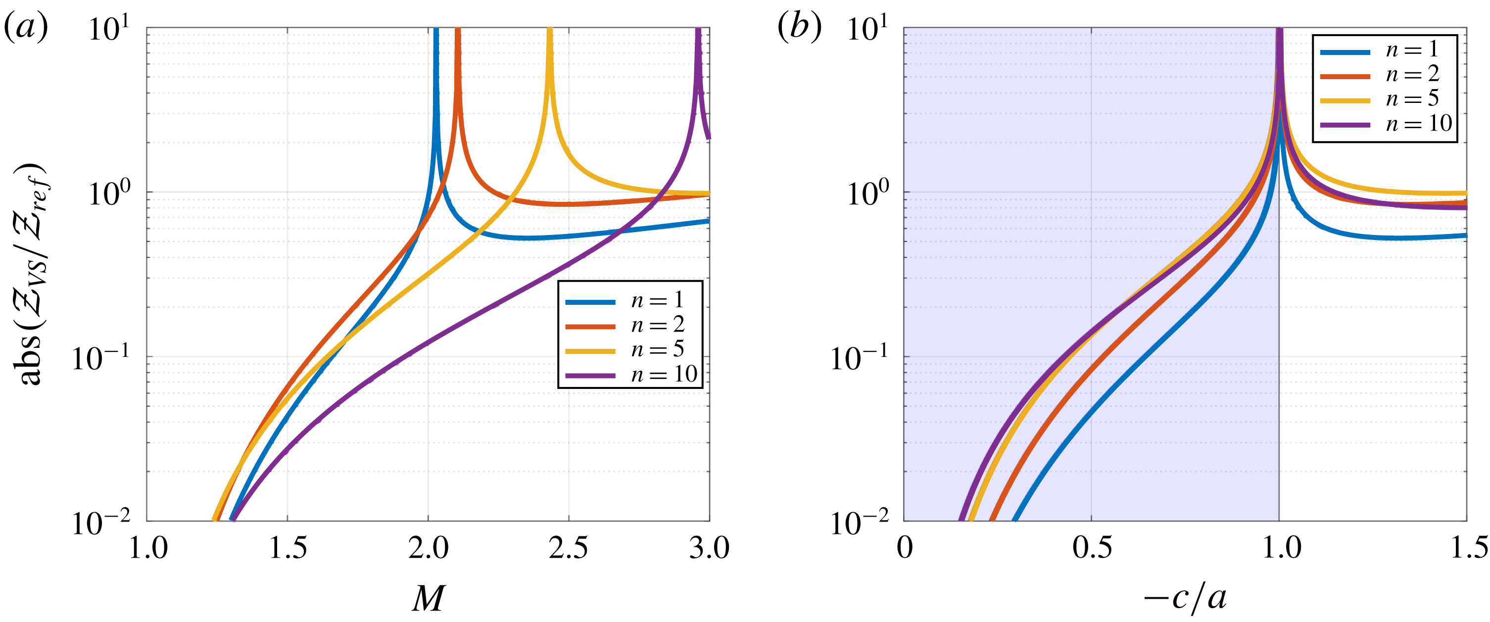
Figure 16 shows the impedances associated with
 $\unicode[STIX]{x1D6FC}^{+}$
duct-mode ansätze for a jet, as a function of Mach number. The impedance presents spikes whose locations collapse when scaled using duct-mode phase speeds. The impedance spikes are related to transition between sub- and super-sonic phase speeds: at the sonic limit,
 $\unicode[STIX]{x1D709}_{out}\rightarrow 0$
, and thus,
 ${\mathcal{Z}}_{VS}\rightarrow \infty$
. The flow transitions from soft- to hard-walled duct behaviour.
Absolute values of impedance for
 $\unicode[STIX]{x1D6FC}^{+}$
duct modes as a function of Mach number (a) and of duct-mode phase speed (b). Impedance peaks, found at different
 $M$
for each harmonic, occur when the phase speed of the mode is sonic. Results are for
 $\unicode[STIX]{x1D714}=\unicode[STIX]{x03C0}$
, with the blue region indicating subsonic phase speeds.

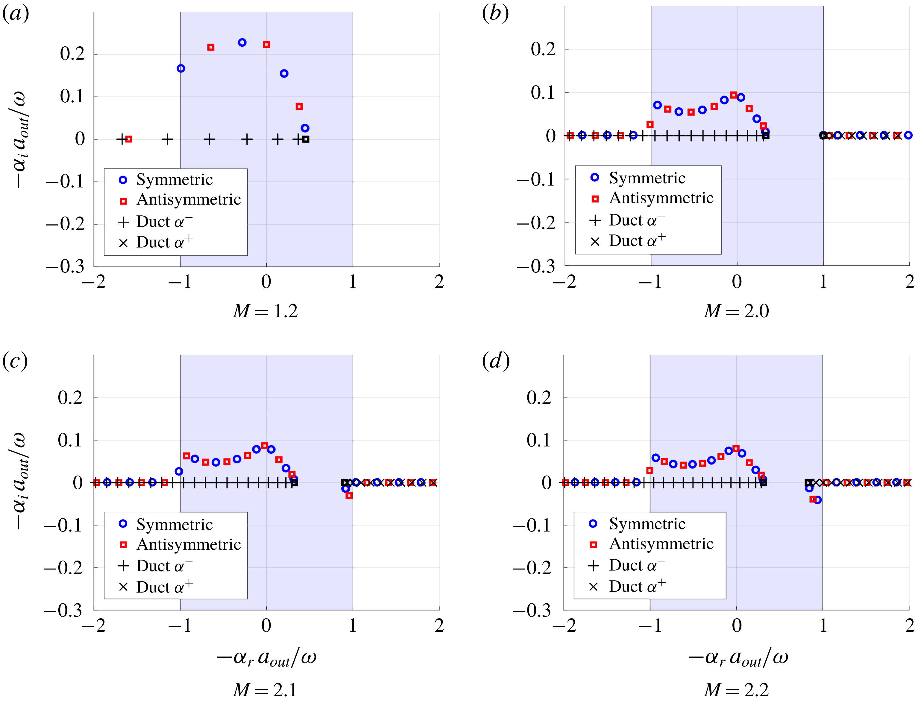
Figure 17 compares the DVS modes of a supersonic jet to
 $\unicode[STIX]{x1D6FC}^{-}$
and
 $\unicode[STIX]{x1D6FC}^{+}$
duct modes, illustrating a correspondence between jet and duct behaviour. As predicted, waves corresponding to
 $\unicode[STIX]{x1D6FC}^{-}$
(respectively
 $\unicode[STIX]{x1D6FC}^{+}$
) duct modes exhibit spatial decay (respectively growth). The transition from soft- to hard-walled behaviour is seen in figure 18. Supersonic
 $\unicode[STIX]{x1D6FC}^{+}$
modes correspond to the unstable supersonic modes of Tam & Hu (Reference Tam and Hu1989b
): figure 17 corresponds to the transition between the subsonic and supersonic scenarios discussed in their work (cf. figures 11 and 10, respectively, in Tam & Hu Reference Tam and Hu1989b
). We thus see that the instability mechanism identified by Tam & Hu (Reference Tam and Hu1989b
) is underpinned by interaction of acoustic modes with the vortex sheet, and an associated influx of energy if the conditions discussed above are satisfied.
Instability of supersonic
 $\unicode[STIX]{x1D6FC}^{+}$
and stability of supersonic
 $\unicode[STIX]{x1D6FC}^{-}$
modes for a left-pointing jet. Results are plotted in terms of
 $-\unicode[STIX]{x1D6FC}$
. All subsonic modes are neutrally stable, all supersonic modes being either stable (
 $-\unicode[STIX]{x1D6FC}_{i}>0$
) or unstable (
 $-\unicode[STIX]{x1D6FC}_{i}<0$
). Coloured markers indicate DVS modes, black markers indicated duct modes, with the
 $n=0$
mode identified by a square marker: this mode is not present in the soft-walled limit, appearing only at the transition to hard-walled behaviour. The blue region indicates supersonic phase speeds with respect to the outer region. Mach numbers 1.2, 2.0, 2.1, 2.2 from left to right, top to bottom. The plot is for constant Helmholtz numbers,
 $\unicode[STIX]{x1D714}=\unicode[STIX]{x03C0}$
, and
 $\unicode[STIX]{x1D70C}_{r}=T_{r}=1$
.

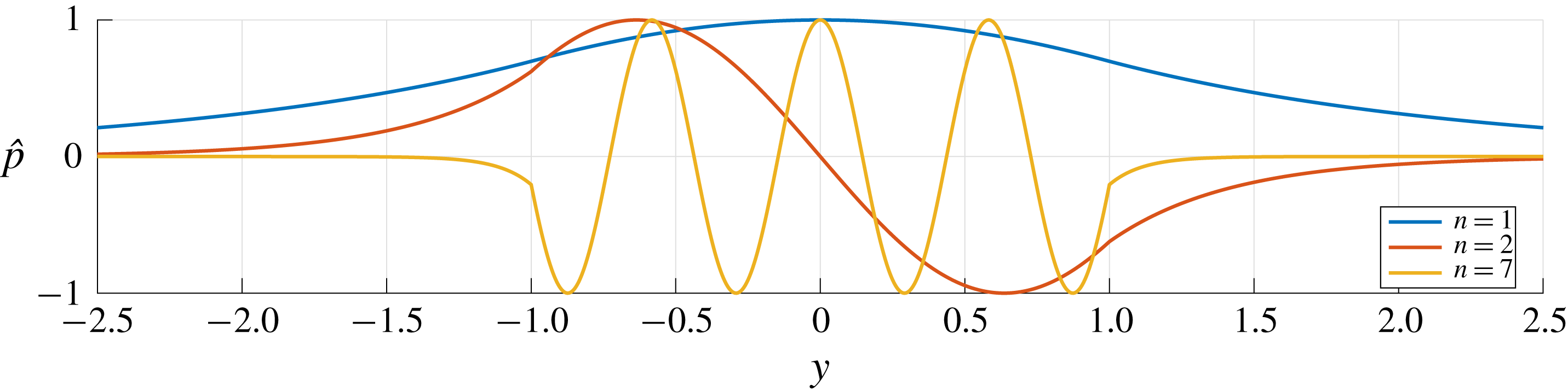
Pressure support for the first, second and seventh
 $\unicode[STIX]{x1D6FC}^{+}$
duct-like modes in a
 $M=2.0$
jet. Lower harmonics, which have near-sonic phase velocities with respect to the outer flow, resemble hard-walled duct modes; a transition to soft-duct behaviour is observed as the harmonic number increases. Results are for
 $V_{ref}=1$
and
 $\unicode[STIX]{x1D714}=\unicode[STIX]{x03C0}$
.

4.5 Summary
In this section we have shown how vortex-sheet impedance is a key parameter for the dynamics of acoustic modes. Analysis of the acoustic energy budget shows how outflux (respectively influx) of acoustic energy associated with a real, positive (respectively negative) vortex-sheet impedance is the key to stabilisation (respectively destabilisation). We see how this can explain the stabilisation of acoustic modes in a compressible wake, and, perhaps more importantly, the appearance of unstable modes in supersonic jets (Tam & Hu Reference Tam and Hu1989b ).
In the next section impulse responses are computed. The goal is twofold: by constructing the DVS impulse response we confirm the statement made in § 3.3 regarding the stabilisation of jets, but not of wakes, that occurs on account of compressibility effects. And by constructing wavepackets for finite-thickness shear layers we show that the transition to absolute instability associated with saddles formed by KH and upstream-travelling acoustic modes, presented in § 3.2, also exists when finite-thickness shear layers are considered.
5 Impulse response
5.1 Impulse response of DVS
The long-time impulse response is underpinned by the dominant saddle point of the dispersion relation (Huerre & Monkewitz Reference Huerre and Monkewitz1985). The saddle points are identified by a zero generalised group velocity
 $$\begin{eqnarray}\frac{\unicode[STIX]{x2202}\unicode[STIX]{x1D714}}{\unicode[STIX]{x2202}\unicode[STIX]{x1D6FC}}=\left.-\frac{\unicode[STIX]{x2202}D_{dvs}}{\unicode[STIX]{x2202}\unicode[STIX]{x1D6FC}}\right/\frac{\unicode[STIX]{x2202}D_{dvs}}{\unicode[STIX]{x2202}\unicode[STIX]{x1D714}}=0,\end{eqnarray}$$
with
 $D_{dvs}$
given by (2.11). The ill-posed nature of the vortex-sheet model has been evoked in § 3.2: vortex sheets possess unbounded growth rates with increasing
 $\unicode[STIX]{x1D714}$
; the inclusion of a small shear-layer thickness regularises the problem. The absolute stability analysis thus amounts to a search for modes scaling with jet or wake width in the limit of small shear-layer thickness, as in Yu & Monkewitz (Reference Yu and Monkewitz1990). Because of this, we choose to refer to the DVS wavepacket (impulse response) as a pseudo-wavepacket, calculated by mapping the dispersion-relation saddle points for each
 $V_{ref}$
. The wavepackets so obtained can be used to infer the impulse response of any of the DVS base flows by a simple change of reference frame: for any
 $V_{ref}$
the maximum growth rate for a space–time ray,
 $x/t=v^{\ast }$
, is obtained from the saddle point with maximum
 $\unicode[STIX]{x1D714}_{0,i}$
, of a flow with
 $V_{ref}^{\ast }=V_{ref}+v^{\ast }$
. Details of the computation are provided in § B.1.
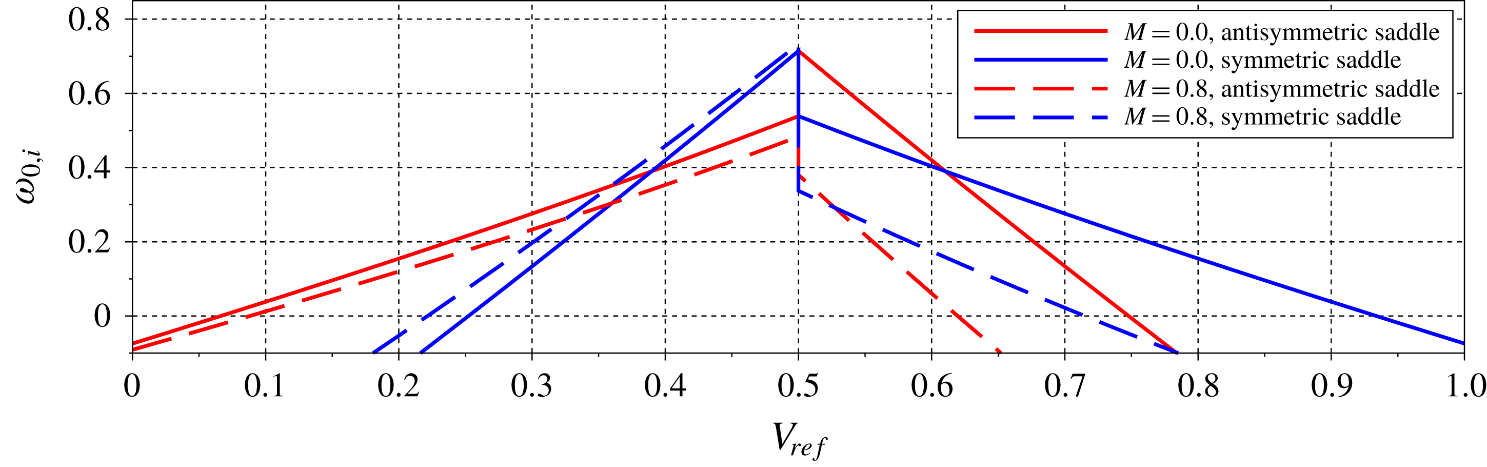
The pseudo-wavepackets, whose growth rates are shown in figure 19, present two distinct regimes: the jet-like regime (
 $V_{ref}>0.5$
) is dominated by symmetric modes, and compressibility has a strong stabilising effect, while the wake-like regime (
 $V_{ref}<0.5$
) is dominated by antisymmetric modes with small sensitivity to compressibility. The large stabilisation effect in the jet regime is attributed to the presence of total internal reflection, as shown in figure 10.
Growth rates of pseudo-wavepackets of the DVS flow for
 $T_{r}=1$
.

5.2 Impulse response of finite shear-layer flows
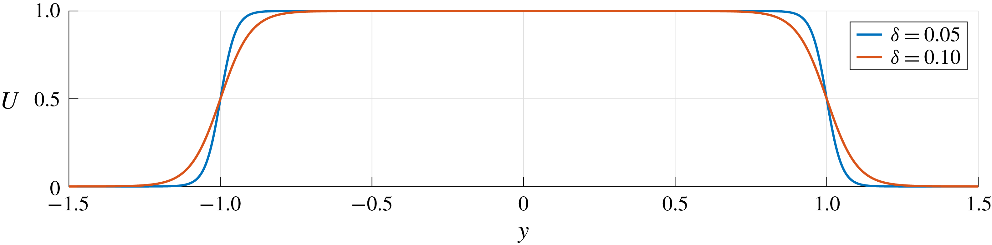
We extend the foregoing results to base flows with finite-thickness shear layers. We consider a profile modelled as,
 $$\begin{eqnarray}U(y)=(U_{in}-U_{out})\left(\frac{\tanh \left({\displaystyle \frac{y+1}{\unicode[STIX]{x1D6FF}}}\right)+\tanh \left(-{\displaystyle \frac{y-1}{\unicode[STIX]{x1D6FF}}}\right)}{2\tanh \left({\displaystyle \frac{1}{\unicode[STIX]{x1D6FF}}}\right)}\right)+U_{out},\end{eqnarray}$$
where
 $\unicode[STIX]{x1D6FF}$
controls the shear-layer thickness, as illustrated in figure 20. The DVS model is recovered when
 $\unicode[STIX]{x1D6FF}\rightarrow 0$
. We restrict our study to the incompressible regime. The modes were obtained by a discretisation of the Rayleigh equation using Gauss–Lobatto points. A pseudo-spectral code based on Chebyshev polynomials was used to obtain the derivatives at each point and standard generalised eigenvalue routines were used, as in Ormonde et al. (Reference Ormonde, Cavalieri, da Silva and Avelar2018). Details of the procedures used can be found in § B.2.
Illustration of a finite shear-layer jet obtained with (5.2).

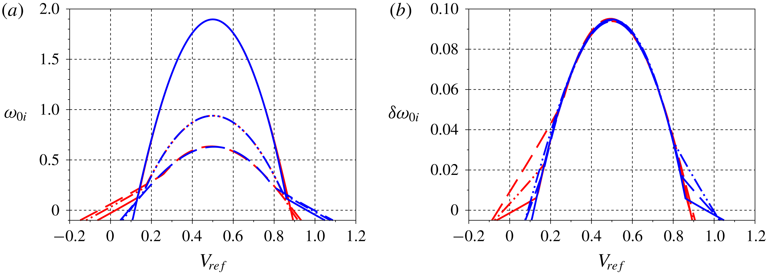
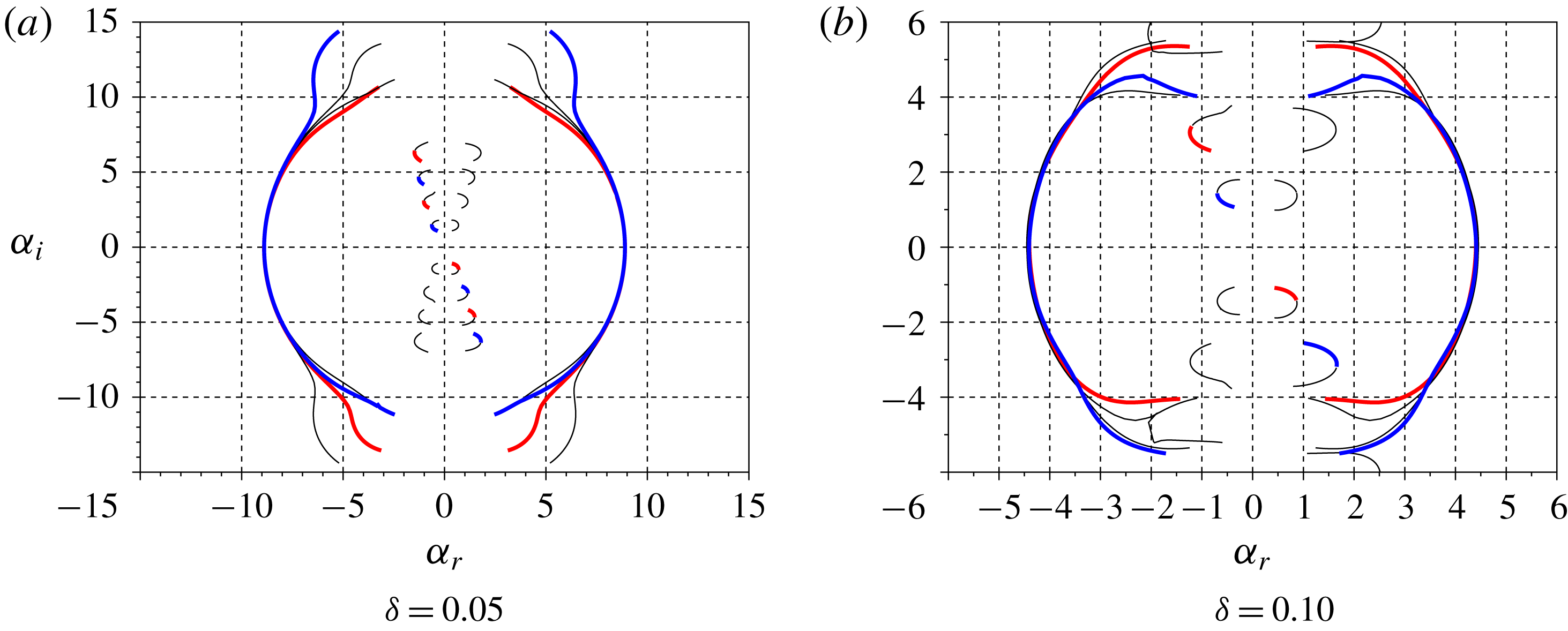
Figure 21 shows wavepacket growth rates for different values of
 $\unicode[STIX]{x1D6FF}$
. For jets and wakes with small backflow, the instability scales with the distance between the vortex sheets, corresponding to the DVS saddle points studied in the previous sections, slightly altered by shear-layer thickness. We refer to this saddle point as the column saddle, following Lesshafft & Huerre (Reference Lesshafft and Huerre2007); it corresponds to mode II in Jendoubi & Strykowski (Reference Jendoubi and Strykowski1994). For large reverse flows (
 $0.2<V_{ref}<0.8$
) the instability scales with
 $\unicode[STIX]{x1D6FF}^{-1}$
and we refer to it as the shear-layer saddle, again following Lesshafft & Huerre (Reference Lesshafft and Huerre2007); it corresponding to mode I of Jendoubi & Strykowski (Reference Jendoubi and Strykowski1994). This saddle point is characterised by large values of
 $|\unicode[STIX]{x1D6FC}_{r}|$
, suggesting negligible interaction between the vortex sheets; it thus corresponds to the saddle point studied by Huerre & Monkewitz (Reference Huerre and Monkewitz1985).
Although the shear-layer saddle point dominates most of the wavepacket, it is the column saddles that, due to backflow, first exhibit temporal growth, showing how acoustic modes are associated with the primary destabilisation mechanism of wakes and jets with finite-thickness shear layers. We also see that wakes are more sensitive to shear-layer thickness than jets, becoming unstable even in the absence of reverse flow due to finite-thickness shear layers, while jets remain marginally stable.
A more complete investigation of the effects of shear-layer thickness effects on compressible jets can be found in Tam & Hu (Reference Tam and Hu1989a
), where it is shown that subsonic modes may become unstable due to finite shear-layer thickness; and in Parras & Le Dizès (Reference Parras and Le Dizès2010), where asymptotic expansions show that the presence of critical points (where
 $c=U(y)$
) are related to the instability of the acoustic modes.
Wavepacket growth rates for
 $\unicode[STIX]{x1D6FF}=0.05,0.10$
and 0.20 (solid, dashed and dotted lines, respectively). Blue and red lines correspond to symmetric and antisymmetric modes, respectively. (a) Growth rates based on shear-layer separation; (b) growth rates rescaled using the shear-layer thickness
 $\unicode[STIX]{x1D6FF}$
.

6 Conclusion
Discrete modes of an acoustic nature have been identified in both compressible and incompressible double vortex-sheet (DVS) flow models, which we have configured in order to describe the behaviour of both jets and wakes. In the incompressible regime, they reduce to evanescent, exponentially decaying disturbances, which satisfy the Laplace equation. An analogy between these guided modes and acoustic modes found in ducts has been formulated, and it requires one of two a priori conditions for its validity: (i) limiting values of vortex-sheet impedance, which are required to be either much larger or much smaller than a reference value; or, (ii) the presence of total reflection, with evanescent-wave dynamics in the outer flow. Duct-like modes are found in both jets and wakes over an extensive parameter space, generalising the analysis of Towne et al. (Reference Towne, Cavalieri, Jordan, Colonius, Schmidt, Jaunet and Brès2017) for a broader class of flows; and, in particular, in the incompressible limit, where acoustic waves become evanescent pressure modes.
We show how upstream-travelling acoustic modes are central for a complete understanding of absolute instability. Specifically, deterioration of their duct-like behaviour appears as a necessary condition for the onset of instability. When the acoustic modes are duct-like, jets and wakes behave as waveguides, and upstream-travelling modes have negligible interaction with KH modes. A departure from duct-like behaviour enables interaction between acoustic and KH modes, a neutral saddle point eventually forming between the two and marking the onset of absolute instability. This scenario was verified to hold in both incompressible and compressible regimes.
The mechanisms we discuss are similar in some respects to those discussed by Healey (Reference Healey2009), where confinement effects were shown to lead to absolute instability due to the action of acoustic modes. Healey’s acoustic modes scale with the distance between confining walls, which are imposed. In our work they scale with the distance between vortex sheets, and the ‘wall’ behaviour is an intrinsic part of the flow dynamics.
The phenomena we consider are also relevant for global instabilities, as for slowly diverging base flows, global modes may be built using the Wentzel–Kramers–Brillouin–Jeffrey method (Monkewitz et al. Reference Monkewitz, Huerre and Chomaz1993; Siconolfi et al. Reference Siconolfi, Citro, Giannetti, Camarri and Luchini2017), which shows the global instability to arise on account of local pockets of absolute instability. Investigating of these modes in non-parallel systems would thus appear worthwhile, as the global stability of a given system might be modified/controlled via an appropriate manipulation of the acoustic mode.
The departure from duct-like behaviour was explored via an energy balance analysis, derived in § 4. Energy fluxes through the vortex sheets are associated with spatial growth or decay of the acoustic-mode amplitude. Energy outflow and inflow were shown to underpin, respectively, the stabilisation and destabilisation of acoustic modes, and it was shown how this behaviour is associated with the unstable supersonic modes identified by Tam & Hu (Reference Tam and Hu1989b ). First-order corrections were derived in order to described acoustic-mode amplitude variations close to the duct-limit conditions.
Impulse responses of jets and wakes with vanishing and finite-thickness shear layers were computed, supporting previous results and showing that the main conclusions of our analysis also hold for flows with finite-thickness shear layers, and are not an artefact of the vortex-sheet model. The saddle points associated with finite-thickness shear-layer flows are most relevant for absolute instability when strong reverse flow exists. For jets and wakes with little or no reverse flow, the absolute/convective stability behaviour is found to be dominated by interaction between KH and the upstream-travelling, acoustic modes we consider.
The analysis opens up new possibilities for the study of global instability in free-shear flows. Clarification of the role played by acoustic modes has permitted a unified explanation of known, but previous unconnected, trends found in the literature: (i) transition from convective to absolute instability due to backflow, wake cooling (Monkewitz Reference Monkewitz1988) and jet heating (Monkewitz & Sohn Reference Monkewitz and Sohn1988); (ii) the differing symmetries of unstable wakes and jets (Yu & Monkewitz Reference Yu and Monkewitz1990); (iii) acoustic wave trapping (Schmidt et al. Reference Schmidt, Towne, Colonius, Cavalieri, Jordan and Brès2017; Towne et al. Reference Towne, Cavalieri, Jordan, Colonius, Schmidt, Jaunet and Brès2017); and, (iv) the unstable supersonic jet modes of Tam & Hu (Reference Tam and Hu1989b ).
Perhaps more interestingly, the fact that acoustic phenomena are central in the destabilisation of wakes (leading to the well-known von Kármán vortex street in the saturated limit) and hot jets, suggests the possibility of novel approaches for flow control. Instead of targeting the classical KH instability, one may consider modifying the behaviour of a flow by targeting the modes studied here.
Acknowledgements
A.V.G.C. acknowledges financial support by CNPq (grant number 310523/2017-6). E.M. acknowledges financial support from CAPES (grant number 88881.190271/2018-01).
Appendix A. Review of duct acoustics
Given a duct containing a uniform, two-dimensional flow of velocity
 $U$
, the linearised Euler equations can be simplified, leading to the convected wave equation,
 $$\begin{eqnarray}\left({\displaystyle \frac{\unicode[STIX]{x2202}}{\unicode[STIX]{x2202}t}}+U{\displaystyle \frac{\unicode[STIX]{x2202}}{\unicode[STIX]{x2202}x}}\right)^{2}p^{\prime }-a^{2}\left({\displaystyle \frac{\unicode[STIX]{x2202}^{2}}{\unicode[STIX]{x2202}x^{2}}}+{\displaystyle \frac{\unicode[STIX]{x2202}^{2}}{\unicode[STIX]{x2202}y^{2}}}\right)p^{\prime }=0,\end{eqnarray}$$
where
 $t$
denotes time,
 $(x,y)$
streamwise and wall-normal Cartesian coordinates,
 $p^{\prime }$
the pressure fluctuations and
 $a$
the speed of sound. We assume hard walls at
 $y=\pm 1$
, and associated boundary conditions
 $\unicode[STIX]{x2202}p^{\prime }/\unicode[STIX]{x2202}y(\pm 1)=0$
.
Using the ansatz
 $$\begin{eqnarray}p^{\prime }(x,y,t)=\text{e}^{\text{i}(\unicode[STIX]{x1D6FC}x-\unicode[STIX]{x1D714}t)}(A\sin (\unicode[STIX]{x1D6FD}y)+B\cos (\unicode[STIX]{x1D6FD}y)),\end{eqnarray}$$
where
 $\unicode[STIX]{x1D6FC}$
and
 $\unicode[STIX]{x1D6FD}$
are streamwise,
 $x$
and wall-normal,
 $y$
, wavenumbers, and
 $\unicode[STIX]{x1D714}$
is frequency, the dispersion relation,
 $$\begin{eqnarray}(\unicode[STIX]{x1D714}-U\unicode[STIX]{x1D6FC})^{2}=a^{2}(\unicode[STIX]{x1D6FC}^{2}+\unicode[STIX]{x1D6FD}^{2}),\end{eqnarray}$$
is obtained. Boundary conditions enforce
 $\unicode[STIX]{x1D6FD}=\unicode[STIX]{x03C0}n/2$
, where
 $n$
is an integer harmonic number. Odd values of
 $n$
imply
 $B=0$
, leading to antisymmetric pressure distributions, while even values imply
 $A=0$
, and symmetric pressure distributions. Solving for the horizontal phase speed,
 $c=\unicode[STIX]{x1D714}/\unicode[STIX]{x1D6FC}$
, as a function of
 $\unicode[STIX]{x1D6FC}$
and
 $\unicode[STIX]{x1D6FD}$
, leads to modes corresponding to a temporal stability analysis, given by,
 $$\begin{eqnarray}c=U\pm a\sqrt{1+\frac{\unicode[STIX]{x1D6FD}^{2}}{\unicode[STIX]{x1D6FC}^{2}}},\end{eqnarray}$$
and with group velocity,
 $$\begin{eqnarray}v_{group}={\displaystyle \frac{\unicode[STIX]{x2202}\unicode[STIX]{x1D714}}{\unicode[STIX]{x2202}\unicode[STIX]{x1D6FC}}}=U+\frac{a}{(c-U)}a.\end{eqnarray}$$
For
 $U=0$
, the roots of (A 4) correspond to waves travelling to the right (plus sign) and to the left (minus sign). For non-zero
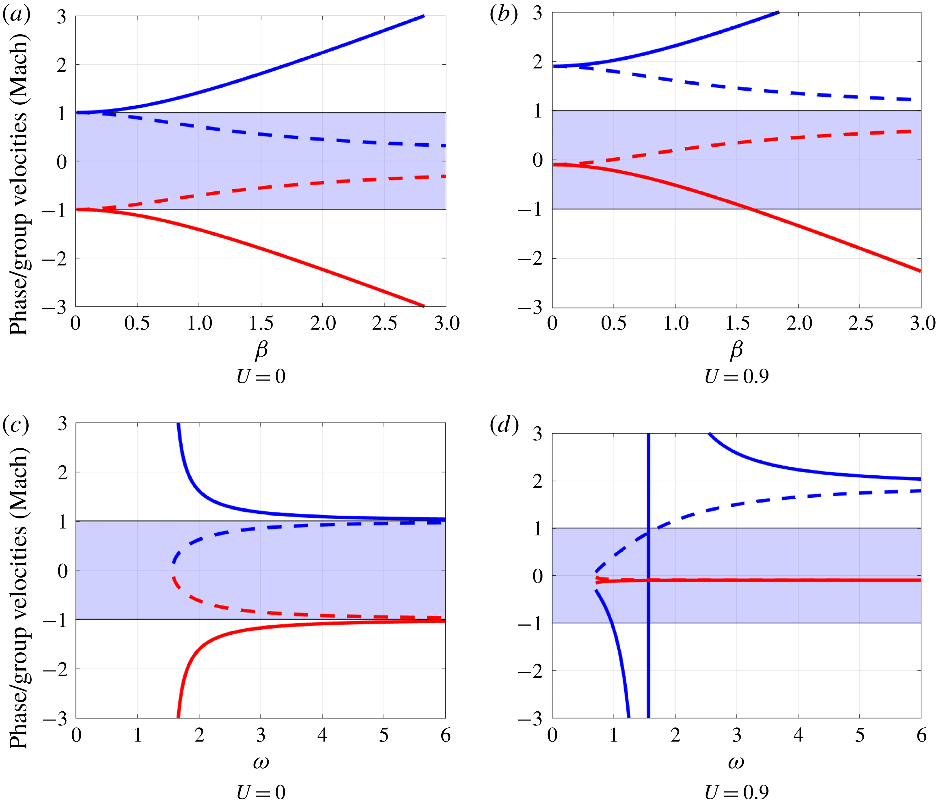
 $U$
the modes are convected by the mean flow, as illustrated in figure 22(a,b), where the phase velocity for a given
 $\unicode[STIX]{x1D6FC}$
and
 $\unicode[STIX]{x1D6FD}$
is shown. We note that for
 $U=0$
, modes have phase and group velocities of the same sign, whereas for
 $U=0.9$
in some cases we have a mode with negative phase speed and positive group velocity. Solving for
 $\unicode[STIX]{x1D6FC}$
, assuming fixed
 $\unicode[STIX]{x1D714}$
and
 $\unicode[STIX]{x1D6FD}$
,
 $$\begin{eqnarray}\unicode[STIX]{x1D6FC}=\frac{-U\unicode[STIX]{x1D714}\pm a\sqrt{\unicode[STIX]{x1D714}^{2}-(n\unicode[STIX]{x03C0}/2)^{2}(a^{2}-U^{2})}}{a^{2}-U^{2}},\end{eqnarray}$$
giving modes that would be consistent with a spatial stability analysis.
Behaviour of phase (solid) and group (dashed) velocities for the positive (red) and negative (blue) signs for propagative modes. Shaded regions indicate the subsonic velocities in the laboratory reference frame. For (a,b)
 $a=1$
,
 $\unicode[STIX]{x1D714}=1$
and
 $\unicode[STIX]{x1D6FC}(\unicode[STIX]{x1D714},\unicode[STIX]{x1D6FD})$
, while for (c,d)
 $a=1$
and
 $\unicode[STIX]{x1D6FD}=\unicode[STIX]{x03C0}/2$
were used, with
 $\unicode[STIX]{x1D714}(\unicode[STIX]{x1D6FC},\unicode[STIX]{x1D6FD})$
. The interdependency of
 $\unicode[STIX]{x1D6FC},\unicode[STIX]{x1D6FD},\unicode[STIX]{x1D714}$
are given by (A 3). Note that the boundary conditions limit the allowable values of
 $\unicode[STIX]{x1D6FD}$
to multiples of
 $\unicode[STIX]{x03C0}/2$
, nevertheless we keep all values of
 $\unicode[STIX]{x1D6FD}$
for a clearer visualisation of the trends.

Different scenarios emerge for real or complex
 $\unicode[STIX]{x1D6FC}$
. If
 $\unicode[STIX]{x1D6FC}$
is a purely real number it represents propagative modes, whose amplitudes are constant along the duct. They are found for,
 $$\begin{eqnarray}\unicode[STIX]{x1D714}^{2}>(n\unicode[STIX]{x03C0}/2)^{2}(a^{2}-U^{2}).\end{eqnarray}$$
At lower frequencies,
 $\unicode[STIX]{x1D6FC}$
has a non-zero imaginary part and the modes are evanescent, presenting exponential spatial decay in amplitude. For
 $U<a$
, the threshold between evanescent and propagative modes is given by the cut-on frequency,
 $$\begin{eqnarray}\unicode[STIX]{x1D714}_{cut\;on}=n\frac{\unicode[STIX]{x03C0}}{2}\sqrt{a^{2}-U^{2}},\end{eqnarray}$$
while for
 $U>a$
(supersonic flows) all acoustic modes are propagative and downstream travelling. Only evanescent modes are present in the incompressible limit (
 $a\rightarrow \infty$
).
Figure 22(c,d) shows phase and group velocities for a fixed
 $\unicode[STIX]{x1D6FD}=\unicode[STIX]{x03C0}/2$
(first harmonic), showing that in the presence of a mean flow and for frequencies slightly above the cut-on value, modes with both signs can have subsonic phase speeds. These are modes that are evanescent for
 $U=0$
but become propagative when flow is present, or equivalently, when the observer’s frame of reference changes (Rienstra & Hirschberg Reference Rienstra and Hirschberg2018).
Ducts with acoustically soft, or pressure release, walls have as boundary conditions,
 $p(\pm 1)=0$
. Modes in these ducts share the same properties and dispersion relation as the hard duct discussed above, differing in that the plane-wave mode (
 $n=0$
) only satisfies the boundary conditions for the hard-wall case, and in that modes have opposite symmetries in soft and hard ducts: odd modes (
 $n=1,3,5,\ldots$
) are antisymmetric and symmetric for hard and soft ducts, respectively, and the opposite being true for even modes (
 $n=2,4,6,\ldots$
).
Appendix B. Impulse response
B.1 DVS pseudo-wavepackets
Approximate DVS saddles were found by tracing root loci with increasing
 $\unicode[STIX]{x1D714}_{r}$
for different values of
 $\unicode[STIX]{x1D714}_{i}$
. Results were then refined by numerically solving
 $$\begin{eqnarray}D_{dvs}(\unicode[STIX]{x1D6FC},\unicode[STIX]{x1D714})=0,\quad \text{and}\quad \frac{\unicode[STIX]{x2202}\unicode[STIX]{x1D714}}{\unicode[STIX]{x2202}\unicode[STIX]{x1D6FC}}=\left.\frac{\unicode[STIX]{x2202}D_{dvs}}{\unicode[STIX]{x2202}\unicode[STIX]{x1D6FC}}\right/\frac{\unicode[STIX]{x2202}D_{dvs}}{\unicode[STIX]{x2202}\unicode[STIX]{x1D714}}=0,\end{eqnarray}$$
where
 $D_{dvs}$
is the dispersion relation of the DVS. The saddles loci with
 $V_{ref}$
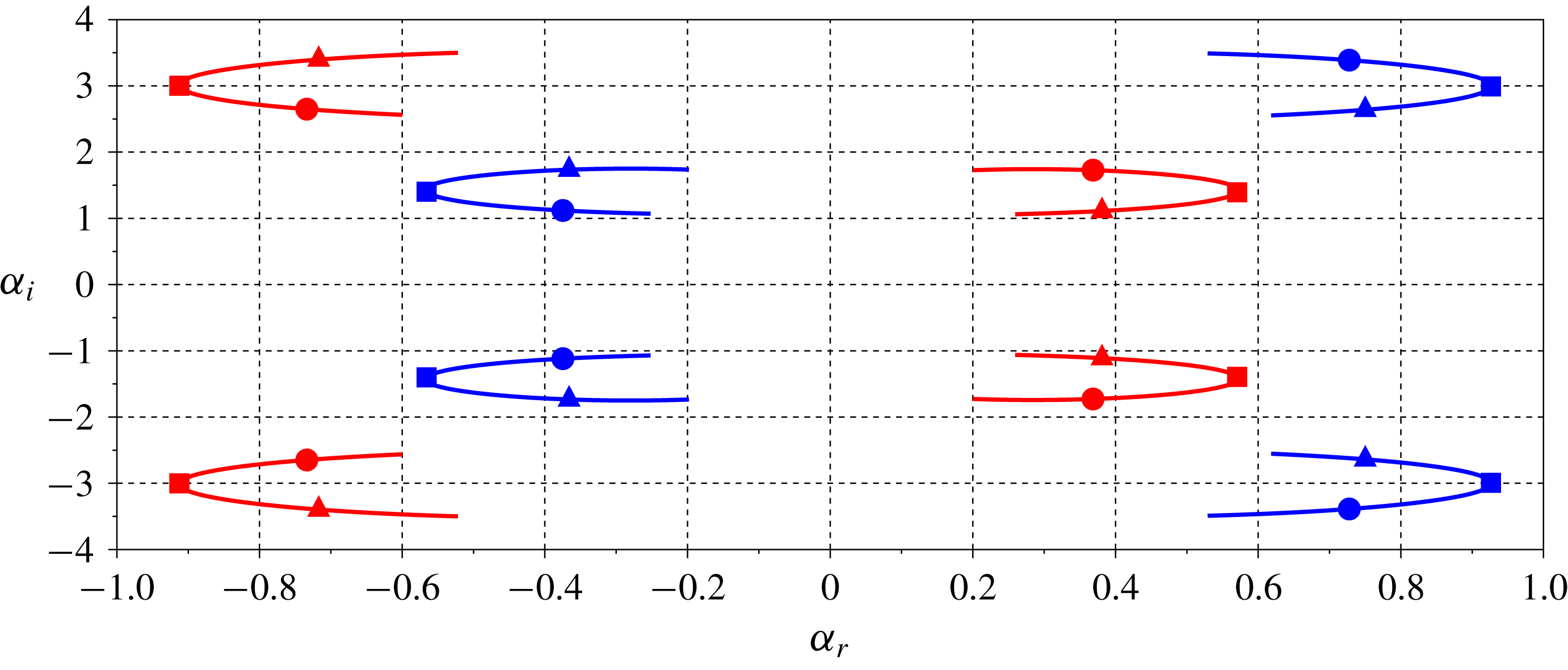
were obtained by making small increments on it and using previous results as initial guesses. As in Jendoubi & Strykowski (Reference Jendoubi and Strykowski1994), many of saddle points were found, each comprising the KH branch and an acoustic-mode branch. The locus of eight of these saddles with
 $V_{ref}$
, defined in (2.2), are shown in figure 23. For all parameters studied the dominant saddle was formed by the first harmonic acoustic mode.
Saddles in the first and third quadrant were found to be formed by a pair of upstream- or a pair of downstream-travelling modes, and thus are not relevant in the impulse response calculation (Huerre & Monkewitz Reference Huerre and Monkewitz1990; Huerre et al. Reference Huerre, Batchelor, Moffatt and Worster2000). Saddles of the second and fourth quadrants are the relevant ones, showing a more complex behaviour.
For
 $V_{ref}<0.5$
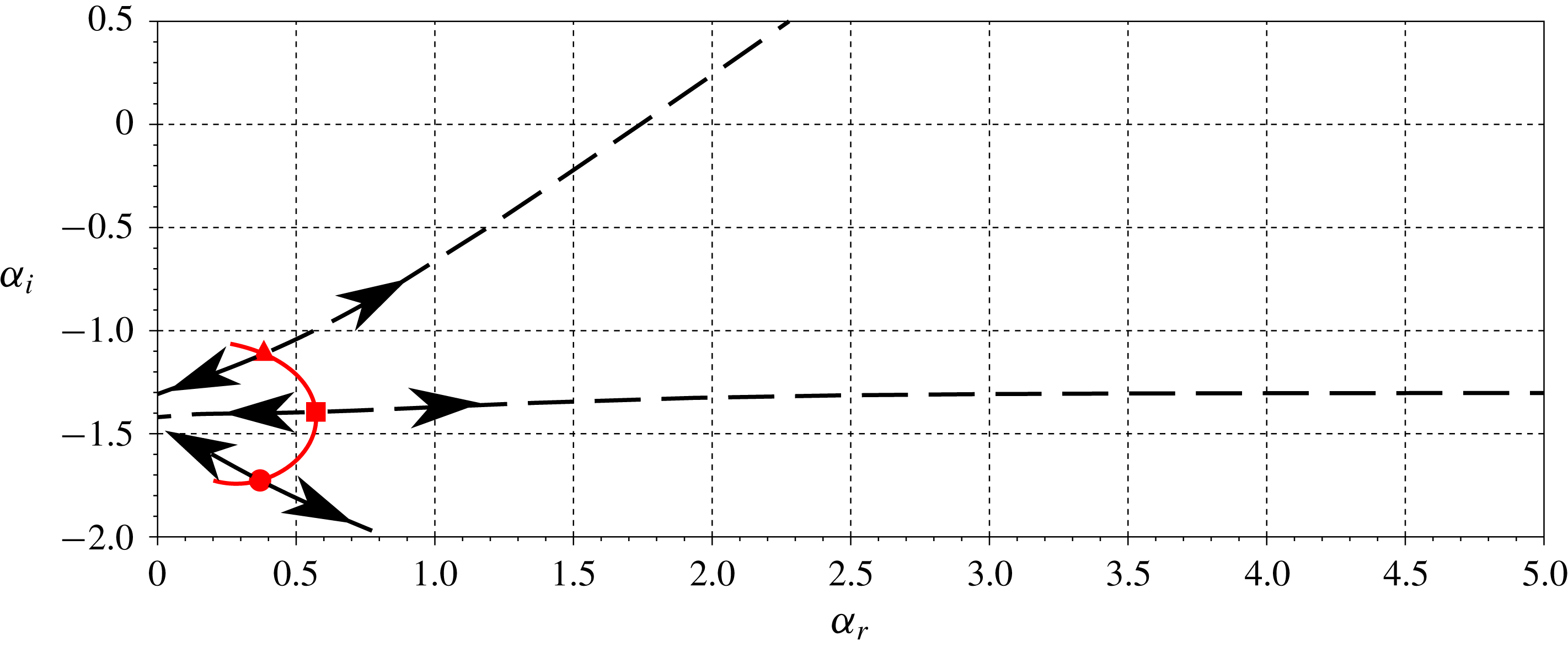
fourth quadrant saddles are formed by an upstream and a downstream mode. However when
 $V_{ref}=0.5$
the downstream mode becomes an upstream mode, thus the saddle is suddenly not ‘valid’ anymore. This process is illustrated in figure 24. A similar but opposite behaviour is found in the second quadrant, for
 $V_{ref}<0.5$
the saddles are all formed by two upstream modes, with one upstream mode becoming a downstream mode at
 $V_{ref}=0.5$
.
This phenomenon is connected to KHs mode group velocity, which can be related to the mean of inner and outer flow speeds. Clearly, for
 $V_{ref}=0$
, the KH mode travels towards positive
 $x$
for the ideal wake, but for
 $V_{ref}=1$
the same mode travels towards negative
 $x$
for the left-pointing jet. At
 $V_{ref}=0.5$
the KH transitions from a upstream- to an downstream-travelling mode, invalidating one saddle and validating the other. This leads to a discontinuities in growth rates of both symmetric and antisymmetric pseudo-wavepacket, as seen in figure 19. This discontinuities are a consequence of the zero-thickness shear layers, disappearing when finite shear layers are considered, as explored in § 5.2.
Loci of eight DVS saddles point with increasing
 $V_{ref}$
. Symmetric and antisymmetric mode saddles in blue and red. The triangle, square and circle markers correspond to
 $V_{ref}=0$
, 0.5 and 1.0.

Briggs criteria for fourth quadrant saddle points for different
 $V_{ref}$
. Red line represents the saddle-point locus, black dashed lines show the path for both of the saddle roots with increasing
 $\unicode[STIX]{x1D714}_{i}$
, with arrows indicating direction of increasing
 $\unicode[STIX]{x1D714}_{i}$
.

B.2 Finite shear-layer thickness wavepacket
Finite shear-layer effects are studied with profiles given by
 $$\begin{eqnarray}U(y)=(U_{in}-U_{out})\left(\frac{\tanh \left({\displaystyle \frac{y+1}{\unicode[STIX]{x1D6FF}}}\right)+\tanh \left(-{\displaystyle \frac{y-1}{\unicode[STIX]{x1D6FF}}}\right)}{2\tanh \left({\displaystyle \frac{1}{\unicode[STIX]{x1D6FF}}}\right)}\right)+U_{out},\end{eqnarray}$$
where
 $\unicode[STIX]{x1D6FF}$
controls the thickness of the mixing layer. The DVS model is recovered by when
 $\unicode[STIX]{x1D6FF}\rightarrow 0$
. Pseudo-spectral methods using Chebyshev polynomials and Gauss–Lobatto points in order to obtain the derivatives at a point and standard generalised eigenvalue routines were used, as in Ormonde et al. (Reference Ormonde, Cavalieri, da Silva and Avelar2018). Two consecutive mappings were used in order to improve vortex-sheet resolution,
 $$\begin{eqnarray}\displaystyle & \displaystyle f_{1}(y)=L\frac{y}{\sqrt{1-y^{2}}}, & \displaystyle\end{eqnarray}$$
 $$\begin{eqnarray}\displaystyle & \displaystyle f_{2}^{-1}(y)=y+a_{2}\left(\tanh \left({\displaystyle \frac{y-1}{a_{1}}}\right)+\tanh \left({\displaystyle \frac{y+1}{a_{1}}}\right)\right), & \displaystyle\end{eqnarray}$$
with
 $L=2$
,
 $a_{1}=1.2\unicode[STIX]{x1D6FF}$
,
 $a_{2}=2$
. The mapping given by
 $f_{1}$
corresponds to the transformation from Chebyshev to rational Chebyshev polynomials, and by
 $f_{2}$
concentrates collocation points around the vortex sheets. The impulse response was obtained by looking for saddle points in the complex
 $\unicode[STIX]{x1D6FC}$
plane. Different runs were made varying
 $\unicode[STIX]{x1D714}_{(r,i)}$
between
 $\unicode[STIX]{x1D714}_{g,(r,i)}\pm 0.05$
, where
 $\unicode[STIX]{x1D714}_{g}$
is the approximate saddle location. Saddle wavenumber (
 $\unicode[STIX]{x1D6FC}_{0}$
) and frequency (
 $\unicode[STIX]{x1D714}_{0}$
) were estimated by a second-order fit of
 $\unicode[STIX]{x1D714}$
and
 $\unicode[STIX]{x1D6FC}$
values of the roots closer to the estimated saddle position.
The locus of saddle points as a function of
 $V_{ref}$
for two shear-layer thicknesses,
 $\unicode[STIX]{x1D6FF}=0.05$
and 0.1, is shown in figure 25. Two types of saddle can be observed. Column saddles occurs for low
 $|\unicode[STIX]{x1D6FC}|$
on both thicknesses and scale with the distance between shear layers. Shear-layer saddles scales with shear-layer thickness, occurring for larger values of
 $|\unicode[STIX]{x1D6FC}|$
for thin layers.
Saddles loci in the complex
 $\unicode[STIX]{x1D6FC}$
-plane with
 $V_{ref}$
. Blue and red lines indicate ‘valid’ (saddle formed by upstream- and downstream-travelling modes) symmetric and antisymmetric modes. Black lines indicate invalid saddles. For small values of
 $\unicode[STIX]{x1D6FF}$
there is a clear distinction between columns and shear-layer saddles.

The shear-layer saddles corresponds to finite-thickness single vortex-sheet saddles, first studied by Huerre & Monkewitz (Reference Huerre and Monkewitz1985): when
 $\unicode[STIX]{x1D6FF}\ll 1$
, they occur for
 $|\text{Re}(\unicode[STIX]{x1D6FC})|\gg 1$
, and thus the wavelength is much smaller than the distance between shear layers, effectively decoupling their behaviour and recovering single vortex-sheet results, which is reflected by similar growth rates of symmetric and antisymmetric absolute instabilities. The range of
 $V_{ref}$
where the shear-layer saddle dominates has counterflow in the shear layer, and thus corresponds to the cases of absolute instability of shear layers due to backflow. Lesshafft & Huerre (Reference Lesshafft and Huerre2007) shear-layer saddles scale with round jet shear-layer thickness, equivalent to results seen in figure 21 for the DVS model.
Appendix C. Free vibration of a string with discontinuous density
A vibrating string obeys the following equation
 $$\begin{eqnarray}\frac{\unicode[STIX]{x2202}^{2}f}{\unicode[STIX]{x2202}t^{2}}(y,t)+\frac{T}{\unicode[STIX]{x1D70C}(y)}\frac{\unicode[STIX]{x2202}^{2}f}{\unicode[STIX]{x2202}y^{2}}(y,t)=0,\end{eqnarray}$$
where
 $f$
is the string displacement and
 $T$
is the string tension, which is constant in the absence of external forcing. We consider here a model where
 $$\begin{eqnarray}\unicode[STIX]{x1D70C}(x)=\left\{\begin{array}{@{}ll@{}}\unicode[STIX]{x1D70C}_{out},\quad & |y|>1\\ \unicode[STIX]{x1D70C}_{int},\quad & |y|<1.\end{array}\right.\end{eqnarray}$$
We can solve the equation on each of the three domains (
 $y<1,|y|<1$
and
 $y>1$
) and then patch the solutions using as interface conditions the continuity of string displacement and force balance,
 $$\begin{eqnarray}f(+1^{+},t)=f(+1^{-},t),\quad T\frac{\unicode[STIX]{x2202}f}{\unicode[STIX]{x2202}y}(+1^{-},t)=T\frac{\unicode[STIX]{x2202}f}{\unicode[STIX]{x2202}y}(+1^{+},t),\end{eqnarray}$$
 $$\begin{eqnarray}f(-1^{+},t)=f(-1^{-},t),\quad T\frac{\unicode[STIX]{x2202}f}{\unicode[STIX]{x2202}y}(-1^{-},t)=T\frac{\unicode[STIX]{x2202}f}{\unicode[STIX]{x2202}y}(-1^{+},t).\end{eqnarray}$$
As boundary conditions we use that for
 $|y|\rightarrow \infty$
we retain only waves moving away from the origin. Assuming symmetric disturbances around
 $y=0$
we have as solutions in each domain
 $$\begin{eqnarray}f(x,t)=\left\{\begin{array}{@{}ll@{}}A\text{e}^{-\text{i}\unicode[STIX]{x1D6FC}_{out}y-\text{i}\unicode[STIX]{x1D714}t},\quad & y>1\\ \cos (\unicode[STIX]{x1D6FC}_{in}y)\text{e}^{-\text{i}\unicode[STIX]{x1D714}t},\quad & 0<y<1,\end{array}\right.\end{eqnarray}$$
where
 $\unicode[STIX]{x1D6FC}_{in}=\unicode[STIX]{x1D714}\sqrt{T/\unicode[STIX]{x1D70C}_{in}}$
and
 $\unicode[STIX]{x1D6FC}_{out}=\unicode[STIX]{x1D714}\sqrt{T/\unicode[STIX]{x1D70C}_{out}}$
. Using the interface conditions we arrive at the dispersion relation
 $$\begin{eqnarray}\displaystyle & \displaystyle \tan (\unicode[STIX]{x1D6FC}_{in})=\text{i}\left(\frac{\unicode[STIX]{x1D70C}_{out}}{\unicode[STIX]{x1D70C}_{in}}\right),\quad \unicode[STIX]{x1D6FC}_{in}=\tan ^{-1}\left(\text{i}\left(\frac{\unicode[STIX]{x1D70C}_{out}}{\unicode[STIX]{x1D70C}_{in}}\right)\right)+n\unicode[STIX]{x03C0}, & \displaystyle\end{eqnarray}$$
 $$\begin{eqnarray}\displaystyle & \displaystyle \unicode[STIX]{x1D6FC}_{out}=\left(\tan ^{-1}\left(\text{i}\left(\frac{\unicode[STIX]{x1D70C}_{out}}{\unicode[STIX]{x1D70C}_{in}}\right)\right)+n\unicode[STIX]{x03C0}\right)\sqrt{{\displaystyle \frac{\unicode[STIX]{x1D70C}_{in}}{\unicode[STIX]{x1D70C}_{out}}}}. & \displaystyle\end{eqnarray}$$
A similar equation is found for the antisymmetric mode, but with a cotangent instead of the tangent function in (C 6) and (C 7).
The amplitude of the outgoing wave is
 $$\begin{eqnarray}A=\frac{\cos (\unicode[STIX]{x1D6FC}_{in})}{\text{e}^{-\text{i}\unicode[STIX]{x1D6FC}_{out}}}.\end{eqnarray}$$
In the limit when
 $\unicode[STIX]{x1D70C}_{in}/\unicode[STIX]{x1D70C}_{out}\rightarrow 0$
,
 $\unicode[STIX]{x1D6FC}_{in}$
tends to
 $(n+1/2)\unicode[STIX]{x03C0}$
, and
 $A\rightarrow 0$
, while when
 $\unicode[STIX]{x1D70C}_{in}/\unicode[STIX]{x1D70C}_{out}\rightarrow \infty$
,
 $|A|\rightarrow 1$
. Interesting aspects of these limits is the emulation of displacement constrains or of force relief constrains at
 $x=\pm 1$
, as seen in figure 11. For finite values of
 $\unicode[STIX]{x1D70C}_{in}/\unicode[STIX]{x1D70C}_{out}$
,
 $\unicode[STIX]{x1D714}$
has a negative imaginary part, indicating a decay of amplitude. When the density ratio is large, the amplitude decay is small because the amplitude of the outgoing waves (A) is small, while on the limit of small density ratio even with unitary amplitude of outgoing waves, the energy of those waves is small when compared with the vibration energy of the inner string.