1 Introduction
The interaction of shock waves and boundary layers is a fundamental problem in high-speed flow physics motivated by practical applications. Dolling (Reference Dolling2001) states ‘(shock-wave boundary-layer interactions) are ubiquitous in high-speed flight, occurring in an almost limitless number of external and internal flow problems relevant to aircraft, missiles, rockets, and projectiles. Maximum mean and fluctuating pressure levels and thermal loads that a structure is exposed to are generally found in regions of shock/boundary-layer and shock/shear-layer interaction and can (affect) vehicle and component geometry, structural integrity, material selection, fatigue life, the design of thermal protection systems, weight, and cost’. Consequently, to better design high-speed vehicles it is necessary to understand the fundamentals of this complex interaction. This ubiquity has led to a plethora of computational (Adams Reference Adams2000; Wu & Martin Reference Wu and Martin2007, Reference Wu and Martin2008; John, Kulkarni & Natarajan Reference John, Kulkarni and Natarajan2014; Wang et al. Reference Wang, Sandham, Hu and Liu2015) and experimental (Settles, Vas & Bogdonoff Reference Settles, Vas and Bogdonoff1976; Settles, Fitzpatrick & Bogdonoff Reference Settles, Fitzpatrick and Bogdonoff1979; Smits & Muck Reference Smits and Muck1987; Humble, Scarano & van Oudheusden Reference Humble, Scarano and van Oudheusden2007; Humble et al. Reference Humble, Elsinga, Scarano and van Oudheusden2009; Giepman, Schrijer & van Oudheusden Reference Giepman, Schrijer and van Oudheusden2015) investigations into this interaction. Reviews (Settles Reference Settles and Dodson1994; Knight et al. Reference Knight, Yan, Panaras and Zheltovodov2003; Gaitonde Reference Gaitonde2015) highlight the current state of the research.
The breadth of interactions is vast, as discussed in the introductory chapters of Babinsky & Harvey (Reference Babinsky and Harvey2011). In this work, we focus our study on the effect of the compression-corner angle on the streamwise turbulent kinetic energy (sTKE) and structure in Mach 2.8 flow. For example, this canonical flow may be observed in practice as the deflection of a control surface on a vehicle in high-speed flight or in the flow path of a high-speed, air-breathing engine. Trends of velocity-fluctuation amplitude and turbulence structure with compression-corner angle imply a change in the shear stress, heat-transfer rate and mixing properties of the flow, all of which have simulation and design implications.
An important feature of shock-wave/boundary-layer interaction (SWBLI) is the modification of turbulence stresses across the flow field. Experimental investigations have determined that there is significant amplification of turbulence across shocks. Smits & Muck (Reference Smits and Muck1987) studied the shock-wave/turbulent boundary-layer interaction over three compression corners and reported amplification factors of 4–15 for the mass-flux fluctuation intensity, and even larger factors for the shear stresses. Humble et al. (Reference Humble, Scarano and van Oudheusden2007) used particle image velocimetry (PIV) to study the flow over a flat plate with an impinging shock and found amplification factors of the same order of magnitude as Smits & Muck (Reference Smits and Muck1987). Computational efforts have also provided similar insight. In the direct numerical simulation (DNS) of Wu & Martin (Reference Wu and Martin2007), amplification factors of 6–24 for the Reynolds stresses were calculated for a Mach 2.9 flow over a
 $24^{\circ }$
compression ramp. Using large eddy simulation (LES), Porter & Poggie (Reference Porter and Poggie2017) reported amplification factors of 2.3–7.6 for the Reynolds stresses for a Mach 2.25 flow over a
 $24^{\circ }$
compression ramp.
Another important feature of turbulent flow is the existence of structures of various time and length scales (Tennekes & Lumley Reference Tennekes and Lumley1972). The interaction of this wide range of turbulent scales with a shock wave yields a rich, fundamental fluid-mechanics problem. Being able to quantify these scales and deepening our understanding of the physical properties and relative importance of these structures will further improve our ability to model turbulent flows. One analytical tool that accomplishes this is proper orthogonal decomposition (POD). It was first introduced to the fluid dynamics community by Lumley (Lumley Reference Lumley, Yaglom and Tatarsky1967; Berkooz, Holmes & Lumley Reference Berkooz, Holmes and Lumley1993) as a means to extract coherent structures from flow fields. A review of POD analysis in the broader context of modal analysis can be found in Taira et al. (Reference Taira, Brunton, Dawson, Rowley, Colonius, McKeon, Schmidt, Gordeyev, Theofilis and Ukeiley2017). The fundamental idea of POD is to decompose the velocity field into a series of modes weighted based on the amount of kinetic energy they contain, each of which can be interpreted as a coherent structure. This technique has been used to study combustion engines (Druault, Guibert & Alizon Reference Druault, Guibert and Alizon2005; Chen, Reuss & Sick Reference Chen, Reuss and Sick2012; Chen et al. Reference Chen, Reuss, Hung and Sick2013), turbulent flow over a fence (Orellano & Wengle Reference Orellano and Wengle2001), open cavity flow (Murray, Sällström & Ukeiley Reference Murray, Sällström and Ukeiley2009), axisymmetric jet flow and mixing layers (Bonnet et al. Reference Bonnet, Cole, Delville, Glauser and Ukeiley1994) and the turbulent flow over a cylinder (Tu et al. Reference Tu, Rowley, Kutz and Shang2014), to name a few. There are not many applications of POD to SWBLIs in the literature. One example is that of Piponniau et al. (Reference Piponniau, Collin, Dupont and Debiève2012) where a POD analysis was performed on PIV results from an induced-shock-wave/turbulent boundary-layer interaction. The authors aimed to investigate ‘the unsteady breathing of the recirculating bubble at low frequency and the Kelvin-Helmholtz instabilities developing at moderate frequency’.
We begin this paper by describing the experimental facility, the Mach 3 Calibration Tunnel (the M3CT) and the measurement technique, krypton tagging velocimetry (KTV). Then, we establish that the incoming flow is nominally a canonical supersonic, turbulent boundary layer over a flat plate by reporting KTV measurements of mean- and fluctuating-velocity profiles and comparing them to those found in the literature. We then report results of mean- and fluctuating-velocity profiles of flows over
 $8^{\circ }$
,
 $16^{\circ }$
,
 $24^{\circ }$
and
 $32^{\circ }$
compression corners which yields a case-wise comparison of streamwise turbulent kinetic energy (sTKE). Finally, we apply POD to the KTV results and discuss the eigenspectra and make case-wise comparisons of the most energetic POD modes.
2 Facility and experimental set-up
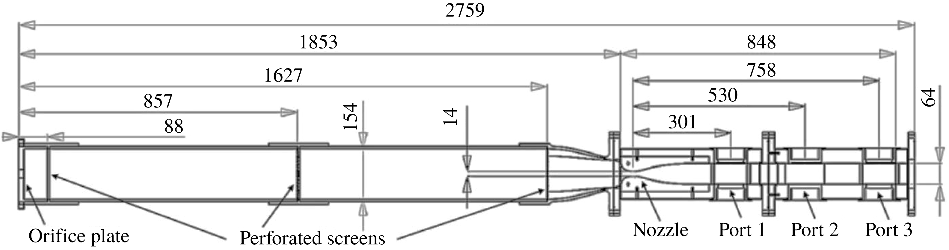
The experiments were performed in the Arnold Engineering Development Complex (AEDC) Mach 3 Calibration Tunnel (M3CT) in Silver Spring, MD (figure 1). The tunnel is comprised of a large vacuum tank attached to a converging diverging nozzle. An orifice plate was added upstream of the nozzle as in Zahradka et al. (Reference Zahradka, Parziale, Smith and Marineau2016a
) and Mustafa et al. (Reference Mustafa, Hunt, Parziale, Smith and Marineau2017a
) to control the free-stream pressure. A flexible isolation bag was added upstream of the orifice to contain the 99 %
 $\text{N}_{2}/1\,\%~\text{Kr}$
gas mixture. The flexibility ensured that the bag stayed at the constant ambient pressure of the laboratory. A valve is cycled downstream of the nozzle to run the tunnel. The run condition calculations can be found in Zahradka et al. (Reference Zahradka, Parziale, Smith and Marineau2016a
) and Mustafa et al. (Reference Mustafa, Hunt, Parziale, Smith and Marineau2017a
) (table 1).
Sketch of AEDC Mach 3 Calibration Tunnel (M3CT). Dimensions in millimetres. The measurements are made at ‘Port 2’.

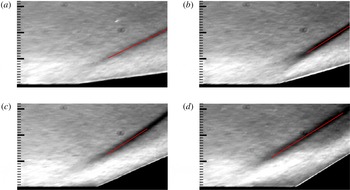
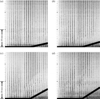
Mean schlieren images for the (a)
 $8^{\circ }$
, (b)
 $16^{\circ }$
, (c)
 $24^{\circ }$
and (d)
 $32^{\circ }$
corners, respectively. Flow is left to right. Major tick marks are at 10 mm. Incoming boundary-layer thickness is
 $\unicode[STIX]{x1D6FF}=10.25~\text{mm}$
. Mean shock position shown in red.

Values of
 $M_{\infty }$
,
 $P_{\infty }$
,
 $T_{\infty }$
,
 $\unicode[STIX]{x1D70C}_{\infty }$
,
 $Re_{\infty }^{unit}$
,
 $Re_{\unicode[STIX]{x1D6E9}}$
,
 $U_{\infty }$
and
 $\unicode[STIX]{x1D6FF}$
are the Mach number, pressure, temperature, density, unit Reynolds number, momentum-thickness Reynolds number, velocity and boundary-layer thickness for the AEDC M3CT tunnel with the 19.1 mm orifice plate. Additionally,
 $u_{\unicode[STIX]{x1D70F}}$
,
 $\unicode[STIX]{x1D708}_{w}$
and
 $\unicode[STIX]{x1D702}$
are the friction velocity, kinematic viscosity at the wall and the viscous length, respectively. Values reported here are for ‘Port 2’ in figure 1.

To ensure that the M3CT started properly and to visualize the shock-wave/turbulent boundary-layer interaction structures, a Z-type schlieren set-up (Settles Reference Settles2001) was used to visualize the flow field over the compression corners. The schlieren set-up consisted of a sparklamp light source and an Integrated Design Tools N3 camera recording at 100 frames-per-second with a 50 ns exposure time. The knife edge was set as a horizontal cutoff. Figure 2 shows the mean of 100 exposures of the schlieren visualization for each wedge with the mean shock position marked, as determined by local curve fitting to the image intensity. Approximately 900 snapshots of data were collected for each geometry, which corresponds to a physical time of 90 s.
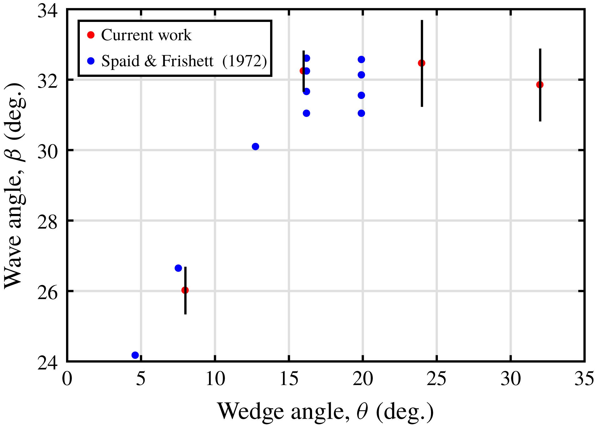
To compare the flow field investigated in the present work with that in the literature, the mean initial shock angles (
 $\unicode[STIX]{x1D6FD}$
) are plotted in figure 3 against the wedge angle
 $\unicode[STIX]{x1D703}$
. The graph shows that for the
 $8^{\circ }$
wedge,
 $\unicode[STIX]{x1D6FD}$
is equal to the calculated value from inviscid theory. Beginning with the
 $16^{\circ }$
wedge,
 $\unicode[STIX]{x1D6FD}$
approaches a constant value of
 ${\approx}32^{\circ }$
. This trend of
 $\unicode[STIX]{x1D6FD}$
approaching a constant value is in agreement with the work by Spaid & Frishett (Reference Spaid and Frishett1972), which was experimental work performed at Mach 2.9. The value of
 $\unicode[STIX]{x1D6FD}$
for the
 $8^{\circ }$
and
 $16^{\circ }$
wedge is in agreement with previous work by Smits & Muck (Reference Smits and Muck1987). The initial shock angle for the
 $24^{\circ }$
wedge is in agreement with DNS work by Wu & Martin (Reference Wu and Martin2007) and experimental work by Settles et al. (Reference Settles, Vas and Bogdonoff1976) and Mustafa et al. (Reference Mustafa, Hunt, Parziale, Smith and Marineau2017a
). From the comparison of the initial shock angle with those in the literature, we conclude that the flow has started and these geometries can be studied in the M3CT. In addition to shock angle, we show the extent of flow separation for each corner angle as a distribution of the instantaneous normalized velocity at the root (figure 11).
Initial (
 $\unicode[STIX]{x1D6FD}$
) shock angles from schlieren images shown in red. Results from Spaid & Frishett (Reference Spaid and Frishett1972) shown in blue. Vertical black bars denote uncertainty.

3 Diagnostic approach: tagging velocimetry
Tagging velocimetry is a laser velocimetry technique which is typically performed in gases by tracking the fluorescence of a native, seeded or synthesized gas. Its advantage over particle-based techniques in high-speed facilities is that it is not limited by timing issues associated with tracer injection (Haertig et al. Reference Haertig, Havermann, Rey and George2002) or reduced particle response at Knudsen and Reynolds numbers (Loth Reference Loth2008) characteristic of high-speed wind tunnels. Methods of tagging velocimetry include the VENOM (Hsu et al. Reference Hsu, Srinivasan, Bowersox and North2009a ,Reference Hsu, Srinivasan, Bowersox and North b ; Sánchez-González et al. Reference Sánchez-González, Srinivasan, Bowersox and North2011; Sánchez-González, Bowersox & North Reference Sánchez-González, Bowersox and North2012, Reference Sánchez-González, Bowersox and North2014), APART (Dam et al. Reference Dam, Klein-Douwel, Sijtsema and ter Meulen2001; Sijtsema et al. Reference Sijtsema, Dam, Klein-Douwel and ter Meulen2002; Van der Laan et al. Reference Van der Laan, Tolboom, Dam and ter Meulen2003), RELIEF (Miles et al. Reference Miles, Cohen, Connors, Howard, Huang, Markovitz and Russell1987, Reference Miles, Connors, Markovitz, Howard and Roth1989, Reference Miles, Zhou, Zhang and Lempert1993; Miles & Lempert Reference Miles and Lempert1997; Miles et al. Reference Miles, Grinstead, Kohl and Diskin2000), FLEET (Michael et al. Reference Michael, Edwards, Dogariu and Miles2011; Edwards, Dogariu & Miles Reference Edwards, Dogariu and Miles2015), STARFLEET (Jiang et al. Reference Jiang, Halls, Stauffer, Danehy, Gord and Roy2016), PLEET (Jiang et al. Reference Jiang, Mance, Slipchenko, Felver, Stauffer, Yi, Danehy and Roy2017), argon (Mills Reference Mills2016), iodine (McDaniel, Hiller & Hanson Reference McDaniel, Hiller and Hanson1983; Balla Reference Balla2013), sodium (Barker, Bishop & Rubinsztein-Dunlop Reference Barker, Bishop and Rubinsztein-Dunlop1997), acetone (Lempert et al. Reference Lempert, Jiang, Sethuram and Samimy2002, Reference Lempert, Boehm, Jiang, Gimelshein and Levin2003; Handa et al. Reference Handa, Mii, Sakurai, Imamura, Mizuta and Ando2014), NH (Zhang et al. Reference Zhang, Yu, Yan, Huang and Liu2017) and the hydroxyl group techniques, (Boedeker Reference Boedeker1989; Wehrmeyer et al. Reference Wehrmeyer, Ribarov, Oguss and Pitz1999; Pitz et al. Reference Pitz, Lahr, Douglas, Wehrmeyer, Hu, Carter, Hsu, Lum and Koochesfahani2005; André et al. Reference André, Bardet, Burns and Danehy2017) among others (Hiller et al. Reference Hiller, Booman, Hassa and Hanson1984; Gendrich & Koochesfahani Reference Gendrich and Koochesfahani1996; Gendrich, Koochesfahani & Nocera Reference Gendrich, Koochesfahani and Nocera1997; Ribarov et al. Reference Ribarov, Wehrmeyer, Batliwala, Pitz and DeBarber1999; Stier & Koochesfahani Reference Stier and Koochesfahani1999; André et al. Reference André, Burns, Danehy, Cadell, Woods and Bardet2018).
For this work, krypton tagging velocimetry (KTV) was used as the velocimetry technique. The use of a metastable noble gas as a tagging velocimetry tracer was first suggested by Mills, Sukenik & Balla (Reference Mills, Sukenik and Balla2011) and Balla & Everhart (Reference Balla and Everhart2012). KTV was first demonstrated by Parziale, Smith & Marineau (Reference Parziale, Smith and Marineau2015a
,Reference Parziale, Smith and Marineau
b
) to measure the velocity along the centreline of an underexpanded jet of an
 $\text{N}_{2}/\text{Kr}$
mixture. Following that work, Zahradka et al. (Reference Zahradka, Parziale, Smith and Marineau2016a
,Reference Zahradka, Parziale, Smith and Marineau
b
) used KTV to make measurements of the mean and fluctuating turbulent boundary-layer profiles in a Mach 2.8 flow. Mustafa et al. (Reference Mustafa, Hunt, Parziale, Smith and Marineau2017a
) used KTV to measure seven simultaneous profiles of streamwise velocity and fluctuations in the incoming boundary layer and immediately upstream of a
 $24^{\circ }$
compression corner in a
 $M_{\infty }=2.8$
,
 $Re_{\unicode[STIX]{x1D6E9}}=1750$
, 99 %
 $\text{N}_{2}/1\,\%~\text{Kr}$
shock-wave/turbulent boundary-layer interaction. Recently, KTV was implemented in the Stevens Institute of Technology Shock Tube by Mustafa & Parziale (Reference Mustafa and Parziale2017) to measure the free-stream velocity behind a Mach 3 shock. In addition, KTV has been demonstrated to work in the free stream of the large-scale AEDC Hypervelocity Tunnel 9 at Mach 10 and Mach 14 (Mustafa et al.
Reference Mustafa, Parziale, Smith and Marineau2017b
). Finally, preliminary two-dimensional KTV measurements in a Mach 2.8 flow over a
 $24^{\circ }$
compression corner were reported in Mustafa et al. (Reference Mustafa, Parziale, Smith and Marineau2018) and simplifications to the technique are reported in Mustafa & Parziale (Reference Mustafa and Parziale2018).
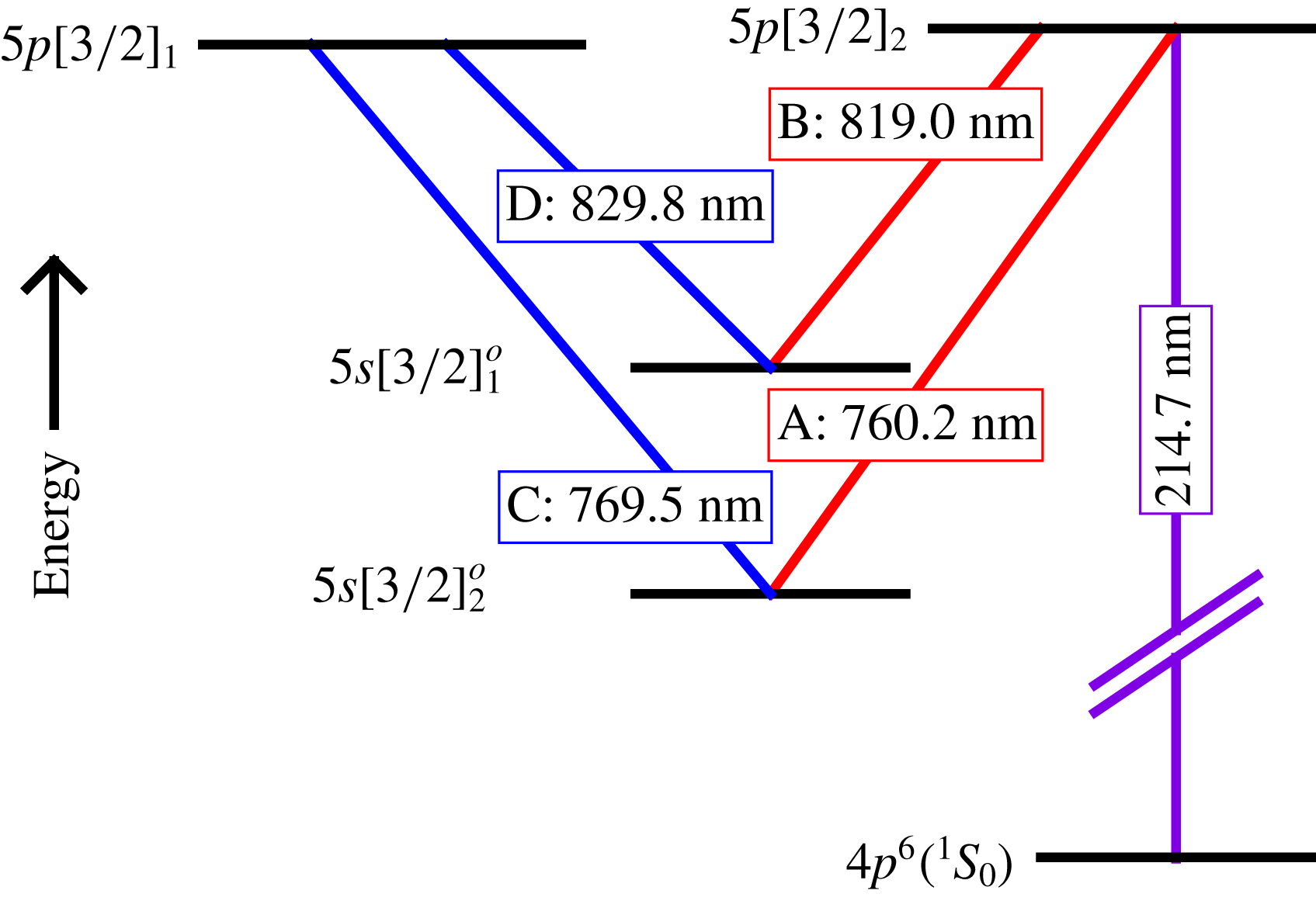
Energy diagram for excitation scheme. Racah
 $\text{nl}[\text{K}]_{J}$
notation, A, B, C and D represent the transitions between the states.

Following the excitation scheme used by Mustafa et al. (Reference Mustafa, Hunt, Parziale, Smith and Marineau2017a ), KTV is performed in the following steps according to the energy level diagram shown in figure 4.
(i) Seed a base flow with krypton globally, in this case 1 % Kr in 99 %
 $\text{N}_{2}$
.
(ii) Photosynthesize metastable krypton atoms with a pulsed tuneable laser to form the tagged tracer: two-photon excitation of
$4p^{6}(\text{}^{1}\text{S}_{0})\rightarrow 5p[3/2]_{2}$
(214.7 nm) and rapid decay to resonance state
$5p[3/2]_{2}\rightarrow 5s[3/2]_{1}^{o}$
(819.0 nm, transition B) and metastable state
$5p[3/2]_{2}\rightarrow 5s[3/2]_{2}^{o}$
(760.2 nm, transition A). We estimate that the creation of the metastable atoms which comprise the ‘write line’ takes approximately 50 ns Chang, Horiguchi & Setser (Reference Chang, Horiguchi and Setser1980). The position of the write line is marked by the fluorescence from the
$5p[3/2]_{2}\rightarrow 5s[3/2]_{1}^{o}$
transitions (819.0 nm, transition B), and is recorded with a camera positioned normal to the flow.(iii) Record the displacement of the tagged metastable krypton by imaging the laser induced fluorescence (LIF) that is produced with an additional pulsed tuneable laser: excite
$5p[3/2]_{1}$
level by
$5s[3/2]_{2}^{o}\rightarrow 5p[3/2]_{1}$
transition with laser sheet (769.5 nm, transition C) and read spontaneous emission of
$5p[3/2]_{1}\rightarrow 5s[3/2]_{1}^{o}$
(829.8 nm, transition D) transitions with a camera positioned normal to the flow.








The experiments were run using two tuneable lasers to provide the 214.7 nm (write) and 769.5 nm (read) laser beams required for KTV. The write laser consisted of a frequency doubled Quanta Ray Pro-350 Nd:YAG laser and a frequency tripled Sirah PrecisionScan Dye Laser. The Nd:YAG laser pumped the dye laser with
 $1000~\text{mJ}~\text{pulse}^{-1}$
at a wavelength of 532 nm. The dye in the laser was DCM with a dimethyl sulfoxide (DMSO) solvent, and the laser was tuned to output a 644.1 nm beam. Frequency tripling of the dye-laser output was performed using Sirah tripling optics (THU 205).
The write-laser beam set-up can result in approximately
 $10{-}13~\text{mJ}~\text{pulse}^{-1}$
; however, approximately 7 mJ was used for this experiment by reducing the Nd:YAG pump-laser power. The wavelength was 214.7 nm, with a linewidth of approximately
 $0.045~\text{cm}^{-1}$
, a pulse width of approximately 7 ns and a repetition rate of 10 Hz. The write beam was focused into several narrow waists in the test section with a
 $f=100~\text{mm}$
fused-silica microlens array (SUSS MicroOptics Nr. 18-00127) to form the lines in the streamwise direction and a
 $f=100~\text{mm}$
fused-silica cylindrical lens to focus the lines in the spanwise direction. We estimate that the energy per write line was approximately
 $350~\unicode[STIX]{x03BC}\text{J}~\text{pulse}^{-1}$
.
The read laser consisted of a frequency doubled Quanta Ray Pro-350 Nd:YAG laser and a Sirah PrecisionScan Dye Laser. The Nd:YAG laser pumped the dye laser with
 $200~\text{mJ}~\text{pulse}^{-1}$
at a wavelength of 532 nm. The dye in the laser was Styryl 8 with a DMSO solvent, and the laser was tuned to output a 769.5 nm beam.
The read-laser beam set-up resulted in approximately
 $5~\text{mJ}~\text{pulse}^{-1}$
, with a wavelength of 769.5 nm, a linewidth of approximately
 $0.025~\text{cm}^{-1}$
, a pulse width of approximately 7 ns and a repetition rate of 10 Hz. The read-laser beam was directed into the test section using 2 inch broadband dielectric mirrors (Thorlabs BB2-E02), and expanded to a beam of
 ${\approx}40~\text{mm}$
diameter with a
 $f=-400~\text{mm}$
BK7 lens. This ‘read beam’ re-excited the metastable Kr tracer atoms so that their displacement could be measured.
The laser and camera timing were controlled by a pulse-delay generator (SRS DG645). The intensified camera used for all experiments was a 16-bit Princeton Instruments PIMAX-4
 $1024\times 1024$
with an 18 mm grade 1, Gen III extended red filmless intensifier w/P46 phosphor (PM4-1024i-HR-FG-18-P46-CM). The lens used is a Nikon NIKKOR 24–85 mm f/2.8-4D in ‘macro’ mode and positioned approximately 200 mm from the write/read location which was at the centre of the test section at Port 2 in figure 1. Two high-precision 800 nm longpass filters (Thorlabs FELH0800, transmission of 3.5e-4 % at the read-laser wavelength of 769.5 nm) were placed in series between the lens and the intensifier to minimize the noise resulting from the read-laser pulse reflection and scatter from solid surfaces. The gain was set to 100 % with
 $1\times 6$
(streamwise
 $\times$
wall-normal) pixel binning and only recording the read images to ensure a 10 Hz frame rate. A set of write images were recorded with the tunnel on prior to each set of experiments. The camera gate was opened for 20 ns immediately following the read-laser pulse to capture the spontaneous emission of
 $5p[3/2]_{1}\rightarrow 5s[3/2]_{1}^{o}$
(829.8 nm) transitions.
4 Boundary-layer results
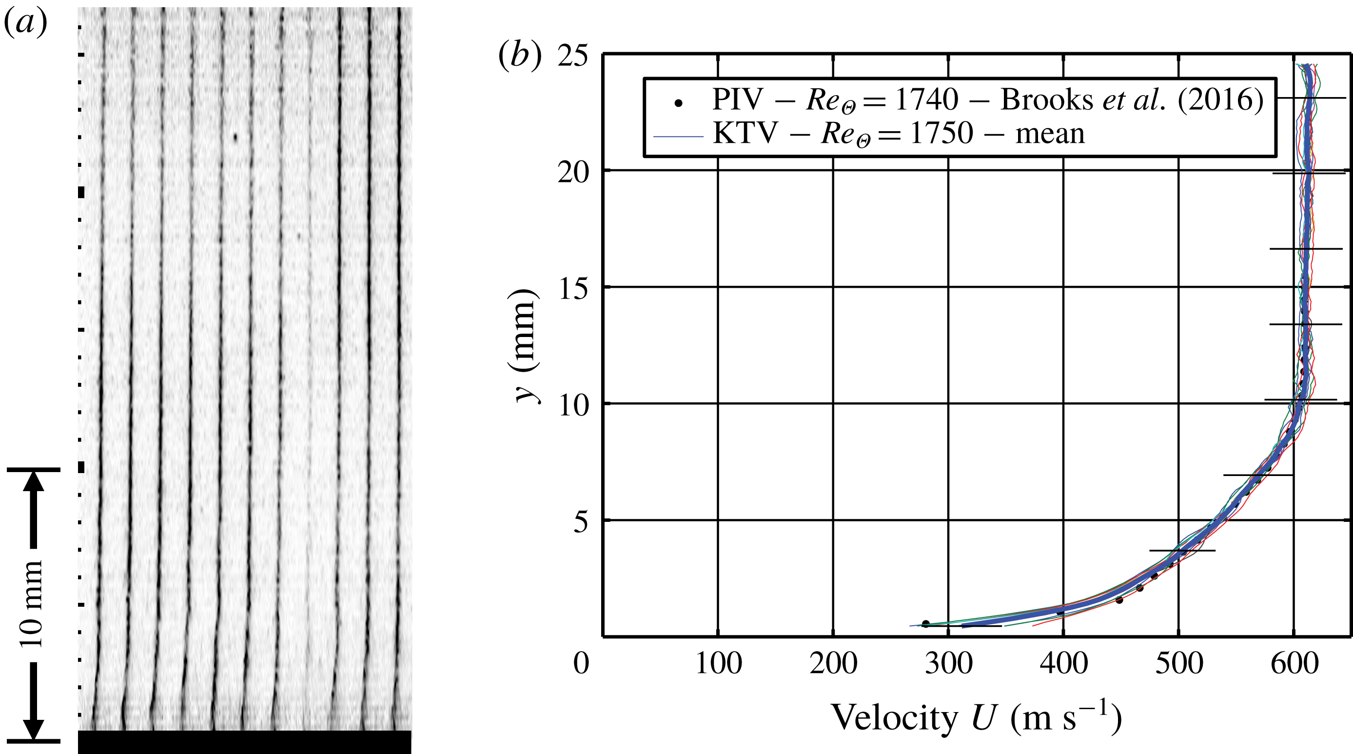
In this section, we present a baseline boundary-layer profile of streamwise velocity and fluctuations. For the boundary-layer results, the write/read delay was set to 500 ns. The KTV set-up formed ten lines with appropriate signal to noise ratio (SNR). A sample read exposure is presented in figure 5(a). To process the KTV exposures, the line centres were found in the following way:
(i) Crop the image to an appropriate field of view.
(ii) Apply a two-dimensional Wiener adaptive-noise removal filter.
(iii) Convert the images to double precision numbers and normalize the intensity to fall in the range of 0–1.
(iv) Apply the Gaussian peak finding algorithm from O’Haver (Reference O’Haver1997) to find the line centres for the top row using the read lines in the top row of each image as a first guess.
(v) Proceeding from the top down, apply the Gaussian peak finding algorithm from O’Haver (Reference O’Haver1997) to find the line centres for each row using the line centre location immediately above as the guess.
The dimensional velocity is presented in figure 5(b) as measured by KTV from the present work and PIV from Brooks et al. (Reference Brooks, Gupta, Smith and Marineau2014, Reference Brooks, Gupta, Smith and Marineau2015, Reference Brooks, Gupta, Smith and Marineau2016, Reference Brooks, Gupta, Smith and Marineau2018) in the same facility. Figure 5(b) shows that the boundary-layer thickness in the incoming flow,
 $\unicode[STIX]{x1D6FF}$
, is
 ${\approx}$
10.25 mm. This is the value that is used to normalize the distance coordinates in subsequent figures and analyses. Error bars for the KTV measurements are calculated in the same fashion as Zahradka et al. (Reference Zahradka, Parziale, Smith and Marineau2016a
) as
 $$\begin{eqnarray}\widetilde{U}_{KTV}=\left[\left(\widetilde{\unicode[STIX]{x0394}x}\frac{\unicode[STIX]{x2202}U}{\unicode[STIX]{x2202}\unicode[STIX]{x0394}x}\right)^{2}+\left(\widetilde{\unicode[STIX]{x0394}t}\frac{\unicode[STIX]{x2202}U}{\unicode[STIX]{x2202}\unicode[STIX]{x0394}t}\right)^{2}+\left(v_{rms}^{\prime }\frac{\unicode[STIX]{x2202}U}{\unicode[STIX]{x2202}y}\unicode[STIX]{x0394}t\right)^{2}\right]^{1/2},\end{eqnarray}$$
where uncertainty estimates of a variable are indicated with a tilde.
(a) Example of KTV boundary-layer fluorescence exposure. Major tick marks are 10 mm. Flow is left to right. Inverted intensity scale. Wall marked as black. (b) Dimensional velocity of the Mach 2.8 turbulent boundary layer. Error bars in black.

The uncertainty in the measured displacement distance,
 $\widetilde{\unicode[STIX]{x0394}x}$
, of the metastable tracer is estimated as the 95 % confidence bound on the write and read locations from the Gaussian fits. The uncertainty in time,
 $\widetilde{\unicode[STIX]{x0394}t}$
, is estimated to be the camera gate width, 20 ns, causing fluorescence blurring as considered in Bathel et al. (Reference Bathel, Danehy, Inman, Jones, Ivey and Goyne2011). The third term in (4.1) is the uncertainty in the streamwise velocity due to wall-normal fluctuations in the
 $xy$
-plane. This formulation is taken from Hill & Klewicki (Reference Hill and Klewicki1996) and Bathel et al. (Reference Bathel, Danehy, Inman, Jones, Ivey and Goyne2011). The wall-normal fluctuations used in (4.1) (
 $v_{rms}^{\prime }$
) are conservatively estimated to be 5 % of the edge velocity, which is supported by DNS (Martin Reference Martin2007) and PIV experiments (Brooks et al.
Reference Brooks, Gupta, Smith and Marineau2016).
The error in the KTV measurement is approximately 5 % in the free stream, the boundary-layer wake region and the boundary-layer logarithmic region. The error in KTV measurement increases to approximately 10 % nearest to the wall. The increase nearest to the wall is mostly due to the third term in (4.1). There is an appreciable increase in the wall-normal fluctuations and increase in velocity gradient.
The velocity data for the boundary layer can be compared to the law of the wall in the logarithmic region,
 $U^{+}=(1/\unicode[STIX]{x1D705})\ln (y^{+})+C$
, by using the van Driest I transformation, with
 $y^{+}=\unicode[STIX]{x1D70C}_{w}u_{\unicode[STIX]{x1D70F}}y/\unicode[STIX]{x1D707}_{w}$
and
 $U^{+}=U/u_{\unicode[STIX]{x1D70F}}$
. Following Bradshaw (Reference Bradshaw1977) and Huang & Coleman (Reference Huang and Coleman1994), the van Driest I transformed velocity is written as
 $$\begin{eqnarray}U_{VD}^{+}=\frac{1}{R}\left[\sin ^{-1}\left(\frac{R(U^{+}+H)}{\sqrt{1+R^{2}H^{2}}}\right)-\sin ^{-1}\left(\frac{RH}{\sqrt{1+R^{2}H^{2}}}\right)\right],\end{eqnarray}$$
where
 $R=M_{\unicode[STIX]{x1D70F}}\sqrt{(\unicode[STIX]{x1D6FE}-1)Pr_{t}/2}$
,
 $H=B_{q}/((\unicode[STIX]{x1D6FE}-1)M_{\unicode[STIX]{x1D70F}}^{2})$
,
 $M_{\unicode[STIX]{x1D70F}}=u_{\unicode[STIX]{x1D70F}}/c_{w}$
and
 $B_{q}=q_{w}/(\unicode[STIX]{x1D70C}_{w}c_{p}u_{\unicode[STIX]{x1D70F}}T_{w})$
. We assume the turbulent Prandtl number is
 $Pr_{t}=0.87$
, and, assuming the Reynolds analogy holds, the heat-flux number is
 $B_{q}=c_{f}\unicode[STIX]{x1D70C}_{e}U_{e}(T_{w}-T_{r})/(2Pr_{e}\unicode[STIX]{x1D70C}_{w}u_{\unicode[STIX]{x1D70F}}T_{w})$
(Schlichting Reference Schlichting2000). Here,
 $c_{w}$
is the sound speed at the wall,
 $c_{p}$
is the constant pressure specific heat,
 $T_{w}$
is the wall temperature,
 $T_{e}$
is the edge temperature,
 $T_{r}$
is the recovery temperature,
 $c_{f}$
is the skin friction coefficient,
 $U_{e}$
is the edge velocity,
 $Pr_{e}$
is the edge Prandlt number,
 $\unicode[STIX]{x1D70C}_{w}$
is the density at the wall,
 $\unicode[STIX]{x1D70C}_{e}$
is the edge density,
 $q_{w}$
is the heat transfer rate at the wall and
 $y$
is the ratio of specific heats. The friction velocity,
 $u_{\unicode[STIX]{x1D70F}}$
, is calculated in the same way as Zahradka et al. (Reference Zahradka, Parziale, Smith and Marineau2016a
) using the von Kármán (Reference von Kármán1934)–Schoenherr (Reference Schoenherr1932) equation under the van Driest II transformation (table 1). Based on these values, the viscous length scale is
 $\unicode[STIX]{x1D702}\approx \unicode[STIX]{x1D708}_{w}/u_{\unicode[STIX]{x1D70F}}\approx 40~\unicode[STIX]{x03BC}\text{m}$
. For comparison, the wall-normal spatial resolution of this KTV implementation is
 ${\approx}170~\unicode[STIX]{x03BC}\text{m}$
due to camera resolution. The streamwise spatial resolution for a single KTV line is estimated to be
 ${\approx}10~\unicode[STIX]{x03BC}\text{m}$
, which is the uncertainty in line-centre location. These resolutions approach the viscous length scale in the flow. We should note that the streamwise spatial resolution for tracking turbulent structures as a field (as is the case in the longitudinal correlations and forthcoming POD analysis) is 1.2 mm due to measurement spacing (figure 5).
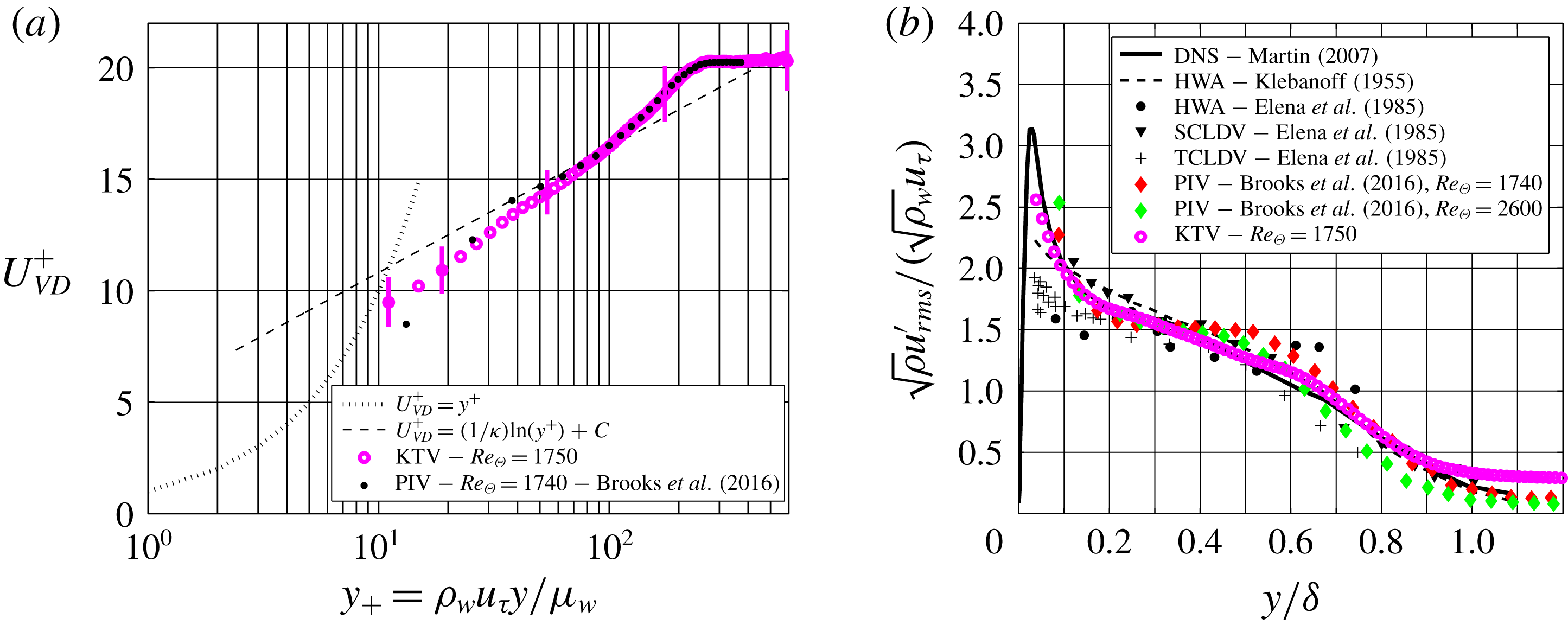
(a) The van Driest scaling of the mean velocity. (b) Morkovin scaling of streamwise fluctuations.

The transformed KTV- and PIV-derived velocity profiles are presented in figure 6(a). Also, in figure 6(a), we plot the viscous sublayer as
 $U_{VD}^{+}=y^{+}$
as well as applying (4.2) to the logarithmic law as
 $$\begin{eqnarray}U_{VD}^{+}=\frac{1}{\unicode[STIX]{x1D705}}\ln (y^{+})+C,\end{eqnarray}$$
with
 $\unicode[STIX]{x1D705}=0.41$
and
 $C=5.2$
. The transformed velocity follows the law of the wall in the logarithmic region with good agreement.
In figure 6(b), we present the streamwise-velocity-fluctuation results that are non-dimensionalized by the Morkovin (Morkovin Reference Morkovin1962) scaling and compare those to the literature (Klebanoff Reference Klebanoff1955; Elena, Lacharme & Gaviglio Reference Elena, Lacharme and Gaviglio1985; Martin Reference Martin2007; Brooks et al.
Reference Brooks, Gupta, Smith and Marineau2016). In this work, we were able to resolve far closer to the wall than in the previous KTV effort by Zahradka et al. (Reference Zahradka, Parziale, Smith and Marineau2016a
). The agreement between the fluctuation data from the literature and KTV is good to down to
 $y/\unicode[STIX]{x1D6FF}\approx 0.05$
.
(a) Longitudinal correlation for
 $y/\unicode[STIX]{x1D6FF}\approx 0.2$
. As a means of first comparison,
 $f_{u^{\prime }u^{\prime }}$
from the present KTV boundary-layer data is compared to
 $f_{(\unicode[STIX]{x1D70C}u)^{\prime }(\unicode[STIX]{x1D70C}u)^{\prime }}$
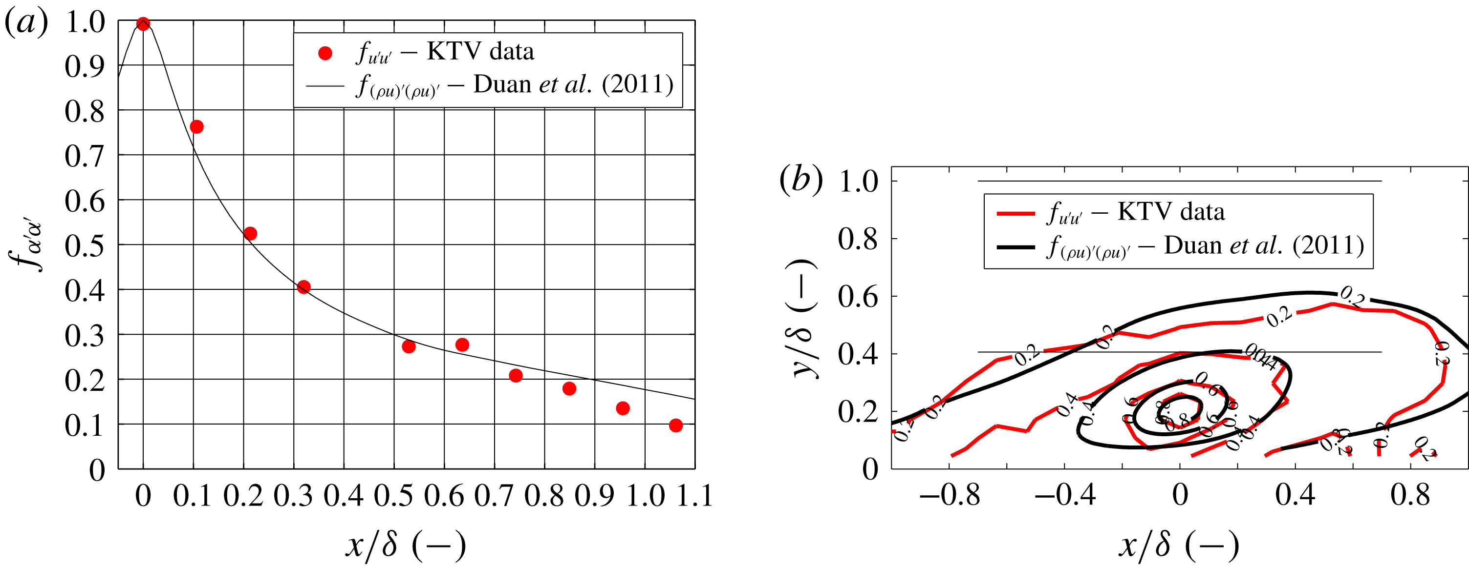
from Duan, Beekman & Martin (Reference Duan, Beekman and Martin2011). (b) Contours of correlation. Thin horizontal lines mark the boundary-layer edge and approximate wake-region boundary. KTV data in red, DNS data in black.

With the ability to write multiple lines, the longitudinal correlation coefficient can be calculated as
 $$\begin{eqnarray}f(\boldsymbol{x},r)=\frac{\overline{u^{\prime }(\boldsymbol{x})u^{\prime }(\boldsymbol{x}+r)}}{\overline{u^{\prime 2}}}=\frac{R_{u^{\prime }u^{\prime }}}{\overline{u^{\prime 2}}}\end{eqnarray}$$
by using the spacing between each write line,
 $r$
. The longitudinal correlation of the streamwise-velocity data is presented in figure 7(a) for
 $y/\unicode[STIX]{x1D6FF}\approx 0.2$
. As a means of first comparison,
 $f_{u^{\prime }u^{\prime }}$
from the present KTV boundary-layer data is compared to
 $f_{(\unicode[STIX]{x1D70C}u)^{\prime }(\unicode[STIX]{x1D70C}u)^{\prime }}$
from Duan et al. (Reference Duan, Beekman and Martin2011). It should be noted that the work from Duan et al. (Reference Duan, Beekman and Martin2011) is at different conditions,
 $M_{\infty }=2.97$
,
 $Re_{\unicode[STIX]{x1D6E9}}=3030$
.
Sample instantaneous shock-wave/turbulent boundary-layer interaction fluorescence exposures for the (a)
 $8^{\circ }$
, (b)
 $16^{\circ }$
, (c)
 $24^{\circ }$
and (d)
 $32^{\circ }$
corners, respectively. These are ostensibly boundary-layer profiles traces with a 500 ns prescribed delay between the write and read steps. Major tick marks are 10 mm. Flow is left to right. Inverted intensity scale. Wall marked as black. Animations of instantaneous fluorescence exposures and corresponding velocity profiles are provided in the supplementary material (movie 1, movie 2, movie 3 and movie 4 for the 8, 16, 24 and 32 degree corners, respectively).

Moreover, because the flow field should have forward and backward symmetry, the number of points used for the longitudinal correlation can be increased from 10 to 19 by performing the correlation in (4.4) from left-to-right and also right-to-left and concatenating the datasets. This correlation is performed for the field recorded in figure 5 for
 $y/\unicode[STIX]{x1D6FF}\approx 0.2$
and presented in figure 7(b). Thin horizontal lines in figure 7(b) mark the boundary-layer edge at
 $y/\unicode[STIX]{x1D6FF}=1$
and also the approximate location of the wake-region boundary at
 $y/\unicode[STIX]{x1D6FF}\approx 0.41$
. Contours of
 $f_{(\unicode[STIX]{x1D70C}u)^{\prime }(\unicode[STIX]{x1D70C}u)^{\prime }}$
as computed by DNS data from Duan et al. (Reference Duan, Beekman and Martin2011) are plotted in black, and contours of
 $f_{u^{\prime }u^{\prime }}$
as measured from KTV data are plotted in red. The KTV data have more scatter, as expected, but the orientation of the contours is quite similar, indicating that the average angle of turbulent structures is also similar.
In this section, KTV data were compared to those in the literature for a supersonic turbulent boundary layer. From this, we conclude that the nature of the incoming flow can be considered a nominal supersonic turbulent boundary layer enabling the study of shock-wave/turbulent boundary-layer interaction.
5 Shock-wave/turbulent boundary-layer interaction results
In this section, we present the results from experiments designed to investigate turbulent, supersonic corner flows at four different angles:
 $8^{\circ }$
,
 $16^{\circ }$
,
 $24^{\circ }$
and
 $32^{\circ }$
. This is done by fixing a wedge of the appropriate geometry in Port 2 of the M3CT (see figure 1). The root of the corner flow (
 $x/\unicode[STIX]{x1D6FF}=0$
) is placed near the centre of the boundary-layer measurement location presented in § 4.
Figure 8 shows sample KTV read exposures for each case. This is the visualization of the
 $5p[3/2]_{1}\rightarrow 5s[3/2]_{1}^{o}$
(829.8 nm) transition. Mach 2.8 flow is left to right and the walls in each corner flow are marked in black. These data are reduced by following the same procedure as in § 4 for tracing the profiles in the write and read images. Animations of instantaneous fluorescence exposures and corresponding velocity profiles are provided as in the supplementary material (movie 1, movie 2, movie 3 and movie 4 for the 8, 16, 24 and 32 degree corners, respectively), available online at https://doi.org/10.1017/jfm.2018.1029.
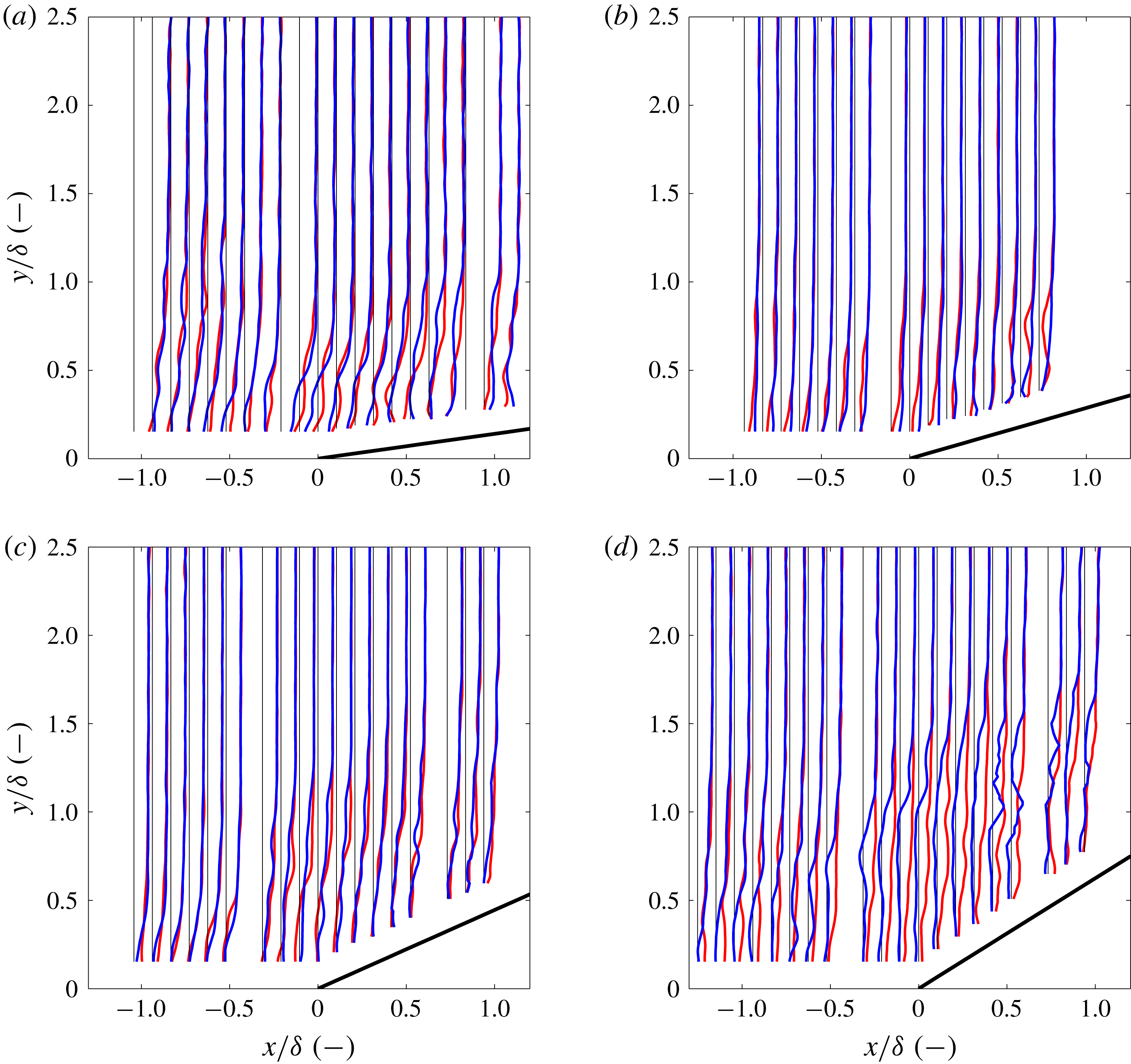
Examples of non-dimensional instantaneous velocity profiles (
 $u/(12U_{\infty })$
) are presented in figure 9. For each corner angle, we show the write location marked as a thin, vertical black line and two randomly selected, example instantaneous velocity profiles in blue and red. This is intended to visualize relative unsteadiness of each corner flow. Results are not presented within
 $y/\unicode[STIX]{x1D6FF}<0.1$
because the signal to noise ratio was too low to provide data with high confidence. In addition, there is a missing velocity profile every 10 mm because there is a gap between the microlens arrays that yields insufficient focusing and thus low SNR.
Sample non-dimensional (
 $u/(12U_{\infty })$
), instantaneous shock-wave/turbulent boundary-layer interaction velocity profiles represented in blue and red for the (a)
 $8^{\circ }$
, (b)
 $16^{\circ }$
, (c)
 $24^{\circ }$
and (d)
 $32^{\circ }$
corners, respectively. Thin vertical black line represents the write location. Flow is left to right.

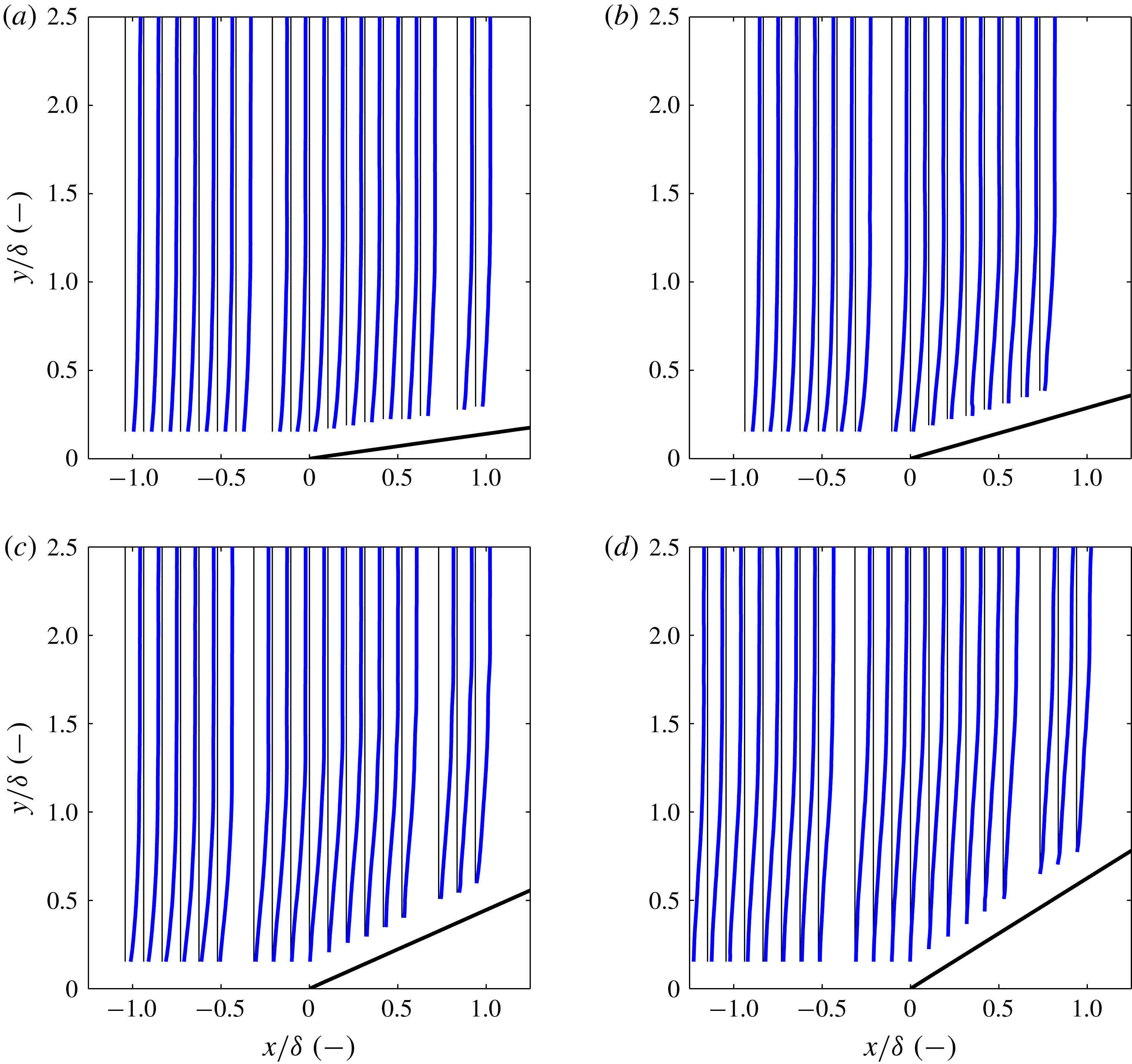
In figure 10, we present non-dimensional mean-velocity profiles (
 $u/(12U_{\infty })$
). For each corner angle, we show the write location marked as a thin, vertical black line and the mean-velocity profile as a thicker blue line. In the
 $8^{\circ }$
and
 $16^{\circ }$
cases, there are no clearly apparent points of inflection in the mean profiles. In the
 $24^{\circ }$
case, near to the root (
 $-0.5\lesssim x/\unicode[STIX]{x1D6FF}\lesssim 0.5$
), and to a much greater extent in the
 $32^{\circ }$
case (the field of view), there appear to be clear points of inflection in the mean boundary-layer profiles.
Non-dimensional (
 $u/(12U_{\infty })$
), mean shock-wave/turbulent boundary-layer interaction velocity profiles for the (a)
 $8^{\circ }$
, (b)
 $16^{\circ }$
, (c)
 $24^{\circ }$
and (d)
 $32^{\circ }$
corners, respectively. Thin vertical black line represents the write location. Flow is left to right. Error bars are not plotted because they are not visible at the present scale. We estimate the uncertainty as 5 % in the free stream and 15 % near the wall.

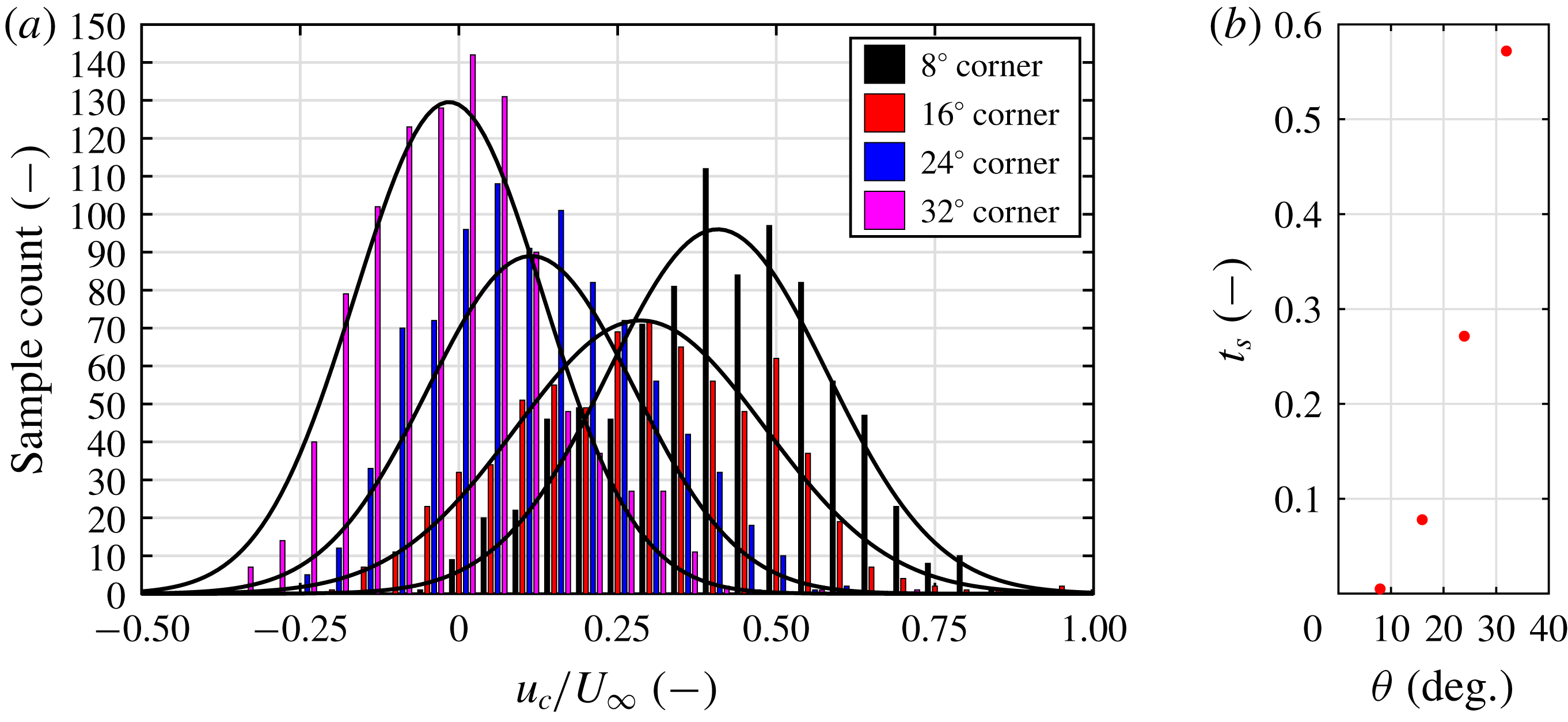
In figure 11(a) we show the distribution of the instantaneous normalized velocity at the root (
 $u_{c}/U_{\infty }$
) for all corner angles. We define a parameter to quantify the flow separation as
 $t_{s}=C_{s}/C_{T}$
, where
 $C_{s}$
is the number of counts (or snapshots) in which
 $u_{c}<0$
and
 $C_{T}$
is the total number of counts. This represents the percentage of the total snapshots in which the flow near the root is separated. It is observed that for the
 $8^{\circ }$
case, the flow for all practical purposes is not separated. Beginning with the
 $16^{\circ }$
case, the mean of the velocity shifts to the left as separation becomes more prominent. We also show the scaling of
 $t_{s}$
with wedge angle in figure 11(b).
(a) Distribution of normalized velocity (
 $u_{c}/U_{\infty }$
) near the root for all wedge angles. (b) Scaling of
 $t_{s}$
with corner angle
 $\unicode[STIX]{x1D703}$
.

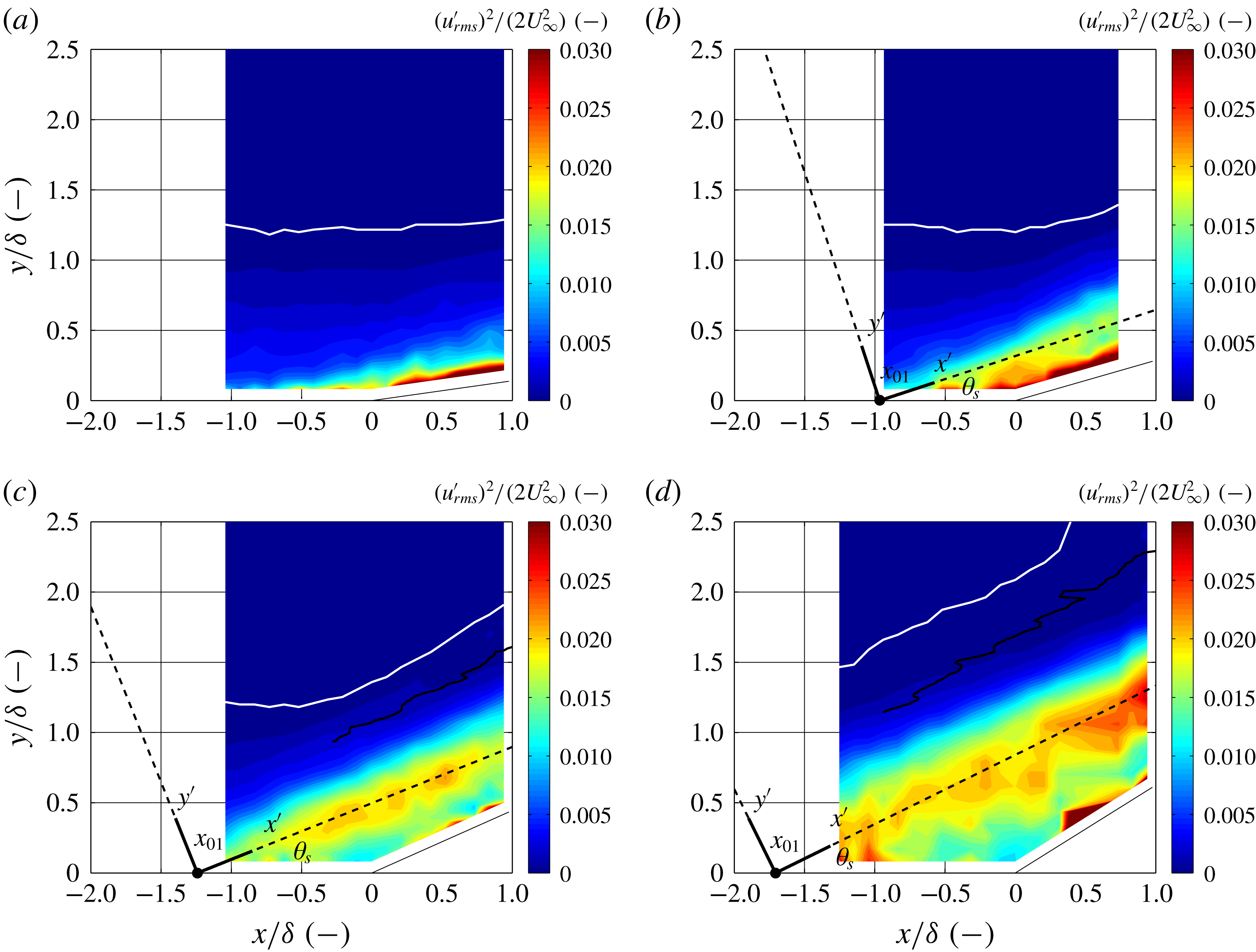
Contours of the streamwise component of turbulent kinetic energy (sTKE),
 $(u_{rms}^{\prime })^{2}/(2U_{\infty }^{2})$
, are presented in figure 12. For each case, very close to the wall on the ramp, there is a notable increase in fluctuations. This is most likely an artefact of the residual noise from the KTV read step. Despite this, in the
 $16^{\circ }$
,
 $24^{\circ }$
and
 $32^{\circ }$
cases, a shear layer can clearly be identified as a maximum in fluctuations along a ray inclined at an angle similar to that of the corner angle. No such shear layer was observed in the
 $8^{\circ }$
case. Also superimposed on the contour plots is a white demarcation line denoting the points where
 $u_{rms}^{\prime }=0.02U_{\infty }$
, i.e. when the turbulence intensity reaches the level of the noise in the tunnel.
Contours of the non-dimensional streamwise turbulent kinetic energy (sTKE)
 $(u_{rms}^{\prime })^{2}/(2U_{\infty }^{2})$
) for the (a)
 $8^{\circ }$
, (b)
 $16^{\circ }$
, (c)
 $24^{\circ }$
and (d)
 $32^{\circ }$
corners, respectively. The shear-layer coordinate system fitted to the maximum sTKE is overlaid. Flow is left to right. Mean shock position shown in black. White line marks
 $y_{u}/\unicode[STIX]{x1D6FF}$
which is the wall-normal location above which the streamwise-velocity fluctuations are less than 2 % of the free-stream velocity, or
 $u_{rms}^{\prime }=0.02U_{\infty }$
.

To characterize the shear layers, two parameters were determined:
 $\unicode[STIX]{x1D703}_{s}$
, which is the angle of the shear-layer coordinate system (
 $x^{\prime }$
,
 $y^{\prime }$
) relative to the laboratory coordinate system (
 $x$
,
 $y$
), and
 $x_{01}$
, which is the origin of the (
 $x^{\prime }$
,
 $y^{\prime }$
) coordinate system. The parameters were found by fitting an equation of the form
 $y=\tan \unicode[STIX]{x1D703}_{s}(x-x_{01})$
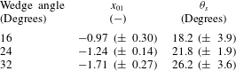
to the spatial locations of the maximum sTKE at each streamwise location. The results for the corners are overlaid on the sTKE contours in figure 12 and the values for
 $\unicode[STIX]{x1D703}_{s}$
and
 $x_{01}$
are given in table 2. In performing this analysis it is assumed that the sTKE (
 $u^{\prime 2}/(2U_{\infty }^{2})$
) is an acceptable surrogate for the total TKE
 $((u^{\prime 2}+v^{\prime 2}+w^{\prime 2})/(2U_{\infty }^{2}))$
.
Shear-layer origin,
 $x_{01}$
, and angle
 $\unicode[STIX]{x1D703}_{s}$
. Uncertainties estimated as the 95 % confidence intervals in the linear fits.

In Helm, Martin & Dupont (Reference Helm, Martin and Dupont2014), the researchers show that the shear layer over a
 $24^{\circ }$
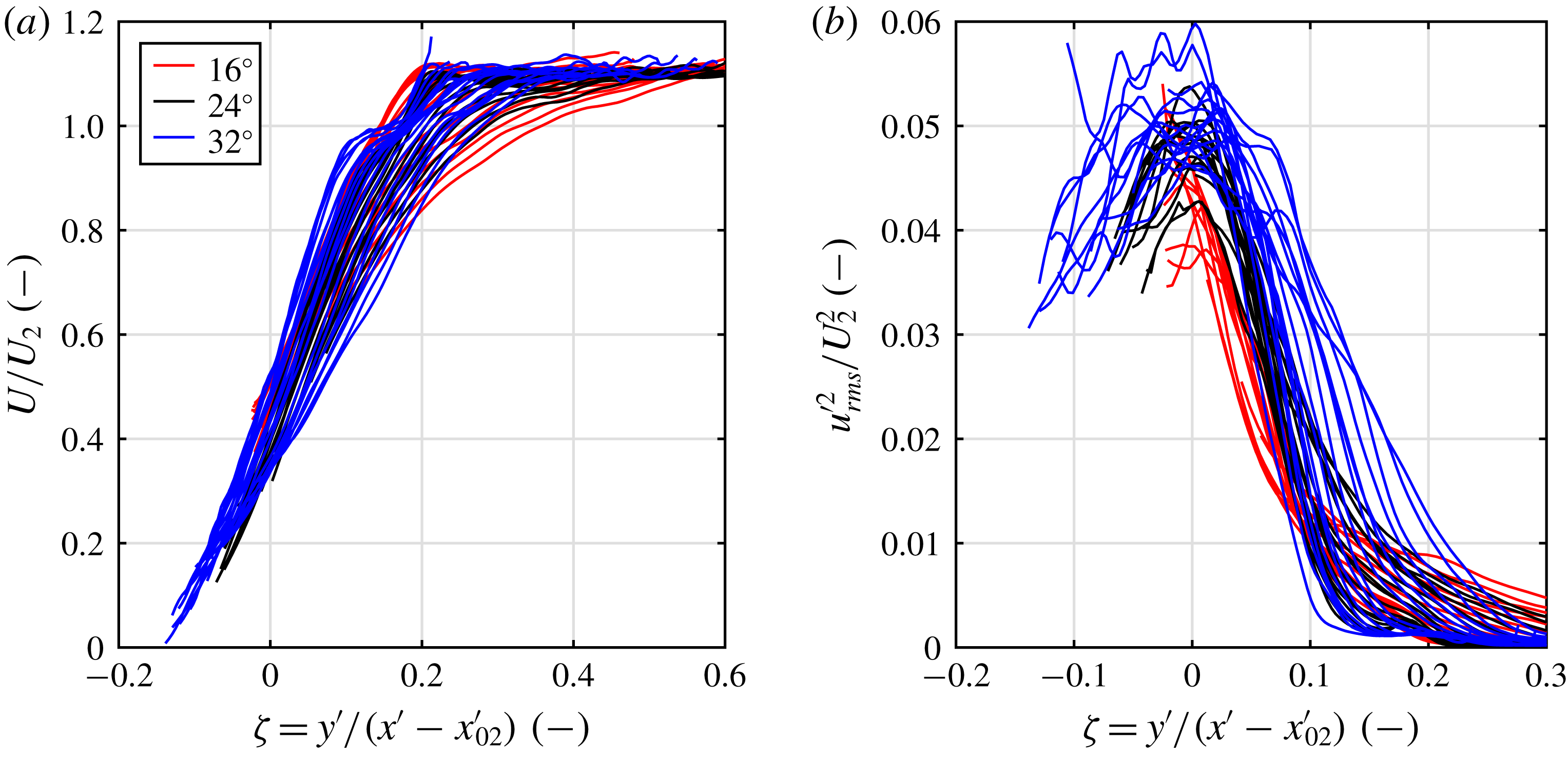
corner may be collapsed in a self-similar fashion. They apply a coordinate transformation to the two-dimensional velocity calculations in the laboratory frame to determine the velocity in the shear-layer coordinate system. Unfortunately, in this work a rotation may not be applied as the KTV measurements were one-dimensional. Despite this, we use the velocity in the laboratory frame as a surrogate for the velocity in the shear-layer coordinate system and attempt to identify self-similarity to first approximation. In figure 13, we attempt to collapse the
 $U/U_{2}$
and
 $u_{rms}^{\prime 2}/U_{2}^{2}$
profiles to a single curve, where
 $U$
is the mean velocity and
 $U_{2}$
is the velocity downstream of the shock as calculated by the inviscid flow relations for the measured shock angle. The similarity variable used is
 $\unicode[STIX]{x1D701}=y^{\prime }/(x^{\prime }-x_{02}^{\prime })$
, where
 $x_{02}$
is the imaginary origin of the shear layer, which is computed by iterating until the profiles collapse. It should be noted that unlike in Helm et al. (Reference Helm, Martin and Dupont2014),
 $u_{rms}^{\prime }$
is the
 $x$
component of the fluctuating velocity in the (
 $x$
,
 $y$
) coordinate system, not the
 $x^{\prime }$
component of the fluctuating velocity in the (
 $x^{\prime }$
,
 $y^{\prime }$
) coordinate system. Compared to Helm et al. (Reference Helm, Martin and Dupont2014), figure 13 shows more scatter and the collapse is not qualitatively as good. Despite this and the limitations in the analysis, self-similar behaviour is apparent to a first approximation.
(a) The
 $U/U_{2}$
profiles plotted against the similarity variable
 $\unicode[STIX]{x1D701}$
for the
 $16^{\circ }$
,
 $24^{\circ }$
and
 $32^{\circ }$
corners. (b) The
 $u_{rms}^{\prime 2}/U_{2}^{2}$
profiles plotted against the similarity variable
 $\unicode[STIX]{x1D701}$
for the
 $16^{\circ }$
,
 $24^{\circ }$
and
 $32^{\circ }$
corners. Here,
 $U_{2}$
is the downstream velocity as calculated from oblique shock relations for a Mach 2.8 flow and the shock angle as measured form the schlieren images.

6 Wall-normal integrated streamwise turbulent kinetic energy
In this section, we present an analysis of the sTKE (
 $u_{rms}^{\prime 2}/2$
) in profile form (as opposed to the contours presented earlier) to identify trends in sTKE with compression-corner angle. We define a figure of merit as the wall-normal integrated sTKE at a particular streamwise location as
 $$\begin{eqnarray}\overline{\text{sTKE}}=\int _{y_{l}/\unicode[STIX]{x1D6FF}}^{y_{u}/\unicode[STIX]{x1D6FF}}\frac{u_{rms}^{\prime 2}}{2U_{\infty }^{2}}\,\text{d}\left(\frac{y}{\unicode[STIX]{x1D6FF}}\right),\end{eqnarray}$$
where the lower limit,
 $y_{l}/\unicode[STIX]{x1D6FF}$
, is the lowest wall-normal location where KTV data were collected, and the upper integration limit,
 $y_{u}/\unicode[STIX]{x1D6FF}$
, is the wall-normal location above which the streamwise velocity fluctuations are less than 2 % of the free-stream velocity, or
 $u_{rms}^{\prime }=0.02U_{\infty }$
. A threshold of 2 % was chosen because it is just above the measured free-stream streamwise-velocity-fluctuation level in this wind tunnel, which is 1.0–1.5 %. The threshold,
 $y_{u}/\unicode[STIX]{x1D6FF}$
, is presented as a white line in the TKE contours in figure 12. As such, we isolate the streamwise fluctuations in the boundary layer and the shock-wave/boundary-layer interaction from those in the wind tunnel free stream and the measurement noise. We note that the
 $\overline{\text{sTKE}}$
results presented herein are relatively insensitive to the choice of this threshold in the range of 1.5–4.0 %.
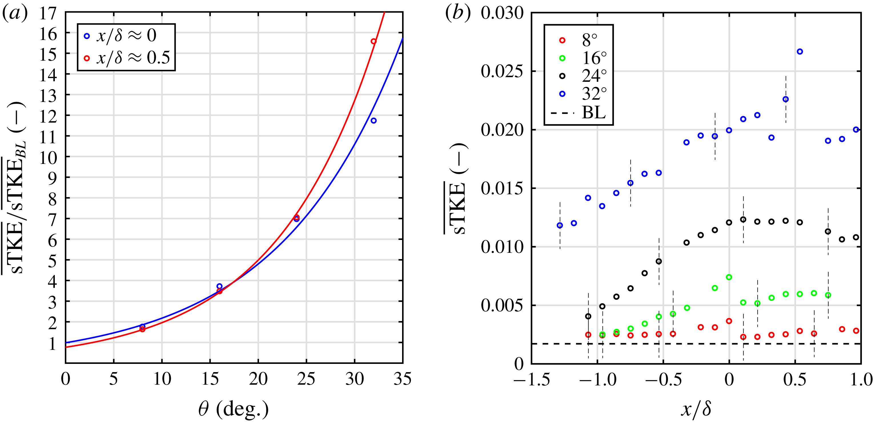
Ultimately, this figure of merit is designed to identify turbulence amplification by accounting for both the amplitude of the velocity fluctuations and shear-layer width for the different geometries. In figure 14(a) we present the
 $\overline{\text{sTKE}}$
for each streamwise location. It is observed that
 $\overline{\text{sTKE}}$
increases with increasing
 $x/\unicode[STIX]{x1D6FF}$
. In figure 14(b),
 $\overline{\text{sTKE}}$
is plotted against the corner angle at locations downstream of and at the corner. We normalize by the
 $\overline{\text{sTKE}}$
in the boundary layer (figure 6
b) to find the effect of compression-corner angle on wall-normal integrated streamwise turbulence amplification. The trend of
 $\overline{\text{sTKE}}$
with compression-corner angle is found to be an exponential. The parameters for this scaling are given in table 3 for the two locations. Sensibly, the coefficients of the exponentials in table 3 are close to unity (within experimental error) which implies no amplification at zero compression-corner angle.
Sclaing relations for
 $\overline{\text{sTKE}}$
.

(a) Variation of
 $\overline{\text{sTKE}}$
along the streamwise direction for
 $8^{\circ }$
,
 $16^{\circ }$
,
 $24^{\circ }$
and
 $32^{\circ }$
corners. Error bars shown as vertical dashed lines. (b) Scaling of
 $\overline{\text{sTKE}}$
with wedge angle for locations at and downstream of the root, where the values at
 $x/\unicode[STIX]{x1D6FF}\approx 0$
are the averages of the points adjacent to and at the root.

7 Proper orthogonal decomposition
The proper orthogonal decomposition (POD) technique can be used to extract spatial and temporal structures from a turbulent flow field (Lumley Reference Lumley, Yaglom and Tatarsky1967; Berkooz et al. Reference Berkooz, Holmes and Lumley1993; Taira et al. Reference Taira, Brunton, Dawson, Rowley, Colonius, McKeon, Schmidt, Gordeyev, Theofilis and Ukeiley2017). This approach decomposes the original vector or scalar field into a weighted, linear sum of basis functions, or modes. In the present work, the instantaneous streamwise-velocity fields are recorded at 10 Hz so they are nominally uncorrelated in time; thus, the snapshot method of Sirovich (Reference Sirovich1987) was chosen to analyse the data.
Following the terminology in Sirovich (Reference Sirovich1987) and Stöhr, Sadanandan & Meier (Reference Stöhr, Sadanandan and Meier2011), the streamwise-velocity fields are decomposed into a mean and fluctuating component as
 $$\begin{eqnarray}u_{i}(x,y)=\overline{u}(x,y)+u_{i}^{\prime }(x,y).\end{eqnarray}$$
In the datasets presented here, there are
 $p$
points in the streamwise direction and
 $q$
points in the wall-normal direction (
 $M=p\times q$
total grid points) with
 $N$
number of snapshots (
 $i=1\ldots N$
). The fluctuating streamwise-velocity field,
 $u_{i}^{\prime }(x,y)$
, is reshaped into a matrix,
 $\unicode[STIX]{x1D650}^{\prime }$
, with elements
 $U_{i}^{\prime }(X_{n})$
where the
 $n=1\ldots M$
points for each snapshot form a row for
 $i=1\ldots N$
rows, so
 $\unicode[STIX]{x1D650}^{\prime }$
is of dimensions
 $N\times M$
and can be written as
 $$\begin{eqnarray}\unicode[STIX]{x1D650}^{\prime }=\left[\begin{array}{@{}cccc@{}}u_{1}^{\prime }(x_{1},y_{1}) & u_{1}^{\prime }(x_{2},y_{1}) & .. & u_{1}^{\prime }(x_{p},y_{q})\\ u_{2}^{\prime }(x_{1},y_{1}) & u_{2}^{\prime }(x_{2},y_{1}) & .. & u_{2}^{\prime }(x_{p},y_{q})\\ : & : & .. & :\\ : & : & .. & :\\ u_{N}^{\prime }(x_{1},y_{1}) & u_{N}^{\prime }(x_{2},y_{1}) & .. & u_{N}^{\prime }(x_{p},y_{q})\end{array}\right]=\left[\begin{array}{@{}cccc@{}}U_{1}^{\prime }(X_{1}) & U_{1}^{\prime }(X_{2}) & ... & U_{1}^{\prime }(X_{M})\\ U_{2}^{\prime }(X_{1}) & U_{2}^{\prime }(X_{2}) & ... & U_{2}^{\prime }(X_{M})\\ : & : & ... & :\\ : & : & ... & :\\ U_{N}^{\prime }(X_{1}) & U_{N}^{\prime }(X_{2}) & ... & U_{N}^{\prime }(X_{M})\end{array}\right].\end{eqnarray}$$
Where
 $U_{1}^{\prime }(X_{2})$
is the value of
 $u^{\prime }$
at the spatial location
 $X_{2}$
in the 1st snapshot and so on. We assume that the velocity may be written as
 $$\begin{eqnarray}U_{i}^{\prime }(X_{n})=\mathop{\sum }_{j=1}^{N}a_{ij}\unicode[STIX]{x1D719}_{j}(X_{n}).\end{eqnarray}$$
Here,
 $\unicode[STIX]{x1D719}_{j}(X_{n})$
is the
 $j$
th eigenfunction (or mode) and
 $a_{ij}$
is the coefficient of the
 $j$
th mode that corresponds to the
 $i$
th snapshot of the velocity field. The goal is to prescribe a condition that would allow us to identify flow structures within a mode
 $\unicode[STIX]{x1D719}_{j}$
. The condition that achieves this, following Berkooz et al. (Reference Berkooz, Holmes and Lumley1993), is that the decomposition be optimal. Optimal here means that for a given number of modes, the decomposition will contain the most kinetic energy possible out of all possible decompositions. When this condition is met, the decomposition in (7.3) will represent the proper orthogonal decomposition. To impose the optimality condition, the Fredholm integral eigenvalue problem must be solved,
 $$\begin{eqnarray}\int _{\unicode[STIX]{x1D6FA}}R(X_{m},X_{n})\unicode[STIX]{x1D719}_{j}(X_{n})\,\text{d}\unicode[STIX]{x1D6FA}=\overline{\unicode[STIX]{x1D706}}\unicode[STIX]{x1D719}_{j}(X_{m}).\end{eqnarray}$$
Here,
 $m$
is a free index (
 $m=1\ldots M$
),
 $\overline{\unicode[STIX]{x1D706}}$
is the eigenvalue of mode
 $j$
and
 $\unicode[STIX]{x1D6FA}$
is the region of integration, which is the flow field space.
 $R(X_{m},X_{n})$
is the two-point correlation defined as,
 $$\begin{eqnarray}R(X_{m},X_{n})=\overline{U^{\prime }(X_{m})U^{\prime }(X_{n})}.\end{eqnarray}$$
To solve the eigenvalue problem, the integral in (7.4) must be approximated by a finite sum. This is accomplished by writing
 $$\begin{eqnarray}\mathop{\sum }_{n=1}^{M}R(X_{m},X_{n})\unicode[STIX]{x1D719}_{j}(X_{n})\unicode[STIX]{x0394}\unicode[STIX]{x1D6FA}_{n}=\overline{\unicode[STIX]{x1D706}}\unicode[STIX]{x1D719}_{j}(X_{m}).\end{eqnarray}$$
Here, we have divided the domain into
 $M$
subdivisions, each of size
 $\unicode[STIX]{x0394}\unicode[STIX]{x1D6FA}_{n}$
. Each subdivision encompasses a spatial (measurement) location
 $X_{n}$
. To solve the eigenvalue problem in MATLAB, the matrix
 $\unicode[STIX]{x1D64D}$
, whose elements are
 $R(X_{m},X_{n})$
, can be constructed from
 $\unicode[STIX]{x1D650}^{\prime }$
as,
 $$\begin{eqnarray}\unicode[STIX]{x1D64D}=\frac{1}{N}\unicode[STIX]{x1D650}^{\prime T}\unicode[STIX]{x1D650}^{\prime }\end{eqnarray}$$
where the superscript
 $T$
denotes the matrix transpose. The dimensions of
 $\unicode[STIX]{x1D64D}$
are
 $M\times M$
. Using this, the eigenvalue problem of (7.6) can be written as,
 $$\begin{eqnarray}\unicode[STIX]{x1D64D}\overline{\unicode[STIX]{x1D652}}\unicode[STIX]{x1D753}_{\boldsymbol{j}}=\overline{\unicode[STIX]{x1D706}}\unicode[STIX]{x1D753}_{\boldsymbol{j}}.\end{eqnarray}$$
Here
 $\overline{\unicode[STIX]{x1D652}}$
is a diagonal matrix of dimensions
 $M\times M$
which contains the
 $\unicode[STIX]{x0394}\unicode[STIX]{x1D6FA}_{n}$
values for all the spatial locations and
 $\unicode[STIX]{x1D753}_{\boldsymbol{j}}$
is a
 $M\times 1$
column vector whose elements are
 $\unicode[STIX]{x1D719}_{j}(X_{n})$
(
 $n=1\ldots M$
). From
 $\overline{\unicode[STIX]{x1D652}}$
can extract a constant
 $\unicode[STIX]{x0394}\unicode[STIX]{x1D6FA}$
and can write the eigenvalue problem as,
 $$\begin{eqnarray}\unicode[STIX]{x0394}\unicode[STIX]{x1D6FA}\unicode[STIX]{x1D64D}\unicode[STIX]{x1D652}\unicode[STIX]{x1D753}_{\boldsymbol{j}}=\overline{\unicode[STIX]{x1D706}}\unicode[STIX]{x1D753}_{\boldsymbol{j}}.\end{eqnarray}$$
Now
 $\unicode[STIX]{x1D652}$
contains the spatial weights of each location relative to the constant
 $\unicode[STIX]{x0394}\unicode[STIX]{x1D6FA}$
and has no units. Furthermore, we can combine
 $\unicode[STIX]{x0394}\unicode[STIX]{x1D6FA}$
with the eigenvalue (
 $\unicode[STIX]{x1D706}=\overline{\unicode[STIX]{x1D706}}/\unicode[STIX]{x0394}\unicode[STIX]{x1D6FA}$
) to write,
 $$\begin{eqnarray}\unicode[STIX]{x1D64D}\unicode[STIX]{x1D652}\unicode[STIX]{x1D753}_{\boldsymbol{j}}=\unicode[STIX]{x1D706}\unicode[STIX]{x1D753}_{\boldsymbol{j}}.\end{eqnarray}$$
Note that the eigenvalue
 $\unicode[STIX]{x1D706}$
has units of
 $\text{m}^{2}~\text{s}^{-2}$
in this work. Equation (7.10) represents the general eigenvalue problem and can be solved once
 $\unicode[STIX]{x1D652}$
is determined. In the case of this work, the laser lines are evenly spaced except at two locations in the flow field. These locations correspond to the missing velocity profiles because of the gap in the microlens array. Therefore the spatial points in the two laser lines adjacent to the missing line have to be weighted by a factor of 1.5 more than all the other points in order to integrate over the entire domain. However it was found that, by neglecting or adding the different spatial weights of the aforementioned points, the changes in the results were negligible, therefore in this work
 $\unicode[STIX]{x1D652}$
was the identity matrix and the eigenvalue problem further simplifies to,
 $$\begin{eqnarray}\unicode[STIX]{x1D64D}\unicode[STIX]{x1D753}_{\boldsymbol{j}}=\unicode[STIX]{x1D706}\unicode[STIX]{x1D753}_{\boldsymbol{j}}.\end{eqnarray}$$
The dimensions of
 $\unicode[STIX]{x1D64D}$
are
 $M\times M$
, which in this work are
 ${\approx}2500\times 2500$
. This a fairly large matrix whose eigenvalue computation is expensive. To address this computational cost, Sirovich (Reference Sirovich1987) suggested solving the following nominally equivalent eigenvalue problem,
 $$\begin{eqnarray}\unicode[STIX]{x1D63E}\boldsymbol{e}_{\boldsymbol{j}}=\unicode[STIX]{x1D706}\boldsymbol{e}_{\boldsymbol{j}}.\end{eqnarray}$$
Where
 $\unicode[STIX]{x1D63E}=(1/N)\unicode[STIX]{x1D650}^{\prime }\unicode[STIX]{x1D650}^{\prime T}$
, with dimensions of
 $N\times N$
and
 $\boldsymbol{e}_{\boldsymbol{j}}$
is the eigenfunction (represented here as a column vector). In this work
 $N\approx 900$
and therefore (7.12) is less computationally expensive than (7.11). The POD modes can be derived from (7.12) as (Stöhr et al.
Reference Stöhr, Sadanandan and Meier2011),
 $$\begin{eqnarray}\unicode[STIX]{x1D719}_{j}(X_{n})=\frac{1}{\unicode[STIX]{x1D706}_{j}N}\mathop{\sum }_{i=1}^{N}a_{ij}U_{i}^{\prime }(X_{n}).\end{eqnarray}$$
The mode coefficients
 $a_{ij}$
are,
 $$\begin{eqnarray}a_{ij}=e_{ij}\sqrt{\unicode[STIX]{x1D706}_{j}N}.\end{eqnarray}$$
The POD modes form an orthonormal set and are normalized such that,
 $$\begin{eqnarray}\unicode[STIX]{x1D753}_{\boldsymbol{i}}\boldsymbol{\cdot }\unicode[STIX]{x1D753}_{\boldsymbol{j}}=\unicode[STIX]{x1D6FF}_{ij},\end{eqnarray}$$
where
 $\unicode[STIX]{x1D6FF}_{ij}$
is the Kronecker delta and ‘
 $\boldsymbol{\cdot }$
’ denotes the vector dot product. The eigenvalues have special significance because,
 $$\begin{eqnarray}E_{tot}=\mathop{\sum }_{n=1}^{M}\overline{R(X_{n},X_{n})}=\mathop{\sum }_{j=1}^{N}\unicode[STIX]{x1D706}_{j}.\end{eqnarray}$$
Consequently, each eigenvalue represents the contribution of its corresponding mode to the total energy, and in the discussion of results, the energies (
 $\unicode[STIX]{x1D706}_{j}$
), will be normalized by this
 $E_{tot}$
.
It should be noted that in the preceding formulation, thermodynamic variables are not considered because none were measured in these experiments. Sirovich (Reference Sirovich1987) and Rowley, Colonius & Murray (Reference Rowley, Colonius and Murray2004) state that in a compressible flow, both the velocity and thermodynamic variables are dynamically important and should be included in the analysis. In this work, only the streamwise-velocity fluctuations are measured and so the analysis is limited in this sense. However, researchers have used POD of single components of velocity to successfully examine the structure of compressible turbulent flows. For example, Murray et al. (Reference Murray, Sällström and Ukeiley2009) used the vertical component of velocity to study the structure of subsonic open cavities. To estimate the effect of a compressible flow field to a first approximation, the density field is broken into pre- and post-shock values. The first value is the value in the free stream and the second is calculated from the oblique shock relations with the shock position serving as a demarcation line. Then, POD analysis is carried out for
 $\sqrt{\unicode[STIX]{x1D70C}}u^{\prime }$
(instead of
 $u^{\prime }$
), which results in eigenvalues that are representative of
 $\unicode[STIX]{x1D70C}u^{\prime 2}$
, which is the turbulent kinetic energy. However, we observed that this correction did not significantly alter the structure and spectrum of the POD modes for these experiments; hence, the formulation without the density was used.
8 Eigenvalues of snapshot POD analysis
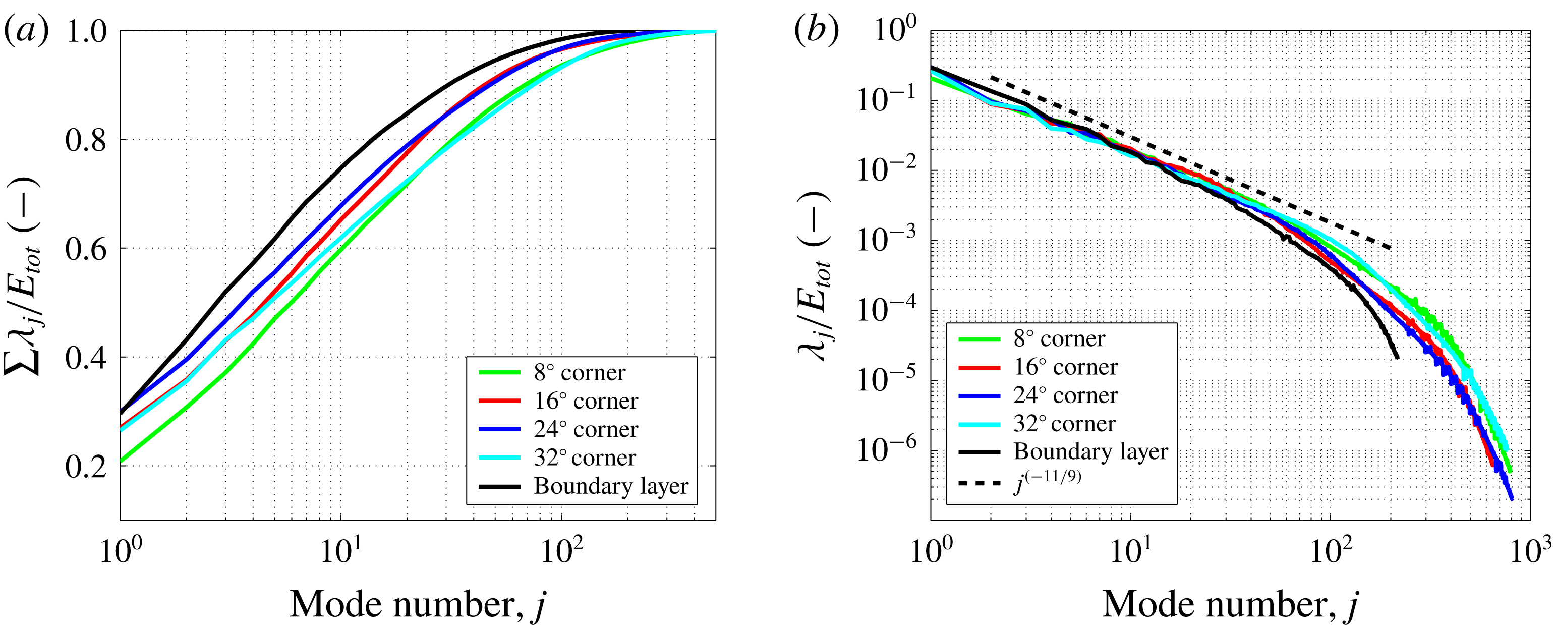
In this section, we present and discuss the eigenvalue results from applying the snapshot POD method to the KTV data reported in earlier sections. In figure 15(a), we present the cumulative fractional energy versus mode number. For each case, the first mode accounts for
 ${\approx}20{-}30\,\%$
of the
 $E_{tot}$
(7.16) and the first 6–10 modes capture approximately 60 % of the
 $E_{tot}$
in the flow. No clear trends as to the fraction of energy of the first mode or the cumulative fractional energy can be found between the different flow fields investigated in this work.
The eigenvalue spectrum is plotted for each case in figure 15(b). Knight & Sirovich (Reference Knight and Sirovich1990) and Moser (Reference Moser1994) suggest that the POD eigenfunctions are a good set of basis functions with which to form an inertial-range spectrum for inhomogeneous, turbulent flows, as is the case here. The famous inertial-range scaling due to Kolmogorov (Kolmogorov Reference Kolmogorov1941) is
 $$\begin{eqnarray}E\propto \unicode[STIX]{x1D716}^{2/3}k^{-5/3},\end{eqnarray}$$
where
 $E$
is the energy per scalar wavenumber,
 $\unicode[STIX]{x1D716}$
is the dissipation rate and
 $k$
is the wavenumber. Stated equivalently
 $$\begin{eqnarray}{\mathcal{E}}\propto \unicode[STIX]{x1D716}^{2/3}k^{-11/3},\end{eqnarray}$$
where
 ${\mathcal{E}}$
is the energy per vector wavenumber. Knight & Sirovich (Reference Knight and Sirovich1990) argue that the wavenumber is proportional to the mode number as
 $k\propto j^{1/3}$
, and so in the inertial range the eigenvalues scale as
 $$\begin{eqnarray}\unicode[STIX]{x1D706}_{j}\propto j^{-11/9},\end{eqnarray}$$
which is represented in figure 15(b) as a dashed line. Knight & Sirovich (Reference Knight and Sirovich1990) also state that the inertial range will be shorter by a factor of three in equivalent wavenumber space (measured in decades). The differences between the different spectra presented here are modest for mode numbers
 $j<100$
, above which the noise from the measurement technique may play a role.
The authors initially expected an appreciably different eigenvalue spectrum when comparing each case because of how dissimilar and inhomogeneous the flow fields are. For example, the
 $32^{\circ }$
corner flow is inhomogeneous in the streamwise and wall-normal directions and has a relatively large separated region. This is in contrast to the boundary-layer flow, which is attached and inhomogeneous in only the wall-normal direction, yet the spectra are similar. However, upon close inspection, the first few POD modes do not clearly scale as
 $j^{-11/9}$
, and these modes contain the structures (inhomogeneity and separation) which strongly modify the mean flow; this will be evident in the forthcoming presentation of the POD modes.
(a) The cumulative fraction of energy,
 $\sum \unicode[STIX]{x1D706}_{j}/E_{tot}$
. (b) The fraction of energy of each mode,
 $\unicode[STIX]{x1D706}_{j}/E_{tot}$
. The black line is the mode number raised to the (
 $-11/9$
) power as suggested by Knight and Sirovitch (Knight & Sirovich Reference Knight and Sirovich1990).

This scaling of the eigenvalues is similar to that found in Piponniau et al. (Reference Piponniau, Collin, Dupont and Debiève2012) where a POD analysis was performed on PIV results from an induced-shock-wave/turbulent boundary-layer interaction. Piponniau et al. (Reference Piponniau, Collin, Dupont and Debiève2012) report a smaller observed value of the roll off (
 $\unicode[STIX]{x1D706}\propto j^{-0.9}$
) which may be due to the fact that: (i) the flow field is not the same (impinged-shock/boundary-layer interaction versus corner flow); (ii) it is understood that the wall-normal component of the fluctuating velocity tends to have a flatter spectrum in high-speed wall-bounded boundary layers than does the streamwise component (Brooks et al.
Reference Brooks, Gupta, Smith and Marineau2016) and Piponniau et al. (Reference Piponniau, Collin, Dupont and Debiève2012) utilized both streamwise and wall-normal velocities in their analysis versus only streamwise in the present analysis; and (iii) the measurement technique was PIV in Piponniau et al. (Reference Piponniau, Collin, Dupont and Debiève2012) versus KTV in the present work.
9 POD coefficients and modes of 24-degree corner flow
Here, we will discuss the
 $24^{\circ }$
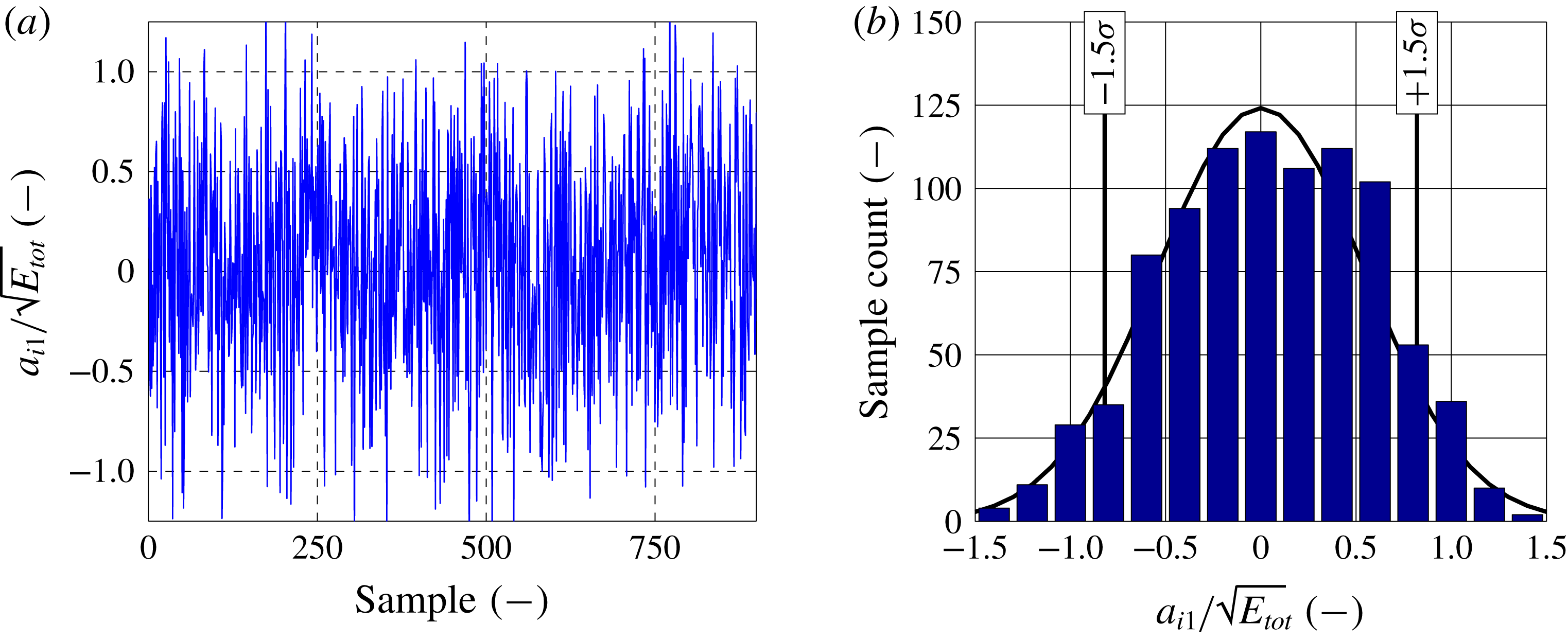
corner flow case in detail because it is often explored in other literature. In figure 16(a), we present the first POD mode coefficients (
 $a_{i1}/\sqrt{E_{tot}}$
) for the
 $24^{\circ }$
corner flow. We do not observe any clear trends in time for this or any POD mode. Additionally, we do not observe any clear phenomena when constructing phase portraits (two different POD mode coefficients plotted against one another), or transforming the POD mode coefficients into frequency space. One reason for not observing any interesting phenomena, such as the low-frequency dynamics discussed in Clemens & Narayanaswamy (Reference Clemens and Narayanaswamy2014), is a lack of temporal resolution. The laser repetition rate for this experiment is fixed to 10 Hz dictating a Nyquist frequency of 5 Hz, which is far slower than the characteristic time scales of this flow.
The sample distribution of energy for the first POD mode of the
 $24^{\circ }$
corner flow is presented in figure 16(b). There are no observable biases about the mean to within experimental error. Also in this figure, we mark the locations corresponding to 1.5 standard deviations (
 $1.5\unicode[STIX]{x1D70E}$
) of the
 $|a_{i1}|$
samples which have the largest magnitude; we will use the samples that correspond to these large coefficient values (positive and negative) to gain insight into the mean-flow behaviour exhibited by the POD modes.
First POD mode coefficients for
 $24^{\circ }$
corner flow. (a) Coefficients for POD mode
 $j=1$
,
 $a_{i1}$
versus sample number. (b) Sample distribution of coefficients for mode
 $j=1$
. Vertical black bars mark 1.5 standard deviations (
 $1.5\unicode[STIX]{x1D70E}$
) indicating large magnitude coefficients
 $|a_{i1}|$
.

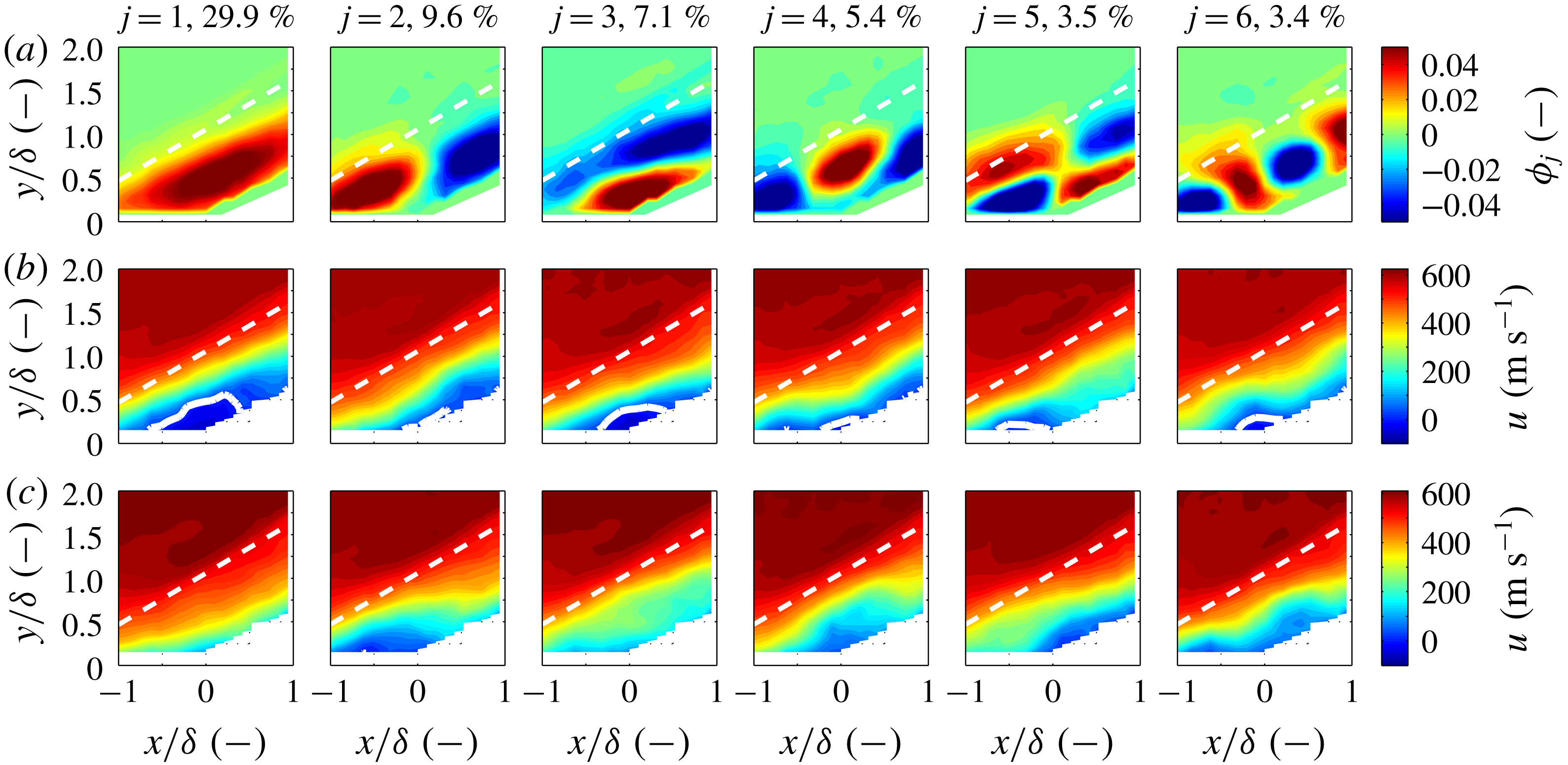
Snapshot POD analysis for the
 $24^{\circ }$
corner flow. Each column corresponds to one of the first six POD modes marked by the mode number
 $j$
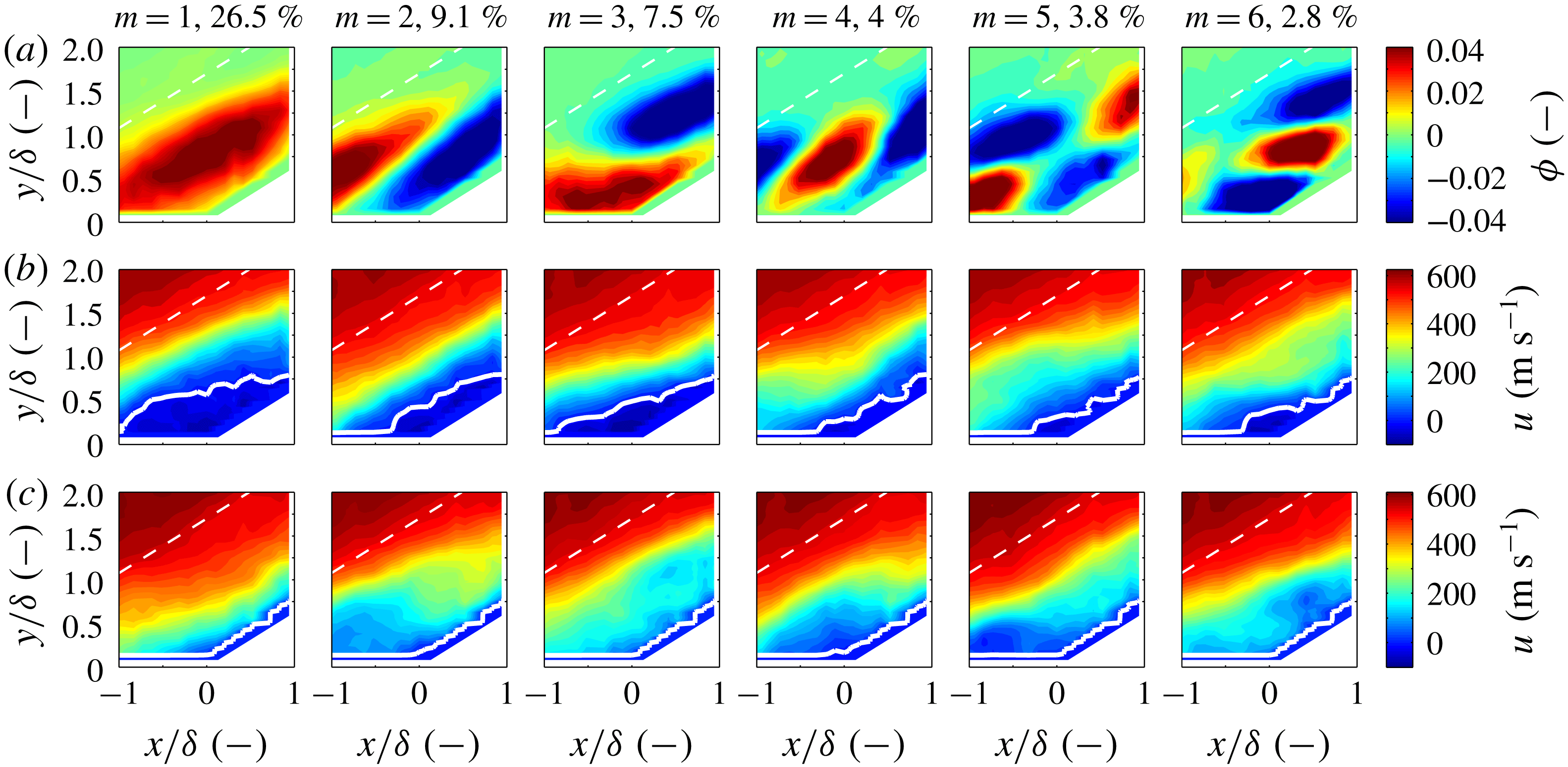
and the fraction of energy associated with each mode in %. (a) POD modes for the
 $24^{\circ }$
corner flow are shown as contours of
 $\unicode[STIX]{x1D719}_{j}$
. (b) The mean streamwise velocity of snapshots with the largest positive mode coefficients (samples falling to right of
 $+1.5\unicode[STIX]{x1D70E}$
in in figure 16). (c) The mean streamwise velocity of snapshots with the largest negative mode coefficients (samples falling to left of
 $-1.5\unicode[STIX]{x1D70E}$
in in figure 16). A solid white line denotes the boundary between positive and negative streamwise velocity. A dashed white line denotes the mean shock location.

The first six POD modes for the
 $24^{\circ }$
corner flow are shown as contours of
 $\unicode[STIX]{x1D719}_{j}$
in figure 17(a). To illustrate the effect of the different POD modes on the mean flow, the mean streamwise velocity of snapshots that correspond to the largest positive and negative mode coefficients is presented in figures 17(b) and 17(c) respectively. That is, in figure 17(b), we present the mean of the streamwise velocity of the snapshots corresponding to samples falling above 1.5 standard deviations of the POD mode coefficient distribution (
 $+1.5\unicode[STIX]{x1D70E}$
of
 $a_{i1}$
). And, in figure 17(c), we present the mean of the streamwise velocity of the snapshots corresponding to samples falling below 1.5 standard deviations of the POD mode coefficient distribution (
 $-1.5\unicode[STIX]{x1D70E}$
of
 $a_{i1}$
).
The first POD mode,
 $\unicode[STIX]{x1D719}_{1}$
, of the
 $24^{\circ }$
corner flow case appears in the first row of the first column in figure 17. Inspecting the mean-velocity field associated with large values of the mode coefficients, it appears that this POD mode is associated with large-scale filling (
 $+1.5\unicode[STIX]{x1D70E}$
of
 $a_{i1}$
, second row, first column of figure 17) and complete collapse (
 $-1.5\unicode[STIX]{x1D70E}$
of
 $a_{i1}$
, third row, first column of figure 17) of the separation bubble at the root of the corner. The second POD mode, (
 $\unicode[STIX]{x1D719}_{2}$
, second column of first row) appears to be the separation bubble oscillating in the streamwise direction as evidenced by the POD mode and the associated mean velocity fields associated with the large mode coefficients (
 $\pm 1.5\unicode[STIX]{x1D70E}$
of
 $a_{i2}$
). It appears that there is a sloshing, or shift in the streamwise direction of high and low momentum fluid. The third POD mode (
 $\unicode[STIX]{x1D719}_{3}$
, third column of first row) appears to be smaller-scale separation bubble filling and collapse in comparison with
 $\unicode[STIX]{x1D719}_{1}$
. There is an additional flow feature: when the flow is separated, there is a momentum surplus in the region immediately above the separation location and when the separation bubble is collapsed, there is a momentum deficit in the same region. This is potentially indicative of snapshots where the separation bubble is in the process of filling or collapsing. Modes
 $\unicode[STIX]{x1D719}_{4}$
and
 $\unicode[STIX]{x1D719}_{5}$
(fourth and fifth column of first row, respectively) appear to be harmonics of modes
 $\unicode[STIX]{x1D719}_{2}$
and
 $\unicode[STIX]{x1D719}_{3}$
, respectively. Mode
 $\unicode[STIX]{x1D719}_{6}$
(sixth column of first row, respectively) is difficult to interpret, but could be a harmonic of
 $\unicode[STIX]{x1D719}_{4}$
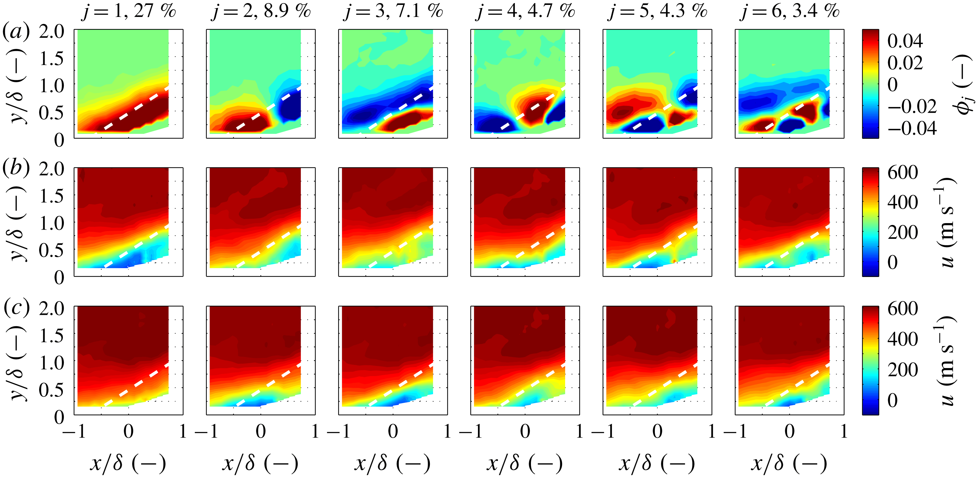
. Higher-order modes, not pictured here, indicate increasingly smaller structures within the boundary layer and shock layer. In some of the higher modes, there are thin structures which appear close to the mean shock location, but these structures are associated with POD modes containing less than 1 % of the TKE in the flow. That is, the energy associated with fluctuations from the mean shock location are small relative to the fluctuations associated with the dynamics of the separation bubble.
10 Comparison of POD analyses between cases
The POD analysis applied to the
 $24^{\circ }$
corner case that was presented in figure 17 is also applied to the
 $8^{\circ }$
corner,
 $16^{\circ }$
corner,
 $32^{\circ }$
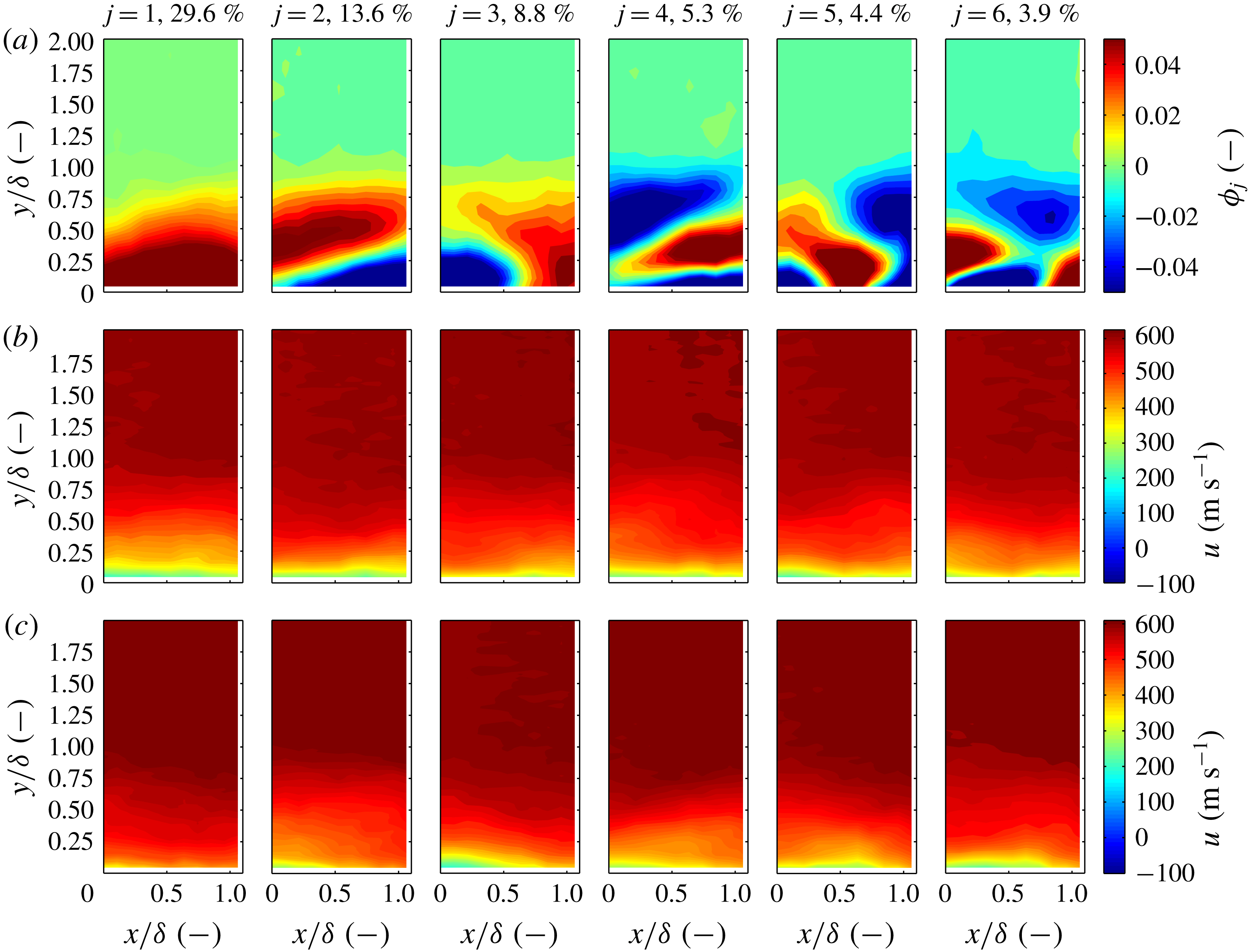
corner and boundary-layer cases and presented in figures 19–22, respectively.
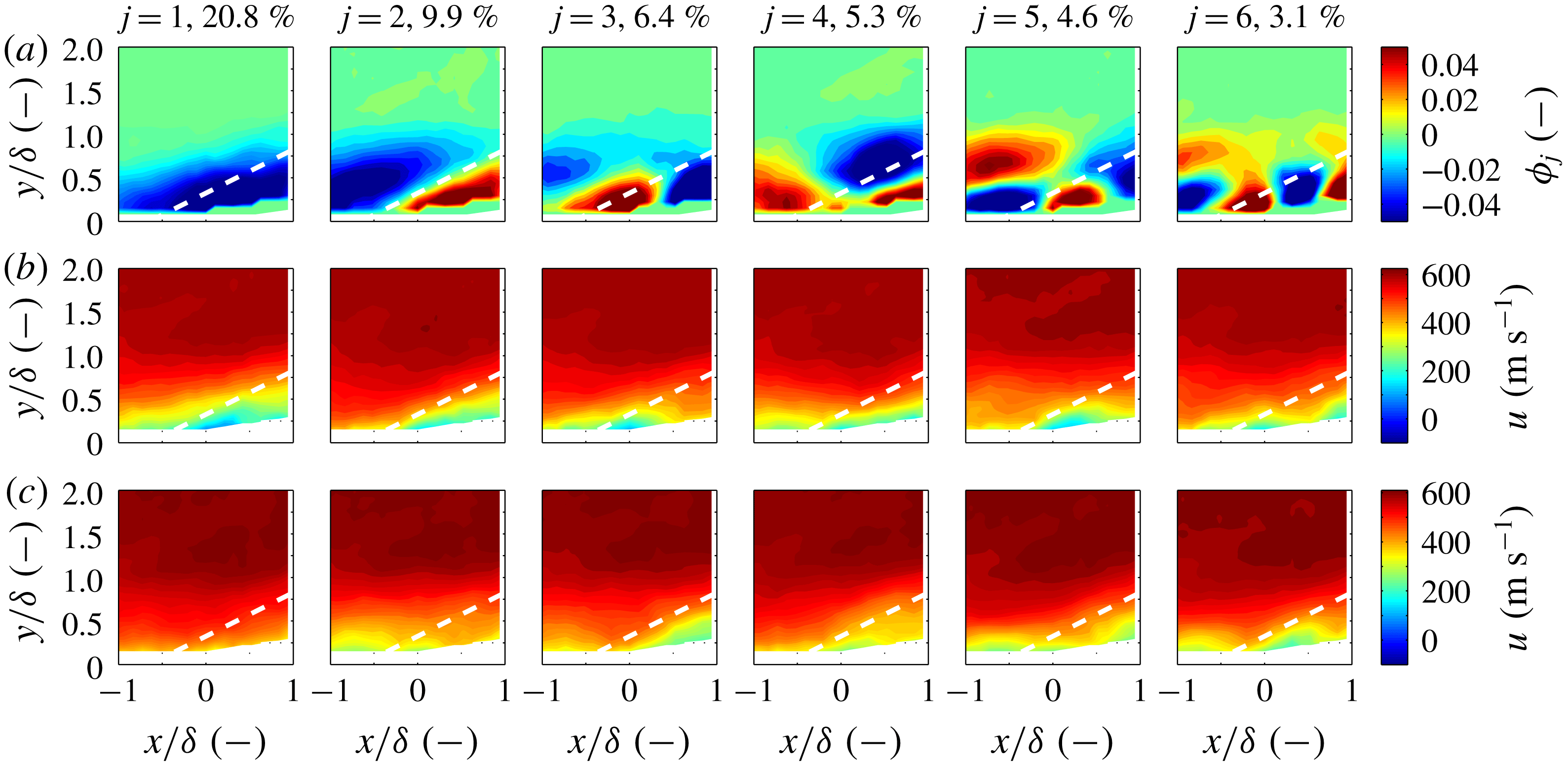
Several characteristics of the POD analyses are common among each of the cases. For all cases, the POD modes only register interesting content within the boundary layer and shock layer. This is a sensible result as the free-stream disturbances are small and incoherent relative to the disturbances within the shock and boundary layers. For mode number higher than approximately
 $j=10$
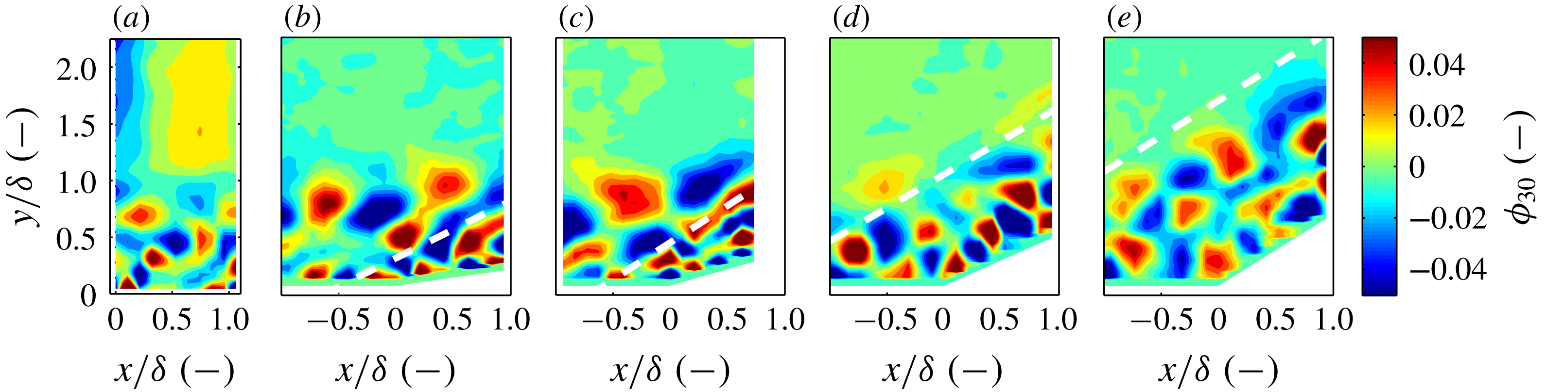
, the POD modes are difficult to distinguish from one case to another, besides the obvious change in boundary geometry. That is, the disturbances evident in the high-order POD modes appear quite similar between cases in terms of distribution, amplitude, and length scale. To illustrate this point, the 30th POD mode (
 $\unicode[STIX]{x1D719}_{30}$
) is presented in figure 18 for each of the cases. The qualitative observation of commonality of the higher POD modes is also evident in the spectra of the eigenvalues presented in figure 15(b). The initial thought was that the commonality of the higher-order modes was due to noise in the measurement technique, which is also common among all cases. However, the signal-to-noise ratio appears sufficient at high mode number (figure 18).
Comparison of the 30th POD mode (
 $\unicode[STIX]{x1D719}_{30}$
) among the boundary-layer and
 $8^{\circ }$
,
 $16^{\circ }$
,
 $24^{\circ }$
and
 $32^{\circ }$
corner flows, from left to right, respectively. A dashed white line denotes the mean shock location.

Several characteristics of the POD analyses are dissimilar between the cases. In contrast to the
 $16^{\circ }$
,
 $24^{\circ }$
and
 $32^{\circ }$
corner cases, the first POD of the
 $8^{\circ }$
corner does not appear to indicate a relatively large separation bubble. Additionally, in the
 $24^{\circ }$
and
 $32^{\circ }$
cases, the shock wave appears to extend the upper boundary of where turbulent structures appear in the flow (figure 18
d,e). This is juxtaposed to the
 $8^{\circ }$
and
 $16^{\circ }$
cases where this is not readily observed (figure 18
b,c).
Snapshot POD analysis for the
 $8^{\circ }$
corner flow. (a) POD modes are shown as contours of
 $\unicode[STIX]{x1D719}_{j}$
. (b,c) The mean streamwise velocity of snapshots that correspond to the largest positive and negative mode coefficients, respectively. A dashed white line denotes the mean shock location.

Snapshot POD analysis for the
 $16^{\circ }$
corner flow. (a) POD modes are shown as contours of
 $\unicode[STIX]{x1D719}_{j}$
. (b,c) The mean streamwise velocity of snapshots that correspond to the largest positive and negative mode coefficients, respectively. A dashed white line denotes the mean shock location.

Snapshot POD analysis for the
 $32^{\circ }$
corner flow. (a) POD modes are shown as contours of
 $\unicode[STIX]{x1D719}_{j}$
. (b,c) The mean streamwise velocity of snapshots that correspond to the largest positive and negative mode coefficients, respectively. A dashed white line denotes the mean shock location.

Snapshot POD analysis for the boundary-layer flow. Each column corresponds to one of the first six POD modes marked by the mode number
 $j$
and the fraction of energy associated with each mode in per cent. (a) POD modes are shown as contours of
 $\unicode[STIX]{x1D719}_{j}$
. (b,c) The mean streamwise velocity of snapshots that correspond to the largest positive and negative mode coefficients, respectively.

11 Conclusions
The incoming boundary layer and shock-wave/boundary-layer interactions over four compression corners at
 $M_{\infty }=2.8$
were investigated using one-dimensional KTV in the M3CT. The focus of this study was the effect of compression-corner angle on streamwise turbulent kinetic energy (sTKE) and structure in Mach 2.8 flow. This canonical flow may be observed in practice as the deflection of a control surface on a vehicle in high-speed flight or in the flow path of a high-speed, air-breathing engine.
Typical Z-type schlieren images were recorded for each compression-corner flow to address concerns about potential tunnel-starting issues in the M3CT. We found no such tunnel starting issues and made fits to the mean initial shock-wave angle. These data agreed with data in the literature, which built confidence in studying these geometries in the M3CT.
For the incoming boundary layer, data from ten mean- and fluctuating-velocity profiles spanning
 ${\approx}11~\text{mm}$
or
 $x/\unicode[STIX]{x1D6FF}\approx 1.1$
in the streamwise direction were reduced and compared to data from the literature. These comparisons included van Direst I scaling, Morkovin scaling of the streamwise-velocity fluctuations and longitudinal correlations. Comparisons are favourable between the KTV data collected in this work and experimental and computational data from the literature. From this, we concluded that the incoming flow could be nominally treated as a canonical supersonic, turbulent boundary layer and investigations of shock-wave/turbulent boundary-layer interactions could commence.
For the shock-wave/turbulent boundary-layer interactions, data from
 ${\approx}$
20 mean- and fluctuating-velocity profiles spanning
 ${\approx}22$
mm or
 $x/\unicode[STIX]{x1D6FF}\approx 2.1$
were recorded for compression-corner angles of
 $8^{\circ }$
,
 $16^{\circ }$
,
 $24^{\circ }$
and
 $32^{\circ }$
. This was an effective demonstration of extending the application of tagging velocimetry into a complex flow field.
For the
 $16^{\circ }$
,
 $24^{\circ }$
and
 $32^{\circ }$
cases, the shear layer near the root of interaction region was identified by fitting a coordinate system to the maxima of sTKE (
 $u_{rms}^{\prime 2}/(U_{2}^{2})$
). To a first approximation, we observed the shear-layer profiles were self-similar by using the streamwise fluctuations in the laboratory frame as a surrogate for streamwise fluctuations in the shear-layer frame, which was the approach in Helm et al. (Reference Helm, Martin and Dupont2014).
In an effort to identify trends of longitudinal turbulent stress with compression-corner angle, we defined a figure of merit termed the wall-normal integrated sTKE,
 $\overline{\text{sTKE}}$
. This figure of merit is intended to identify the overall longitudinal turbulent stress contained in the flow at different
 $x/\unicode[STIX]{x1D6FF}$
locations, which should be relatively easy to compare between other experimental and computational studies. Because
 $\overline{\text{sTKE}}$
is the wall-normal integrated value, it will capture the amplitude of
 $u_{rms}^{\prime 2}/(2U_{\infty }^{2})$
, in addition to the effect of the width of the shear layer in each case. We observe that the wall-normal integrated sTKE (
 $\overline{\text{sTKE}}$
) scales as an exponential with respect to the compression-corner angle.
Proper orthogonal decomposition (POD) of the streamwise-velocity data was used to examine the structures and spectra in the flow. Knight & Sirovich (Reference Knight and Sirovich1990) and Moser (Reference Moser1994) suggest that the POD eigenfunctions are a good set of basis functions with which to form an inertial-range spectrum for inhomogeneous, turbulent flows and such a spectrum was identified in this work. That is, we found the POD eigenspectra to scale as
 $\unicode[STIX]{x1D706}_{j}\propto j^{-11/9}$
which is analogous to the famous inertial-range scaling due to Kolmogorov (Kolmogorov Reference Kolmogorov1941) (
 $E\propto \unicode[STIX]{x1D716}^{2/3}k^{-5/3}$
). At a POD mode number greater than
 ${\approx}10$
there was an initially unanticipated similarity between the eigenspectra considering how dissimilar and inhomogeneous each case is (e.g. the boundary-layer flow versus the
 $32^{\circ }$
corner flow). However, upon close inspection, the first few POD modes do not clearly scale as
 $j^{-11/9}$
, and these modes contain the structures (inhomogeneity and separation) which strongly modify the mean flow. Following the first
 ${\approx}10$
modes, the similarity of the inertial range is apparent between each case.
To identify the modification of the mean flow due to each POD mode, we presented the mean streamwise velocity of the samples which correspond to the POD mode coefficients falling above and below 1.5 standard deviations (
 $\pm 1.5\unicode[STIX]{x1D70E}$
of
 $a_{ij}$
). We observed that the first several modes are somewhat similar between each compression-corner case (with the exception of the
 $8^{\circ }$
corner where the flow was mostly attached). These first POD modes contain most of the kinetic energy and are those that modify the mean flow, giving rise to features such as separation bubble filling/collapse and oscillation.
Acknowledgements
The M3CT facilities were supplied by the Arnold Engineering Development Complex (AEDC). The Air Force Summer Faculty Fellowship Program (SFFP) supported M.A.M. and N.J.P. with a stipend for this work. M.A.M. and N.J.P. were supported by AFOSR Young Investigator Program Grant FA9550-16-1-0262 and equipment for this work was supported by AFOSR DURIP Grant FA9550-15-1-0325; I. Leyva of AFOSR is the Program Manager for both grants. We acknowledge the machine work done by M. Simonovic and M. Reid of the Stevens Institute of Technology. We also would like to thank J. Brooks of the University of Maryland for assistance with operating the wind tunnel and the Pitot measurements. We would like to acknowledge the encouragement of J. Laffery and D. Marren of AEDC White Oak. Finally, we would like to acknowledge the reviewers for providing valuable insight into this work.
Supplementary movie
Supplementary movies are available at https://doi.org/10.1017/jfm.2018.1029.