3.2.1 Problem 1: first source term

When reducing equation (3.17) by taking into account the first source term only, the equation to be solved is

(3.19) $$\begin{eqnarray}\displaystyle \frac{\unicode[STIX]{x03C0}}{2}c_{0}\frac{\unicode[STIX]{x2202}^{3}\overline{u}_{1}}{\unicode[STIX]{x2202}{\hat{y}}^{3}}=\frac{\unicode[STIX]{x2202}^{2}(\overline{u^{\prime }u^{\prime }})}{\unicode[STIX]{x2202}\hat{x}\unicode[STIX]{x2202}{\hat{y}}}, & & \displaystyle\end{eqnarray}$$

with boundary conditions (3.11a,b )–(3.11d ), for $\overline{u}_{1}$ . Integrating equation (3.19) and using the boundary conditions yields the following simplified solution:

(3.20) $$\begin{eqnarray}\displaystyle \overline{u}_{1}(\hat{x},{\hat{y}}) & = & \displaystyle -\frac{U_{ac}^{2}}{16c_{0}}\sin (2\unicode[STIX]{x03C0}\hat{x})\left\{15\frac{{\hat{y}}^{2}}{\hat{R}^{3}}-\frac{15}{\hat{R}}-6\frac{{\hat{y}}^{2}}{\hat{R}^{2}}\right.\nonumber\\ \displaystyle & & \displaystyle +\left.2(1+2\text{e}^{2({\hat{y}}-\hat{R})}+8\text{e}^{{\hat{y}}-\hat{R}}\sin (\hat{R}-{\hat{y}}))\right\}.\end{eqnarray}$$

Along the axis, by normalizing with Rayleigh’s solution and neglecting smaller terms, we obtain at $O(1/\hat{R})$ :

(3.21) $$\begin{eqnarray}\displaystyle \frac{\overline{u}_{1}(\hat{x},0)}{\overline{u}_{R}}=\frac{2}{3}-\frac{5}{\hat{R}}. & & \displaystyle\end{eqnarray}$$

The second-order pressure gradient can also be obtained, and as expected is independent of ${\hat{y}}$ . It is given by

(3.22) $$\begin{eqnarray}\displaystyle \frac{\text{d}\overline{p}_{1}}{\text{d}\hat{x}}=\frac{\unicode[STIX]{x1D70C}_{0}\unicode[STIX]{x03C0}U_{ac}^{2}}{16}\sin (2\unicode[STIX]{x03C0}\hat{x})\left(8+\frac{6}{\hat{R}^{2}}-\frac{15}{\hat{R}^{3}}\right). & & \displaystyle\end{eqnarray}$$

3.2.2 Problem 2: second source term

The equation to be solved for the acoustic streaming issued from the second source term in equation (3.17) is

(3.23) $$\begin{eqnarray}\displaystyle \frac{\unicode[STIX]{x03C0}}{2}c_{0}\frac{\unicode[STIX]{x2202}^{3}\overline{u}_{2}}{\unicode[STIX]{x2202}{\hat{y}}^{3}}=\hat{L}\frac{\unicode[STIX]{x2202}^{2}(\overline{u^{\prime }v^{\prime }})}{\unicode[STIX]{x2202}{\hat{y}}^{2}}, & & \displaystyle\end{eqnarray}$$

with boundary conditions (3.11a,b )–(3.11d ) for $\overline{u}_{2}$ . Integrating (3.23) gives the following simplified expression for $\overline{u}_{2}$

(3.24) $$\begin{eqnarray}\displaystyle \overline{u}_{2}(\hat{x},{\hat{y}}) & = & \displaystyle -\frac{U_{ac}^{2}}{32c_{0}}\sin (2\unicode[STIX]{x03C0}\hat{x})\left\{\frac{1}{\hat{R}}+3\frac{{\hat{y}}^{2}}{\hat{R}^{3}}(1-2\hat{R})+2(1-2\text{e}^{2({\hat{y}}-\hat{R})})\right.\nonumber\\ \displaystyle & & \displaystyle +\left.\frac{4}{\hat{R}}\text{e}^{{\hat{y}}-\hat{R}}[(-1+2{\hat{y}})\cos (\hat{R}-{\hat{y}})+(1-2\hat{R})\sin (\hat{R}-{\hat{y}})]\right\}.\end{eqnarray}$$

Along the axis, we obtain at the order $O(1/\hat{R})$ :

(3.25) $$\begin{eqnarray}\displaystyle \frac{\overline{u}_{2}(\hat{x},0)}{\overline{u}_{R}}=\frac{1}{3}+\frac{1}{6\hat{R}}, & & \displaystyle\end{eqnarray}$$

and the corresponding pressure gradient is

(3.26) $$\begin{eqnarray}\displaystyle \frac{\text{d}\overline{p}_{2}}{\text{d}\hat{x}}=-\frac{\unicode[STIX]{x1D70C}_{0}\unicode[STIX]{x03C0}U_{ac}^{2}}{32}\sin (2\unicode[STIX]{x03C0}\hat{x})\left(\frac{4}{\hat{R}}-\frac{6}{\hat{R}^{2}}+\frac{3}{\hat{R}^{3}}\right). & & \displaystyle\end{eqnarray}$$

3.2.3 Analysis of the effect of the first two source terms

It is interesting to analyse the right-hand side of the axial component of the momentum equation in (3.10). For the first problem, the right-hand side is $\text{RHS}_{1}=\unicode[STIX]{x2202}\overline{p}_{1}/\unicode[STIX]{x2202}\hat{x}+\unicode[STIX]{x1D70C}_{0}(\unicode[STIX]{x2202}/\unicode[STIX]{x2202}\hat{x})(\overline{u^{\prime }u^{\prime }})$ . For the second problem, the right hand side is $\text{RHS}_{2}=\unicode[STIX]{x2202}\overline{p}_{2}/\unicode[STIX]{x2202}\hat{x}+\unicode[STIX]{x1D70C}_{0}\hat{L}(\unicode[STIX]{x2202}/\unicode[STIX]{x2202}{\hat{y}})(\overline{u^{\prime }v^{\prime }})$ .

The right-hand sides are therefore composed of two terms, a pressure gradient term and a Reynolds stress term. Figure 2 shows, for $\hat{R}=20$ , at $\hat{x}=-1/4$ , the transverse profile of both terms composing $\text{RHS}_{1}$ figures 2(a) and $\text{RHS}_{2}$ 2(b), normalized by $\unicode[STIX]{x1D70C}_{0}U_{ac}^{2}$ . Comparing figure 2(a,b) shows that the terms in $\text{RHS}_{2}$ are much smaller than in $\text{RHS}_{1}$ , and also that the pressure gradient and Reynolds stress terms almost compensate each other in the core of the guide, for both problems 1 and 2. The pressure gradients of problems 1 and 2 have opposite signs, and also $\text{d}\overline{p}_{2}/\text{d}\hat{x}$ is much smaller than $\text{d}\overline{p}_{1}/\text{d}\hat{x}$ , with $\text{d}\overline{p}_{2}/\text{d}\hat{x}\rightarrow 0$ when $\hat{R}$ becomes large (refer to equations (3.22) and (3.26)).

Figure 2(c) shows the transverse profile of the complete right-hand sides $\text{RHS}_{1}$ and $\text{RHS}_{2}$ , normalized by $\unicode[STIX]{x1D70C}_{0}U_{ac}^{2}$ , again for $\hat{R}=20$ , at $\hat{x}=-1/4$ . This figure shows that the two complete right-hand sides are of the same order, with significant values only near the wall. This stresses the fact that streaming is generated only by viscous boundary layer effects. The outer streaming is created from momentum diffusion of the velocity created near the guide wall, and not from pressure gradient effects. As stated by Menguy & Gilbert (Reference Menguy and Gilbert2000a ) (p. 253): pressure is created directly by the acoustic wave, and not by the mean flow. Outer streaming flow can thus be considered as a driven flow, similar to a Couette flow (see the driven cavity analogy developed in Daru et al. (Reference Daru, Weisman, Baltean-Carlès, Reyt and Bailliet2017b )).

The resulting normalized axial streaming velocity transverse profiles are plotted on figure 2(d). The following observation can be made: the first problem is responsible for the inner streaming (Schlichting streaming), while the second problem only contributes to the outer streaming (Rayleigh streaming), as also noticed in Paridaens et al. (Reference Paridaens, Kouidri and Jebali Jerbi2013). This is related to the fact that $\text{RHS}_{2}$ vanishes for ${\hat{y}}=\hat{R}$ , while $\text{RHS}_{1}$ does not, as can be seen in figure 2(c).

Figure 2.

Variation with ${\hat{y}}$ , for $\hat{x}=-1/4$ and $\hat{R}=20$ of (a) Reynolds stresses term (red solid line) and normalized pressure gradient term (red dashed line) in $\text{RHS}_{1}$ , (b) Reynolds stresses term (blue solid line) and normalized pressure gradient term (blue dashed line) in $\text{RHS}_{2}$ , (c) total normalized $\text{RHS}_{1}$ (red solid line) and $\text{RHS}_{2}$ (blue dashed line), (d) normalized axial streaming velocity $\overline{u}_{1}/\overline{u}_{R}$ (red solid line) and $\overline{u}_{2}/\overline{u}_{R}$ (blue dashed line).

Let us now consider the superposition of problems $1$ and $2$ considered above, which is usually assumed in the literature to give the total axial streaming velocity $\overline{u}_{1+2}=\overline{u}_{1}+\overline{u}_{2}$ . Figure 3 shows the normalized axial streaming velocity transverse profiles $\overline{u}_{1}$ , $\overline{u}_{2}$ and $\overline{u}_{1+2}$ . This figure also illustrates that the first problem is responsible for the inner streaming, while the second problem only contributes to the outer streaming: only $\overline{u}_{1}$ takes a positive value near the wall, while $\overline{u}_{2}$ remains negative.

The expression for $\overline{u}_{1+2}$ obtained on the axis is approximated as:

(3.27) $$\begin{eqnarray}\displaystyle \frac{\overline{u}_{1+2}(\hat{x},0)}{\overline{u}_{R}}=1-\frac{29}{6}\frac{1}{\hat{R}}. & & \displaystyle\end{eqnarray}$$

For large guides ( $\hat{R}\gg 1$ , but still $(\hat{R}/\hat{L})^{2}\ll 1$ ), we thus recover Rayleigh’s solution. As noticed by Lighthill (Reference Lighthill1978) and as shown by equations (3.21) and (3.25), the contributions of the first and second source terms in Rayleigh’s solution are respectively $2/3$ and $1/3$ . Equation (3.27) also shows a linear variation with $1/\hat{R}$ , which is not negligible for moderate values of $\hat{R}$ . The first source term is the main contributor to this dependency: $-5$ in (3.21) versus $1/6$ in (3.25).

Figure 3.

Axial streaming velocities $\overline{u}_{1}(-1/4,{\hat{y}})/\overline{u}_{R}$ (red solid line), $\overline{u}_{2}(-1/4,{\hat{y}})/\overline{u}_{R}$ (blue dashed line) and $\overline{u}_{1+2}(-1/4,{\hat{y}})/\overline{u}_{R}$ (black dot-dashed line). $\hat{R}=50$ .

The total axial pressure gradient is

(3.28) $$\begin{eqnarray}\displaystyle \frac{\text{d}\overline{p}_{1+2}}{\text{d}\hat{x}}=\frac{\unicode[STIX]{x1D70C}_{0}\unicode[STIX]{x03C0}U_{ac}^{2}}{2}\sin (2\unicode[STIX]{x03C0}\hat{x})\left(1-\frac{1}{8\hat{R}}+\frac{3}{16\hat{R}^{2}}-\frac{27}{32\hat{R}^{3}}\right). & & \displaystyle\end{eqnarray}$$

It follows that, for large values of $\hat{R}$

(3.29) $$\begin{eqnarray}\displaystyle \frac{\text{d}\overline{p}_{1+2}}{\text{d}\hat{x}}\simeq \frac{\text{d}\overline{p}_{1}}{\text{d}\hat{x}}=\frac{\unicode[STIX]{x1D70C}_{0}\unicode[STIX]{x03C0}U_{ac}^{2}}{2}\sin (2\unicode[STIX]{x03C0}\hat{x}). & & \displaystyle\end{eqnarray}$$

Integrating equation (3.29) with respect to $\hat{x}$ yields

(3.30) $$\begin{eqnarray}\displaystyle \overline{p}_{1+2}\simeq \overline{p}_{1}=p_{0}-\frac{\unicode[STIX]{x1D70C}_{0}U_{ac}^{2}}{4}\cos (2\unicode[STIX]{x03C0}\hat{x}). & & \displaystyle\end{eqnarray}$$

When scaling $\overline{p}_{1+2}-p_{0}$ by $(\unicode[STIX]{x1D6FE}/4)p_{0}(U_{ac}/c_{0})^{2}$ , we recover the theoretical result for the dimensionless hydrodynamic streaming pressure known in the literature $P_{2s}=-\text{cos}(2\unicode[STIX]{x03C0}\hat{x})$ (e.g. Menguy & Gilbert Reference Menguy and Gilbert2000a ).

3.2.4 Problem 3: third source term

We now consider the third source term, yielding the following equation

(3.31) $$\begin{eqnarray}\displaystyle \frac{\unicode[STIX]{x03C0}}{2}c_{0}\hat{L}\frac{\unicode[STIX]{x2202}^{3}\overline{u}_{3}}{\unicode[STIX]{x2202}{\hat{y}}^{3}}=-\frac{\unicode[STIX]{x2202}^{2}(\overline{u^{\prime }v^{\prime }})}{\unicode[STIX]{x2202}\hat{x}^{2}}, & & \displaystyle\end{eqnarray}$$

with boundary conditions (3.11a,b )–(3.11d ) for $\overline{u}_{3}$ . Integrating (3.31) gives the simplified solution

(3.32) $$\begin{eqnarray}\displaystyle \overline{u}_{3}(\hat{x},{\hat{y}}) & = & \displaystyle \frac{\unicode[STIX]{x03C0}^{2}U_{ac}^{2}}{480c_{0}}\frac{1}{\hat{L}^{2}}\sin (2\unicode[STIX]{x03C0}\hat{x})\left\{4\hat{R}^{3}+150-\frac{585}{\hat{R}}+\frac{720}{\hat{R}^{2}}\right.\nonumber\\ \displaystyle & & \displaystyle -\,3{\hat{y}}^{2}\left(\frac{240}{\hat{R}^{4}}-\frac{315}{\hat{R}^{3}}+\frac{150}{\hat{R}^{2}}+8\hat{R}\right)+60\text{e}^{2({\hat{y}}-\hat{R})}+20\frac{{\hat{y}}^{4}}{\hat{R}}\nonumber\\ \displaystyle & & \displaystyle +\left.20\text{e}^{{\hat{y}}-\hat{R}}\left(\left(12-\frac{18}{\hat{R}}\right)\cos (\hat{R}-{\hat{y}})-\frac{18}{\hat{R}}\sin (\hat{R}-{\hat{y}})+12\frac{{\hat{y}}}{\hat{R}}\sin (\hat{R}-{\hat{y}})\right)\right\}.\nonumber\\ \displaystyle & & \displaystyle\end{eqnarray}$$

Along the axis we obtain, neglecting terms of order $O(\text{e}^{-\hat{R}})$ and smaller

(3.33) $$\begin{eqnarray}\displaystyle \frac{\overline{u}_{3}(\hat{x},0)}{\overline{u}_{R}}=-\frac{2\unicode[STIX]{x03C0}^{2}}{45}\left(\frac{\hat{R}}{\hat{L}}\right)^{2}\left[\hat{R}+\frac{75}{2}-\frac{585}{4\hat{R}}+\frac{180}{\hat{R}^{2}}\right]. & & \displaystyle\end{eqnarray}$$

Since the term in brackets is always positive, velocity $\overline{u}_{3}$ is of the opposite sign to Rayleigh’s solution. Thus the associated vortices are reversed.

Note that in this equation the dominant term $\hat{R}(\hat{R}/\hat{L})^{2}$ could increase significantly for large values of $\hat{R}$ . However, our working hypotheses are that the linear regime of streaming is respected, that is $Re_{NL}=(M\hat{R})^{2}\ll 1$ , and also that $(\hat{R}/\hat{L})^{2}\ll 1$ . These relations imply that the product $\hat{R}(\hat{R}/\hat{L})^{2}$ and consequently the velocity component $\bar{u}_{3}$ will both remain bounded for large values of $\hat{R}$ .

The second-order pressure gradient in the $x$ direction can be calculated from

(3.34) $$\begin{eqnarray}\displaystyle \frac{\unicode[STIX]{x2202}\overline{p}_{3}}{\unicode[STIX]{x2202}\hat{x}}=\unicode[STIX]{x1D70C}_{0}\frac{\unicode[STIX]{x03C0}}{2}c_{0}\frac{\unicode[STIX]{x2202}^{2}\overline{u}_{3}}{\unicode[STIX]{x2202}{\hat{y}}^{2}}, & & \displaystyle\end{eqnarray}$$

yielding

(3.35) $$\begin{eqnarray}\displaystyle \frac{\unicode[STIX]{x2202}\overline{p}_{3}}{\unicode[STIX]{x2202}\hat{x}} & = & \displaystyle -\frac{\unicode[STIX]{x1D70C}_{0}\unicode[STIX]{x03C0}^{3}U_{ac}^{2}}{2\hat{L}^{2}}\sin (2\unicode[STIX]{x03C0}\hat{x})\left\{\frac{3}{\hat{R}^{4}}-\frac{63}{16\hat{R}^{3}}+\frac{15}{8\hat{R}^{2}}+\frac{\hat{R}}{10}-\frac{{\hat{y}}^{2}}{2\hat{R}}-\frac{1}{20}\text{e}^{2({\hat{y}}-\hat{R})}\right.\nonumber\\ \displaystyle & & \displaystyle +\left.\frac{1}{2}\text{e}^{{\hat{y}}-\hat{R}}\left(\frac{-1+2{\hat{y}}}{\hat{R}}\cos (\hat{R}-{\hat{y}})+\left(\frac{1}{\hat{R}}-2\right)\sin (\hat{R}-{\hat{y}})\right)\right\}.\end{eqnarray}$$

For this source term the axial pressure gradient (which is very small) does depend on  ${\hat{y}}$ .

3.2.5 Problem 4: fourth source term

Considering the fourth source term yields

(3.36) $$\begin{eqnarray}\displaystyle \frac{\unicode[STIX]{x03C0}}{2}c_{0}\hat{L}\frac{\unicode[STIX]{x2202}^{3}\overline{u_{4}}}{\unicode[STIX]{x2202}{\hat{y}}^{3}}=-\hat{L}\frac{\unicode[STIX]{x2202}^{2}(\overline{v^{\prime }v^{\prime }})}{\unicode[STIX]{x2202}\hat{x}\unicode[STIX]{x2202}{\hat{y}}}, & & \displaystyle\end{eqnarray}$$

with boundary conditions (3.11a,b )–(3.11d ) for $\overline{u}_{4}$ . Integrating equation (3.36) and using the boundary conditions, the following simplified solution is found:

(3.37) $$\begin{eqnarray}\displaystyle \overline{u}_{4}(\hat{x},{\hat{y}})=\frac{\unicode[STIX]{x03C0}^{2}U_{ac}^{2}}{120c_{0}}\sin (2\unicode[STIX]{x03C0}\hat{x})\left(\frac{\hat{R}}{\hat{L}}\right)^{2}\left[1-6\left(\frac{{\hat{y}}}{\hat{R}}\right)^{2}+5\left(\frac{{\hat{y}}}{\hat{R}}\right)^{4}\right]. & & \displaystyle\end{eqnarray}$$

Along the axis we obtain the following expression for the normalized axial streaming velocity

(3.38) $$\begin{eqnarray}\displaystyle \frac{\overline{u}_{4}(\hat{x},0)}{\overline{u}_{R}}=\frac{2\unicode[STIX]{x03C0}^{2}}{45}\left(\frac{\hat{R}}{\hat{L}}\right)^{2}. & & \displaystyle\end{eqnarray}$$

Comparing equations (3.38) and (3.33) shows that $\overline{u}_{4}(\hat{x},0)/\overline{u}_{R}$ is equal to $-1/\hat{R}$ times the first term of $\overline{u}_{3}(\hat{x},0)/\overline{u}_{R}$ . The contribution of the fourth source term is thus negligible for large enough guides.

3.2.6 Superposition of solutions

Gathering together the four components $\overline{u}_{1}$ , $\overline{u}_{2}$ , $\overline{u}_{3}$ and $\overline{u}_{4}$ , and neglecting the lower-order terms, the total streaming velocity along the axis is given by

(3.39) $$\begin{eqnarray}\displaystyle \frac{\overline{u}(\hat{x},0)}{\overline{u}_{R}}=\frac{\mathop{\sum }_{i=1}^{4}\overline{u}_{i}(\hat{x},0)}{\overline{u}_{R}}=1-\frac{29}{6}\frac{1}{\hat{R}}-\frac{2\unicode[STIX]{x03C0}^{2}}{45}\frac{\hat{R}^{3}}{\hat{L}^{2}}\left[1+\frac{73}{2\hat{R}}-\frac{585}{4\hat{R}^{2}}+\frac{180}{\hat{R}^{3}}\right]. & & \displaystyle\end{eqnarray}$$

This expression shows that, under certain circumstances, the streaming flow can be reversed on the axis ( $\overline{u}(\hat{x},0)/\overline{u}_{R}<0$ ). This occurs when

(3.40) $$\begin{eqnarray}\displaystyle \hat{L}<\hat{L}_{limit}=\unicode[STIX]{x03C0}\sqrt{\frac{2}{45}}\left(\frac{\hat{R}^{3}\left(1+\displaystyle \frac{73}{2\hat{R}}-\displaystyle \frac{585}{4\hat{R}^{2}}+\displaystyle \frac{180}{\hat{R}^{3}}\right)}{1-\displaystyle \frac{29}{6}\frac{1}{\hat{R}}}\right)^{1/2}. & & \displaystyle\end{eqnarray}$$

Figure 4 shows the variation with $\hat{R}$ of the limit value $\hat{L}_{limit}/\hat{R}$ . For geometries that fall under the curve, there exists a reversed flow on the axis. Minimum values are $\hat{R}=13.52,\hat{L}/\hat{R}=L/R=5.24$ . These values are compatible with the hypothesis $(\hat{R}/\hat{L})^{2}\ll 1$ . For example, for $\hat{R}=100$ , reversed outer streaming velocity occurs if $\hat{L}<789$ , or $L/R<7.89$ .

In order to characterize the possible applications, let us consider a practical case of reverse flow along the guide axis. Let $\hat{L}$ and $\hat{R}$ be fixed. For resonance conditions, $\unicode[STIX]{x1D706}=2L$ and $\unicode[STIX]{x1D714}=\unicode[STIX]{x03C0}c_{0}/L$ . Using $\unicode[STIX]{x1D6FF}_{\unicode[STIX]{x1D708}}^{2}=2\unicode[STIX]{x1D708}/\unicode[STIX]{x1D714}$ and $\hat{L}=L/\unicode[STIX]{x1D6FF}_{\unicode[STIX]{x1D708}}$ , the following equations are obtained

(3.41a,b ) $$\begin{eqnarray}\displaystyle L=\frac{2\unicode[STIX]{x1D708}}{\unicode[STIX]{x03C0}c_{0}}\hat{L}^{2},\quad R=L\frac{\hat{R}}{\hat{L}}. & & \displaystyle\end{eqnarray}$$

Let $\hat{L}=789$ and $\hat{R}=100$ , as previously. Taking standard values corresponding to air, $\unicode[STIX]{x1D708}=1.496\times 10^{-5}~\text{m}^{2}~\text{s}^{-1}$ and $c_{0}=343.82~\text{m}~\text{s}^{-1}$ , we obtain $L=17.2~\text{mm}$ , $R=2.15~\text{mm}$ and the resonance frequency $f=10~\text{kHz}$ . These dimensions are small and could concern microfluidics systems, where Rayleigh streaming is used, for example within the field of acoustic particle trapping and manipulation or efficient fluid mixing. It is interesting to remark that some experiments in microfluidics have shown Rayleigh streaming vortices rotating in the opposite direction to that expected. Our results could give an explanation to this phenomenon that is a subject of debate (Wiklund, Green & Ohlin Reference Wiklund, Green and Ohlin2012).

Figure 4.

Limit value $\hat{L}_{limit}(\hat{R})/\hat{R}$ under which the flow is reversed on the axis. Minimum values: $\hat{R}=13.52,\hat{L}_{limit}/\hat{R}=5.24$ .

Figure 5.

Axial streaming velocities $\overline{u}_{1}(\hat{x},{\hat{y}})/\overline{u}_{R}$ (red solid line), $\overline{u}_{2}(\hat{x},{\hat{y}})/\overline{u}_{R}$ (blue dashed line), $\overline{u}_{3}(\hat{x},{\hat{y}})/\overline{u}_{R}$ (green dotdashed line) and $\overline{u}_{4}(\hat{x},{\hat{y}})/\overline{u}_{R}$ (purple dotted line). $\hat{R}=50$ , $\hat{L}=500$ . (a) ${\hat{y}}=0$ ; (b) $\hat{x}=-1/4$ .

Figure 5 shows the four components $\overline{u}_{1}/\overline{u}_{R}$ , $\overline{u}_{2}/\overline{u}_{R}$ , $\overline{u}_{3}/\overline{u}_{R}$ and $\overline{u}_{4}/\overline{u}_{R}$ along the axis (a) and along ${\hat{y}}$ for $\hat{x}=-1/4$ (b). Here we have $\hat{R}=50$ and $\hat{L}=500$ . We notice that the fourth contribution is negligible, and that the third contribution is of the same order of magnitude as the second one. Figure 6 shows the total axial velocity $\overline{u}$ profile for $\hat{R}=100$ and two values of $\hat{L}$ : $\hat{L}=600$ and $\hat{L}=8000$ . The difference between the two profiles is important in the core of the guide, whereas in the very near wall region, both profiles are very close.

Figure 6.

Total normalized axial streaming velocity transverse profile $u(-1/4,{\hat{y}})/\overline{u}_{R}$ for $\hat{R}=100$ and $\hat{L}=600$ (solid line), $\hat{L}=8000$ (dashed line).

This feature was also observed (even though the acoustic regime and the geometric configuration were different) in experiments as well as numerical simulations, that revealed situations where the outer streaming flow was greatly modified (up to occurrence of reverse flow), while the inner streaming flow was nearly unmodified (Reyt et al. Reference Reyt, Daru, Bailliet, Moreau, Valière, Baltean-Carlès and Weisman2013; Reyt, Bailliet & Valière Reference Reyt, Bailliet and Valière2014).

At this stage we have shown that the usually neglected third source term of outer streaming is responsible for drastic change of behaviour of acoustic streaming for certain $(\hat{L},\hat{R})$ conditions. The ratio $R/\unicode[STIX]{x1D6FF}_{\unicode[STIX]{x1D708}}$ is usually considered as the criterion to differentiate between different streaming regimes, from narrow guides with only inner cells to large guides with mostly outer cells. The present study implies that not only $R/\unicode[STIX]{x1D6FF}_{\unicode[STIX]{x1D708}}$ but also $R/L$ ratios should be considered in order to examine the organization of the streaming flow.

In the following sections we consider the impact of this finding on other characteristics of streaming flow: slip velocity, mass transport velocity, vertical component of streaming velocity.

3.2.7 Slip velocity

The viscous boundary layer vortex thickness (inner streaming) was estimated to be approximatively equal to $1.9\unicode[STIX]{x1D6FF}_{\unicode[STIX]{x1D708}}$ by Schlichting (Reference Schlichting1932), who did not consider streaming outside the boundary layer. As shown by experiments (Moreau et al. Reference Moreau, Bailliet and Valière2008), the limit for large guides between inner and outer streaming cells is $3\unicode[STIX]{x1D6FF}_{\unicode[STIX]{x1D708}}$ from the wall, as illustrated in figure 1. At $3\unicode[STIX]{x1D6FF}_{\unicode[STIX]{x1D708}}$ from the guide wall, the axial streaming velocity was indeed found to reach its maximum. The flow in the core of the guide is initiated by transverse diffusion of momentum from there. This position is the limit between inner and outer streaming cells and the value of the axial streaming velocity at non-dimensional ${\hat{y}}={\hat{y}}^{l}=\hat{R}-3$ is thus generally considered as a slip velocity when inner streaming is not described. Rayleigh’s solution for the slip velocity is given by $\overline{u}_{R}^{SV}=(3/8)U_{ac}^{2}/c_{0}\sin (2\unicode[STIX]{x03C0}\hat{x})$ .

The actual non-dimensional transverse location ${\hat{y}}^{SV}$ of the maximum of the axial streaming velocity can however deviate from this standard value, depending on values of $\hat{R}$ and $\hat{L}$ . Figure 7 shows the difference (or offset) ${\hat{y}}^{SV}-{\hat{y}}^{l}$ between the actual and standard location of the slip velocity as a function of $\hat{R}$ (for $6<\hat{R}<200$ ), for two values of $\hat{L}$ . For the largest value of $\hat{L}$ , we note that the actual location shifts slightly away from the wall as $\hat{R}$ increases (it is placed at the standard value for $\hat{R}=28$ ). This is in agreement with previous results showing the evolution of the axial streaming velocity transverse profile with the ratio $R/\unicode[STIX]{x1D6FF}_{\unicode[STIX]{x1D708}}$ (e.g. figure 4 of Bailliet et al. (Reference Bailliet, Gusev, Raspet and Hiller2001) and figure 4 of Hamilton et al. (Reference Hamilton, Ilinskii and Zabolotskaya2003a )).

For the smallest value of $\hat{L}$ , the actual location of the slip velocity shifts closer to the wall as $\hat{R}$ increases. This can be related to the fact that the $\overline{u}_{3}$ contribution becomes large (see figure 5).

Figure 7.

Difference (or offset) between the actual location ${\hat{y}}^{SV}$ and the standard location $\hat{R}-3$ of the slip velocity, as a function of $\hat{R}$ . Solid line: $\hat{L}=8000$ , dashed line: $\hat{L}=500$ .

Figure 8 shows the axial slip velocity $\overline{u}$ , normalized by $\overline{u}_{R}^{SV}$ , at the actual position ${\hat{y}}={\hat{y}}^{SV}$ (corresponding to figure 7). It can be noted that the normalized value goes naturally to almost 1 as $\hat{R}$ becomes large for the largest value of $\hat{L}$ . However this is not the case for the smallest value of $\hat{L}$ and the normalized value is reduced significantly for $\hat{R}>50$ .

Figure 8.

Normalized axial slip velocity at position ${\hat{y}}={\hat{y}}^{SV}$ , as a function of $\hat{R}$ . Solid line: $\hat{L}=8000$ , dashed line: $\hat{L}=500$ .

Here again we explore the limit of validity of the classical approach by showing that both the position and the value of the slip velocity are dependent not only on $\hat{R}$ but also on $\hat{L}$ . This is stressed also by results shown in figure 9 that gives a comparison of the slip velocity and the maximum normalized axial velocity on the guide axis, for $\hat{L}=8000$ and $\hat{L}=500$ . We can see that the axial slip velocity departs from Rayleigh’s solution more than that on the axis for small values of $\hat{R}$ (the solid curve is below the dashed curve). For large values of $\hat{R}$ , the opposite is true: the slip velocity departs from Rayleigh’s solution less than the axial streaming velocity on the guide axis. Comparing figure 9 (a,b) shows that this tendency is emphasized for smaller values of $\hat{L}$ , due to increased importance of $\overline{u}_{3}$ .

Figure 9.

Normalized axial slip velocity versus $\hat{R}$ (solid line), and maximum normalized axial streaming velocity on the axis (dashed line). (a) $\hat{L}=8000$ , (b) $\hat{L}=500$ .

3.2.8 Average mass transport velocity

The streaming velocity considered up to now in this study, is often referred to as ‘Eulerian’ time-average velocity. The ‘average mass transport’ velocity, associated with streaming mass transport, is often considered, especially for thermoacoustic applications where heat transport due to streaming is the relevant quantity of interest. The axial component of the average mass transport velocity $\overline{u}^{M}$ , at the first order of approximation, is given by

(3.42) $$\begin{eqnarray}\displaystyle \overline{u}^{M}(\hat{x},{\hat{y}})=\overline{u}+\frac{\overline{\unicode[STIX]{x1D70C}^{\prime }u^{\prime }}}{\unicode[STIX]{x1D70C}_{0}}. & & \displaystyle\end{eqnarray}$$

Along the axis, using (3.12) and neglecting terms of order $O(\text{e}^{-\hat{R}})$ and lower, it follows that

(3.43) $$\begin{eqnarray}\displaystyle \frac{\overline{u}^{M}(\hat{x},0)}{\overline{u}_{R}}=1-\frac{11}{2}\frac{1}{\hat{R}}-\frac{2\unicode[STIX]{x03C0}^{2}}{45}\frac{\hat{R}^{2}}{\hat{L}^{2}}\left[\hat{R}-1+\frac{30}{\hat{R}^{2}}-\frac{60}{\hat{R}^{3}}+\frac{45}{\hat{R}^{4}}\right]. & & \displaystyle\end{eqnarray}$$

Figure 10.

Axial velocities $\overline{u}^{M}(-1/4,{\hat{y}})/\overline{u}_{R}$ (dashed line), $\overline{u}(-1/4,{\hat{y}})/\overline{u}_{R}$ (solid line). (a)  $\hat{R}=6$ , $\hat{L}=8000$ , (b)  $\hat{R}=50$ , $\hat{L}=8000$ , (c)  $\hat{R}=90$ , $\hat{L}=8000$ , (d)  $\hat{R}=6$ , $\hat{L}=500$ , (e)  $\hat{R}=50$ , $\hat{L}=500$ , (f)  $\hat{R}=90$ , $\hat{L}=500$ .

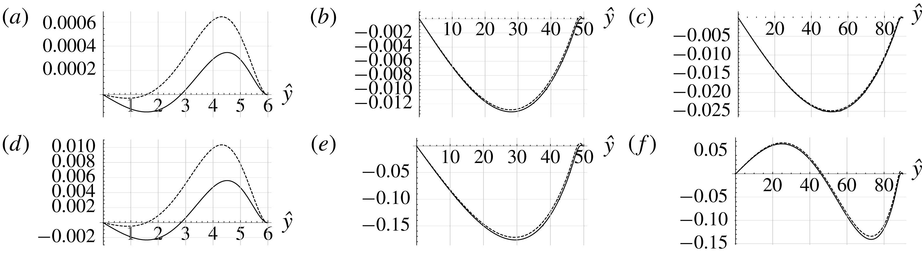
Figure 10 shows the transverse profiles of axial streaming velocities $\overline{u}$ and $\overline{u}^{M}$ , for three values of $\hat{R}$ (6, 50 and 90), and two values of $\hat{L}$ (8000 and 500). The difference between $\overline{u}$ and $\overline{u}^{M}$ is most significant in the viscous boundary layer, as usually considered. For small values of $\hat{R}$ , differences are significant everywhere, including on the axis. These differences between $\overline{u}$ and $\overline{u}^{M}$ are obviously associated with the additional term $\overline{\unicode[STIX]{x1D70C}^{\prime }u^{\prime }}$ . As shown by expressions (3.4) and (3.6) this term is nearly zero since it is the product of two terms nearly in quadrature apart from viscous boundary layers effects. Indeed on the axis the acoustic velocity oscillates as $\cos (2\unicode[STIX]{x03C0}\hat{t})$ (see dominant terms in equation (3.4)) and the acoustic density oscillates as $\sin (2\unicode[STIX]{x03C0}\hat{t})$ (see dominant terms in equation (3.6)). This feature is associated with the standing wave character of the oscillation in the guide under study that is closed at both ends and excited at its resonance frequency. In such resonators acoustic pressure (and thus density oscillations) are in quadrature with acoustic velocity due to boundary layers effects. Therefore for large guides (see figure 10 b,c,e,f) the difference between $\overline{u}$ and $\overline{u}^{M}$ is only significant close to the wall. For narrow guides, the inner streaming takes up most of the guide, thus $\overline{u}$ and $\overline{u}^{M}$ are different through the whole guide section (see figure 10 a,d).

Also in the case $\hat{R}=90$ and $\hat{L}=500$ (figure 10 f), the change of sign of $\overline{u}$ at ${\hat{y}}\approx 25$ indicates the appearance of a new vortex with reverse flow near the axis.

3.2.9 Vertical streaming velocity

It can also be useful to consider the vertical component of streaming velocity, especially to detect the appearance of new cells. Let us define the average mass transport vertical velocity variable given by, in the first order of approximation

(3.44) $$\begin{eqnarray}\displaystyle \overline{v}^{M}(\hat{x},{\hat{y}})=\overline{v}+\frac{\overline{\unicode[STIX]{x1D70C}^{\prime }v^{\prime }}}{\unicode[STIX]{x1D70C}_{0}}. & & \displaystyle\end{eqnarray}$$

The continuity equation (first equation in (3.10)) becomes

(3.45) $$\begin{eqnarray}\displaystyle \frac{\unicode[STIX]{x2202}\overline{u}^{M}}{\unicode[STIX]{x2202}\hat{x}}+\hat{L}\frac{\unicode[STIX]{x2202}\overline{v}^{M}}{\unicode[STIX]{x2202}{\hat{y}}}=0. & & \displaystyle\end{eqnarray}$$

Integrating equation (3.45) and using the boundary conditions (3.11c ) yields the simplified expression

(3.46) $$\begin{eqnarray}\displaystyle \overline{v}^{M}(\hat{x},{\hat{y}}) & = & \displaystyle \frac{\unicode[STIX]{x03C0}U_{ac}^{2}}{16c_{0}\hat{L}}\cos (2\unicode[STIX]{x03C0}\hat{x})\left\{\frac{{\hat{y}}}{\hat{R}}\left(-33+6\hat{R}-4\unicode[STIX]{x03C0}^{2}\frac{\hat{R}^{4}}{\hat{L}^{2}}\right)+\frac{{\hat{y}}^{3}}{\hat{R}^{3}}\left(11-6\hat{R}+\frac{8\unicode[STIX]{x03C0}^{2}}{15}\frac{\hat{R}^{4}}{\hat{L}^{2}}\right)\right.\nonumber\\ \displaystyle & & \displaystyle -\,\frac{4\unicode[STIX]{x03C0}^{2}}{15}\frac{\hat{R}^{4}}{\hat{L}^{2}}\frac{{\hat{y}}^{5}}{\hat{R}^{5}}+\text{e}^{{\hat{y}}-\hat{R}}\left[\cos (\hat{R}-{\hat{y}})\left(16+4\frac{{\hat{y}}}{\hat{R}}\right)+\sin (\hat{R}-{\hat{y}})\left(16-4\frac{{\hat{y}}}{\hat{R}}\right)\right]\nonumber\\ \displaystyle & & \displaystyle +\left.2\text{e}^{2({\hat{y}}-\hat{R})}\right\}.\end{eqnarray}$$

The Eulerian velocity $\overline{v}$ can be obtained using (3.44) and (3.13). Figure 11 shows the vertical velocities $\overline{v}$ and $\overline{v}^{M}$ for several values of $\hat{R}$ and two values of $\hat{L}$ . For small values of $\hat{R}$ (figure 11 a,d), $\overline{v}$ and $\overline{v}^{M}$ are very different. Also in the case $\hat{R}=90$ and $\hat{L}=500$ (figure 11 f), the change of sign of $\overline{v}$ and $\overline{v}^{M}$ at ${\hat{y}}\approx 46$ indicates the appearance of a new vortex with reverse flow near the axis.

Figure 11.

Vertical average mass transport velocities $\overline{v}^{M}(-1/2,{\hat{y}})/\overline{u}_{R}$ (dashed line), $\overline{v}(-1/2,{\hat{y}})/\overline{u}_{R}$ (solid line). (a)  $\hat{R}=6$ , $\hat{L}=8000$ , (b)  $\hat{R}=50$ , $\hat{L}=8000$ , (c)  $\hat{R}=90$ , $\hat{L}=8000$ , (d)  $\hat{R}=6$ , $\hat{L}=500$ , (e)  $\hat{R}=50$ , $\hat{L}=500$ , (f)  $\hat{R}=90$ , $\hat{L}=500$ .

Finally, as a summary, figure 12 shows the streamlines of the streaming flow plotted using (3.42) and (3.46), for $\hat{R}=90$ and $\hat{L}=500$ and $8000$ . For such large values of $\hat{R}$ , the inner streaming is restrained in a very small region near the wall. For $\hat{L}=8000$ , Rayleigh streaming is composed of two counter-rotating vortices as usual, while for $\hat{L}=500$ it is composed of four vortices, the flow along the axis being reversed.

Figure 12.

Streamlines of the mass transport velocity for $\hat{R}=90$ ; $\hat{L}=500$ (a), $\hat{L}=8000$  (b). (c) Zoom on the inner region of top figure.