3.1. Point source

The first perturbation is a point mass source located at ${\boldsymbol{x}_0}$. In unbounded space, the response to this perturbation is given by the free-space solution:

(3.6)\begin{equation}\delta U_{free}^{(1)}{\kern 1pt} = \left( {\begin{array}{*{20}{@{}c@{}}} {\delta p_{free}^{(1)}{\kern 1pt} }\\ \begin{array}{l} \rho \delta u_{free}^{(1)}\\ \rho \delta v_{free}^{(1)} \end{array} \end{array}} \right) = \frac{\varepsilon }{{2{\rm \pi} }}\left( {\begin{array}{*{20}{@{}c@{}}} { - (u{\partial_x} + v{\partial_y})(\ln r){\kern 1pt} }\\ \begin{array}{l} {\partial_x}\ln r\\ {\partial_y}\ln r \end{array} \end{array}} \right),\end{equation}

($r = |\boldsymbol{x} - {\boldsymbol{x}_0}|$ and $\varepsilon$ is an arbitrary constant point singularity strength that we introduce for convenience and that we will set to 1 in the end), which obeys the following linearized equations:

(3.7)\begin{equation}\begin{array}{@{}ccccc@{}} \boldsymbol{\nabla }\boldsymbol{\cdot }(\boldsymbol{A}\delta U_{free}^{(1)}) & = \left( {\begin{array}{*{20}{@{}c@{}}} {\rho \boldsymbol{\nabla }\boldsymbol{\cdot }\delta \boldsymbol{v}_{free}^{(1)}}\\ {\rho \boldsymbol{v}\boldsymbol{\cdot }\boldsymbol{\nabla }\delta {\kern 1pt} u_{free}^{(1)} + \rho u\boldsymbol{\nabla }\boldsymbol{\cdot }\delta \boldsymbol{v}_{free}^{(1)} + \rho \delta \boldsymbol{v}_{free}^{(1)}\boldsymbol{\cdot }\boldsymbol{\nabla }{\kern 1pt} u + {\partial_x}\delta p_{free}^{(1)}}\\ {\rho \boldsymbol{v}\boldsymbol{\cdot }\boldsymbol{\nabla }\delta {\kern 1pt} v_{free}^{(1)} + \rho v\boldsymbol{\nabla }\boldsymbol{\cdot }\delta \boldsymbol{v}_{free}^{(1)} + \rho \delta \boldsymbol{v}_{free}^{(1)}\boldsymbol{\cdot }\boldsymbol{\nabla }v + {\partial_y}\delta p_{free}^{(1)}} \end{array}} \right)\\ & = \varepsilon \left( {\begin{array}{*{20}{c}} 1\\ u\\ v \end{array}} \right)\delta (\boldsymbol{x} - {\boldsymbol{x}_0}) + \frac{\varepsilon }{{2{\rm \pi} }}\left( {\begin{array}{*{20}{@{}c@{}}} 0\\ {({\partial_y}u - {\partial_x}v){\partial_y}\ln r}\\ { - ({\partial_y}u - {\partial_x}v){\partial_x}\ln r} \end{array}} \right), \end{array}\end{equation}

where the second term on the right-hand side vanishes if the base flow is irrotational. Hence, the source vector is

(3.8)\begin{equation}{f^{(1)}} = \varepsilon \left( {\begin{array}{*{20}{c}} 1\\ u\\ v \end{array}} \right).\end{equation}

Notice that ${\psi ^T}{f^{(1)}} = \varepsilon ({\psi _1} + \boldsymbol{v}\boldsymbol{\cdot }\boldsymbol{\varphi })$, so ${I^{(1)}}$ is related to the (continuous) adjoint-based lift/drag gradient (2.12).

The Green's function approach requires the value of the linearized functionals ${I^{(1)}}$, which are the lift and drag forces exerted by the point source on a body. In the presence of a body, the above functional form (3.6) only holds locally near the singularity, such that (3.8) still holds, but needs to be modified globally to account for the wall boundary condition. This is particularly simple in 2-D potential flow using a complex variable and the method of images, and allows us to compute the force on immersed bodies using Blasius theorem (Milne-Thomson Reference Milne-Thomson1962). The simplest problem where the body is a circle is a standard academic exercise, and more general situations can be derived from this with suitable conformal transformations. The complex force on the cylinder turns out to be ${w_I} - {q_\infty }\,{\textrm{e}^{ - \textrm{i}\alpha }}$, where w_I is the induced velocity at the point singularity and ${q_\infty }\,{\textrm{e}^{ - \textrm{i}\alpha }}$ is the free stream complex velocity (here ${q_\infty } = \sqrt {u_\infty ^2 + v_\infty ^2}$). An interesting fact is that the same expression yields the force on a body of arbitrary shape (Milne-Thomson Reference Milne-Thomson1962), a result that is known as Lagally's theorem. Hence, the force exerted by the point source on the body is, keeping only terms linear in the source strength $\varepsilon$,

(3.9)\begin{equation}\delta {D^{(1)}} - i\delta {L^{(1)}} = \varepsilon \,{\textrm{e}^{\textrm{i}\alpha }}(u - iv - {q_\infty }\,{\textrm{e}^{ - \textrm{i}\alpha }}) + O({\varepsilon ^2}).\end{equation}

Here, δD ⁽¹⁾ and δL ⁽¹⁾ stand for the linear perturbations to drag and lift, respectively, due to the point source. Equation (3.9) thus gives the linearized force exerted by a point source on a rigid body of arbitrary shape in terms of the undisturbed velocity at the source, $u - iv$. This is not the end of the story though. Potential flows contain circulation, which can be freely adjusted a priori. For bodies with sharp trailing edges, the value of the circulation is fixed by the Kutta condition that asserts that the flow contains the precise amount of circulation to make the flow smooth at the trailing edge. The introduction of a point source disturbs the flow at the trailing edge, so the circulation has to be adjusted accordingly to preserve the smooth flow at the trailing edge. The extra circulation contributes an additional term to (3.9) that we shall calculate shortly. For blunt bodies, however, the circulation is not fixed by any smoothness requirement. However, it turns out that to obtain consistent adjoint solutions, a Kutta condition has to be imposed as well, ensuring no perturbation to the position of the rear stagnation point (see § 3.2.1).

To obtain explicit formulae, we will consider an airfoil in the complex z plane with a sharp trailing edge at z = 1. Let us suppose that the airfoil is transformed into a circle of radius R and centred at ${\zeta _0}$ in the auxiliary complex $\zeta $-plane by a conformal mapping $z = F(\zeta )$ (with $F(\zeta ) \to 1\;\textrm{as}\;|\zeta |\to \infty $), such that the point ${\zeta _{te}}$ on the circle is transformed into the trailing edge of the airfoil at z = 1. The (irrotational) base flow around the circle can be derived from the complex potential:

(3.10)\begin{equation}\varPhi (\zeta ) = {q_\infty }\,{\textrm{e}^{ - \textrm{i}\alpha }}(\zeta - {\zeta _0}) + {q_\infty }\,{\textrm{e}^{\textrm{i}\alpha }}\frac{{{R^2}}}{{\zeta - {\zeta _0}}} - \frac{{i{\varGamma _0}}}{{2{\rm \pi} }}\ln (\zeta - {\zeta _0}).\end{equation}

The corresponding potential at a point z on the airfoil plane is precisely $\varPhi (\zeta (z))$. In the unperturbed flow, the circulation ${\varGamma _0}$ around the circle has to be fixed to the value

(3.11)\begin{equation}{\varGamma _0} ={-} 2{\rm \pi} i{q_\infty }\,{\textrm{e}^{ - \textrm{i}\alpha }}({\zeta _{te}} - {\zeta _0}) + 2{\rm \pi} i{q_\infty }\,{\textrm{e}^{\textrm{i}\alpha }}\frac{{{R^2}}}{{{\zeta _{te}} - {\zeta _0}}},\end{equation}

such that the flow around the circle has a stagnation point at ${\zeta _{te}}$, i.e.

(3.12)\begin{equation}W({\zeta _{te}}) = \textrm{d}\varPhi /\textrm{d}\zeta {|_{\zeta = {\zeta _{te}}}} = {q_\infty }\,{\textrm{e}^{ - \textrm{i}\alpha }} - {q_\infty }\,{\textrm{e}^{\textrm{i}\alpha }}\frac{{{R^2}}}{{{{({\zeta _{te}} - {\zeta _0})}^2}}} - \frac{{i{\varGamma _0}}}{{2{\rm \pi} }}\frac{1}{{{\zeta _{te}} - {\zeta _0}}} = 0.\end{equation}

After inserting a point source at ${\zeta _s}$, the potential picks an extra contribution from the point source and its images with respect to the circle (Milne-Thomson Reference Milne-Thomson1962):

(3.13)\begin{equation}{\varPhi _s}(\zeta ) = \frac{\varepsilon }{{2{\rm \pi} \rho }}\ln (\zeta - {\zeta _s}) + \frac{\varepsilon }{{2{\rm \pi} \rho }}\ln \left( {\zeta - {\zeta_0} - \frac{{{R^2}}}{{\overline {{\zeta_s}} - \overline {{\zeta_0}} }}} \right) - \frac{\varepsilon }{{2{\rm \pi} \rho }}\ln (\zeta - {\zeta _0}),\end{equation}

where $\bar{\zeta }$ denotes the complex conjugate of $\zeta $. Here, ${\varPhi _s}(\zeta )$ induces a non-zero velocity at ${\zeta _{te}}$,

(3.14)\begin{equation}{W_s}({\zeta _{te}}) = \frac{\varepsilon }{{2{\rm \pi} \rho ({\zeta _{te}} - {\zeta _s})}} + \frac{\varepsilon }{{2{\rm \pi} \rho }}\frac{1}{{{\zeta _{te}} - {\zeta _0} - \frac{{{R^2}}}{{\overline {{\zeta _s}} - \overline {{\zeta _0}} }}}} - \frac{\varepsilon }{{2{\rm \pi} \rho ({\zeta _{te}} - {\zeta _0})}},\end{equation}

which has to be cancelled with additional circulation

(3.15)\begin{equation}\delta {\varGamma _0} ={-} 2{\rm \pi} i({\zeta _{te}} - {\zeta _0}){W_s}({\zeta _{te}}).\end{equation}

This extra circulation produces an extra force that has to be added to (3.9):

(3.16)\begin{align}& \delta {D^{(1)}} - i\delta {L^{(1)}} = i\rho {q_\infty }\delta {\varGamma _0} + \varepsilon \,{\textrm{e}^{\textrm{i}\alpha }}(u - iv - {q_\infty }\,{\textrm{e}^{ - \textrm{i}\alpha }}) + O({\varepsilon ^2})\nonumber\\ & \quad = 2{\rm \pi} \rho {q_\infty }({\zeta _{te}} - {\zeta _0}){W_s}({\zeta _{te}}) + \varepsilon \,{\textrm{e}^{\textrm{i}\alpha }}(u - iv - {q_\infty }\,{\textrm{e}^{ - \textrm{i}\alpha }}) + O({\varepsilon ^2})\nonumber\\ & \quad ={-} \varepsilon {q_\infty }\left( {\dfrac{{{\zeta_{te}} - {\zeta_0}}}{{{\zeta_s} - {\zeta_{te}}}} - \dfrac{{\overline {{\zeta_{te}}} - \overline {{\zeta_0}} }}{{\overline {{\zeta_s}} - \overline {{\zeta_{te}}} }}} \right) + \varepsilon \,{\textrm{e}^{\textrm{i}\alpha }}(u - iv - {q_\infty }\,{\textrm{e}^{ - \textrm{i}\alpha }}) + O({\varepsilon ^2}). \end{align}

Notice that the extra term is purely imaginary, so it only affects lift. Separating the real and imaginary parts, setting $\varepsilon = 1$ and dividing by ${c_\infty }$ to normalize, we get the following linearized functionals due to the point source:

(3.17)\begin{equation}\left. {\begin{array}{*{20}{c@{}}} {I_D^{(1)}(z(\zeta )) = {\textstyle{1 \over {{c_\infty }}}}(u(z(\zeta ))\cos \alpha + v(z(\zeta ))\sin \alpha - {q_\infty }),}\\ {I_L^{(1)}(z(\zeta )) = {\textstyle{1 \over {{c_\infty }}}}(v(z(\zeta ))\cos \alpha - u(z(\zeta ))\sin \alpha ) - i{\textstyle{{{q_\infty }} \over {{c_\infty }}}}\left( {\dfrac{{{\zeta_{te}} - {\zeta_0}}}{{\zeta (z) - {\zeta_{te}}}} - \dfrac{{\overline {{\zeta_{te}}} - \overline {{\zeta_0}} }}{{\overline \zeta (z) - \overline {{\zeta_{te}}} }}} \right).} \end{array}} \right\}\end{equation}

Notice that the extra contribution is independent of the initial circulation and blows up at the trailing edge, thus providing a precise mechanism (and an explanation) for the adjoint singularity at the trailing edge.

3.2. Point vortex

The second perturbation is a point vortex. In unbounded space it is simply

(3.18)\begin{equation}\delta U_{free}^{(2)}{\kern 1pt} = \left( {\begin{array}{*{20}{@{}c@{}}} {\delta p_{free}^{(2)}{\kern 1pt} }\\ \begin{array}{l} \rho \delta u_{free}^{(2)}\\ \rho \delta v_{free}^{(2)} \end{array} \end{array}} \right) = \frac{\varepsilon }{{2{\rm \pi} }}\left( {\begin{array}{*{20}{@{}c@{}}} {(v{\partial_x} - u{\partial_y})(\ln r)}\\ \begin{array}{l} {\partial_y}\ln r\\ - {\partial_x}\ln r \end{array} \end{array}} \right).\end{equation}

This solution obeys the linearized equation

(3.19)\begin{equation}\begin{array}{@{}ccccc@{}} \boldsymbol{\nabla }\boldsymbol{\cdot }(\boldsymbol{A}\delta U_{free}^{(2)}) & = \left( {\begin{array}{*{20}{c}} {\rho \boldsymbol{\nabla }\boldsymbol{\cdot }\delta \boldsymbol{v}_{free}^{(2)}}\\ {\rho \boldsymbol{v}\boldsymbol{\cdot }\boldsymbol{\nabla }\delta {\kern 1pt} u_{free}^{(2)} + \rho u\boldsymbol{\nabla }\boldsymbol{\cdot }\delta \boldsymbol{v}_{free}^{(2)} + \rho \delta \boldsymbol{v}_{free}^{(2)}\boldsymbol{\cdot }\boldsymbol{\nabla }u + {\partial_x}\delta p_{free}^{(2)}}\\ {\rho \boldsymbol{v}\boldsymbol{\cdot }\boldsymbol{\nabla }\delta {\kern 1pt} v_{free}^{(2)} + \rho v\boldsymbol{\nabla }\boldsymbol{\cdot }\delta \boldsymbol{v}_{free}^{(2)} + \rho \delta \boldsymbol{v}_{free}^{(2)}\boldsymbol{\cdot }\boldsymbol{\nabla }v + {\partial_y}\delta p_{free}^{(2)}} \end{array}} \right)\\ & = \varepsilon \left( {\begin{array}{*{20}{@{}c@{}}} 0\\ v\\ { - u} \end{array}} \right)\delta (\boldsymbol{x} - {\boldsymbol{x}_0}) + \frac{\varepsilon }{{2{\rm \pi} }}\left( {\begin{array}{*{20}{@{}c@{}}} 0\\ {({\partial_x}v - {\partial_y}u){\partial_x}\ln r}\\ {({\partial_x}v - {\partial_y}u){\partial_y}\ln r} \end{array}} \right), \end{array}\end{equation}

where the extra term vanishes if the base flow is irrotational. Hence, the source vector is

(3.20)\begin{equation}{f^{(2)}} = \varepsilon \left( {\begin{array}{*{20}{@{}c@{}}} 0\\ v\\ { - u} \end{array}} \right).\end{equation}

Notice that ${\psi ^T}{f^{(2)}} = \varepsilon (v{\psi _2} - u{\psi _3})$, so ${I^{(2)}}$ approaches $q\hat{\textit{n}}_{S}\boldsymbol{\cdot }\boldsymbol{\varphi }$ as the vortex approaches the wall. Its value is thus constrained by the adjoint wall boundary condition ${\hat{n}_S}\boldsymbol{\cdot }\boldsymbol{\varphi } = c_\infty ^{ - 1}(\boldsymbol{d}\boldsymbol{\cdot }{\hat{n}_S})$ (Giles & Pierce Reference Giles and Pierce1997).

Once again, in the presence of a body, the above functional form needs to be modified to account for the wall boundary condition. The correct expression can then be used to compute the force exerted by the vortex on a body, which poses no significant difficulties relative to the source case, so we just quote the results. The linearized complex force, taking into account the Kutta condition, is

(3.21)\begin{align}\delta {D^{(2)}} - i\delta {L^{(2)}} & = 2{\rm \pi} \rho {q_\infty }({\zeta _{te}} - {\zeta _0}){W_\nu }({\zeta _{te}}) + i\varepsilon \,{\textrm{e}^{\textrm{i}\alpha }}(u - iv - {q_\infty }\,{\textrm{e}^{ - \textrm{i}\alpha }}) + O({\varepsilon ^2})\nonumber\\ & ={-} i\varepsilon {q_\infty }\left( {\dfrac{{{\zeta_{te}} - {\zeta_0}}}{{{\zeta_s} - {\zeta_{te}}}} + \dfrac{{\overline {{\zeta_{te}}} - \overline {{\zeta_0}} }}{{\overline {{\zeta_s}} - \overline {{\zeta_{te}}} }}} \right) + i\varepsilon \,{\textrm{e}^{\textrm{i}\alpha }}(u - iv - {q_\infty }\,{\textrm{e}^{ - \textrm{i}\alpha }}) + O({\varepsilon ^2}), \end{align}

where ${W_\nu }({\zeta _{te}})$ is the complex velocity induced by the vortex (and its images) at ${\zeta _{te}}$. Hence, the properly normalized linearized functionals due to the vortex are (setting $\varepsilon = 1$)

(3.22)\begin{equation}\left. {\begin{array}{*{20}{c@{}}} {I_D^{(2)}(\zeta ) = {\textstyle{1 \over {{c_\infty }}}}(v(z(\zeta ))\cos \alpha - u(z(\zeta ))\sin \alpha )}\\ {I_L^{(2)}(z(\zeta )) ={-} {\textstyle{1 \over {{c_\infty }}}}(u(z(\zeta ))\cos \alpha + v(z(\zeta ))\sin \alpha - {q_\infty }) + {\textstyle{{{q_\infty }} \over {{c_\infty }}}}\left( {\dfrac{{{\zeta_{te}} \!-\! {\zeta_0}}}{{{\zeta_s} \!-\! {\zeta_{te}}}} + \dfrac{{\overline {{\zeta_{te}}} \!-\! \overline {{\zeta_0}} }}{{\overline {{\zeta_s}} \!-\! \overline {{\zeta_{te}}} }}} \right)} \end{array}} \right\}\!.\end{equation}

Notice that the extra term diverges as the vortex approaches the trailing edge. Notice that along the wall, we have $|{\zeta _s} - {\zeta _0}|= R$ and, thus,

(3.23)\begin{equation}\frac{{{\zeta _{te}} - {\zeta _0}}}{{{\zeta _s} - {\zeta _{te}}}} + \frac{{\overline {{\zeta _{te}}} - \overline {{\zeta _0}} }}{{\overline {{\zeta _s}} - \overline {{\zeta _{te}}} }} ={-} 1,\end{equation}

so that

(3.24)\begin{equation}I_L^{(2)}{|_{wall}} ={-} {\textstyle{1 \over {{c_\infty }}}}(u\cos \alpha + v\sin \alpha ),\end{equation}

as required by the adjoint wall boundary condition.

3.3. Change in stagnation pressure at fixed p

For the final perturbation we choose, in analogy with Giles & Pierce (Reference Giles and Pierce1997), a perturbation to the stagnation pressure ${p_0} = p + {\textstyle{1 \over 2}}\rho {q^2}$ (where ${q^2} = {u^2} + {v^2}$) at fixed values of the pressure and the local flow angle $\phi $. As stagnation pressure is convected along streamlines, we expect the solution to be concentrated along the streamline downstream of the insertion point ${\boldsymbol{x}_0}$. Following Giles & Pierce (Reference Giles and Pierce1997), we use curvilinear streamline coordinates in which s is the distance along the streamline downstream of the insertion point and n is the coordinate perpendicular to the streamline. In these coordinates, the perturbation is, in a first approximation,

(3.25)\begin{equation}\varepsilon H(s)\delta (n)\frac{1}{q}{\left( {\frac{{\partial U}}{{\partial {p_0}}}} \right)_{p,\phi }}(\boldsymbol{x}) = \frac{\varepsilon }{{{q^3}}}\left( {\begin{array}{*{20}{c}} 0\\ u\\ v \end{array}} \right)(\boldsymbol{x})H(s)\delta (n),\end{equation}

where $H(s)$ is the Heaviside step function and $\delta (n)$ is the Dirac delta function. However, as explained in Giles & Pierce (Reference Giles and Pierce1997), this is not the full form of the solution. This fact can be understood most simply by noting that (3.25) does not obey the linearized flow equations. In fact,

(3.26)\begin{equation}\boldsymbol{\nabla }\boldsymbol{\cdot }\left[ {\frac{\varepsilon }{q}\boldsymbol{A}{{\left( {\frac{{\partial U}}{{\partial {p_0}}}} \right)}_{p,\phi }}H(s)\delta (n)} \right] = \boldsymbol{\nabla }\boldsymbol{\cdot }[\hat{s}{f^{(3)}}H(s)\delta (n)],\end{equation}

where $\hat{s}$ is the unit vector in the flow direction and

(3.27)\begin{equation}{f^{(3)}} = \frac{\varepsilon }{q}{\left( {\frac{{\partial \boldsymbol{F}\boldsymbol{\cdot }\hat{s}}}{{\partial {p_0}}}} \right)_{p,\phi }} = \frac{\varepsilon }{{{q^2}}}\left( {\begin{array}{*{20}{c}} 1\\ {2u}\\ {2v} \end{array}} \right).\end{equation}

To proceed further, we need to express $\boldsymbol{\nabla }$ in streamline coordinates. While for smooth functions $\boldsymbol{\nabla }\boldsymbol{\cdot }[\hat{s}w] = {\partial _s}w + w{\partial _n}\phi$, when delta functions are present, one needs to proceed more carefully. To this end, we follow Emanuel (Reference Emanuel2000) and define coordinates ξ ₁ along the streamline and ξ ₂ that parameterizes the lines orthogonal to ξ ₁. The ξ_i coordinates are related to the streamline coordinates as $\textrm{d}s = {h_1}\,\textrm{d}{\xi _1}$ and $\textrm{d}n = {h_2}\,\textrm{d}{\xi _2}$, where ${h_i} = ||\partial \boldsymbol{x}/\partial {\xi _i}||$ are the scale factors. In terms of $({\xi _1},{\xi _2})$, the divergence operator acting on a vector $\boldsymbol{w}$ is

(3.28)\begin{equation}\boldsymbol{\nabla }\boldsymbol{\cdot }\boldsymbol{w} = \frac{1}{{{h_1}{h_2}}}\frac{\partial }{{\partial {\xi _1}}}({h_2}\boldsymbol{w}\boldsymbol{\cdot }{\hat{e}_1}) + \frac{1}{{{h_1}{h_2}}}\frac{\partial }{{\partial {\xi _2}}}({h_1}\boldsymbol{w}\boldsymbol{\cdot }{\hat{e}_2}),\end{equation}

where ${\hat{e}_i} = h_i^{ - 1}\partial \boldsymbol{x}/\partial {\xi _i}$ are the local curvilinear unit basis vectors (note that ${\hat{e}_1} \equiv \hat{s}$ in earlier notation). Finally, we need to consider the Heaviside and Dirac delta functions. Since $\int\!\!\!\int {\textrm{d}\kern0.7pt x\,\textrm{d}y} = \int\!\!\!\int {{h_1}{h_2}\,\textrm{d}{\xi _1}\,\textrm{d}{\xi _2}} $, we have

(3.29)\begin{equation}\delta (\boldsymbol{x}) \equiv \delta (x)\delta (y) = \delta ({\xi _1})\delta ({\xi _2})/{h_1}{h_2},\end{equation}

and

(3.30)\begin{equation}H(s)\delta (n) \equiv H({\xi _1})\delta ({\xi _2})/{h_2}.\end{equation}

Hence,

(3.31)\begin{align}& \boldsymbol{\nabla }\boldsymbol{\cdot }({f^{(3)}}\hat{s}H(s)\delta (n)) = \dfrac{1}{{{h_1}{h_2}}}\dfrac{\partial }{{\partial {\xi _1}}}(H({\xi _1})\delta ({\xi _2}){f^{(3)}})\nonumber\\ & \quad = \dfrac{1}{{{h_1}{h_2}}}\delta ({\xi _1})\delta ({\xi _2}){f^{(3)}} + \dfrac{{H({\xi _1})\delta ({\xi _2})}}{{{h_2}}}\dfrac{1}{{{h_1}}}\dfrac{\partial }{{\partial {\xi _1}}}{f^{(3)}}\nonumber\\ & \quad = \delta (\boldsymbol{x} - {\boldsymbol{x}_0}){f^{(3)}} + H(s)\delta (n)\dfrac{\partial }{{\partial s}}{f^{(3)}}. \end{align}

Using $(u,v) = (q\cos \phi ,q\sin \phi )$, the last term on the right-hand side can be further expanded as

(3.32)\begin{equation}\frac{\partial }{{\partial s}}{f^{(3)}} = {f^{(1)}}{\partial _s}{q^{ - 2}} - \frac{2}{{{q^2}}}{f^{(2)}}{\partial _s}\phi ,\end{equation}

where

(3.33a,b)\begin{equation}{f^{(1)}} = \varepsilon \left( {\begin{array}{*{20}{c}} 1\\ u\\ v \end{array}} \right),\quad {f^{(2)}} = \varepsilon \left( {\begin{array}{*{20}{c}} 0\\ v\\ { - u} \end{array}} \right),\end{equation}

are the source vectors for the point source and vortex, respectively. Hence, we can write the full solution as

(3.34)\begin{align}& \delta {U^{(3)}}(\boldsymbol{x},{\boldsymbol{x}_0}) = \varepsilon H(s)\delta (n)\dfrac{1}{q}{\left( {\dfrac{{\partial U}}{{\partial {p_0}}}} \right)_{p,\phi }}(\boldsymbol{x})\nonumber\\ & \quad \quad - \iint {{h_1}{h_2}\,\textrm{d}{{\xi ^{\prime}}_1}\,\textrm{d}{{\xi ^{\prime}}_2}\dfrac{{H({{\xi ^{\prime}}_1} - \xi _1^0)\delta ({{\xi ^{\prime}}_2} - \xi _2^0)}}{{{h_2}}}{\partial _s}{q^{ - 2}}(\boldsymbol{x^{\prime}})\delta {U^{(1)}}(\boldsymbol{x},\boldsymbol{x^{\prime}})} \nonumber\\ & \quad \quad + \iint {{h_1}{h_2}\,\textrm{d}{{\xi ^{\prime}}_1}\,\textrm{d}{{\xi ^{\prime}}_2}\dfrac{{H({{\xi ^{\prime}}_1} - \xi _1^0)\delta ({{\xi ^{\prime}}_2} - \xi _2^0)}}{{{h_2}}}\dfrac{2}{{{q^2}}}{\partial _s}\phi (\boldsymbol{x^{\prime}})\delta {U^{(2)}}(\boldsymbol{x},\boldsymbol{x^{\prime}})} \nonumber\\ & \quad = \varepsilon H(s)\delta (n)\dfrac{1}{q}{\left( {\dfrac{{\partial U}}{{\partial {p_0}}}} \right)_{p,\phi }}(\boldsymbol{x}) - \int_0^\infty {\textrm{d}s^{\prime}{\partial _s}{q^{ - 2}}(\boldsymbol{x}(s^{\prime}))\delta {U^{(1)}}(\boldsymbol{x},\boldsymbol{x}(s^{\prime}))} \nonumber\\ & \quad \quad + \int_0^\infty {\textrm{d}s^{\prime}\dfrac{2}{{{q^2}}}{\partial _s}\phi (\boldsymbol{x}(s^{\prime}))\delta {U^{(2)}}(\boldsymbol{x},\boldsymbol{x}(s^{\prime}))} , \end{align}

where $\delta {U^{(1)}}$, $\delta {U^{(2)}}$ are the complete point source and point vortex Green's functions (i.e. respecting the wall boundary conditions), which reduce to (3.6) and (3.18), respectively, in the vicinity of the singularity. We can check that (3.34) obeys

(3.35)\begin{equation}\boldsymbol{\nabla }\boldsymbol{\cdot }(\boldsymbol{A}\delta {U^{(3)}}(\boldsymbol{x},{\boldsymbol{x}_0})) = {f^{(3)}}(\boldsymbol{x})\delta (\boldsymbol{x} - {\boldsymbol{x}_0}) = {f^{(3)}}({\boldsymbol{x}_0})\delta (\boldsymbol{x} - {\boldsymbol{x}_0}),\end{equation}

as expected. Notice that ${(\partial \rho q/\partial {p_0})_{p,\phi }} = 1/q$ so that ${\partial _s}{q^{ - 2}} = {\partial _s}[(1/q){(\partial \rho q/\partial {p_0})_{p,\phi }}] = \rho {\kern 1pt} {\partial _s}\tilde{m}$, where $\tilde{m}$ is the linearized mass flux perturbation defined in Giles & Pierce (Reference Giles and Pierce1997), and thus the first integral on the right-hand side of (3.34) is actually the integral derived in Giles & Pierce (Reference Giles and Pierce1997). The second integral also has an analogue in the compressible case, so the solution shown in Giles & Pierce (Reference Giles and Pierce1997) is apparently incomplete.

For pressure-based functionals, the first term in (3.34) does not contribute to the linearized functional, which can then be written as

(3.36)\begin{equation}{I^{(3)}}({\boldsymbol{x}_0}) ={-} \int_0^\infty {\textrm{d}s{\partial _s}{q^{ - 2}}(\boldsymbol{x}(s)){I^{(1)}}(\boldsymbol{x}(s))} + \int_0^\infty {\textrm{d}s\frac{2}{{{q^2}}}{\partial _s}\phi (\boldsymbol{x}(s)){I^{(2)}}(\boldsymbol{x}(s))} .\end{equation}

Again, the first integral on the right-hand side of (3.36) is equivalent to the corresponding integral in Giles & Pierce (Reference Giles and Pierce1997), where it was used to argue that there is a potential divergence along the incoming stagnation streamline. Whether this singularity is actually present or not depends on the cost function and the flow conditions. Numerical tests show that lift-adjoint solutions seem to have these singularities even in incompressible and irrotational flow, while drag-adjoint solutions only show them in certain transonic cases (Lozano & Ponsin Reference Lozano and Ponsin2021b).

We can now substitute (3.17) and (3.22) into (3.36) to compute the linearized functional corresponding to the stagnation pressure point perturbation (3.34). For drag, we get

(3.37)\begin{equation}I_D^{(3)} ={-} \frac{1}{{{q^2}{q_\infty }{c_\infty }}}{(\boldsymbol{v} - {\boldsymbol{v}_\infty })^2},\end{equation}

while for lift, the result is

(3.38)\begin{equation}I_L^{(3)}({\boldsymbol{x}_0}) ={-} \frac{2}{{{q^2}{c_\infty }}}(u\sin \alpha - v\cos \alpha ) + {\textstyle{{{q_\infty }} \over {{c_\infty }}}}\varXi ,\end{equation}

where

(3.39)\begin{equation}\varXi ={-} \int_0^\infty {\textrm{d}s{\partial _s}{q^{ - 2}}(\boldsymbol{x}(s)){\varUpsilon ^{(1)}}(\boldsymbol{x}(s))} + 2\int_0^\infty {\textrm{d}s\frac{1}{{{q^2}}}{\partial _s}\phi (\boldsymbol{x}(s))(1 + {\varUpsilon ^{(2)}}(\boldsymbol{x}(s)))} ,\end{equation}

and

(3.40) \begin{equation}\left. {\begin{array}{*{20}{c@{}}} {\varUpsilon^{(1)}}(z) ={-} i\left( {\dfrac{{{\zeta_{te}} - {\zeta_0}}}{{\zeta (z) - {\zeta_{te}}}} - \dfrac{{\overline {{\zeta_{te}}} - \overline {{\zeta_0}} }}{{\overline \zeta (z) - \overline {{\zeta_{te}}} }}} \right)\\ = 2\dfrac{{{X_{te}}({Y_0} - Y) + {X_0}(Y - {Y_{te}}) + X({Y_{te}} - {Y_0})}}{{{{(X - {X_{te}})}^2} + {{(Y - {Y_{te}})}^2}}},\\ {\varUpsilon^{(2)}}(z) = \dfrac{{{\zeta_{te}} - {\zeta_0}}}{{\zeta (z) - {\zeta_{te}}}} + \dfrac{{\overline {{\zeta_{te}}} - \overline {{\zeta_0}} }}{{\overline \zeta (z) - \overline {{\zeta_{te}}} }}\\ = 2\dfrac{{(X - {X_0})(X - {X_{te}}) + (Y - {Y_0})(Y - {Y_{te}}) - {{(X - {X_{te}})}^2} - {{(Y - {Y_{te}})}^2}}}{{{{(X - {X_{te}})}^2} + {{(Y - {Y_{te}})}^2}}}. \end{array}} \right\}\end{equation}

In (3.39), the integration is carried out along the streamline downstream of ${\boldsymbol{x}_0}$. Finally, X and Y in (3.40) are the Cartesian coordinates on the circle plane, in terms of which $\zeta = X + iY$.

4.1. Behaviour of Ξ

The streamline integral equation (3.39) represents the contribution to lift, due to the Kutta condition, of a unit point perturbation to the stagnation pressure. This perturbation generates secondary point sources and vortices along the streamline downstream of the insertion point. The contributions of these secondary perturbations to the lift (see (3.17), (3.22)) diverge near the trailing edge, which gives rise to a singular behaviour of Ξ near the dividing streamline upstream of the trailing edge or rear stagnation point (which includes the wall and the incoming stagnation streamline). Along the stagnation streamline upstream of the body, the integral is not defined, as the streamline splits up in two at the stagnation point, while along the wall, the integral diverges. For a circle, for example, the integral along the wall is

(4.10)\begin{equation}\varXi ({\boldsymbol{x}_0}) \sim \int_0^{{\theta _0}} {\textrm{d}\theta {{\cos }^2}(\theta /2)\cot \theta {{\csc }^3}\theta } ,\end{equation}

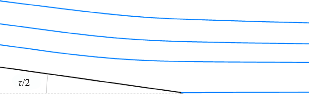
where ${\boldsymbol{x}_0} = (R\cos {\theta _0},R\sin {\theta _0})$, which diverges as ${\theta ^{ - 3}}$ at the rear stagnation point $(\theta = 0)$. Away from the dividing streamline, the integral grows unbounded as the corresponding streamline approaches the dividing streamline. To investigate the character of the divergence, we consider a simplified setup involving flow past a wedge of half-angle $\tau /2$ (figure 1).

Figure 1.

Streamlines for potential flow past a wedge of angle τ.

The asymptotic form of the complex potential for this case is ${z^{2/k}}$, where $k = 2 - \tau /{\rm \pi} $, so that stream function reads, in polar coordinates, $\psi = {r^{2/k}}\sin (2\theta /k)$, from which it follows that the minimum distance from a particular streamline to the trailing edge is ${r_{min}} \sim {\psi ^{k/2}}$, while the distance from a given point on the streamline to the dividing streamline is $d \sim \psi \sim r_{min}^{2/k}$. Likewise, the flow speed behaves as $q = O({r^{2/k - 1}})$, so ${\partial _s}q = O({r^{2/k - 2}}),$ and likewise ${\partial _s}\phi = O({r^{ - 1}})$. Finally, $\zeta \sim {z^{1/k}}$ and, thus, ${\varUpsilon ^{(1)}} = O({r^{ - 1/k}})$ and ${\varUpsilon ^{(2)}} = O({r^{ - 1/k}})$, so integrating along a streamline,

(4.11)\begin{equation}\varXi \sim r_{min}^{2 - 5/k} \sim r_{min}^{ - (2\tau /{\rm \pi} + 1)/(2 - \tau /{\rm \pi} )},\end{equation}

which depends on the trailing edge wedge angle $\tau $. Notice that the exponent is always negative for $0 < \tau \le {\rm \pi}$. It is thus clear that $\varXi $ has a potential divergence as the streamline approaches the dividing streamline. Let us consider three different scenarios in terms of the relative position of ${\boldsymbol{x}_0}$.

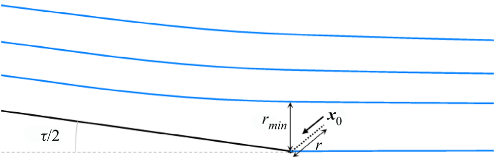
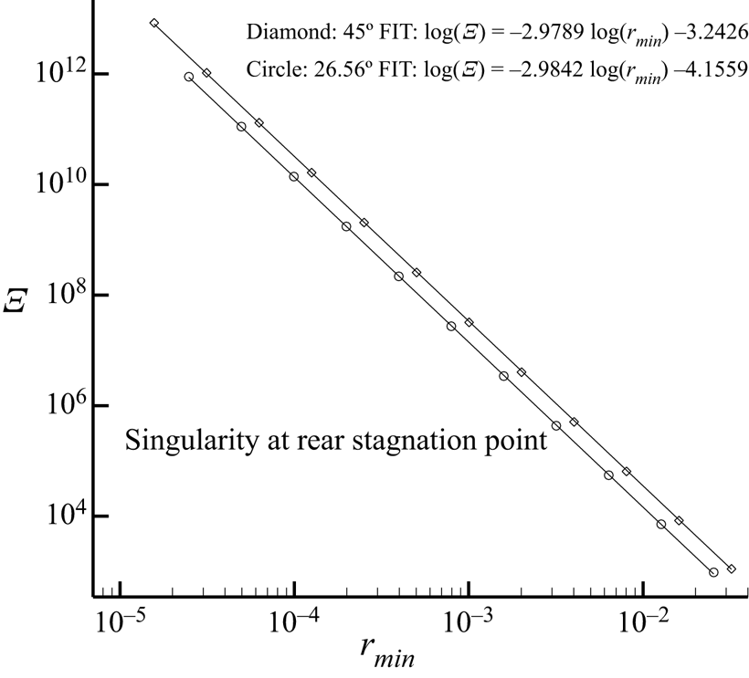
1. (1) In case 1, ${\boldsymbol{x}_0}$ is approaching the rear singularity (trailing edge or rear stagnation point). As ${\boldsymbol{x}_0}$ approaches the rear singularity (figure 2), the distance to the rear singularity behaves as $r \sim {r_{min}}$ asymptotically. Hence, $\varXi ({\boldsymbol{x}_0})$ diverges as ${r^{2 - 5/k}} \sim {r^{ - (2\tau /{\rm \pi} + 1)/(2 - \tau /{\rm \pi} )}}$ as ${\boldsymbol{x}_0}$ approaches the rear singularity. This singular behaviour had been already anticipated (including the dependence on the trailing edge angle) in Giles & Pierce (Reference Giles and Pierce1997), but no concrete predictions were made for the exponent. A 1/r_min singularity at the rear stagnation point was predicted in Lozano & Ponsin (Reference Lozano and Ponsin2021b) for blunt bodies in potential flow using the form of the streamline integral derived in Giles & Pierce (Reference Giles and Pierce1997), while the actual value for this case (for which $\tau = {\rm \pi} \Rightarrow k = 1$) is $\varXi \sim {r^{ - 3}}$.

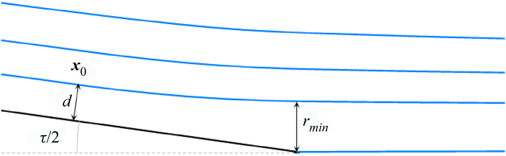
2. (2) In case 2, ${\boldsymbol{x}_0}$ is upstream of the rear singularity (figure 3). As ${\boldsymbol{x}_0}$ approaches the dividing streamline upstream of the rear singularity, $\varXi ({\boldsymbol{x}_0})$ diverges as $r_{\min }^{2 - 5/k} \sim {d^{k - 5/2}} \sim 1/{d^{\tau /{\rm \pi} + 1/2}}$, where d is the distance from ${\boldsymbol{x}_0}$ to the dividing streamline (incoming stagnation streamline or wall). Notice that the singularity exponent is not universal since it depends on the trailing edge angle $\tau $, and reduces to the inverse square-root behaviour predicted in Giles & Pierce (Reference Giles and Pierce1997) for cusped trailing edges (for which $\tau = 0$).

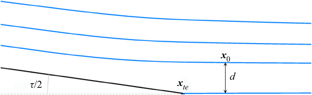
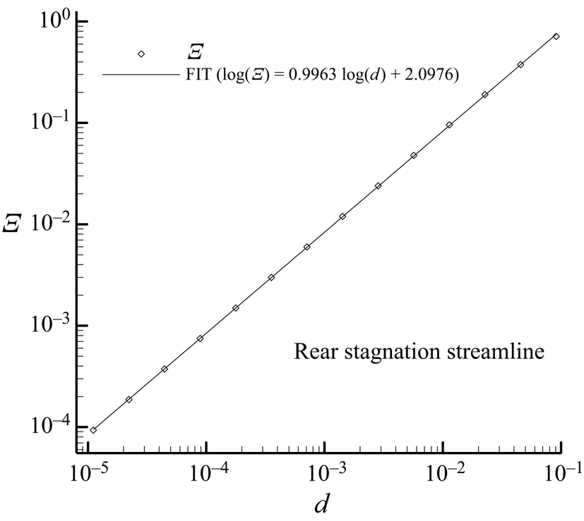
3. (3) In case 3, as ${\boldsymbol{x}_0}$ approaches the rear stagnation streamline downstream of the rear singularity (figure 4), $\varXi ({\boldsymbol{x}_0})$ does not diverge (the minimum distance from the streamline to the trailing edge is now $|{\boldsymbol{x}_0} - {\boldsymbol{x}_{te}}|$, which is always greater than zero) but rather behaves as $\varXi ({\boldsymbol{x}_0}) \sim d$, where d is the distance from ${\boldsymbol{x}_0}$ to the dividing streamline.

Figure 2.

Set-up for case 1.

Figure 3.

Set-up for case 2.

Figure 4.

Set-up for case 3.

The results of this asymptotic analysis are confirmed by actual computations (see § 5). This suggests that the origin of the divergence along the dividing streamline is the singularity at the trailing edge/rear stagnation point. This can be put on a firmer basis by noting that, as it will be shown later on, while the integral does get a small contribution from the leading-edge region, it is very approximately constant upstream of the rear singularity and vanishingly small downstream. Likewise, the integral behaves in exactly the same fashion at both the incoming stagnation streamline and the wall, with an exponent that depends on the local geometry around the rear singularity.

4.1.1. Influence of $\varXi $ on the sensitivity derivatives and the adjoint boundary conditions

The divergences of $\varXi $ (and ${\varUpsilon ^{(1)}}$ and ${\varUpsilon ^{(2)}}$) are propagated to the lift-based adjoint variables (4.6). However, two linear combinations of the adjoint variables,

(4.12)\begin{equation}\left. {\begin{array}{*{20}{c@{}}} {{I^{(1)}} = {\psi_1} + \boldsymbol{v}\boldsymbol{\cdot }({\psi_2},{\psi_3}) = ({q_\infty }{\varUpsilon^{(1)}} - u\sin \alpha + v\cos \alpha )/{c_\infty },}\\ {{I^{(2)}} = v{\psi_2} - u{\psi_3} = ( - v\sin \alpha - u\cos \alpha + {q_\infty }(1 + {\varUpsilon^{(2)}}))/{c_\infty },} \end{array}} \right\}\end{equation}

which yield the linearized perturbations to the lift due to a point source and a point vortex, respectively (Giles & Pierce Reference Giles and Pierce1997), remain finite except at the trailing edge. This fact is relevant since the adjoint variables enter the (continuous) adjoint-based sensitivity derivatives (2.12) precisely through ${I^{(1)}}$, which protects the sensitivities from diverging with mesh refinement (a fact that is well established numerically, see e.g. Lozano Reference Lozano2012, Reference Lozano2017, Reference Lozano2019b; Lozano & Ponsin Reference Lozano and Ponsin2022). Likewise, ${I^{(2)}}$ approaches $q\hat{n}_S \cdot ({\psi _2},{\psi _3})$ as the point approaches the wall and is thus directly related to the adjoint boundary condition, which is thus respected by the analytical solution and protected upon mesh refinement (Lozano Reference Lozano2019b). Finally, the divergence along the dividing streamline is encapsulated into a third (linearly independent) combination

(4.13)\begin{equation}{I^{(3)}} = ({\psi _1} + 2u{\psi _2} + 2v{\psi _3})/{q^2} = ({q_\infty }\varXi - 2{q^{ - 2}}u\sin \alpha + 2{q^{ - 2}}v\cos \alpha )/{c_\infty },\end{equation}

which yields the linearized perturbation to the lift due to a unit stagnation pressure point perturbation.

It is important to point out, however, that the above split of the adjoint solution space into protected and unprotected terms (as regards the dividing streamline singularity) is arbitrary and based on our choice of point perturbations (inherited from Giles & Pierce Reference Giles and Pierce1997). In fact, it turns out that any linear combination

(4.14)\begin{equation}a{\psi _1} + b{\psi _2} + c{\psi _3},\end{equation}

which corresponds to a point perturbation with source vector $f = {(a,b,c)^T}$, obeying $- a{q^2} + bu + cv = 0$, does not contain the streamline integral Ξ and is thus protected from the dividing streamline singularity. Conversely, if $- a{q^2} + bu + cv \ne 0$, then the corresponding perturbation is singular along the dividing streamline. One such example is $f = {(0,u,v)^T}$, which is related to the drag Eulerlet (Chadwick et al. Reference Chadwick, Christian, Kapoulas and Chalasani2019), a Green's function of the incompressible Euler equations linearized around a uniform flow which carries one unit of drag.

5.1. Circle

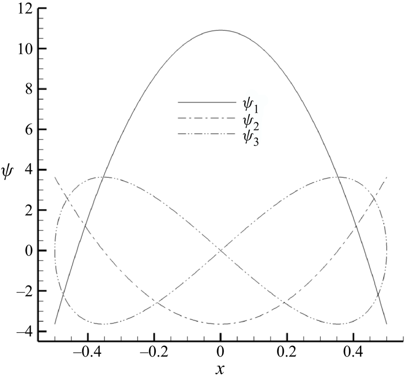
As explained above, obtaining meaningful adjoint solutions for bodies without sharp trailing edges, such as the circle, requires a Kutta condition to guarantee that the perturbations preserve the location of the rear stagnation point. As a consequence of this fact, the solutions (4.2) and (4.6) are applicable here, resulting in the analytic drag-based adjoint solution shown in figure 5.

Figure 5.

Analytic drag-based adjoint solution at the wall for incompressible, inviscid flow past a circle with ${\varGamma _0} = 0$.

Here and in what follows, the normalization of the adjoint variables is given by (4.2) and (4.6). For the flow variables, dimensions are fixed such that ${\rho _\infty } = 1 = {q_\infty }$, while spatial coordinates are normalized with the reference length $\ell$ (the diameter of the circle in this case).

To obtain the analytic lift-based adjoint solution, the streamline integral $\varXi ({\boldsymbol{x}_0})$ has to be evaluated at each point of the domain. As with Giles and Pierce's analytic quasi-1-D adjoint solution (Giles & Pierce Reference Giles and Pierce2001), this cannot be done in analytic form in general, so the solution has to be evaluated numerically instead. In the present case, there is the additional complication that the integration requires prior determination of the streamline passing through ${\boldsymbol{x}_0}$. Thus, to produce sample solutions, a numerical procedure must be assembled to trace the streamline and perform the integration. 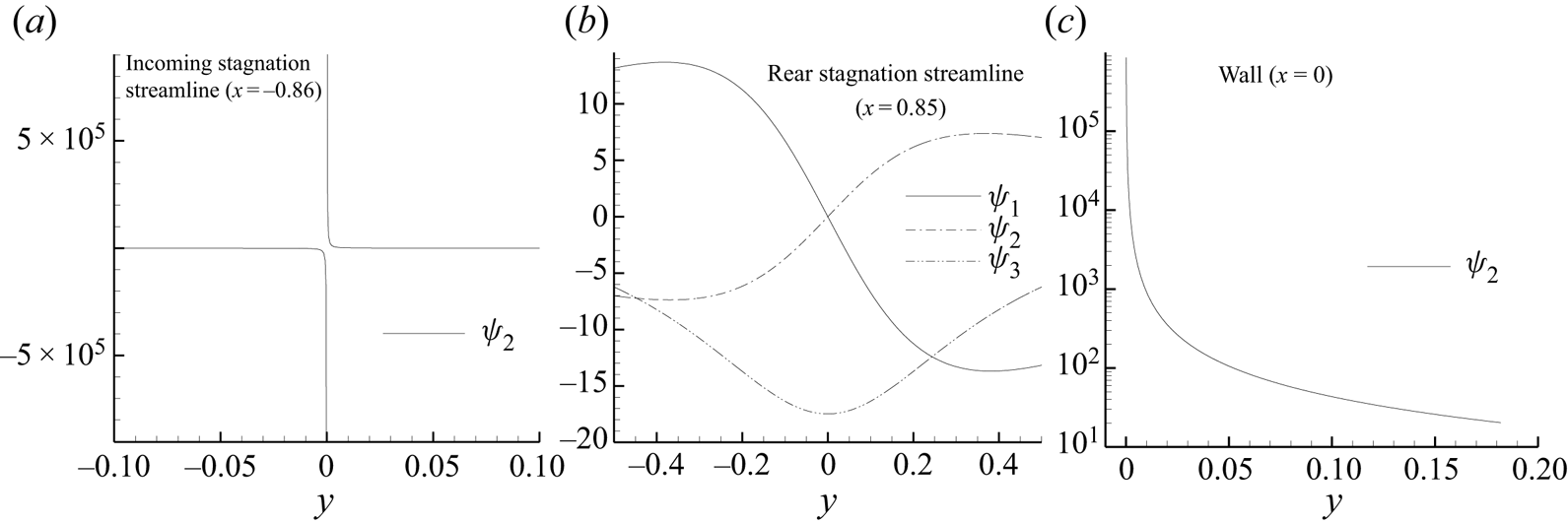Streamline tracing is carried out by direct numerical integration of the equation $\textrm{d}\boldsymbol{x}/\textrm{d}t = \boldsymbol{v}(\boldsymbol{x})$ with a fourth-order Runge–Kutta method (see e.g. Giles & Haimes Reference Giles and Haimes1990). The integration is carried out concurrently with a simple trapezoidal rule. Contour maps of the analytic lift-adjoint solution obtained in this way are shown in figure 6, while figure 7 shows the adjoint solution along three vertical lines crossing the stagnation streamline upstream and downstream of the circle and impinging the wall as indicated in figure 6. It is clear from both figures that the solution is singular along the dividing streamline upstream of the rear stagnation point (the circle wall and the incoming stagnation streamline), but not across the rear stagnation streamline.

Figure 6.

Analytic lift-based adjoint solution for incompressible, inviscid flow past a circle: (a) ${\psi _1}$; (b) ${\psi _2}$; (c) ${\psi _3}$.

Figure 7.

Analytic adjoint solution along vertical lines crossing the stagnation streamline upstream and downstream of the circle and impinging the wall as indicated in figure 6.

These singularities are caused by the streamline integral $\varXi $. In § 4, we argued that the streamline integral behaves as $\varXi \sim r_{min}^{2 - 5/k} \sim r_{min}^{ - (2\tau /{\rm \pi} + 1)/(2 - \tau /{\rm \pi} )}$ in terms of the distance of the streamline to the rear stagnation point/trailing edge. 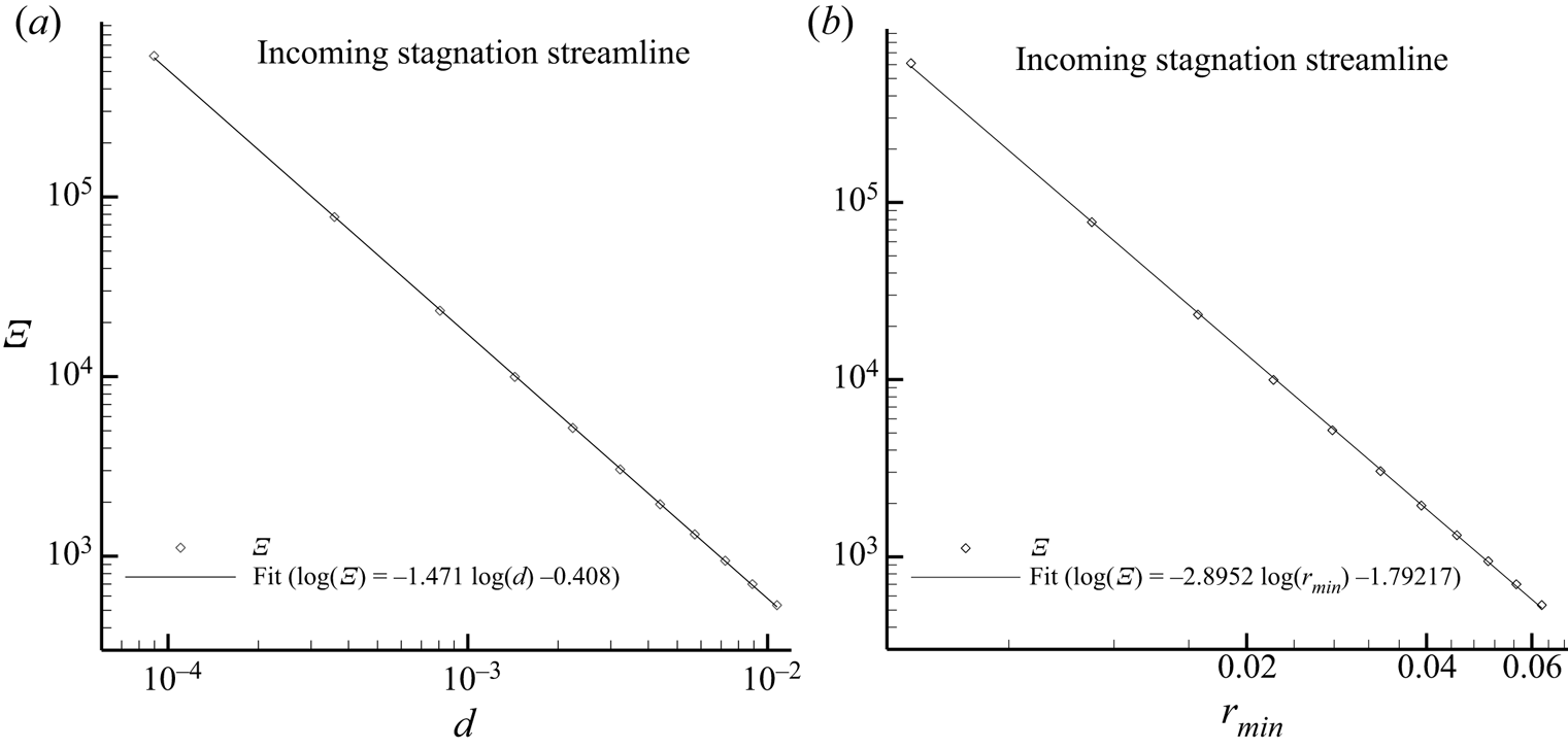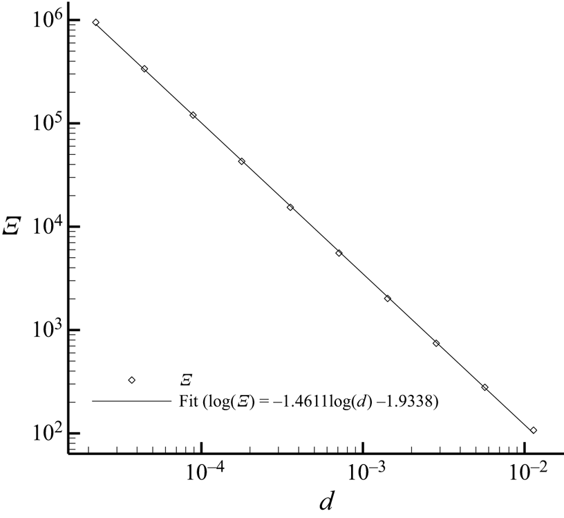Since k = 1 for the circle, we expect that $\varXi \sim r_{min}^{ - 3}$ at the rear stagnation point and $\varXi \sim {d^{ - 3/2}}$ at the wall and the incoming stagnation streamline, which is confirmed in figures 8–10. Figure 8 plots the value of the integral $\varXi $ at several points placed along a vertical line crossing the incoming stagnation streamline (the x axis) as indicated in figure 6. This value is fitted against the distance d to the stagnation streamline, yielding $\varXi \sim {d^{ - 1.47}}$, which is close to the theoretical prediction and to the value $\varXi \sim {d^{ - 1.46}}$ obtained at the wall (figure 9), but also against the minimum distance of the streamline to the rear stagnation point ${r_{min}}$, yielding $\varXi \sim r_{min}^{ - 2.9}$, which is close to the theoretical value and to the value of the exponent obtained for the rear stagnation point (figure 10). Finally, the integral vanishes linearly $\varXi \sim d$ across the rear stagnation streamline (figure 11), which is not singular.

Figure 8.

Value of the streamline integral computed with the analytic solution along a vertical line at x = −0.86 crossing the stagnation streamline upstream of the circle as indicated in figure 6. (a) Values of $\varXi$ versus distance d to the stagnation streamline. (b) Values of $\varXi$ versus minimum distance $r_{min}$ of the streamline to the rear stagnation point.

Figure 9.

Value of the streamline integral computed with the analytic solution along the vertical line x = 0 impinging the circle wall as indicated in figure 6.

Figure 10.

Value of the streamline integral computed with the analytic solution along two lines approaching the rear stagnation point with different inclinations as indicated in figure 6.

Figure 11.

Value of the streamline integral computed with the analytic solution along a vertical line at x = 0.85 crossing the stagnation streamline downstream of the circle as indicated in figure 6.

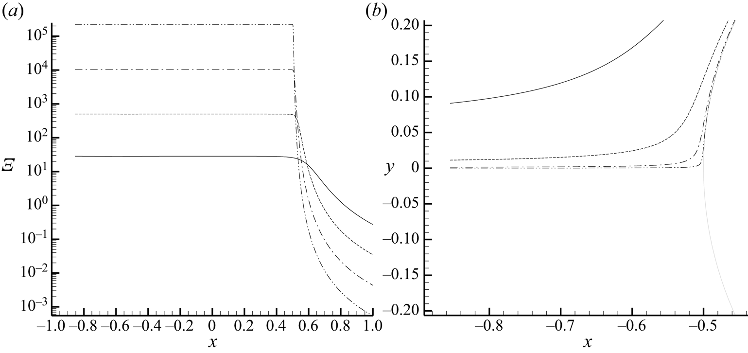
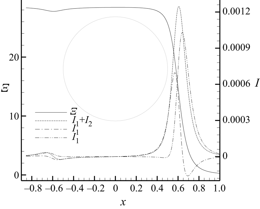
We have argued above that the behaviour at the wall and stagnation streamline is essentially governed by the singularity exponent at the rear singularity, which is thus the primary singularity. The results in figures 8 and 9 do support this idea, which is further illustrated with figures 12 and 13. Figure 12(a) shows the value of Ξ along the streamlines shown on the right plot. It can be clearly seen that the integral is quite approximately constant upstream of the trailing edge region and negligible downstream, and that the upstream value grows as the streamline approaches the dividing streamline (the downstream value, however, approaches zero), as expected. Figure 13, which focuses on the outermost streamline of figure 12, plots the running value of Ξ along the streamline, as well as $I ={-} {\partial _s}{q^{ - 2}}{\varUpsilon ^{(1)}} + 2{q^{ - 2}}{\partial _s}\phi (1 + {\varUpsilon ^{(2)}})$, which is the integrand in Ξ. It is clear that the main contribution to the integral comes from the region near the rear stagnation point, with a negligible contribution from the leading-edge region.

Figure 12.

(a) Running value of $\varXi ({\boldsymbol{x}_0})$ along the streamlines indicated in panel (b). The forward and rear stagnation points are located at $x ={-} 0.5$ and $x = 0.5$, respectively.

Figure 13.

Running value of $\varXi (\boldsymbol{x})$ and integrands ${I_1} ={-} {\partial _s}{q^{ - 2}}{\varUpsilon ^{(1)}},\;{I_2} = 2{\partial _s}\phi (1 + {\varUpsilon ^{(2)}})/{q^2}$ and $I = {I_1} + {I_2}$ along the outermost streamline of figure 12. The extension of the circle is indicated for reference purposes.

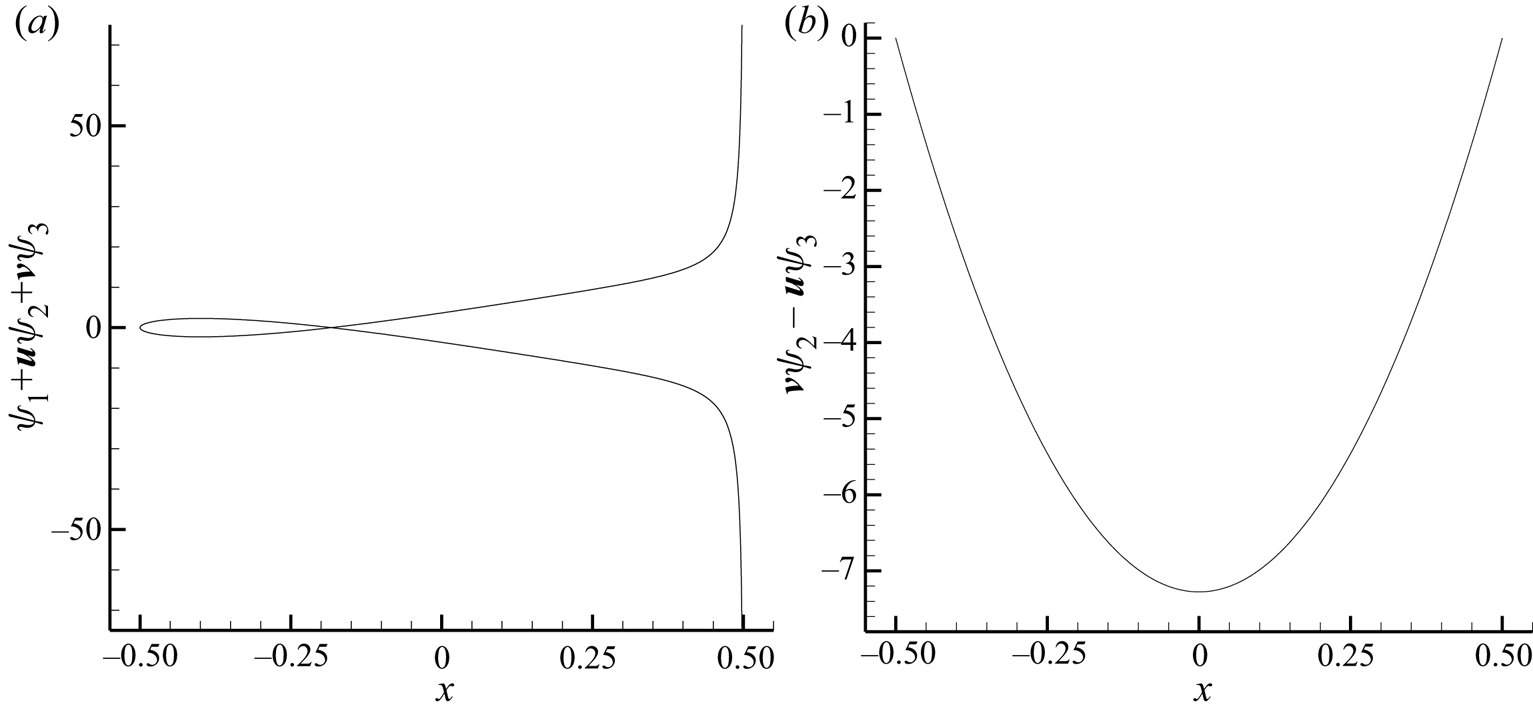
Finally, figure 14 plots the value of the linearized functionals ${I^{(1)}} = {\psi _1} + \boldsymbol{v}\boldsymbol{\cdot }({\psi _2},{\psi _3})$ and ${I^{(2)}} = v{\psi _2} - u{\psi _3}$ on the circle wall. These quantities have a finite value throughout the wall (except ${I^{(1)}}$, which diverges at the trailing edge), as expected.

Figure 14.

${I^{(1)}} = {\psi _1} + \boldsymbol{v}\boldsymbol{\cdot }({\psi _2},{\psi _3})$ and ${I^{(2)}} = v{\psi _2} - u{\psi _3}$ at the wall computed with the analytic lift-based adjoint solution for incompressible, inviscid flow past a circle.

5.2. Airfoil with finite trailing-edge angle

The second case involves incompressible, inviscid flow at an angle of attack α = 0° past a symmetrical van de Vooren airfoil given by the conformal transformation (Katz & Plotkin Reference Katz and Plotkin2001):

(5.1)\begin{equation}z = \frac{{{{(\zeta - R)}^k}}}{{{{(\zeta - \varepsilon R)}^{k - 1}}}} + 1,\end{equation}

where $R = {(1 + \varepsilon )^{k - 1}}/{2^k}$, $\varepsilon $ is a thickness parameter and k is related to the trailing-edge angle $\tau $ as $k = 2 - \tau /{\rm \pi} $. The transformation (5.1) maps the airfoil in the z plane to a circle of radius R centred at the origin in the $\zeta $ plane. 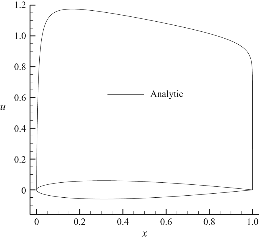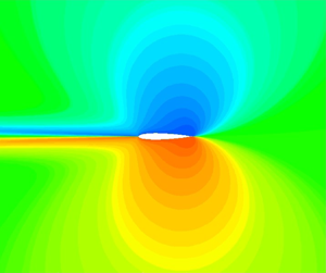In this paper, we set $\varepsilon = 0.0371$ and $k = 86/45$, resulting in an airfoil with 12 % thickness and finite trailing edge angle $\tau = 16^\circ$ that is shown in figure 15, where the analytic flow solution obtained with conformal transformation techniques is also depicted. The analytic flow solution can be found in Katz & Plotkin (Reference Katz and Plotkin2001) and can be obtained from the solution in the circle plane (3.10) and the transformation (5.1) as ${(u - iv)_{airfoil}} = (\textrm{d}\varPhi /\textrm{d}\zeta )/(\textrm{d}z/\textrm{d}\zeta )$.

Figure 15.

Geometry and analytic x-velocity for incompressible, inviscid flow at α = 0° past a van de Vooren airfoil with trailing-edge angle $\tau = 16^\circ$ and 12 % thickness computed with conformal transformation techniques. The flow is normalized such that ${\rho _\infty } = 1 = {q_\infty }$ and the airfoil profile is shown for reference.

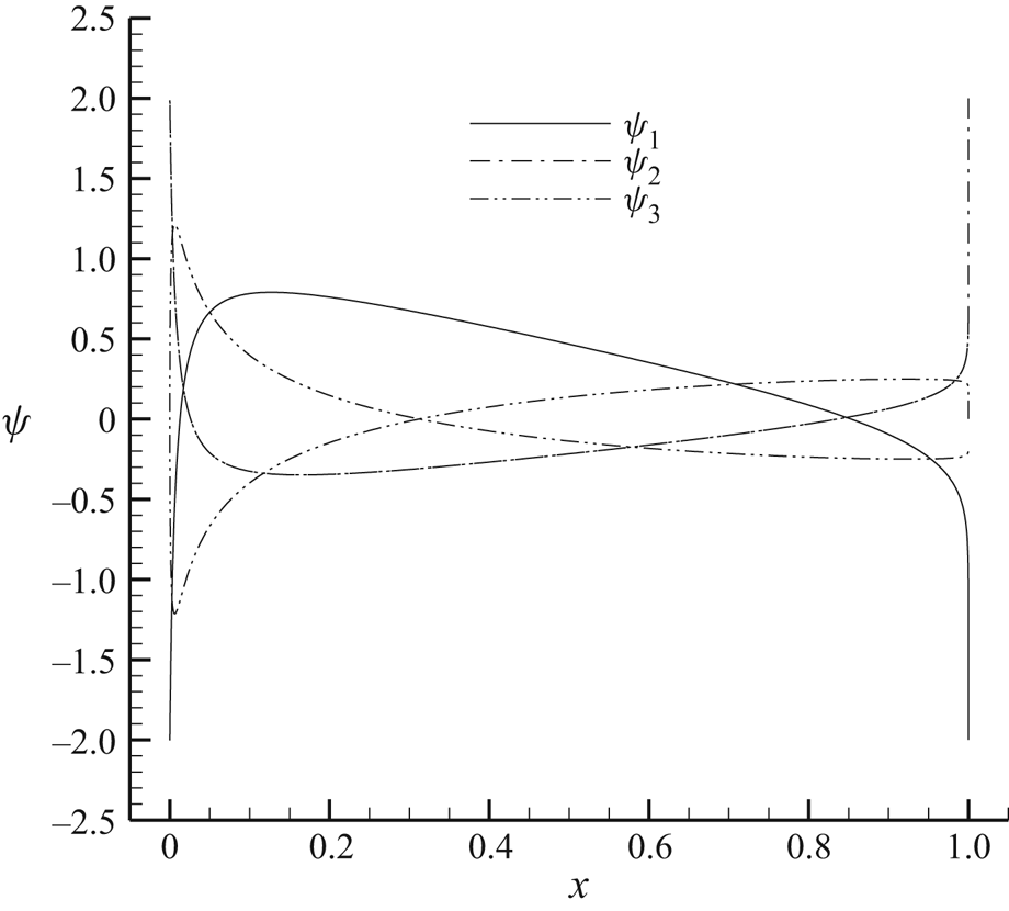
Using this analytic flow solution, the corresponding analytic adjoint solutions can be computed using (4.2) and (4.6). Figure 16 shows the analytic drag-based adjoint solution. This solution has been compared to numerical solutions obtained by discretizing the adjoint equation directly in Lozano & Ponsin (Reference Lozano and Ponsin2021a, Reference Lozano and Ponsin2022).

Figure 16.

Analytic drag-based adjoint solution on the airfoil profile for incompressible, inviscid flow at α = 0° past a van de Vooren airfoil with trailing-edge angle $\tau = 16^\circ$ and 12 % thickness.

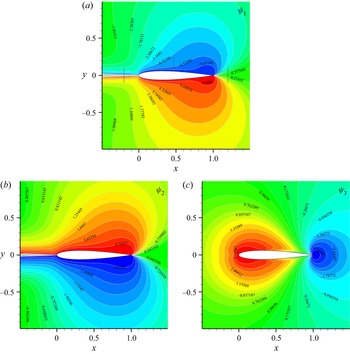
As for lift, the computation of the analytic adjoint solution is carried out with the fourth-order Runge–Kutta integrator described above. The streamline tracing is performed in the circle plane and then translated into the airfoil plane via the conformal transformation (5.1). Contour maps of the analytic lift adjoint solution obtained in this way are shown in figure 17. Again, a comparison of this solution to numerical adjoint solutions can be found in Lozano & Ponsin (Reference Lozano and Ponsin2022).

Figure 17.

Analytic lift-based adjoint solution for incompressible, inviscid flow at α = 0° past a van de Vooren airfoil with trailing-edge angle $\tau = 16^\circ$ and 12 % thickness: (a) ${\psi _1}$; (b) ${\psi _2}$; (c) ${\psi _3}$.

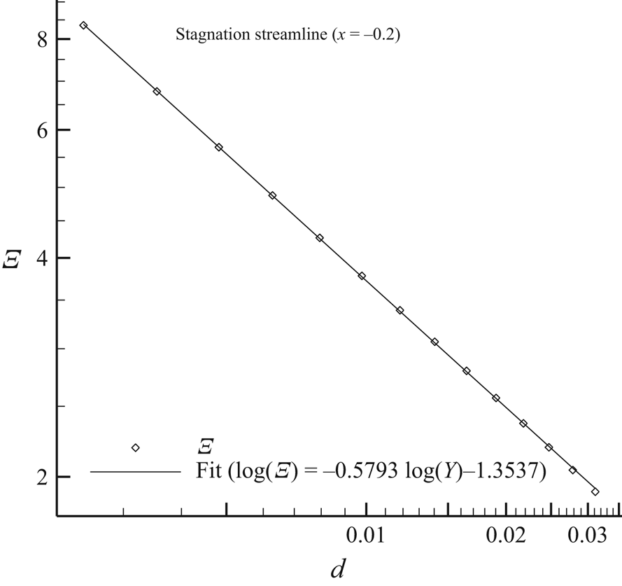
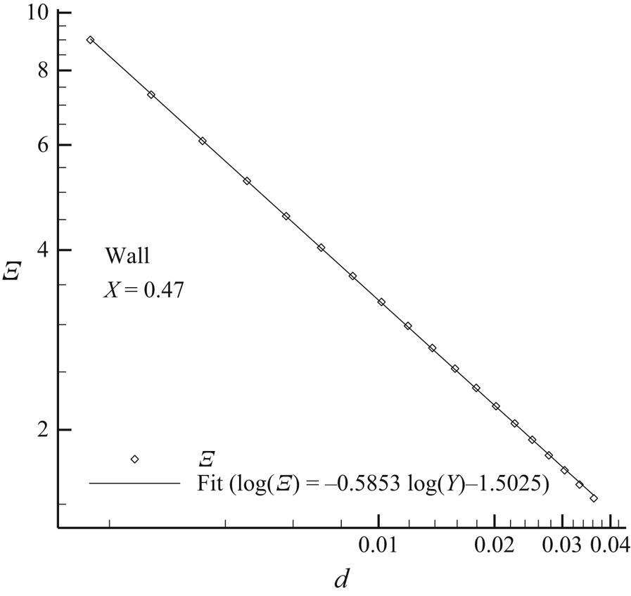
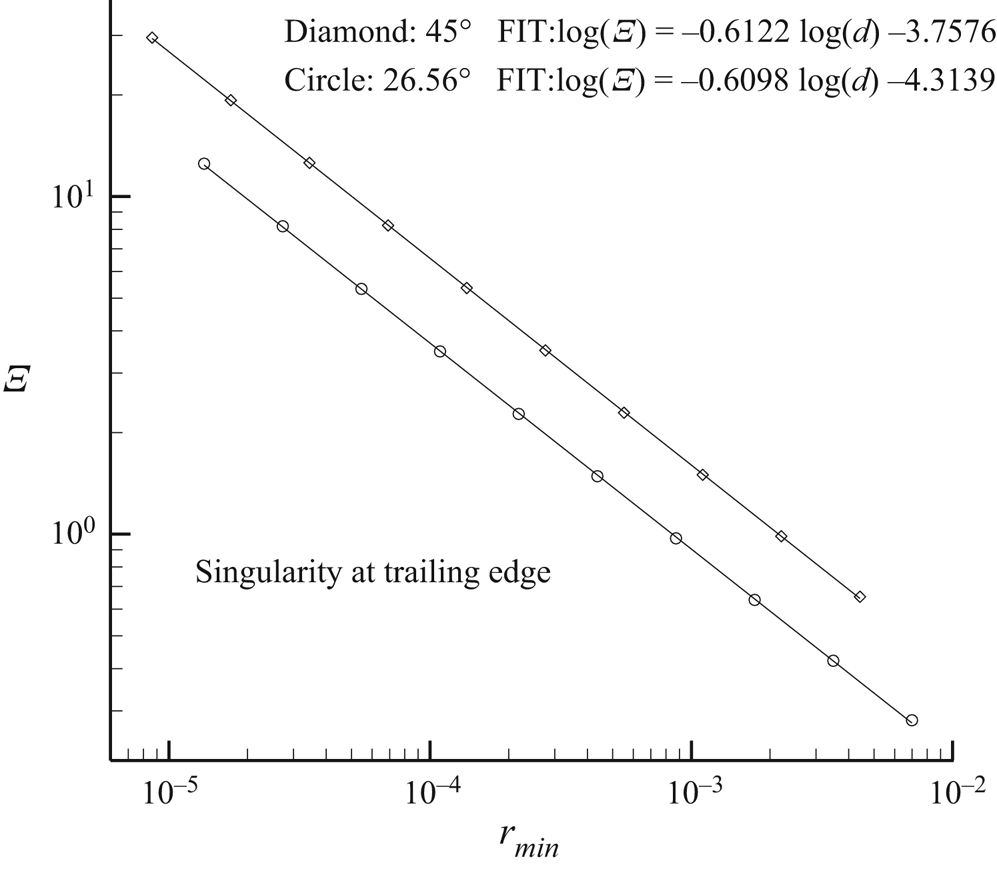
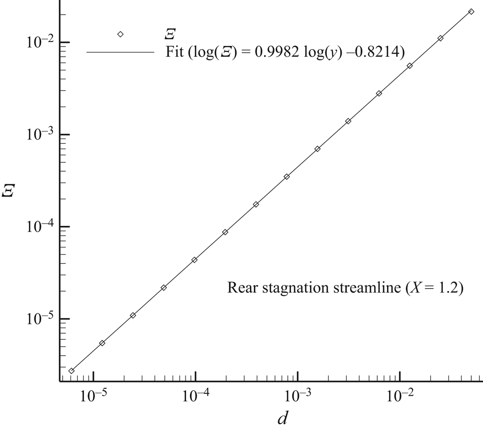
As in the circle case, the analytic solution shows singularities at the wall, across the incoming stagnation streamline and at the trailing edge, but not across the rear stagnation streamline. This is more clearly illustrated in figures 18–21, which plot the streamline integral $\varXi $ along lines approaching the stagnation streamline upstream of the airfoil, the wall, the trailing edge and the rear stagnation streamline, respectively, as indicated in figure 17. In all cases, the behaviour of the integral has been illustrated by fitting the curves to a power of the distance to the dividing streamline or the trailing edge as appropriate. At both the incoming stagnation streamline and the wall, the integral diverges as roughly $1/{d^{0.58}}$, where d is the distance to the stagnation streamline or to the wall. Noting that $k = 86/45$ for the present case, the exponent is close to the theoretical prediction $\varXi \sim 1/{d^{53/90}} = 1/{d^{0.589}}$. At the trailing edge, the integral shows a $1/{r^{0.61}}$ singularity (where r is the distance to the trailing edge) regardless of the inclination of the line, which is again in agreement with the theoretical prediction $\varXi \sim 1/{r^{53/86}} = 1/{r^{0.616}}$. Finally, the streamline integral vanishes as $\varXi \sim d$ at the stagnation streamline downstream of the trailing edge.

Figure 18.

Value of the streamline integral computed with the analytic solution along a line crossing the stagnation streamline upstream of the airfoil as indicated in figure 17.

Figure 19.

Value of the streamline integral computed with the analytic solution along a line impinging the airfoil as indicated in figure 17.

Figure 20.

Value of the streamline integral computed with the analytic solution along two lines approaching the trailing edge at different inclinations as indicated in figure 17.

Figure 21.

Value of the streamline integral computed with the analytic solution along a line crossing the stagnation streamline downstream of the airfoil as indicated in figure 17.

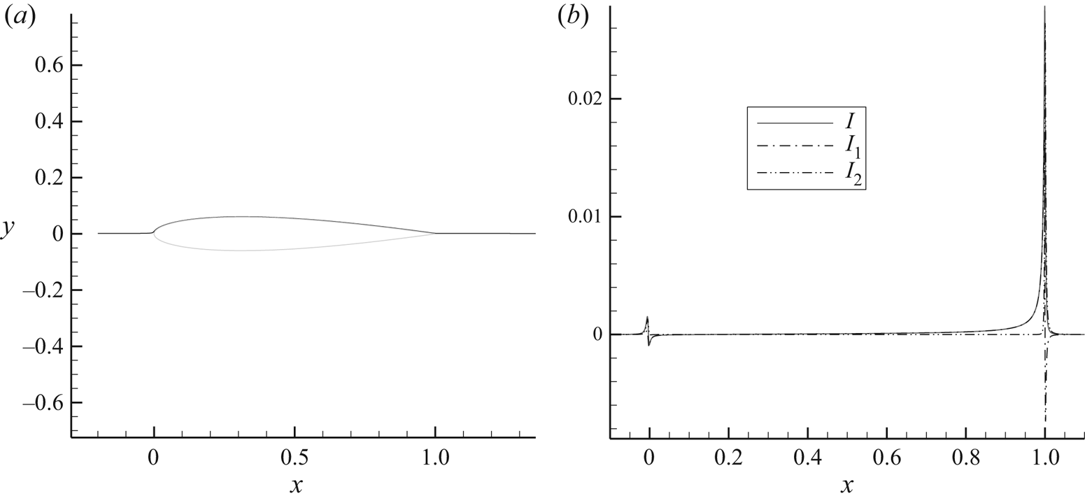
Figure 22 shows the value of $I ={-} {\partial _s}{q^{ - 2}}{\varUpsilon ^{(1)}} + 2{q^{ - 2}}{\partial _s}\phi (1 + {\varUpsilon ^{(2)}})$ along a streamline originating near the stagnation streamline upstream of the airfoil. It is clear, as in the previous case, that the main contribution to the integral comes from the region near the trailing edge, with a negligible contribution from the leading-edge region.

Figure 22.

Plot of ${I_1} ={-} {\partial _s}{q^{ - 2}}{\varUpsilon ^{(1)}},\;{I_2} = 2{\partial _s}\phi (1 + {\varUpsilon ^{(2)}})/{q^2}\;\textrm{and}\;I = {I_1} + {I_2}$ for the streamline shown in panel (a). Inviscid, incompressible flow at α = 0° past a van de Vooren airfoil with trailing-edge angle $\tau = 16^\circ$ and 12 % thickness.

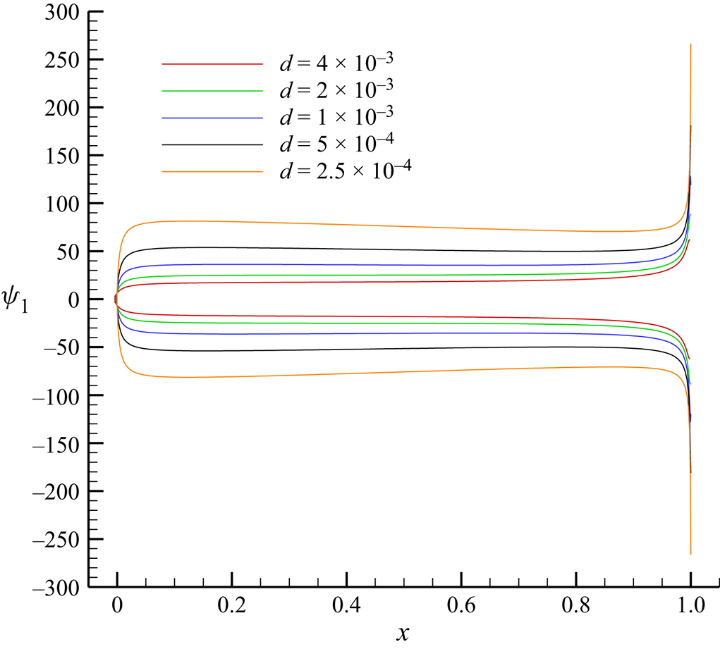
To end the analysis of the airfoil solution, figure 23 focuses on the behaviour of the adjoint solution near the airfoil profile. In the plot, the first component of the analytic adjoint solution is shown for a succession of O-shaped curves surrounding the van der Vooren airfoil profile and progressively closer to it, clearly demonstrating the divergence of the analytic solution at the wall. It is clear that the anomaly observed in numerical computations (Lozano Reference Lozano2019b; Lozano & Ponsin Reference Lozano and Ponsin2022; Peter et al. Reference Peter, Renac and Labbé2022) is caused by a divergence of the analytic solution at the wall. On the numerical side, the numerical viscosity of the solver stabilizes the divergence, producing a finite value at the profile which nevertheless varies continually as the grid spacing or the intensity of the numerical dissipation change (Lozano & Ponsin Reference Lozano and Ponsin2021b). 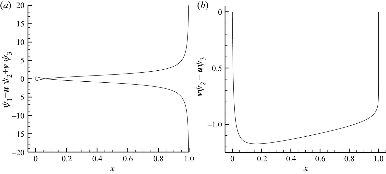At any rate, while the adjoint variables diverge at the wall, the linearized functionals ${I^{(1)}}$ and ${I^{(2)}}$ (4.12) are again finite across the profile (except ${I^{(1)}}$ which diverges at the trailing edge) as shown in figure 24.

Figure 23.

Analytic lift-based adjoint solution for incompressible, inviscid flow at α = 0° past a van de Vooren airfoil with trailing-edge angle $\tau = 16^\circ$ and 12 % thickness on a sequence of O-shaped curves progressively approaching the airfoil.

Figure 24.

(a) ${I^{(1)}} = {\psi _1} + \boldsymbol{v}\boldsymbol{\cdot }({\psi _2},{\psi _3})$ and (b) ${I^{(2)}} = v{\psi _2} - u{\psi _3}$ on the airfoil profile computed with the analytic lift-based adjoint solution for incompressible, inviscid flow at α = 0° past a van de Vooren airfoil with trailing-edge angle $\tau = 16^\circ$ and 12 % thickness.